HAL Id: hal-01132440https://hal.archives-ouvertes.fr/hal-01132440

Submitted on 21 Apr 2015

HAL is a multi-disciplinary open accessarchive for the deposit and dissemination of sci-entific research documents, whether they are pub-lished or not. The documents may come fromteaching and research institutions in France orabroad, or from public or private research centers.

L’archive ouverte pluridisciplinaire HAL, estdestinée au dépôt et à la diffusion de documentsscientifiques de niveau recherche, publiés ou non,émanant des établissements d’enseignement et derecherche français ou étrangers, des laboratoirespublics ou privés.

Homological Reconstruction and Simplification in R3Dominique Attali, Ulrich Bauer, Olivier Devillers, Marc Glisse, André Lieutier

To cite this version:Dominique Attali, Ulrich Bauer, Olivier Devillers, Marc Glisse, André Lieutier. Homological Recon-struction and Simplification in R3. Computational Geometry, Elsevier, 2015, 48 (8), pp.606-621.�10.1016/j.comgeo.2014.08.010�. �hal-01132440�

Homological Reconstruction and Simplification in R3

Dominique Attali

Gipsa-lab, Saint Martin d’Hères, France

Ulrich Bauer⇤

IST Austria, Klosterneuburg, Austria

Olivier Devillers

INRIA Sophia Antipolis – Méditerranée, Sophia Antipolis, France

Marc Glisse

INRIA Saclay – Île-de-France, Orsay, France

André LieutierDassault Système, Aix-en-Provence, France

Abstract

We consider the problem of deciding whether the persistent homology group of asimplicial pair (K, L) can be realized as the homology H⇤(X) of some complex X withL ⇢ X ⇢ K. We show that this problem is NP-complete even if K is embedded in R3.

As a consequence, we show that it is NP-hard to simplify level and sublevel sets ofscalar functions on S3 within a given tolerance constraint. This problem has relevanceto the visualization of medical images by isosurfaces. We also show an implication tothe theory of well groups of scalar functions: not every well group can be realized bysome level set, and deciding whether a well group can be realized is NP-hard.

Keywords: NP-hard problems, homology, persistence2010 MSC: 55U10

⇤Corresponding author.Email addresses: mail@ulrich-bauer.org (Ulrich Bauer ), Andre.LIEUTIER@3ds.com (André

Lieutier)URL: http://www.gipsa-lab.grenoble-inp.fr/ (Dominique Attali),

http://ulrich-bauer.org (Ulrich Bauer ),http://www-sop.inria.fr/members/Olivier.Devillers/ (Olivier Devillers),http://geometrica.saclay.inria.fr/team/Marc.Glisse/ (Marc Glisse)

Preprint submitted to Elsevier October 10, 2014

1. Introduction

In this paper, we establish NP-completeness of a variety of related problems that askfor an object in R3 with certain prescribed topological constraints.

In the most basic setting, we have a point cloud in Rd that samples a shape andwant to retrieve information on the sampled shape. There exists a whole spectrumof possibilities regarding the type of sought information. At the coarsest level, wecan content ourselves with the homology groups which record the “holes” of a givendimension, hereafter referred to as homological features (connected components, cycles,cavities and so on). At a finer level, we may be interested in building an approximationof the shape, reflecting as accurately as possible both its geometry and topology. Thestandard way is to construct a simplicial complex using the data points as vertices, suchas for instance the ↵-complex, the Rips complex or the Cech complex [13, 12]. All threeconstructions have in common to depend upon a scale parameter ↵ and to get biggeras ↵ increases. In the ideal case, we expect the complex to have the right homologyfor some suitable value of ↵ [21, 6, 7, 2]. Unfortunately, depending on the sampling, itmay happen that such a value of ↵ does not exist. Nonetheless, we might still be able toinfer the true homology of the shape hidden in the noisy data using persistent homology[15, 10, 8]. Given two scale parameters ↵1 and ↵2, the persistent homology groupsrecord the homological features that persist from ↵1 to ↵2. Under very weak hypotheses,we know that the persistent homology is precisely that of the sampled shape [10, 5].The persistent homology can be computed e�ciently (i.e., in polynomial time).

A natural question is then to ask for a complex that carries the persistent homology:given a complex K and a subcomplex L, can we find a subcomplex of K that contains Land whose homological features are precisely those common to L and K? Our answer isthat sometimes we cannot, and deciding whether we can is NP-complete. This answerwas first given in the general case by Attali and Lieutier [1], who posed the restrictionto complexes embedded in R3 as an open problem. We resolve this problem by provingNP-completeness even for complexes embedded in R3.

The above problem concentrates on building a complex whose homology matchesperfectly the persistent homology of L into K: all the homological noise has beenremoved. We call such an object a homological reconstruction. However, when it doesnot exist, it is still relevant to look for a complex nested between L and K and whosehomology is as close as possible to the persistent homology of L into K: as much noiseas possible has been removed. We call such a complex a homological simplification andprove that finding one is also an NP-hard problem.

In the field of visualization and image analysis, another common setting consists indescribing a shape through a continuous function f : Rd ! R instead of a point cloudin Rd. For instance, a medical image may be a collection of density measurements overa grid of 3D points and is best modeled as a continuous map over a certain domain of R3.In the ideal case, the shape is a sublevel set of the function, f �1(�1, t]. Unfortunately,noise can plague the data. As the parameter t increases, sublevel sets inflate and wecan track the evolution of their homology. Features that appear and disappear quicklyare considered topological noise, and we can consider the common features of twosublevel sets as those of a denoised sublevel set. The question now becomes: can we findanother cleaner function, close enough to the original one, whose sublevel set has the

2

Figure 1: Example of a simplicial pair (K, L) embedded in R3 that has no homological reconstruction.

denoised homology, i.e., a sublevel set reconstruction? The corresponding optimizationproblem asks for a sublevel set simplification, i.e., a function close to the original onethat minimizes the number of homological features of the sublevel set. We show thatthese two problems are the equivalents in the functional setting to the homologicalreconstruction and simplification of simplicial pairs described above.

Often, one is also interested in the homology of a level set, f �1(t). We showhow it can be related to the (persistent) homology of sublevel sets, and consider thecorresponding level set reconstruction/simplification problems.

Further in this direction, Edelsbrunner et al. introduced the well group [16, 3] as adenoised version of the homology group of a level set. Again, we can ask whether onecan find a realization of the well group, i.e., a cleaner function whose level set has thesame homology as the well group?

We shall see in this paper that all of these related problems are NP-hard, as aconsequence of the NP-completeness of the homological reconstruction problem.

1.1. Background and notationsWe are only concerned with topological spaces that are triangulable by a finite

simplicial complex, so simplicial and singular homology are isomorphic and we make nodistinction between the two. In particular, we use the simplicial versions of the Excisionand Mayer-Vietoris sequence theorems, which have less restrictive assumptions thantheir singular counterparts. If K is an abstract simplicial complex, we denote by K itsgeometric realization. Throughout this article, we consider homology with coe�cientsin an arbitrary field F, so the homology groups are finite-dimensional F-vector spacesand there is no torsion. Note that for simplicial complexes K embedded in R3, this isin fact not a restriction, since due to the absence of torsion in R3 the Betti numbers areindependent of the choice of coe�cients (see, e.g., [17, §3.3]).

Given a topological space K , we write H⇤(K) =L

i Hi(K) for the direct sum ofhomology groups in all dimensions, and �(K) =

Pi�0 �i(K) for the total Betti number.

If (K ,L) is a pair of topological spaces L ⇢ K , the inclusion L ,! K induces ahomomorphism H⇤(L) ! H⇤(K), which is denoted by H⇤(L ,! K). The rank ofthis map is the persistent Betti number of the inclusion L ,! K and is denoted by�(L ,! K) = rank H⇤(L ,! K); the image im H⇤(L ,! K) is a persistent homologygroup. If (K, L) is a simplicial pair, that is, a pair of simplicial complexes such thatL ⇢ K, then the persistent Betti number �(L ,! K) can be computed in time cubic in

3

Figure 2: Example of a simplicial pair (left) having a homological reconstruction as a subspace (right), butnot as a subcomplex. The simplicial complex on the left contains three tetrahedra sharing an edge and whoseunion forms a triangular bipyramid.

the number of simplices in K [15]. This cubic complexity can be improved to matrixmultiplication time [19].

A piecewise linear function on a topological space K is a continuous functionf : K ! R such that there exists a finite triangulation of K on which f is simplexwiselinear. Note that a simplexwise linear function must be linear on each simplex of thegiven triangulation, while a piecewise linear function is linear on each simplex of somearbitrary triangulation.

2. Reconstruction and simplification of simplicial pairs

In this section, we consider a simplicial pair and define the homological reconstruc-tion problem and the homological simplification problem. We prove that both problemsare NP-hard when the simplicial pair is embedded in R3. We start with a simple lemma:

Lemma 1. Consider a triple of topological spacesL ⇢ X ⇢ K with finite Betti numbers.Then

�(X) � �(L ,! K).

Proof. This is a consequence of the fact that whenever we consider two linear mapsj : U ! V and i : V ! W between finite dimensional vector spaces, then dim V �rank j � rank i � j. ⇤

This property suggests the following definition:

Definition 1. Consider a triple of topological spaces L ⇢ X ⇢ K with finite Bettinumbers. ThenX is called a homological reconstruction of (K ,L) if �(X) = �(L ,! K).Moreover, X is called a homological p-reconstruction of (K ,L) if �p(X) = �p(L ,! K).

We will often omit “homological” since there is no ambiguity in this paper. Anequivalent condition for X being a reconstruction is that H⇤(L ,! X) is surjective andH⇤(X ,! K) is injective, as defined in [1]. Not every pair (K ,L) admits a reconstruction;a simple counterexample is shown in Fig. 1. The use of topological spaces in thedefinition (as opposed to simplicial complexes) is motivated by the following observation.Let (K, L) be a simplicial pair. Then there might be a reconstruction of (K, L), but notas a subcomplex of K. An example is shown in Fig. 2. A reconstruction that is a

4

subcomplex is called a subcomplex reconstruction. To emphasize the distinction tothis case, we sometimes use the term subspace reconstruction to emphasize that thereconstruction is only required to be a subspace, not necessarily a subcomplex.

2.1. Homological reconstruction is NP-hardWe now focus our attention on spaces that are geometric realizations of finite

simplicial complexes embedded in R3.

Theorem 1. The homological reconstruction problem is NP-hard: Given as input asimplicial pair (K, L) embedded in R3, decide whether there exists a subspace recon-struction X of (K, L). The problem is NP-complete if X is required to be a subcomplex.

This section is devoted to the proof of Theorem 1 by reduction from 3-SAT. Recallthat a Boolean formula � is in 3-CNF if it is a conjunction of several clauses, each ofwhich is a disjunction of three literals, a literal being either a variable or its negation.Given a 3-CNF formula �, we construct a simplicial pair (K�, L�) embedded in R3 andprove that (K�, L�) has a reconstruction (as a subcomplex of K�) if and only if � has asatisfying assignment (see Lemmas 2 and 3 below).

For this, we associate to the 3-CNF formula � a simplicial pair (K�, L�) withtrivial persistent homology. Equivalently, any reconstruction X of (K�, L�) has trivialhomology, i.e.,

�d(X) = �d(L� ,! K�) =

8>><>>:

1 if d = 0,0 otherwise.

This means that X has a single connected component, no loops, and no cavities. X hasto fill all loops or cavities in L� and has to connect the di↵erent connected componentsof L� by adding to L� portions of K� without creating any new loops or cavities.

The variable gadget. The variable gadget is a simplicial pair (Vi,Wi) as depicted inFig. 3, top. The simplicial complex Vi contains 4 edges forming a cycle. The two boldedges do not belong to Wi. One of the bold edges will be called Truei and the other onewill be called Falsei. The key property of this construction is that any reconstruction ofthe pair (Vi,Wi) cannot contain both edges Truei and Falsei, for otherwise they wouldform a 1-cycle with the remaining edges. This property will allow us to match thepresence of the edge Truei to a true assignment of the variable vi.

The clause gadget. The clause gadget is a simplicial pair (C j,Dj) as depicted in Fig. 3,bottom. The simplicial complex Dj contains a cycle ABCDE. The cycle is closed withtwo surfaces in C j (thereafter referred to as the lower hemisphere and the disk) therebycreating a cavity. Furthermore, the complex Dj contains an arc that ends inside the disk.Whenever we fill the cycle ABCDE with the disk, this connects the two endpoints of thearc, thus creating a new cycle, which we close twice in C j by a left hemisphere and aright hemisphere. Consider one bold edge in the interior of each hemisphere, which iswhere the clause gadget will connect to the variable gadgets.

The key property of this clause gadget is that at least one of the 3 bold edges mustbe present in any reconstruction X of the pair (C j,Dj). Indeed, the cycle ABCDE in Xmust be filled up. If it is filled by the lower hemisphere, we are done. If it is filled by

5

Truei Falsei

Vi Wi

A

BC

DE

FG

H

A

BC

DE

FG

H

C j Dj

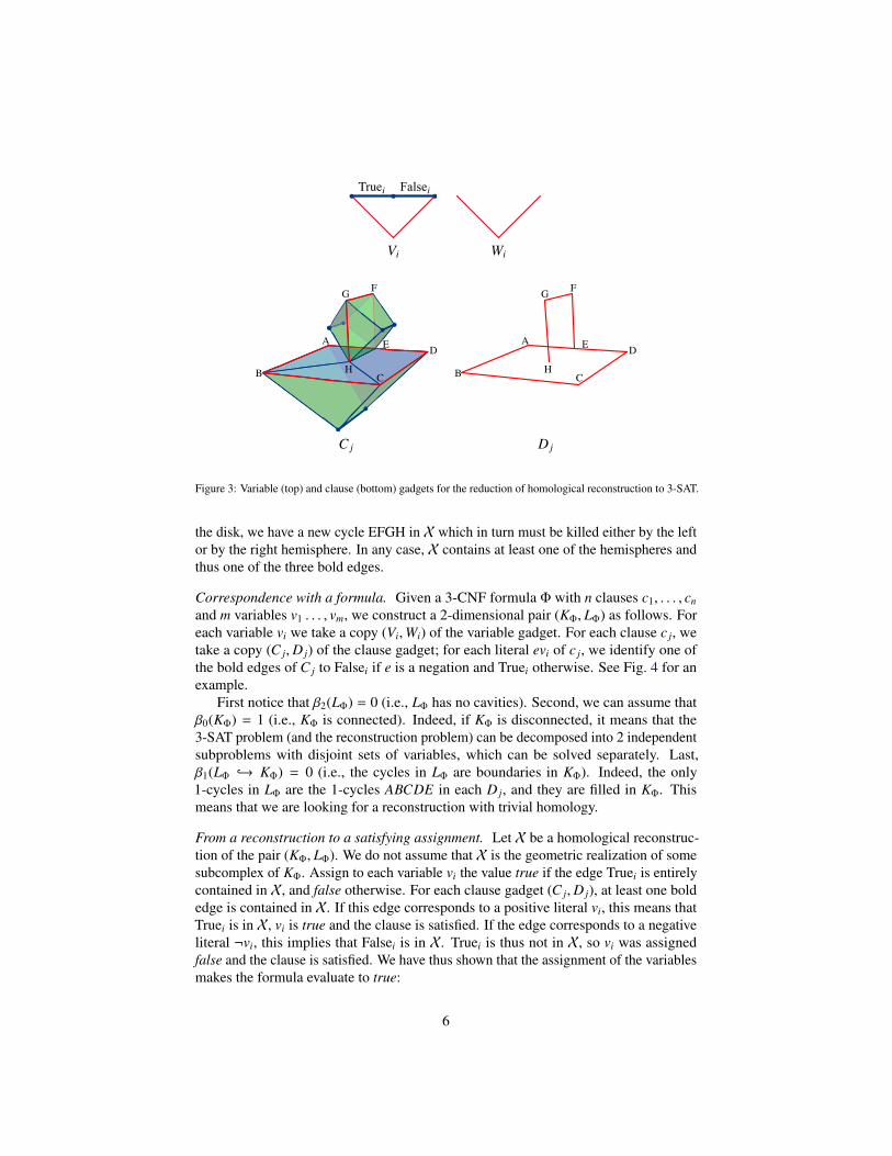
Figure 3: Variable (top) and clause (bottom) gadgets for the reduction of homological reconstruction to 3-SAT.

the disk, we have a new cycle EFGH in X which in turn must be killed either by the leftor by the right hemisphere. In any case, X contains at least one of the hemispheres andthus one of the three bold edges.

Correspondence with a formula. Given a 3-CNF formula � with n clauses c1, . . . , cnand m variables v1 . . . , vm, we construct a 2-dimensional pair (K�, L�) as follows. Foreach variable vi we take a copy (Vi,Wi) of the variable gadget. For each clause c j, wetake a copy (C j,Dj) of the clause gadget; for each literal evi of c j, we identify one ofthe bold edges of C j to Falsei if e is a negation and Truei otherwise. See Fig. 4 for anexample.

First notice that �2(L�) = 0 (i.e., L� has no cavities). Second, we can assume that�0(K�) = 1 (i.e., K� is connected). Indeed, if K� is disconnected, it means that the3-SAT problem (and the reconstruction problem) can be decomposed into 2 independentsubproblems with disjoint sets of variables, which can be solved separately. Last,�1(L� ,! K�) = 0 (i.e., the cycles in L� are boundaries in K�). Indeed, the only1-cycles in L� are the 1-cycles ABCDE in each Dj, and they are filled in K�. Thismeans that we are looking for a reconstruction with trivial homology.

From a reconstruction to a satisfying assignment. Let X be a homological reconstruc-tion of the pair (K�, L�). We do not assume that X is the geometric realization of somesubcomplex of K�. Assign to each variable vi the value true if the edge Truei is entirelycontained in X, and false otherwise. For each clause gadget (C j,Dj), at least one boldedge is contained in X. If this edge corresponds to a positive literal vi, this means thatTruei is in X, vi is true and the clause is satisfied. If the edge corresponds to a negativeliteral ¬vi, this implies that Falsei is in X. Truei is thus not in X, so vi was assignedfalse and the clause is satisfied. We have thus shown that the assignment of the variablesmakes the formula evaluate to true:

6

(¬t _ u_ v)

(t _¬v_¬w)

(¬u_¬v_w)

t

uv

w

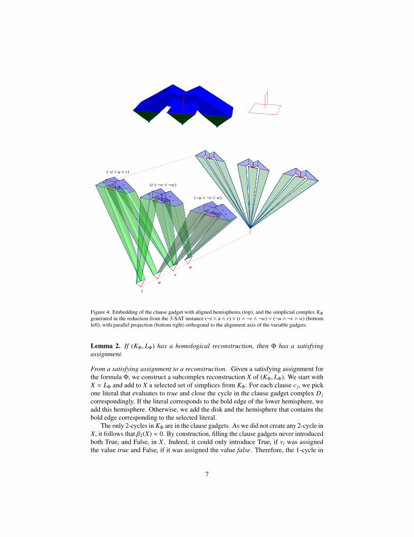
Figure 4: Embedding of the clause gadget with aligned hemispheres (top), and the simplicial complex K�generated in the reduction from the 3-SAT instance (¬t ^ u ^ v) _ (t ^ ¬v ^ ¬w) _ (¬u ^ ¬v ^ w) (bottomleft), with parallel projection (bottom right) orthogonal to the alignment axis of the variable gadgets.

Lemma 2. If (K�, L�) has a homological reconstruction, then � has a satisfyingassignment.

From a satisfying assignment to a reconstruction. Given a satisfying assignment forthe formula �, we construct a subcomplex reconstruction X of (K�, L�). We start withX = L� and add to X a selected set of simplices from K�. For each clause c j, we pickone literal that evaluates to true and close the cycle in the clause gadget complex Djcorrespondingly. If the literal corresponds to the bold edge of the lower hemisphere, weadd this hemisphere. Otherwise, we add the disk and the hemisphere that contains thebold edge corresponding to the selected literal.

The only 2-cycles in K� are in the clause gadgets. As we did not create any 2-cycle inX, it follows that �2(X) = 0. By construction, filling the clause gadgets never introducedboth Truei and Falsei in X. Indeed, it could only introduce Truei if vi was assignedthe value true and Falsei if it was assigned the value false. Therefore, the 1-cycle in

7

the variable gadgets do not appear in X. Also, for each clause gadget, we filled theABCDE 1-cycle, and whenever we created an extra EFGH 1-cycle by adding the disk,we immediately filled it with the left or right hemisphere. Now we only need to checkthat the construction did not create any “non-local” 1-cycles. Since for each clausewe have only used one of the literals which evaluate to true, the only contact a clausegadget in X has with the rest of X is through a single bold edge, and the clause gadgetcan be collapsed to that edge. After collapsing all clause gadgets, all that remains aredisconnected variable gadgets with at most 3 edges each, and so �1(X) = 0. We finallyadd to X just enough edges from K� so that it becomes connected, without creating anyextra cycles in the process. This is possible since we assumed that K� is connected.Thus we have �0(X) = 1. We conclude:

Lemma 3. If � has a satisfying assignment, then (K�, L�) has a subcomplex recon-struction.

We are now in a position to prove Theorem 1.

Proof of Theorem 1. First we show that the homological reconstruction problem is NP-hard. We proceed by reduction from 3-SAT. Let (K, L) = (K�, L�) be a simplicial pairdefined by a 3-SAT instance �. We show that the following propositions are equivalent:

(a) (K, L) has a subspace reconstruction;

(b) � has a satisfying assignment;

(c) (K, L) has a subcomplex reconstruction.

The implication (a) =) (b) is shown in Lemma 2; (b) =) (c) is shown in Lemma 3.Finally, (c) =) (a) is trivial.

The pair (K, L) can be constructed from � in time polynomial in the size of �. To-gether with the equivalence (a)() (b), this establishes NP-hardness of the homologicalreconstruction problem.

The equivalence (b)() (c) also yields NP-hardness of the subcomplex reconstruc-tion problem. Moreover, given a subcomplex X as a polynomial size certificate, we candecide in polynomial time whether X is a reconstruction of (K, L). Thus the problem isalso in NP and hence NP-complete. ⇤

Embedding. Later, we have to consider not only an embedding of K�, but also atriangulation of its complement. The following fact will be useful:

Lemma 4. There is a triangulation of S3 with size polynomial in the size of K� andhaving K� as a subcomplex.

Proof. First, referring to Fig. 4, it is clear that K� can be embedded in R3. Indeed, wecan align the clause gadgets and the variable gadgets along two lines parallel to thecoordinate axes and make each clause gadget look like a small body with three longtentacles that connect to the variable gadgets. Due to the way the variable and clausegadgets are aligned in the construction along skew axes, the tentacles do not intersect intheir interior.

8

Variable gadget

TrueFalse

Clause gadget

¬tt

¬uu

¬vv

¬ww

(¬t _ u_ v) (t _¬v_¬w) (¬u_¬v_w)

Figure 5: Example of 3-SAT reduction using a 3D grid embedding.

We can subdivide the space by first projecting K� onto a plane orthogonal to the linecarrying the variable gadgets. We get a polygonal region whose complement can easilybe triangulated inside a bounding box without adding any new vertex and thus adding alinear number of edges. Extending each triangle in the direction of the projection, weget a collection of tubes, one for each triangle. The tubes can easily be triangulatedwhile respecting K� to obtain a polynomial size triangulation of a bounding box ofthe construction, which can trivially be extended to a polynomial size triangulationof S3. ⇤

We want to remark that a similar construction can be realized even if we restrictedges and faces of L and K to be edges and faces of a 3D grid (see Fig. 5). This meansthat a variant of Theorem 1 can also be shown for cubical complexes arising from 3Dimage data.

Corollary 1. The homological simplification problem is NP-hard: Given as input asimplicial pair (K, L) embedded in R3, find a complex X minimizing �(X) subject toL ⇢ X ⇢ K.

Proof. We use a reduction from the subcomplex reconstruction problem. To determineif a subcomplex reconstruction exists, we can first find a complex X minimizing �(X)subject to L ⇢ X ⇢ K. We then only need to check if its Betti number matches the lowerbound �(L ,! K). ⇤

3. Reconstruction and simplification of level and sublevel sets

In this section, we consider a real-valued simplexwise linear function defined on asimplicial complex embedded in R3 and establish the NP-hardness of problems that askfor a nearby function with a simplified sublevel set (Section 3.1) and a simplified levelset (Section 3.3).

Given a real-valued function f , we write Ft for the t-level set f �1(t), Ft for the(closed) t-sublevel set f �1((�1, t]), and F<t for the open t-sublevel set f �1((�1, t)). In

9

–2

0 0

0 –2

–2

–2

–2

–2

–2

–2

0

–2

–1 –1

–1 –2

–2

–2

–2

–2

–2

–2

1

Figure 6: Top: A simplicial pair (K, L) and a homological reconstruction of (K, L) as a subcomplex. Bottom:values of f (left) and g (right) at the vertices of the barycentric subdivision sd K, as used in the proof ofTheorem 2.

this paper we shall only consider real-valued piecewise linear functions. Note that leveland sublevel sets of a simplexwise linear function on a simplicial complex K are notnecessarily subcomplexes of K, but subcomplexes of an appropriate subdivision of K.Moreover, we have the following property:

Proposition 1 (Kühnel [18], Morozov [20]). Let f be a simplexwise linear functionon a simplicial complex K. Let K(t) be the induced subcomplex of K on {v 2 vert K :f (v) t}. Then K(t) is homotopy equivalent to the sublevel set Ft. If t , f (v) for allv 2 vert K, then K(t) is also homotopy equivalent to the open sublevel set F<t.

Definition 2. Let f , g be piecewise linear functions and consider real parameters t and�. The function g is called a sublevel set (t, �)-reconstruction of f if kg � f k1 � andGt is a reconstruction of the pair (Ft+�, Ft��), i.e.,

�(Gt) = �(Ft�� ,! Ft+�).

Note thatFt�� ✓ Gt ✓ Ft+�,

so that�(Gt) � �(Ft�� ,! Ft+�).

A sublevel set (t, �)-reconstruction is thus also a minimizer of �(Gt) subject to kg �f k1 �.

3.1. Sublevel set reconstruction is NP-hardTheorem 2. The sublevel set reconstruction problem is NP-hard: Given as input asimplexwise linear function f on a simplicial complex embedded in R3 and parameterst and �, decide whether there exists a sublevel set (t, �)-reconstruction g of f .

10

Proof. It su�ces to establish the theorem for t = 0 and � = 1. We proceed by reductionfrom 3-SAT using the results of the previous section. Let (K, L) = (K�, L�) be a simpli-cial pair defined by a 3-SAT instance �, as described in the proof of Theorem 1. Weconstruct an instance of the level set simplification problem by defining a simplexwiselinear function f : sd K ! R on the barycentric subdivision of K; see Figure 6. Recallthat the barycentric subdivision (or derived subdivision) of a simplicial complex K isthe order complex of the face relation, i.e., the abstract simplicial complex sd K whosevertices are the simplices of K and whose simplices are the totally ordered subsets of Kwith regard to the face relation. We define f via its values on the vertices of sd K. Usingthe fact that a vertex � of sd K is a simplex of K, we let

f : � 7!8>><>>:�2 if � 2 L,0 otherwise.

(1)

Note that for every function g with kg � f k1 1, the 0-sublevel set G0 containsL and is contained in K. We show that the following propositions are equivalent topropositions (a)–(c) in the proof of Theorem 1:

(d) f has a simplexwise linear sublevel set (0, 1)-reconstruction g.

(e) f has a sublevel set (0, 1)-reconstruction g.

To show (c) =) (d), we define a simplexwise linear function g on sd K by its values onthe vertices of sd K (the simplices of K); see Figure 6:

g : � 7!

8>>>>><>>>>>:

�2 if � 2 L,�1 if � 2 X \ L,1 if � 2 K \ X.

(2)

We have kg � f k1 = 1. By Proposition 1, the sublevel set G0 is homotopy equivalentto |X| and hence is a reconstruction of the pair

(K, L) ' (F1, F�1).

Finally, (d) =) (e) is trivial and (e) =) (a) follows directly with G0 as a reconstructionof (F1, F�1) ' (K, L).

The function f can be constructed from the 3-SAT instance � in polynomial time.Together with the equivalence (b)() (e), this establishes NP-hardness of the sublevelset reconstruction problem.

The equivalence (b)() (d) also yields NP-hardness of the sublevel set reconstruc-tion problem restricted to simplexwise linear functions sd K ! R. ⇤

Theorem 3. The sublevel set reconstruction problem is NP-complete if the reconstruc-tion is required to be simplexwise linear on the same complex.

Proof. By Theorem 2, it is su�cient to show that the problem is in NP, i.e. every“yes” instance f : K ! R has certificate with size polynomial in the size of K and f .Again, it su�ces to establish the theorem for t = 0 and � = 1. We show that there is

11

a simplexwise linear (0, 1)-reconstruction g i↵ there is a subset of vertices S whoseinduced subcomplex KS is a reconstruction of (K(1),K(�1)), where K(t) is the inducedsubcomplex of K on {v 2 vert K : f (v) t} as in Proposition 1.

The subset of vertices v with g(v) 0 induces a subcomplex that is homotopyequivalent to the sublevel set G0, by Proposition 1. Vice versa, let S be a subset ofvertices such that the induced subcomplex KS is a reconstruction of (K(1),K(�1)). Inparticular, for all v 2 S we have f (v) 1, and for all v < S we have f (v) > �1. Define asimplexwise linear function by the vertex values

h : v 7!8>><>>:

f (v) � 1 if v 2 S ,f (v) + 1 if v < S ,

and note that for each vertex v, h(v) 0 if and only if v 2 S . By Proposition 1, thesublevel set H0 is homotopy equivalent to the induced subcomplex KS and henceis a reconstruction of the pair (F1, F�1) ' (K(1),K(�1)). We conclude that h is a(0, 1)-reconstruction of f .

Given a subset S as a polynomial size certificate, by computing and comparing �(KS )and �(K(�1) ,! K(1)) we can verify in polynomial time the existence of a sublevel set(0, 1)-reconstruction of f . Thus the problem is also in NP and hence NP-complete. ⇤

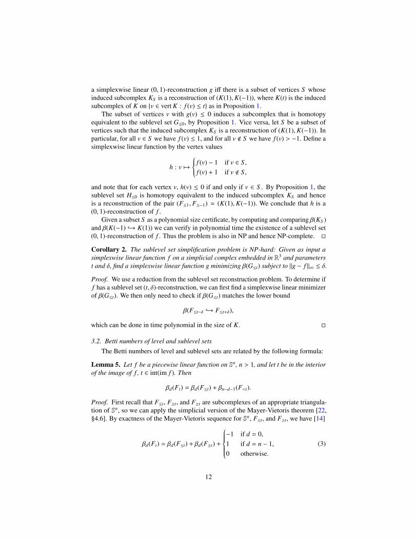
Corollary 2. The sublevel set simplification problem is NP-hard: Given as input asimplexwise linear function f on a simplicial complex embedded in R3 and parameterst and �, find a simplexwise linear function g minimizing �(Gt) subject to kg � f k1 �.

Proof. We use a reduction from the sublevel set reconstruction problem. To determine iff has a sublevel set (t, �)-reconstruction, we can first find a simplexwise linear minimizerof �(Gt). We then only need to check if �(Gt) matches the lower bound

�(Ft�� ,! Ft+�),

which can be done in time polynomial in the size of K. ⇤

3.2. Betti numbers of level and sublevel setsThe Betti numbers of level and sublevel sets are related by the following formula:

Lemma 5. Let f be a piecewise linear function on Sn, n > 1, and let t be in the interiorof the image of f , t 2 int(im f ). Then

�d(Ft) = �d(Ft) + �n�d�1(F<t).

Proof. First recall that Ft, F�t, and F�t are subcomplexes of an appropriate triangula-tion of Sn, so we can apply the simplicial version of the Mayer-Vietoris theorem [22,§4.6]. By exactness of the Mayer-Vietoris sequence for Sn, Ft, and F�t, we have [14]

�d(Ft) = �d(Ft) + �d(F�t) +

8>>>>><>>>>>:

�1 if d = 0,1 if d = n � 1,0 otherwise.

(3)

12

By Alexander duality [17, §3.3], the duality of homology and cohomology with fieldcoe�cients resulting from the universal coe�cient theorem [17, §3.1], and isomorphismof dual finite-dimensional vector spaces, we have

eHd(F�t) � eHn�d�1(F<t) � Hom(eHn�d�1(F<t),F) � eHn�d�1(F<t),

where eHd denotes the dth reduced homology group and Hom(eHn�d�1(F<t),F) is the dualvector space of eHn�d�1(F<t), i.e., the linear maps to F. Recall that

�d(X) = rank(eHd(X)) +

8>><>>:

1 if d = 0,0 otherwise.

We thus have

�d(F�t) = �n�d�1(F<t) +

8>>>>><>>>>>:

1 if d = 0,�1 if d = n � 1,0 otherwise.

(4)

By combining Eqs. (3) and (4), we obtain the stated equality. ⇤

For all piecewise linear functions f , g on Sn with kg � f k1 � and t ± � 2 int(im f ),we have t 2 int(im g) and thus by Lemmas 1 and 5,

�(Gt) � �(Ft�� ,! Ft+�) + �(F<t�� ,! F<t+�).

This motivates the following definition:

Definition 3. Let f , g be piecewise linear functions on Sn and consider real parameterst and � with t ± � 2 int(im f ). The function g is called a level set (t, �)-reconstructionof f if kg � f k1 � and

�(Gt) = �(Ft�� ,! Ft+�) + �(F<t�� ,! F<t+�).

A level set (t, �)-reconstruction is thus also a minimizer of �(Gt) subject to kg� f k1 �. Since the above equality can only be achieved if both inequalities

�(Gt) � �(Ft�� ,! Ft+�) and�(G<t) � �(F<t�� ,! F<t+�)

derived from Lemma 1 hold with equality, we conclude:

Lemma 6. Let f , g be piecewise linear functions on Sn. If g is a level set (t, �)-reconstruction of f , then

�(Gt) = �(Ft�� ,! Ft+�)�(G<t) = �(F<t�� ,! F<t+�)

and in particular g is also a sublevel set (t, �)-reconstruction of f .

We will show in the following that sublevel set reconstructions are also level setreconstructions, under some additional hypotheses.

13

3.3. Level set reconstruction is NP-hardDefinition 4. Let f be a piecewise linear function. A homological regular value of f isa number t 2 R such that H⇤(F<t ,! Ft) is an isomorphism.

We remark that there exist several other notions of regularity in the literature, whichdo not match our definition when extended to general functions [10, 4]. For piecewiselinear functions however, all these definitions are equivalent. Note also that regularityshould be understood with respect to sublevel sets; t can be a regular value t even thoughH⇤(F>t ,! F�t) might not be an isomorphism.

Lemma 7. Let f be a piecewise linear function on Sn, n > 1. If t ± � 2 int(im f ) areregular values of f and g is a level set (t, �)-reconstruction of f , then t is a regular valueof g.

Proof. By hypothesis t ± � are regular values of f , so

H⇤(F<t�� ,! Ft��) and H⇤(F<t+� ,! Ft+�)

are isomorphisms and

�(F<t�� ,! F<t+�) = �(F<t�� ,! Ft+�) = �(Ft�� ,! Ft+�).

Since g is a level set (t, �)-reconstruction of f , by Lemma 6, we have

�(Gt) = �(Ft�� ,! Ft+�) and�(G<t) = �(F<t�� ,! F<t+�)

and hence�(Gt) = �(G<t) = �(F<t�� ,! Ft+�).

Observing thatF<t�� ⇢ G<t ⇢ Gt ⇢ Gt+�

and using the fact that whenever we have three linear maps

U ! V ! W ! X

between finite-dimensional vector spaces, then

rank(U ! X) rank(V ! W),

we get�(F<t�� ,! Ft+�) �(G<t ,! Gt) �(Gt).

Combining all these relations, we deduce that

�(Gt) = �(G<t) = �(G<t ,! Gt) = �(Gt).

and conclude that H⇤(G<t ,! Gt) is an isomorphism. ⇤

14

Lemma 8. Let f and g be piecewise linear functions on Sn, n > 1. Assume thatt ± � 2 int(im f ) are regular values of f and t 2 int(im g) is a regular value of g.Then g is a sublevel set (t, �)-reconstruction of f if and only if g is a level set (t, �)-reconstruction of f .

Proof. By hypothesis, t is a regular value of g. Substituting into Lemma 5, we obtainthe first equation below; the second equation comes from the fact that t ± � are regularvalues of f :

2�(Gt) = �(Gt),2�(Ft�� ,! Ft+�) = �(Ft�� ,! Ft+�) + �(F<t�� ,! F<t+�).

By definition, g is a sublevel set (t, �)-reconstruction of f if and only if the left handsides of the two equations above are equal. Similarly, g is a level set (t, �)-reconstructionif and only if the right hand sides of the two equations above are equal. The resultfollows immediately. ⇤

Theorem 4. The level set reconstruction problem is NP-hard: Given as input a simplex-wise linear function on a triangulation of S3 and parameters t and �, decide whetherthere exists a level set (t, �)-reconstruction g of f . The problem is NP-complete if g isrequired to be simplexwise linear on this triangulation.

Proof. We reuse the same reduction as in Theorem 2. Since we need functions definedon the sphere, we triangulate the complement of K to obtain a triangulation S of thesphere with size polynomial in the size of K and K ⇢ S as in Lemma 4. We extend ffrom Eq. (1) to a simplexwise linear function f on sd S :

f : � 7!8>><>>:

f (�) if � 2 K,2 otherwise.

We then prove that propositions (a)–(e) in the proofs of Theorems 1 and 2 and (f), (g)below are equivalent.

(f) f has a simplexwise linear level set (0, 1)-reconstruction g.

(g) f has a level set (0, 1)-reconstruction g.

We trivially have (f) =) (g). Now we prove that (g) =) (d). Proposition 1 implies thatthe values ±1 are regular values of f . By Lemma 7, the value 0 is a regular value ofg. Lemma 8 then proves that g is a sublevel set reconstruction of f . Now let g be therestriction of g to K. Since the sublevel sets Ft and eFt are homotopy equivalent fort 1, and the sublevel sets Gt and eGt are homotopy equivalent for t 0, it followsthat g is a sublevel set reconstruction of f .

Next, we prove that (c) =) (f). Given a subcomplex reconstruction X of (K, L), wedefine g using Eq. (2) and extend it to g : sd S ! R as above for f . Since 0 is a regularvalue of g, Lemma 8 implies that g is a level set reconstruction.

In analogy to the proof of Theorem 2, we obtain NP-hardness of the level setreconstruction problem and NP-completeness of the problem restricted to simplexwiselinear functions. ⇤

15

Corollary 3. The level set simplification problem is NP-hard: Given a piecewise linearfunction f on S3 and parameters t and �, find a simplexwise linear function g minimizing�(Gt) subject to kg � f k1 �.Proof. To determine if f has a level set (t, �)-reconstruction, we can first find a minimizerof �(Gt). We then only need to check if �(Gt) matches the lower bound

�(Gt) = �(Gt) + �(G<t) �(Ft�� ,! Ft+�) + �(F<t�� ,! F<t+�),

which can be done in time polynomial in the size of the underlying triangulation. ⇤

4. Realizations of well groups

We now discuss how the previous results relate to the concept of well groups, whichwere introduced in [16] as a robust version of the homology group of a level set.

Let f : K ! R be a piecewise linear function. For � � 0 and an interval [a, b] ⇢ R ,the ([a, b], �)-well group of f is defined as

W⇤( f , [a, b], �) =\

g:kg� f k1�im H⇤(G[a,b] ,! F[a��,b+�]),

where F[a,b] = f �1([a, b]). In fact, as shown in [3], the well group is already given bythe intersection of just two persistent homology groups:

W⇤( f , [a, b], �) = im H⇤(F[a��,b��] ,! F[a��,b+�])\ im H⇤(F[a+�,b+�] ,! F[a��,b+�]).

(5)

The following formula expresses the rank of the well group in terms of persistent Bettinumbers using relative homology.

Theorem 5 (Bendich et al. [3]). Let f : K ! R be a piecewise linear function and leta b and � 2 R be such that a ± �, b ± � are regular values of f . Then

rank W⇤( f , [a, b], �) = �(Fb�� ,! Fb+�)� �((Fb��, ;) ,! (K , F�a+�))+ �((K , F�a+�) ,! (K , F�a��))� �((Fb+�, ;) ,! (K , F�a��)).

We are particularly interested in the case where the interval consists of a single point.We call W⇤( f , t, �) = W⇤( f , [t, t], �) the (t, �)-well group of f . Intuitively, it captures thehomology common to all perturbed level sets.

Clearly, the rank of the well group provides a lower bound on the Betti number ofthe t-level set of any g with kg � f k1 �:

�(Gt) � �(Gt ,! F[t��,t+�]) � rank W⇤( f , t, �).

We say that the well group is realized by such a function g if

�(Gt) = rank W⇤( f , t, �),

or equivalently, if H⇤(Gt ,! F[t��,t+�]) maps H⇤(Gt) bijectively to W⇤( f , t, �). As we willshow in Theorem 6, this lower bound cannot always be achieved, and hence not everywell group is realizable.

16

4.1. Realizability of well groups is NP-hardWe now show that on Sn, a realization of a well group is the same as a level set

reconstruction:

Theorem 6. Let f be a piecewise linear function on Sn with t ± � 2 int(im f ). Apiecewise linear function g realizes the well group W⇤( f , t, �) if and only if it is a levelset (t, �)-reconstruction of f .

Proof. The number of critical values of f is finite, and so for every s 2 R, there is ✏ > 0such that all values in [s � ✏, s) and in (s, s + ✏] are regular, and hence

H⇤(Fs�✏ ,! F<s) and H⇤(Fs ,! Fs+✏)

are isomorphisms. Choose ✏ such that the above holds for s = t ± �. Let a = t � ✏ andb = t + ✏. Now a ± �, b ± � are regular values and we can apply Theorem 5.

The second and forth terms in the formula of Theorem 5 vanish. To see this, notethat t ± � 2 int(im f ) implies

Fb±� = Ft+✏±� ( Sn

for ✏ small enough, and thus �n(Fb±�) = 0. Similarly,

F�a±� = F�t�✏±� , ;and thus �0(Sn, F�a±�) = 0. Moreover, �d(Sn) = 0 for d < {0, n}. Since the inducedhomomorphisms

H⇤((Fb±�, ;) ,! (Sn, F�a⌥�))factor as

H⇤(Fb±�)! H⇤(Sn)! H⇤(Sn, F�a⌥�),we have

�((Fb±�, ;) ,! (Sn, F�a⌥�)) = 0.Moreover, by the duality theorem of extended persistence on manifolds [11], we can

rewrite the third term in Theorem 5 as

�d((Sn, F�a+�) ,! (Sn, F�a��)) = �n�d(Fa�� ,! Fa+�).

Finally, by regularity of the values [a±�, t±�) and (t±�, b±�], we have isomorphisms

H⇤(Ft±� ,! F[a±�,b±�]) and H⇤(F[t��,t+�] ,! F[a��,b+�])

and thus by Eq. (5)W⇤( f , t, �) � W⇤( f , [a, b], �).

Altogether, this yields

rank W⇤( f , t, �) = �(Ft�� ,! Ft+�) + �(F<t�� ,! F<t+�).

The statement now follows directly from the definitions. ⇤

Together with Theorem 4, we have:

Corollary 4. The well group realization problem is NP-hard: Given a piecewise linearfunction f : K ✓ S3 ! R and parameters t and �, decide whether the well groupW⇤( f , t, �) can be realized. The problem is NP-complete if the realization is required tobe simplexwise linear on K.

17

5. An easy case

In this section, we discuss an important special case in which the subcomplexreconstruction problem can in fact be solved in polynomial time.

5.1. Building a p-reconstruction of an easily p-reconstructible pairWe start by presenting a polynomial time algorithm which outputs a p-reconstruction

of the pair (K, L), assuming that (K, L) is p-reconstructible and enjoys an easinessproperty that we describe below.

Definition 5. Given a simplicial complex K and a subcomplex L, we say that (K, L) isan easily p-reconstructible pair if

(a) (K, L) is p-reconstructible and

(b) for all subcomplexes X such that L ✓ X ✓ K, the homomorphism Hp�1(X ,! K)induced by the inclusion X ✓ K is injective.

Condition (b) is equivalent to requiring that for every filtration F containing thetwo simplicial complexes L and K, no (p � 1)-cycle is destroyed in F between L andK. In other words, each time a p-simplex is added in F between L and K, it creates ap-cycle; see Figure 7. Using the terminology in [15], this means that the filtration Fhas only positive p-simplices in K \ L. Note that for condition (b) to hold we only needthe positivity of p-simplices in K \ L for one filtration F and not for every permutation.To see this, recall that given a filtration F there exists a pairing between its positivep-simplices and negative (p + 1)-simplices. The analysis in [9] shows that when weswap two consecutive simplices in the filtration, either they keep their pairings, or theyswap them, but in no case can the number of negative p-simplices change. It followsthat we can go from one filtration F containing L and K to any other while preservingthe positivity of p-simplices in K \ L. Hence, checking condition (b) boils down tocomputing the pairing of p-simplices in F and thus takes polynomial time. In practice,checking the easiness property will not be necessary, as we shall see below.

Figure 7: An easily 1-reconstructible pair (K, L) embedded in R2 and a 1-reconstruction obtained afterremoving from K the (K, L)-homology generating edges (bold edges) and their cofaces.

We now describe a polynomial time algorithm that constructs a solution to thedimension p reconstruction problem of the pair (K, L), whenever (K, L) is easily p-reconstructible. The idea is to remove p-simplices from K in order to “break” p-cyclesin K that do not correspond to cycles in L; see Figure 7.

We say that a p-simplex � 2 K \ L is (K, L)-homology generating if there is a chainc 2 Cp(L) such that @� = @c and [� + c]K < im Hp(L ,! K). Clearly, this implies that

18

� cannot be contained in any homological reconstruction X of (K, L), and hence thesame is also true for every coface of �. Writing stK � for the set of cofaces of � in K,we conclude:

Lemma 9. Let X be a solution to the dimension p reconstruction problem of the pair(K, L). For any (K, L)-homology generating p-simplex �, we have stK � ✓ K \ X.

This lemma suggests the following algorithm for computing a p-reconstruction ofan easily p-reconstructible pair (K, L):

Reconstruction(K, L, p)K0 Kwhile 9 a (K0, L)-homology generating p-simplex �

remove stK0 � from K0endwhilereturn K0

We now show correctness of the algorithm.

Lemma 10. Suppose (K, L) is an easily p-reconstructible pair. For any (K, L)-homology generating p-simplex �, the pair (K0, L), where K0 = K \ stK �, is aneasily p-reconstructible pair. Moreover, every p-reconstruction of (K0, L) is also ap-reconstruction of (K, L).

Proof. Let K0 = K\stK �. Let X be a solution to the dimension p reconstruction problemof the pair (K, L). By Lemma 9, we have L ✓ X ✓ K0. Consider the commutativediagram of Figure 8 (left) where all maps are induced by inclusions. Since X is a p-

Hp(X) Hp(K0)

Hp(L) Hp(K)

i0

i'

j

Hp�1(K0)

Hp�1(X) Hp�1(K)

�0

�

Figure 8: Commutative diagrams for the proof of Lemma 10. Left: injectivity of i implies injectivity of i0.Right: injectivity of � implies injectivity of �0.

reconstruction of the pair (K, L), i is injective and j is surjective. Since i = '� i0, the mapi0 is also injective and thus im(i0 � j) � Hp(X), showing that X is also a p-reconstructionof the pair (K0, L).

We now use the easiness of the pair (K, L) to prove the easiness of the pair (K0, L).Consider an arbitrary simplicial complex X such that L ✓ X ✓ K0 and the commutativediagram of Figure 8 (right) where all maps are induced by inclusions. Since � = � �0,the injectivity of � implies the injectivity of �0. ⇤

Suppose (K, L) is an easily p-reconstructible pair. From Lemma 10, it follows that ateach step of the reconstruction algorithm, (K0, L) is also an easily p-reconstructible pair.

19

If Hp(K0) 6� im Hp(L ,! K0), we claim that we can always find a (K0, L)-homologygenerating p-simplex �. Indeed, by assumption, every p-simplex � in K0 \ L is positivefor every filtration F containing L and K0. This implies that @� is the boundary ofsome p-chain c 2 Cp(L) for every p-simplex � in K0 \ L. The classes [� + c]K0 , where� is a p-simplex in K0 \ L, together with im Hp(L ,! K0), generate Hp(K0). SinceHp(K0) 6� im Hp(L ,! K0), there must be a � such that [� + c]K0 < im Hp(L ,! K0).Both finding a c for a given � and deciding whether [� + c]K0 2 im Hp(L ,! K0) can bedone in time polynomial in the size of K0.

The size of K0 decreases strictly during the course of the algorithm. Since K is finite,the algorithm has to stop eventually, and when it stops, we have Hp(K0) � im Hp(L ,!K0) � im Hp(L ,! K).

In practice, we need not test whether or not the pair (K, L) satisfies the easinessproperty. It su�ces to run the algorithm and check if the resulting complex K0 isa p-reconstruction. If the pair (K, L) is not easily p-reconstructible (as in Figure 1),the algorithm will output a simplicial complex X nested between L and K whose p-dimensional Betti number will di↵er from the persistent Betti number �p(L ,! K).Nonetheless, if (K, L) has any p-reconstruction, it must be a subset of K0, and thealgorithm may occasionally output a reconstruction even for pairs (K, L) that do notenjoy the easiness property.

5.2. Reconstruction in 3DFirst, we review the use of persistent homology groups for homological inference,

as proposed in [10, 5]. Second, we formulate the problem of reconstructing a 3D shapeas one of finding a subcomplex reconstruction of a simplicial pair which enjoys theproperty to be easily 1-reconstructible. Assuming a solution exists, we then describehow to build it in polynomial time. We use the notation ⌦↵ = {x 2 Rn : d(x,⌦) ↵}.

Definition 6. Let ⌦ ⇢ Rn and let S ⇢ Rn be finite. We say that S is a homological(�, ✏)-sample of ⌦ if ⌦ ✓ S �, S ✓ ⌦✏ , and both

H⇤(⌦ ,! ⌦�+✏) and H⇤(⌦�+✏ ,! ⌦2�+2✏)

are isomorphisms.

Roughly, � is a bound on the sampling density, and ✏ is a bound on the samplingerror. If S is a homological (�, ✏)-sample of ⌦, then the plain arrows in the followingdiagram commute:

H⇤(⌦) H⇤(⌦�+✏) H⇤(⌦2�+2✏)

H⇤(S �) H⇤(S 2�+✏)

im H⇤(S � ,! S 2�+✏)

20

Moreover, the morphism im H⇤(⌦�+✏ ,! S 2�+✏) defines an isomorphism from H⇤(⌦�+✏)to im H⇤(S � ,! S 2�+✏). Hence, im H⇤(S � ,! S 2�+✏) � H⇤(⌦).

Given as input a point set S that samples ⌦, we are thus able to infer the homologygroups of ⌦ from S by computing the persistent homology groups of the pair (S 2�+✏ , S �).Moreover we have the following lemma:

Lemma 11. Let S be a homological (�, ✏)-sample of ⌦ ⇢ Rn with � � ✏. ThenH0(S � ,! S 2�+✏) is an isomorphism.

Proof. First, note that H0(S � ,! S 2�+✏) is surjective, since every component of S 2�+✏

contains a point of S ⇢ S �. It remains to prove that H0(S � ,! S 2�+✏) is injective.We first show that H0(⌦ ,! S �) is surjective. Let x 2 S �. There is s 2 S with

d(x, s) �. Moreover, there is y 2 ⌦with d(s, y) ✏. Since ✏ �, the two points x and yare both contained in the ball of radius � around s and hence in the same connectedcomponent of S �. In other words, every connected component of S � contains a pointof ⌦, so H0(⌦ ,! S �) is surjective.

Since H0(⌦ ,! ⌦�+✏) is an isomorphism, this implies that H0(S � ,! ⌦�+✏) mustbe injective. By injectivity of H0(⌦�+✏ ,! S 2�+✏), we obtain that H0(S � ,! S 2�+✏) isinjective. ⇤

In practice, we replace each S ↵ in the pair by the corresponding ↵-complex of Swhich can be computed e�ciently in R3 using the Delaunay triangulation. We recallthat the Delaunay triangulation is the set of simplices � ⇢ S for which there existsa ball whose boundary contains the vertices of � and which encloses no point of Sin its interior. Such a ball is said to be empty. The ↵-complex, denoted A↵(S ), is thesubcomplex of the Delaunay triangulation obtained by keeping simplices that fit in anempty ball of radius ↵ or less. It is a deformation retraction of the o↵set S ↵.

We now focus our attention on the case n = 3 and � � ✏. It turns out that in thiscase we can find a subcomplex reconstruction of the pair of ↵-complexes (K, L) =(A2�+✏(S ),A�(S )) in polynomial time, if one exists. Note that for each ↵ � 0, theo↵set S ↵ deformation retracts to A↵(S ), and the pair (S 2�+✏ , S �) has a subspace recon-struction ⌦�+✏ . Note however that this does not imply that (K, L) has a (subcomplex orsubspace) reconstruction. From now on, we assume that a subcomplex reconstructionof (K, L) exists. We next describe how to find one under this assumption.

Since H0(L ,! K) is an isomorphism by Lemma 11 and since there are no newvertices in K \ L, this implies that every complex nested between L and K is a 0-reconstruction. Moreover, no edge in K \ L joins two connected components of L;in other words, (K, L) is easily 1-reconstructible. Construct a 1-reconstruction K0 asdescribed above. Recall that this takes time polynomial in the size of K.

By Alexander duality, the finite connected components of the complement R3 \ K0correspond to classes in H2(K0). Hence, K00 is a 2-reconstruction of (K0, L) if and onlyif any two components of R3 \ K0 that lie in the same component of R3 \ L are alsocontained in the same component of R3 \ K00 (see Figure 9 for an analogous illustrationin R2). We note that such a 2-reconstruction of (K0, L) is also a 2-reconstruction of(K, L) because H2(K0 ,! K) is injective as cavities in K0 cannot be destroyed in K byconstruction of K0. In order to obtain a 2-reconstruction K00, we now remove simplices

21

of dimension 2 and 3 from K0 in order to connect all components in R3 \ K0 that are inthe same component of R3 \ L.

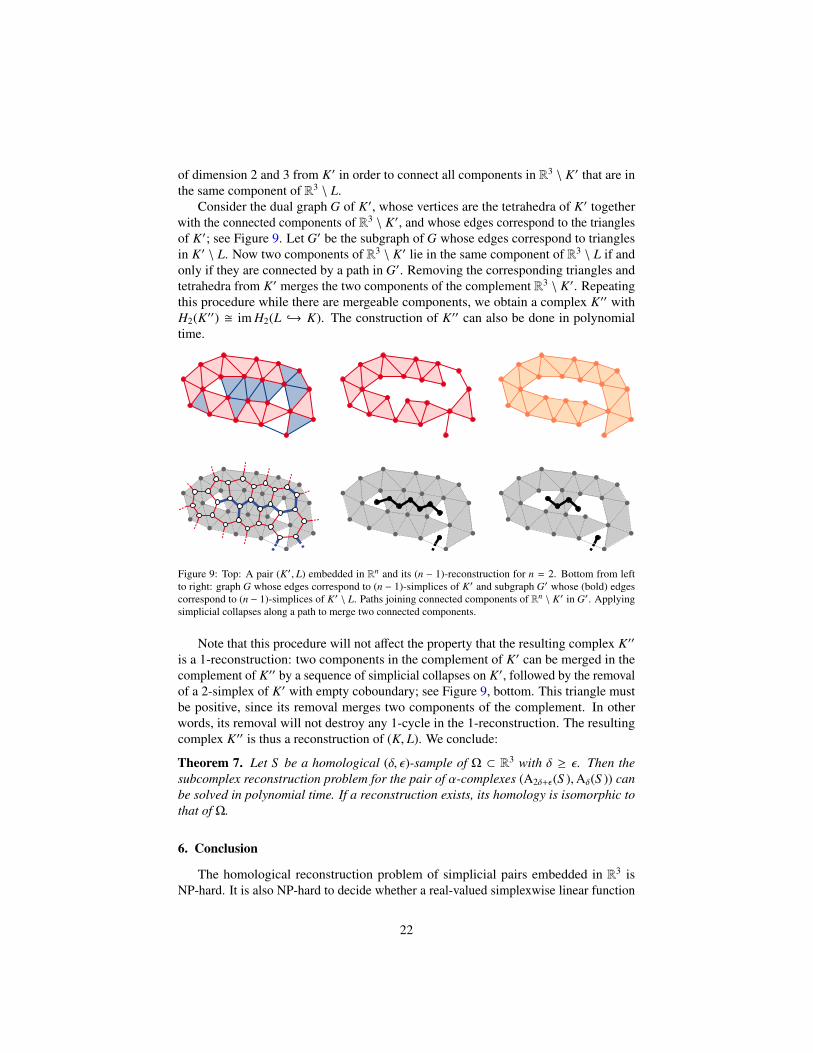
Consider the dual graph G of K0, whose vertices are the tetrahedra of K0 togetherwith the connected components of R3 \ K0, and whose edges correspond to the trianglesof K0; see Figure 9. Let G0 be the subgraph of G whose edges correspond to trianglesin K0 \ L. Now two components of R3 \ K0 lie in the same component of R3 \ L if andonly if they are connected by a path in G0. Removing the corresponding triangles andtetrahedra from K0 merges the two components of the complement R3 \ K0. Repeatingthis procedure while there are mergeable components, we obtain a complex K00 withH2(K00) � im H2(L ,! K). The construction of K00 can also be done in polynomialtime.

Figure 9: Top: A pair (K0, L) embedded in Rn and its (n � 1)-reconstruction for n = 2. Bottom from leftto right: graph G whose edges correspond to (n � 1)-simplices of K0 and subgraph G0 whose (bold) edgescorrespond to (n � 1)-simplices of K0 \ L. Paths joining connected components of Rn \ K0 in G0. Applyingsimplicial collapses along a path to merge two connected components.

Note that this procedure will not a↵ect the property that the resulting complex K00is a 1-reconstruction: two components in the complement of K0 can be merged in thecomplement of K00 by a sequence of simplicial collapses on K0, followed by the removalof a 2-simplex of K0 with empty coboundary; see Figure 9, bottom. This triangle mustbe positive, since its removal merges two components of the complement. In otherwords, its removal will not destroy any 1-cycle in the 1-reconstruction. The resultingcomplex K00 is thus a reconstruction of (K, L). We conclude:

Theorem 7. Let S be a homological (�, ✏)-sample of ⌦ ⇢ R3 with � � ✏. Then thesubcomplex reconstruction problem for the pair of ↵-complexes (A2�+✏(S ),A�(S )) canbe solved in polynomial time. If a reconstruction exists, its homology is isomorphic tothat of ⌦.

6. Conclusion

The homological reconstruction problem of simplicial pairs embedded in R3 isNP-hard. It is also NP-hard to decide whether a real-valued simplexwise linear function

22

in R3 has a level set or a sublevel set reconstruction. We deduce that simplifying thehomology of a simplicial pair embedded in R3 is also NP-hard and so is the homologicalsimplification of level and sublevel sets of real-valued simplexwise linear functionsin R3. On the other hand, such problems can be solved in polynomial time if werestrict ourselves to pairs of ↵-complexes in R3 that admit homological inference of acompact space, given an appropriate sample. Can we use this construction to devise ashape reconstruction algorithm with homological guarantees under the same samplingconditions?

Acknowledgements. This work was initiated during the 10th McGill–INRIA Workshopon Computational Geometry at the Bellairs Research Institute. The authors wish to thankall the participants for creating a pleasant and stimulating atmosphere, in particularNina Amenta for discussions leading to a first version of Theorem 1. Some of theauthors were partially supported by the GIGA ANR grant (contract ANR-09-BLAN-0331-01), the European project CG-Learning (contract 255827), and the Toposys projectFP7-ICT-318493-STREP.

[1] D. Attali and A. Lieutier. Optimal reconstruction might be hard. Discrete &Computational Geometry, 49(2):133–156, 2013.

[2] D. Attali, A. Lieutier, and D. Salinas. Vietoris–Rips complexes also providetopologically correct reconstructions of sampled shapes. Computational Geometry,46(4):448–465, 2013.

[3] P. Bendich, H. Edelsbrunner, D. Morozov, and A. Patel. Homology and robustnessof level and interlevel sets. Homology, Homotopy and Applications, 15(1):51–72,2013.

[4] P. Bubenik and J. Scott. Categorification of persistent homology. Discrete &Computational Geometry, 2014. Available online.

[5] F. Chazal and A. Lieutier. Stability and computation of topological invariants ofsolids in Rn. Discrete and Computational Geometry, 37(4):601–617, 2007.

[6] F. Chazal and A. Lieutier. Smooth manifold reconstruction from noisy and non-uniform approximation with guarantees. Computational Geometry, 40(2):156–170,2008.

[7] F. Chazal, D. Cohen-Steiner, and A. Lieutier. A sampling theory for compact setsin Euclidean space. Discrete & Computational Geometry, 41(3):461–479, 2009.

[8] F. Chazal, V. de Silva, M. Glisse, and S. Oudot. The structure and stability ofpersistence modules. Preprint, 2012. arXiv:1207.3674.

[9] D. Cohen-Steiner, H. Edelsbrunner, and D. Morozov. Vines and vineyards byupdating persistence in linear time. In Proceedings of the Twenty-second AnnualSymposium on Computational Geometry, SCG ’06, pages 119–126. ACM, 2006.

[10] D. Cohen-Steiner, H. Edelsbrunner, and J. Harer. Stability of persistence diagrams.Discrete & Computational Geometry, 37(1):103–120, 2007.

23

[11] D. Cohen-Steiner, H. Edelsbrunner, and J. Harer. Extending persistence usingPoincaré and Lefschetz duality. Foundations of Computational Mathematics, 9(1):79–103, 2008.

[12] V. de Silva and G. Carlsson. Topological estimation using witness complexes. InEurographics Symposium on Point-Based Graphics, pages 157–166, 2004.

[13] H. Edelsbrunner. Alpha shapes — a survey. In R. van de Weygaert, G. Vegter,J. Ritzerveld, and V. Icke, editors, Tessellations in the Sciences: Virtues, Techniquesand Applications of Geometric Tilings. Springer Verlag. To appear.

[14] H. Edelsbrunner and M. Kerber. Alexander duality for functions: the persistentbehavior of land and water and shore. In Proceedings of the 2012 symposium onComputational Geometry, pages 249–258. ACM, 2012.

[15] H. Edelsbrunner, D. Letscher, and A. Zomorodian. Topological persistence andsimplification. Discrete & Computational Geometry, 28(4):511–533, 2002.

[16] H. Edelsbrunner, D. Morozov, and A. Patel. Quantifying transversality by measur-ing the robustness of intersections. Foundations of Computational Mathematics,11(3):345–361, 2011.

[17] A. Hatcher. Algebraic Topology. Cambridge University Press, 2002.

[18] W. Kühnel. Triangulations of manifolds with few vertices. In F. Tricerri, editor,Advances in di↵erential geometry and topology, pages 59–114. World Scientific,Singapore, 1990.

[19] N. Milosavljevic, D. Morozov, and P. Skraba. Zigzag persistent homology in matrixmultiplication time. In Proceedings of the twenty-seventh annual symposium onComputational geometry, SoCG ’11, pages 216–225. ACM, 2011.

[20] D. Morozov. Homological Illusions of Persistence and Stability. PhD thesis, DukeUniversity, 2008.

[21] P. Niyogi, S. Smale, and S. Weinberger. Finding the homology of submanifoldswith high confidence from random samples. Discrete & Computational Geometry,39(1-3):419–441, 2008.

[22] E. H. Spanier. Algebraic Topology. Springer, 1994.

24