household wealth and resilience to financial shocks in italy

Household Wealth and Resilience toFinancial Shocks in Italy∗

Daniel Garcia-MaciaInternational Monetary Fund

Financial shocks in a sector of the economy transmit toother sectors via financial linkages. This paper constructs thematrix of bilateral financial sectoral exposures in Italy overthe last two decades. Using this information, it develops amethod to simulate how each sector absorbs plausible financialshocks. A fall in the value of government bonds directly affectsbanks and indirectly affects households via equity holdings inbanks. A bank bail-in is absorbed by foreigners and by house-holds, particularly those at the top of the wealth distribution.Conversely, in a bank bailout these two groups benefit from agovernment transfer.

JEL Codes: G11, G32, G33.

1. Introduction

Italian household wealth is high by international standards. Totalnet household wealth at end-2013 was estimated at over €9 trillion,or 51/2 times gross domestic product (GDP). Average wealth perhousehold exceeds €350,000 and per capita is about €150,000 (Bankof Italy 2014). As a percent of disposable income, it is higher than inmost euro-area peers, including Austria, Finland, France, Germany,

∗This paper benefited from comments by Majid Bazarbash, Rishi Goyal,Valentina Michelangeli, Diarmuid Murphy, Mahmood Pradhan, Mehdi Raissi,Concetta Rondinelli, Miguel Segoviano, one anonymous referee, and other col-leagues at seminars at the Bank of Italy and the IMF. David Velazquez-Romeroprovided research assistance. The views expressed herein are those of the authorand do not necessarily represent the views of the IMF, its Executive Board,or IMF management. Author contact: International Monetary Fund, EuropeanDepartment, 700 19th St NW, Washington, DC 20431. E-mail: [email protected].

241

242 International Journal of Central Banking September 2021

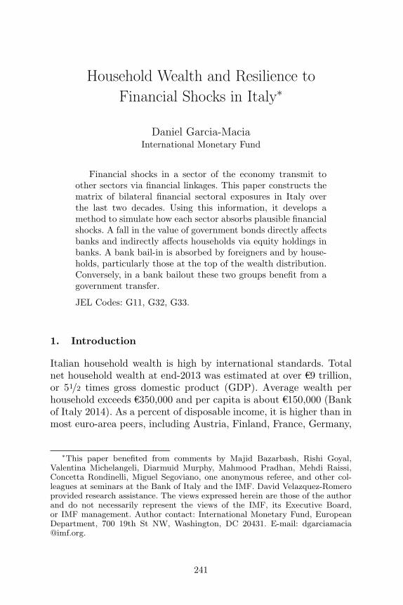
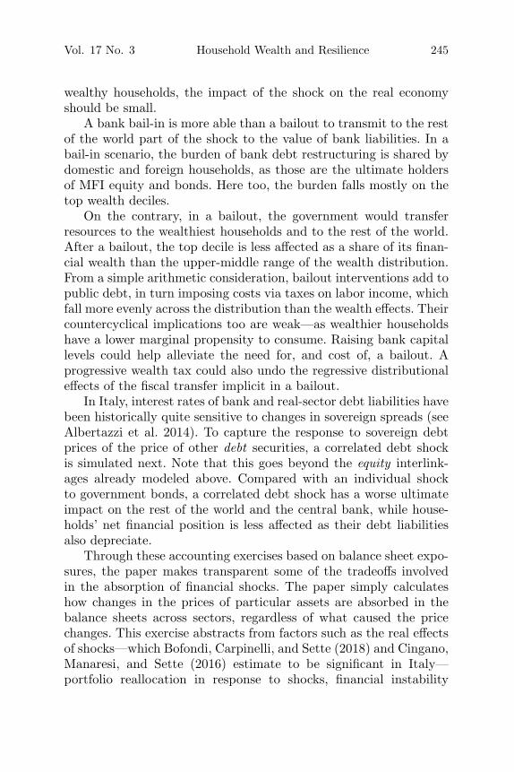
Figure 1. Average Net Wealth per Householdby Wealth Decile, 2014

Notes: The left panel shows net wealth per decile divided by the average grossincome across deciles. The dats are from the ECB Household Finance and Con-sumption Survey.

or Luxembourg. The middle and upper segments of the distribu-tion are particularly wealthy compared with the euro-area average,both as a share of income and in absolute terms (figure 1). Realassets—principally dwellings—constitute almost two-thirds of totalnet wealth, while financial assets are mostly concentrated in cashand deposits, shares, and insurance reserves.

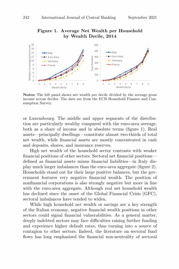
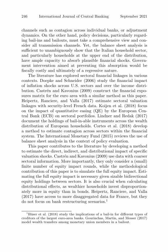
High net wealth of the household sector contrasts with weakerfinancial positions of other sectors. Sectoral net financial positions—defined as financial assets minus financial liabilities—in Italy dis-play much larger imbalances than the euro-area aggregate (figure 2).Households stand out for their large positive balances, but the gov-ernment features very negative financial wealth. The position ofnonfinancial corporations is also strongly negative but more in linewith the euro-area aggregate. Although real net household wealthhas declined since the onset of the Global Financial Crisis (GFC),sectoral imbalances have tended to widen.

While high household net wealth or savings are a key strengthof the Italian economy, negative financial wealth positions in othersectors could signal financial vulnerabilities. As a general matter,deeply indebted sectors may face difficulties raising further fundingand experience higher default rates, thus turning into a source ofcontagion to other sectors. Indeed, the literature on sectoral fundflows has long emphasized the financial non-neutrality of sectoral

Vol. 17 No. 3 Household Wealth and Resilience 243

Figure 2. Net Financial Assets by Sector(percent of GDP)

Notes: “NFCs” denotes nonfinancial corporations, “Government” is the generalgovernment, and “Other” includes the rest of the world and the financial sector:monetary and financial institutions, other financial institutions, insurance com-panies, and pension funds. The combined height of the bars shows the position inItaly. The figures on the bars indicate the difference between Italy and the euroarea. The data are from the Bank of Italy.

limits (e.g., Poterba 1987 documents the lack of a “corporate veil”).Understanding the transmission of shocks across sectors and theirultimate impact on households requires information about the inter-sectoral bilateral financial linkages. Shocks to the value of a giveninstrument issued by a given sector transmit to other sectors viadirect asset exposures and via equity interlinkages. For example, afall in the value of corporate debt can directly affect financial insti-tutions holding that debt, and in turn transmit to households withclaims on those financial institutions.

This paper constructs the matrix of bilateral financial sectoralexposures and simulates the impact of a series of illustrative finan-cial shocks. Instrument-level intersectoral financial positions areinferred from the Bank of Italy’s flow-of-funds data. The informa-tion on financial exposures is then illustratively used to infer the net


financial impact across sectors of a 10 percent fall in the value ofgovernment bonds, equivalent to a two-standard-deviation changein sovereign spreads, and of a 10 percent fall in the value of bankliabilities (i.e., the assets held by other sectors in banks), equiva-lent to the combined liabilities of the third and fourth Italian banks.The shock to bank liabilities is successively modeled as leading toeither a bail-in or a bailout. Household wealth survey data allow usto pin down the impact of these shocks across the household wealthdistribution.

The matrix of bilateral exposures reveals that, since 1995, house-hold wealth has been increasingly kept in insurance and pension fundassets and abroad. Households’ direct exposure to the governmenthas declined, although it is now intermediated by financial institu-tions. Government liabilities have been increasingly funded by therest of the world and financial institutions, with an important con-tribution from the Bank of Italy in recent years, reflecting the ECB’squantitative easing. However, international financial diversificationof Italian residents has slowed down. Since the GFC, nonfinancialcorporate balance sheets have shrunk, with households being thesector that has reduced more its investment.

Within the household sector, the distribution of financial expo-sures is related to wealth levels. According to the Survey on House-hold Income and Wealth of the Bank of Italy, financial wealth and,in particular, risky assets are concentrated at the upper end ofthe distribution. The top two household wealth deciles accumulatemore than two-thirds of financial wealth and an even larger pro-portion of equity and nonsecured debt. Less wealthy householdsown almost all their financial wealth in the form of insured bankdeposits.

Given the bilateral instrument-level exposures, a fall in the valueof government bonds is estimated to directly affect the financial sec-tor and indirectly households. The Bank of Italy, private monetaryfinancial institutions (MFIs, mostly banks), insurance and pensionfunds, and the rest of the world bear sizable balance sheet losses.However, as private financial institutions are ultimately owned byother sectors, primarily domestic and foreign households, thesehouseholds—especially at the upper end of the wealth distribution—bear the brunt of the losses. Given the healthy financial position ofhouseholds, together with the concentration of financial assets in


wealthy households, the impact of the shock on the real economyshould be small.

A bank bail-in is more able than a bailout to transmit to the restof the world part of the shock to the value of bank liabilities. In abail-in scenario, the burden of bank debt restructuring is shared bydomestic and foreign households, as those are the ultimate holdersof MFI equity and bonds. Here too, the burden falls mostly on thetop wealth deciles.

On the contrary, in a bailout, the government would transferresources to the wealthiest households and to the rest of the world.After a bailout, the top decile is less affected as a share of its finan-cial wealth than the upper-middle range of the wealth distribution.From a simple arithmetic consideration, bailout interventions add topublic debt, in turn imposing costs via taxes on labor income, whichfall more evenly across the distribution than the wealth effects. Theircountercyclical implications too are weak—as wealthier householdshave a lower marginal propensity to consume. Raising bank capitallevels could help alleviate the need for, and cost of, a bailout. Aprogressive wealth tax could also undo the regressive distributionaleffects of the fiscal transfer implicit in a bailout.

In Italy, interest rates of bank and real-sector debt liabilities havebeen historically quite sensitive to changes in sovereign spreads (seeAlbertazzi et al. 2014). To capture the response to sovereign debtprices of the price of other debt securities, a correlated debt shockis simulated next. Note that this goes beyond the equity interlink-ages already modeled above. Compared with an individual shockto government bonds, a correlated debt shock has a worse ultimateimpact on the rest of the world and the central bank, while house-holds’ net financial position is less affected as their debt liabilitiesalso depreciate.

Through these accounting exercises based on balance sheet expo-sures, the paper makes transparent some of the tradeoffs involvedin the absorption of financial shocks. The paper simply calculateshow changes in the prices of particular assets are absorbed in thebalance sheets across sectors, regardless of what caused the pricechanges. This exercise abstracts from factors such as the real effectsof shocks—which Bofondi, Carpinelli, and Sette (2018) and Cingano,Manaresi, and Sette (2016) estimate to be significant in Italy—portfolio reallocation in response to shocks, financial instability


channels such as contagion across individual banks, or adjustmentdynamics. On the other hand, policy decisions, particularly regard-ing bail-ins and bailouts, must take a comprehensive view and con-sider all transmission channels. Yet, the balance sheet analysis issufficient to unambiguously show that the Italian household sector,and particularly households at the upper end of the distribution,have ample capacity to absorb plausible financial shocks. Govern-ment intervention aimed at preventing this absorption would befiscally costly and ultimately of a regressive nature.

The literature has explored sectoral financial linkages in variouscontexts. Doepke and Schneider (2006) study the financial impactof inflation shocks across U.S. sectors and over the income distri-bution. Castren and Kavonius (2009) construct the financial expo-sures matrix for the euro area with a similar method as this paper.Heipertz, Ranciere, and Valla (2017) estimate sectoral valuationlinkages with security-level French data. Koijen et al. (2018) focuson the impact of quantitative easing (QE) by the European Cen-tral Bank (ECB) on sectoral portfolios. Lindner and Redak (2017)document the holdings of bail-in-able instruments across the wealthdistribution of European households. Cortes et al. (2018) developa method to estimate contagion across sectors within the financialsystem. The International Monetary Fund (2015) reviews the use ofbalance sheet analysis in the context of policy evaluation.

This paper contributes to the literature by developing a methodto estimate the direct, indirect, and distributional impact of specificvaluation shocks. Castren and Kavonius (2009) use data with coarsersectoral information. More importantly, they only consider a (small)finite number of equity impact rounds, while the methodologicalcontribution of this paper is to simulate the full equity impact. Esti-mating the full equity impact is necessary given sizable bidirectionalequity holdings between sectors. It is also crucial when calculatingdistributional effects, as wealthier households invest disproportion-ately more in equity than in bonds. Heipertz, Ranciere, and Valla(2017) have access to more disaggregated data for France, but theydo not focus on bank restructuring scenarios.1

1Huser et al. (2018) study the implications of a bail-in for different types ofcreditors of the largest euro-area banks. Gourinchas, Martin, and Messer (2017)model wealth transfers among monetary union members in a bailout.


The rest of the paper is organized as follows. Section 2 describesthe data and the accounting method. Section 3 documents finan-cial exposures in Italy. Section 4 describes the method to simulatethe impact of financial shocks. Section 5 presents the results of thesimulation. Section 6 analyzes the distributional impact of financialshocks. Section 7 concludes.

2. Data and Accounting Method

Flow-of-funds data provide information on sectoral financial expo-sures. The Bank of Italy publishes quarterly flow-of-funds data(sourced via Haver) covering the period 1995:Q1–2017:Q3. This dataset contains information, for each economic sector, on the stockpositions in different financial instruments (assets and liabilities).2

Table 1 lists the disaggregation of sectors in the data as well as thesimplified grouping applied in this paper.

The data are used to construct a matrix of cross-sectoral bilat-eral financial exposures. A given entry (i, j) in the matrix containsthe financial asset holdings of sector i invested in sector j, or equiva-lently the liabilities of sector j with respect to sector i. Appendix Adescribes the steps and necessary assumptions to infer bilateral sec-toral exposures from the Italian flow-of-funds data. The data set onlyincludes financial assets. A sector can have a nonzero net financialasset balance, which should be matched by an opposite net balanceof real assets or by own-sector net worth (in the case of BOI, GOV,HH, and RoW).

Survey data allow us to zoom in to household financial expo-sures as a function of household wealth. The Bank of Italy’s Surveyon Household Income and Wealth (2016 release) contains finan-cial information (and sample weights) for a representative sampleof about 7,000 households. These data are used to calculate thedistribution of stock positions and the impact of financial shocksacross household wealth deciles. The ECB’s Household Finance andConsumption Survey (2014 release) allows us to compare with thedistribution in other euro-area economies.

2The classification follows the European System of Accounts (ESA) for 2010.


Table 1. Grouping of Sectors

Original Sectors in the Data Coding

Nonfinancial Corporations NFC

Monetary Financial Institutions Excluding MFICentral Bank

Bank of Italy BOI

Other Financial Intermediaries Excluding OFINon-MMF Investment Funds

Non-MMF Investment FundsFinancial Auxiliaries

Insurance Companies INPPension Funds

Central Government GOVLocal GovernmentSocial Security Funds

Households and Nonprofit Institutions HHServing Households

Rest of the World RoW

3. Sectoral Financial Exposures in Italy

Table 2 contains the matrix of sectoral financial exposures in Italy in2017:Q3, expressed as a percent of GDP. For example, nonfinancialcorporates (NFCs) own financial assets of monetary financial insti-tutions (MFIs) worth 14 percent of GDP, and equivalently MFIshave financial liabilities of 14 percent of GDP with respect to NFCs.The rightmost column shows the net financial asset (NFA) positionof each sector, equal to total assets minus total liabilities.3

The distribution of sectoral financial linkages is highly non-uniform. Table 2 shows that NFCs have a very negative NFA

3Summing up all sectors, total financial assets equal total financial liabilities,i.e., the system is closed, as it includes the position of the rest of the worldvis-a-vis Italy.


Table 2. Sectoral Financial Asset Exposures, 2017:Q3(percent of GDP)

NFC MFI BOI OFI INP GOV HH RoW Tot. As. NFA

NFC 14 7 1 2 6 5 27 61 −112MFI 54 5 13 1 37 37 23 170 0BOI 0 16 0 0 22 0 13 53 6OFI 11 18 2 0 8 4 26 69 27INP 4 3 1 3 20 0 25 55 −2GOV 11 5 1 4 1 4 4 30 −124HH 54 64 19 16 50 14 30 247 196RoW 39 50 12 6 3 47 1 157 8Tot. Liab. 174 170 47 42 56 154 51 149 843

Notes: Rows indicate the creditor sector and columns indicate the debtor sector. Rows sum tototal assets and columns to total liabilities. NFA: net financial assets. The source data are fromthe Bank of Italy.

position, with liabilities mainly to MFIs and households. The mirrorimage is the extremely positive NFA of households, with assets pre-dominantly in MFIs, NFCs, and insurance and pension funds (in thisorder). The government is very indebted, mostly due to the financialsector and the rest of the world. The Bank of Italy is an importantcreditor of the government, reflecting the Eurosystem’s implemen-tation of QE via its local branch. However, the public sector alsoholds a significant amount of assets in private sectors, especiallyNFCs, suggesting it has room to divest and cut its gross liabilities.MFIs are (not surprisingly) financially balanced, with assets in NFCsand the government, and liabilities to households and the rest of theworld.

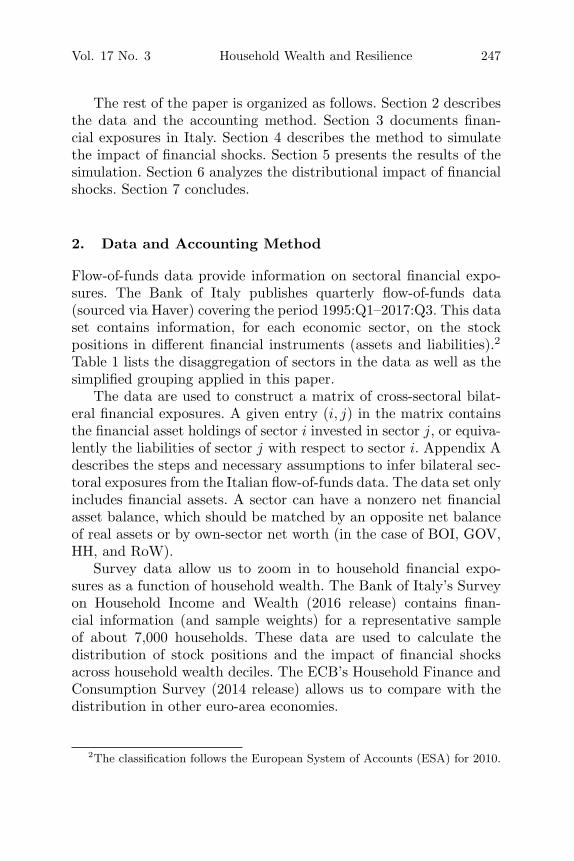
The portfolio composition is visualized in table 3, which expressesfinancial exposures as a share of total sector assets. This nets outthe effect of a sector’s balance sheet size. One key message is thatMFIs and insurance and pension funds are relatively more exposedto government assets, which indirectly exposes their creditors and/orshareholders, such as households and NFCs.

Next, the evolution of sectoral exposures over five data snap-shots is explored. These snapshots are (i) the beginning of the sam-ple, 1995:Q1; (ii) the deployment of the euro, 2001:Q4; (iii) theonset of the GFC, 2008:Q1; (iv) the Outright Monetary Trans-actions program announcement, 2012:Q2; and (v) the end of the


Table 3. Sectoral Financial Asset Exposures, 2017:Q3(percent of sector assets)

NFC MFI BOI OFI INP GOV HH RoW Total

NFC 23 11 2 3 10 9 43 100MFI 32 3 7 1 22 22 14 100BOI 1 31 1 0 42 0 25 100OFI 16 27 3 0 11 6 37 100INP 7 5 1 5 36 0 46 100GOV 36 17 3 12 2 14 15 100HH 22 26 8 6 20 6 12 100RoW 25 32 8 4 2 30 1 100All 21 20 6 5 7 18 6 18 100

Notes: The last row shows the portfolio composition for the aggregate of all sectors.The source data are from the Bank of Italy.

sample, 2017:Q3. Appendix B contains the full matrix of bilat-eral exposures at each point in time, while figure 3 reports keytakeaways.

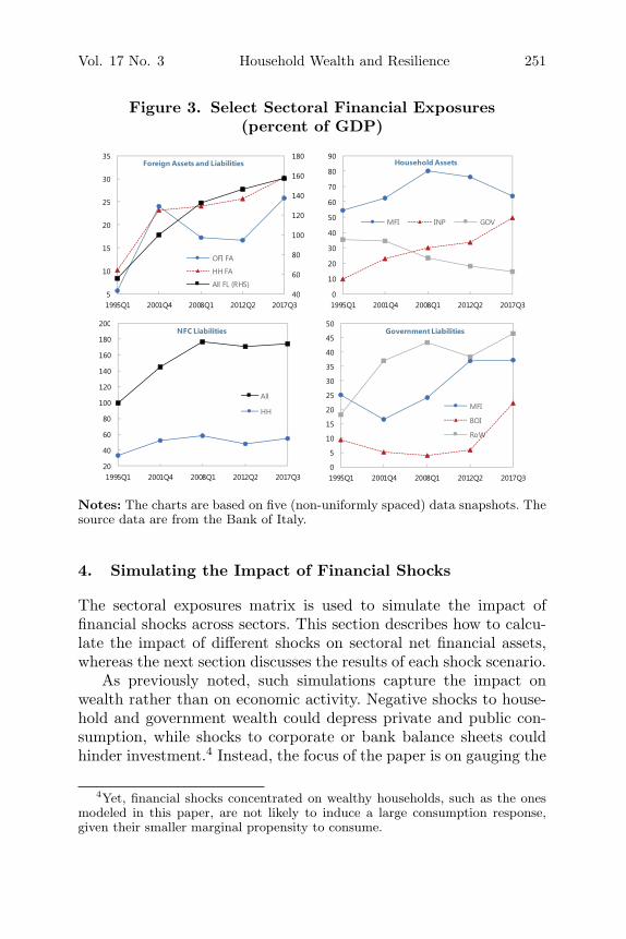
The sum of financial assets in all sectors doubled from 1995:Q1 to2017:Q3 (from 418 to 843 percent of GDP). This reflects the processof European financial integration as well as the increase in financialintermediation. The first panel of figure 3 shows the growing impor-tance of foreign liabilities as well as the diversification of house-holds and other financial institutions (OFIs) toward foreign assetholdings, peaking at the time of euro accession. Yet, the diversifica-tion process has slowed down, and the degree of home bias remainselevated.

The second panel shows that households shifted their asset port-folio away from the government and into insurance and pensionfunds. Their asset holdings in MFIs peaked in the run-up to theGFC but receded thereafter. The GFC also halted the accumulationof NFC liabilities, mostly due to a decline in household investment.On the other hand, the government became more reliant on MFIfunding after the GFC, when some international creditors retreated.Since 2012, the Bank of Italy stepped in as a major creditor throughthe implementation of monetary policy.


Figure 3. Select Sectoral Financial Exposures(percent of GDP)

Notes: The charts are based on five (non-uniformly spaced) data snapshots. Thesource data are from the Bank of Italy.

4. Simulating the Impact of Financial Shocks

The sectoral exposures matrix is used to simulate the impact offinancial shocks across sectors. This section describes how to calcu-late the impact of different shocks on sectoral net financial assets,whereas the next section discusses the results of each shock scenario.

As previously noted, such simulations capture the impact onwealth rather than on economic activity. Negative shocks to house-hold and government wealth could depress private and public con-sumption, while shocks to corporate or bank balance sheets couldhinder investment.4 Instead, the focus of the paper is on gauging the

4Yet, financial shocks concentrated on wealthy households, such as the onesmodeled in this paper, are not likely to induce a large consumption response,given their smaller marginal propensity to consume.


households’ shock or loss-absorption capacity, given its importancefor financial stability in Italy. Moreover, for simplicity, the simu-lations abstract from potential correlated price changes in othersecurities—beyond the change in equity values, portfolio realloca-tion after the shocks (e.g., prompted by regulatory constraints), oradjustment dynamics.

4.1 Valuation Shock

4.1.1 One Instrument in One Sector

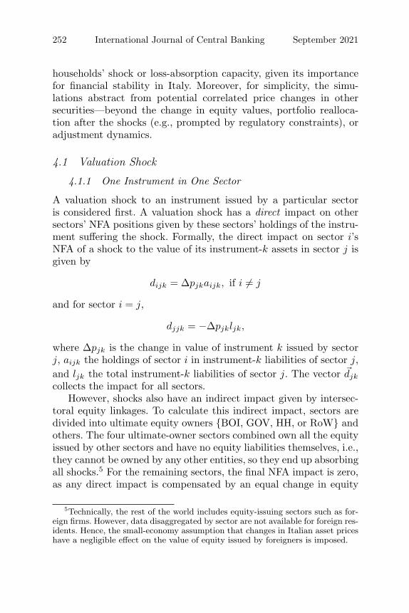
A valuation shock to an instrument issued by a particular sectoris considered first. A valuation shock has a direct impact on othersectors’ NFA positions given by these sectors’ holdings of the instru-ment suffering the shock. Formally, the direct impact on sector i’sNFA of a shock to the value of its instrument-k assets in sector j isgiven by

dijk = Δpjkaijk, if i �= j

and for sector i = j,

djjk = −Δpjkljk,

where Δpjk is the change in value of instrument k issued by sectorj, aijk the holdings of sector i in instrument-k liabilities of sector j,and ljk the total instrument-k liabilities of sector j. The vector �djk

collects the impact for all sectors.However, shocks also have an indirect impact given by intersec-

toral equity linkages. To calculate this indirect impact, sectors aredivided into ultimate equity owners {BOI, GOV, HH, or RoW} andothers. The four ultimate-owner sectors combined own all the equityissued by other sectors and have no equity liabilities themselves, i.e.,they cannot be owned by any other entities, so they end up absorbingall shocks.5 For the remaining sectors, the final NFA impact is zero,as any direct impact is compensated by an equal change in equity

5Technically, the rest of the world includes equity-issuing sectors such as for-eign firms. However, data disaggregated by sector are not available for foreign res-idents. Hence, the small-economy assumption that changes in Italian asset priceshave a negligible effect on the value of equity issued by foreigners is imposed.


liabilities to either HH, GOV, BOI, or RoW. Of course, this is notto say that financial shocks are without consequences for the non-ultimate-owner sectors, which may suffer from lower profitability,higher funding costs, default or restructuring events, market runs,and/or regulatory pressure.

Formally, the calculation involves two steps. First, the interme-diate equity impact e′ among the non-absorber sectors is

e′ijk = (I − M)−1

∑s={NFC,MFI,OFI,INP}

dsjkE′is,

if i = {NFC, MFI, OFI, INP} ,

where I is the identity matrix,

M ≡ E′ − diag (E′) − λ (E′ − diag (E′)) I,

λ is a vector of ones, and E′ is a matrix showing the fraction ofsector s’s equity owned by sector i if i �= s and equal to the resid-ual share otherwise, defined for i = {NFC, MFI, OFI, INP}.6 Thematrix M captures the difference between a sector’s equity holdingsin other sectors (off-diagonal entries) and its equity liabilities (diag-onal entries). The geometric-sum term (I − M)−1 reflects the infi-nite rounds of knock-on effects across sectors interlinked by mutualequity exposures.

Second, the ultimate equity impact e for the shock absorbers iscalculated as

eijk =∑

s={NFC,MFI,OFI,INP}e′sjkEis, if i = {BOI, GOV, HH, RoW},

where E is a matrix showing the fraction of sector s’sequity owned by sector i, imposing zero ownership for i ={NFC, MFI, OFI, INP

}.7

6Equity positions include both the ESA category “shares and other equity”and the fraction of non-money-market mutual fund positions which are investedin shares and other equity: 15 percent.

7Given the lack of perfect sector-by-sector disaggregation in the data, non-absorption by i = {NFC, MFI, OFI, NPI} must be imposed as a constraint inthe calculation.


For the non-absorber sectors, the equity impact is simply theopposite of the direct impact:

eijk = −dijk, if i = {NFC, MFI, OFI, NPI} ,

which makes the total impact zero, as discussed above.The total NFA impact across sectors is the sum of the direct and

indirect impact of the shock:

ΔNFA = �djk + �ejk.

4.1.2 Multiple Instruments and Sectors

Generalizing the formulas to account for shocks to the prices of mul-tiple instruments or sectors is straightforward. The direct impact forinstrument k held by sector i becomes

dijk =∑

s∈{S}\j

Δpskaisk − Δpiklik,

where S represents the subset of issuer sectors experiencing a pricechange in instrument k.

If price changes occur in multiple instruments, the direct impactcan be simply added up. The formulas for the equity and totalimpacts are as for the case with one instrument in one sector above.

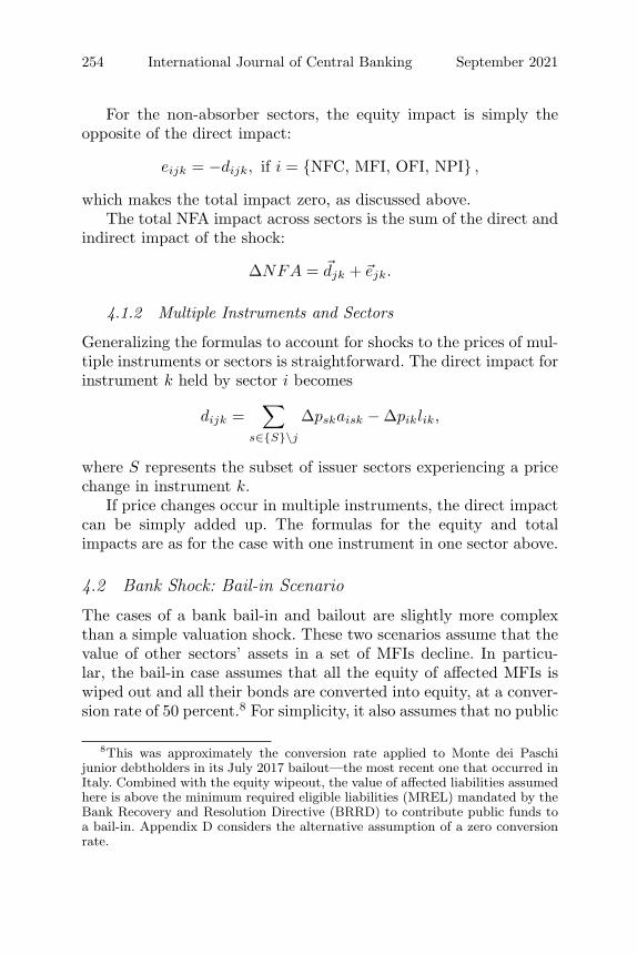
4.2 Bank Shock: Bail-in Scenario

The cases of a bank bail-in and bailout are slightly more complexthan a simple valuation shock. These two scenarios assume that thevalue of other sectors’ assets in a set of MFIs decline. In particu-lar, the bail-in case assumes that all the equity of affected MFIs iswiped out and all their bonds are converted into equity, at a conver-sion rate of 50 percent.8 For simplicity, it also assumes that no public

8This was approximately the conversion rate applied to Monte dei Paschijunior debtholders in its July 2017 bailout—the most recent one that occurred inItaly. Combined with the equity wipeout, the value of affected liabilities assumedhere is above the minimum required eligible liabilities (MREL) mandated by theBank Recovery and Resolution Directive (BRRD) to contribute public funds toa bail-in. Appendix D considers the alternative assumption of a zero conversionrate.


resolution funds are used and that other (nonbond) debtholders arenot affected.

The direct impact is given by the sum of the valuation changein MFI equity and bond liabilities times the exposure of each sectorto these two assets.

Since in a bail-in equity is wiped out, original shareholders do notbenefit from the reduction in bond liabilities, so there is no indirectequity impact for MFIs:

eijk = 0, if i = MFI.

For the rest of non-absorber sectors, the intermediate equity impactis

e′ijk = (I − M ′′)−1 ∑

s={NFC,OFI,INP}dsjkE′′

is, if i = {NFC, OFI, INP} ,

where E′′ and M ′′ are, respectively, defined like E′ and M but onlyfor sectors i = {NFC, OFI, INP}.

The ultimate equity impact for sectors other than MFIs is givenby the same formulas as in the valuation shock case above.

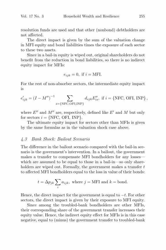
4.3 Bank Shock: Bailout Scenario

The difference in the bailout scenario compared with the bail-in sce-nario is the government’s intervention. In a bailout, the governmentmakes a transfer to compensate MFI bondholders for any losses—which are assumed to be equal to those in a bail-in—so only share-holders are wiped out. Formally, the government makes a transfer tto affected MFI bondholders equal to the loss in value of their bonds:

t = Δpjk

∑i

aijk, where j = MFI and k = bond.

Hence, the direct impact for the government is equal to −t. For othersectors, the direct impact is given by their exposure to MFI equity.

Since among the troubled-bank bondholders are other MFIs,their corresponding share of the government transfer increases theirequity value. Hence, the indirect equity effect for MFIs is in this casenegative, equal to (minus) the government transfer to troubled-bank


bondholder MFIs. Thus, the equity impact for MFIs can be calcu-lated as the difference between the bail-in direct impact and thebailout direct impact (as the former does not include the governmenttransfer, which is ultimately transmitted to MFI shareholders).

For the rest of non-absorber sectors,

e′ijk = (I − M)−1

∑s={NFC,MFI,OFI,INP}

d′sjkE′

is,

if i = {NFC, OFI, INP} ,

where d′sjk is equal to dsjk if s = {NFC, OFI, INP}, and it is equal

to minus the ultimate equity impact for MFIs if s = MFI.The ultimate equity impact for sectors other than MFIs is given

by the same formulas as in the valuation shock case.

5. Illustrative Shock Scenarios

5.1 Individual Shocks

This section presents results for a calibration of the three types ofindividual shocks dicussed above. A shock equivalent to a 10 percentdecline in the value of government bonds (e.g., due to an increasein market perception of risk or nominal interest rates) is consideredfirst.9 Table 4 shows that the direct impact, given by governmentbond exposures, is concentrated on the financial sector—includingMFIs, the Bank of Italy, and insurance and pension funds—as wellas on the rest of the world. However, once equity linkages are con-sidered, the sector with a larger total NFA decline is the rest of theworld, followed by households. The impact on households as a frac-tion of GDP is non-negligible at about 4 percent of GDP, but only 2percent as a fraction of their NFA. Government liabilities diminishby an equal amount, which raises the government’s NFA position.

9 This is equivalent to an increase in yields of around 220 basis points, given theduration of Italian outstanding government debt of 4.88 years (source: Bloomberg,as of May 2018), or a two-standard-deviation spread change, based on end-of-quarter year-on-year data for 1995:Q1–2018:Q3 (source: Reuters). For compari-son, this is about 1.5 times the increase Italy experienced in late May 2018, andthus an economically sizable shock. Since the analysis is purely static, there is noneed to specify the persistence of the shock.


Table 4. Impact of a Government Bond Value Shock(percent of GDP)

Direct EquityNFA Impact Impact ΔNFA

NFC −112 −0.3 0.3 0.0MFI 0 −2.1 2.1 0.0BOI 6 −2.2 0.0 −2.2OFI 27 −0.7 0.7 0.0INP −2 −2.0 2.0 0.0GOV −124 11.7 −0.4 11.3HH 196 −0.8 −3.1 −3.8RoW 8 −3.7 −1.6 −5.3

Notes: Assuming a 10 percent decline in the value of general government bonds.The direct impact on the NFA is given by the general government bond exposures.The equity impact is given by the bilateral equity linkages. ΔNFA is equal to directimpact plus the equity impact. The results are based on 2017:Q3 data from the Bankof Italy.

Next, a bank bail-in is compared with a bank bailout scenario.The two scenarios simulate a bank restructuring affecting a bank(or set of banks) constituting 10 percent of MFI liabilities, roughlyequivalent to the combined size of Italy’s third and fourth largestbanks (by assets). This implies a 10 percent reduction in the valueof MFI equity liabilities and a 5 percent reduction in the value oftheir bond liabilities (at a 50 percent conversion rate). In the caseof a bailout, bond losses are fully compensated by the government,as explained in the previous section.

Table 5 shows that a bank bail-in mostly affects households andthe rest of the world. This applies to both the direct and the totalNFA impact. In fact, almost half of a bail-in’s impact is absorbed bythe rest of the world, which should mitigate the shock’s damage tothe domestic real economy. The impact on households is slightly over1 percent of GDP, or 1/2 percent of the households’ NFA. The NFAof MFIs increases as their liabilities to other sectors are reduced.

A bailout is less successful in sharing the impact with the restof the world (table 6). The burden of a bailout falls mostly on thegovernment, at over 11/2 percent of GDP, which worsens an already


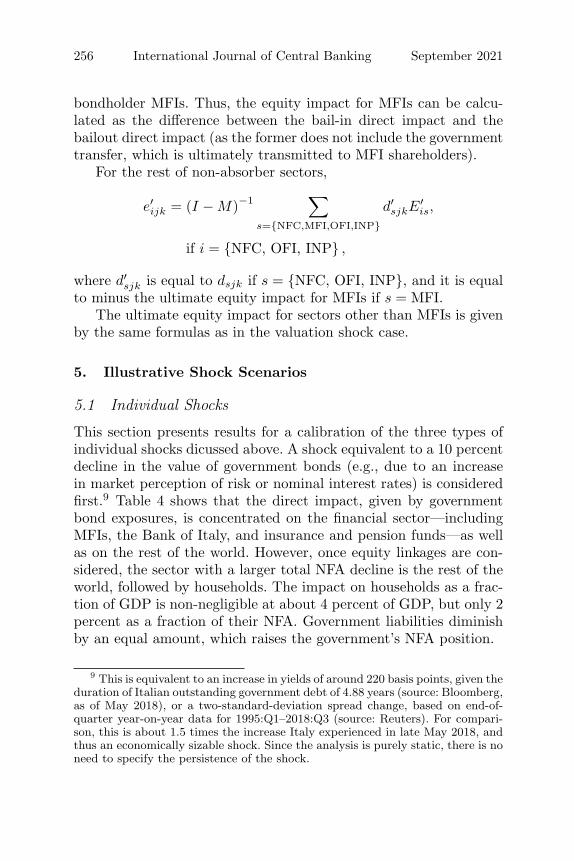
Table 5. Impact of a Bank Bail-In (percent of GDP)


NFC −112 −0.2 0.2 0.0MFI 0 2.3 0.0 2.3BOI 6 −0.1 0.0 −0.1OFI 27 −0.1 0.1 0.0INP −2 −0.1 0.1 0.0GOV −124 −0.1 0.0 −0.1HH 196 −0.9 −0.3 −1.2RoW 8 −0.7 −0.1 −0.9

Notes: Assuming banks constituting 10 percent of MFI assets are bailed in. All theirequity is wiped out and all their bonds converted to equity, at a 50 percent conversionrate. The results are based on 2017:Q3 data from the Bank of Italy.

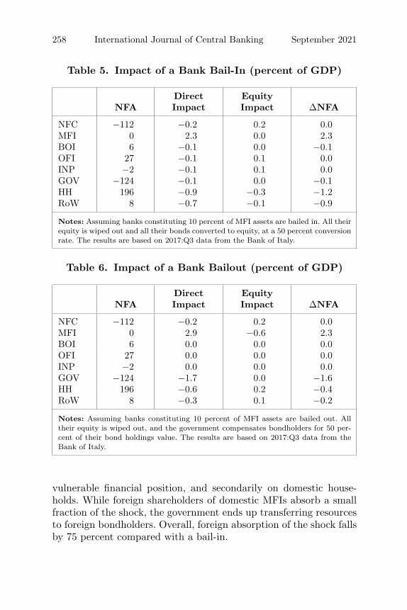
Table 6. Impact of a Bank Bailout (percent of GDP)


NFC −112 −0.2 0.2 0.0MFI 0 2.9 −0.6 2.3BOI 6 0.0 0.0 0.0OFI 27 0.0 0.0 0.0INP −2 0.0 0.0 0.0GOV −124 −1.7 0.0 −1.6HH 196 −0.6 0.2 −0.4RoW 8 −0.3 0.1 −0.2

Notes: Assuming banks constituting 10 percent of MFI assets are bailed out. Alltheir equity is wiped out, and the government compensates bondholders for 50 per-cent of their bond holdings value. The results are based on 2017:Q3 data from theBank of Italy.

vulnerable financial position, and secondarily on domestic house-holds. While foreign shareholders of domestic MFIs absorb a smallfraction of the shock, the government ends up transferring resourcesto foreign bondholders. Overall, foreign absorption of the shock fallsby 75 percent compared with a bail-in.


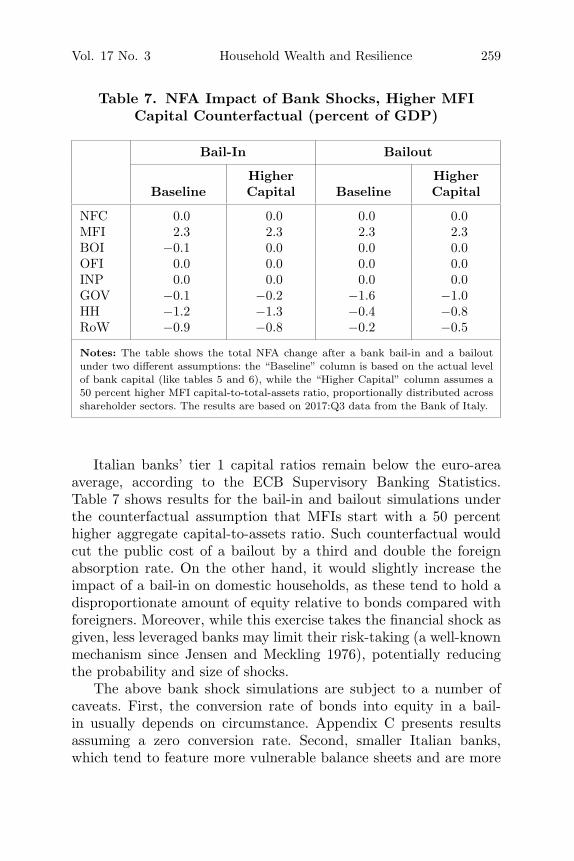
Table 7. NFA Impact of Bank Shocks, Higher MFICapital Counterfactual (percent of GDP)

Bail-In Bailout

Higher HigherBaseline Capital Baseline Capital

NFC 0.0 0.0 0.0 0.0MFI 2.3 2.3 2.3 2.3BOI −0.1 0.0 0.0 0.0OFI 0.0 0.0 0.0 0.0INP 0.0 0.0 0.0 0.0GOV −0.1 −0.2 −1.6 −1.0HH −1.2 −1.3 −0.4 −0.8RoW −0.9 −0.8 −0.2 −0.5

Notes: The table shows the total NFA change after a bank bail-in and a bailoutunder two different assumptions: the “Baseline” column is based on the actual levelof bank capital (like tables 5 and 6), while the “Higher Capital” column assumes a50 percent higher MFI capital-to-total-assets ratio, proportionally distributed acrossshareholder sectors. The results are based on 2017:Q3 data from the Bank of Italy.

Italian banks’ tier 1 capital ratios remain below the euro-areaaverage, according to the ECB Supervisory Banking Statistics.Table 7 shows results for the bail-in and bailout simulations underthe counterfactual assumption that MFIs start with a 50 percenthigher aggregate capital-to-assets ratio. Such counterfactual wouldcut the public cost of a bailout by a third and double the foreignabsorption rate. On the other hand, it would slightly increase theimpact of a bail-in on domestic households, as these tend to hold adisproportionate amount of equity relative to bonds compared withforeigners. Moreover, while this exercise takes the financial shock asgiven, less leveraged banks may limit their risk-taking (a well-knownmechanism since Jensen and Meckling 1976), potentially reducingthe probability and size of shocks.

The above bank shock simulations are subject to a number ofcaveats. First, the conversion rate of bonds into equity in a bail-in usually depends on circumstance. Appendix C presents resultsassuming a zero conversion rate. Second, smaller Italian banks,which tend to feature more vulnerable balance sheets and are more


likely to be restructured, are also disproportionately owned bydomestic households.10 Taking this into account would reduce thesubsidy to the rest of the world associated with a bailout. Third,unlike a bail-in, a bailout may prevent contagion to other MFIs,potentially preventing detrimental knock-on effects on financial sta-bility and investment. Finally, the bail-in and bailout scenarios mustbe interpreted as illustrative polar cases, since actual experiences ofbank restructuring typically contain elements of both.

5.2 Correlated Shock

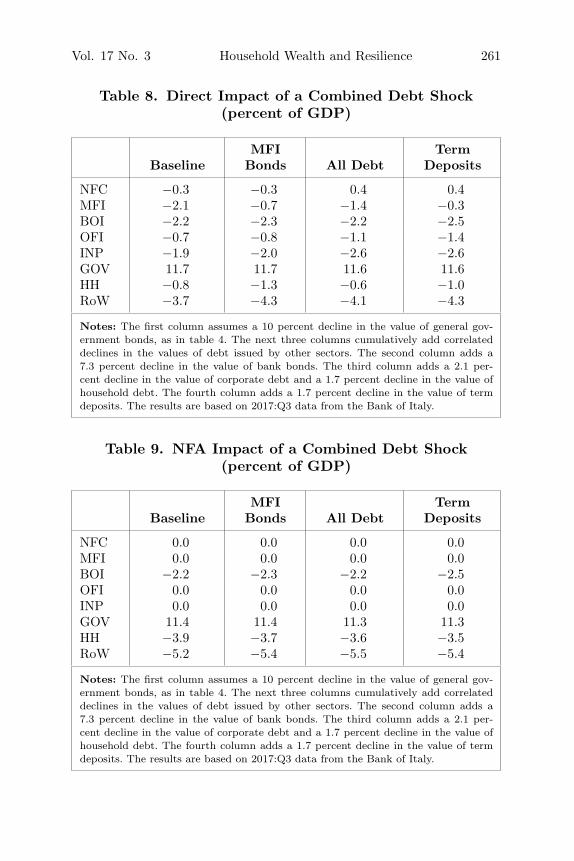
Shocks to the value of government debt in Italy tend to cause changesin the value of other debt securities. Albertazzi et al. (2014) esti-mate that a 100 basis point increase in spreads leads to a 73 basispoint increase in MFI bonds rates after one quarter, a 21 basis pointincrease in corporate credit rates, 17 basis points in household credit,and 34 basis points in MFI term deposits. Using these estimates ofthe correlation between government bond rates and other securities,tables 8 and 9 recalculate the direct and total NFA impact, respec-tively, of a shock to the value of government bonds.11 The tablesintroduce the correlations in a cumulative manner: the first columncorresponds to the table 4 baseline, the second column adds a cor-related response of bank bonds, the third column adds the responseof corporate and household credit, and the fourth term deposits.12

Focusing on the direct exposures (table 8), a depreciation of MFIbonds increases the impact for households and the rest of the world,while it obviously creates a valuation gain for MFIs. Adding a depre-ciation of debt securities by all sectors harms the financial sector,

10See SNL bank-level data showing lower capitalization and profitability inseveral banks outside the largest two.

11To translate interest rate correlations into price correlations, MFI bonds andprivate credit are both assumed to have similar average duration as governmentbonds, while MFI deposits are assumed to have half the duration. Data for MFIbond average maturity are available from Bloomberg, while data on outstandingamounts of other debt securities by broad maturity bins are available from Bankof Italy statistics.

12The order of addition is motivated by the experience during the 2018 sover-eign spread hike, when pass-through was strongest for bank bonds. In fact, the2018 response of credit and especially term deposit rates has been muted so far,suggesting the last two columns in tables 8 and 9 should be taken as an upperbound.


Table 8. Direct Impact of a Combined Debt Shock(percent of GDP)

MFI TermBaseline Bonds All Debt Deposits

NFC −0.3 −0.3 0.4 0.4MFI −2.1 −0.7 −1.4 −0.3BOI −2.2 −2.3 −2.2 −2.5OFI −0.7 −0.8 −1.1 −1.4INP −1.9 −2.0 −2.6 −2.6GOV 11.7 11.7 11.6 11.6HH −0.8 −1.3 −0.6 −1.0RoW −3.7 −4.3 −4.1 −4.3

Notes: The first column assumes a 10 percent decline in the value of general gov-ernment bonds, as in table 4. The next three columns cumulatively add correlateddeclines in the values of debt issued by other sectors. The second column adds a7.3 percent decline in the value of bank bonds. The third column adds a 2.1 per-cent decline in the value of corporate debt and a 1.7 percent decline in the value ofhousehold debt. The fourth column adds a 1.7 percent decline in the value of termdeposits. The results are based on 2017:Q3 data from the Bank of Italy.

Table 9. NFA Impact of a Combined Debt Shock(percent of GDP)

MFI TermBaseline Bonds All Debt Deposits

NFC 0.0 0.0 0.0 0.0MFI 0.0 0.0 0.0 0.0BOI −2.2 −2.3 −2.2 −2.5OFI 0.0 0.0 0.0 0.0INP 0.0 0.0 0.0 0.0GOV 11.4 11.4 11.3 11.3HH −3.9 −3.7 −3.6 −3.5RoW −5.2 −5.4 −5.5 −5.4

Notes: The first column assumes a 10 percent decline in the value of general gov-ernment bonds, as in table 4. The next three columns cumulatively add correlateddeclines in the values of debt issued by other sectors. The second column adds a7.3 percent decline in the value of bank bonds. The third column adds a 2.1 per-cent decline in the value of corporate debt and a 1.7 percent decline in the value ofhousehold debt. The fourth column adds a 1.7 percent decline in the value of termdeposits. The results are based on 2017:Q3 data from the Bank of Italy.


while it relieves the losses for NFCs and households. If term depositsalso depreciate to the extent observed in the past (i.e., deposit ratesincrease), the NFA impact on banks is quite mitigated, while depositholders, including the Bank of Italy, other financial institutions, andhouseholds, are all worse off.

Table 9 shows that the total NFA impact under a combined shockis not substantially different from the baseline. Households’ NFAtends to be slightly less affected by the shock as some of households’liabilities decrease in value, while the rest of the world and the Bankof Italy suffer a worse NFA decline as a larger chunk of their assetsdepreciate.

6. Distributional Impact

Survey data allow us further decompose the impact of shocksabsorbed by each household wealth group. This section documentsstylized facts of the financial wealth distribution for different finan-cial instruments. Next, it uses this information to estimate how theburden of the financial shocks considered in the previous section isshared across household wealth deciles.

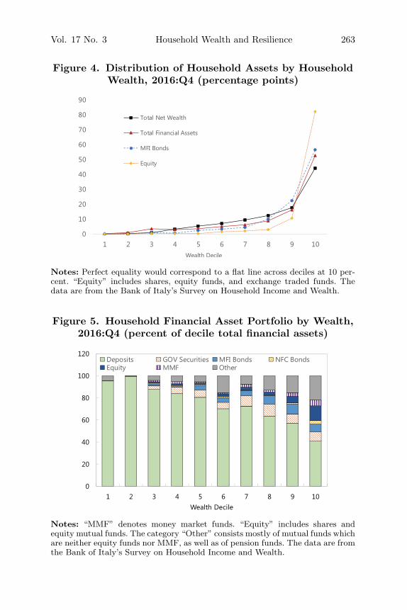
Financial wealth is concentrated at the top of the distribution(figure 4). Households at the top 20 percent of the wealth distrib-ution hold 69 percent of financial wealth. This is particularly thecase for risky assets, such as equity holdings (93 percent at the top20), and to a lesser extent for bank bonds (79 percent at the top20). Government bonds are distributed in line with total financialwealth.

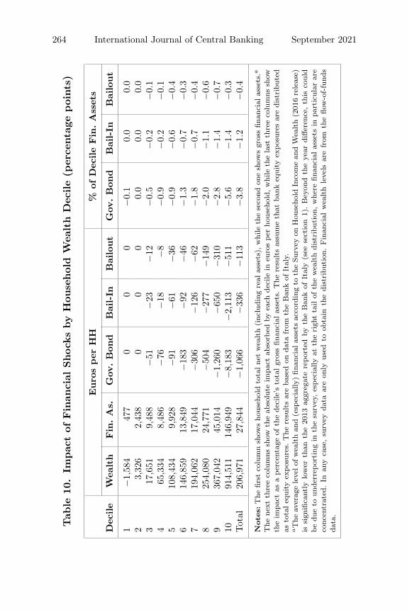
Wealthier households hold riskier financial instruments (figure 5).The financial portfolio of less-wealthy households is almost entirelyconstituted by (insured) bank deposits, so they are not directlyaffected by government bond or bank financial shocks. Wealthierhouseholds, with a higher capacity to absorb losses, invest propor-tionally more in equity and nonsecured fixed-income instruments.Yet, most of their financial wealth is also in safe assets.

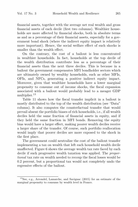
As a result, wealthy households absorb most of the financiallosses after a government bond shock or a bail-in. Table 10 shows theimpact of the three financial shocks by household decile, expressedboth in euros per household and as a percentage of decile total


Figure 4. Distribution of Household Assets by HouseholdWealth, 2016:Q4 (percentage points)

Notes: Perfect equality would correspond to a flat line across deciles at 10 per-cent. “Equity” includes shares, equity funds, and exchange traded funds. Thedata are from the Bank of Italy’s Survey on Household Income and Wealth.

Figure 5. Household Financial Asset Portfolio by Wealth,2016:Q4 (percent of decile total financial assets)

Notes: “MMF” denotes money market funds. “Equity” includes shares andequity mutual funds. The category “Other” consists mostly of mutual funds whichare neither equity funds nor MMF, as well as of pension funds. The data are fromthe Bank of Italy’s Survey on Household Income and Wealth.


Tab

le10

.Im

pac

tof

Fin

anci

alShock

sby

Hou

sehol

dW

ealth

Dec

ile

(per

centa

gepoi

nts

)

Euro

sper

HH

%of

Dec

ile

Fin

.A

sset

s

Dec

ile

Wea

lth

Fin

.A

s.G

ov.B

ond

Bai

l-In

Bai

lout

Gov

.B

ond

Bai

l-In

Bai

lout

1−

1,58

447

70

00

−0.

10.

00.

02

3,32

62,

438

00

00.

00.

00.

03

17,6

519,

488

−51

−23

−12

−0.

5−

0.2

−0.

14

65,3

348,

486

−76

−18

−8

−0.

9−

0.2

−0.

15

108,

434

9,92

8−

91−

61−

36−

0.9

−0.

6−

0.4

614

6,85

913

,849

−18

3−

92−

46−

1.3

−0.

7−

0.3

719

4,06

217

,044

−30

6−

126

−62

−1.

8−

0.7

−0.

48

254,

080

24,7

71−

504

−27

7−

149

−2.

0−

1.1

−0.

69

367,

042

45,0

14−

1,26

0−

650

−31

0−

2.8

−1.

4−

0.7

1091

4,51

114

6,94

9−

8,18

3−

2,11

3−

511

−5.

6−

1.4

−0.

3Tot

al20

6,97

127

,844

−1,

066

−33

6−

113

−3.

8−

1.2

−0.

4

Note

s:T

hefir

stco

lum

nsh

ows

hous

ehol

dto

talne

tw

ealth

(inc

ludi

ngre

alas

sets

),w

hile

the

seco

ndon

esh

ows

gros

sfin

anci

alas

sets

.a

The

next

thre

eco

lum

nssh

owth

eab

solu

teim

pact

abso

rbed

byea

chde

cile

ineu

ros

per

hous

ehol

d,w

hile

the

last

thre

eco

lum

nssh

owth

eim

pact

asa

per

cent

age

ofth

ede

cile

’sto

talgr

oss

finan

cial

asse

ts.T

here

sults

assu

me

that

bank

equi

tyex

pos

ures

are

dist

ribu

ted

asto

taleq

uity

expos

ures

.T

here

sults

are

base

don

data

from

the

Ban

kof

Ital

y.aT

heav

erag

ele

velof

wea

lth

and

(esp

ecia

lly)

finan

cial

asse

tsac

cord

ing

toth

eSu

rvey

onH

ouse

hold

Inco

me

and

Wea

lth

(201

6re

leas

e)is

sign

ifica

ntly

low

erth

anth

e20

13ag

greg

ate

repor

ted

byth

eB

ank

ofIt

aly

(see

sect

ion

1).

Bey

ond

the

year

differ

ence

,th

isco

uld

be

due

toun

derr

epor

ting

inth

esu

rvey

,es

pec

ially

atth

eri

ght

tail

ofth

ew

ealth

dist

ribu

tion

,w

here

finan

cial

asse

tsin

part

icul

arar

eco

ncen

trat

ed.

Inan

yca

se,

surv

eyda

taar

eon

lyus

edto

obta

inth

edi

stri

bution

.Fin

anci

alw

ealth

leve

lsar

efr

omth

eflo

w-o

f-fu

nds

data

.


financial assets, together with the average net real wealth and grossfinancial assets of each decile (first two columns). Wealthier house-holds are more affected by financial shocks, both in absolute termsas and as a percentage of their financial assets, especially for a gov-ernment bond shock (where the indirect equity impact is relativelymore important). Hence, the social welfare effect of such shocks issmaller than the wealth effect.

On the contrary, the cost of a bailout is less concentratedin wealthier households. In fact, households at the top decile ofthe wealth distribution contribute less as a percentage of theirfinancial assets than the next three deciles. This is because in abailout the government compensates MFI bondholder sectors whichare ultimately owned by wealthy households, such as other MFIs,OFIs, and NFCs, generating a positive indirect equity impact.Moreover, given that wealthier households have a lower marginalpropensity to consume out of income shocks, the fiscal expansionassociated with a bailout would probably lead to a meager GDPmultiplier.13

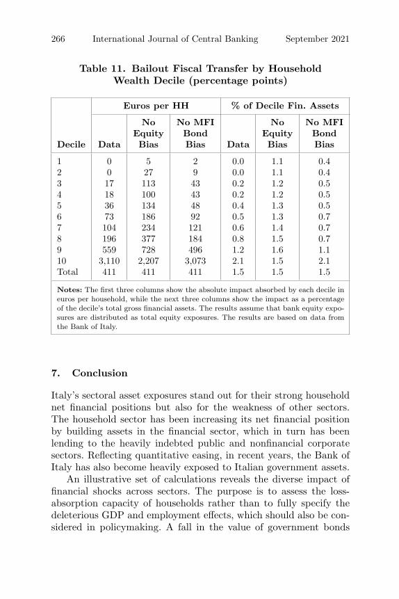
Table 11 shows how the fiscal transfer implicit in a bailout ismostly distributed to the top of the wealth distribution (see “Data”column). It also computes the counterfactual transfer that wouldprevail absent the portfolio biases of rich households, i.e., if all wealthdeciles held the same fraction of financial assets in equity, and ifthey held the same fraction in MFI bonds. Removing the equitybias would have a larger effect, making poorer wealth deciles receivea larger share of the transfer. Of course, such portfolio reallocationwould imply that poorer deciles are more exposed to the shock inthe first place.

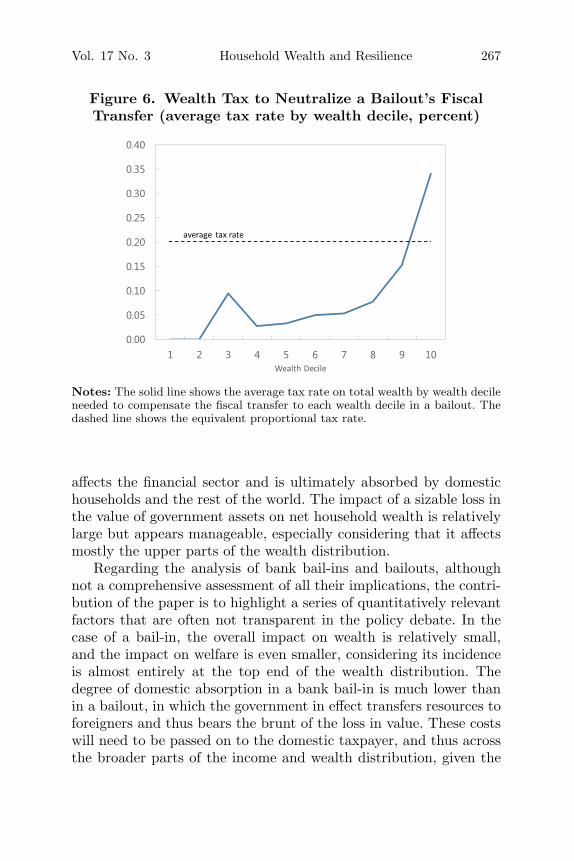
The government could neutralize the cost of the bailout transferimplementing a tax on wealth that left each household wealth decileunaffected. Figure 6 shows the average wealth tax rate faced by eachdecile if such progressive wealth taxation was applied. The propor-tional tax rate on wealth needed to recoup the fiscal losses would be0.2 percent, but a proportional tax would not completely undo theregressive effects of the bailout.

13See, e.g., Arrondel, Lamarche, and Savignac (2015) for an estimate of themarginal propensity to consume by wealth level in France.


Table 11. Bailout Fiscal Transfer by HouseholdWealth Decile (percentage points)

Euros per HH % of Decile Fin. Assets

No No MFI No No MFIEquity Bond Equity Bond

Decile Data Bias Bias Data Bias Bias

1 0 5 2 0.0 1.1 0.42 0 27 9 0.0 1.1 0.43 17 113 43 0.2 1.2 0.54 18 100 43 0.2 1.2 0.55 36 134 48 0.4 1.3 0.56 73 186 92 0.5 1.3 0.77 104 234 121 0.6 1.4 0.78 196 377 184 0.8 1.5 0.79 559 728 496 1.2 1.6 1.110 3,110 2,207 3,073 2.1 1.5 2.1Total 411 411 411 1.5 1.5 1.5

Notes: The first three columns show the absolute impact absorbed by each decile ineuros per household, while the next three columns show the impact as a percentageof the decile’s total gross financial assets. The results assume that bank equity expo-sures are distributed as total equity exposures. The results are based on data fromthe Bank of Italy.

7. Conclusion

Italy’s sectoral asset exposures stand out for their strong householdnet financial positions but also for the weakness of other sectors.The household sector has been increasing its net financial positionby building assets in the financial sector, which in turn has beenlending to the heavily indebted public and nonfinancial corporatesectors. Reflecting quantitative easing, in recent years, the Bank ofItaly has also become heavily exposed to Italian government assets.

An illustrative set of calculations reveals the diverse impact offinancial shocks across sectors. The purpose is to assess the loss-absorption capacity of households rather than to fully specify thedeleterious GDP and employment effects, which should also be con-sidered in policymaking. A fall in the value of government bonds


Figure 6. Wealth Tax to Neutralize a Bailout’s FiscalTransfer (average tax rate by wealth decile, percent)

Notes: The solid line shows the average tax rate on total wealth by wealth decileneeded to compensate the fiscal transfer to each wealth decile in a bailout. Thedashed line shows the equivalent proportional tax rate.

affects the financial sector and is ultimately absorbed by domestichouseholds and the rest of the world. The impact of a sizable loss inthe value of government assets on net household wealth is relativelylarge but appears manageable, especially considering that it affectsmostly the upper parts of the wealth distribution.

Regarding the analysis of bank bail-ins and bailouts, althoughnot a comprehensive assessment of all their implications, the contri-bution of the paper is to highlight a series of quantitatively relevantfactors that are often not transparent in the policy debate. In thecase of a bail-in, the overall impact on wealth is relatively small,and the impact on welfare is even smaller, considering its incidenceis almost entirely at the top end of the wealth distribution. Thedegree of domestic absorption in a bank bail-in is much lower thanin a bailout, in which the government in effect transfers resources toforeigners and thus bears the brunt of the loss in value. These costswill need to be passed on to the domestic taxpayer, and thus acrossthe broader parts of the income and wealth distribution, given the


heavy reliance on labor income and consumption taxes as opposedto wealth taxes.

Appendix A. Identification of SectoralLinkages in the Data

This appendix describes the necessary assumptions to infer intersec-toral exposures from Italian flow-of-funds data.

For some sector-instruments, such as government bonds, identi-fying the counterparty sector is straightforward—the government.If the counterparty sector of an instrument is reported as “otherfinancial institutions,” the assets are distributed between OFI andINP according to the relative total liabilities of these two sectors inthat particular instrument. A similar assumption applies to instru-ments issued by MFIs when the data does not specify whether theseare issued by the Bank of Italy or other MFIs (e.g., deposits). Forinstrument categories “short-term loans,” “medium- and long-termloans,” and “insurance, pension, and guaranteed funds,” the datado not provide a complete sectoral disaggregation on the asset side.Hence, the classification is based on liability-side information.

For the remaining sector-instruments, the principle of maxi-mum entropy is applied, following previous literature (most closelyCastren and Kavonius 2009, inspired by Allen and Gale 2000). Thatis, asset positions of sector i on sector j are obtained multiplying themarginal distribution of sector i assets times the marginal distrib-ution of sector j liabilities. Typically, these “unclassifiable” instru-ments are reported in the data as assets of sector i in “other sectors”or liabilities of sector i with respect to “other sectors.”

This classification approach ensures that all instruments are allo-cated to both a creditor and a debtor sector. Hence, the total sumof assets and liabilities in each instrument is consistent with thebalance sheet positions of the whole economy in that instrument.

Appendix B. Financial Exposures over Time

Table B.1 contains the full matrix of bilateral exposures at selectpoints in time: (i) the beginning of the sample, 1995:Q1; (ii) thedeployment of the euro, 2001:Q4; (iii) the onset of the GFC, 2008:Q1;


Table B.1. Sectoral Financial Asset Exposures over Time(percent of GDP)

1995:Q1 NFC MFI BOI OFI INP GOV HH RoW Tot. As. NFA

NFC 7 2 1 2 5 5 10 33 −67MFI 39 2 2 0 25 16 14 97 −1BOI 0 2 0 0 9 0 5 17 3OFI 7 3 0 0 5 1 6 21 0INP 2 2 0 0 4 0 2 9 −5GOV 9 5 1 6 1 1 2 24 −77HH 33 54 8 11 10 35 10 162 139RoW 11 24 1 1 1 18 0 56 8Tot. Liab. 100 98 14 21 14 102 23 48 418







(continued)


Table B.1. (Continued)


NFC 14 7 1 2 6 5 27 61 −112MFI 54 5 13 1 37 37 23 170 0BOI 0 16 0 0 22 0 13 53 6OFI 11 18 2 0 8 4 26 69 27INP 4 3 1 3 20 0 25 55 −2GOV 11 5 1 4 1 4 4 30 −124HH 54 64 19 16 50 14 30 247 196RoW 39 50 12 6 3 47 1 157 8Tot. Liab. 174 170 47 42 56 154 51 149 843

Notes: The data are from the Bank of Italy.

(iv) the Outright Monetary Transactions program announcement,2012:Q2; and (v) the end of the sample, 2017:Q3.

Appendix C. Bank Shock Counterfactual Simulations

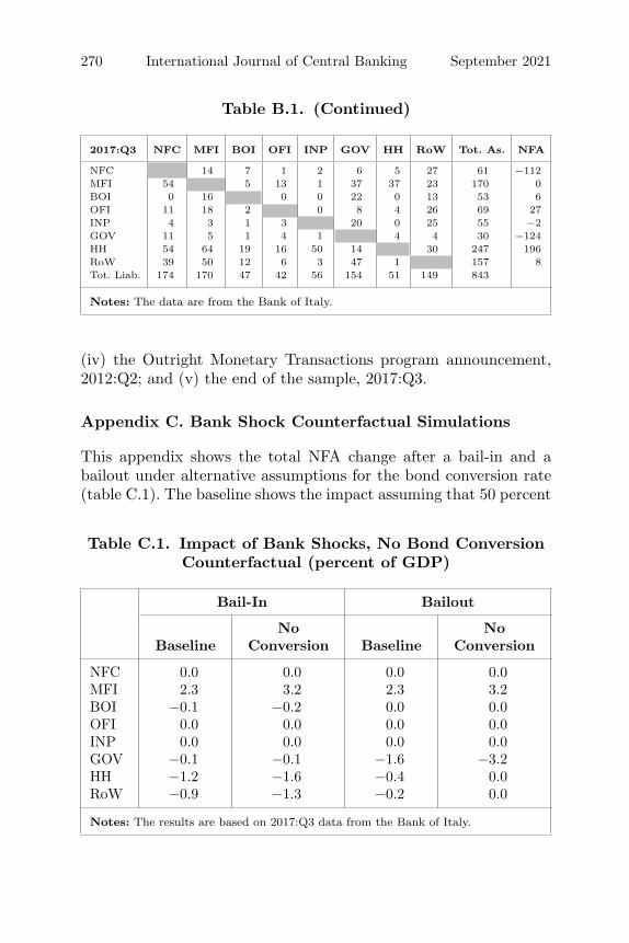
This appendix shows the total NFA change after a bail-in and abailout under alternative assumptions for the bond conversion rate(table C.1). The baseline shows the impact assuming that 50 percent

Table C.1. Impact of Bank Shocks, No Bond ConversionCounterfactual (percent of GDP)

Bail-In Bailout

No NoBaseline Conversion Baseline Conversion

NFC 0.0 0.0 0.0 0.0MFI 2.3 3.2 2.3 3.2BOI −0.1 −0.2 0.0 0.0OFI 0.0 0.0 0.0 0.0INP 0.0 0.0 0.0 0.0GOV −0.1 −0.1 −1.6 −3.2HH −1.2 −1.6 −0.4 0.0RoW −0.9 −1.3 −0.2 0.0

Notes: The results are based on 2017:Q3 data from the Bank of Italy.


of the value of bonds is recovered after bonds are converted to equity,while the alternative shows the impact under a zero conversion rate.

A lower conversion rate increases total bondholder losses andthus the required government transfer in a bailout. In the bail-incase, the additional impact is roughly proportionally distributedacross sectors.

References

Albertazzi, U., T. Ropele, G. Sene, and F. M. Signoretti. 2014. “TheImpact of the Sovereign Debt Crisis on the Activity of Ital-ian Banks.” Journal of Banking and Finance 46 (September):387–402.

Allen, F., and D. Gale. 2000. “Financial Contagion.” Journal ofPolitical Economy 108 (1): 1–33.

Arrondel, L., P. Lamarche, and F. Savignac. 2015. “Wealth Effectson Consumption Across the Wealth Distribution: Empirical Evi-dence.” ECB Working Paper No. 1817.

Bank of Italy. 2014. “Household Wealth in Italy in 2013.” No. 69,Supplements to the Statistical Bulletin.

Bofondi, M., L. Carpinelli, and E. Sette. 2018. “Credit Supply dur-ing a Sovereign Debt Crisis.” Journal of the European EconomicAssociation 16 (3): 696–729.

Castren, O., and I. K. Kavonius. 2009. “Balance Sheet Interlink-ages and Macro-financial Risk Analysis in the Euro Area.” ECBWorking Paper No. 1124.

Cingano, F., F. Manaresi, and E. Sette. 2016. “Does Credit CrunchInvestment Down? New Evidence on the Real Effects of theBank-Lending Channel.” Review of Financial Studies 29 (10):2737–73.

Cortes, F., P. Lindner, S. Malik, and M. A. Segoviano. 2018.“A Comprehensive Multi-Sector Tool for Analysis of SystemicRisk and Interconnectedness (SyRIN).” IMF Working Paper No.18/14.

Doepke, M., and M. Schneider. 2006. “Inflation and the Redistribu-tion of Nominal Wealth.” Journal of Political Economy 114 (6):1069–97.

Gourinchas, P. O., P. Martin, and T. Messer. 2017. “The Economicsof Sovereign Debt, Bailouts and the Eurozone Crisis.” Mimeo.


Heipertz, J., R. Ranciere, and N. Valla. 2017. “Domestic and Inter-national Sectoral Portfolios: Network Structure and Balance-Sheet Effects.” NBER Working Paper No. 23572.

Huser, A.-C., G. Ha�laj, C. Kok, C. Perales, and A. van der Kraaij.2018. “The Systemic Implications of Bail-in: A Multi-layeredNetwork Approach.” Journal of Financial Stability 38 (October):81–97.

International Monetary Fund. 2015. “Balance Sheet Analysis inFund Surveillance.” IMF Policy Paper (June).

Jensen, M. C., and W. H. Meckling. 1976. “Theory of the Firm:Managerial Behavior, Agency Costs and Ownership Structure.”Journal of Financial Economics 3 (4): 305–60.

Koijen, R. S. J., F. Koulischer, B. Nguyen, and M. Yogo. 2018.“Quantitative Easing in the Euro Area: The Dynamics of RiskExposures and the Impact on Asset Prices.” Working Paper No.601, Banque de France.

Lindner, P., and V. Redak. 2017. “The Resilience of Householdsin Bank Bail-ins.” In Financial Stability Report No. 33, 88–101. Vienna: Oesterreichische Nationalbank (Austrian NationalBank).

Poterba, J. M. 1987. “Tax Policy and Corporate Saving.” BrookingsPapers on Economic Activity 2: 455–515.

household wealth and resilience to financial shocks in italy

Documents