Housing Prices and Land Use Regulations: A Study of 250 Major US Cities♣♦

© Theo S. Eicher

University of Washington Income and population growth are key determinants of housing demand, while land use regulations are designed to affect housing supply. Previous studies of housing price determinants focus either on specific regulations in particular cities/regions, or on selective subsets of major cities and regulations. This study examines the impact of land use regulations on housing prices in 250 major US cities from 1989 to 2006. Aside from factors that are commonly associated with housing demand (income, population growth and density), housing prices are found to be associated with local cost-increasing land use regulations (approval delays) and with statewide regulations. Since statewide regulations factor prominently into the results, specific examples of the impact of different types of land use regulations are provided for 5 cities in the state of Washington. The estimated increase in housing prices associated with regulations is, on average (over 250 cities), substantially larger than the effects of income and population growth. While the estimated dollar costs associated with regulations may be sizable at times, the results are remarkably consistent with previous studies that were based on smaller cross sections.

♣Draft 5/2/08. Do not cite or distribute without permission, te@u.washington.edu. ♦I thank Kriss Sjoblom, Dick Conway, Debora I. Dusselich, Kenneth J. Dueker, Hart Hodges, Richard Allen Nelson, Lillian Lyons, Marty Lyons, Catherine O'Donnell, and Bob Roseth for helpful comments.

1

1. Introduction

Housing prices follow the fundamental laws of supply and demand. The challenge for

economists is to identify the specific factors that are associated with housing supply and demand.

Economic theory is clear: changes in housing prices are associated primarily with income and

demographic factors on the demand side, and with costs considerations (e.g., land use

regulations) on the supply side.1 Price, income, and demographic data are readily available from

government sources, but it has proven to be extraordinarily costly and time consuming to obtain

objective and comparative land use regulation data for informative, representative studies.

In surveying the housing literature, one is struck by the abundance of studies that focus

on the effects of specific regulations in particular cities. Authors surveying the literature at times

succumb to the temptation of generalizing results from the numerous city/region-specific studies,

in hopes of establishing broad patterns that link regulations to housing prices (see, for example

Nelson et al. 2004).2 Although studies of individual jurisdictions may be informative, it is

unclear whether it is possible to generalize their findings. For example, the economic impact of

zoning restrictions that affect lot sizes in California are distinctly different from building height

restrictions in New York. Individual city studies may also be susceptible to “selection bias” by

which researchers’ site selection and data collection may systematically influence results to

validate prior expectations. Even cross-city studies that examine several dozen major

metropolitan areas may be subject to selection bias. Glaeser and Gyourko (2002) point out, for

example, that smaller datasets which feature only large metropolitan areas may oversample

highly regulated cities and underrepresent the bulk of American housing that featured robust

growth and available land.

This paper examines 250 major US cities documents to identify the effects of land use

regulations on housing prices. This regulatory dataset was produced by an extensive land use

study at the Wharton Business School for the University of Pennsylvania. Researchers at

Wharton’s Zell/Lurie Real Estate Center executed a nationwide survey of residential land use 1 At times public opinion and policy makers seem to be taken aback that housing prices depend on regulations. It is the expressed purpose and design of regulations to influence the housing supply. The conceptual framework in Section 3 clarifies that housing prices may rise or fall due to regulations. 2 Nelson et al. (2004) are often cited as providing academic evidence that regulations do not affect housing prices. Even cursory reading of the executive summary reveals that such statements are at odds with the conclusions of their paper. The authors present only their perspectives on previous housing studies, not original work. Connerly (2004) summarizes the evidence surveyed in Nelson et al. (2004); Appendix 3 Table A3.2 reproduces Connelly’s Table.

2

regulations in over 2,700 US communities (Gyourko et al., 2008). Aside from legal variables, the

Wharton database is therefore not based on researchers’ or consultants’ assessments but it

represents data collected from each city’s planning director that is now made available to

researchers. The dataset provides a first opportunity to examine the specific regulations that can

be associated with changes in housing prices across a large number of US cities. The broad cross

section approach eliminates nagging doubts whether a particular result for a particular city is also

relevant to other regions.

Often-cited reasons for the escalation of US housing prices in the past 10-20 years

include lower mortgage rates, creative mortgages, and income/employment growth. These

factors, which may well contribute to increasing housing prices, all relate exclusively to housing

demand. Housing supply factors, however, are harder to quantify and are typified by opposing

view points: for example, environment vs. sprawl, builders vs. planners, parks vs. high-rises, and

state vs. local growth management. Growth management often refers to: 1) urban growth

boundaries, 2) regulation of development densities (e.g., minimum lot-size rules), and 3) cost-

increasing regulations (facility development and/or regulatory delays in the approval process).

The Wharton database provides objective and comparative information on 70 land use

regulations that cover growth boundaries, density and cost-increasing regulations. This paper

reports how this data can be used in regression analysis3 to identify the effects of land use

regulations on housing prices. The results are highly statistically significant4 and indicate a

substantial association between regulations and changes in housing prices. Aside from demand

factors, four regulations are shown to be robustly related to changes in real housing prices across

the 250 cities between 1989 and 2006: 1) permit delays, 2) statewide land use regulations, 3)

court support for statewide regulations, and 4) growth management.

Since these regulations speak to both local and state wide regulations, it is useful to

provide an example of the effects of regulations on different cities within one state. Such an

3 For non-economists, footnotes are included below to provide brief background information for key statistical terms throughout the paper. ”Regression analysis” is a statistical method used to examine relationships between a variable of interest (housing prices in this case) and explanatory variables. Regressions allow the researcher to estimate the quantitative effect of explanatory variables upon the variable of interest. The reported “statistical significance” of regressors then indicates a degree of confidence that the true relationship is close to the estimated effect. 4 “Statistical significance” is an expression in statistics that indicates how likely it is that an event occurred by pure chance. So a 99 percent significance level indicates that there is a 1 percent chance that the finding could be the result of a random accident.

3

example can highlight that the costs of regulations can differ even within a particular state

(Washington State) among cities that are subject to similar statewide regulations. The variations

in the costs of regulation are then due to substantially different local regulation and demand

environments, as well as the degrees to which municipalities are affected by the statewide

regulations. While the magnitudes reported may seem surprisingly large, Section 6.1 shows that

these findings are remarkably consistent with results from a number of previous studies based on

smaller cross sections of cities.

Combining the 2730 cities in the Wharton Sample with 2006 Census data renders a

sample of 250 major US cities. The city of Seattle features prominently among these cities: it

ranks 5th among all cities in terms of overall land use restrictions as measured by the Wharton

Residential Land Use Regulatory Index, and also 5th in terms of permit and zoning approval

delays. Seattle also belongs to the group of cities that ranks first among all cities in terms of the

impact of state political involvement and growth management.5 Across all 2730 cities in the

sample, Appendix 2 shows that many of Washington’s cities rank in the top 10 percent in terms

of land use restrictions across a variety of regulatory measures.6 This warrants a discussion of

Seattle in specific, and Washington State in general. The comparison highlights that the city-

specific impacts of statewide land use regulations may vary substantially across municipalities.

The focus on the link between regulatory restrictions and housing prices is controversial

in the planning literature. As Glaeser (2004) points out, housing demand factors have long been

considered central determinants of housing prices. In the early 1980s, Poterba (1984) and

Summers (1981) documented that inflation increased the interest rate subsidy on mortgages to

such an extent that the resulting shift in housing demand explained much of the run up in

housing prices in the 1970s. Mankiw and Weil (1991) highlighted that demographics also drive

housing demand. Given the aging of the US population, their results yielded the ominous

prediction that “real housing prices will fall substantially over the next two decades.” Contrary to

5 Seattle ranks in the top 10% for State Court Involvement in Regulations, State Legislature Involvement in Regulations, Total # of Initiatives 1996-2005, Local Political Pressure Index, Environmental Review Board Requirements, Permit Lag for Subdivisions Approval (<50 units), Community Pressure Involvement in Regulations, Permit Lag for Subdivisions Approval (multi family project), Permit Lag for Rezoning (<50 units), Permit Lag for Rezoning (multi family project), Permit Lag for Review Time (multi family project), Permit Lag for Review Time (single family), Permit Lag for Rezoning, (>50 units), Design Review Board Approval Requirements. 6 About 50 other Washington cities were included in the Wharton sample; see Appendix 2.

4

the Mankiw and Weil forecast, housing prices across 250 major US cities rose 54 percent (after

accounting for inflation) from 1989-2006.7

Housing supply determinants have only recently come under intense scrutiny. Seminal

was the special issue of the Journal of Real Estate Finance and Economics devoted to housing

supply (Rosenthal, 1999), which contains several surveys that cover distinct dimensions of

housing supply. Subsequently, Green et al. (2005) estimate a detailed housing supply function

for 45 major cities. This line of research has culminated in a voluminous literature that

documents a robust association between housing prices and the stringency of land use

regulations. Glaeser (2004) summarizes the evidence and provides broad and compelling support

from studies of US regions and cities (see also Appendix 3).

Finally, it is also important to highlight that the economic analysis below provides cost

estimates of regulations, but it cannot identify whether such regulations are socially optimal. For

the same reason it cannot provide value judgments that identify regulations as “good,” “bad,” or

“misguided.” Think about it this way: citizens may well value regulations even more than the

price they have to pay for them! Nelson et al. (2004) make this point forcefully when they point

out that growth restrictions in Boulder, Colorado, drove up the price of housing near green belts,

and that this price increase reflected nothing other than the willingness to pay (in the sense that

wealthier citizens simply revealed their preference for pretty views).

What is often neglected, however, is that these very examples also highlight that

regulations and affordable housing have been mutually exclusive (see, e.g., Seattle Times, 2008).

In the absence of normative guidance, it falls to the electorate to decide whether the benefits

derived exceed the associated costs in terms of housing price increases. Alternatively, the cost

estimates here provide guidance that can assist policy reviews/updates. As Nelson et al. (2004)

point out, “if housing prices may increase in any land use environment, then the decision is

between good and bad regulation to improve housing choice.” Brueckner (2007) reminds us that

growth management policy interventions “are often well-meaning, being designed to achieve

ends that are thought to be socially desirable.” The problem is that the complexity of the urban

real estate markets may create subsidiary effects that are either unanticipated or unforeseen by

policy makers and planners alike. To assure against adverse effects, policy review must be

frequent to reoptimize when unintended effects compromise the designed effects of regulations.

7 Based on Census data for median real price of owner-occupied housing described in detail below.

5

2. Previous Comparative Studies of Housing Prices and Regulations

2.1 Comparative Studies of US Metropolitan Areas

A large number of studies exist that examine the effects of specific demand and supply

factors on housing prices in particular cities. As discussed in the introduction, it is difficult to

derive general implications from such studies. Instead, the results below are based on a large

cross section. Before these results are presented, however, it is important to review the methods

and findings from previous cross sectional studies of housing prices and regulations. This

review focuses only on relationships between housing prices and regulations. Other papers, not

cited below, focus on the impact of regulations on permits, construction, and land availability.

Black and Hoben (1985) first developed a measure of “restrictive”, “normal”, or

“permissive” regulations for 30 US metropolitan areas. They report a correlation of –0.7 between

their regulation index and 1980 prices for developable lots.8 Segal and Srinivasan (1985)

surveyed planning officials in 51 metropolitan areas to find the percentage of undeveloped land

taken out of production due to land use regulations. They estimated that regulated cities have 1.7

percent faster annual housing price increases than unregulated cities. With compounding, this

actually turns out to generate a dramatic impact on housing prices over a decade (about 20

percent). As an alternative, Guidry et al. (1991) employed land use and environmental data from

the American Institute of Planners (AIP, 1976) to find that land prices in cities with more

stringent land use controls increased 16 percent for every 10 percent increase in their regulatory

measure. Guidry et al. (1991) also examined regulation data from the Urban Land Institute9 to

find that average lot prices in the most restrictive cities in 1990 were about $26,000 higher, than

in the least regulated cities.

One of the most prominent comparative studies is Malpezzi (1996) who examines 56 US

metropolitan areas. He built his analysis on regulatory data collected by the Wharton Urban

Decentralization Project carried out by Linneman et al. (1990).10 Despite its comparatively large

8 To obtain a visual example how tight a -0.7 correlation is, see http://en.wikipedia.org/wiki/Correlation. 9 The data is based on a survey of 11 real estate experts who ranked land use restrictiveness of 30 metropolitan areas on a 10-point scale. Instead of a single regulation criterion, the survey covered 6 broad areas of land use regulations. The Urban Land Institute data covers: 1) wet land management, 2) power plant regulation, 3) critical areas and wilderness, 4) strip mining, 5) flood plains, and 6) tax incentives. The variable is unfortunately binary, indicating only whether regulations exist or not. 10 Unfortunately, communication with the authors of the study indicates that this data has been lost.

6

coverage, Malpezzi’s data lacks information on key metropolitan areas (such as Seattle). He

focuses squarely on cost-increasing regulations (zoning and permit time costs) and adds a

variable to indicate when states regulate environmental impacts (coastal, wetland or floodplain

management). His findings imply that moving from lightly regulated to highly regulated cities

reduces housing permits by 42 percent and increases housing prices by 51 percent. Malpezzi et

al. (1998) use a hedonic price index and show that regulations increased housing prices by 31-46

percent. Phillips and Goodstein examined 37 metropolitan areas and found that the Malpezzi

(1996) regulatory index was associated with higher housing prices, although a proxy for the

effect of the urban growth boundary in Portland was shown to be less than $10,000 per unit.

Downs (2002) increased the sample of metropolitan areas to 86 and examines the period of 1990

to 2000. He does not find an effect of regulations on housing prices for all periods, only for

1990-2000, 1990-94 and 1990-96.

Glaeser and Gyourko (2002) examine lot prices in 40 US cities, controlling for the

change in the cost of construction. They label the gap between the actual housing prices and the

cost of construction (minus the lot price) provocatively the “zoning tax.” Table 1 is a

reproduction of their results showing the change in housing prices relative to construction costs

in major cities and suburbs. They associate their zoning taxes with cost-increasing regulations

(time to permit issuance for zoning requests) and find a statistically significant relationship.

2.2 Comparative Regional Studies

Other large scale studies are regional, such as Katz and Rosen's (1987), who analyzed 85

cities in the San Francisco Bay area to find that housing prices increased between 17-38 percent

in communities with growth control measures. Levine (1999) expanded Katz and Rosen’s

approach to 490 Californian cities and 18 different land use measures. He finds that land use

restrictions “displaced new construction, particularly rental housing, possibly exacerbating the

expansion of the metropolitan areas into the interiors of the state.” Pollakowski and Wachter

(1990) examined 17 zoning jurisdictions in Montgomery County, Maryland, over a period of

eight years and found that a 10 percent increase in these zoning restrictions increased housing

prices by 27 percent. Interestingly, they also provided evidence on the externalities11 associated

11 An externality is an economics term that describes that a decision imposes costs or benefits to third party. This implies that agents in private economic transactions do not all bear costs or reap all benefits of the transaction.

7

with regulations: housing prices are shown to rise when the restrictiveness of zoning measures in

adjacent jurisdictions increased.

Downs (1992) examined the effects of growth management plans in San Diego County,

CA, to find a housing shortage in the five largest cities was aggravated by growth controls that

increased prices of existing homes by 54 percent and prices of new homes by 61 percent in three

years. Cho and Linneman (1993) examine 10 districts in Virginia and found that zoning

restrictions had a significant impact on housing price within the district and via spillovers to

nearby jurisdictions. Green (1999) examined zoning and permitting regulations in 39

municipalities in Wisconsin and found that two of the regulatory variables had modest impacts

on price increases. Finally, Gyourko and Summers (2006) analyze 218 jurisdictions around

Philadelphia and find that areas with average land use regulations saw slightly negative increases

in the real cost of single family lots over 10 years. The most restrictive municipalities, in

contrast, saw lot cost increases of up to 70 percent (for a summary see Appendix 3). Finally

Glaeser et al. (2006a, b) report on a study of 187 communities in eastern Massachusetts to find

that regulation, not density, has caused low levels of new construction and high housing prices in

the Greater Boston area. The reduction in permits caused by the regulations has had a significant

effect on regional housing prices, which were increased median housing prices by 23-36 percent

or about $156,000.

The sample of cities featured in this paper is roughly identical in size to the samples in

Gyourko and Sommers (2006), and Glaeser et al. (2006a, b); instead of covering only one

region, however, the sample below is comprised of 250 major US cities. It shares with previous

comparative studies that zoning restrictions and approval delays are considered, but it also

extends the focus of previous analyses to include statewide measures, such as growth

management plans and even court rulings regarding regulatory enforcement. Malpezzi (1996)

also considers statewide measures, but the structure of his data assumes that the effect of such

regulations is identical across cities. Instead, the Wharton database provides information on the

degree to which each city is impacted by statewide regulations. Finally, instead of focusing on

only one or a couple of regulations, it is also examined whether a given individual regulation in

the Wharton database potentially affects housing prices.

3. Supply and Demand for Housing

8

Before moving to the formal statistical analysis, it is important to review the basic mechanics of

housing supply and demand. The following section closely follows the lucid framework laid out

by Malpezzi (1996); it can also be found in any introductory urban/real estate economics

textbook (e.g., O’Sullivan, 2003). Figure 1 represents a simple housing market for identical

units. In a free market, supply and demand curves (S1 and D1, respectively) intersect at the

equilibrium point, A. Point A maximizes private welfare as it equates the private costs to the

private benefits for housing units.

In the presence of an externality12, however, society faces a potential market failure. In

the context of real estate economics, an example of such an externality would be the public’s

desire for parks and green spaces. Such desires raise the social cost of supplying housing above

the private cost to shift the supply curve up to S2. From society’s perspective, the equilibrium at

point A now represents “too much” housing at “too low” a price and policies that regulate

housing to coincide with point B would deliver the socially preferred outcome. The difference

between the housing quantities and prices at A and B is then the social cost of attaining the public

benefit of reduced housing. This cost includes a welfare loss that each citizen incurs due to the

reduction in housing units and the associated increase in prices.

Note that there also exist housing externalities that increase social benefits beyond

private benefits. Such externalities lower the social cost of housing supply.13 In this case, the

12 Malpezzi (1996) mentions the following externalities that raise the social cost of housing: “1. Congestion. Building additional housing units in a community generally increases traffic locally (although it may reduce total commuting distance). 2. Environmental costs. Building additional housing units may reduce the local supply of green space; reduce air quality; and increase pressure on local water, sanitation, and solid waste collection systems (although again the global impact is less clear). 3. Infrastructure costs. Costs may rise as communities invest to grapple with environmental problems and congestion. Effects will depend on whether the particular community has yet exhausted economies of scale in the provision of each type of infrastructure. 4. Fiscal effects. In addition to the obvious effects from the above, demand may increase for local public services (education, fire and police protection, new residents believing libraries should be open on Sundays in contradiction to local custom). New residents may or may not pay sufficient additional taxes to cover the marginal costs. 5. Neighborhood composition effects. New households may be different from existing households. If existing households prefer living with people of similar incomes, or the same race, they will perceive costs if people different from them move in.” 13 Malpezzi (1996) points to “1. Productivity and employment. A well-functioning housing market is generally required for a well-functioning labor market. In particular, labor mobility may be adversely affected and wages may rise to uncompetitive levels if housing markets are not elastic. 2. Health benefits. At least at some level, less crowding and improved sanitation may be associated with lower rates of mortality and morbidity. 3. Racial and economic integration. One person’s external cost may be another person’s external benefit if some households value heterogeneity, for themselves or for others. For those particularly concerned about employment of low-income households or minorities, concerns about the productivity and employment effects mentioned earlier are reinforced. 4. Externalities associated with homeownership. More housing units or lower housing prices may be associated with

9

welfare maximizing policy interventions are regulations that expand housing and lower its price

(take, for example, affordable housing requirements). The housing framework therefore

highlights two important insights: 1) there is no reason to expect housing prices to rise, due to

regulations that are intended to attain the social optimum, 2) a rise in housing prices due to

regulations indicates that policy-makers associate a negative externality with the supply of

housing. Finally, note that the cost increases associated with regulations must match the

associated social valuation. To understand whether cost increases and social valuations match

requires a clear understanding of the cost and benefits of regulations. It is easier to support

regulations when the associated costs are not identified.

The supply and demand relationships are approximated by a model that provides the

foundation to the empirical approach outlined in Section 4. Readers less interested in the exact

mechanics of the model can skip to Section 4.3. The interim sections employ economics and

statistics jargon to provide the necessary methodological foundations. The housing model

presented below is largely identical to Malpezzi (1996). More complex models of housing prices

can certainly be constructed; their empirical implementation is, however, often associated with

insurmountable obstacles.14 The below analysis is therefore a compromise that acknowledges the

tradeoff between model complexity and data availability.

The standard model of the median owner-occupied house depends on the demand and

supply of owner occupied housing, DhoQ and S

hoQ , respectively. Demand is a function of the

relative price of the median owner occupied home, hoP , median income, hoI , and demographic

variables, D , that relate to density and population size. The demand relationship can then be

formally represented as

[ ]DIPFQ hohoDD

ho ,,= . (1)

greater opportunity for homeownership. Homeownership has been argued to be associated with many desirable social outcomes, ranging from improved maintenance of the housing stock to greater political stability.” 14 Pogodzinski and Sass (1991) provide a structured review of diverse approaches to modeling the effect of housing supply on housing prices. They highlight the multitude of different regulation criteria that have been employed in regional studies, which emphasizes how tenuous the generalizations are that link “regulations” to housing prices, based on individual city studies. Green et al. (2005) provide the most sophisticated empirical implementation of a theory based housing supply model. Although they control for regulations, it is not the objective of their paper to quantify the effects of regulations on housing prices.

10

The supply of the median owner occupied housing, ShoQ , is assumed to depend on the

relative price of the median owner occupied home, hoP , land use regulations, R , and the prices

of all i inputs, SiP (e.g., construction costs)

[ ]Siho

SSho PRPFQ ,,= . (2)

Construction costs are largely set at the national level and are also considered in the

methodology as described below. Aside from construction costs, other input prices (such as land)

may themselves be contaminated by regulations. In this case, Malpezzi suggests to rewrite (2) by

substituting for SiP to represent the supply side equation as the following reduced form

[ ]RPFQ hoSS

ho ,= . (2’)

The reduced form in equation (2’) has received additional validity from Green et al. (2005), who

estimate detailed, theory-based housing supply equations and find that regulations and low

supply elasticities are strongly positively correlated with heavily regulations in metropolitan

areas. The specification in (2’) highlights that regulatory changes affect housing prices both

directly and indirectly. The direct effect of regulations is a reduction in the supply of housing and

an increase in the price of housing. An indirect effect of regulations is a change in input prices,

which would then affect the supply of housing. The statistical analysis below captures the net

impact of both the direct and indirect effects.

In equilibrium, supply and demand are equalized, allowing us to solve equations (1) and

(2’) simultaneously for the housing price. This renders housing prices a function of land use

regulations, income, and demographic variables

[ ]ε,,, DIRFP hoho = . (3)

To translate the structural model into a statistical regression model, a stochastic term, ε , is added

in (3). Evidence for omitted variables or measurement error is captured in the error term. To

examine the validity of the proposed empirical model, the properties of this error term are

examined extensively in the robustness analysis reported in Appendix 1.

4. Econometric Implementation of the Housing Model

4.1 The Empirical Model

11

The reduced form in (3) is commonly estimated “in levels,” which indicates that the

variable of interest, hoP , is the price level. In terms of the econometrics, the standard cross-

section estimator (be it ordinary least squares, or any variant that allows for non-spherical

disturbances) is only consistent when individual city characteristics (so called “fixed effects”)

can be assumed to be uncorrelated with the variable of interest. It is doubtful whether this

assumption is valid in the context of housing prices. City fixed effects, such as the designation as

state capital, proximity to Disney World, or to nature, may well drive the level of housing prices.

One approach to address fixed effects is to estimate (3) in terms of growth rates, so that the

omitted variable bias associated with city-specific fixed effects is mitigated. While “nature” and

“geographical characteristics” may influence cities’ price levels, it is a much taller order to link

them to changes in prices.

The second issue is that level regressions are generally thought to be susceptible to

spurious correlations in the absence of true causal relationships. Causality is certainly not

guaranteed in growth regressions, they do mitigate spurious correlation. This renders growth

regressions a much more stringent empirical test. Third, in contrast to level regressions, growth

regressions can address the frequent confusion in the public debate about the short and long term

drivers of housing. The demand for housing – as seen above – is determined by variables that can

change quite quickly over time (income, migration, and density). Housing supply instead is by its

very nature much more inelastic, especially in the short run (it takes months to purchase land,

obtain permits, construct a home, and sell it). Examining the change in housing prices over long

time periods (17 years, in the sample below) allows the regressions to capture the effects of both

supply and demand measures with some confidence.15

Most importantly, however, growth regressions speak effectively to the question at hand:

which variables can be associated with the change in housing prices across major US cities? Or:

did housing prices increase because of land use restrictions and/or income/population growth?

Level regressions, instead, speak only to the question of whether housing prices are high in cities

with high incomes, large populations, and extensive regulations. The estimates below are

therefore based on growth regressions where the variable of interest is the annual compounded

growth rate of housing prices from 1989-2006. This renders the regression to be estimated

15 For a complete discussion of growth vs. level regressions, see Caselli et al. (1996).

12

εββββα +++++= DensityPopIRP hoho 4

^

321ˆˆ (4)

where variables with “^” subscripts represent growth rates, Pop is the population and Density is

the population density of a particular city (see Appendix 2).16 The constant, α , is included to

account for effects that are common to all cities over this period of time. Such effects might

represent changes in the national level of unemployment, changes in mortgage rates or lending

procedures, or liquidity in the mortgage market.17

4.1 Housing Price Data

Much of the housing literature wrestles not only with the development of meaningful land use

regulation data; even the measurement of its key variable, housing prices, is subject to

controversy. There are three alternative approaches to housing prices: i) median housing prices

for owner occupied homes as reported by the Census, ii) sales price data collected by the

National Association of Realtors, and iii) so-called “hedonic” price indices that take into account

the characteristics of the housing unit. All three measures are used in the literature as each

measure features distinctly different advantages.

It has been suggested that the correlation among these three housing price measures is so

high that one should not expect the choice of the type of price data to drive qualitative results

(Malpezzi, 1996). Prices given by i) and ii) suffer the drawback that they do not control for

quality increases (such as larger homes, smaller lots, nicer appliances, etc.). While Census data

has the broadest coverage, it reports only median owner occupied housing prices. The National

Association of Realtor data features a broader breadth of data, since it is based on multiple

listings. However, multiple listing data does not capture the entire market, so ii) also does not

constitute a representative sample.

In theory, hedonic price indices adjust housing prices for housing quality. This method

requires the use of a “hedonic regression” to obtain the estimates of the contribution of each

16 Since a reduced form is estimated, coefficients are not exact supply and demand elasticities (in the sense that it is impossible to isolate exact supply and demand effects of, for example, a change in income). The coefficients do provide an estimate of the impact on prices due to changes in the right-hand-side variables. When the terms “demand” and “supply” are used below, they thus refer to variables that are associated primarily with demand and supply effects. 17 At times the relationship between prices and regulations is seen to be nonlinear (e.g., Malpezzi, 1996). This possible specification is discussed in the robustness section below.

13

housing characteristic (e.g., an extra bathroom) to the price of a home. These estimates are then

used to artificially construct an imputed quality-adjusted housing price. This quality-adjusted

price construct is as reliable and error prone as the hedonic regression itself. If the true regression

model is not known, the estimated housing price is subject to measurement and omitted variable

errors that bias the contributions of all characteristics to the imputed, quality-adjusted price.

Housing price studies seldom report the actual hedonic regressions that are the basis for the

quality-adjusted housing prices used; if the information is provided, it highlights at times the

problematic nature of the procedure.

For example, in a study of housing prices in eight Washington State counties, Crellin et

al. (2006) account for quality by controlling for a) assessed value, b) lot size, c) dwelling size,

and d) number of bathrooms. Their hedonic regressions imply that the number of bathrooms

either has no influence on housing prices or a counterintuitive effect (e.g., more bathrooms imply

lower housing prices) for some counties. Malpezzi et al. (1998) also report their hedonic

regressions, using a much larger sample than Crellin et al. (2006) by examining 373 US locations

with a median sample size of 3000 home owners each (some samples exceed 70,000 owners).

Their hedonic regressions control for 19 different housing quality characteristics; but at least one

quarter of their mean regression coefficients exhibit counterintuitive effects, and many are

estimated with such large standard errors that few characteristics can be expected to be

statistically significant (e.g., to affect the housing price). Problematic properties of hedonic

regressions then contaminate the imputed quality adjusted housing price. Heravi and Silver

(2002) have also questioned the usefulness of the hedonic approach on theoretical grounds, by

highlighting how sensitive such regressions are to the small changes in methodologies.18

The 2006 Census data does not provide sufficient information to attempt hedonic

regressions, which simplifies the choice of housing data. To cover the largest possible sample

and to avoid oversampling highly regulated cities, the only option is to follow the examples in

scholarly journals set by Malpezzi (1996), Thorson (1996), Malpezzi et al. (1998), Green (1999),

Phillips and Goldstein (2000), and Malpezzi (2002) to employ housing price data from the US

Census Bureau. Two additional sources of pricing data are at times mentioned in the public press 18 The insight that different variants of hedonic regression techniques generate fundamentally different answers dates back to at least Triplett and McDonald (1977; 150, see Diewert 2003). In markets with finite numbers of goods, Pakes (2003) details the various biases of the hedonic regressions and outlines necessary conditions when proper hedonic indices can be constructed.

14

(though never in large cross sectional studies). One is the Standard & Poor's/Case-Shiller Home

Price Index, the other is the Shelter Component of the Consumer Price Index (CPI) produced by

the US Bureau of Labor Statistics.

The S&P/Case-Shiller data controls best for housing quality as it tracks repeat sales of

specific single family homes. Going back to 1990, the index features, however, only 15

metropolitan areas and excludes new construction. The exclusion of new construction is

especially relevant to the analysis here, since new construction represents the balance between

housing supply and demand in unrestricted markets. The cost of not using the quality adjusted

S&P index turns out to be small. The index produces similar growth rates of housing prices as

the US Census data used below. For example, for Seattle, LA, NY, San Francisco, Denver,

Boston, Portland and San Diego, the difference between the nominal annual growth (1989/90-

2006) in housing prices for the Standard & Poor's/Case-Shiller metropolitan areas and the

Census cities is less than 1 percent.19

The Shelter Component of the CPI is both controversial and problematic. It experienced

nine major revisions since its inception in 1950 and two fundamental revisions over the period of

analysis in this paper. The Shelter Component tracks only consumption-related housing costs

while regulations affect the asset price of a home. Housing consumption costs are essentially

proxied by the apartment rental prices and an implicit “rental equivalence” that had been imputed

for owner occupied housing. Since the Bureau of Labor Statistics’ 1997 revision of the shelter

component, it is widely acknowledged that the measure has “lost what little connection it had

recognized between the rental and owner-occupied markets” (Carson, 2006). This disconnect is

reflected in the sharp rise in housing prices in the early 2000s (as tracked by the Bureau of Labor

Statistics’ own data), which was associated with a sharp drop in home owners’ “rental

equivalence” (perhaps due to the lower cost of funds or factors specific to the rental market).

4.2 Housing Demand Data

Census data for the 2730 jurisdictions in the Wharton database are available only from

the decennial Census. To provide a timely analysis, the 2006 Census Bureau’s Public-Use

19 The unit of analysis is the “city” for the Census and the “metropolitan area” for S&P data. Therefore the data is not directly comparable (for example, Detroit City experienced a 4 percent greater nominal annual growth in housing prices than the Detroit metropolitan area). Nevertheless it is important to report that the quality adjusted S&P data features an even greater correlation with the Wharton Index than the Census data.

15

Microdata Sample (PUMS) is used here, which covers a sample of major US cities with a

minimum of 10,000 inhabitants. The intersection between the 2730 jurisdictions in the Wharton

Database and the 2006 PUMS Census data renders a universe of about 250 cities (depending on

the exact variable). The Census is also the source of the population data that was used to

calculate population and land area (to obtain city density). Finally, the Census also provided data

on median household income. Summary statistics are provided in Appendix 2.

4.3 Land Use Regulation Data

As mentioned in the introduction, the land use literature is now fortunate enough to find

at its disposal a full dataset of 70 land use indicators. The Wharton Regulatory Database speaks

to all three major components of land use regulations: urban growth boundaries, regulation of

development densities, and cost-increasing regulations. A list of the data collected in the

Wharton database is provided in Table 2. Many of these variables are highly correlated; therefore

Gyourko et al. (2008) suggest the construction of a “Wharton Index” (formally the Wharton

Residential Land Use Regulation Index).

The Wharton Index itself is composed of 11 sub-indices that reflect i) Local Political

Pressure, ii) State Political Involvement Index, iii) State Court Involvement Index, iv) Local

Zoning Approval Index, v) Local Project Approval Index, vi) Local Assembly Index, vii) Density

Restrictions Index, viii) Open Space Index, ix) Exactions Index, x) Supply Restrictions Index, and

xi) Approval Delay Index. The exact definitions of these indices are documented in Gyourko et

al. (2008). One key sub-index is the Approval Delay Index, which will be of consequence below.

It is defined as the average time lag (in months) for three types of projects: i) relatively small,

single-family projects involving fewer than 50 units; ii) larger single-family developments with

more than 50 units, and iii) multifamily projects of indeterminate size. Table 3 ranks the 50 states

by their regulatory stringency (Washington State is the 7th most regulated state) and Table 4

provides the rankings for metropolitan areas (the Seattle metropolitan is ranked 5th most

regulated in the nation).

Gyourko et al. (2008) report average regulatory statistics by state and by metropolitan

area. While it is common to use major metropolitan areas as the unit of analysis in cross sectional

studies, actual city limits are used in the regressions below, since some important metropolitan

areas are missing data for crucial cities that constitute substantial segments of the metropolitan

16

region (for example, the Seattle metropolitan is lacking information on Bellevue). Most

importantly, however, the land use data was collected at the city level; hence a city-level analysis

best reflects the relationship between the observed prices and regulations. While the Wharton

Index is informative as a broad measure of regulations, it is also of interest to conduct a deeper

analysis that identifies which of the Wharton Index’ subcomponents may be related to changes in

housing price. Examining each specific subcomponent’s explanatory power results in a clearly

defined and readily interpretable set of variables associated with changes in housing prices.

5. Estimates of Supply and Demand Effects on Housing Prices

Figures 2a-d report simple correlations between the annual compounded growth in

housing prices and the Wharton Index (Figure 2a), income growth (Figure 2b), population

growth (Figure 2c), and population density (Figure 4d). The Figures exhibit clear, positive

correlations, but also indicate that housing prices are not explained by any one variable alone.

Multivariate regression analysis must be employed to capture all effects on housing prices. A

regression that features only the influences of demand factors (income growth, population

growth and density) on housing prices is provided in column 1 of Table 5. In total, demand

factors explain about 20 percent of the variation in the housing price data (as indicated by the

adjusted R2), and all three demand factors are highly significant.

The next regression adds the supply side to the regression and allows the Wharton Index

to proxy for regulatory measures that influence supply. The results in column 2 of Table 5

indicate that the proportion of the variation in housing prices that is explained by the regression

jumps over 20 percent when the Wharton Index is included. The root mean square errors20

indicate that the statistical model improves when the regression accounts for the association

between land use regulations and housing prices. Thus there is clear evidence that land use

regulations are tightly associated with the growth of housing prices in the broad cross section of

250 major US cities. This should not be surprising given a visual inspection of Figure 2a.

It is also crucial to note that the coefficients for the demand side regressors (income,

population, and density) hardly change as land use regulations are added to the regression model

(from Table 5 column 1 to column 2). This is a crucial insight, since it implies that land use

20 The mean squared error quantifies the amount by which estimates differs from the observed quantity of interest. Lower values indicate smaller errors and better estimates.

17

regulations explain a different dimension of the variation in housing prices (e.g., the supply side).

The invariance of the demand side coefficient estimates to the inclusion of land use regulation

indicates also that the supply factors do not explain variation in housing prices at the expense of

demand side measures. Instead, supply factors complement the insights derived from the effects

of demand side measures on housing prices. Complementary here means that the inclusion of

regulatory measures improves the statistical model and its predictive power without detracting

from the importance of the demand side effects in explaining housing prices.

Since the coefficient associated with the Wharton Index in column 2 of Table 5 is

positive and highly statistically significant; this indicates that more stringent land use regulations

are associated with an increase in housing prices. The low value for the Wharton Index in the

dataset is -2.12, and the maximum is 4.65. The coefficient associated with the Wharton Index in

column 2 of Table 5 then implies that housing prices in the most highly regulated cities are about

50 percent higher than those in the least regulated cities.21 Interestingly, this implied increase in

housing prices between lowest and highest regulated cities is just about identical to the finding in

Malpezzi (1996), who based his study on 56 (vs. 250) cities, different regulation measures, and a

regression in levels.

The analysis can be taken one step further to identify exactly which subcomponent(s) of

the Wharton Index is (are) closely related to the change in housing prices. The advantage of

constructing indices is that they summarize a wealth of information into one single figure; the

disadvantage is that, for policy purposes, an index is difficult to interpret. The Wharton Index

combines a wealth of information from 70 different types of land use regulations and it seems

natural to ask whether specific regulations are particularly closely associated with changes in

housing prices? Are prices driven, for example, by state or local policies, citizen opposition or

growth management regulations, cost-increasing permit delays or limits on lot size?

To achieve this level of detail, the Wharton Index can be disaggregated into its subindices

which can then be further dissected into their respective subcomponents (see Gyourko et al.,

2008). A simple stepwise regression algorithm can then be used to examine one subcomponent

21 Since the low value for the Wharton Index is -2.12, and the maximum is 4.65 in the dataset, one can substitute for these values in column 2 of Table 5 and find that the annual compounded growth rates in highly regulated cities is 2.41 percent higher than the growth rate in a city with the most permissive land use regulations. Over 17 years this implies that the difference in the annual compounded growth rate raises the level of housing prices in the most regulated city 50 percent above the level of housing prices in the least regulated cities.

18

after another to see whether the subindex holds explanatory power, and whether a subcomponent

of a subindex holds explanatory power. If any of the subcomponents are significant, they are

maintained in the regression; if not they are discarded. In the case of the approval delay

subindex, the eight variables that constitute the index are highly sensitive to the inclusion of

other subcomponents. Their explanatory power may be impacted by multicollinearity (e.g., cities

with long permit delays for multi family projects with less than 50 units may also have long

permit delays for multi family projects with more than 50 units). Therefore the approval delay

index is maintained as a whole.

The final result of the disaggregation exercise is reported in column 3 in Table 5, which

shows that a remarkably concise but diverse set of regulations can be shown to exhibit both

economic and statistically significant association with housing prices. The regression model in

column 3 in Table 5 explains 61 percent more variation in housing prices than the pure demand

side regression in column 1 of Table 5. The disaggregated regression in column 3 also explains

about 35 percent more variation in housing prices than the regression model that is based on the

composite Wharton Index alone (Table 2b). Decomposing the Wharton Index to allow the

individual dimensions of land use regulation to covary with housing prices thus clearly improved

the regression model.

The specific regulatory variables from the Wharton database that have been substituted

for the aggregate Wharton Index in regression 3 consist of statewide indicators, specifically

indicators that speak to the executive, legislative and judicial branches of government. In

addition, the types of regulations that are associated with changes in housing prices also speak to

local regulations, cost-increasing regulations that involve permit and zoning delays:

I) Autonomous Change in Housing Prices is the intercept, or constant, term that picks up autonomous changes that are common to all cities, such as changes in the national unemployment rate, changes in mortgage interest rates or changes in the availability of credit over the period.

II) Increase in Income and Population

III) Population Density IV) Land Use Regulations imposed by

IVa) Statewide Land Use Restrictions Imposed by Executive and Legislature, defined as the effects on major cities due to the level of activity in the executive and

19

legislative branches over the past ten years, which were directed toward enacting greater statewide land use regulations.

IVb) Municipal Land Use Restrictions Upheld by Courts, defined as the effects on major cities due to the tendency of appellate courts to uphold or restrain land use regulation.

IVc) Involvement of Growth Management and Residential Building Restrictions, defined as the effects on cities due to the involvement of the state legislature in affecting residential building activities and/or growth management procedures.

IVd) Approval Delays, given by 8 indicators that measure the average duration of the review process, the time between application for rezoning and issuance of a building permit, the time between application for subdivision approval and the issuance of a building permit conditional on proper zoning being in place. Each indicator considers three types of projects: i) Small single-family projects involving fewer than 50 units

ii) Larger single-family developments with more than 50 units iii) Multifamily projects of indeterminate size

The statistical significance of each land use regressor is strong; all but Approval Delays are

significant at the 99.99 percent confidence level (Approval Delays are significant at the 90

percent level).22

The quality of these statistical results is discussed extensively in Appendix 1. The

appendix examines the residuals of the regression, which are defined as the difference between

the actual housing price data and the predicted prices generated by the regression model. The

appendix highlights two important features. First, there is no evidence that a key variable has

been omitted from the statistical model in column 3. Second, the predictions of the model do not

feature a systematic error across the 250 cities that might violate the statistical assumptions

underlying the regression analysis. This provides evidence that the prediction errors of the

regression model are random (e.g., accidental and not systematic).

6. The Cost of Regulations

6.1. Costs Implied by the 250 City Study

22 All regressors except one are found to be highly robust to alternative specifications and iterations of the stepwise procedure. The Approval Delays subindex of the Wharton Index is sensitive to the inclusion of other cost increasing measures, for example, impact fees or lot development costs. The Approval Delay subindex was maintained, because of its broad interpretation and because it represents the largest possible data sample (several alternative, cost increasing measures reduce the size of the sample substantially).

20

The association between regulations and housing prices can be expressed in terms of

actual dollar costs. One approach is to compare housing prices associated with the highest/

lowest levels of land use restrictions (as in Section 5). This approach is standard in the literature

and easily executed when only one regulation is considered. The above model consists, however,

of four different dimensions of regulations, so there is no clear “lowest” and “highest” level of

land use restriction. In this case, it is most informative to report the actual estimated dollar value

that each regulation adds to housing prices. San Francisco is the city with the greatest direct

dollar cost of regulations. After adjusting for inflation, all regulatory measures combined are

estimated to have contributed $409,332 to San Francisco’s housing price between 1989 and 2006

(or 51 percent of the 2006 price). Since several regulations are state wide regulations, it is

instructive to show, using 5 cities in the same state (Washington State) as an example, the cost of

each regulation in each city.23

Table 6 indicates that, for example in Seattle, the price of the median owner occupied

home was $137,000 in 1989. In 2006, the US Census reports this price to be $448,000. The total

price increase in Seattle from 1989 to 2006 was therefore $311,000. It is important to keep in

mind, however, that the general price level increased from 1989 to 2006. Adjusting the data for

inflation, housing prices in Seattle rose about $227,000, which represents the real (102 percent)

increase in housing prices above and beyond the rise in the general price level. This is the price

increase examined in the analysis above. Real price increases in the other cities in Table 6 are

also substantially above the national average, which is 54 percent in this sample.

Demand factors (income and population growth) contributed $35,000 to the increase in

real housing prices in Seattle from 1989-2006. This demand effect is significantly greater than

the national average ($4,000) over the same period. This result is not surprising, since Seattle

experienced above-average income and population growth over the past two decades. In Tacoma

and Everett, income and population growth were lower than in Seattle and therefore demand

factors are associated with smaller price increases in these areas. Kent and Vancouver, on the

other hand, saw substantial increases in housing demand, perhaps due to their proximity to

Seattle and Portland, respectively. Specifically, Vancouver’s increase in housing demand drove

23 These are the only Washington State cities contained in the sample of 250 major cities. Appendix 2 reports the regulatory data for all 50 cities in Washington State that responded to the Wharton survey. If a city is included in Appendix 2, but not included in the sample of 250 cities, it is because the 2006 Census data was not available.

21

40 percent of its real housing price increase ($54,000).24 This indicates that even within a

Washington State, variations in the demand are clearly reflected in the housing prices.

For all five Washington cities, the largest share of housing price increases was associated

with regulations, which added about $203,000 to housing prices in Seattle. In Kent and Everett

the regulatory environments are associated with $125,000 to $113,000 increases in housing

prices, respectively. Statewide regulatory measures seem to have been particularly important in

affecting Seattle’s housing prices, and the local approval delays contributed about $30,000. None

of the four other cities ranked as high as Seattle in terms of approval delays. In fact in Tacoma

the permit and rezoning effect is estimated to be just about negligible. By far the greatest impact

is generated by statewide restrictions imposed by the level of activity in the executive and

legislative branches over the past ten years in Washington State, while growth management

contributed about $10,000 in Vancouver and $50,000 in Seattle.

6.1 Costs of Regulations Implied by Previous Studies

These estimated costs of regulations may seem extraordinarily large, but they are

surprisingly close to previous estimates in studies that use smaller samples. Glaeser and Gyourko

(2002) examine the effects of zoning on land values in forty major US cities. Their results

circulated widely in the popular press after the Atlantic Monthly (Postrel, 2007) reported the

study’s implied price increases due to regulations in major cities. For Seattle, Glaeser and

Gyourko (2002) report a $201,000 price increase due to regulations.25 Not all of the price

increases in Glaeser and Gyourko (2002) coincide identically with the results predicted by the

regression in column 3 of Table 5, but the overall correlation is an astonishing 0.91.26

A thorough review of the previous literature on housing prices and regulations highlights

that not all studies report statistically significant results. This could be due to methodological

problems, or regulatory indicators being combined into a single indices, insufficient objective

and comparable regulatory data, or the absence of an effect.27 Comparative studies that do find

24 Note that the regression accounts for both population growth and density (population per area (in sq. miles)), which is particularly important in Vancouver, WA, which grew substantially in both dimensions over the period. 25 Glaeser and Gyourko (2002) report only the cost increase per square foot. O’Tool (2002) then calculates quarter acre lot prices based on the difference between Glaeser and Gyourko’s imputed land cost and their estimated price of land specification. Kent, Vancouver, Everett and Tacoma were not in their sample. 26 Recall that a perfect correlation of the result in the two studies would imply a correlation coefficient of 1. 27 See Lillydahl and Singell (1987), Pogodzinski and Sass, 1991, Ihlanfeldt (2004), Xing et al. (2006), Landis et al. (2002), and especially Quigley and Rosenthal (2005).

22

statistical significant associations between regulations and housing prices are nevertheless

numerous, and always document that regulations are associated with higher housing prices. As

the survey in Table A.3.1 in Appendix 3 indicates, there are about two dozen studies in the past

decades that show significant increases due to regulatory/growth controls – many suggest similar

dollar costs as shown in the results above and in the Glaeser Gyourko study.

Mark Twain is at times credited with having coined the term “there are three types of lies:

lies, damn lies, and statistics." The reported association between regulations and housing prices

may simply seem implausible to some. Skeptics best turn their attention to the primary data to

conduct the ultimate reality check: were regulations in cities where the regressions report high

costs of regulations truly unusually restrictive? Was Washington State/Seattle truly as different

from the average city as their dollar cost of regulations suggests? The regulation data in

appendix 2, which as we recall was reported to Wharton by the cities’ planning directors

themselves (!), indicates that Seattle is actually one of the most restrictive cities in terms of land

use regulations in the entire sample. Table 3 had already shown that Washington State ranked 7th

in the nation in terms of overall regulatory stringency. The appendix splits the rankings in Table

4 and Table 3 into the Wharton Index subcomponents that are relevant for these cities. Here it

becomes apparent that the city of Seattle (not the Seattle metropolitan area reported in Table 4),

ranks in the 98th percentile for the overall Wharton Index. That is, only 2 percent of the cities in

the sample reported to Wharton that they have more restrictive residential land use regulations.

This overall Wharton Index ranking evaluates the stringency of a large number of

individual land use regulations. Seattle ranks in the 90 percentile or higher in more than 16 key

indicators. Several of the indicators (shaded) are related to approval delays. Other variables in

the table are key regressors in the statistical model (the state court effect, the growth

management effect and the legislative involvement index). Note that Kent especially is ranked

almost as restrictive as Seattle; while Everett’s regulatory stringency places it in the 71st

percentile. Vancouver is the counter example; its regulatory structure is about average (the 51st

percentile), which explains why so much of its increase in housing prices was driven by demand.

7. What are the Effects of Statewide Regulations?

Why are the effects of statewide regulations associated with such strong increases in

housing prices in these 5 major cities in Washington State? The answer lies in examining the

23

land use restrictions of all Washington cities in the Wharton sample. Appendix 2 clearly reports

that each city is affected differently by statewide land use measures. The most prominent

statewide land use measure in the state is Washington’s Growth Management Act (GMA),

enacted by the Washington Legislature in 1990. In 1995, the State Legislature added a

requirement to review and update policies and regulations by 2004 on the basis of “Best

Available Science.”28

Statewide growth management affects all jurisdictions identically in terms of the letter of

the law.29 However, to adhere to the letter of the law, individual jurisdictions may have to pass

their own land use regulations to accommodate the growth targets. If statewide land use

restrictions limit sprawl to create distinct low density peripheries and high density urban cores,

each city is affected differently, depending on its individual supply and demand for housing.

This is shown in the large variation of the Stateleg variable in Appendix 2. The effects of limits

on growth are greater in metropolitan areas whose agglomeration pressures are stronger (see

Duranton and Puga, 2004 for a review of agglomeration pressures). Statewide regulations limit

growth in the periphery and redirect demand (and price pressures) to the metropolitan core. In

the absence of such land use restrictions, cities such as New York or Las Vegas have been

documented to easily accommodate great population growth (housing demand) without price

pressures (see Glaeser, Gyourko and Sachs, 2005) presumably through increases in building

heights and/or sprawl.

Statewide regulations may act as catalysts of agglomeration, but courts may also play a

crucial role in complementing statewide growth management plans. For example, some argue

that under Washington’s growth management plan, King County had few options but to require

landowners in Seattle’s rural periphery to keep 50 to 65 percent of their property in its "natural

state" (see Langston, 2004). This forced greater density in the urban core and it is difficult to see

why such supply restrictions would not be accompanied by price responses.

28 The “GMA requires state and local governments to manage Washington’s growth by identifying and protecting critical areas and natural resource lands, designating urban growth areas, preparing comprehensive plans and implementing them through capital investments and development regulations” (see http://www.gmhb.wa.gov/gma/index.html) 29 All cities that are covered by a GMA, that is. In Washington, for example, the GMA was a state mandate that local governments had to follow - where it applied. Originally only 18 counties were required to plan and 11 more opted in. The remaining counties were exempted from portions of the GMA.

24

It was important, however, that a challenge to the constitutionality of King County’s land

use regulations was rejected by the Washington State Supreme court. The court clearly stated

that state law required local governments to provide land use restrictions of the type imposed in

King County in order to adhere to the statewide growth management plan. The state’s Supreme

Court therefore rejected the validity of a King County referendum to repeal local regulations that

were put into place explicitly to adhere to the statewide growth management plan (Ervin 2006).

Charles Johnson, the Associate Chief Justice of the Supreme Court of the State of Washington,

summarized the majority opinion succinctly: "where the state law requires local government to

perform specific acts, those local actions are not subject to local referendum." If the dissenting

justices had been in the majority, the teeth may well have been taken out of the implementation

of the growth management plan in King County. This would have stopped the imposition of local

regulations, and therefore mitigated the upward pressure on housing prices.

Note the importance of the interaction between state legislature and courts: state law

forced local land use regulations, and the state court upheld local land use regulations because

they were mandated by state law. The Seattle metropolitan area responded to the GMA mandate

by instituting a Growth Management Planning Council (GMPC). A search of the council’s

agendas and communications with the managers of the comprehensive plan update and King

County’s housing and community development program indicates that their review of the GMA

effects includes only one study that examines the historic change in housing prices.30 This study

graphs annual changes in housing prices against employment (a proxy for population growth)

and housing supply. The factors associated with changes in the long term housing supply have

not been studied. By correlating employment and housing supply with annual changes in

housing prices, the GMPC study mixes short and long term effects. In the short run (year to

year), the supply of housing is fixed; therefore, annual changes in housing prices can hardly

exhibit a significant correlation with housing supply.

While Washington planners especially in Seattle and King County seem to have carefully

monitored housing demand and its effect on prices, the above data indicates that housing supply

(regulations) has also been associated with significant increases in housing prices. The analysis

also highlights that any policy intervention at the municipal, county, or statewide level must be 30 See Figures 14 and 15 in the staff report presented to the GMPC on March 28th, 2001. http://www.metrokc.gov/ddes/gmpc/ag_rpts2001.shtm

25

accompanied by strong follow up analyses regarding its impacts on housing prices. In addition,

studies should be comparative so that the impact of regulations on Seattle can be evaluated by

comparing results across cities with similar housing demand pressures in order to have a clear

metric of evaluation.

As discussed in Figure 1, the optimal policy may be aimed at increasing or decreasing the

price of housing. Growth management is often advocated because it allows for designed natural

states in urban peripheries and increases construction/density in the urban core. Whether these

incentives were sufficient to generate the required increase in housing is an empirical question

that is answered by the speed of rising housing prices. Nearly two dozen studies in the past 2

decades associate rising prices with regulations (see Appendix 3).

7. Summary and Policy Implications

Using new, consistent, and comparable land use regulation data reveals that land use regulations

are correlated with housing price increases across 250 major US cities. The data indicate that

aside from demand effects, statewide regulations and growth management are associated with

increases in housing prices. In addition, when courts reject challenges to municipal land use

restrictions (which may have been created to adhere to statewide laws), the effects of regulations

on housing prices are amplified. Finally, cost-increasing regulations at the municipal level are

also found to impact housing prices.

The restrictiveness and the effects of land use regulations vary substantially across five

cities in Washington State, ranging from an estimated increase of $203,000 in Seattle to $73,000

in Vancouver, WA. The largest share of this increase is not due to municipal regulations, but due

to the effects of statewide regulations. When statewide regulations negate sprawl or limit

building heights, they exacerbate agglomeration pressures at the city centers. Ultimately these

dynamics are reflected in the increase in housing prices in the time period examined above.

Dollar cost estimates of regulations in terms of increased housing prices are derived by

examining the change in housing prices from 1989 to 2006. This long term view is different from

short term fluctuations that are often the focus of public debates. In the short run (a year or so),

the supply of housing is fixed, so that short term analyses are by design unlikely to find a

meaningful correlation between housing prices and supply over this time frame. The above

26

results highlight that only a fraction of the change in housing prices is explained when supply

side is ignored.

The analysis does not address whether more regulations are better, worse, or misguided.

This would be a value judgment that requires the documentation of both costs and benefits of

regulations. Ultimately, the increase in housing prices may be below or above citizens’ valuation

of the absence of sprawl. To elicit a benefit valuation of regulations is beyond the scope of this

research project. Economic methods to study the contingent valuation31 are widespread in

environmental economics, but they are time intensive (and costly) and infrequently used in the

housing regulation literature to establish the benefits of regulations.32 The alternative is to rely on

the electorate. After being informed about the costs of regulations, voters can decide whether to

support further regulations, or whether to abolish existing ones.

While this study details the private costs of regulations (the increased cost of housing), it

does not include the social cost of regulations, since costs for changed commuting, parking and

pollution patterns are not available. Also, while higher housing prices represent a windfall for

sellers, they also constitute a redistribution from buyers to sellers as well as a reduction in

housing affordability.33 Land use regulations that increase housing prices also have a time

dimension: current owners are the beneficiaries of such regulations, but their children and future

migrants to the area bear the costs. This represents redistribution over time and generations,

which may affect the location decisions of individuals and companies to limit productivity

growth.34 The design of land use policy is hampered by the complexity of the urban housing

market that is difficult to model and predict (for economists and policy makers alike). It is

therefore imperative to evaluate whether policies designed to maximize the citizens’ welfare

actually achieve the policy goal without unintended side effects.

31 Contingent valuation is a survey-based method to assign monetary valuations to goods and services (in this case land use regulations) that cannot be bought and sold in the marketplace. 32 See, for example, Beasley et al. (1986), Breffle et al. (1998) , Ready et al. (1997) and Geoghegan (2002) 33 Housing is generally classified as affordable when renters or owners pay less than 30% of their income in rent or mortgage. For evidence on changes in affordable housing see Crellin (2006), King County (2004) and National Low Income Housing Coalition (2007). Quigley and Raphael (2005) survey the literature and cite one paper that examines the effects of land use regulations on affordable housing (Malpezzi and Green, 1996). 34 See van Nieuwerburgh and Weill (2007)

27

Bibliography

American Institute of Planners (AIP), (1976) Survey of State Land Use Planning Activity. Report to the U.S. Department of Housing and Urban Development. Washington, DC.

Beasley, S. D., W. G. Workman and N.A. Williams, (1986), “Estimating amenity values of urban fringe farmland: a contingent valuation approach: note,” Growth and Change 17, (4), pp:70–78.

Black, J. T. and J. Hoben, (1985), “Land Price Inflation,” Urban Geography 6, (1), pp: 27-49 Breffle, W. S., Morey, E. R. and T. S. Lodder, (1998), “Using Contingent Valuation to Estimate

a Neighborhood’s Willingness to Pay to Preserve Undeveloped Urban Land,” Urban Studies 35, (4), pp:715–727.

Breusch, T. and A. Pagan, (1979), "A Simple Test for Heteroskedasticity and Random Coefficient Variation," Econometrica, 47, pp:1287-1294.

Brueckner, J. K., (2007), “Government Land-Use Interventions: An Economic Analysis,” 4th Urban Research Symposium, World Bank, Washington, D.C.

Carson, J., (2006), “Housing Costs in the CPI, What Are We Measuring,” Business Economics, January, pp59-62.

Caselli, F., G. Esquivel and F. Lefort, (1996), “Reopening the Convergence Debate: A New Look at Cross-Country Growth Empirics,” Journal of Economic Growth, September 1996.

Chan S. (2004), “Drawing the Line: The Effect of Urban Growth Boundaries on Housing Prices in the San Francisco Bay Area,” Stanford University Working Paper

Cho M. and P.A. Linneman, (1993), “Interjurisdictional Spillover Effects of Land Use Regulations,” Journal of Housing Research, Volume 4, 1, pp. 131-163.

Connerly, C. E., (2004), “Smart Growth” Opportunity or Threat for Affordable Housing?” Florida State University Working Paper, published (without tables) in Incentives, Regulations and Plans: The Role of States and Nation-states in Smart Growth Planning G. Knaap, H. A. Haccou, K. J. Clifton, J. W. Frece eds Edward Elgar Publishing (2007).

Crellin G. A. Daheim and R. Nelson, (2006), “Washington’s Growth Management Act at 15: How has Affordable Housing Fared?” Washington Center for Real Estate Research Working Paper (106).

Diewert, E., (2003), "Hedonic Regressions: A Review of Some Unresolved Issues," presentation at the Ottawa Group Meeting on Price Indices, Paris.

Downs, A., (1992), “Regulatory Barriers to Affordable Housing,” Journal of the American Planning Association, 58, 4, pp. 419-22.

Downs, A., (2002), “Have Housing Prices Risen Faster in Portland Than Elsewhere,” Housing Policy Debate, Vol 13 (1).

Duranton, G. and D. Puga, (2004), "Micro-foundations of Urban Agglomeration Economies," Handbook of Regional and Urban Economics, J. V. Henderson & J. F. Thisse (ed.), Vol 4, Ch 48, pages 2063-2117. Elsevier.

Ervin, K., (2006), “Judges Reject Local Vote On Critical Areas Rules,“ Seattle Times December 22.

Foster, D. D. and A. Summers, (2005), “Current State Legislative and Judicial Profiles on Land-Use Regulations in the U.S.,” Wharton Real Estate Center WP No. 512.

Geoghegan, J., (2002), “The Value of Open Spaces in Residential Land Use,” Land Use Policy, 19, (1), pp. 91-98.

Glaeser, E. L. and J Gyourko, (2002), “Zoning’s Steep Price,” Regulation. 25(3) pp: 24-31

28

Glaeser, E. L., (2004), “Housing Supply,” NBER Reporter Spring Glaeser, E. L., (2007), “The Economic Approach to Cities,” NBER Working Paper 13696 Glaeser, E. L., J Gyourko and R. Saks, (2005), “Why Is Manhattan So Expensive? Regulation

and the Rise in Housing Prices,” Journal of Law and Economics 48, (2), pp. 331-369 Glaeser, E. L., J. Schuetz and B. Ward, (2006), “Regulation and the Rise of Housing Prices in

Greater Boston,” White Paper, Rappaport Institute Harvard University Glaeser, E. L., J. Schuetz and B. Ward, (2006), “The Price is (Not) Right,” Commonwealth

(Growth and Development Extra), pp. 99-102 Green R. K., S. Malpezzi, and S. K. Mayo, (2005), "Metropolitan-Specific Estimates of the Price

Elasticity of Supply of Housing, and Their Sources," American Economic Review, Vol. 95(2), pages 334-339.

Green, R. K., (1999), “Land Use Regulation and the Price of Ho using in a Suburban Wisconsin County,” Journal of Housing Economics, 8(2):144-159 (June).

Guidry, K. A., J. D. Shilling, and C. F. Sirmans, (1991), “An Econometric Analysis of Variation in Urban Residential Land Prices and the Adoption of Land-Use Controls,” University of Wisconsin Working Paper

Gyourko, J and A. Summers, (2006), “Residential Land Use Regulation in the Philadelphia MSA,“ Wharton Working Papers

Gyourko, J., A. Saiz, and A. Summers, (2008), “A New Measure of the Local Regulatory Environment for Housing Markets: The Wharton Residential Land Use Regulatory Index, Urban Economics, forthcoming

Heravi, S. and M. Silver, (2002), “On the Stability of Hedonic Coefficients and their Implications for Quality Adjusted Price Change Measurement,” presented at the Joint NBER and CRIW Measurement Workshop

Ihlanfeldt, K. R., (2004), “Exclusionary Land-use Regulations within Suburban Communities: A Review of the Evidence and Policy Prescriptions,” Urban Studies, 41(2), 261-283.

Katz L. and K. Rosen, (1984), “The Effects of Land Use Controls on Housing Prices,” UC Berkeley, Center for Real Estate and Urban Economics, 1984

Katz L. and K. Rosen, (1987), "The Interjurisdictional Effects of Growth Controls on Housing Prices," Journal of Law and Economics Vol. XXX, No. 1, pp. 149-160

King County, (2004), “Annual Bulletin Tracking Housing Costs in King County,” King County's Budget Office, Demographics Section

Landis J. D., L. Deng and M. Reilly, (2002), “Growth Management Revisited: A Reassessment of its Efficacy, Price Effects and Impacts on Metropolitan Growth Patterns,” UC Berkeley: Institute of Urban and Regional Development Working Paper 02.

Landis, J. D., (1986), “Land Regulation and the Price of New Housing: Lesson from Three California Cities,” Journal of the American Planning Association 52(1), 9-21

Langston, J., (2005), “’Critical Areas Ordinance' Provokes Bitter 'Rural vs. Urban' Dispute,” Seattle Post-Intelligencer, November 16.

Levine, N., (1999), “The Effect of Local Growth Controls on Regional Housing Production and Population Redistribution in California,” Urban Studies, 36 (12), pp:2047– 68.

Linneman P. A. Summer, H. Buist and N. Brooks, (1990), "The State of Local Growth Management" Wharton Real Estate Center Working Paper #81

Luger, M. and K. M. Temki, (2000), Red Tape and Housing Costs: How Regulation Affects New Residential Development, New Brunswick, NJ: Rutgers Center for Urban Policy Research Press.

29

Malpezzi, S. and R.K. Green (1996) “What Has Happened to the Bottom of the US Housing Market?” Urban Studies, 33, (10), pp:1807-1820

Malpezzi, S., (1996), “Housing Prices, Externalities, and Regulation in U.S. Metropolitan Areas,” Journal of Housing Research, 7, (2): pp: 209-241.

Malpezzi, S., G. Chun and R. Green, (1998), “New Place-to-Place Housing Price Indexes for U.S. Metropolitan Areas, and Their Determinants: An Application of Housing Indicators,“ Real Estate Economics, 26(2), pp. 235-75.

Mankiw N. G., and D. N. Weil, (1991), "The Baby Boom, The Baby Bust and the Housing Market" Regional Science and Urban Economics, vol. 21(4), pages 573-579, December.

National Low Income Housing Coalition (NLIHC), (2006), “National Low Income Housing Coalition Annual Report,” http://www.nlihc.org/oor/oor2006/

Nelson, A. C., R. Pendall, C. J. Dawkins, and G. J. Knaap, (2004), “The Link between Growth Management and Housing Affordability: The Academic Evidence,” in Anthony Downs, ed., Growth Management and Affordable Housing: Do They Conflict? Washington, DC: Brookings Institution Press, 117-158.

O’Sullivan, A., (2003), Urban Economics, 5th Edition Boston: McGraw-Hill. O’Toole, R., (2002), “Land-use Regulation Makes Housing less Affordable, Harvard Study

Finds,” Environment News, November 1 Pakes, Ariel, (2003), "A Reconsideration Of Hedonic Price Indexes With An Application To

PC's," American Economic Review, 93(5), 1578-1614. Phillips, J. and E. Goodstein, (2000), “Growth Management and Housing Prices: The Case of

Portland, Oregon,” Contemporary Economic Policy, 18(3):334-344. Pogodzinski, J. N. and T. R. Sass, (1991), “Measuring the Effects of Municipal Zoning

Regulation: A Survey,” Urban Studies, 28, pp.597-621. Pollakowski H. O. and S. M. Wachter, (1990), “The Effects of Land-Use Constraints on Housing

Prices,” Land Economics, Vol. 66, No. 3, pp:315-324. Postrel, V., (2007), "The Tale of Town Homes," Atlantic Monthly, Vol 300, 4. Poterba, J. M., (1984), "Tax Subsidies to Owner-Occupied Housing: An Asset-Market

Approach," Quarterly Journal of Economics, Vol. 99, No. 4, pp. 729-752. Quigley J.M. and S. Raphael., (2005), “Regulation and the High Cost of Housing in California,”

American Economic Review, 95, (3) pp:323-328 Quigley, J. M., and L. Rosenthal, (2005), “The Effects of Land Use Regulation on the Price of

Housing: What do We Know? What Can We Learn,” Cityscape, 8, 69–138. Ramsey, J. B., (1969), “Tests for Specification Errors In Classical Least-Squares Regression

Analysis,” Journal of the Royal Statistical Society, Series B, 31, 350-71. Ready, R. C., M. C. Berger and G. Blomquist, (1997), “Measuring Benefits From Farmland:

Hedonic Pricing vs. Contingent Valuation,” Growth and Change 28, (4), pp. 438–458. Rosenthal, Stuart S., (1999), “Housing Supply: The Other Half of the Market,” Journal of Real

Estate Finance and Economics, 18(1), pp. 5–8. Schwartz, S, P.M. Zorn and D.E. Hanen, (1986), “Research Design Issues and Pitfalls in Growth

Control Studies,” Land Economics, Vol. 62, No. 3, 223-233. Seattle Times, (2008), “That 500,000 Rambler,” Editorial Board Opinion February 19, 2008. Segal, D. and P, Srinivasan, (1985), “The Impact of Suburban Growth Restrictions on U.S.

Residential Land Value,” Urban Geography 6, (1), pp: 14-26. Singell L. D. and J. H. Lillydahl, (1987), “An Empirical Examination of the Effect of Impact

Fees on the Housing Market,” Land Economics, Vol. 66, No. 1, pp. 82-92

30

Somerville C. T. and C. J. Mayer, (2003), “Government Regulation and Changes in the Affordable Housing Stock,” Federal Reserve of New York Economic Policy Review, June 2003 pp. 45-6

Staley S. R., and L. C. Gilroy, (2001), “Smart Growth and Housing Affordability: Evidence from Statewide Planning Laws,” Reason Public Policy Institute.

Summers, L.H., (1981), "Inflation, The Stock Market and Owner-Occupied Housing," American Economic Review, vol. 71(2), pages 429-34, May.

Thorson, J. A., (1996), “An Examination of the Monopoly Zoning Hypothesis,” Land Economics 72(1):43-55 (February).

Triplett, J. E. and R. J. McDonald, (1977), “Assessing the Quality Error in Output Measures: The Case of Refrigerators,” Review of Income and Wealth 23:2, 137-156.

Van Nieuwerburgh, S. and P. O. Weill, (2007), “Why Has House Price Dispersion Gone Up?” NBER Working Paper 12538.

Xing, X, D. J. Hartzell and D. R. Godschalk, (2006), “Land Use Regulations and Housing Markets in Large Metropolitan Areas,” Journal of Housing Research, 15 (1), pp: 1-26

31

Source Malpezzi 1996

Table 1: Prices of Housing Units Relative to Their New Construction Costs 1989 1999 1989 1999

Housing valued 90% ≤ construction cost

Housing valued 90% ≤ construction cost

Housing valued ≥ 140% construction cost

Housing valued ≥ 140% construction cost

San Francisco Suburbs, Calif. 1% 2% 98% 97% San Francisco, Calif. 0% 4% 97% 96% Anaheim Suburbs, Calif. 25% 3% 96% 96% Anaheim, Calif. 0% 0% 100% 93% San Diego, Calif. 7% 3% 88% 93% Oxnard Suburbs, Calif. 0% 4% 100% 93% Seattle Suburbs, Wash. 2% 1% 72% 90% Los Angeles, Calif. 2% 4% 93% 89% Los Angeles Suburbs, Calif. 4% 4% 91% 89% San Diego Suburbs, Calif. 4% 5% 92% 88% Denver, Colo. 4% 8% 60% 86% Seattle, Wash. 6% 2% 49% 86% Boston Suburbs, Mass. 1% 2% 87% 86% Salt Lake City Suburbs, Utah 10% 2% 22% 86% Fort Lauderdale Suburbs, Fla. 0% 0% 76% 85% Albuquerque, N.M. 2% 3% 82% 83% Raleigh, N.C. 6% 2% 81% 81% New York Suburbs, N.Y. 3% 9% 85% 78% Phoenix Suburbs, Ariz. 2% 0% 65% 76% Riverside Suburbs, Calif. 5% 2% 87% 76% Chicago Suburbs, Ill. 6% 5% 67% 74% Miami Suburbs, Fla. 5% 0% 72% 73% Sacramento, Calif. 0% 3% 55% 72% Newark Suburbs, N.J. 1% 1% 96% 72% Sacramento Suburbs, Calif. 3% 5% 83% 72% Austin, Tex. 0% 6% 46% 71% Greensboro, N.C. 13% 0% 59% 69% Norfolk, Va. 1% 2% 87% 66% Tampa Suburbs, Fla. 3% 5% 57% 66% Phoenix, Ariz. 2% 5% 69% 65% Tucson, Ariz. 6% 4% 43% 61% Baltimore Suburbs, Md. 5% 1% 66% 61% Columbus Suburbs, Ohio 12% 3% 47% 61% New Orleans Suburbs, La. 10% 6% 53% 61% Orlando Suburbs, Fla. 3% 4% 70% 61% Atlanta Suburbs, Ga. 3% 6% 67% 58% Cleveland Suburbs, Ohio 15% 5% 23% 58% Detroit Suburbs, Mich. 24% 8% 26% 58% New Orleans, La. 2% 3% 49% 57% Nashville-Davidson, Tenn. 2% 5% 69% 56% New York, N.Y. 4% 11% 81% 56% Birmingham Suburbs, Ala. 10% 12% 56% 53% Milwaukee Suburbs, Wis. 5% 8% 39% 53% Dallas Suburbs, Tex. 3% 6% 58% 52% Tampa, Fla. 9% 13% 43% 49% Fort Worth Suburbs, Tex. 9% 9% 59% 49% Wichita, Kans. 18% 13% 21% 48% Dallas, Tex. 6% 13% 56% 47% Cincinnati Suburbs, Ohio 10% 10% 29% 47% Philadelphia Suburbs, Pa. 3% 11% 78% 47% Las Vegas, Nev. 0% 3% 29% 45% Chicago, Ill. 20% 16% 28% 44% Jacksonville, Fla. 8% 11% 55% 43% Minneapolis Suburbs, Minn. 8% 5% 29% 43% Oklahoma City, Okla. 13% 16% 30% 41% Little Rock, Ark. 9% 8% 36% 40% Albany Suburbs, N.Y. 6% 0% 63% 40% Tulsa, Okla. 7% 8% 36% 38% St. Louis Suburbs, Mo. 11% 21% 34% 34% Kansas City Suburbs, Mo. 15% 5% 22% 33% Houston Suburbs, Tex. 23% 8% 24% 31% Minneapolis, Minn. 22% 20% 21% 30% Columbus, Ohio 33% 12% 18% 29% Fort Worth, Tex. 12% 26% 40% 29% El Paso, Tex. 5% 2% 34% 28% Rochester Suburbs, N.Y. 1% 9% 63% 28% Baltimore, Md. 18% 30% 41% 27% Houston, Tex. 25% 25% 40% 27% San Antonio, Tex. 12% 30% 48% 26% Toledo, Ohio 27% 40% 16% 23% Source: Glaeser and Gyourko (2002)

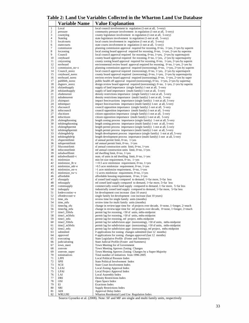
33

Table 2: Land Use Variables Collected in the Wharton Land Use Database Variable Name Value Explanation 1 Local local council involvement in regulation (1-not at all, 5-very) 2 pressure community pressure involvement in regulation (1-not at all, 5-very) 3 countyleg county legislature involvement in regulation (1-not at all, 5-very) 4 Stateleg state legislature involvement in regulation (1-not at all, 5-very) 5 localcourts local courts involvement in regulation (1-not at all, 5-very) 6 statecourts state courts involvement in regulation (1-not at all, 5-very) 7 commission planning commission approval required for rezoning, 0=no, 1=yes, 2=yes by superm 8 loczoning local zoning board approval required for rezoning, 0=no, 1=yes, 2=yes by superma 9 Council local council approval required for rezoning, 0=no, 1=yes, 2=yes by supermajorit 10 cntyboard county board approval required for rezoning, 0=no, 1=yes, 2=yes by supermajority 11 cntyzoning county zoning board approval required for rezoning, 0=no, 1=yes, 2=yes by superm 12 envboard environmental review board approval required for rezoning, 0=no, 1=yes, 2=yes by 13 commission_no~z planning commission approval required (norezoning), 0=no, 1=yes, 2=yes by superm 14 Council_norez local council approval required (norezoning), 0=no, 1=yes, 2=yes by supermajorit 15 cntyboard_norez county board approval required (norezoning), 0=no, 1=yes, 2=yes by supermajority 16 envboard_norez environ review board approval required (norezoning), 0=no, 1=yes, 2=yes by super 17 publhlth_norez public health off approval required (norezoning), 0=no, 1=yes, 2=yes by supermaj 18 dsgnrev_norez design review board approval required (norezoning), 0=no, 1=yes, 2=yes by superm 19 sfulandsupply supply of land importance (single family) 1-not at all, 5-very 20 mfulandsupply supply of land importance (multi family) 1-not at all, 5-very 21 sfudensrestr density restrictions importance (single family) 1-not at all, 5-very 22 mfudensrestr density restrictions importance (multi family) 1-not at all, 5-very 23 sfuimpact impact fees/exactions importance (single family) 1-not at all, 5-very 24 mfuimpact impact fees/exactions importance (multi family) 1-not at all, 5-very 25 sfucouncil council opposition importance (single family) 1-not at all, 5-very 26 mfucouncil council opposition importance (multi family) 1-not at all, 5-very 27 sfucitizen citizen opposition importance (single family) 1-not at all, 5-very 28 mfucitizen citizen opposition importance (multi family) 1-not at all, 5-very 29 sfulengthzoning length zoning process importance (single family) 1-not at all, 5-very 30 mfulengthzoning length zoning process importance (multi family) 1-not at all, 5-very 31 sfulengthpermit length permit process importance (single family) 1-not at all, 5-very 32 mfulengthpermit length permit process importance (multi family) 1-not at all, 5-very 33 sfulengthdvlp length development process importance (single family) 1-not at all, 5-very 34 mfulengthdvlp length development process importance (multi family) 1-not at all, 5-very 35 sfupermitlimit sf annual permit limit, 0=no, 1=yes 36 mfupermitlimit mf annual permit limit, 0=no, 1=yes 37 Sfuconstrlimit sf annual construction units limit, 0=no, 1=yes 38 mfuconstrlimit mf annual construction units limit, 0=no, 1=yes 39 mfudwelllimit mf dwelling limit, 0=no, 1=yes 40 mfudwellunitl~t num. of units in mf dwelling limit, 0=no, 1=yes 41 minlotsize min lot size requirement, 0=no, 1=yes 42 minlotsize_lh~e <=0.5 acre minlotsize requirement, 0=no, 1=yes 43 minlotsize_mh~e >0.5 acre minlotsize requirement, 0=no, 1=yes 44 minlotsize_on~e >1 acre minlotsize requirement, 0=no, 1=yes 45 minlotsize_tw~s >2 acres minlotsize requirement, 0=no, 1=yes 46 affordable affordable housing requirement, 0=no, 1=yes 47 sfusupply sf zoned land supply compared to demand, 1=far more, 5=far less 48 mfusupply mf zoned land supply compared to demand, 1=far more, 5=far less 49 commsupply commercially zoned land supply compared to demand, 1=far more, 5=far less 50 indsupply industrially zoned land supply compared to demand, 1=far more, 5=far less 51 lotdevcostinc~e lot development cost increase (last 10 years) 52 sflotdevcosti~e single family lot development cost increase (last 10 years) 53 time_sfu review time for single family units (months) 54 time_mfu review time for multi family units (months) 55 timechg_sfu change in review/appr time for sf projects over decade, 0=none, 1=longer, 2=much 56 timechg_mfu change in review/appr time for mf projects over decade, 0=none, 1=longer, 2=much 57 time1_l50sfu permit lag for rezoning, <50 sf units, mths-midpoint 58 time1_m50sfu permit lag for rezoning, >50 sf units, mths-midpoint 59 time1_mfu permit lag for rezoning, mf project, mths-midpoint 60 time2_l50sfu permit lag for subdivision appr (norezoning), <50 sf units, mths-midpoint 61 time2_m50sfu permit lag for subdivision appr (norezoning), >50 sf units, mths-midpoint 62 time2_mfu permit lag for subdivision appr (norezoning), mf project, mths-midpoint 63 submitted # applications for zoning changes submitted (last 12 months) 64 approved # applications for zoning changes approved (last 12 months) 65 execrating State Legislative Profile (Foster and Summers) 66 judicialrating State Judicial Profile (Foster and Summers) 67 town_meet Town Meeting for of Government 68 zonvote Town Meeting Aproves Zoning Changes 69 zonvote_super Town Meeting Aproves Zoning Changes by a Super-Majority 70 totinitiatives Total number of initiatives from 1996-2005 71 LPPI Local Political Pressure Index 72 SPII State Political Involvement Index 73 SCII State Court Involvement Index 74 LZAI Local Zoning Approval Index 75 LPAI Local Project Approval Index 76 LAI Local Assembly Index 77 DRI Density Restrictions Index 78 OSI Open Space Index 79 EI Exactions Index 80 SRI Supply Restrictions Index 81 ADI Approval Delay Index 82 WRLURI Wharton Residential Land Use Regulation Index

Source Gyourko et al. (2008). Note: SF and MF are single and multi family units, respectively

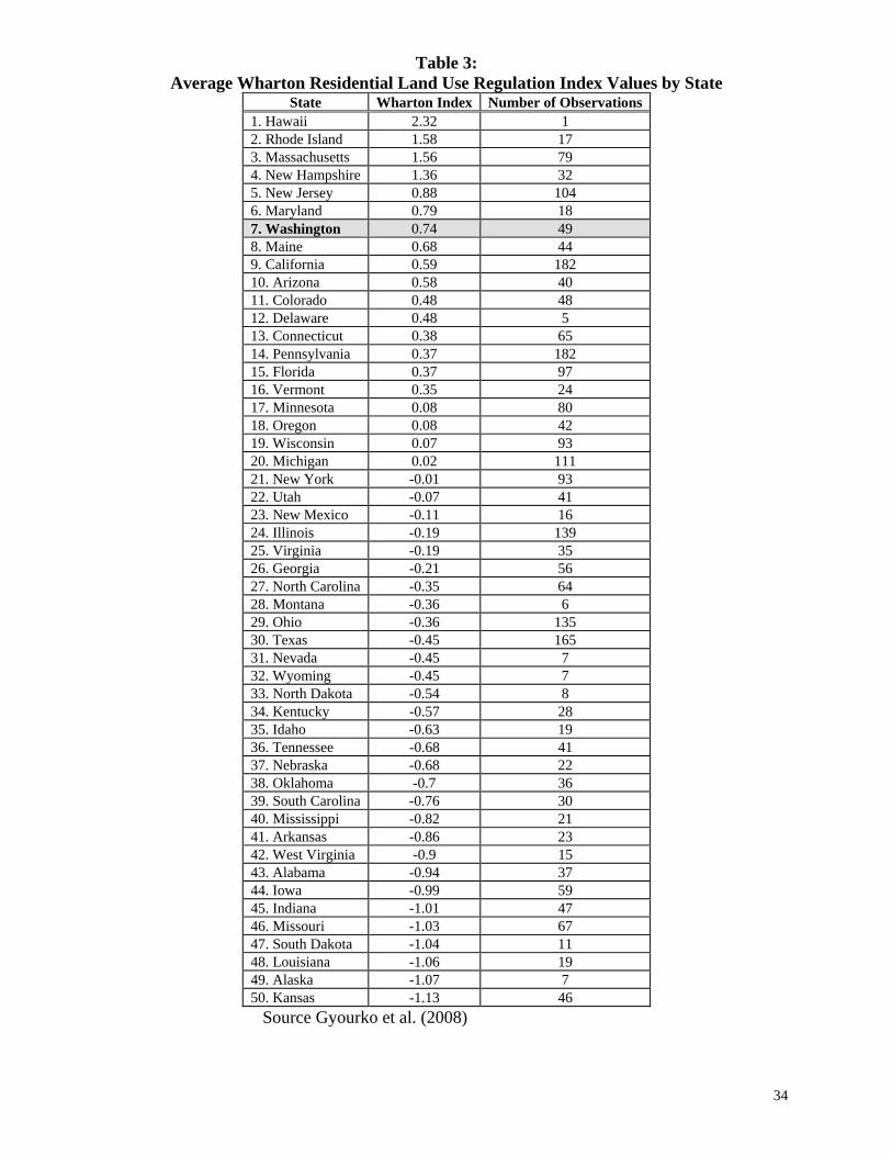
34

Table 3: Average Wharton Residential Land Use Regulation Index Values by State

State Wharton Index Number of Observations 1. Hawaii 2.32 1 2. Rhode Island 1.58 17 3. Massachusetts 1.56 79 4. New Hampshire 1.36 32 5. New Jersey 0.88 104 6. Maryland 0.79 18 7. Washington 0.74 49 8. Maine 0.68 44 9. California 0.59 182 10. Arizona 0.58 40 11. Colorado 0.48 48 12. Delaware 0.48 5 13. Connecticut 0.38 65 14. Pennsylvania 0.37 182 15. Florida 0.37 97 16. Vermont 0.35 24 17. Minnesota 0.08 80 18. Oregon 0.08 42 19. Wisconsin 0.07 93 20. Michigan 0.02 111 21. New York -0.01 93 22. Utah -0.07 41 23. New Mexico -0.11 16 24. Illinois -0.19 139 25. Virginia -0.19 35 26. Georgia -0.21 56 27. North Carolina -0.35 64 28. Montana -0.36 6 29. Ohio -0.36 135 30. Texas -0.45 165 31. Nevada -0.45 7 32. Wyoming -0.45 7 33. North Dakota -0.54 8 34. Kentucky -0.57 28 35. Idaho -0.63 19 36. Tennessee -0.68 41 37. Nebraska -0.68 22 38. Oklahoma -0.7 36 39. South Carolina -0.76 30 40. Mississippi -0.82 21 41. Arkansas -0.86 23 42. West Virginia -0.9 15 43. Alabama -0.94 37 44. Iowa -0.99 59 45. Indiana -1.01 47 46. Missouri -1.03 67 47. South Dakota -1.04 11 48. Louisiana -1.06 19 49. Alaska -1.07 7 50. Kansas -1.13 46

Source Gyourko et al. (2008)

35

Table 4: Wharton Residential Land Use Regulation Index Averages For Major Metropolitan Areas

Metropolitan Area Wharton Index Number of Observations 1 Providence-Fall River-Warwick 1.79 16 2 Boston 1.54 41 3 Monmouth-Ocean 1.21 15 4 Philadelphia 1.03 55 5 Seattle-Bellevue-Everett 1.01 21 6 San Francisco 0.9 13 7 Denver 0.85 13 8 Nassau-Suffolk 0.8 14 9 Bergen-Passaic 0.71 21 10 Fort Lauderdale 0.7 16 11 Phoenix-Mesa 0.7 18 12 New York 0.63 19 13 Riverside-San Bernardino 0.61 20 14 Newark 0.6 25 15 Springfield 0.58 13 16 Harrisburg-Lebanon-Carlisle 0.55 15 17 Oakland 0.52 12 18 Los Angeles-Long Beach 0.51 32 19 Hartford 0.5 28 20 San Diego 0.48 11 21 Orange County 0.39 14 22 Minneapolis-St 0.34 48 23 Washington DC 0.33 12 24 Portland-Vancouver 0.29 20 25 Milwaukee 0.25 21 26 Akron 0.15 11 27 Detroit 0.12 46 28 Allentown-Bethlehem-Easton 0.1 14 29 Chicago 0.06 95 30 Pittsburgh 0.06 44 31 Atlanta 0.04 26 32 Scranton-Wilkes-Barre-Hazelton 0.03 11 33 Salt Lake City-Ogden -0.1 19 34 Grand Rapids-Muskegon-Holland -0.15 16 35 Cleveland-Lorain-Elyria -0.16 31 36 San Antonio -0.17 12 37 Tampa-St. Petersburg-Clearwater -0.17 12 38 Houston -0.19 13 39 San Antonio -0.24 12 40 Fort Worth-Arlington -0.27 15 41 Dallas -0.35 31 42 Oklahoma City -0.41 12 43 Dayton-Springfield -0.5 17 44 Cincinnati OH-KY-IN -0.56 27 45 St. Louis MO-IL -0.72 27 46 Indianapolis IN -0.76 12 47 Kansas City MO-KS -0.8 29

Source Gyourko et al. (2008)

36

Figure 2 Simple Correlations between Housing Prices and Explanatory Variables

Figure 2a Figure 2b

Seattle city

-.02

0.0

2.0

4.0

6

-2 0 2 4

Wharton Regulatory Index

Ann

ual G

row

th In

Hou

sing

Pri

ces

Seattle city

-.02

0.0

2.0

4.0

6

-2 0 2 4

Seattle city

-.02

0.0

2.0

4.0

6

-2 0 2 4

Wharton Regulatory Index

Ann

ual G

row

th In

Hou

sing

Pri

ces

Seattle city

-.02

0.0

2.0

4.0

6

-.02 0 .02 .04

Income Growth

Ann

ual G

row

th In

Hou

sing

Pri

ces

Seattle city

-.02

0.0

2.0

4.0

6

-.02 0 .02 .04

Income Growth

Ann

ual G

row

th In

Hou

sing

Pri

ces

Figure 2c Figure 2d

Seattle city

-.02

0.0

2.0

4.0

6

-.05 0 .05 .1Population Growth

Ann

ual G

row

th In

Hou

sing

Pri

ces

Seattle city

-.02

0.0

2.0

4.0

6

-.05 0 .05 .1Population Growth

Ann

ual G

row

th In

Hou

sing

Pri

ces

Seattle city

-.02

0.0

2.0

4.0

6

0 20000 40000 60000Population Density

Ann

ual G

row

th In

Hou

sing

Pri

ces

Seattle city

-.02

0.0

2.0

4.0

6

0 20000 40000 60000Population Density

Ann

ual G

row

th In

Hou

sing

Pri

ces

37

Table 5: Regression Analysis Results

Dependent Variable:

Real Median Owner Occupied Housing Price Growth, 1989-2007

(1) (2) (3) Median Real Income Growth 0.549

(4.33)*** 0.455 (3.62)***

0.489 (4.00)***

Population Growth 0.172 (3.74)***

0.166 (3.65)***

0.149 (3.45)***

Density 6.66E-07 (3.72)***

6.19E-07 (3.52)***

4.81E-07 (2.73)***

Wharton Land Use Index

0.004 (3.95)***

Permit Approval Delays

0.00037 (1.6)*

Statewide Regulations

0.005 (3.85)***

Courts

0.004 (2.98)***

State Involvement in Local Land use and Growth Management

0.002 (2.54)**

Constant 0.019 (12.48)***

0.019 (12.34)***

-0.007 (1.62)

Observations 253 246 246 Adj. R-squared 0.21 0.25 0.33 Root MSE 0.0132 0.01288 0.01217 Variable definitions see Appendix 2; t statistics in parentheses; *, **, *** are 10%, 5%, 1% significance levels

Table 6: Sources of Real Housing Price Increase in Washington State

Seattle Tacoma Vancouver Everett Kent Housing Price in 20061 $447,800 $228,300 $233,600 $258,000 $281,600Real Housing Price Change 1989-06 102% 114% 137% 62% 62%

INCREASE IN HOUSING PRICES DUE TO: I) Common Factors Across Cities6 -$36,472 -$18,099 -$17,651 -$23,322 -$25,474II) Income & Population Growth $35,075 $8,382 $49,185 $7,343 $24,068III) Population Density $17,271 $5,099 $4,609 $4,968 $5,810IV) Land Use Restrictions/Regulations $203,525 $83,265 $73,086 $113,477 $124,614

IVa) Statewide Land Use Restrictions Imposed by Executive & Legislature2 $79,106 $39,256 $38,284 $50,584 $55,253

IVb) Municipal Land Use Restrictions Upheld by Courts3 $43,796 $21,733 $21,195 2800491% $30,589

IVc) Statewide Growth Management and Residential Building Restrictions4 $50,274 $19,958 $9,732 $25,718 $21,068

IVd) Approval Delay5

$30,350 $2,317 $3,874 $9,170 $17,704

Regulation % of 2006 Housing Price 45% 36% 31% 44% 44%1) For data sources see Appendix 2. 2) The level of activity in the Executive and Legislative branches over the past ten years that is directed toward enacting greater statewide land use restrictions. Source: Foster and Summers (2005) (execrating). 3) The tendency of appellate courts to uphold or restrain municipal land use regulation. Source: Foster and Summers (2005). 4) Involvement of state legislature in affecting residential building activities and/or growth management procedures Source: Gyourko et al. (2008) (stateleg). 5) Approval delay is the average time lag (in months) for a) relatively small, single-family projects involving fewer than 50 units; b) larger single-family developments with more than 50 units, and c) multifamily projects of indeterminate size. Lag times are due to the average duration of the review process, the time between application for rezoning and issuance of a building permit and the time between application for subdivision approval and the issuance of a building permit conditional on proper zoning being in place. Source: Gyourko et al. (2008). 6) Regression constant.

38

Appendix 1 Regression Diagnostics

If the regression model in equation (4) and its empirical implementation in Table 5 is missing vital explanatory variables, the coefficient estimates may be biased. Diagnostic tests exist to examine whether an explanatory variable may have been omitted, although it is systematically related to the variable of interest. Visual inspection of the residuals in Figure A1 shows a largely random pattern and provides no indication of an omitted explanatory variable (the R2 associated with Figure A1 is 0.0000). A more stringent test than the visual examination of the errors is to examine the normal probability plot for the residuals in Figure A2, to see whether the residuals are approximately normally distributed (e. g., random). Given Figure A2, it seems hard to argue that the residuals are not normally distributed. After ascertaining that there is no obvious evidence for omitted variable bias, it is important to examine the validity of the assumed functional form. Malpezzi (1996) proposes a nonlinear relationship between housing prices and regulations, which is suggested by the visual inspection of his data. Having extended his sample from about 50 to 250 major cities seems to have removed the apparent nonlinearity – at least according to a visual inspection of Figures 2a-d, which seem to indicate linear rather than nonlinear relationships. The STATA ovtest routine tests for omitted variables by examining alternative specifications of the baseline model that also feature polynomials. Adding polynomials for regulations does not improve the regression. The STATA reset test for regression specification errors (Ramsey 1969) also shows no evidence for nonlinearities in regulations in the sample of 250 cities. Malpezzi (1996) also used the log of housing price, presumably to address heteroskedasticity in his sample. The Breusch-Pagan tests for the constancy of the error variance; the obtained critical value indicates that the null hypothesis of homoskedasticity cannot be rejected.

Figure A1: Prediction Errors Figure A2: Residuals’ Normal Probability Plot

-.04

-.02

0.0

2.0

4R

esid

uals

0 .01 .02 .03 .04 .05

Fitted values

-.04

-.02

0.0

2.0

4R

esid

uals

0 .01 .02 .03 .04 .05

Fitted values

0.00

0.25

0.50

0.75

1.00

Stan

dard

Nor

mal

0.00 0.25 0.50 0.75 1.00

Empirical

The Residuals’ Normal Probability Plot compares the empirical cumulative distribution function of the Residuals with a theoretical standard normal distribution).

Appendix 2: Summary Statistics

Variable Description/Source Variable ID Observations Mean Std. Dev. Min Max Approval Delay Index Permit and Zoning Approval Delay

Index. See also Gyourko et al. (2008) adi 250 5.993556 3.784825 1.333333 29.38889

Executive and Legislative Rating

The level of activity in the executive and legislative branches over the past ten years that is directed toward enacting greater statewide land use restrictions. See Gyourko et al. (2008)

execrating 253 2.304348 .6888143 1 3

Real Housing Price 1989 housing prices (median owner occupied, 2006 dollars. Census) medval89_r 253 168220.2 105956 41132.74 570818.4

Housing Price 2006 housing prices (median owner occupied, 2006 dollars. Census) medval06 253 259140.3 169130.6 60900 806700

Real income growth Average annual compound growth of real median household income 1989-2006 (Census, 2006 dollars)

mi_gr 253 -.0024926 .0075162 -.0235441 .0350843

Real Housing Price Growth

Average annual compound growth of the real price of the median owner occupied house 1989-2006 (2006 dollars, Census).

mv_gr 253 .0234268 .0148009 -.0256737 .0683899

Density 2006 Population (Census) / 2000 Land area (Census) person_sqm06 253 4521.534 4765.727 164.2102 53347.4

Population growth Average annual compound growth of the population 1989-2006. (Census) pop_gr 253 .0150111 .0210629 -.0140978 .1097826

State Court Involvement Index

Judicial land use environment. Tendency of courts to uphold or restrain municipal land-use regulations See Gyourko et al. (2008)

scii 253 2.245059 .593638 1 3

State Legislature Involvement

The degree of involvement of the state legislature in affecting the residential building activities and/or growth management procedures of a jurisdiction. See Gyourko et al. (2008)

stateleg 247 2.194332 1.068149 1 5

Wharton Residential Land Use Regulatory Index (“Wharton Index”)

See Gyourko et al. (2008) wrluri 246 .0779213 .9386766 -1.9241 3.625351

The dataset is the Wharton Dataset (Gyourko et al., 2008, downloaded 07/02/07) merged with the 1990 Census data (1990 census place data for entire nation (nation file), which contains places of 10,000+ inhabitants obtained from the UW Center for Social Science Computation and Research (CSSCR)) and 2006 Census Data (Public Use Microdata Sample (PUMS), downloaded from AmericanFactfinder.com). Land Area was obtained from the 2000 Census Tiger Gazetteer database. Real variables are adjusted for inflation (and expressed in 2006 dollars) using the consumer price index, http://www.bls.gov/cpi/. “Appleton WI” was deleted in the Wharton data; the city of ~70000 inhabitants was found to have two entries in the Wharton database with different land use restrictions (this explains slightly different results as in the previous version of the paper. Cost estimates = (regressor* coef)/mv_gr * (medval06-medval89_r).

40

Appendix 3 Stringency of Land Use Regulations in the Wharton Sample for Washington State

(As Reported by City Planning Directors to Wharton)

A 99 percent ranking indicates that less than 1 percent of the cities in the sample (or 27 of 2729 cities) feature more stringent regulations in that particular category. Source: Gyourko et al. (2008). Note: All Washington cities included in Appendix 3, but excluded in the regressions had to be dropped because of insufficient Census data. Data labels are provided in Table 2. Empty cells indicate the data is not available.

City rank

_wrl

uri

rank

_sta

teco

urts

rank

_sta

tele

gra

nk_a

dira

nk_t

ime_

mfu

rank

_tim

e1_m

fura

nk_t

ime2

_mfu

rank

_tim

e1_m

50sf

ura

nk_t

ime2

_m50

sfu

rank

_tim

e_sf

ura

nk_t

ime1

_l50

sfu

rank

_tim

e2_l

50sf

ura

nk_l

ppi

rank

_pre

ssur

era

nk_d

sgnr

ev_n

orez

rank

_env

boar

d_no

rez

rank

_tot

initi

ativ

esra

nk_s

fula

ndsu

pply

rank

_sfu

supp

lyra

nk_l

ocal

cour

tsra

nk_c

ount

yleg

rank

_sfu

leng

thpe

rmit

rank

_mfu

leng

thpe

rmit

rank

_exe

crat

ing

rank

_osi

rank

_mfu

citiz

enra

nk_m

inlo

tsiz

e_m

halfa

cre

rank

_cou

ncil_

nore

zra

nk_s

fuco

unci

lra

nk_s

fuim

pact

rank

_mfu

impa

ctra

nk_s

fule

ngth

zoni

ngra

nk_s

fule

ngth

dvlp

rank

_mfu

leng

thzo

ning

rank

_mfu

budg

etra

nk_m

fule

ngth

dvlp

rank

_sfu

budg

etra

nk_m

fuco

unci

lra

nk_s

fusc

hool

rank

_mfu

scho

olra

nk_m

fuin

frac

ost

rank

_sfu

infr

acos

tra

nk_m

fula

ndsu

pply

rank

_sfu

citiz

enra

nk_l

zai

rank

_mfu

supp

lyra

nk_s

fude

nsre

str

rank

_ind

supp

lyra

nk_p

ublh

lth_n

orez

rank

_com

msu

pply

rank

_lot

devc

ostin

crea

sera

nk_s

flotd

evco

stin

crea

sera

nk_t

imec

hg_s

fura

nk_t

imec

hg_m

fu

Seattle 98% 99% 98% 97% 93% 92% 94% 91% 93% 91% 94% 96% 97% 95% 90% 97% 98% 39% 45% 28% 25% 26% 25% 78% 73% 32% 31% 28% 24% 22% 22% 22% 21% 21% 21% 21% 20% 20% 20% 19% 19% 18% 14% 14% 13% 11% 10% 52% 45% 3% Buckley 98% 65% 92% 89% 71% 92% 80% 91% 77% 79% 94% 83% 91% 95% 90% 47% 45% 74% 45% 28% 84% 64% 63% 78% 73% 76% 81% 77% 88% 90% 89% 58% 55% 55% 94% 54% 95% 81% 73% 70% 64% 62% 75% 86% 13% 36% 71% 52% 45% 47% 64% 67% 33% 32%University 98% 96% 92% 89% 27% 92% 80% 91% 93% 13% 94% 83% 96% 42% 41% 47% 93% 39% 45% 70% 63% 64% 83% 78% 73% 93% 77% 76% 76% 75% 93% 77% 91% 51% 76% 51% 94% 73% 85% 39% 38% 14% 86% 13% 92% 71% 52% 45% 82% 64% 67% 33% 96%Sammamish 97% 96% 92% 95% 86% 92% 94% 91% 93% 73% 94% 96% 77% 75% 41% 47% 45% 74% 5% 97% 63% 26% 25% 78% 73% 93% 28% 96% 22% 22% 22% 21% 21% 21% 21% 20% 94% 73% 70% 6% 6% 5% 96% 1% 2% 10% 96% 45% 3% 33% 32%Kent 94% 87% 76% 93% 8% 92% 94% 91% 93% 13% 94% 96% 89% 95% 90% 97% 45% 74% 45% 90% 84% 94% 93% 78% 73% 76% 31% 28% 96% 97% 97% 93% 91% 91% 51% 90% 51% 94% 87% 85% 87% 87% 75% 86% 97% 69% 90% 19% 45% 47% 95% 91% 33% 32%Sumner 94% 96% 98% 93% 27% 92% 94% 91% 93% 13% 94% 96% 67% 75% 90% 47% 45% 74% 45% 70% 99% 26% 25% 78% 73% 54% 31% 77% 76% 22% 22% 22% 55% 21% 21% 54% 20% 67% 20% 19% 64% 62% 75% 66% 13% 36% 10% 52% 45% 15% 11% 91% 81% 78%Burlington 93% 87% 76% 49% 64% 42% 51% 39% 47% 73% 48% 55% 93% 75% 90% 47% 45% 74% 93% 97% 94% 98% 98% 78% 73% 93% 81% 28% 96% 97% 97% 98% 97% 97% 83% 97% 83% 94% 96% 95% 87% 87% 75% 96% 50% 92% 90% 52% 45% 47% 38% 30% 33% 32%Issaquah 93% 87% 92% 95% 64% 92% 94% 91% 99% 13% 94% 96% 71% 75% 90% 47% 45% 74% 45% 28% 84% 26% 25% 78% 73% 54% 28% 76% 76% 75% 22% 55% 21% 69% 54% 69% 67% 52% 50% 19% 18% 75% 66% 13% 36% 29% 52% 45% 47% 33% 32%Olympia 92% 87% 76% 94% 49% 92% 51% 99% 93% 59% 100% 96% 90% 75% 41% 47% 93% 39% 45% 90% 63% 64% 83% 78% 73% 32% 28% 58% 90% 89% 22% 77% 21% 51% 90% 51% 20% 73% 50% 39% 62% 26% 66% 50% 11% 71% 82% 45% 15% 79% 67% 33% 32%Kirkland 91% 87% 98% 96% 93% 92% 94% 91% 93% 59% 94% 96% 86% 75% 90% 47% 93% 74% 93% 70% 63% 84% 83% 78% 23% 54% 31% 28% 24% 55% 54% 22% 55% 55% 21% 76% 20% 67% 20% 19% 19% 18% 75% 14% 50% 36% 29% 19% 45% 47% 87% 91% 81% 78%Des Moines 90% 25% 49% 53% 64% 74% 16% 70% 14% 37% 79% 18% 92% 3% 41% 47% 93% 39% 93% 28% 25% 98% 98% 78% 73% 54% 81% 28% 96% 97% 75% 98% 97% 97% 94% 97% 95% 94% 20% 19% 64% 87% 41% 14% 13% 92% 90% 52% 45% 15% 64% 67% 98% 96%Ponlsbo 89% 99% 92% 95% 49% 92% 51% 99% 93% 93% 100% 96% 56% 42% 41% 47% 45% 74% 75% 90% 84% 84% 63% 78% 23% 32% 81% 77% 58% 76% 75% 58% 91% 55% 69% 76% 69% 49% 52% 50% 39% 62% 26% 41% 50% 36% 49% 82% 45% 47% 64% 67% 81% 32%Covington 89% 87% 76% 89% 71% 92% 80% 91% 77% 79% 94% 83% 62% 75% 41% 47% 45% 74% 75% 70% 94% 84% 83% 78% 73% 32% 31% 28% 58% 55% 54% 81% 77% 78% 21% 76% 20% 49% 73% 70% 19% 18% 75% 41% 13% 69% 10% 82% 95% 82% 87% 77% 33% 32%Redmond 87% 87% 92% 90% 79% 74% 80% 91% 93% 13% 94% 96% 41% 75% 90% 47% 45% 74% 75% 90% 94% 64% 63% 78% 73% 32% 28% 24% 76% 75% 58% 77% 55% 51% 76% 51% 20% 20% 19% 64% 62% 75% 41% 50% 36% 71% 19% 45% 47% 87% 77% 33% 32%Auburn 87% 65% 76% 91% 64% 92% 94% 91% 93% 73% 79% 83% 28% 42% 41% 47% 45% 39% 45% 90% 63% 64% 63% 78% 73% 76% 31% 77% 24% 76% 75% 58% 55% 55% 21% 54% 20% 20% 20% 19% 39% 38% 41% 41% 13% 36% 29% 52% 45% 47% 64% 77% 33% 32%Mercer Island 86% 87% 92% 91% 71% 92% 94% 91% 93% 73% 79% 83% 94% 95% 41% 47% 93% 74% 75% 70% 84% 64% 63% 78% 23% 54% 28% 58% 55% 54% 58% 55% 55% 51% 54% 51% 49% 52% 50% 39% 38% 75% 66% 50% 36% 71% 52% 45% 47% 64% 67% 33% 32%Cheney 85% 87% 98% 88% 64% 92% 80% 91% 77% 73% 94% 83% 74% 75% 41% 47% 45% 39% 45% 90% 84% 84% 83% 78% 73% 54% 31% 28% 24% 90% 89% 93% 77% 91% 83% 76% 83% 49% 73% 70% 64% 62% 41% 66% 50% 11% 71% 4% 45% 82% 81% 78%Milton 84% 96% 98% 84% 64% 92% 51% 91% 77% 37% 94% 55% 81% 75% 41% 47% 45% 39% 45% 97% 84% 94% 93% 78% 23% 93% 31% 77% 24% 90% 89% 81% 91% 78% 94% 90% 95% 94% 20% 19% 19% 18% 75% 96% 50% 92% 90% 19% 45% 15% 11% 30% 33% 32%Woodland 83% 65% 76% 80% 79% 74% 51% 91% 77% 85% 79% 55% 35% 75% 41% 47% 45% 39% 75% 28% 63% 94% 93% 78% 73% 32% 77% 58% 22% 22% 81% 91% 78% 21% 90% 20% 49% 52% 50% 39% 38% 41% 41% 50% 36% 49% 19% 45% 47% 79% 67% 81% 78%Kenmore 83% 65% 49% 59% 89% 42% 51% 39% 47% 85% 48% 55% 35% 75% 41% 47% 45% 74% 75% 28% 63% 84% 83% 78% 73% 32% 81% 28% 58% 76% 75% 81% 77% 78% 21% 76% 20% 49% 20% 19% 64% 62% 75% 41% 13% 36% 71% 52% 45% 47% 38% 67% 81% 78%Snohomish 82% 25% 17% 84% 71% 92% 51% 91% 47% 73% 94% 55% 67% 75% 90% 47% 45% 74% 45% 70% 25% 26% 83% 78% 23% 12% 81% 77% 58% 55% 54% 58% 21% 55% 83% 54% 83% 49% 87% 85% 87% 87% 14% 66% 99% 11% 49% 82% 45% 3% 38% 52% 33% 32%Seatac 81% 87% 92% 47% 49% 74% 51% 70% 14% 13% 48% 18% 45% 75% 41% 47% 45% 39% 75% 28% 94% 26% 63% 78% 73% 32% 81% 28% 24% 22% 22% 22% 21% 55% 51% 54% 20% 49% 20% 19% 39% 18% 41% 14% 13% 11% 10% 96% 45% 82% 64% 67% 33% 32%Kennewick 81% 87% 92% 44% 49% 42% 51% 39% 47% 59% 48% 55% 41% 42% 41% 47% 45% 24% 45% 70% 63% 26% 25% 78% 73% 54% 81% 28% 58% 55% 54% 22% 21% 21% 21% 21% 20% 81% 20% 19% 64% 62% 41% 66% 13% 69% 29% 82% 45% 47% 38% 30% 81% 78%Lake Stevens 81% 87% 76% 68% 71% 74% 51% 70% 47% 79% 79% 55% 45% 42% 90% 47% 45% 39% 93% 28% 25% 26% 25% 78% 73% 32% 31% 77% 24% 90% 89% 22% 21% 21% 83% 21% 83% 49% 52% 50% 19% 38% 41% 41% 50% 69% 49% 52% 45% 82% 64% 67% 81% 78%Washougal 77% 65% 76% 84% 8% 11% 16% 91% 93% 59% 94% 96% 67% 42% 41% 47% 45% 39% 45% 70% 94% 26% 78% 23% 32% 28% 58% 76% 22% 77% 83% 83% 49% 52% 50% 87% 41% 50% 36% 71% 19% 45% 47% 81% 78%Fircrest 76% 87% 92% 70% 64% 42% 51% 70% 77% 73% 79% 83% 49% 42% 41% 47% 45% 39% 75% 90% 84% 26% 25% 78% 73% 76% 31% 28% 58% 22% 22% 22% 21% 21% 21% 21% 20% 81% 20% 19% 39% 62% 75% 41% 50% 36% 49% 19% 45% 47% 79% 77% 33% 32%Port Townsend 74% 65% 92% 80% 27% 92% 51% 91% 47% 13% 94% 55% 38% 95% 90% 97% 45% 5% 5% 70% 63% 26% 25% 78% 23% 32% 28% 24% 22% 22% 58% 21% 21% 21% 54% 20% 49% 20% 19% 19% 62% 26% 41% 50% 36% 10% 19% 45% 47% 11% 77% 33% 78%Liberty Lake 73% 65% 49% 33% 8% 42% 51% 39% 47% 13% 48% 55% 56% 42% 41% 47% 45% 74% 45% 70% 63% 26% 25% 78% 73% 54% 31% 77% 76% 55% 54% 22% 21% 21% 21% 21% 20% 67% 87% 85% 64% 62% 41% 66% 50% 36% 49% 52% 45% 47% 95% 91% 33% 32%Centralia 73% 99% 98% 38% 49% 42% 51% 39% 47% 13% 48% 55% 96% 95% 41% 47% 45% 5% 100% 99% 78% 23% 93% 31% 28% 96% 94% 95% 94% 73% 70% 96% 50% 2% 4% 95% 3% 81% 78%Normandy Park 72% 65% 76% 67% 27% 74% 80% 70% 77% 13% 79% 55% 59% 42% 41% 47% 45% 74% 93% 70% 25% 64% 63% 78% 23% 93% 81% 28% 88% 55% 54% 58% 55% 55% 21% 54% 20% 81% 52% 50% 19% 18% 75% 86% 50% 69% 71% 95% 47% 38% 77% 33% 32%Lakewood, 72% 65% 76% 74% 71% 74% 80% 70% 77% 59% 48% 83% 88% 42% 41% 47% 93% 74% 75% 70% 94% 84% 83% 78% 23% 54% 31% 28% 24% 22% 22% 81% 55% 78% 21% 54% 20% 20% 52% 50% 64% 62% 75% 14% 50% 11% 29% 19% 45% 47% 87% 77% 33% 32%Port Orchard 71% 96% 98% 74% 79% 42% 80% 70% 77% 85% 48% 83% 41% 42% 41% 47% 45% 74% 75% 90% 94% 64% 63% 78% 73% 32% 28% 58% 55% 54% 58% 55% 55% 21% 54% 20% 49% 52% 50% 39% 38% 26% 41% 50% 36% 49% 82% 45% 47% 38% 52% 81% 78%Squim 71% 96% 76% 48% 49% 11% 16% 39% 14% 59% 14% 96% 28% 75% 41% 47% 45% 74% 45% 97% 25% 26% 25% 78% 73% 54% 31% 77% 24% 22% 22% 58% 55% 55% 21% 54% 20% 20% 20% 19% 19% 62% 14% 66% 50% 69% 90% 96% 45% 47% 38% 67% 33% 32%Everett, 71% 87% 92% 74% 49% 74% 80% 70% 77% 37% 79% 83% 41% 42% 41% 47% 45% 74% 93% 70% 99% 26% 25% 78% 73% 12% 28% 24% 22% 22% 22% 55% 21% 21% 54% 20% 20% 73% 70% 39% 38% 75% 14% 50% 36% 10% 52% 45% 3% 64% 91% 33% 32%Raymond, 67% 87% 98% 3% 8% 11% 16% 10% 14% 13% 14% 18% 81% 42% 41% 47% 45% 5% 17% 90% 99% 64% 78% 73% 32% 77% 76% 55% 58% 55% 94% 95% 67% 52% 50% 38% 41% 50% 11% 10% 19% 45% 15% 11% 9% 33% 32%Arlington 67% 87% 76% 54% 49% 42% 51% 70% 77% 13% 48% 55% 28% 42% 90% 47% 45% 74% 93% 90% 94% 26% 25% 78% 73% 12% 28% 24% 22% 22% 22% 21% 21% 21% 21% 20% 20% 20% 19% 19% 18% 75% 14% 50% 92% 10% 19% 45% 15% 11% 9% 33% 32%East Wenatchee 63% 99% 92% 44% 49% 42% 51% 39% 47% 59% 48% 55% 62% 75% 41% 47% 45% 14% 17% 90% 99% 26% 25% 78% 23% 54% 77% 24% 22% 22% 22% 21% 21% 21% 21% 20% 20% 52% 50% 87% 87% 41% 66% 50% 69% 29% 52% 45% 82% 38% 30% 33% 32%Woodinville 60% 99% 76% 69% 64% 74% 80% 39% 77% 59% 48% 83% 1% 3% 41% 47% 45% 74% 75% 97% 63% 26% 25% 78% 73% 12% 31% 28% 24% 22% 22% 22% 21% 21% 21% 21% 20% 20% 20% 19% 64% 62% 75% 14% 1% 36% 10% 52% 45% 47% 38% 52% 33% 32%Pullman 59% 25% 17% 58% 27% 42% 80% 39% 77% 13% 48% 83% 15% 16% 41% 47% 45% 39% 75% 28% 84% 26% 25% 78% 23% 32% 77% 58% 22% 22% 22% 21% 21% 21% 21% 20% 49% 20% 19% 19% 18% 14% 41% 50% 11% 29% 52% 45% 47% 38% 52% 33% 32%Vancouver 57% 65% 49% 44% 49% 42% 51% 39% 47% 59% 48% 55% 21% 75% 41% 47% 45% 74% 75% 28% 25% 26% 25% 78% 73% 54% 31% 28% 24% 90% 89% 58% 21% 55% 21% 21% 20% 20% 20% 19% 64% 62% 75% 14% 13% 36% 10% 52% 45% 15% 64% 52% 33% 32%Bremerton 55% 65% 76% 59% 27% 74% 51% 70% 77% 37% 48% 55% 31% 42% 41% 47% 45% 39% 75% 28% 63% 26% 25% 78% 23% 54% 31% 28% 24% 22% 22% 22% 55% 55% 21% 54% 20% 20% 52% 50% 6% 6% 26% 41% 50% 36% 10% 19% 95% 15% 64% 67% 33% 32%Ephrata 51% 87% 92% 57% 49% 74% 51% 70% 47% 59% 48% 55% 13% 42% 41% 47% 45% 14% 45% 70% 25% 64% 63% 78% 23% 54% 31% 77% 24% 22% 22% 81% 97% 91% 21% 90% 20% 20% 20% 19% 19% 62% 5% 41% 13% 92% 71% 4% 45% 82% 11% 9% 81% 78%Chehalis 48% 99% 98% 44% 8% 74% 16% 70% 14% 13% 79% 18% 49% 95% 41% 47% 45% 74% 93% 70% 99% 64% 63% 78% 23% 12% 31% 28% 24% 22% 22% 81% 55% 78% 21% 54% 20% 20% 20% 19% 64% 62% 75% 14% 13% 69% 29% 82% 45% 47% 38% 30% 33% 32%Lacey 45% 87% 76% 60% 64% 42% 51% 70% 77% 73% 48% 55% 28% 42% 41% 47% 45% 5% 45% 90% 94% 26% 25% 78% 23% 12% 31% 28% 24% 22% 22% 22% 21% 21% 21% 21% 20% 20% 20% 19% 6% 6% 5% 14% 50% 11% 10% 52% 45% 47% 38% 52% 81% 32%Forks 44% 96% 49% 13% 49% 11% 16% 10% 14% 59% 14% 18% 2% 42% 41% 47% 45% 14% 5% 70% 63% 26% 25% 78% 73% 12% 31% 28% 24% 22% 22% 22% 21% 21% 21% 21% 20% 20% 20% 19% 64% 62% 14% 14% 50% 2% 29% 52% 95% 47% 11% 30% 33% 32%Chelan 40% 25% 76% 33% 8% 42% 51% 39% 47% 13% 48% 55% 35% 75% 41% 47% 45% 14% 17% 28% 25% 26% 25% 78% 23% 32% 31% 28% 58% 22% 22% 22% 21% 21% 51% 21% 51% 49% 20% 19% 64% 62% 14% 41% 50% 11% 10% 19% 45% 15% 64% 52% 33% 32%Tacoma 30% 87% 92% 17% 8% 42% 16% 39% 14% 13% 48% 18% 13% 16% 41% 47% 45% 74% 45% 70% 84% 26% 25% 78% 23% 54% 31% 28% 24% 22% 22% 22% 21% 21% 21% 21% 20% 20% 20% 19% 19% 18% 75% 41% 13% 11% 10% 19% 45% 15% 11% 9% 33% 32%Burien 28% 65% 49% 30% 49% 11% 51% 10% 47% 37% 48% 55% 2% 16% 41% 47% 45% 74% 17% 70% 25% 26% 25% 78% 23% 12% 31% 28% 24% 22% 22% 22% 21% 21% 21% 21% 20% 20% 20% 19% 6% 6% 75% 14% 13% 11% 10% 19% 45% 15% 33% 32%Aberdeen 23% 25% 17% 3% 8% 11% 16% 10% 14% 13% 14% 18% 7% 16% 41% 47% 45% 74% 5% 28% 25% 98% 98% 78% 23% 12% 31% 28% 24% 22% 22% 98% 97% 97% 21% 97% 20% 20% 20% 19% 87% 87% 75% 14% 50% 2% 10% 4% 45% 3% 11% 9% 33% 32%Shoreline 87% 49% 38% 64% 11% 16% 39% 47% 73% 48% 55% 41% 95% 45% 74% 93% 70% 63% 26% 25% 78% 23% 12% 31% 24% 22% 22% 22% 21% 21% 69% 21% 69% 20% 20% 19% 87% 87% 75% 14% 50% 92% 71% 96% 96% 33% 32%

41

Appendix 3 Table A3.1

Results From Comparative Studies of Land Use Restrictions and Housing Prices Study

Authors Year Cities/Regions Effects

1 Anthony 2006 FL Increase in prices attributable to statewide growth

management. 2 Glaeser, Schuetz,

Ward 2006 187 Communities

in Eastern MA 23-36 percent increase in prices (about $156,000) due to regulations.

3 Somerville / Meyer

2006 44 Metro Areas 20% higher price elasticities and 45% lower housing starts in more regulated areas.

4 Xing et al. 2006 54 Metro Areas Increase in prices due to growth management and development restrictiveness. Seattle: 15% increase in prices due to growth management tools

5 Chan 2004 97 Metro Areas 44.8% to -3.9% increases in price in cities with urban growth boundaries.

6 Downs 2002 86 Metro Areas Increase in prices 1990-2000, 1990-94, 1990-96 due to Urban Growth Boundary. Not significant 1994-2000, 1996-2000, so UGB increases housing prices combined with stimulated housing demand.

7 Glaeser/Gyourko 2002 40 Metro Areas $50-$700,000 increase in prices due to zoning restrictions. (Seattle: +$200,000)

8 Malpezzi 2002 55 Metro Areas Increase in prices due to regulations, controlling for High Tech Locations

9 Staley/Gilroy 2001 OR, FL, WA 15% increase in prices attributed to growth management.

10 Luger/Temkin 2000 NC, NJ $40-80,000 increase in prices of new homes due to regulations

11 Phillips et al 2000 37 Metro Areas Increase in prices due to regulation index and weak evidence for urban growth boundary effect. But impact is low (less than $10,000 per unit).

12 Green 1999 Waukesha, WI 8% increase in prices due to zoning and permitting restrictions

13 Malpezzi, et al. 1998 55 Metro Areas 9-46% increase in prices due to regulations 14 Malpezzi 1996 60 Metro Areas 51% increase in prices due to regulations 15 Thorson 1996 10 Metro Areas Increase in prices due to “zoning monopolies” 16 Cho/Linneman 1993 Fairfax, VA Increase in prices due to minimum lot sizes.

No increase in prices due to residential restrictions 17 Downs 1992 San Diego, CA 54% increase in prices due to growth management 18 Pollakowski/

Wachter 1990 Montgomery, MD 27% increase in prices (price elasticity: 0.275) due

to regulatory restrictiveness 19 Katz/Rosen 1987/1 63 CA Metros 17-38% increase in prices due to growth

management 20 Landis 1986 CA 35-45% increase in prices in growth controlled

areas 21 Schwartz et al. 1986 Sacramento,

Davis 9% increase in prices due to growth controls

22 Segal/ Srinivasan 1985 51 Metro Areas 20% increase in prices in growth restricted areas Sources: Original sources, Lillydahl and Singell (1987), Pogodzinski and Sass, 1991, Ihlanfeldt (2004), Xing et al.(2006), Landis et al.(2002), and Quigley and Rosenthal (2005). Table surveys studies that included a substantial number of cities or metropolitan areas with significant effects.

42

Table A3.2 Empirical Studies on the Impact of Growth Regulation on Housing Prices

Surveyed by Nelson et al. (2004) Study Authors Year Cities/Regions Impact? Luger and Temkin 2000 New Jersey, North Carolina Yes Green 1999 Suburban Wisconsin Yes Porter et al. 1996 Montgomery County, Maryland Yes Beaton and Pollock 1992 Chesapeake Bay, Maryland Yes Downs 1992 San Diego County Yes Parsons 1992 Chesapeake Bay, Maryland Yes Beaton 1991 New Jersey Pinelands Yes Guidry, Shilling, and Sirmans 1991 National Yes Shilling 1991 National Yes Dale-Johnson and Kim 1990 California Coast Yes Pollakowski and Wachter 1990 Montgomery County, Maryland Yes Rose 1989 National Yes Chambers and Diamond 1988 National Yes Nelson 1988 Washington County, Oregon Yes Katz and Rosen 1987 San Francisco Bay Area Yes Landis 1986 Sacramento, Fresno, San Jose, California Yes Nelson 1986 Salem, Oregon Yes Zorn et al. 1986 Davis, California Yes Black and Hoben 1985 National Yes Knaap 1985 Portland, Oregon Yes Segal and Srinivasan 1985 National Yes Dowall 1984 Santa Rosa, Napa, California Yes Frech and Lafferty 1984 California Coast Yes Dowall and Landis 1982 San Francisco Bay Area Yes Mercer and Morgan 1982 Santa Barbara County, California Yes Schwartz et al. 1981, 84 Petaluma, Santa Rosa, Rohnert Park, CA Yes Elliot 1981 California Yes Correll, Lillydahl, and Singell 1978 Boulder, Colorado Yes Real Estate Research Corp 1978 St. Louis County, Missouri Yes Urban Land Institute 1977 National Yes Richardson 1976 Dover Township, New Jersey Yes Peterson 1973 Fairfax County, Virginia Yes Phillips and Goodstein 2000 Portland, Oregon No Glickfield and Levine 1992 California No Knaap and Nelson 1992 Portland, Oregon No Landis 1992 California No Downs 2002 Portland, Oregon Mixed Lowry and Ferguson 1992 Sacramento, Orlando, Nashville Mixed Miller 1986 Boulder, Colorado Mixed Gleeson 1978 Brooklyn Park, Minnesota Mixed Source: Connerly (2004), see the original paper for full citations.