how active could passive hedge fund management be?

1

How Active Could Passive Hedge Fund Management Be?

Jun Duanmu1, Alexey Malakhov

2, and William R. McCumber

3

This draft: April, 2012

ABSTRACT

Hedge funds are considered the apex of active portfolio management. We identify two distinct styles of active

portfolio management: traditionally active, wherein managers do not follow any particular benchmarks, and

passively active, wherein managers follow identifiable benchmark factors. The latter choose benchmark factors in

anticipation of changing economic conditions and opportunity sets. We articulate that traditional measures of

superior active performance, such as positive alpha and low R2 over relatively short time periods, do not provide

adequate information as to managerial performance on behalf of fund investors. We construct alternative measures

that allow us to quantify both the existence and also the success of passively active portfolio management. We find

ample evidence that passively active managers deliver superior contemporaneous as well as subsequent

performance.

JEL classification: G12, G23

Keywords:

Hedge funds, active management, passive management, performance measurement

1 Jun Duanmu, [email protected], 479-575-4505, Walton College of Business, University of Arkansas,

WCOB 302, Fayetteville, Arkansas 72701, United States of America. 2 Alexey Malakhov, [email protected], 479-575-6118, Walton College of Business, University of

Arkansas, WCOB 302, Fayetteville, Arkansas 72701, United States of America. 3 William R. McCumber, [email protected], Walton College of Business, University of Arkansas,

WCOB 302, Fayetteville, Arkansas 72701, United States of America. Phone: 1-479-856-9639, Fax: 1-479-575-

8407.

mailto:[email protected]



2

1. Introduction

Hedge funds are considered the apex of professionally actively managed investment funds.

Hedge fund researchers commonly speak of alpha, the coefficient on the constant in a regression

specified by an asset pricing model, as a proxy for fund performance due to active portfolio

management. Fund excess returns, or returns minus a risk-free asset, are regressed against factor

returns. In essence, alpha is the performance of a fund that cannot be explained by the model,

and therefore positive alpha is a proxy for positive outperformance, at least compared to the

factor returns, whereas negative alpha is a proxy for poor performance; i.e. the investor would

have enjoyed a higher return over the period by passively holding the factors. Alpha is firmly

entrenched in the common investment lexicon as a sophisticated measure of performance; fund

managers, investment advisors, and investors all are “seeking alpha”.

However, alpha is not a reliable measure of fund performance. Alpha changes depending on

the model specification. What are the relevant factors? Factor models are now ubiquitous in the

literature, and all model specifications and even the same model specification over different time

periods will necessarily produce different alpha estimations. Past alpha is not necessarily

predictive of future alpha or performance. Further, investors cannot put alpha in their pockets.

Alpha is not realized, fund returns are. A fund may be performing very well by investor

standards – actual returns – while statistically alpha may be zero or even negative. What does

this mean? To date, there are no universally agreed-upon or intuitive means to define adequate

hedge fund performance, active management (for which investors are paying hefty fees), or

reasonably predict future active management or performance. How are investors and advisors to

pick funds? The global hedge fund industry is seemingly recovered from the outflows of the

3

financial crisis of 2007-2008. Total industry assets under management reached well over $2

trillion in the first quarter of 2011, with fund flows4 of $102 billion in that quarter alone. It is

therefore important to investors and the financial system to better understand the nature of hedge

fund managerial activity and performance.

In this paper we define two styles of active management of hedge funds, which are

‘traditionally active’ and ‘passively active’. Traditionally, active management has been identified

by the low R2 from a regression. Borrowing from Sharpe (1992), we define ‘traditionally active’

management such that manager positions are not ultimately reflected in factor loadings. For

example, a traditional long-short stock picker should have a low R2 as the variance in factor

returns should not explain fund returns. If a manager is skilled, the alpha should be positive and

significant, reflecting superior returns as compared to passively holding factor-mimicking

portfolios. By this traditional definition, high R2 funds are passively managed, whereas low R

2

funds are actively managed in that investors could not easily replicate the fund’s performance by

holding passive investments.

However, generating superior alpha is not the goal in itself, as the ultimate goal of successful

active portfolio management is to generate consistently superior returns to the investor over a

long period of time. This objective can also be achieved by market timing via successfully

following the factors generating the highest absolute return over prolonged periods of time,

which may be a nontrivial task, especially in a context of a multi-factor model. Hence, we define

a ‘passively active’ manager to be one who is, in common parlance, a market-timer. Passively

active managers choose ex-ante in which factors to invest, and rebalance their portfolios

4 Hedge Fund Research, Inc. press release, April 19, 2011.

4

infrequently. Resulting short-term R2 metrics are likely to be high, and short-term alphas may not

be statistically significant. Indeed, their passively active bets would be reflected by changing

factor loadings, or betas, across time without producing significant alpha. These low (or even

negative) alpha managers may produce superior absolute returns for investors by following the

most profitable factors, but by current methodology they would be deemed passive and

potentially weak managers. Therefore, superior performance not may be captured by alpha alone,

as both traditionally active, as manifested by high alpha and low R2, and passively active

management, as manifested by high absolute returns and high R2, may deliver superior

performance.

The first contribution of this paper is the consideration of the difference between short-term

and long-term alphas. This difference identifies traditionally active vs. passively active

management styles. We use a modified Fung and Hsieh (2004) eight factor model5 to compare

short-term to cumulative long-term fund alpha estimates. Specifically, we calculate regression

analytics for non-overlapping 24 month periods and for the entire period for which we have

comparable fund returns. Comparing short-term to longer-term alphas allows us to identify

patterns of traditionally active vs. passively active management. If a manager follows a

traditionally active strategy, we expect to see little difference between short-term and long-term

alphas. On the other hand, if a skilled manager follows a passively active strategy, we expect to

see short-term alphas to be different from the long-term alpha. While short-tern alphas could not

be significant at all, the long-term may be significant, as it reflects the overall success in timing a

variety of passive strategies over the years.

5 While Fung and Hsieh (2004) specify the seven factor model, the updated specification on David Hsieh’s web site

at http://faculty.fuqua.duke.edu/~dah7/HFRFData.htm includes eight factors. Other papers utilizing a Fung and

Hsieh model include Kosowski, Naik, and Teo (2007), Fung, Hsieh, Naik, and Ramadorai (2008), Jagannathan,

Malakhov, and Novikov (2010), McCumber (2011), and Avramov, Kosowski, Naik, and Teo (2011), among others.

http://faculty.fuqua.duke.edu/~dah7/HFRFData.htm

5

A second contribution of the paper is the introduction of a measure that quantifies the success

of passively active strategies6 by comparing factor loadings amongst short-term windows.

Specifically, we calculate the performance gap for each period as a difference between the

observed excess passive return and the predicted excess passive return that would have been

observed had the manager followed the same passively active strategy with the same factor

loadings from the previous period. This measure quantifies the payoff from switching strategies,

as compared to a “change nothing” strategy. Note that this does not imply that a manager is not

traditionally active during the period, just that he has chosen the same factor weightings as

before for the portion of the portfolio that is “passively” managed.

A third contribution is the introduction of a variable that measures the success with which a

passively active manager chooses amongst factors relative to the best performing factors in each

period, i.e. whether or not the manager ex-ante chose the factors that ex-post generated the

highest period returns. We are thus able to partially distinguish managerial skill from luck.

Importantly, we measure managerial skill in event time as in Aggarwal and Jorion (2010) as

opposed to calendar time, thus comparing fund performance across macroeconomic periods and

circumstances. This allows us to capture market timing effects that may be missed in calendar

time.

A final contribution of the paper is our finding that manager performance wanes over time,

lending support to the theoretical predictions of Berk and Green (2004) and the empirical

findings of Fung, Hsieh, Naik and Ramadorai (2008), Jagannathan, Malakhov, and Novikov

(2010), and Aggarwal, and Jorion (2010) that younger funds perform better than older funds. The

6 i.e. how successful managers were in rebalancing their investments in anticipation of changing economic

conditions.

6

latter study finds that very young funds perform better than intermediately-lived funds, and that

performance declines non-linearly over time. We find that this pattern persists even for mature

funds, those that are already longer-lived than the average fund.

Our methodology reveals patterns of investment such that managers are identified as either

traditionally or passively active. Further, we provide a new dimension to hedge fund evaluation

methodology by introducing three new variables that quantify the degree to which managers

“passively actively” manage assets, and whether ex-ante passively active manager bets deliver

positive excess returns ex-post. We conclude that our measures of “passively active”

management provide additional and meaningful insight in the evaluation of hedge funds.

Traditionally active funds are not the only “good” funds; passively active hedge funds also

deliver superior excess returns. Our methodology identifies managers who are likely to exhibit

superior performance in the future.

The rest of the paper proceeds as follows: Section 2 discusses relevant recent literature.

Section 3 describes our data. Section 4 details the methodology. Section 5 presents empirical

results, and Section 6 concludes.

2. Related Literature

Traditionally, active management has been identified by the low R2 from a regression.

Borrowing from Sharpe (1992), we define ‘traditionally active’ management such that manager

positions are not ultimately reflected in factor loadings. For example, a traditional long-short

stock picker should have a low R2 as the variance in factor returns should not explain fund

returns. If a manager is skilled, the alpha should be positive and significant, reflecting superior

returns as compared to passively holding factor-mimicking portfolios. By the traditional

7

definition, high R2 funds are passively managed, whereas low R

2 funds are actively managed in

that investors could not easily replicate the fund’s performance by holding passive investments.

Sharpe (1992) defines active management of mutual funds as the variance of returns not

explained by a model consisting of common factors. A high R2 illustrates that most of the

variance in fund returns could have been generated by holding passive investments that mimic

asset pricing model factors. By contrast low R2 could be used as a proxy for active portfolio

management.

Mutual funds are considered passively managed in that much of the variance in fund returns

is often explained by the variance in mimicking portfolio returns7. Even large-cap U.S. equity

funds do not simply hold the S&P 500, however. Funds, though somewhat constrained by self-

proclaimed style, actively choose which securities to include in fund portfolios and the level of

representation in the portfolio. Kacperczyk, Sialm, and Zheng (2007) create a means by which

“hidden” activity by mutual fund managers, that is, trades and other actions taken between

disclosure periods, is quantifiable in terms of investor returns. Specifically, the authors calculate

a return gap, the difference between actual period fund returns and a synthetic return that would

have been realized had managers held previously disclosed positions through the current period.

Thus the return gap can be positive, reflecting manager activity that captured gains from strategic

buying and selling of securities, or negative, reflecting hidden costs such as trading costs,

commissions, or agency costs. Kacperczyk et al. (2007) find that the return gap is persistently

predictive of future returns; funds in the highest decile consistently outperform benchmarks,

7 For example, a large cap U.S. equity mutual fund’s returns are necessarily highly correlated with a market proxy

such as the S&P 500, and much of the variance in fund returns could be passively replicated by an investor holding

an index fund or exchange-traded fund constructed to mimic the behavior and composition of the S&P 500 index.

8

returning superior returns to investors, even net of fees. Conversely, the lowest decile of the gap

generated an average excess return of -2.2% per year to investors.

Using a very similar sample of mutual funds as that of Kacperczyk et al. (2007), Cremers and

Petajisto (2009) create a measurement of active management they dub “Active Share”, which is

most easily defined as the degree to which a fund’s portfolio differs from its closest benchmark

in composition and securities weighting. Traditional measures of active management, the alpha

from a regression model or tracking error, which is alpha plus the error term, do not capture

activity measured by Active Share. This is because alpha and tracking error rely upon the

covariance matrix of returns to identify active management. Active Share, however, measures

the degree to which, say, a strategic stock-picking manager is active despite the fact that his

picks will also be correlated with the benchmark return. If manager bets are correlated with the

benchmark a manager may be deemed underperforming in alpha compared to other managers

while at the same time returning higher excess returns to investors. Thus, such activity can return

superior excess returns to investors despite having low alpha. Cremers and Petajisto (2009) find

that the highest Active Share mutual funds exhibit some skill in stock picking, outperforming

their benchmarks by 1.13 – 1.15% per year, net of fees and transaction costs. Unfortunately,

hedge funds do not report fund positions and we are unable to use return gap or Active Share

metrics to measure hedge fund activity or performance.

Kosowski, Naik, and Teo (2007) take issue with arguments that much of the variance in

hedge fund returns are due to systemic risk factors, that funds are lucky, i.e. performance is not

persistent, and that any persistence in returns may be attributable to serial correlation and/or

9

illiquidity of fund assets8. Compensating for various biases and the wide variance in hedge fund

returns, especially given short-lived funds, the authors show that Bayesian measures and

bootstrap analysis of fund returns utilizing the Fung and Hsieh (2004) model show persistent

Bayesian alpha coefficients. The authors argue that Bayesian alpha is more accurate than those

from ordinary least squares regressions. Bayesian alphas are shown to be larger than OLS alphas

and persistent, illustrating manager skill. Further, using bootstrap analysis allows the authors to

conclude that these alphas cannot be explained by biases, serial correlation, or luck.

Also using bootstrap analysis on a sample of fund of funds, Fung, Hsieh, Naik, and

Ramadorai (2008) compare attributes of “have alpha” and “beta only” funds. The authors find

that although few funds persistently produce alpha, these funds do exist. If we extrapolate from

their classifications, we can casually label “have alpha” funds as traditionally active while “beta

only” funds are passively managed, traditionally defined. Fung et al. show that these funds

attract different investors such that actively managed funds attract more and steady investor

inflows, while passively managed funds attract fewer flows and that flows respond to recent

returns, indicating that investors are chasing passive hedge fund returns. Further, the authors

show decreasing marginal gains to investors flows; “have alpha” funds appear unable to persist

in alpha when inflows are too large. Similarly, utilizing various econometric techniques to

minimize measurement errors from the biases inherent in hedge fund data, Jagannathan,

Malakhov and Novikov (2010) also report that superior funds are able to persistently deliver

alpha, but that most funds are unable to persist. The authors are careful to note, however, that

although alpha delivery may be a meaningful metric by which to measure relative performance

8 These arguments stem from Fung and Hsieh (1999, 2001), Mitchell and Pulvino (2001), Agarwal and Naik (2000,

2004), Getmansky, Lo, and Makarov (2004) and others.

10

of hedge funds, alpha cannot be directly interpreted as superior fund performance from the

perspective of the investor.

Avramov, Kosowski, Naik, and Teo (2011) argue that investors would do well to evaluate

hedge fund performance conditional on macroeconomic variables, in essence, choosing to invest

in funds that are more likely to be profitable in, for example, times of high or low market

volatility. Conditional on macro variables, then, the authors argue that funds producing high

alphas relative to similar funds are the best performers, and that investors using their

methodology could earn a Fung and Hsieh (2004) alpha of over 17% per annum. Their

methodology could be interpreted as a form of market timing wherein investors would choose

portfolios of hedge fund strategies that are predictably better performers under certain market

conditions, i.e. commodity trend following or fixed income arbitrage strategies; investors would

not only choose predictably better strategies but the managers producing the highest alphas while

utilizing those strategies. Avramov et al. (2011) show that it is possible to separate skill from

luck, at least during adverse market conditions, i.e. a financial crisis. Investors could use alpha to

rank managers within strategies likely to perform well concurrently, then rebalance the portfolio

of hedge funds annually. However, hedge funds are not liquid investments, relatively speaking,

for investors. Lock up periods, especially those greater than one year, redemption periods,

redemption fees, and other frictions (due diligence, methodological complexity) make this

impractical for investors to replicate.

Amihud and Goyenko (2011) regress mutual fund returns on common multi-factor models

and argue that lower R2 measures active management. They find funds with lower R

2 (more

actively managed) produce superior annual alphas.

11

Finally, Sun, Wang and Zheng (2011) create a “Strategy Distinctiveness Index” (SDI)

measuring the difference between the variance of returns of any particular hedge fund and its

statistically-determined closest peer group. The authors’ clustering methodology overcomes the

weaknesses inherent in relying upon self-declared style information. Sun et al. find that clusters

are relatively stable in that funds switch best-fit clusters at an annual average rate of 17%;

further, 31% of funds switch strategies over time. The authors find that funds with higher SDI,

those with more distinct strategies, outperform funds with more common strategies on both a

relative and risk-adjusted basis.

All of these studies focus on alpha as a primary measurement of fund performance. Alpha is

a measure of relative performance, even assuming it is measured correctly. Investors profit from

realized excess returns. Neither alpha nor past returns are necessarily persistent, however. Our

variables are compliments to alpha, past returns, and information ratios data that give investors

additional insight as to managerial activity and performance over time.

3. Description of Data

We collected a sample of 4,950 hedge funds from Bloomberg. The data include monthly

returns net of management and performance fees from 1994 to 2010. We also collected monthly

reported assets under management, stated management and performance fees, expense ratios,

stated primary benchmarks, and inception and closing dates, manager names and start dates, self-

declared investment style9, and whether the fund has high water marks, hurdle rates, and/or

lockup periods.

9 Bloomberg classification includes 19 styles based upon the most frequent self-described styles in fund

prospectuses. The most common are long-short equity, managed futures, macro, and equity fundamental market

neutral. Interestingly, 10.5% of all funds describe themselves as “multi-style” and 4.4% do not provide any

descriptive information at all. Summary statistics of fund styles are reported in Tables I and II.

12

[Table I about here]

Table 1 reports summary statistics of active and inactive funds as of December 31, 2010.

Active funds are significantly larger in total assets than inactive funds and, perhaps not

surprisingly, have larger mean and median monthly returns compared to funds that have been

liquidated, acquired, or chose to no longer report to Bloomberg. In both groups annual

management fees are approximately 1.5% of assets under management, and performance fees are

typically 20% of gains after meeting a high water mark10

. The largest self-declared style is that

of long-short equity (31% of active funds), with multi-style a far second, at 10% of active funds.

To minimize survivorship bias the sample includes all funds reporting during the time period,

including those that are acquired, liquidated, are closed to new investment and/or choose to stop

reporting. Hedge funds report data to Bloomberg and other commercial databases on a voluntary

basis, and it has been shown that this biases the returns data (Ackerman, McEnally, and

Ravenscraft (1999), Liang (2000), Fung and Hsieh (2000, 2002)). Hedge funds report their data

primarily for marketing purposes – they wish to promote their returns track record so as to attract

new investors. This leads to a potential over-reporting of ‘good’ returns. When a fund chooses to

report its results to Bloomberg, Bloomberg requires management to report all returns since

inception and to update their data as time progresses. Past returns are therefore backdated into

the database, and this causes a backfill bias, the overrepresentation of good returns. Hedge funds

stop reporting because they are successful, closing the fund to new investors so as to avoid

decreasing marginal returns on new dollars, are acquired, or because they perform poorly and

choose to close. Though there is little consensus as how best to minimize the effects of backfill

10

A high-water mark the highest investor-specific account balance, inclusive of past performance, adjusted for

inflows and redemptions. Thus, the investor pays 20% of growth due to investment gains after the previous high-

water mark has been surpassed.

13

bias in the literature we partially offset the effects of backfill bias by eliminating the first 24

months of reported returns in the regressions. For robustness we also run all regressions with no

correction and a less conservative correction by eliminating the first 12 months of returns. There

is evidence that backfill bias does upwardly bias fund alphas (not reported), and therefore we

eliminate the first 24 months as a more conservative approach, methodologically, though doing

so decreases the number of observations and the number of eligible funds in the regressions.

[Table 2 about here]

Table 2 reports summary statistics of funds included in our performance calculations,

designated 96’ers, and those funds not included due to lack of monthly observations. A fund is a

96’er if we have at least 96 monthly observations. We need 96 months to calculate our

performance measures; the first 24 months are discarded to correct for backfill bias, and we

require at least three non-overlapping windows of 24 months, for which we run short-term 2-year

regressions. Therefore, we are only able to consider funds that have inception dates prior to or

including January 1, 2003. 96’ers are larger than non-96’ers at the mean and median of total

assets, and also have higher returns at both the mean and median. 96’ers mean excess return is

0.70 per month to non-96’ers 0.46. There are no significant differences between the groups for

style, fees, or high-water marks.

Look-ahead bias occurs when hedge funds perform poorly and stop reporting, whether or not

they choose to close (Baquero, ter Horst, and Verbeek (2005) and Jagannathan, Malakhov, and

Novikov (2010)). We choose not to correct for look-ahead bias, however, in order to preserve as

many observations as possible in our study of performance persistence. All returns, assets, and

fees data are expressed in U.S. dollars.

14

4. Research Methodology

a. Baseline Model

The baseline model employed in our regression analysis is a modified Fung and Hsieh (2004)

model such that

ri - rf = αi + βi1 10Year + βi2(SP500 – rf ) + βi3 (EM - rf ) + βi4 SizeSpread +

+ βi5CreditSpread + βi6BondTrend + βi7ComTrend + βi8FxTrend + εi. [M]

ri is the monthly return of fund i, rf is a risk free asset proxied by the monthly return of the 30-

day treasury bill. 10Year is the monthly return of a 10-year treasury bond. SP500 – rf is the

market premium proxied by the S&P 500 index return minus the risk free asset. EM – rf is the

MSCI Emerging Market index minus the risk free asset. SizeSpread is an equity-based risk

factor, the Russell 2000 Index return minus the S&P 500 Index return. CreditSpread is a fixed

income-based risk factor, a U.S. corporate bond index comprised of debt rated “Baa” minus the

10 year treasury. BondTrend, ComTrend, and FxTrend are trend following factors constructed of

look-back straddles on futures contracts of bonds, commodities, and currencies, respectively. All

factors are therefore arbitrage (zero cost) portfolios.

Hedge fund and index monthly returns are from Bloomberg while treasury yields are from

the Center for Research in Security Pricing (CRSP) database. The data for the trend-following

risk factors are courtesy of David Hsieh’s website11

.

b. Long-Term vs. Short-Term Performance

In order to quantify performance and identify passively active managers we first compare

long-term and short-term regression metrics using the model above. For every fund in our

database, we divide the entire period of observed fund returns into non-overlapping two-year sub

11

Data may be found at http://faculty.fuqua.duke.edu/~dah7/HFData.htm.

http://faculty.fuqua.duke.edu/~dah7/HFData.htm

15

periods. We then run individual fund regressions for every short 2-year sub period and also the

long period comprised of all non-overlapping sub periods. For each fund we therefore have a

number of short 2-year sub period regression metrics and also a long period set of regression

results. For example, a fund may have 100 monthly observations of reported fund returns, net of

fees. After discarding the first 24 months of returns to correct for backfill bias we calculate three

non-overlapping window regression estimates for months 25-48, 49-72, and 73-96. Months 97-

100 are discarded, and we run a comparable long period regression inclusive of months 25-96.

We therefore have three sets of short-term results as well as a set of long-term results. Short-term

alpha and beta coefficients, standard errors, and adjusted-R2 (‘window’) estimates are compared

to the long-term (‘whole period’) estimates.

c. Measures of Passively Active Management

As defined above, passively active management is the attempt to choose factors generating

the highest absolute return over periods of time. Such a strategy is likely to produce a high R2

and statistically insignificant alphas over short 2-year periods in the baseline regression model

[M]. However, as managers switch styles over longer periods of time, i.e. actively market-time

their passive strategies, their long-term alphas will likely to be significantly different from their

short-term alphas.

We define “D alpha” (D) as the difference between the whole period alpha coefficient

(αALL) and the average of the window alpha coefficients produced by model [M], i.e.

ALL iD [1]

We then define |Dα|, or “Absolute D Alpha”, as the absolute value of (D). If |Dα| is not

significantly different from zero, it is likely that the manager is not changing strategies

16

noticeably. In contrast, large and significant |Dα| is indicative of changes in factor loadings

amongst window regressions. In other words, differences in beta coefficients amongst 2-year

windows drive |Dα|. Therefore, higher |Dα| is indicative of market timing, or passively active

management. However, note that |Dα| is not a measure of performance, but activity. Indeed, |Dα|

is not a good measure for quantifying how successful a manager was in pursuing a passively

active strategy, since the success of such strategy depends on the choice of factor loadings and

absolute returns of the factors.

In order to measure the relative degree to which passively active managers are successful, i.e.

make wise changes in strategy we create a new performance measure that compares 2-year sub

period realized passive performance to a ‘what-if’ synthetic return. The synthetic return is the

return the manager would have realized if he had not changed strategies from the previous 2-year

sub period. Specifically, we carry forward factor loadings from the previous sub period 2-year

window and multiply them by the current sub period factor returns, finally summing these to

create a synthetic return. Comparing synthetic passive returns to realized passive returns allows

us to quantify how well managers anticipate and react to changing economic conditions. The

resulting variable is DPR, or “Difference in Predicted Returns”, the difference between realized

returns and synthetic returns such that

1( ) ( )w w w w wDPR f f [2]

where the first term in parentheses represents the window return resulting from the vector of

coefficients multiplied by the vector of factor returns in window (w). The second term in

parentheses represents the beta coefficients from the previous window regression (w-1)

multiplied by the current window factor returns in window (w). A positive DPR is therefore

17

indicative of manager skill since ex-ante the manager correctly anticipated changing

opportunities; passive returns are higher than they would have been had he not made changes to

factor loadings. That said, DPR is a measurement of relative performance and activity, i.e. how

well a manager performed in relation to a “change nothing12

” or “do nothing” strategy. A

manager with a high DPR changed factor loadings and improved performance, but it still may be

that the manager’s shift in strategy improved performance from “atrocious” to “really bad”.

We create a third measure of passively active management to capture absolute

performance, SuPass, or “Superior Passive” where performance is measured relative to the

maximum and minimum factor returns over the 24-month window.

PassiveReturn min

max minSuPass

[3]

where min is the lowest average monthly return amongst the eight factor portfolios, max is the

highest average monthly return amongst the eight factor arbitrage portfolios, and

Passive Return 8

1

( )j j

j

f

[4]

where µ(fj) is the average of the 24 monthly factor j returns. Therefore, given a manager’s chosen

factor loadings we measure how well the manager chose amongst the factors relative to what he

could have accomplished with perfectly accurate foresight, given liquidity constraints13

. In the

12

“Change nothing” refers to only that portion of the manager’s portfolio that is “passively” managed, that is, the

allocation of portfolio funds to strategies whose variance in returns is attributable to the variance in factor returns.

Strategies not attributable to factors are captured by alpha, and these strategies may vary considerably. Finally, the

manager’s day to day real activity level may be quite high, especially with regard to options and futures based trend

following strategies. Managers may be quite busy “changing nothing”. 13

Liquidity constraints are binding in the same way that there are limits to arbitrage. Even if a manager has perfect

foresight there are limits to the amount of investor dollars he can put toward a particular strategy; one cannot

‘infinitely’ long or short a strategy or factor.

18

absence of evidence of activity supplied by the first two variables, high SuPass, and thus high

performance may also be the result of luck; managers may be “change nothing” managers but be

lucky in that they chose factors initially that proved to be profitable at some point in the future.

[Table III about here]

Table 3 reports summary statistics of the average adjusted R2 and passively active metrics

for all funds for which we have sufficient longevity to calculate our measures. R2 metrics capture

the traditional measure of active versus passive management, with higher R2 funds considered

more passively managed as the variance in returns is explained by the variance of passive factor

returns. Excluding the top and bottom 1% of each variable we find that the mean R2 is

approximately 0.36 while the minimum is -0.09 and the maximum is 0.82. Thus, even when

utilizing a model constructed so as to capture common hedge fund strategies we have a wide

range of activity. All funds, even the most “passively” managed, have a sizable allocation to

strategies not captured by model factors; all funds are traditionally active14

. The degree to which

sample funds are passively active is captured in the next three variables. |Dα| measures the level

of passive activity in that funds with measurable |Dα| are changing factor loadings amongst non-

overlapping 24-month windows. The range of |Dα| is 0.025 at the minimum to a maximum 18.49,

excluding outliers. Thus we see a considerable dispersion between managers that are

traditionally active, whose long and short term alphas are not noticeably different, and those

managers who frequently change passive strategies over time. The “Difference in Predicted

Returns”, DPR, measures how well managers anticipate changes in macroeconomic conditions

and alter passive strategies to meet changing opportunity sets. If managers do not engage in

14

In contrast, the mean 60-month rolling R2 for a regression of excess fund returns on a single factor, the S&P 500 –

rf, is 0.83 for a large sample of U.S. equity non-index mutual funds from 2000-2010, regardless of self-declared style

(McCumber, 2011).

19

passive strategies or do not change allocations to passive portfolios over time we would expect

DPR to be zero. At the mean, DPR shows a 0.26% monthly improvement in realized passive

returns over a “change nothing” strategy. Thus managers, on average, correctly anticipate

changing conditions and change strategies in a manner that benefits investors. By construction

our sample includes funds that have outlived the average fund. Interestingly, even amongst long-

lived funds we find evidence that managers’ passively active skills range from very poor to

excellent. Excluding outliers, the range of DPR is -18.04% to 25.53%, suggesting that some

managers are passively active but doing more harm than good by changing passive strategies. At

the median of our sample, managers are picking the wrong factors; median DPR is -0.02%. The

most successful, however, seem positively prescient. With regard to how well managers capture

the most profitable contemporaneous factor returns, SuPass is 0.47 at the mean; on average,

managers capture 47% of the most profitable factor returns over a two year period. Interestingly

we also see the effects of leverage and short positions; the least successful fund realized an

average -233% return relative to the most profitable factors over its two year windows, while the

most successful fund realized 274% of the most profitable factor returns.

5. Empirical Results

a. The Effects of Passively Active Management

Our three variables measure the level and success of managerial passive activity. We now

want to measure whether these variables have any impact on fund performance. Regardless of

style, fund managers are ultimately accountable to investors for absolute returns and are well

compensated for investor gains. Thus we consider excess returns, as they represent a comparison

of fund returns against the most common benchmark in hedge fund management15

, the risk-free

15

The risk-free rate is by far the most common benchmark stipulated as a hurdle rate provision for hedge funds.

20

rate of return. We also want to compare performance on a relative basis for two reasons. Firstly,

relative performance is important if investors are going to allocate investment dollars to hedge

funds as part of a diversified portfolio strategy; given that an allocation is to be made to

alternative assets, in this case hedge funds, relative performance within the class is more

important than absolute returns. Secondly, since our variables capture something new with

regard to hedge fund activity we consider the effects of passive activity on the traditional

measurement of hedge fund performance, Jensen’s alpha. We measure absolute performance by

excess returns and relative performance by αALL, the alpha from the whole period base model

[M].

To investigate the effects of passively active management on overall absolute and relative

performance we run the following series of regressions

2

i f v i R i ir r V R [5]

2

ALL v i R i iV R [6]

where V is either |Dα|, DPR, or SuPass and R2 is the adjusted-R

2 from the baseline model [M]

regression. The dependent variables are absolute performance, as measured by the average long-

term ri – rf, and relative performance proxied by αALL. It is impossible to precisely quantitatively

separate the two styles of active management, as every fund arguably features both styles to

varying degrees. This means that in order to consider the effects of passively active management,

we need to control for the degree16

of traditionally active management, as proxied by the

16

Notice that we are controlling for the degree, not the success, of traditionally active management.

21

adjusted-R2 from the baseline model [M]. Our regressions investigate whether passive activity

(i.e. higher |Dα|) contributes to fund performance.

Our first investigation regards the level of passive activity, |Dα|, on fund performance. If

passive activity is positively and significantly correlated with fund performance then activity

adds value over and above transaction costs incurred by switching strategies. If |Dα| is

insignificant the managers on average are “spinning their wheels”, that is, activity in and of itself

is not adding value net of transaction costs. At worst, activity is taking away from fund

performance as transaction costs incurred are greater than any profits to be gained from passive

activity. Table 4 reports results.


The first columns report that |Dα| is a positive determinant of excess fund returns, significant at

better than the 1% level. Passive activity appears to add real, actualized value over transaction

costs. Further, the level of passive activity also adds value net of fees, since returns are net of all

management and performance fees. The last two columns of Table 4 report the relationship

between |Dα| and relative performance. It is important to note that our proxy for relative

performance, the whole period alpha (αALL), and |Dα| are endogenously determined by

construction. That said, passively active strategies are strongly correlated with relative fund

performance; |Dα| is positive and significant at the 1% level. This may appear counterintuitive.

After all, alpha is fund performance that is not attributable to passive management. That is, alpha

is believed to be that which is gained from active management, traditionally defined. We control

for active management, however, and still find that strategy shifts amongst passive strategies

over the short to intermediate term positively impact longer term relative fund performance.

22

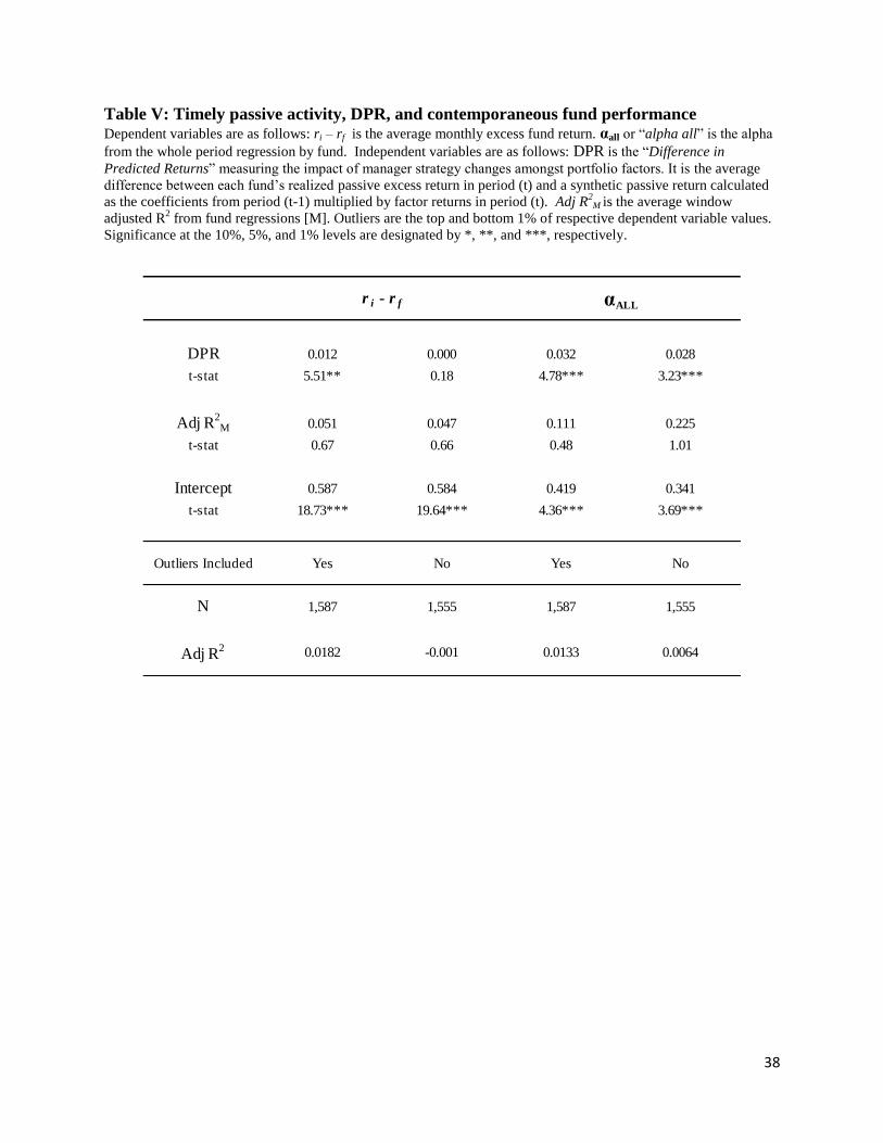
Our next test explores the relationship between timely strategy changes and fund

performance. DPR measures the degree to which managers’ strategy changes improve fund

returns compared to the “change nothing” strategy; if DPR is a positive determinant of fund

performance then at the mean, managers are able to anticipate economic changes and take

advantage of new opportunity sets, adding value net of transaction costs. Table 5 reports results

of our investigation.


Column two reports DPR is a positive determinant of excess returns, significant at the 5% level,

controlling for traditionally active management. We also find that DPR is positively and

statistically significantly (1% level) related to alpha. This strengthens our argument that although

short term alphas may be small or even negative for passively active managers the overall alpha

could be large and significant. Thus timely changes amongst passive portfolio strategies

contribute to investor returns, net of transaction costs and fees, and passively active managers are

adding relative value even when measured in terms of that typically reserved for active

managers.

SuPass measures the success with which managers’ passive portfolio bets are the most

profitable, that is, how well a manager contemporaneously chose to invest in the most profitable

factors.


Presumably, positive passive factor returns should be reflected in fund excess returns. Table 6

reports results of regressions of fund excess returns and alpha on SuPass, controlling for

traditionally active management. Results of the excess returns regressions are surprising.

23

Managers’ ability to correctly choose and capture the most profitable excess factor returns is

negative and significant, but this appears to be driven by outliers in column two. SuPass and

excess fund returns are positively related, as one would intuit, in column three but the coefficient

is insignificant. Not surprising, however, is the relationship between SuPass and fund alphas;

SuPass is negative and significant at better than the 1% level. Those managers who are most

effective at capturing passive portfolio excess returns are also those most likely to produce low

or negative alphas. Current terminology would potentially underrate these managers as

comparatively weak managers.

Our variables measure different aspects of passive activity. |Dα| measures the level of

activity, DPR measures relative performance as the efficacy of timely strategy changes compared

to no changes in strategy, and SuPass measures the extent to which managers correctly choose

profitable factor portfolios not once, but over time. In order to measure the relative impact of

passive variables on fund performance we rerun the regression to include all three measures of

passive activity on fund performance.


Table 7 reports results of these regressions. When we include all three measures of passivity in

regressions on concurrent realized excess returns we find that both |Dα| and DPR are positive and

highly significant. Thus, the level of activity and timely strategy changes are associated with

superior excess returns. As expected, all three variables are negative and highly significantly

related to overall alpha; the more passively active and the better passive managers capture factor

returns the lower the fund alpha, our proxy for traditional activity.

24

Overall, we conclude that our measures of passive activity capture both the activity and

performance of passive managers. Passively active managers positively impact excess returns

while negatively impacting alpha; these findings illustrate that though traditionally, passive

management is considered if not bad, then less desirable than alpha delivery, passive activity

contributes to excess returns. Investors may therefore benefit by investing in funds exhibiting

higher passively active metrics.

b. Do ex-ante metrics impact ex-post returns?

The previous regressions measured the relationship between contemporaneous fund

performance and manager activity variables. While interesting, there are two issues to consider.

Firstly, activity variables are ultimately constructed from fund excess returns; they are

endogenously determined by construction, and we cannot therefore reliably claim that activity

variables are determinants of fund performance. Secondly, from the investor’s perspective,

concurrent metrics are largely irrelevant. For example, just as past returns are not indicative of

future returns17

, a fund manager who has successfully chosen profitable factors over time

(SuPass) may fail to do so going forward. We want to test whether past passive activity metrics

are predictive of future fund performance; that is, we want to see if our variables are predictive

of returns that are not “contaminated” in that they also go into the construction of the passive

activity variables.

We therefore run a series of regressions in which the dependent variable is the average

monthly excess return in the current window on the average of independent variables from all

17

For example, the U.S. Financial Industry Regulatory Authority (FINRA) required disclosure statement for a retail

fund of hedge funds and commodity trading advisors states, in all caps, “Past performance is not indicative of future

results. Trading futures and options involves substantial risk of loss no matter who is managing your money and

such an investment is not suitable for everyone. Selling options involves unlimited risk of loss. Investors must read

and understand the current disclosure document before investing.”

25

previous windows. In other words, we test the relationship between all past passive activity

variables to date and future returns. For each variable, therefore, we have

2

,( ) ,( )( )i f w v i w n R i w n ir r V R [7]

where (ri - rf)w is the average monthly fund excess return in window w, and V is the average of

either |Dα|, DPR, or SuPass from all (n) window regressions prior to window w, and R2 is the

adjusted-R2 from the baseline model [M] regression. As before, adjusted-R

2 controls for

traditionally active management. For example, we want to measure the extent to which average

DPR in windows one and two are predictive of fund returns in window three, controlling for

traditional activity. We have enough observations to study windows one and two metrics on the

third window returns, 1-3 on the fourth window fund returns, and 1-4 on the fifth window fund

returns. It is important to note that we measure windows in event time, where the ‘event’ is the

25th

month of fund existence in the database, as opposed to calendar time. This means that our

results are not the result of calendar events which may or may not be adequately controlled by

time fixed-effects regressions. Our results are robust across macroeconomic regimes.


Our first test measures the extent to which past passive activity, |Dα|, is predictive of future

fund excess returns. Table 8 reports results. Managers who are more passively active are also

those more likely to post higher future excess fund returns. |Dα| is a positive determinant of

future returns for windows three and four at better than the 1% level. That is, managers who have

been more active in changing strategies in the past are more likely to provide investors with

higher realized returns, net of fees and transaction costs. Further, these effects are persistent, as

26

windows three and four given our methodology correspond with the 7th

-8th

and 9th

-10th

years of a

fund’s existence, respectively. While growing in significance from window three to four, |Dα|

fails to be a significant determinant of window five excess returns, however.

A similar pattern is found when we investigate the relationship between past timely passive

activity, DPR, and future returns.


Managers appear to be “on the ball” in correctly anticipating and profiting from changing passive

opportunity sets. DPR is a positive and significant determinant of fund excess returns.

Significance is better than the 1% level for windows three and four, waning to marginality in

window five. Thus, managers who are superior timely passive managers, relative to “change

nothing” or “do nothing” managers, are more likely to deliver superior future returns.

Overall superior market timing, as measured by SuPass, shows mixed predictive ability. As

discussed above, it is intuitive that managers whom are best able to capture the most profitable

factor returns in a given period are also those who are able to pass along superior fund returns to

their investors. If this is not the case, either transaction costs are eroding fund excess returns or,

perhaps worse, passively superior managers are terrible traditionally active managers; passive

gains are more than erased by traditionally active losses. Table 10 reports results of regressions

of past market timing performance against future excess fund returns.


SuPass is a positive and significant determinant of excess fund returns in window three. In fact,

the economic significance of absolute ‘factor capture’ performance is greater than |Dα| and DPR

27

combined. Interestingly, this is only the case in the 7th

-8th

years of fund life, however. SuPass is

positive but insignificant in predicting window four returns and negative and significant in

predicting window five returns.

Finally, we wish to include all of our activity variables in the predictive regressions. Table 11

reports results.


Our variables measure different aspects of passively active management. When we include all

average past passive activity variables in the regressions, we are able to better distinguish the

relationships between the variables. The level of activity, |Dα|, is a positive and significant

determinant of future returns. Interestingly, the significance of |Dα| increases from 5% to 1%

levels from window three to four before waning to insignificance in period five. DPR,

managerial ability to correctly access and profit from changing opportunity sets, is a positive and

significant determinant of future excess returns in all windows at better than the 1% level.

SuPass, however, is negative but insignificant in window three while negative and significant in

windows four and five. This would seem counterintuitive; a manager’s ability to capture higher

factor returns should be correlated with higher excess returns. However, since DPR already

measures the profitability of timely strategy changes rather than broadly capturing passive factor

returns, it is likely that SuPass is capturing luck rather than skill. The longer a fund is active the

less likely that it remains lucky in capturing passive strategy returns.

c. The effects of tenure

The above results illustrate passively active managerial actions over time. They raise an

interesting question, however. Why would activity as measured by |Dα| be significant in earlier

28

periods and less so in later periods? Even DPR’s significance wanes if considering t-stats. Are

funds becoming less active18

or less skilled? In an attempt to measure the effects of time more

precisely we create a variable Tenure which is simply the longevity of manager tenure in months.

Hedge funds are highly manager-centric; a manager typically starts a fund and when the manager

quits, the fund ceases to exist either because it is liquidated or acquired. We have data on fund

inception dates, manager identities, and manager start dates so we are able to precisely measure

manager tenure. There are funds that change managers, of course, and when this happens we

drop the fund from the remaining regressions. Thus, we investigate the effects of single-manager

tenure on excess returns and passively active variables. Since we study funds in event time

rather than calendar time, we can only see the effects of tenure when we include all windows into

a single regression. We therefore run regressions inclusive of all windows, for example, of

average |Dα| from windows two and three on excess returns in window four, of average |Dα| from

windows one through four on excess returns in window five, and so on, all in one regression.

Table 12 reports results of regressions of future excess returns on all past window average

activity variables.


For all model specifications, tenure is a positive determinant of fund returns in all windows,

significant at better than the 1% level. Columns two and three report that |Dα| and DPR remain

positive and statistically significant at the 1% level even given that the regression includes latter

periods. Column four reports that SuPass, on its own, is positive but insignificant with the

inclusion of tenure in the regression.

18

Here active is of course ‘passive activity’, as we control for the extent to which the fund is traditionally active.

29

The last column of Table 12 reports results of the final regression of future excess returns on

all past activity variables, inclusive of manager tenure. Importantly, |Dα| and DPR are nearly

identical in magnitude and significance when we include tenure in the regression; activity and

timely strategy changes are positive determinants of future excess returns. SuPass, while positive

and insignificant on its own is now negative and significant, at the 1% level, just as in Table 11.

Tenure is also a positive determinant of excess fund returns in future periods, significant at the

1% level. Experience counts. As to why passively active metrics erode in predictive power, or

worse, become negative determinants, over time, we have three explanations. The first is simply

survivorship bias. There are far more funds in existence in window three than in window five.

Those funds surviving through window five have been active, with one manager, for a minimum

of twelve years. Since the average life of all hedge funds is approximately five years, this is a

very long time. It may simply be that those funds with long lives are funds that are consistent,

excellent performers; there is not enough variation in the metrics of long lived passively active

funds. A second explanation is that passively active funds have shorter life-spans than

traditionally active funds, supporting the findings of Fung, Hsieh, Naik and Ramadorai (2008)

who find that “beta only”, or passive funds, have a liquidation rate of 22% in five years versus

7% for “have alpha”, or active funds. If so, it would seem to argue against the findings of

Aggarwal and Jorion (2010) that increased manager tenure decreases alpha, not excess returns.

Our third conjecture is that managers do indeed perform best in the earlier periods when possible

incentive and flow effects19

have the greatest impact on managerial desire to perform, and

therefore to exert effort. The most obvious conclusion is that all three effects could be at work.

19

Agarwal, Daniel and Naik (2009) find that funds with greater managerial incentives and discretion are associated

with positive fund performance; these effects are likely to be most pronounced in the earlier years of manager tenure

when managers are not as wealthy and additional investor flows have a significant impact on manager

compensation.

30

Experience counts, and the fact that measures of passive activity and performance decline over

time suggests that managers have less incentive (if not ability) to be active, traditionally or

passively, as personal wealth grows.

6. Conclusion

We create a methodology by which we identify traditionally active versus passively active

hedge fund management, where passively active managers choose amongst common hedge fund

industry strategies, or arbitrage portfolio factors. We identify the level of passive activity and the

relative and absolute performance of passively active managers. Alpha is the most commonly

used measurement of fund performance. It is also commonly used to identify superior

management skill, since alpha is that which is not, in theory, replicable by holding passive

portfolios. However, alpha is a measure of relative, not absolute performance. Further, it is

unlikely that even sophisticated investors would be able to passively hold hedge fund factor

portfolios, as these involve the replication of trend following, spreads, options, and futures

portfolios. Therefore it is desirable for investors to be able to measure managerial performance in

terms of excess returns, a measure of absolute, rather than purely relative, performance. It is also

desirable that investors in hedge funds be able to identify the type of manager activity, the degree

to which a manager is traditionally or passively active. Finally, investors would ideally like to

quantify not only the type and level of activity, but also the degree to which passively active

managers are able to correctly assess and profit from changing macroeconomic conditions and/or

choose profitable strategies.

Our methodology identifies the level of passive activity, |Dα| or “Absolute D Alpha”, the

degree to which managers correctly anticipate and react to changing conditions, DPR, or

“Difference in Predicted Returns”¸ and the success of passive activity in delivering excess

31

returns, SuPass, or “Superior Passive”. Traditionally active funds are not the only “good” funds;

passively active hedge funds also deliver superior excess returns. Our methodology identifies

managers who are likely to exhibit superior performance in the future.

32

References

Ackerman, Carl, Richard McEnally, and David Ravenscraft, 1999, The performance of hedge funds: risk,

return, and incentives, Journal of Finance 54, 3 833-874.

Agarwal, Vikas, Daniel, Naveen D., and Narayan Y. Naik, 2009, Role of managerial incentives and

discretion in hedge fund performance, Journal of Finance 64, 2221-56.

Agarwal, Vikas, and Narayan Y. Naik, 2000, Multi-period performance persistence analysis of hedge

funds, Journal of Financial and Quantitative Analysis 35, 327-42.

Agarwal, Vikas, and Narayan Y. Naik, 2004, Risk and portfolio decisions involving hedge funds, Review

of Financial Studies 17, 63-98.

Aggarwal, Rajesh K. and Philippe Jorion, 2010, The performance of emerging hedge funds and managers,

Journal of Financial Economics 96, 238-56.

Amihud, Yakov and Ruslan Goyenko, 2011, Mutual funds’ R2 as predictor of performance, Working

paper, New York University and McGill University.

Avramov, Doron, Kosowski, Robert, Naik, Narayan Y., and Melvyn Teo, 2011, Hedge funds, managerial

skill, and macroeconomic variables, Journal of Financial Economics 99, 672-92.

Baquero, Guillermo, Jenke ter Horst, and Marno Verbeek, 2005, Survival, look-ahead bias and the

persistence of hedge fund performance, Journal of Financial and Quantitative Analysis 40, 493-517.

Berk, Jonathan B., and Richard C. Green, 2004, Mutual fund flows and performance in rational markets,

Journal of Political Economy 112, 1269-95.

Cremers, K.J. Martijn and Antti Petajisto, 2009, How active is your fund manager? A new measure that

predicts performance, Review of Financial Studies 22, 3329-3365.

Fung, William and David A. Hsieh, 1999, A primer on hedge funds, Journal of Empirical Finance 6, 309-

31.

Fung, William and David A. Hsieh, 2000, Performance characteristics of hedge funds and commodity

funds: Natural vs. spurious biases, Journal of Financial and Quantitative Analysis 35, 291-307.

Fung, William and David A. Hsieh, 2001, The risk in hedge fund strategies: theory and evidence from

trend followers, Review of Financial Studies 14, 313-341.

Fung, William and David A. Hsieh, 2002, Hedge fund benchmarks: Information content and biases,

Financial Analysts Journal 58, 22-34.

Fung, William and David A. Hsieh, 2004, Hedge fund benchmarks: A risk-based approach, Financial

Analysts Journal 60, 65-80.

Fung, William, Hsieh, David A., Naik, Narayan Y., and Tarun Ramadorai, 2008, Hedge funds:

performance, risk, and capital formation, Journal of Finance 63, 1777-803.

Getmansky, Mila, Lo, Andrew W., and Igor Makarov, An econometric model of serial correlation and

illiquidity in hedge fund returns, Journal of Financial Economics 74, 529-609.

33

Jagannathan, Ravi, Alexey Malakhov, and Dmitry Novikov, 2010. Do hot hands exist among hedge fund

managers? An empirical evaluation, Journal of Finance 65, 217-255.

Kacperczyk, Marcin, Sialm, Clemens, and Lu Zheng, 2008, Unobserved actions of mutual funds, Review

of Financial Studies 21, 2379-2416.

Kosowski, Robert, Naik, Narayan Y., an d Melvyn Teo, 2007, Do hedge funds deliver alpha? A Bayesian

and bootstrap analysis, Journal of Financial Economics 84, 229-64.

Liang, Bing, 2000, Hedge funds: The living and the dead, Journal of Financial and Quantitative Analysis

35, 309-326.

Lo, Andrew W., 2008, A new measure of active management, Hedge Funds: An Analytic Perspective,

Princeton University Press, 168-196.

McCumber, William R., 2011, Seeking alpha, getting beta: a comparison of mutual and hedge fund

performance, style attribution, and active management fees, Working paper, University of Arkansas.

Mitchell, Mark and Todd Pulvino, 2001, Characteristics of risk and return in risk arbitrage, Journal of

Finance 56, 2135-75.

Sharpe, William F., 1992. Asset allocation: management style and performance management. Journal of

Portfolio Management, Winter 1992, 7-19.

Sun, Zheng, Wang, Ashley, and Lu Zheng, 2011, The road less traveled: strategy distinctiveness and

hedge fund performance, Working paper, University of California at Irvine.

34

Table I: Summary Statistics Summary statistics of all hedge funds 1994-2010.

Active Funds as of December 31, 2010 (1,565 funds) Obs Mean Median Std Dev Min Max

monthly excess return 180,330 0.77 0.64 5.75 -90.27 344.01

management fee 1,565 1.46 1.50 0.67 0.00 6.00

performance fee 1,565 17.62 20.00 6.60 0.00 50.00

high-water mark 1,565 0.88 1.00 0.32 0.00 1.00

total assets 182,759 309 61 2,210 0 96,458

longevity, in months 1,565 130 121 42 10 205

funds self-identified as Obs Mean Obs Mean

long-short equity 487 0.311 42 0.027

managed futures 225 0.144 27 0.017

multi-style 163 0.104 33 0.021

macro 124 0.079 27 0.017

equity fundamental 92 0.059 11 0.007

long bias equity 99 0.063 23 0.015

undisclosed style 0 0 19 0.012

distressed securities 66 0.042 6 0.004

emerging market equity 74 0.047 3 0.002

fixed income arbitrage 49 0.031

Inactive Funds as of December 31, 2010 (3,385 funds) Obs Mean Median Std Dev Min Max


management fee 3,385 1.50 1.50 0.72 0.00 6.00

performance fee 3,385 17.51 20.00 6.50 0.00 50.00

high-water mark 3,385 0.75 1.00 0.44 0.00 1.00

total assets 198,087 197 20 1,945 0 72,040


funds that were

acquired 114 0.03

liquidated 1,607 0.47




multi-style 359 0.106 74 0.022

macro 294 0.087 51 0.015



undisclosed style 288 0.085 27 0.008




convertible arbitrage

asset backed securities

short biased equity


fixed income

mortgage-backed arbitrage

capital structure arbitrage

equity statistical arbitrage

emerging markets debt

merger arbitrage

fixed income


merger arbitrage





short biased equity

35

Table II: Summary Statistics, 96’ers Summary statistics of 1,587 hedge funds with sufficient longevity to calculate performance metrics and 3,363 funds

without sufficient monthly observations. 96’ers are funds with at least 96 monthly observations; the first 24 months

are discarded to correct for backfill bias and remaining months are divided into non-overlapping 24 month windows

of observation.

96'ers (1,587 funds) Obs Mean Median Std Dev Min Max


management fee 1,587 1.49 1.50 0.76 0.00 6.00

performance fee 1,587 17.71 20.00 6.47 0.00 50.00

high-water mark 1,587 0.86 1.00 0.35 0.00 1.00

total assets 210,948 271 45 1,869 0 72,040


funds that were

acquired 18 0.01

liquidated 234 0.15




multi-style 162 0.102 41 0.026

macro 140 0.088 27 0.017







non-96'ers (3,363 funds) Obs Mean Median Std Dev Min Max


management fee 3,363 1.48 1.50 0.62 0.00 6.00

performance fee 3,363 17.37 20.00 6.65 0.00 50.00

high-water mark 3,363 0.75 1.00 0.43 0.00 1.00

total assets 169,898 227 25 2,309 0 96,458


funds that were

acquired 84 0.03

liquidated 1,247 0.37




multi-style 367 0.109 54 0.016

macro 256 0.076 47 0.014








short biased equity






fixed income

merger arbitrage






fixed income

merger arbitrage

short biased equity


36

Table III: Summary statistics of traditionally and passively active management metrics Adj R

2M is the average window adjusted R

2 from fund regressions [M], a proxy for traditionally active management.

|Dα| or “absolute D alpha” is the absolute value of the difference between αall and the average of fund window (non-

overlapping 24- month) regressions, where αall or “alpha all” is the alpha from the whole period regression. DPR or

“Difference in Predicted Returns” is the average difference between each fund’s realized passive excess return in

period (t) and a synthetic return. The synthetic return is calculated as the coefficients from period (t-1) multiplied by

factor returns in period (t). SuPass or “Superior Passive” is the average percentage of maximum possible factor

returns captured by fund managers over regression windows. The latter three variables are fund averages of

measurements of passively active management. Outliers are the top and bottom 1% of all observations of each

variable.

Obs Mean Median Std Dev Min Max

Adj R2M 1,555 0.356 0.353 0.201 -0.092 0.819

|Dα| 1,555 2.908 1.873 3.051 0.025 18.488

DPR 1,555 0.262 -0.021 5.550 -18.044 25.533

SuPass 1,555 0.469 0.481 0.577 -2.331 2.735

Obs Mean Median Std Dev Min Max

Adj R2M 1,587 0.356 0.353 0.212 -0.234 0.958

|Dα| 1,587 3.142 1.873 4.134 0.002 48.870

DPR 1,587 0.321 -0.021 7.279 -51.062 60.365

SuPass 1,587 0.455 0.481 0.780 -7.847 4.847

outliers excluded

outliers included

37

Table IV: Level of passive activity, |Dα|, and contemporaneous fund performance Dependent variables are as follows: ri – rf is the average monthly excess fund return. αall or “alpha all” is the alpha

from the whole period regression by fund. Independent variables are as follows: |Dα| or “absolute D alpha” is a

measure of absolute passive activity; it is the absolute value of the difference between αall and the average of fund

window (non-overlapping 24- month) regressions. Adj R2M is the average window adjusted R

2 from fund regressions

[M]. Outliers are the top and bottom 1% of respective dependent variable values. Significance at the 10%, 5%, and

1% levels are designated by *, **, and ***, respectively.

|Dα| 0.033 0.032 0.046 0.035

t-stat 6.77*** 7.57*** 3.08*** 2.85***

Adj R2M 0.059 -0.008 0.156 0.288

t-stat 0.78 -0.12 0.67 1.53

Intercept 0.492 0.512 0.278 0.258

t-stat 14.05*** 18.02*** 2.65*** 3.05***

NoYes

r i - r f αALL

Outliers Included

Adj R2 0.0275 0.0344 0.0051 0.0056

1,5551,5871,5551,587N

NoYes

38

Table V: Timely passive activity, DPR, and contemporaneous fund performance Dependent variables are as follows: ri – rf is the average monthly excess fund return. αall or “alpha all” is the alpha

from the whole period regression by fund. Independent variables are as follows: DPR is the “Difference in

Predicted Returns” measuring the impact of manager strategy changes amongst portfolio factors. It is the average

difference between each fund’s realized passive excess return in period (t) and a synthetic passive return calculated

as the coefficients from period (t-1) multiplied by factor returns in period (t). Adj R2

M is the average window

adjusted R2 from fund regressions [M]. Outliers are the top and bottom 1% of respective dependent variable values.

Significance at the 10%, 5%, and 1% levels are designated by *, **, and ***, respectively.

DPR 0.012 0.000 0.032 0.028

t-stat 5.51** 0.18 4.78*** 3.23***

Adj R2M 0.051 0.047 0.111 0.225

t-stat 0.67 0.66 0.48 1.01

Intercept 0.587 0.584 0.419 0.341

t-stat 18.73*** 19.64*** 4.36*** 3.69***

NoYesNoYesOutliers Included

1,5551,5871,5551,587N

0.00640.0133-0.0010.0182Adj R2

r i - r f αALL

39

Table VI: Factor capture, SuPass, and contemporaneous fund performance Dependent variables are as follows: ri – rf is the average monthly excess fund return. αall or “alpha all” is the alpha

from the whole period regression by fund. Independent variables are as follows SuPass or “Superior Passive” is a

measure of managerial success in capturing profitable factor returns. It is the average percentage of maximum

possible factor returns captured by fund managers over regression windows. Adj R2M is the average window adjusted

R2 from fund regressions [M]. Outliers are the top and bottom 1% of respective dependent variable values.


SuPass -0.051 0.021 -1.252 -1.649

t-stat -2.47** 0.76 -22.62*** -23.11***

Adj R2M 0.064 0.045 -0.166 -0.189

t-stat 0.83 0.60 -0.82 -0.98

Intercept 0.610 0.573 1.098 1.316

t-stat 18.16*** 16.89*** 12.26*** 14.87***

NoYesOutliers Included

0.2436

1,587

0.3287

1,555

NoYes

Adj R2

N

0.0032

1,587

-0.0007

1,555

r i - r f αALL

40

Table VII: Passive activity metrics and contemporaneous fund performance Dependent variables are as follows: ri – rf is the average monthly excess fund return. αall or “alpha all” is the alpha

from the whole period regression by fund. Independent variables are as follows: |Dα| or “absolute D alpha” is the

absolute value of the difference between αall and the average of fund window (non-overlapping 24- month)

regressions. DPR or “Difference in Predicted Returns” is the average difference between each fund’s realized

passive excess return in period (t) and a synthetic return. The synthetic return is calculated as the coefficients from

period (t-1) multiplied by factor returns in period (t). SuPass or “Superior Passive” is the average percentage of

maximum possible factor returns captured by fund managers over regression windows. Adj R2

M is the average

window adjusted R2 from fund regressions [M]. Significance at the 10%, 5%, and 1% levels are designated by *, **,

and ***, respectively.

|Dα| 0.030 0.032 -0.044 -0.027

t-stat 5.93*** 7.26*** -3.26*** -2.30**

DPR 0.011 0.004 -0.041 -0.040

t-stat 4.44*** 1.93* -6.16*** -6.93***

SuPass 0.039 0.026 -1.498 -1.121

t-stat 1.64 1.18 -23.33*** -19.53***

Adj R2M 0.047 -0.007 -0.118 0.077

t-stat 0.62 -0.11 -0.59 0.46

Intercept 0.482 0.500 1.336 1.032

t-stat 12.84*** 15.75*** 13.31*** 12.06***

0.2026

1,555

NoYes

Adj R2

N

0.0384

1,587

0.0356

1,555

NoYesOutliers Included

0.2669

1,587

r i - r f αALL

41

Table VIII: Ex-ante passive activity, |Dα|, and ex-post fund performance The dependent variable in all cases is the average of monthly excess returns, (ri – rf), for the next non-overlapping

24 month window. Independent variables are as follows: |Dα| or “absolute D alpha” is the absolute value of the

difference between αall and the average of fund window (non-overlapping 24- month) regressions, where αall or

“alpha all” is the alpha from the whole period regression by fund. Adj R2

M is the average window adjusted R2 from

fund regressions [M]. |Dα| and Adj R2 are averages of previous window regressions. Significance at the 10%, 5%,

and 1% levels are designated by *, **, and ***, respectively.

|Dα| 0.02383 0.05344 0.01383

t-stat 3.79*** 6.05*** 1.04

Adj R2

M -0.04071 0.1617 0.32711

t-stat -0.27 0.82 1.23

Intercept 0.32967 0.28493 0.2809

t-stat 5.20*** 3.35*** 2.39**

Adj R2

N

0.0013

531

0.0374

923

0.0078

1,587

2 predicting 3 3 predicting 4 4 predicting 5

42

Table IX: Ex-ante timely activity, DPR, and ex-post fund performance The dependent variable in all cases is the average of monthly excess returns, (ri – rf), for the next non-overlapping

24 month window. Independent variables are as follows: DPR or “Difference in Predicted Returns” is the average

difference between each fund’s realized passive excess return in period (t) and a synthetic return. The synthetic

return is calculated as the coefficients from period (t-1) multiplied by factor returns in period (t). Adj R2M is the

average window adjusted R2 from fund regressions [M]. DPR and Adj R

2M are averages of previous window

regressions. Significance at the 10%, 5%, and 1% levels are designated by *, **, and ***, respectively.

DPR 0.01747 0.01325 0.00642

t-stat 9.97*** 4.78*** 1.68*

Adj R2

M -0.11345 0.2096 0.26493

t-stat -0.77 1.06 1.16

Intercept 0.4852 0.46875 0.32627

t-stat 8.19*** 5.89*** 2.99***

Adj R2

N

0.0046

531

0.0234

923

0.0579

1,587


43

Table X: Ex-ante factor capture, SuPass, and ex-post fund performance The dependent variable in all cases is the average of monthly excess returns, (ri – rf), for the next non-overlapping

24 month window. Independent variables are as follows: SuPass or “Superior Passive” is the average percentage of

maximum possible factor returns captured by fund managers over regression windows. Adj R2M is the average

window adjusted R2 from fund regressions [M]. SuPass and Adj R

2M are averages of previous window regressions.


SuPass 0.07145 0.01821 -0.14041

t-stat 2.99*** 1.11 -2.43**

Adj R2

M -0.01482 0.2233 0.32581

t-stat 0.92 0.27 0.22

Intercept 0.41138 0.46504 0.40648

t-stat 11.23*** 11.68*** 3.57***

0.0104

531

-0.0005

923

0.0043

1,587

Adj R2

N


44

Table XI: Ex-ante active management metrics and ex-post fund performance The dependent variable in all cases is the average of monthly excess returns, (ri – rf), for the next non-overlapping



“alpha all” is the alpha from the whole period regression by fund. DPR or “Difference in Predicted Returns” is

the average difference between each fund’s realized passive excess return in period (t) and a synthetic return. The

synthetic return is calculated as the coefficients from period (t-1) multiplied by factor returns in period (t). SuPass or

“Superior Passive” is the average percentage of maximum possible factor returns captured by fund managers over

regression windows. Adj R2

M is the average window adjusted R2 from fund regressions [M]. Significance at the

10%, 5%, and 1% levels are designated by *, **, and ***, respectively.

|Dα| 0.015 0.048 0.020

t-stat 2.28** 5.44*** 1.50

DPR 0.017 0.016 0.013

t-stat 8.78*** 5.81*** 3.11***

SuPass -0.013 -0.108 -0.220

t-stat -0.5 -2.74*** -3.51***

Adj R2

M-0.125 0.139 0.240

t-stat -0.86 0.71 0.91

Intercept 0.431 0.360 0.391

t-stat 6.39*** 4.13*** 3.24***

0.0266

531

0.0591

923

0.0605

1,587

Adj R2

N


45

Table XII: The effects of manager tenure The dependent variable in all cases is the average of monthly excess returns, (ri – rf), for the next non-overlapping



“alpha all” is the alpha from the whole period regression by fund. DPR or “Difference in Predicted Returns” is the

average difference between each fund’s realized passive excess return in period (t) and a synthetic return. The

synthetic return is calculated as the coefficients from period (t-1) multiplied by factor returns in period (t). SuPass or

“Superior Passive” is the average percentage of maximum possible factor returns captured by fund managers over

regression windows. |Dα|, SPR, and SuPass metrics are averages of these variables over all previous regression

windows. Adj R2

M is the average window adjusted R2 from all previous fund window regressions [M]. Tenure is

manager tenure, in months. Significance at the 10%, 5%, and 1% levels are designated by *, **, and ***,

respectively.

|Dα| 0.031 0.024

t-stat 5.51*** 4.28***

DPR 0.015 0.017

t-stat 9.39*** 9.12***

SuPass 0.032 -0.066

t-stat 1.43 -2.70***

Adj R2M 0.083 0.047 0.113 0.019

t-stat 0.62 0.35 0.83 0.15

Tenure 0.329 0.395 0.400 0.337

t-stat 3.49*** 4.28*** 4.23*** 3.64***

Intercept -0.034 0.027 -0.014 0.039

t-stat -0.27 0.22 -0.11 0.31

0.0224

2,011

Adj R2

N

0.0616

2,011

0.0087

2,011

0.0494

2,011

Model 4Model 1 Model 2 Model 3

how active could passive hedge fund management be?

Documents