CDE November 2014

How Backward are the Other Backward Classes? Changing Contours of Caste

Disadvantage in India

Ashwini Deshpande Email:ashwini@econdse.org Department of Economics Delhi School of Economics

Rajesh Ramachandran Email: ramachandranrajesh6@gmail.com

Department of Microeconomics and Management Goethe University, Frankfurt

Working Paper No. 233 (Revised)

Centre for Development Economics Department of Economics, Delhi School of Economics

How Backward are the Other Backward Classes? Changing

Contours of Caste Disadvantage in India

Ashwini Deshpande and Rajesh Ramachandran∗

November 2014

Abstract

We trace changes in standard-of-living indicators across the three broad caste groups in India in order

to comment on the evolution of the relative ranking of “Other Backward Classes” (OBCs). Employing a

difference-in-differences strategy and analyzing individuals born between 1926-1985, we find convergence

in primary and secondary education, but continued divergence in higher education. Younger cohorts of

OBCs converge with upper castes in wages and white-collar jobs. The extension of affirmative action

increases the share of OBCs with government jobs and secondary education, though increased political

representation does not seem to be correlated with better outcomes.

1 Introduction

The rise of the Other Backward Classes (OBCs) in the political arena since the mid-1980s has been heralded

as India’s “silent revolution” (Jaffrelot, 2003). This political ascendancy has also been viewed as representing

a large enough flux in the traditional hierarchies of the caste system, such that we now have “a plethora

of assertive caste identities... [that] articulate alternative hierarchies” leading to a scenario where “there is

hardly any unanimity on ranking between jatis” (Gupta, 2009). Indeed, there is no doubt, especially since

the 73rd and 74th constitutional amendments in the early 1990s, that the so-called lower castes have become

an important force in Indian politics at all levels - local, state and national. Has this change in the political

arena been accompanied by a corresponding reshuffling of the traditional economic hierarchies, such as to

∗Deshpande: Delhi School of Economics, University of Delhi, ashwini@econdse.org. Ramachandran: Department of Microe-conomics and Management, Goethe University, Frankfurt, ramachandran@econ.uni-frankfurt.de.We would like to thank Alessandro Tarozzi, Ana-Rute Cardoso and Irma Clots Figueras for their suggestions and comments.We are also grateful to conference participants at Yale University, Indian Statistical Institute, New Delhi, and at the WorldBank-International Economic Association roundtable on Inequality, Jordan, where earlier versions of this paper were presented,for their suggestions and useful comments. We are responsible for all remaining errors and omissions.

1

prevent any meaningful ranking of castes?1

The nature and degree of change in the economic ranking between castes, or broad caste groups, is a

matter of empirical verification. While there is a large and growing body of work documenting the changes in

the standard of living indicators of the Scheduled Castes and Tribes (SCs and STs), as well as the economic

discrimination faced by these groups, (see Deshpande 2011, for a review of the recent research), the discussion

about the material conditions or the economic dominance of the group of castes and communities classified

as the “Other Backward Classes” (OBCs) in India is prompted more by beliefs, or localized case studies,

rather than by an empirical analysis of the macro evidence. Part of the reason for this lacuna is the lack of

hard data: until the 2001 census, OBCs were not counted as a separate category, while affirmative action

(quotas in India) was targeted towards OBCs at the national level since 1991, and at the state level since

much earlier. This would be the only instance of an affirmative action program in the world, where the

targeted beneficiaries are not counted as a separate category in the country’s census.

Researchers have, therefore, had to rely on data from large sample surveys, such as the National Sample

Survey (NSS) or the National Family and Health Survey (NFHS), in order to get estimates about the material

conditions of the OBCs. The use of this data has generated research which undertakes a broader analysis of

various caste groups, OBCs being one of the groups in the analysis, along with the SC- STs and “Others”, the

residual group comprising the non-SC-ST-OBC population (for instance, Deshpande 2007; Iyer et al. 2013;

Madheswaran and Attewell 2007; Zacharias and Vakulabharanam 2011, among others). “Others” include

the Hindu upper castes and could be considered a loose approximation for the latter, but data constraints

do not allow us to isolate the upper castes exclusively. Existing evidence suggests that OBCs lie somewhere

in between the SC-STs and the Others, but first, very little is known about their relative distance from

the two other categories, and second, in order to make a meaningful intervention about the possible links

between their political ascendancy and their economic conditions, it is important to trace how their relative

economic position has changed vis-a -vis the other two groups over time. Here again, the economic researcher

is stymied by the lack of good longitudinal data.

The present paper is an attempt to fill this caveat in the empirical literature by focusing on an important

facet of contemporary caste inequalities, viz., the changing economic conditions of OBCs, relative to the other

two broad social/caste groups. We use data from two quinquennial rounds of the employment-unemployment

surveys (EUS) of the NSS for 1999-2000 and 2009-10 (NSS-55 and NSS-66, respectively), to examine the

multiple dimensions of material standard of living indicators, and the changes therein for the OBCs in India,

1The caste system is a system of graded inequalities, with the so-called upper castes conventionally at the top of the socio-economic hierarchy, and the ex-untouchable castes, now clubbed together in the official category of Scheduled Castes are at thebottom. For details about the caste system, see Deshpande (2011).

2

in comparison to SC-STs and the Others.2 We construct six cohorts aged between 25 and 84 years in 2010

from the two NSS rounds, and examine changes in multiple indicators using a difference-in-differences (D-I-

D) approach, comparing the three social groups to one another to see how the gaps on the key indicators of

interest have evolved over the 60-year period. This allows us to gauge the relative generational shifts between

the major caste groups. Our analysis focuses particularly on the OBCs, and compares how the evolution

of the different OBC cohorts (in relation to the Others) compares with the evolution of the corresponding

SC-ST cohorts to the Others.

Through an analysis based on a comparison of different age cohorts, we are able to build a comprehensive

trajectory of change for each of the caste groups since independence, since the oldest cohort in our analysis

consists of individuals born between 1926 and 1935, and the youngest cohort consists of those born between

1976 and 1985. Thus, we are able to track outcomes for successive generations of individuals who reached

adulthood in the 63 years between Indian independence (in 1947) and 2010.

Our main results can be summarized as follows. In a three-fold division of the population between SC-

STs, OBCs and Others, we see clear disparities in virtually all indicators of material wellbeing marginal per

capita consumption expenditure (MPCE), years of education, wages, occupational categories - with Others

at the top, SC-STs at the bottom and OBCs in between, and indicates that there is no absolute reversal of

traditional caste hierarchies.

Looking at patterns of convergence/divergence and comparing the cohort born during 1926-35 to the one

born during 1976-85, for the OBCs and Others, we find that OBCs fall further behind in accumulation of

human capital as captured by the years of education. Breaking down the composite indicator of “years of

education”, we find evidence of convergence between OBCs and Others in literacy and primary education,

but continued divergence when higher educational categories are considered.

In the realm of occupation, comparison of cohorts born during 1976-85 to the one born during 1936-45

shows that the OBCs fall further behind the Others in access to white-collar jobs by 2.7 percentage points.

For the category of regular wage/salaried (RWS) jobs, we find divergence between the Others and the other

two social groups: OBCs and SC-STs. The OBC cohort born during 1966-75 has nearly one-third of the

individuals still involved in “casual jobs”. This proportion has increased for all three social groups, which

indicates that economic growth over the period has not created secure formal sector jobs for a large majority

of the population.

Looking at average wage gaps for males in RWS occupations, we find that while average wages of Others

2For the purpose of this paper, we have pooled the two groups of SCs and STs, because despite considerable differencesin their social situation, their economic outcomes are very similar. In between these two rounds NSS also conducted anotherquinquennial survey in 2004-05, NSS-61. We believe a decade is a good length of time to compare trends, therefore we focuson two rounds which are 10-years apart.

3

are higher than those for OBCs for all age cohorts, though the gap reduces for cohorts born after 1955.

However the “unexplained” component is lower for the cohort aged 35-44 in 2010, as compared to those aged

45-54 or 25-34 in 2010. The absolute gaps in average daily wages between Others and SC-STs are higher

than those between Others and OBCs, but decompositions reveal that the unexplained part is greater for

OBCs than for SC-STs.

An important corollary of the political rise of the OBCs has been the extension of quotas at the central

level by a further 27 percent for OBCs, in addition to the quotas for SC-STs. We specifically examine if the

extension of affirmative action to OBCs had any significant impact on their occupational and educational

attainment. Identification of a causal impact of the 1991 policy change is complicated due to the already

existing and ever-changing quotas at the state level. Our identification strategy exploits the differential

impact the policy had depending on the age and caste group of the individual. In support of our identifying

assumption, we first show that the OBCs exhibit identical trends with respect to the SC-ST and Others in

access to public sector jobs and completion of secondary education prior to the policy change. The effect of

the 1991 policy can be seen in our main estimation results which show that affirmative action increased the

percentage of OBCs obtaining public sector jobs and finishing secondary education by 2.6 and 4 percentage

points, respectively.

Finally we explore whether increase in political representation of OBCs in state assemblies after 1991

could be correlated with their changed outcomes, especially reflected in indicators such as likelihood of being

a graduate or access to white collar jobs. We use the typology outlined in Jaffrelot (2003), which groups

Indian states into seven types depending on the evolution of the share of OBC members of legislative assembly

(MLAs) in the various states. Our preliminary analysis shows that the OBCs not only perform the worst

in the states of Uttar Pradesh, Bihar, Madhya Pradesh, Punjab, Rajasthan and Gujarat, the states where

political representation increases the most, but also lose ground to the Others over the period analyzed, and

hence find little support for the “silent revolution” having had a significant impact on economic outcomes.

The rest of the paper is organized as follows: Section 2 provides some background on who the OBCs are;

Section 3 analyses evolution on household level indicators; Section 4 deals with trends in education; Section 5

discusses trends in occupation; Section 6 examines wages and presents estimates of the share of wages not

explained by observable characteristics; Section 7 explores the role of affirmative action in explaining the rise

in education attainment; Section 8 preliminarily investigates the link, if any, between political representation

and socio-economic outcomes of OBCs; and Section 8 concludes.

4

2 Who are the OBCs?

Parts of British India enacted preferential policies for the “Depressed Classes”, which included communities

that were classified as “backward”, as well as for the untouchables, tribals and some non-Hindu communities.

Even though there were preferential policies for the “Backward Classes”, their exact definition had not

been clearly articulated and details of the various definitions employed during the British period are spelt

out in Galanter (1984). The constitution of independent India did not define Other Backward Classes

(OBCs) in a specific way either. However, after the Scheduled Castes were listed as a separate category,

the term Backward Classes started to be used in two senses: one, as the group of all communities that

needed preferential treatment, and two, as castes low in the socio-economic hierarchy, but not as low as the

untouchables. We should note that the two usages overlap considerably. However, the exact identification

of groups and communities to be counted as OBCs has been fraught with a great deal of controversy.

Even before the constitution of independent India came into effect in 1950, several states formed the

category of OBCs for the first time (e.g. Bihar in 1947; Uttar Pradesh in 1948) and conferred benefits

on them, while those states which already had benefits for the backward castes from before independence,

expanded the existing range of benefits. Thus, in 1978, without any central reservations for OBCs, at least

13 states reserved seats for Backward Classes, other than SCs and STs. These reservations were found

throughout southern India, in Maharashtra and Gujarat and in parts of north India, with the heaviest

representation in the south (Galanter 1984, 87).

The first Backward Classes Commission (with Kaka Kalelkar as its chairman) was established in 1953,

which was directed to first ascertain the criteria that should be adopted to determine whether any section

of the population could be considered backward (other than the SC and ST), and then according to these

criteria, prepare a list of such classes. The Commission prepared a list of 2399 groups, which were roughly 32

per cent of the population. It was generally understood that the groups identified by the commission would

be castes or communities. This meant that backwardness was defined or understood in terms of the “social

hierarchy based on caste”. Thus, the commission listed as criteria of backwardness - trade and occupation,

security of employment, educational attainment, representation in government service and position in the

social hierarchy.

Much like the contemporary experience, there was a rush among communities wanting to be classified

as backward due to the potential benefits that this status would confer upon them. However, in deciding

on the validity of these multiple claims, the commission was stymied by the lack of data. Despite the lack

of data, the commission made wide-ranging recommendations for benefits to be conferred to the backward

classes, often relying on just the names of the caste to make its case. However, at the last minute, the

5

chairman repudiated the report of the commission by stating that he found the use of caste as antithetical to

democracy and to the eventual creation of a casteless and classless society. Due to several factors (the rush of

communities wanting to be classified as backward, the unreliability of data, the extensive recommendations

of the commission), the work of the commission was widely criticised. The basic point of contention was the

use of caste or community as one of the principal criteria to determine backwardness. There was a forceful

plea made to use economic criteria alone to determine backwardness, and hence decide which individuals

should be considered backward on the basis of objective economic indicators, rather than social criteria such

as castes or communities. In 1965, when the report was finally tabled in parliament, the central government

firmly opposed the definition of backwardness on the basis of communal criteria (i.e. communities or castes),

arguing that the use of caste was administratively unworkable and was contrary to the “first principles of

social justice” in their exclusion of other poor. The centre decided not to impose a uniform criterion on

the states, but persuaded them to use economic criteria, rather than community based ones, to identify the

backward.

Various state governments set up backward classes commissions, and some followed the economic criteria

endorsed by the Centre. However, most states continued to place a greater emphasis on the caste criterion.

The second Backward Classes commission was set up in 1978 under the chairmanship of B.P. Mandal to

examine the entire issue of backwardness, starting again with ascertaining the criteria that should be used

to identify the backward.

The Mandal Commission used 11 criteria to determine eligibility, which were grouped under three heads:

social, educational and economic. These were combined using weights (social criteria were given a weight

of three, educational got two and economic criteria were given a weight of one). This was done for all the

Hindu communities. For the non-Hindus, the commission used another set of criteria: all untouchables who

had converted to other religions but were still identifiable by their traditional occupations, for which the

Hindu counterparts were included in the list of backward classes, also got enlisted.

Based on this, the commission identified 3743 caste groups as backward, which were 52 per cent of the

population (as against 32 per cent identified by the Kalelkar commission and the roughly identified 40 per

cent from the NSS data). The 52 per cent figure was arrived at after subtracting from 100 per cent the

share of the SC-ST population, the non-Hindu population based on the 1971 census, and the share of the

Hindu upper castes extrapolated from the 1931 census. The residual was actually 43.7, to which was added

half of the non-Hindu population share. Since the identification of OBCs is done at the state-level, there

are communities identified as OBCs in one state, but not in another, e.g. Jats are classified as OBCs in

Rajasthan, but not in Haryana. Several of the communities classified as OBCs are “occupation castes” e.g.

darzi (tailor), teli (oil presser), julaha (weaver), sonar (goldsmith), kanbi (agricultural caste), madari (juggler

6

and/or monkey-minder, someone who earns money by showing tricks to a crowd), rangrez (painter), halwai

(sweetmeats and snacks maker) etc.

It is clear that seen at the national level, the OBC category is an omnibus one, which includes a diverse

set of communities. In some states, groups classified as OBCs are dominant landowning castes, such as

Kammas and Reddys in Andhra Pradesh, or Vokkaligas and Lingayats in Karnataka. These groups are not

necessarily backward in terms of their socio-economic status, but are included in the legal OBC category.

Our estimates cannot distinguish between dominant OBC castes and those that are truly backward, as the

OBC count with NSS data includes all the legal OBCs. We should note that in states where (legal) OBCs

are also dominant (in terms of status), the aggregate outcomes of OBCs would be pulled up, as the dominant

OBCs are also the landowning castes. This heterogeneity also characterizes the comparison social category of

“Others’ (and to a smaller extent, SCs and STs), such that the inclusion of poorer Others pulls the averages

for the Others category down. As a result, a comparison between these omnibus categories would understate

the actual gap between the top end of the “Others’, and those who are genuinely backward among the OBCs.

While the use of these broad categories limits a nuanced understanding of inter-community differences

within the category, the advantage is that it enables us to identify the “macro” picture, which smaller, case-

study-based comparisons do not allow, especially given that the number of communities runs into thousands.

3 The broad picture: household-level indicators

Table 1 presents estimates of four indicators of standard of living for the three major social groups: SC-STs

considered together, OBCs and the Others, for the two survey rounds, NSS-55 and NSS-66, respectively. The

indicators of interest are monthly per capita expenditure (MPCE), proportion of the group that is urban

(per cent urban) and two land holding measures: land owned and land possessed.

D-I-D for household-level variables is calculated as:

D − I −Djk = [(Indicatorijs − Indicatoriks) − (Indicatorij(s−1)) − Indicatorik(s−1))] (1)

where j and k are the two caste groups being compared, for the ith indicator (say MPCE) between survey

rounds s and s− 1.

MPCE is shown in nominal terms: Others have the highest MPCE, followed by OBCs, and then the

SC-STs. While the MPCE for each of the groups has expectedly increased in nominal terms, the D-I-D

allows us to see the relative gains of groups. In 1999-00 the gap between Others and OBCs was Rs. 167,

which increases to Rs. 462 in 2009-10. Thus for the OBCs, MPCE has fallen behind that of the Others by

Rs. 295 over the decade. A comparison of Others with SC-STs shows that the gap increases from Rs. 234 to

7

Rs. 639 over the two decades, implying that Others’ MPCE has increased by Rs. 405 relative to SC-STs over

the ten year period. Thus, SC-STs not only continue to have the lowest MPCE, but the other two groups

have gained relative to them in terms of MPCE. OBCs have gained relative to SC-STs, but the magnitude of

their falling behind Others is over 2.5 times their gain over SC-STs. Thus, on MPCE, there is no evidence of

convergence between Others and OBCs (or SC-STs). Urbanization (percent of the group’s population which

is urban) is an indicator of potential integration into the modern or formal sector economy. We see a rise in

urban proportions for both OBCs and Others (from 22 and 35 to 26 and 40 per cent, respectively between

the two survey rounds, but virtually no change for the SC-ST population at around 16 per cent in the same

time period). Again, looking at relative changes across groups using D-I-D, we find a similar pattern to the

indicator MPCE, with no evidence of convergence.

[Insert Table 1]

The two land holding variables (land possessed and land owned) show sharp disparities across caste groups in

both rounds, with average values for SC-STs slightly over half of the values for Others. However, in terms of

the relative change in these two variables, we see that OBCs marginally fell behind SC-STs by 0.02 hectares

for land possessed, but gained over Others by close to 0.07 hectares.3 SC-STs appear to have gained over

Others in both land owned and land possessed by 0.08 and 0.09 hectares respectively. These changes are

negligible in magnitude to have any real consequences for standard of living, and are clearly not matched by

the trends in MPCE.

Overall, at the household level, we see a clear hierarchy in MPCE, such that Others are at the top,

followed by OBCs and then SC-STs. Over the decade, the gap between OBCs and SC-STs has increased in

favor of the former, and Others’ MPCE has increased relative to both SC-STs and OBCs, but the magnitude

of gain has been larger vis-a -vis the SC-STs than OBCs.

4 Individual-level characteristics: Education

In order to analyze the trends over time in the relative position of the three social groups, we construct six

birth cohorts using the age variable in each of the NSS rounds as shown in Table 2.

[Insert Table 2]

31 acre=0.4047 hectares. Land possessed is defined as land (owned+leased-in+neither owned nor leased- in) - land leasedout.

8

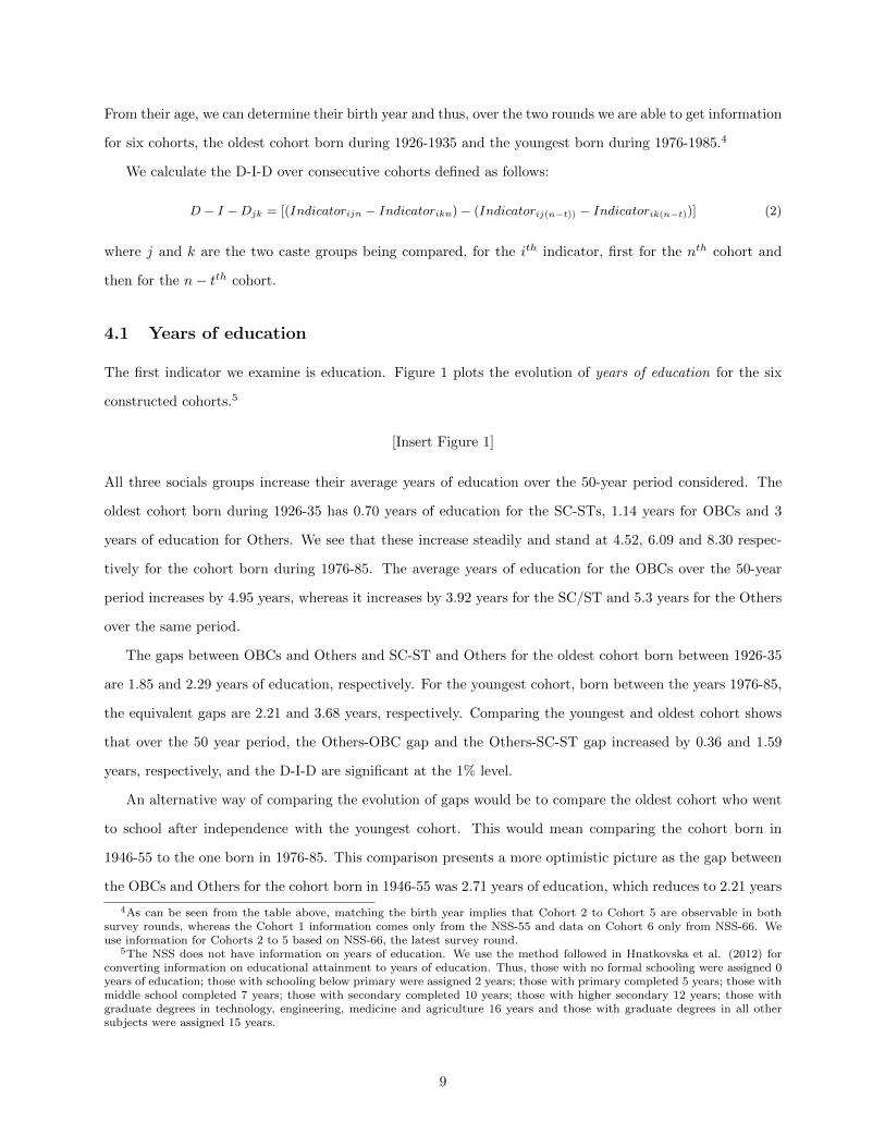
From their age, we can determine their birth year and thus, over the two rounds we are able to get information

for six cohorts, the oldest cohort born during 1926-1935 and the youngest born during 1976-1985.4

We calculate the D-I-D over consecutive cohorts defined as follows:

D − I −Djk = [(Indicatorijn − Indicatorikn) − (Indicatorij(n−t)) − Indicatorik(n−t))] (2)

where j and k are the two caste groups being compared, for the ith indicator, first for the nth cohort and

then for the n− tth cohort.

4.1 Years of education

The first indicator we examine is education. Figure 1 plots the evolution of years of education for the six

constructed cohorts.5

[Insert Figure 1]

All three socials groups increase their average years of education over the 50-year period considered. The

oldest cohort born during 1926-35 has 0.70 years of education for the SC-STs, 1.14 years for OBCs and 3

years of education for Others. We see that these increase steadily and stand at 4.52, 6.09 and 8.30 respec-

tively for the cohort born during 1976-85. The average years of education for the OBCs over the 50-year

period increases by 4.95 years, whereas it increases by 3.92 years for the SC/ST and 5.3 years for the Others

over the same period.

The gaps between OBCs and Others and SC-ST and Others for the oldest cohort born between 1926-35

are 1.85 and 2.29 years of education, respectively. For the youngest cohort, born between the years 1976-85,

the equivalent gaps are 2.21 and 3.68 years, respectively. Comparing the youngest and oldest cohort shows

that over the 50 year period, the Others-OBC gap and the Others-SC-ST gap increased by 0.36 and 1.59

years, respectively, and the D-I-D are significant at the 1% level.

An alternative way of comparing the evolution of gaps would be to compare the oldest cohort who went

to school after independence with the youngest cohort. This would mean comparing the cohort born in

1946-55 to the one born in 1976-85. This comparison presents a more optimistic picture as the gap between

the OBCs and Others for the cohort born in 1946-55 was 2.71 years of education, which reduces to 2.21 years

4As can be seen from the table above, matching the birth year implies that Cohort 2 to Cohort 5 are observable in bothsurvey rounds, whereas the Cohort 1 information comes only from the NSS-55 and data on Cohort 6 only from NSS-66. Weuse information for Cohorts 2 to 5 based on NSS-66, the latest survey round.

5The NSS does not have information on years of education. We use the method followed in Hnatkovska et al. (2012) forconverting information on educational attainment to years of education. Thus, those with no formal schooling were assigned 0years of education; those with schooling below primary were assigned 2 years; those with primary completed 5 years; those withmiddle school completed 7 years; those with secondary completed 10 years; those with higher secondary 12 years; those withgraduate degrees in technology, engineering, medicine and agriculture 16 years and those with graduate degrees in all othersubjects were assigned 15 years.

9

for the cohort born in 1976-85, whereas for the Others and SC-ST comparison, over the same time period,

there is neither divergence nor convergence.6

4.2 Other indicators of educational attainment

In order to better understand the picture of evolution of the three social groups on educational attainment,

we now look at four separate categories of education, namely, the proportion of each cohort literate or more,

has finished primary schooling or more, has finished secondary schooling or more and finally is a graduate

or has higher education, which are shown in Table 3.

[Insert Table 3]

For the category literate or more, the proportion of the cohort born in 1926-35, which was literate, was

15 percent, 25 percent and 46 percent for SC-STs, OBCs and Others, respectively. This increased to 63,

73 and 86 percent respectively for the cohort born in 1976-85. Looking at the evolution of the OBCs in

relation to Others shows a picture of steady convergence in the country, and the D-I-D estimates and their

significance are reported in Table 4. The gap between the two groups was such that that 21 percent more of

the Others were literate as compared to the OBCs for Cohort 1, and this decreases to 13 percent for Cohort

6. Comparing SC-STs to the Others also shows a pattern of convergence where the gap reduces from 31

percent more of Others being literate for Cohort 1 to 23 percent for Cohort 6.7

[Insert Table 4]

The picture for the category “primary education and more” is very similar to the picture for literacy and

more. For the cohort born in 1926-35, the proportion that has primary education or more, stands at 7, 13

and 31 percent for the SC-STs, OBCs and Others, respectively. This increases to 51, 64 and 78 percent

respectively for the Cohort 6 born in 1976-85 and aged 25-34. The gap between Cohorts 2 and 6 for the

OBCs and the Others reduces from 20 percentage points to 14 percentage points. Similarly, comparing

SC-STs with Others, the gap reduces from 32 percent to 26 percent. The convergence is especially strong

for the last 3 cohorts of the OBCs, who gain 8 percentage points relative to the Others.8

The next category of education we examine is all those with “secondary education or more”. For the

cohort born in 1926-35, 2 percent of SC-STs, 3 percent of OBCs and 13 percent of Others have secondary

6The point estimates show a gain for the SC-STs of 0.08 years of education compared to the Others, however this isstatistically not different from zero.

7If we consider the Cohort aged 15-24, i.e. those who should have achieved literacy by the time the survey was done, thegaps further reduce, and the Others have a lead of 7 percent and 13 percent over the OBCs and SC/ST, respectively.

8If we consider the Cohort aged 15-24, i.e. those who should have finished primary schooling by the time the survey wasdone, the gaps further reduce, and the Others have a lead of 9 percent and 16 percent over the OBCs and SC-STs, respectively.

10

education or more. This increases to 19, 30 and 48 percent respectively for Cohort 6 born in 1976-85.

The evolution of the OBCs and SC- STs in relation to the Others suggests that contrary to the earlier

categories, the picture for this category of education has been one of divergence rather than convergence.

Again, comparing the gap between the two groups for Cohorts 1 and 6 suggests a picture of divergence. 10

percent more of Cohort 1 had secondary education or more for the Others as compared to the OBCs. This

gap, in fact, increases to 18 percent for Cohort 6 born in 1976-85. Similarly, for SC-STs the gap increases

from 11 percent more of Others having secondary education or more for Cohort 1 to about 29 percent for

Cohort 6.

For the last category of education, those with a graduate degree or more, for the cohort born in 1926-35,

0.5 percent of SC-STs, 0.4 percent of OBCs and 4 percent of Others had a graduate degree or more. This

increases to 4.7, 9 and 20 percent respectively, for the cohort born in 1976-85 (see Table ??). Comparing

the gap between the OBCs and Others for Cohort 2 (shows that 6 percent more of Others had a graduate

degree and this gap, in fact, increases to 10.5 percent for Cohort 6 born in 1976-85, suggesting divergence in

this category of education. The SC- ST with Others comparison again shows a picture of divergence. The

gap between SC-ST and Others for the cohort born in 1935-46 (Cohort 2) was 7 percent, which increases to

15 percent for the cohort 6 born in 1976-85 (See Table 4).9

4.3 The intergenerational transmission of education

The analysis so far has been concerned with relative gains or losses on educational indicators between the

three social groups over time. We can, however, go further and also study the importance of educational

transmission across generations, and whether this differs between social groups and over the two survey

rounds considered. In particular, we want to examine whether the three social groups exhibit different levels

of intergenerational mobility. In order to do this, we match the years of education of every household head to

the years of education of the male child, for both the NSS rounds.10 We then estimate the relative measure of

intergenerational persistence in education, for the three social groups and two survey rounds, by estimating

the following equation:

Esi = α+ βEf

i +Ri + Sj +Ai + εi, (3)

9Comparing the oldest cohort that went to school after independence (cohort 3) with the youngest cohort that would havefinished schooling by 2010 (cohort 6), the D-I-D for the OBCs and SC-STs compared to the Others remains negative andsignificant.

10We identify father-son pairs based on the household identifier and ”relationship to head of household” variable. Thus, wecan only identify father-son pairs residing in the same household. Since daughters typically marry early and move to the maritalhome, NSS data does not have a mechanism to match daughters with either fathers or mothers, unless they are resident in thesame household. Most resident daughters are minors, and many are still studying, so their ultimate educational category is notknown at the point the survey is conducted.

11

where Esi and Ef

i refers to the years of education of son labelled i and father of i, respectively, Ri are the

dummies for the religious group of individual i, Sj refer to state fixed effects, Ai the age of son i, εi is the

error term. β is the parameter of interest; β measures how strongly the son’s education depends on his

father’s education. A value of 0 would imply that there is no independent effect of father’s education on the

son’s education and there is complete intergenerational mobility.

The β parameters arising from the estimation exercise are shown in Table 5. For both the survey rounds,

the intergenerational persistence of education is the strongest for SC-STs, followed by OBCs, and finally the

Others. We see that, as expected, SC-STs have the lowest levels of intergenerational mobility.

[Insert Table 5]

The fact that for these groups, fathers’ education has the biggest impact on the sons’ educational attainment

seems to suggest that “family factors” are more important for the relatively disadvantaged groups. However,

over the two survey rounds we see a decrease in the relative intergenerational persistence of education. The

average β coefficient decreases from 0.51 to 0.42 over the two NSS rounds indicating an increase in mobility

for all three social groups; hinting at an increase in equality of opportunity. Next, in order to analyze whether

the pattern of mobility is different across the social groups, we construct a dummy called Non−Backward,

which takes the value 1 if the individual belongs to the “Others” group. We then estimate the reduced form

equation given by:

Esi = α+ β1NonBackward ∗ Ef

i +NonBackward+ +β2Efi +Ri + Sj +Ai + εi.(4)

The coefficient of interest, β1, captures whether the effect of father’s education is different for the Others

group as compared to the two socially disadvantaged groups. The results are shown in Table 6 for the two

rounds. We see that β1 is negative and significant at the 1% level across the two rounds indicating, relative

to the SC-STs and OBCs, the effect of father’s education on son’s education is lower for the non-backward

group, which implies that intergenerational persistence for the social group “Others” is lower.

[Insert Table 6]

4.4 The education transition matrix

The above analysis has analysed shifts across birth cohorts. We can go further to examine generational

shifts. In order to do that, we go on to construct a matrix which depicts the transitional probabilities of the

son’s education belonging to a particular education category given the fathers level of education.

We construct six categories of education as follows: 0 representing illiterate; 1 representing literacy but

12

less than primary schooling; 2 representing more than primary schooling but less than secondary; 3 repre-

senting more than secondary but lower than higher secondary; 4 representing more than higher secondary

but lower than graduate; and 5 representing graduate education and higher. We then match the male head

of households category of education to his son’s category of education for the NSS-55 and NSS-66.

The transition matrix provides us easy visual representation of the underlying intergenerational mobil-

ity in education for the three social groups. This helps us understand whether the pattern of increasing

educational attainment which we observed above is driven by sons of household heads with high education

obtaining even higher education (i.e. intergenerational persistence), or is it due to the upward movement of

sons whose fathers had low education moving up the ladder (intergenerational mobility).

The transition matrix shown in the table below computes the probability pij the probability of a father

with education category i having a son in educational category j. A high pij where i = j represents low

intergenerational education mobility, while a high pij where i < j, would indicate high intergenerational

education mobility. The last column of the table labelled “size” shows the proportion of fathers in that

particular educational category.

So, for instance, from Table 7 we see that in NSS-55, the proportion of SC-ST fathers that were illiterate

was 59.66 percent. Given that the father was an illiterate, the probability of a son from a SC-ST family be-

ing illiterate was 40.89 percent, being literate was 11.8 percent, having primary but less than secondary was

31.68 percent, having secondary but less than higher secondary education was 8.9 percent, having more than

higher secondary but less than graduate was 4.6 percent, and finally holding a graduate degree or higher was

2.1 percent. Similarly the proportion of OBC fathers who were illiterate was 46.44 percent in 1999-2000. The

probabilities of the son being in education categories 0 to 5 were 35.75, 11.58, 34, 11.03, 5.52 and 2.1percent

respectively. Finally, 26.5 percent fathers in the Others category were illiterate, and probabilities of the son

being in categories 0 to 5 were 26.68, 12.14, 38.21, 14.14, 5.6 and 3.2 percent respectively.

[Insert Table 7]

Comparing the transitional probabilities of NSS-55 in Table 7 with those of NSS-66 in Table 8, we first

observe that for all three social groups there is an increase in the average proportion of fathers in higher

educational categories. For instance, the proportion of fathers with more than primary schooling but less

than secondary schooling increases from 17.45 to 22.85 percent, 23.98 to 29.87 percent and 27.87 to 29.80

percent for the SC-STs, OBCs and Others respectively. We also observe that for sons whose fathers had

education category 3, 4 or 5, the probability of the son achieving an educational category equal to or higher

than their father increases for all three groups, i.e. intergenerational persistence is high for families with

higher levels of education. For instance, for the probability of the father belonging to the education category

13

3 (more than secondary but lower than higher secondary) and his son belonging to the category 3, 4 or 5

increases from 73.8 to 75.9 percent, 72.8 to 85 percent and 82.1 to 87.8 percent for the SC-STs, OBCs and

Others respectively.

[Insert Table 8]

Having said this, it should be noted that conditional on fathers education, sons from the social group Others

are more likely to achieve an education category equal to or higher than their father as compared to SC-STs

and OBCs. So, for instance, in 2009-10, for fathers with education category 5 (graduate education and

higher), the probability that the son also achieves educational category 5 is 37.8, 33.56 and 54.01 percent

for the SC-ST, OBCs and Others, respectively. The reading of the matrix suggest that the ability of highly

educated parents to ensure an equivalent or higher education level for their children is best reaped by the

Others. The fact that SC-ST sons have a higher probability to be graduates and above, compared to

the OBCs, contingent upon their fathers being graduates suggests that reservations for SC-STs in higher

education might be playing a role.

4.5 Ordered probit regressions for education categories

We ran an ordered probit regression to calculate the marginal effects of being in five educational categories

defined as follows: Education category 1: not literate; category 2: literate, below primary; category 3:

primary; category 4: middle; category 5: secondary and above. Table 9 shows the probabilities of being

in each of these categories for OBCs and SC-STs relative to Others. We see that all cohorts of OBCs and

SC-STs are significantly more likely to be illiterate (category 1) than Others. The marginal effects rise

from Cohort 1 to 3 and decline thereafter, such that between Cohort 1 and 5, the likelihood of OBCs being

illiterate as compared to the Others reduces from 20.6 percent to 7.2 percent. We see a similar trend for

SC-STs as well, but first, their likelihood of being illiterate relative to Others is higher than that for OBCs

and second, the decline in this probability over successive cohorts is lower than that for OBCs.

[Insert Table 9]

For higher educational categories, the trend in probabilities changes. For category 2, i.e. literate, below

primary, we see that the three youngest cohorts of OBCs show positive marginal effects compared to the

Others, indicating convergence. For the next higher category, we see that only the two youngest cohorts

of OBCs show positive marginal effects. For the last two educational categories (middle and secondary

and above), all cohorts of OBCs are less likely to be in these categories than the Others, confirming the

D-I-D result that after the middle school level, we see divergence, rather than convergence in educational

attainment.

14

5 Occupation

How does the evolution of differences in educational attainment translate into occupational differences be-

tween groups? To start this investigation, we first estimate the number of individuals in the labor force.11

We then aggregate these individuals into three categories following a subjective classification based on

Hnatkovska et al. (2012). The rationale behind the grouping is to combine occupations that have broadly

the same skill requirements. The occupation classification that is undertaken divides individuals into three

occupational categories. Occupation 1 comprises of white-collar jobs such as administrators, executives,

managers, professionals, technical and clerical workers; Occupation 2 collects blue-collar workers such as

sales workers, service workers and production workers; Occupation 3 collects agricultural workers such as

farmers, fishermen, loggers, hunters etc.

The skill-based justification for this three-fold classification can be verified by looking at the average years

of education for individuals involved in the various occupational categories. The average years of education

for individuals involved in white-collar, blue-collar and agricultural jobs are 9.45, 5.07 and 3.41 respectively.

The difference in skill levels is also reflected in the wages earned in the three kinds of occupational groups,

with the white-collar jobs getting the highest average wage, and the agricultural occupations getting the

lowest.

The broad based classification though provides useful insights into the relationship between caste hi-

erarchy and occupational attainment or status, hides many crucial distinctions - for instance, it does not

distinguish between whether blue-collar jobs are regular wage-salaried jobs or whether they are casual or

informal. We hence complement the above exercise by additionally analyzing the evolution of regular wage

salaried (RWS) and casual jobs.

5.1 Trends in occupational categories

For the first cohort born during 1926-35, the proportion involved in agricultural jobs was 78.85 for SC-ST,

74.55 for OBCs and 71.85 for Others. Over successive cohorts, we see that for all groups, proportion of

individuals in agricultural jobs declines, to stand at 51.28, 46 and 35.46, respectively, for the cohort born

during 1966-75 and aged 35-44 in 2010.12

[Insert Table 10]

11In the NSS EUS, these are all individuals with principal activity status codes between 11 and 81.12When we trace the evolution of occupations, we focus on the oldest cohort born between 1926-35 and compare them with

the second youngest cohort born between 1966-75. The reason being that the youngest cohort born between 1976-85 are between25-34 years of age, and might be still be in a state of transition in terms of their occupational choices, whereas those bornbetween 1966-75 and aged 35-44 years would be more likely settled in their choices.

15

The proportions of SC-STs, OBCs and Others in blue-collar jobs in the oldest cohort were 17.78, 21.68 and

18.97 respectively, which have doubled for the cohort born in 1966-75 to stand at 40.4, 41.1 and 39.57. This

illustrates the shift away from agriculture towards the secondary and tertiary sectors. We also note that

gaps between groups in agricultural occupations are sharper than those for blue-collar jobs. The decline in

proportions in agricultural jobs is matched by an increase in proportions with blue-collar and white-collar

jobs, reflecting the structural shift in the economy, where the proportion of the population dependent on

agriculture is declining over the last several decades.

The caste disparities in the most prestigious category of white-collar jobs remain substantial. From 3.37

(SC-ST), 3.76 (OBC) and 9.18 (Others) percent for the cohort born in 1926-35, the shares of the three

groups stand at 8.32, 12.93 and 24.97, respectively, for the cohort born in 1966-75. Analyzing difference-in-

differences allows us to comment on whether convergence with regard to prestigious occupations is, in fact,

a reality. The shares of OBCs and SC-STs with white-collar jobs were 5.4 and 5.81 percentage points less

than the share of Others, respectively, for the cohort born in 1926-35. For the cohort born in 1966-75 (aged

35-44 in 2010), these gaps have increased to 12.04 and 16.65 percentage points, respectively. Comparing the

Others with the OBCs and SC-ST implies a D-I-D of -7% and -11%, respectively, where the differences are

significant at the 1% level. This comparison shows that occupational disparities, especially in relation to

white-collared prestigious jobs have sharpened over the time period analyzed.

A more optimistic picture emerges comparing the cohorts born between 1956-65 and 1966-75. This

comparison suggests that the OBCs have increased their share in white-collars jobs relative to the Others by

0.91 percentage points over the same time period, whereas SC-STs increased their share by 3.1 percentage

points, though the absolute share of the SC-ST remains as low as 8.3 percent compared to the 25 perecnt

for the Others. The overall picture for the OBCs shows that for cohorts born after 1946-55 the gaps in

proportion with white-collar to the Others, is decreasing or remaining constant. On the other hand, for the

SC-STs, the only instance of that convergence is when we compare those born in 1956-65 (cohort 4) and

1966-75 (cohort 5). Given the presence of quotas in public sector and government jobs, the continued lagging

behind of SC-STs possibly indicates continued gaps in the private sector.

5.1.1 Estimating probabilities of the occupational categories

We ran multinomial probit regressions separately for each cohort to estimate the probability of being in one

of the three job types (agricultural, blue-collar and white- collar) for the three caste groups. Table 11 presents

the probabilities (marginal effects) with and without controls for region, sector, and years of education for

each cohort for both rounds of NSS.

16

[Insert Table 11]

From the estimates for NSS-66, we see that SC-STs in Cohort 1 are 1.9 times less likely (without controls)

and 12.8 times less likely (with controls) be in agricultural jobs compared to Others. However, SC-STs in

Cohorts 2-5 are more likely to be in agricultural jobs compared to Others in corresponding cohorts. Similarly,

OBCs are more likely to be in agricultural jobs compared to Others in all cohorts (in regressions without

controls), but controlling for others explanatory factors, are less likely to be in agricultural jobs.

OBCs, as well as SC-STs, are less likely to be in white-collar jobs compared to Others in all cohorts,

with and without controlling for other explanatory factors. However, Table 12 shows us that the marginal

effects have by and large declined from the oldest to the youngest cohort, suggesting that the disadvantage

of younger cohorts of OBCs relative to Others appears to have decreased.

[Insert Table 12]

Comparing the marginal effects from a similar regression for NSS-55, we see that while OBCs were less likely

than Others to be in white-collar jobs also in 1999-2000, the marginal effects for the NSS-66 cohorts of OBCs

are lower, again suggesting that the relative OBC disadvantage might have reduced over the decade between

the two surveys. These regressions confirm the D-I-D trends in white-collar jobs for OBCs versus Others.

5.2 Regular wage salaried and casual jobs

The NSS divides workers into a few broad categories based on their principal activity status: own-account

worker; employer; helper in household enterprise; regular wage/ salaried employment; casual wage labor in

public works; casual wage labor in other types of work. While each of these categories merits a separate

analysis, in this paper we focus on two of the important sources of dissimilarity, viz., the proportion of all

workers that are regular wage/salaried (RWS) employees and those doing casual labor. Proportion in RWS

jobs is a good indicator of involvement in the formal sector; these jobs are coveted also because of the benefits

they confer to the worker, which are typically missing from informal sector or casual jobs. As Banerjee and

Duflo (2011) suggest, job security and regular wages seems to be one of the important aspirations of the poor

in India. Thus, the small proportions of SC- STs and OBCs in RWS jobs suggests that this is an important

facet of occupational disparity across caste groups.

We see that across all groups, the proportions engaged in RWS jobs have been rising, indicating the

greater formalization of jobs. As Table 10 shows, for the Others, there is sharp rise in the proportion in

RWS jobs from Cohort 1 to Cohort 4, but the rise is not sustained in the next two cohorts. OBCs and

SC-STs too show a much sharper rise from Cohort 1 to Cohort 4, than for the latter two cohorts. However

the percentage of RWS jobs held by the cohort aged 25-34 in 2010 are 14.51, 19.27 and 28.1 for the SC-ST,

17

OBCs and Others, respectively, indicating that economic growth has not been accompanied with access to

formal secure jobs.

Looking at the evolution and comparing the oldest to the youngest cohort shows that the difference

between the percentage of Others and OBCs having RWS jobs increases from 0.67 to 8.83 or an increase

of 8.16 percentage points and in the same time period the gap between Others and SC-ST increases by

around 13.4 percentage points. The only comparison which show convergence is comparing the cohort born

in 1966-76 to 1976-85 where relative to the Others, the OBCs and SC-ST increase their share by 3.28 and

0.62 percentage points, respectively.

Given the divergence except for the very youngest cohorts in the activity status of RWS, we explore

whether the trends in casual labor mirror those of RWS i.e. whether Others have decreased their share of

labor force in casual labor relative to the SC-ST and OBCs. Table 10 shows that not only SC-STs have

the highest proportions in casual labor, but this has in fact increased from 34.93 for Cohort 1 to 50.82 for

Cohort 6. The corresponding proportions are 16.74 to 29.94 for OBCs and 9.22 to 18.61 for Others. The

general trend in the country seems to be one of increasing proportion of the labor force employed in casual

job, which again suggests that the liberalization and economic growth have in fact eroded job security for

majority of the population.

Looking at the evolution across cohorts, we see that overall, OBCs movement across cohorts is not very

different from that of Others (D-I-D between Cohort 6 and 2 is 0.1). Between Cohorts 5 and 4, the increase

in OBC proportion in casual labor is higher than that of Others, but between Cohort 6 and 5, the increase

in proportion for Others is higher than that for OBCs, and for the other cohorts, the increase in OBC

proportions is marginally higher, so the net result, comparing OBCs and Others, is that casualisation of

labor is proceeding at a similar rate. However, the comparison between SC-STs and Others shows the trend

is exactly the opposite, in that SC-ST labor is getting into casual jobs in higher proportions across successive

cohorts compared to the Others. Comparing OBCs and SC-STs, again the rate of casualisation for SC-STs

is significantly higher than that for OBCs. Thus, the activity status profiles of the three groups continue to

look dissimilar for the three groups, with OBCs closer to the Others than to SC-STs. To sum up the

picture seems to suggest that the Others have increased the proportion of their RWS jobs as compared to the

OBCs and SC-ST (except for the youngest cohort). The trend in casualisation of labour is very similar for

Others and OBCs over the period whereas the amount of work force employed as casual labour has increased

for the SC-ST relative to the Others. The two strands of evidence suggest that there has been divergence

in the principal activity status between the Others and the OBCs and SC-ST, with the Others especially

increasing their share of the coveted RWS jobs.

18

5.3 Public sector jobs

The final occupational category we explore is the share of public sector jobs, one of the sites for affirmative

action, which in India takes the form of caste-based quotas (22.5 percent for SC-ST). Additional 27 percent

quotas for OBCs were introduced at the national level (i.e. for central government jobs) in 1990; various state

governments introduced state-specific OBC quotas at different points in time after 1950. Public sector jobs,

even those at the lowest occupational tier, are considered desirable because most offer security of tenure and

several monetary benefits, such as inflation indexation, cost-of-living adjusted pay, provident fund, pensions

and so forth. The private sector wage dispersion is larger, so there is a possibility of far greater pay at the

higher end, but the private sector is an omnibus category covering very heterogeneous establishments, with

large variability in the conditions of work and payment structures.

In Table 13 we see the evolution of public sector jobs across cohorts of the three social groups. We

concentrate on the cohorts labelled 2 to 6 from NSS-66. Table 13 shows that the SC-ST percentages with

access to public sector jobs are consistently higher than those for OBCs, which is at variance with the access

to white collar jobs, discussed above. We believe that the difference in the relative picture between SC-STs

and OBCs reflects the longer operation of SC-ST quotas. Others have the highest percentage of public

sector jobs across cohorts. The D-I-D reveals that OBCs are catching up, both with SC-STs and Others (the

evolution and statistical significance of the calculated D-I-D are shown in the online appendix). This holds

most strikingly for Cohort 4 born between the years 1956-1965, individuals who would have been between

34 and 25 years old in 1990, and hence eligible to take advantage of the new quotas. This catch-up continues

onwards to Cohort 5. We see a similar convergence between SC-ST and Others, which is in contrast to the

picture of divergence between SC-ST and Others in access to white-collar jobs.

[Insert Table 13]

Within the public sector, white and blue-collar jobs present different scenarios. The result of quotas can be

clearly seen here. Take a representative example; 6.51 percent SC-ST, 13 percent OBCs and 26.29 percent

of Cohort 4 are in white-collar jobs. But of these, 36 percent of (the 6.51) SC-ST, 21.2 percent OBCs and

24.08 percent Others are in the public sector. This reveals that there are gaps between caste groups even

within the public sector, but a much higher proportion of SC-STs owes their access to white-collar jobs to

the public sector. If there had been no quotas, SC-ST access to white collar jobs would not have been as

large as 6.51, which is already less than one-fourth the proportion of the Others. The D-I-D for white collar

public sector jobs reveals that OBCs are gaining vis-a -vis both SC-STs and Others, whereas SC-STs are

losing vis-a -vis the Others.

Thus, our suspicion that the lagging behind of the SC-STs in white collar jobs is a result of gaps in

19

the private sector is further confirmed by this picture. Of course, our data do not allow us to identify

quota beneficiaries explicitly; hence attributing the catch up to quotas is conjectural. The OBCs’ access to

white-collar jobs (both public and private), as well as public sector jobs (both blue and white-collar) shows

convergence with Others. A part of this convergence would be due to the operation of quotas but not all of it,

since there is convergence between OBCs and Others in both public and private sectors. Section 7 explicitly

examines the relationship between OBC quotas and their educational and occupational attainment.

6 Wages and labor market discrimination

The average wages for the three caste groups show the expected ranking. In 2009-10, the average daily wages

were Rs. 145, 188 and 310 for SC-STs, OBCs and Others respectively. Interestingly, for OBCs and Others,

average wages for the cohort born during 1956-65 were the highest, as this cohort is between 45 -54 years

old, at the peak of it’s earning cycle. However, for SC-STs, average wages for the cohort born in 1946-55 are

higher than for those born in 1956-65, as can be seen in the Figure 2.

[Insert Figure 2]

Comparing cohorts born in 1926-35 suggests that wage gaps between caste groups were negligible. For the

cohort born in 1966-75, the average daily wages of the Others are higher than the average daily wages of

OBCs and SC-STs by Rs. 120 and Rs. 150 respectively, indicating divergence between the three social

groups. The gaps reduce for the next cohort, but overall, comparing cohort 2, which is the oldest cohort

that went to school after Independence (born 1946-55), with Cohort 5, the D-I-D shows that both OBCs

and SC-STs have fallen behind Others in terms of average daily wages by Rs. 55 and Rs. 57 respectively,

despite some convergence occuring among the younger cohorts.13

The kernel density plots for two cohorts of SC-STs (aged 55-64 and aged 35-44) shows a rightward shift

in the distribution, confirming that the younger SC-ST cohort is doing better in terms of wages (Figure 3).

Similar plots for OBCs and Others (Figures 3) do not show this clear rightward shift - the OBC distribution

for the younger cohort is flatter and smoother; the Others distribution retains two peaks but becomes

smoother for the younger cohort.

[Insert Figure 3]

13The calculated D-I-D are significant at the 1 percent level.

20

6.1 Blinder-Oaxaca Decomposition

We perform the Blinder-Oaxaca (B-O) decomposition on the average male wage gap between Others on

the one hand, and OBCs and SC-STs respectively in order to separate the explained from the unexplained

component (the latter often treated as a proxy for labor market discrimination), the basic methodology

for which is explained in the longer version of the paper. We control for three different sets of observable

characteristics: one, personal characteristics (PC), namely, years of education, age, age squared, marital

status; two, added to PC, we control for region and sector (rural/urban) of residence 14 ; and three, added

to all these, occupation - agricultural, white-collar or blue-collar jobs. Based on NSS-66, using the pooled

model as the reference, the results of the B-O decomposition exercise between Others and OBCs can be seen

in Table 14.

[Insert Table 14]

We see that in regressions that include personal characteristics as controls (years of education, age, age

squared, married), for all cohorts between 25 to 74 years, the (geometric) means of daily log wages are Rs.

194 for Others and Rs. 135.88 for OBCs, amounting to a difference of 42.8 percent. The differences in en-

dowment account for about 62 per cent of the gap with around 38 percent remaining unexplained. Further

accounting for differences between the OBCs and Others for region of residence and sector (urban-rural)

shows that the proportion of gap that can be accounted for by differences in personal and geographical

characteristics is 61.7 percent, marginally lower than when only personal characteristics are controlled for.15

Adding additional controls for the occupation white, blue or agricultural jobs - shows that differences in

personal and geographical characteristics account for about 65.5 percent of the observed gap.

Running similar regressions for each of the cohorts separately, we see from Table 14, that the wage gap

is around 61.8 percent for the cohort aged 55-64 in 2010. The proportion of the wage gap that is explained

by differences in personal characteristics is around 81 percent, which increases to 84.5 percent with personal

characteristics combined with region, sectorial controls and occupation controls. For the cohort aged 45-54

in 2010, the observed wage gap is slightly lower, around 60.4 percent. Now differences in personal char-

acteristics can account for only 63 percent of the observed wage gap, which rises to 66 percent when we

additionally account for sector, region controls and occupational controls. Thus, from older to younger co-

horts, the absolute wage gap reduces, but the proportion that cannot be explained by differences in personal

characteristics increases.

For the cohort aged 35-44 in 2010, the observed wage gap in daily wages further reduces to 43 per cent.

14India is divided into six regions or zones, namely, East, West, South, North, Central and North-East.15India is divided into six regions or zones, namely, East, West, South, North, Central and North-East.

21

The observed differences in education and marital status can explain around 69 percent of the wage gap.

Adding controls for region, sector and occupation further increases the explained portion of the wage gap to

71.3 percent. For the youngest cohort (aged 25-34) the absolute daily wage gap amounts to around 27 per

cent, but the observed differences in endowments, occupational and geographical characteristics only explain

48 percent of the observed wage gap.

As explained in the Appendix, the decomposition estimates are sensitive to the choice of the counterfac-

tual, i.e., the assumption about the wage structure that would prevail in the absence of discrimination. The

results described in Table 14 are based on the assumption of the pooled model, where the counterfactual wage

structure is one that characterizes the whole population. Table J.1 in the Appendix shows the decomposition

results with Others’ wage structure as the counterfactual. We see that for all cohorts, the proportion of the

gap that is explained by endowments alone is smaller. This implies that, with the PC specification, if OBCs

had characteristics similar to the Others, the wage gap would be 54 percent smaller. If the labour market

treated OBCs like Others, the wage gap would be reduced by 28 percent. The interaction term captures

the combined effect of characteristics and coefficients, and shows again that if the OBCs were more like the

Others, and if the market treated them as such, the wage gap would be smaller by 18 percent. Similar to

the pooled model, we find that the absolute gap is lower for younger cohorts, but the proportion explained

by endowments also goes down, and the proportion due to coefficients (conventionally taken as a measure of

discrimination) increases as we move from older to younger cohorts.

We conduct similar decompositions between SC-ST and Others (Table 15) which reveal that the average

daily wages are Rs. 194 and Rs. 109 for Others and SC-ST, respectively, implying that the absolute wage

gap between these two groups is 77 percent.

[Insert Table 15]

Thus, the average wage gap between SC-ST and Others is a little less than twice the wage gap between OBCs

and Others. However, the unexplained proportion of the daily wage is around 39 percent which reduces to

27 percent once differences in region, sector and occupation are taken into account. The figures for each

cohort are provided in Table 15.

The above results are based on the pooled model. Table J.2 in the Appendix describes the results of the

Blinder-Oaxaca decomposition with the Others wage structure as the counterfactual. As with the pooled

model, we see that the absolute wage gaps between Others and SC-STs are higher than the corresponding

gaps between Others and OBCs, reiterating once again that SC-STs are at the bottom of the economic

hierarchy. Again the proportion of the gap explained by endowment differences is higher for SC-STs than

it is for OBCs. However, overall and for the three youngest cohorts we see that the proportion of the gap

22

explained by the interaction term is higher for SC-STs than for OBCs. This suggests that if SC-STs were

more like the Others, and if the labour market treated them more like the Others, the wage gap would be

significantly less.

The absolute wage gaps between the Others and SC-ST are higher than the gaps between Others and

OBCs for all cohorts. However, the proportion that can be explained by differences in observed characteristics

is always higher for the SC-ST as compared to the OBCs. One potential explanation could be that even

though in terms of access to schooling, the OBCs have been closing the relative gap with the Others faster

than the SC-ST, but that has not necessarily translated into convergence in quality. This implies that the

educational attainments of OBCs and Others converge, but returns (coefficients) diverge as increased access

might be masking the differences faced in schooling quality by the two groups. Similarly, our occupational

categories reflect broad differences in occupation status, and the movement of OBCs into what are classified

as white-collar jobs might be at the lower end, again implying convergence in endowments, but returns

(coefficients) could diverge as the two groups are employed in different kinds of white-collar jobs.

7 Affirmative action and occupational and educational outcomes

of OBCs

In this section we explore whether the extension of reservation since 1993 at the central level, for government

jobs and seats in universities, had any effect on the occupational and educational outcomes of the OBCs.16

In particular we explore the effect of affirmative action on three outcomes - (i) whether the individual

holds a public sector job or not (ii) whether the individual has a graduate degree or not and (iii) whether

the individual has finished secondary schooling or not.17 In order to be able to estimate the effect of the

reservation policy, we exploit the differential impact the policy had based on the age and the social group of

the individual.

The Others did not have access to reservation both before and after 1993. The SC-STs, on the other

hand, had access to reservation at the center both before and after 1993. Thus these two social groups did not

face any change in terms of affirmative action policies and form our control groups of interest. OBCs did not

have any access to reservation for central government jobs or for seats in universities prior to 1993; however

post 1993, 27 percent of all seats in government jobs and universities at the central level were reserved for

them.

The first two dependent variables of interest were affected directly by the policy change and are natural

16The policy change was announced in 1991, but it was implemented from 1993.17In India finishing secondary schooling amounts to finishing 10 years of schooling, where the 10th year involves nationally

conducted exams.

23

outcomes to explore. Whether an individual has finished secondary schooling or not is an other key outcome

as most public sector jobs in India require the individual to have finished at least 10 years of schooling.18

Our basic empirical strategy consists of using a difference-in-differences estimator to calculate the impact

of the extension of affirmative action on the younger OBC cohorts who would potentially benefit from

the policy change. Given that the reservation involved provision of government jobs and university seats,

any individual who was OBC and under the age of 16 in 1993, could possibly alter his educational and

occupational choice in response to the policy change. We thus label all individuals who were 16 and younger

in 1993 as the younger cohort and those who were older than 16 in 1993 as the older cohort. Given the

nature of the policy change, the younger OBC cohorts faced a change in policy whereas the younger cohorts

of SC-STs and Others did not.

The finding of a differential trend for the younger OBC cohorts could be interpreted as the effect of a

change in the reservation policy only under the assumption that in the absence of the policy change the

trends among the groups would have been identical. In order to check for pre-policy trends among the three

social groups, we estimate a reduce form placebo regression given by:

Oijkn = Tk +OBCi + SC − STi + δ1OBCi ∗ Tk + δ2SCSTi ∗ Tk + Sn + εijkn, (5)

where Oijkn refers to the three outcomes of interest of individual i from group j from cohort k and state n.

Tk is a cohort dummy which takes the value 1 in case the individual is greater than 18 years old and less than

28 years in 1993.19 The older cohort consists of individuals aged 29 to 53 in 1993. OBCi and SCSTi are

dummies which take the value 1 in case individual i belongs to the OBC or the SC-ST group (the omitted

category is the Others) and Sn is a set of state dummies. δ1 and δ2 the coefficient on the interaction of the

cohort dummy with the OBC and SC-ST dummy, respectively, is capturing whether the younger OBC and

SC-ST cohorts have a differential trend with respect to the younger cohorts belonging to the Others. If our

identification assumption is correct then δ1 = δ2 = 0 , which would reflect that the three groups exhibit

identical trends prior to 1993. The results of the estimation exercise are shown in Table 16, and all standard

errors are clustered at the level of the state.

[Insert Table 16]

In column (1) the dependent variable is a dummy for whether the individual holds a public sector job or

not. Inspecting the coefficients on the two interaction terms shows that δ1 = δ2 = 0, implying there were

18In India government jobs are divided into Class I, II, III and IV jobs. Class IV jobs include jobs such as lower divisionclerks, drivers, technicians/mechanics, electricians, canteen staff etc. and have the requirement of the individual to have finishedsecondary schooling.

19Observe these are individuals who did not really benefit from the policy change and is intended as a placebo test.

24

no differential trends between the Others and OBCs and SC-STs. In column (2) the dependent variable is a

dummy for whether the individual has a graduate degree or not. We see that the OBCs exhibit no differential

trend with respect to the Others, whereas the coefficient on the SC-ST interaction term shows that the SC-

ST were falling behind the Others in the number of people who are university graduates. Finally column

(3) again shows that the OBCs and SC-ST have identical trends with respect to the Others in terms of the

individuals who finish secondary schooling. To sum up, we cannot reject the null hypothesis of identical

trends between the OBCs and Others for a period of 35 years before the policy change in 1993 on all three

outcomes considered, whereas for the SC-ST the assumption of identical trends is only fulfilled for public

sector jobs and secondary education.

Having first verified that the assumption of identical trends is satisfied (for 5 of the 6 cases), we again

estimate Eqaution 5 but now, Tk, the cohort dummy takes the value 1 when the individual is aged 16 or less

in 1993. We consider the treated cohort to be individuals aged 1 to 16 in 1993 (or 18 to 33 in 2010) and

the older cohort to be individuals aged 17 to 43 in 1993 (or 34 to 60 in 2010). The results of the estimation

exercise are shown in Table 17, where all errors are clustered at the state level.

[Insert Table 17]

In column (1) the dependent variable is whether the individual hold a public sector job. Inspecting the

coefficient on the interaction of the younger cohort dummy with the OBC dummy shows that is positive and

statistically significant at the 1% level. The coefficient shows that extension of affirmative action increased

the share of OBCs holding a public sector job by 2.6 percentage points. Reassuringly the interaction term

on the coefficient of the SC-ST dummy with the younger cohort dummy is close to zero and statistically

insignificant, as it should be if our identifying assumption is correct.

In column (2) the dependent variable is whether the individual holds a graduate degree or not. The

coefficient on the interaction of the younger cohort dummy with both the OBC and SC-ST is close to zero

and insignificant. This suggests that the policy of reserving seats in higher educational institutions has not

had the intended effect.

In column (3) the dependent variable is a dummy for whether the individual has finished secondary

schooling or not. The coefficient on the interaction of the younger cohort dummy with the OBC dummy

is positive and statistically significant, and indicates that affirmative action increased the number of OBC

individuals finishing secondary schooling by 4 percentage points. This is consistent with the channel of

individuals having to obtain at least 10 years of schooling to obtain a public sector job. Again the coefficient

on the SC-ST dummy with the cohort dummy is statistically insignificant again providing support for our

underlying identifying assumption.

25

The above results show that extension of affirmative action increased the share of OBCs with secure

public sector jobs. However, they also show that the OBCs have been unable to make use of the quotas in

higher education. One potential explanation could be that the quality of primary and secondary schooling

is so low that individuals are unable to reach the stage where they can benefit from reservation in higher

educational institutions. The fact that the affirmative action also increased the share of individuals who

hold secondary schooling seems to indicate that we are actually capturing the effect of affirmative action at

work. As noted before at least 10 years or more of schooling are required to be eligible for even the lowest

tier (or Class IV) government jobs, hence the fact that we observe both increase in share of public sector

jobs as well as share of secondary schools, and that the increase in the share of secondary school graduates

(4 percentage points) is greater than the share of those obtaining government jobs (2.6 percentage points)

is consistent with the hypothesized channel.

8 Regional differences in outcomes: Does political representation

play a role? A preliminary analysis

The results from the previous section show there remain wide disparities between the three social groups on

most socio-economic indicators, and the process of convergence has been limited to certain fields (literacy

and primary education, blue collar jobs), and especially to the younger cohorts. In this section, we analyze if

there are any regional differences in the trends on the various indicators for the OBCs born over the period

1926-85. Additionally, this exercise also tries to understand if political representation might help explain the

observed patterns of regional differences in the socio-economic evolution of the OBCs.

Jaffrelot (2003) groups the various Indian states into seven categories or types based on changes in

OBC representation in respective state assemblies. The seven types are as follows: Type I comprising

Uttar Pradesh, Madhya Pradesh and Bihar, where the share of upper caste MLAs has steadily declined.

These states, particularly Bihar, saw a sharp rise in OBC MLAs post-1990; Type II comprising Punjab,

Rajasthan and Gujarat, where OBC proportion among MLAs is low, except in Gujarat. These states have

the same proportions of upper-caste MLAs as the Type I states, but the dominant castes among OBCs are

economically as strong, and on the rise; Type 3 comprising Maharashtra, Karnataka and Andhra Pradesh.

In this group, the dominant castes, i.e. the peasant proprietary castes alone are powerful. In Karnataka and

Andhra Pradesh, these are classified as OBCs, but not in Maharashtra; Type 4 comprising Jharkhand and

Chhattisgarh. These are predominantly tribal states. Here OBCs are 20 percent of the population but 30

percent of the MLAs; Type 5 comprising West Bengal and Kerala. These are two states where upper castes

26

have resisted the rise of the OBCs. West Bengal is the only state in the country where the proportion of

upper-caste MLAs has increased over the years; Type 6 comprising Himachal Pradesh and Delhi. These are

states where the share of OBC MLAs is low but is proportional to their share in the population; and Type 7

comprising Tamil Nadu. This is also a case of quasi-proportionality, like the Type 6 states, except that the

share of OBC MLAs is high.20 The evolution of the share of the upper caste as members of the legislative

assembly (MLA) is shown in Table 18.

[Insert Table 18]

We are interested in analyzing whether increased political representation has been associated with better

outcomes for OBCs, so we exploit the differences in OBC representation across the seven types to examine

this question. In order to keep our analysis simple, we concentrate on two important indicators, namely,

proportion with graduate degree or higher and the cohort share of white-collar jobs.

Looking at the share of OBCs with graduate education or more for the first cohort that went to school

after independence (Cohort 3 born between 1946-55) in Table 19 we see that the Types V (West Bengal

and Kerala) and VII (Tamil Nadu) do the best with around 3.8% of the cohort having a graduate degree or

higher. This proportion is around 1.5 percent for the Types I (Uttar Pradesh, Madhya Pradesh and Bihar),

II (Punjab, Rajasthan and Gujarat) and III (Maharashtra, Karnataka and Andhra Pradesh) and as low as

0.4 percent for the Type VI (Himachal Pradesh and Delhi). However, the picture changes dramatically for

the youngest cohort born between the years 1976-85.

[Insert Table 19]

The Types I and II perform the worst with only 5.9 percent and 5.3 percent, respectively, of the cohort

holding a graduate degree or higher. On the other hand, the states classified as Types III, V, VI and VII

see an increase in the share of OBCs with graduate degree or more, and have a share of greater than 11.5

percent. On the other hand, for the Others, the trend does not seem to be identical. They perform the

best in Tamil Nadu with almost 45 percent of the youngest cohort having a graduate degree and then have

21.2, 22.4, 20.7, 11.9 and 28.4 percent as graduates in the Types I, II, III, V and VI, respectively. The

D-I-D comparing the OBCs and Others for Cohorts 3 and 6 show that the OBCs gain relative to Others

in the Types III, V and VI by 1, 7 and 3 percentage points, respectively, and lose ground by 5, 8 and 3

percentage points in Types I, II and VII. The states in which the OBCs lose ground namely Uttar Pradesh,

Bihar, Madhya Pradesh, Punjab, Rajasthan and Gujarat include the key northern states, for which Jaffrelot

puts forth the hypothesis of the “silent revolution”, mentioned in the beginning of the paper. However,

20We in our analysis ignore the Type 4 states as they were created only in the year 2000.

27

our analysis suggests that at least in the field of higher education the OBCs in these states do not see a

translation of their political ascendancy into better outcomes, and in fact, have tended to trail behind their

counterparts in other states. A final point worth mentioning is that states in which the OBCs perform the

worst (Types I and II), their relative share of graduates compared to the better performing states (Types III,

V and VI) is around half, whereas for the Others a similar comparison reveals a small advantage in terms of

share of graduates in the Type I and II states.

[Insert Table 20]

In the case of the prestigious white collar jobs (see Table 20) comparing the cohort born in 1946-55 to the

cohort born in 1966-75 we see a similar picture as for the case of graduate education with the OBCs in

Type I and II states relatively underperforming as compared to the OBCs in state Types III, V, VI and VII.

The D-I-D comparing the cohort aged 35-44 to the cohort aged 55-64 for the OBCs and Others, however,

shows that the OBCs increase their relative share in white collar jobs in all six types of states with the

greatest gains in Tamil Nadu. However, here we observe the relative gains to be largest in the states of

Uttar Pradesh, Bihar, Madhya Pradesh (Type I) and Punjab, Rajasthan and Gujarat, as compared to the

Type III, V and VI states. It is important to note that although the gains for OBCs on white collar jobs

have been larger in the north Indian states in absolute amounts, they still have the lowest share as compared

to the other categories or types. In sum, our preliminary analysis seems to indicate that the link between

increased political representation and socio-economic outcomes for the OBCs seem tenuous at best, for the

indicators of graduate education and white-collar jobs.

9 Conclusion

Summing up, our findings suggest that the gaps between the Others and OBCs and SC-ST remain large for

a variety of important indicators. Average MPCE and wages of the OBCs and SC-ST are 57 and 69 per

cent and 57 and 42 per cent, respectively, of the average of the Others. Their share of labor force employed

in white-collar jobs is about one fourth and half the proportion of the Others. On the other hand, the

share of the OBC and SC-ST labor force employed as casual labor is twice and thrice that of the Others,

respectively. However, despite significant gaps in the above indicators, we find evidence of catch- up between

OBCs and Others for the younger cohorts (especially in literacy, primary education and wages), but we find

continued divergence in all education categories after the middle school level, regular wage salaried jobs and

in white-collar jobs except for the youngest cohort.

This picture is different from the one that emerges after a similar analysis between SC-STs and Others,

28

where the divergence and dissimilarity in all indicators vis-a-vis the Others is much greater. In the case

of intergenerational transmission of education we find the lowest mobility for SC-STs though there is an

increase over time. Younger cohorts of OBCs are closer to the Others than to SC-STs in several indicators,

whereas the older cohorts were closer to the SC-STs. Analysis of the affirmative action policies instituted for

the OBCs since 1993 are seen to increase both their share of government jobs and the proportion finishing

secondary schooling. We also carry out a preliminary exploration of the role of political representation in

affecting socio-economic outcomes of the OBCs, and find little evidence in support of it.

References

Banerjee, Abhijit Vinayak and Esther Duflo, Poor economics: A radical rethinking of the way to fight

global poverty, PublicAffairs, 2011.

Deshpande, Ashwini, “Overlapping identities under liberalization: Gender and caste in India,” Economic

Development and Cultural Change, 2007, 55 (4), 735–760.

, The Grammar of Caste: Economic Discrimination in Contemporary India, Oxford University Press,

2011.

Galanter, Marc, Competing equalities: law and the backward classes in India, University of California

Press Berkeley, 1984.

Gupta, Dipankar, Caste in question: identity or hierarchy?, Vol. 12, SAGE Publications India, 2009.

Hnatkovska, Viktoria, Amartya Lahiri, and Sourabh Paul, “Castes and labor mobility,” American

Economic Journal: Applied Economics, 2012, 4 (2), 274–307.

Iyer, Lakshmi, Tarun Khanna, and Ashutosh Varshney, “Caste and Entrepreneurship in India,”

Economic and Political Weekly, 2013, 48 (6), 52–60.

Jaffrelot, Christophe, India’s silent revolution: the rise of the lower castes in North India, Orient Black-

swan, 2003.

Madheswaran, S and Paul Attewell, “Caste discrimination in the Indian urban labour market: Evidence

from the National Sample Survey,” Economic and Political Weekly, 2007, pp. 4146–4153.

Zacharias, Ajit and Vamsi Vakulabharanam, “Caste stratification and wealth inequality in India,”

World Development, 2011, 39 (10), 1820–1833.

29

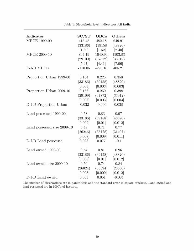
Table 1: Household level indicators: All India

Indicator SC/ST OBCs OthersMPCE 1999-00 415.48 482.18 649.91

(33186) (39158 (48820)[1.39] [1.62] [2.40]

MPCE 2009-10 864.19 1040.94 1503.83(29109) (37872) (33912)[5.47] [4.41] [7.96]

D-I-D MPCE -110.05 -295.16 405.21

Proportion Urban 1999-00 0.164 0.225 0.358(33186) (39158) (48820)[0.003] [0.003] [0.003]

Proportion Urban 2009-10 0.166 0.259 0.398(29109) (37872) (33912)[0.003] [0.003] [0.003]

D-I-D Proportion Urban -0.032 -0.006 0.038

Land possessed 1999-00 0.58 0.83 0.97(33186) (39158) (48820)[0.009] [0.01] [0.012]

Land possessed size 2009-10 0.48 0.71 0.77(26246) (35128) (31407)[0.007] [0.009] [0.011]

D-I-D Land possessed 0.023 0.077 -0.1

Land owned 1999-00 0.54 0.81 0.96(33186) (39158) (48820)[0.008] [0.01] [0.012]

Land owned size 2009-10 0.50 0.74 0.84(26024) (33394) (28660)[0.008] [0.009] [0.012]

D-I-D Land owned 0.033 0.051 -0.084

The number of observations are in parenthesis and the standard error in square brackets. Land owned andland possessed are in 1000’s of hectares.

30

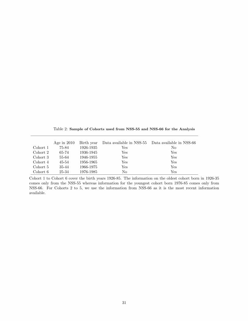
Table 2: Sample of Cohorts used from NSS-55 and NSS-66 for the Analysis

Age in 2010 Birth year Data available in NSS-55 Data available in NSS-66Cohort 1 75-84 1926-1935 Yes NoCohort 2 65-74 1936-1945 Yes YesCohort 3 55-64 1946-1955 Yes YesCohort 4 45-54 1956-1965 Yes YesCohort 5 35-44 1966-1975 Yes YesCohort 6 25-34 1976-1985 No Yes

Cohort 1 to Cohort 6 cover the birth years 1926-85. The information on the oldest cohort born in 1926-35comes only from the NSS-55 whereas information for the youngest cohort born 1976-85 comes only fromNSS-66. For Cohorts 2 to 5, we use the information from NSS-66 as it is the most recent informationavailable.

31

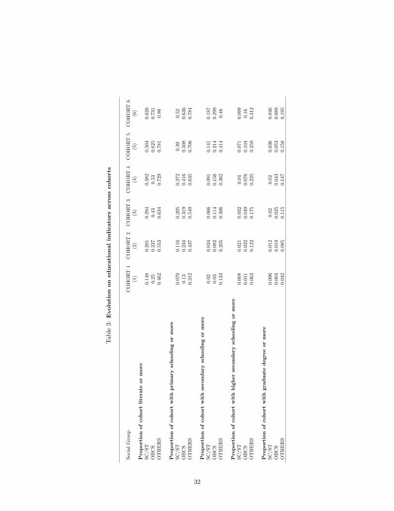
Tab

le3:

Evolu

tion

on

educati

onal

indic

ato

rsacro

sscohort

s

Soci

alG

rou

pC

OH

OR

T1

CO

HO

RT

2C

OH

OR

T3

CO

HO

RT

4C

OH

OR

T5

CO

HO

RT

6(1

)(2

)(3

)(4

)(5

)(6

)P

rop

ort

ion

of

coh

ort

lite

rate

or

more

SC

/ST

0.14

80.2

010.2

940.3

820.

504

0.62

6O

BC

S0.

250.

337

0.43

0.5

30.

625

0.731

OT

HE

RS

0.462

0.553

0.634

0.72

90.

781

0.86

Pro

port

ion

of

coh

ort

wit

hp

rim

ary

sch

ooli

ng

or

more

SC

/ST

0.07

90.1

160.2

050.2

720.3

90.

52O

BC

S0.

130.

234

0.31

90.

416

0.50

80.

636

OT

HE

RS

0.312

0.437

0.549

0.63

50.

706

0.78

4

Pro

port

ion

of

coh

ort

wit

hse

con

dary

sch

ooli

ng

or

more

SC

/ST

0.02

0.03

40.

066

0.09

10.

141

0.18

7O

BC

S0.

030.

082

0.11

40.

156

0.21

40.

299

OT

HE

RS

0.133

0.205

0.306

0.36

20.

414

0.48

Pro

port

ion

of

coh

ort

wit

hh

igh

er

secon

dary

sch

ooli

ng

or

more

SC

/ST

0.00

80.0

210.0

320.

040.

071

0.09

9O

BC

S0.0

110.0

320.

049

0.07

60.

104

0.16

OT

HE

RS

0.063

0.122

0.175

0.22

50.

259

0.31

2

Pro

port

ion

of

coh

ort

wit

hgra

du

ate

degre

eor

more

SC

/ST

0.00

60.0

120.

020.

02

0.03

60.

046

OB

CS

0.0

040.0

190.

025

0.04

30.

053

0.089

OT

HE

RS

0.042

0.085

0.115

0.14

70.

158

0.19

5

32

Tab

le4:

Evolu

tion

of

D-I

-Don

sele

cte

deducati

onal

indic

ato

rs

D-I

-D(C

OH

OR

T(2

-1))

D-I

-D(C

OH

OR

T(3

-2))

D-I

-D(C

OH

OR

T(4

-3))

D-I

-D(C

OH

OR

T(5

-4))

D-I

-D(C

OH

OR

T(6

-5))

(1)

(2)

(3)

(4)

(5)

Years

of

ed

ucati

on

OB

Cvs

Oth

ers

-0.3

6***

-0.5

***

-0.0

80.

16*

**0.4

2***

(0.0

8)(0

.10)

(0.0

8)

(0.0

7)

(0.0

6)

SC

/ST

vs

Oth

ers

-0.9

1***

-0.5

6***

-0.3

9***

0.3

4***

0.14

***

(0.1

3)(0

.11)

(0.0

8)

(0.0

7)

(0.0

6)

Lit

era

cy

or

more

OB

Cvs

Oth

ers

-0.0

040.

012

0.0

050.

042**

*0.

028**

*(0

.008

)(0

.01)

(0.0

08)

(0.0

06)

(0.0

05)

SC

/ST

vs

Oth

ers

-0.0

380.

011

-0.0

060.

069**

*0.

044**

*(0

.015

)(0

.011

)(0

.008

)(0

.007

)(0

.006)

Gra

du

ate

or

more

OB

Cvs

Oth

ers

-0.0

28**

*-0

.025*

**-0

.013

***

-0.0

01-0

.001

(0.0

05)

(0.0

05)

(0.0

04)

(0.0

04)

(0.0

04)

SC

/ST

vs

Oth

ers

-0.0

37**

*-0

.022*

**-0

.032

***

0.0

05**

*-0

.027

***

(0.0

06)

(0.0

06)

(0.0

05)

(0.0

04)

(0.0

04)

33

Table 5: Estimates of intergenerational persistence in education

SC-ST (NSS-55) SC-ST (NSS-66) OBCs (NSS-55) OBCs (NSS-66) OTHERS (NSS-55) OTHERS (NSS-66)Integen. Coeff. (β) 0.543*** 0.423*** 0.513*** 0.422*** 0.480*** 0.409***

(0.010) (0.008) (0.008) (0.007) (0.005) (0.006)State Dummies Yes Yes Yes Yes Yes Yes

Religion Dummies Yes Yes Yes Yes Yes Yes

Age Yes Yes Yes Yes Yes Yes

Observations 11,820 11,227 16,746 15,421 22,555 14,851

R-squared 0.23 0.25 0.26 0.26 0.37 0.35

Standard errors in parentheses. *** p<0.01, ** p<0.05, * p<0.1.

Table 6: Differnces in intergenerational persistence in education between socially backward and non-backward groups

NSS -55 NSS -66Intergenerational Coeff * Non Backward Dummy (β1) -0.057*** -0.026***

(0.006) (0.008)Non Backward Dummy 1.40*** 1.20***

(0.054) (0.063)Integenerational Coefficient (β3) 0.543*** 0.438***

(0.006) (0.005)State Dummies Yes Yes

Religion Dummies Yes Yes

Age Yes Yes

Observations 51,121 41,499

R-squared 0.34 0.31

Standard errors in parentheses. *** p<0.01, ** p<0.05, * p<0.1.

34

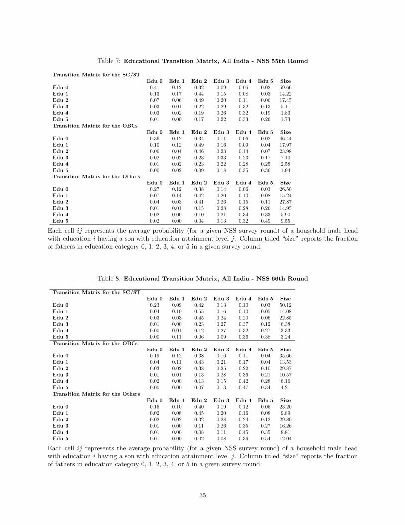
Table 7: Educational Transition Matrix, All India - NSS 55th Round

Transition Matrix for the SC/STEdu 0 Edu 1 Edu 2 Edu 3 Edu 4 Edu 5 Size

Edu 0 0.41 0.12 0.32 0.09 0.05 0.02 59.66Edu 1 0.13 0.17 0.44 0.15 0.08 0.03 14.22Edu 2 0.07 0.06 0.49 0.20 0.11 0.06 17.45Edu 3 0.03 0.01 0.22 0.29 0.32 0.13 5.11Edu 4 0.03 0.02 0.19 0.26 0.32 0.19 1.83Edu 5 0.01 0.00 0.17 0.22 0.33 0.26 1.73Transition Matrix for the OBCs

Edu 0 Edu 1 Edu 2 Edu 3 Edu 4 Edu 5 SizeEdu 0 0.36 0.12 0.34 0.11 0.06 0.02 46.44Edu 1 0.10 0.12 0.49 0.16 0.09 0.04 17.97Edu 2 0.06 0.04 0.46 0.23 0.14 0.07 23.98Edu 3 0.02 0.02 0.23 0.33 0.23 0.17 7.10Edu 4 0.01 0.02 0.23 0.22 0.28 0.25 2.58Edu 5 0.00 0.02 0.09 0.18 0.35 0.36 1.94Transition Matrix for the Others

Edu 0 Edu 1 Edu 2 Edu 3 Edu 4 Edu 5 SizeEdu 0 0.27 0.12 0.38 0.14 0.06 0.03 26.50Edu 1 0.07 0.14 0.42 0.20 0.10 0.08 15.24Edu 2 0.04 0.03 0.41 0.26 0.15 0.11 27.87Edu 3 0.01 0.01 0.15 0.28 0.28 0.26 14.95Edu 4 0.02 0.00 0.10 0.21 0.34 0.33 5.90Edu 5 0.02 0.00 0.04 0.13 0.32 0.49 9.55

Each cell ij represents the average probability (for a given NSS survey round) of a household male headwith education i having a son with education attainment level j. Column titled “size” reports the fractionof fathers in education category 0, 1, 2, 3, 4, or 5 in a given survey round.

Table 8: Educational Transition Matrix, All India - NSS 66th Round

Transition Matrix for the SC/STEdu 0 Edu 1 Edu 2 Edu 3 Edu 4 Edu 5 Size

Edu 0 0.23 0.09 0.42 0.13 0.10 0.03 50.12Edu 1 0.04 0.10 0.55 0.16 0.10 0.05 14.08Edu 2 0.03 0.03 0.45 0.24 0.20 0.06 22.85Edu 3 0.01 0.00 0.23 0.27 0.37 0.12 6.38Edu 4 0.00 0.01 0.12 0.27 0.32 0.27 3.33Edu 5 0.00 0.11 0.06 0.09 0.36 0.38 3.24Transition Matrix for the OBCs

Edu 0 Edu 1 Edu 2 Edu 3 Edu 4 Edu 5 SizeEdu 0 0.19 0.12 0.38 0.16 0.11 0.04 35.66Edu 1 0.04 0.11 0.43 0.21 0.17 0.04 13.53Edu 2 0.03 0.02 0.38 0.25 0.22 0.10 29.87Edu 3 0.01 0.01 0.13 0.28 0.36 0.21 10.57Edu 4 0.02 0.00 0.13 0.15 0.42 0.28 6.16Edu 5 0.00 0.00 0.07 0.13 0.47 0.34 4.21Transition Matrix for the Others

Edu 0 Edu 1 Edu 2 Edu 3 Edu 4 Edu 5 SizeEdu 0 0.15 0.10 0.40 0.19 0.12 0.05 23.20Edu 1 0.02 0.08 0.45 0.20 0.16 0.08 9.89Edu 2 0.02 0.02 0.32 0.28 0.24 0.12 29.80Edu 3 0.01 0.00 0.11 0.26 0.35 0.27 16.26Edu 4 0.01 0.00 0.08 0.11 0.45 0.35 8.81Edu 5 0.01 0.00 0.02 0.08 0.36 0.54 12.04

Each cell ij represents the average probability (for a given NSS survey round) of a household male headwith education i having a son with education attainment level j. Column titled “size” reports the fractionof fathers in education category 0, 1, 2, 3, 4, or 5 in a given survey round.

35

Tab

le9:

Marg

inal

Eff

ect

of

SC

/ST

and

OB

Cdum

my

inord

ere

dpro

bit

regre

ssio

nfo

reducati

on

cate

gori

es

AL

LC

OH

OR

TS

CO

HO

RT

1C

OH

OR

T2

CO

HO

RT

3C

OH

OR

T4

CO

HO

RT

5C

OH

OR

T6

Coh

ort

2to

1C

ohor

t3

to2

Coh

ort

4to

3C

ohor

t5

to4

Coh

ort

6to

5C

ohort

5to

1E

du

1SC

/ST

0.30

7***

0.32

4***

0.3

47**

*0.

366

***

0.31

4***

0.26

8***

0.15

5***

0.02

30.

019

-0.0

52-0

.046

-0.1

13-0

.056

(0.0

0)(0

.00)

(0.0

0)(0

.00)

(0.0

0)(0

.00)

(0.0

0)(0

.00)

(0.0

0)(0

.00)

(0.0

0)(0

.00)

(0.0

0)

OB

Cs

0.19

1***

0.20

8***

0.231

***

0.22

9***

0.19

6***

0.14

7***

0.07

2***

0.02

3-0

.002

-0.0

33-0

.049

-0.0

75-0

.061

(0.0

0)(0

.00)

(0.0

0)(0

.00)

(0.0

0)(0

.00)

(0.0

0)(0

.00)

(0.0

0)(0

.00)

(0.0

0)(0

.00)

(0.0

0)

Edu

2SC

/ST

-0.0

01**

*-0

.061

***

-0.0

38*

**-0

.020

***

0.00

5***

0.02

7***

0.03

0***

0.02

30.

018

0.02

50.

022

0.00

30.0

88

(0.0

0)(0

.00)

(0.0

0)(0

.00)

(0.0

0)(0

.00)

(0.0

0)(0

.00)

(0.0

0)(0

.00)

(0.0

0)(0

.00)

(0.0

0)

OB

Cs

0.00

6***

-0.0

30**

*-0

.016*

**-0

.003

***

0.01

1***

0.02

1***

0.01

6***

0.01

40.

013

0.01

40.

01-0

.005

0.0

51

(0.0

0)(0

.00)

(0.0

0)(0

.00)

(0.0

0)(0

.00)

(0.0

0)(0

.00)

(0.0

0)(0

.00)

(0.0

0)(0

.00)

(0.0

0)

Edu

3SC

/ST

-0.0

30**

*-0

.076

***

-0.0

65*

**-0

.055

***

-0.0

25*

**0.

004*

**0.0

20**

*0.

011

0.01

0.03

0.02

90.

016

0.0

8(0

.00)

(0.0

0)(0

.00)

(0.0

0)

(0.0

0)(0

.00)

(0.0

0)(0

.00)

(0.0

0)(0

.00)

(0.0

0)(0

.00)

(0.0

0)

OB

Cs

-0.0

11**

*-0

.044

***

-0.0

37**

*-0

.027

***

-0.0

08**

*0.

011*

**0.

013*

**0.

007

0.01

0.01

90.

019

0.00

20.0

55

(0.0

0)(0

.00)

(0.0

0)(0

.00)

(0.0

0)(0

.00)

(0.0

0)(0

.00)

(0.0

0)(0

.00)

(0.0

0)(0

.00)

(0.0

0)

Edu

4SC

/ST

-0.0

67**

*-0

.062

***

-0.0

74*

**-0

.082

***

-0.0

71*

**-0

.051

***

-0.0

44**

*-0

.012

-0.0

080.

011

0.02

0.00

70.0

11

(0.0

0)(0

.00)

(0.0

0)(0

.00)

(0.0

0)(0

.00)

(0.0

0)(0

.00)

(0.0

0)(0

.00)

(0.0

0)(0

.00)

(0.0

0)

OB

Cs

-0.0

38**

*-0

.041

***

-0.0

48**

*-0

.049

***

-0.0

40**

*-0

.023

***

-0.0

18**

*-0

.007

-0.0

010.

009

0.01

70.

005

0.0

18

(0.0

0)(0

.00)

(0.0

0)(0

.00)

(0.0

0)(0

.00)

(0.0

0)(0

.00)

(0.0

0)(0

.00)

(0.0

0)(0

.00)

(0.0

0)

Edu

5SC

/ST

-0.2

09**

*-0

.124

***

-0.1

71*

**-0

.209

***

-0.2

22*

**-0

.248

***

-0.1

62**

*-0

.047

-0.0

38-0

.013

-0.0

260.

086

-0.1

24

(0.0

0)(0

.00)

(0.0

0)(0

.00)

(0.0

0)(0

.00)

(0.0

0)(0

.00)

(0.0

0)(0

.00)

(0.0

0)(0

.00)

(0.0

0)

OB

Cs

-0.1

47**

*-0

.093

***

-0.1

30**

*-0

.151

***

-0.1

59**

*-0

.156

***

-0.0

83**

*-0

.037

-0.0

21-0

.008

0.00

30.

073

-0.0

63

(0.0

0)(0

.00)

(0.0

0)(0

.00)

(0.0

0)(0

.00)

(0.0

0)(0

.00)

(0.0

0)(0

.00)

(0.0

0)(0

.00)

(0.0

0)

Pan

el(a

)re

por

tsth

em

ragi

nal

effec

tsof

the

SC

/S

Tan

dO

BC

du

mm

yin

an

op

der

edp

rob

itre

gre

ssio

nof

edu

cati

on

cate

gori

es1

to5

on

aco

nst

ant

and

anS

C/S

Tan

dO

BC

du

mm

yfo

rea

chco

hor

t.P

an

el(b

)of

the

tab

lere

port

sth

ech

an

ge

inth

em

arg

inal

effec

tsov

ersu

cces

sive

coh

ort

san

dov

erth

een

tire

sam

ple

per

iod

.S

tan

dar

der

rors

are

inp

are

nth

esis

.*

p-v

alu

e0.1

0,

**

p-v

alu

e0.0

5,

***

p-v

alu

e0.0

1.

36

Table 10: Evolution on occupational categories of interest across cohorts

Social Group COHORT 1 COHORT 2 COHORT 3 COHORT 4 COHORT 5 COHORT 6(1) (2) (3) (4) (5) (6)

% empl in agricultural jobsSC/ST 78.85 65.7 65.47 56.58 51.28 53.58OBCS 74.55 67.01 58.52 49.1 45.98 44.25OTHERS 71.85 65.69 48.35 37.55 35.46 35

% empl in blue collar jobsSC/ST 17.78 28.95 28.1 36.9 40.4 39.51OBCS 21.68 24.4 31.21 37.56 41.1 40.86OTHERS 18.97 18.27 28.02 36.16 39.57 39.96

% empl in white collar jobsSC/ST 3.4 5.4 6.4 6.5 8.3 6.9OBCS 3.8 8.6 10.3 13.3 12.9 14.9OTHERS 9.2 16 23.6 26.3 25 25

% empl in RWS jobsSC/ST 2.1 2.18 10.53 15.18 13.56 14.51OBCS 1.66 4.66 9.91 16.04 15.66 19.27OTHERS 2.33 3.69 18.65 27.02 27.77 28.1

% empl in casual labor jobsSC/ST 34.93 37.66 40.51 46.54 49.23 50.82OBCS 16.74 19.74 25.55 28.64 32.39 29.94OTHERS 9.22 8.51 13.33 15.45 15.79 18.61

Cohort 1 is the cohort born between the years 1926-35 and the data comes from NSS-55. The Cohorts 2 to6 are born between the years 1936-85 and are from the NSS-66. The total time period covered is cohortsborn between 1926-85.

37

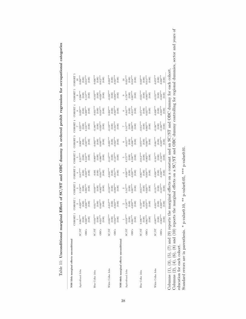
Tab

le11

:U

ncondit

ional

marg

inal

Eff

ect

of

SC

/ST

and

OB

Cdum

my

inord

ere

dpro

bit

regre

ssio

nfo

roccupati

onal

cate

gori

es

NS

S55th

marg

inal

eff

ects

un

con

dit

ion

al

CO

HO

RT

1C

OH

OR

T1

CO

HO

RT

2C

OH

OR

T3

CO

HO

RT

3C

OH

OR

T3

CO

HO

RT

4C

OH

OR

T4

CO

HO

RT

5C

OH

OR

T5

12

34

56

78

910

Agr

icu

ltu

ral

Job

sS

C/S

T0.0

61**

*-0

.020**

*0.1

58***

0.017***

0.2

17**

*0.

008*

**0.

225

***

0.0

29***

0.2

06***

0.05

0**

*(0

.00)

(0.0

0)

(0.0

0)

(0.0

0)

(0.0

0)

(0.0

0)

(0.0

0)(0

.00)

(0.0

0)(0

.00)

OB

Cs

0.0

20***

-0.0

26**

*0.0

95**

*-0

.023*

**

0.133*

**

-0.0

27***

0.135

***

0.009

***

0.11

2***

0.0

15***

(0.0

0)(0

.00)

(0.0

0)

(0.0

0)

(0.0

0)

(0.0

0)

(0.0

0)(0

.00)

(0.0

0)(0

.00)

Blu

eC

olla

rJob

sS

C/S

T-0

.016*

**0.

031**

*-0

.048***

-0.0

01

-0.0

69**

*-0

.002

***

-0.1

06**

*-0

.031

***

-0.1

03**

*-0

.026

***

(0.0

0)(0

.00)

(0.0

0)

(0.0

0)

(0.0

0)

(0.0

0)

(0.0

0)(0

.00)

(0.0

0)(0

.00)

OB

Cs

0.0

24***

0.0

49**

*-0

.002*

**

0.034***

-0.0

06*

**0.

049

***

-0.0

29*

**

0.01

8***

-0.0

29**

*0.0

12*

**(0

.00)

(0.0

0)

(0.0

0)

(0.0

0)

(0.0

0)

(0.0

0)

(0.0

0)(0

.00)

(0.0

0)(0

.00)

Wh

ite

Col

lar

Job

sS

C/S

T-0

.045**

*-0

.012***

-0.1

10***

-0.0

16***

-0.1

47*

**

-0.0

05*

**

-0.1

19*

**

0.0

02**

*-0

.103*

**-0

.024*

**(0

.00)

(0.0

0)

(0.0

0)

(0.0

0)

(0.0

0)

(0.0

0)

(0.0

0)(0

.00)

(0.0

0)(0

.00)

OB

Cs

-0.0

44**

*-0

.023*

**

-0.0

92*

**

-0.0

11*

**

-0.1

27**

*-0

.022

***

-0.1

05**

*-0

.027

***

-0.0

82**

*-0

.027

***

(0.0

0)(0

.00)

(0.0

0)

(0.0

0)

(0.0

0)

(0.0

0)

(0.0

0)(0

.00)

(0.0

0)(0

.00)

NS

S66th

marg

inal

eff

ects

un

con

dit

ion

al

12

34

56

78

910

Agr

icu

ltu

ral

Job

sS

C/S

T-0

.019

***

-0.1

28***

0.147***

-0.0

28**

*0.1

75**

*-0

.015*

**

0.1

47*

**

-0.0

41**

*0.

176**

*0.

024*

**(0

.00)

(0.0

0)

(0.0

0)

(0.0

0)

(0.0

0)

(0.0

0)

(0.0

0)(0

.00)

(0.0

0)(0

.00)

OB

Cs

0.0

01***

-0.0

59**

*0.0

87**

*-0

.028*

**

0.106*

**

-0.0

06***

0.098

***

-0.0

15**

*0.

087*

**

0.0

16***

(0.0

0)(0

.00)

(0.0

0)

(0.0

0)

(0.0

0)

(0.0

0)

(0.0

0)(0

.00)

(0.0

0)(0

.00)

Blu

eC

olla

rJob

sS

C/S

T0.

106*

**

0.159***

-0.0

17**

*0.0

67***

-0.0

14*

**

0.0

75*

**

-0.0

11***

0.071

***

-0.0

21**

*0.

049*

**

(0.0

0)(0

.00)

(0.0

0)

(0.0

0)

(0.0

0)

(0.0

0)

(0.0

0)(0

.00)

(0.0

0)(0

.00)

OB

Cs

0.0

61***

0.0

79**

*0.

020***

0.0

58**

*-0

.002*

**

0.0

36*

**

0.002

***

0.0

37**

*-0

.005*

**0.

014

***

(0.0

0)(0

.00)

(0.0

0)

(0.0

0)

(0.0

0)

(0.0

0)

(0.0

0)(0

.00)

(0.0

0)(0

.00)

Wh

ite

Col

lar

Job

sS

C/S

T-0

.087**

*-0

.031***

-0.1

31***

-0.0

38***

-0.1

61*

**

-0.0

61*

**

-0.1

36*

**

-0.0

30*

**-0

.155*

**-0

.073*

**(0

.00)

(0.0

0)

(0.0

0)

(0.0

0)

(0.0

0)

(0.0

0)

(0.0

0)(0

.00)

(0.0

0)(0

.00)

OB

Cs

-0.0

63**

*-0

.020*

**

-0.1

07*

**

-0.0

30*

**

-0.1

03**

*-0

.029

***

-0.1

00**

*-0

.023

***

-0.0

82**

*-0

.030

***

(0.0

0)(0

.00)

(0.0

0)

(0.0

0)

(0.0

0)

(0.0

0)

(0.0

0)(0

.00)

(0.0

0)(0

.00)

Col

um

ns

(1),

(3),

(5),

(7)

and

(9)

rep

orts

the

marg

inal

effec

tson

aco

nst

ant

an

dan

SC

/S

Tan

dO

BC

du

mm

yfo

rea

chco

hort

.C

olu

mn

s(2

),(4

),(6

),(8

)an

d(1

0)re

por

tsth

em

arg

inal

effec

tson

aS

C/S

Tan

dO

BC

du

mm

yco

ntr

oll

ing

for

regio

nal

du

mm

ies,

sect

or

an

dye

ars

of

edu

cati

onfo

rea

chco

hor

t.S

tan

dar

der

rors

are

inp

aren

thes

is.

*p

-val

ue0

.10,

**

p-v

alu

e0.0

5,

***

p-v

alu

e0.0

1.

38

Tab

le12

:C

hanges

inuncondit

ional

marg

inal

Eff

ect

of

SC

/ST

and

OB

Cdum

my

inord

ere

dpro

bit

regre

ssio

nfo

roccupati

onal

cate

gori

es

NS

S55th

chan

ges

inm

arg

inal

eff

ects

Coh

ort

2to

1C

ohor

t2

to1

Coh

ort

3to

2C

oh

ort

3to

2C

ohort

4to

3C

ohort

4to

3C

ohor

t5

to4

Coh

ort

5to

4C

ohor

t5

to1

Coh

ort

5to

11

23

45

67

89

10A

gric

ult

ura

lJob

sS

C/S

T0.0

97

0.037

0.0

59

-0.0

09

0.0

080.

021

-0.0

190.

021

0.145

0.07

OB

Cs

0.075

0.0

03

0.0

38-0

.004

0.002

0.0

36-0

.023

0.006

0.09

20.

041

Blu

eC

olla

rJob

sS

C/S

T-0

.032

-0.0

32-0

.021

-0.0

01

-0.0

37-0

.029

0.00

30.0

05-0

.087

-0.0

57O

BC

-0.0

26-0

.015

-0.0

04

0.0

15

-0.0

23-0

.031

0-0

.006

-0.0

53

-0.0

37

Wh

ite

Col

lar

Job

sS

C/S

T-0

.065

-0.0

04-0

.037

0.011

0.028

0.0

070.

016

-0.0

26-0

.058

-0.0

12O

BC

-0.0

480.

012

-0.0

35

-0.0

110.

022

-0.0

05

0.023

0-0

.038

-0.0

04

NS

S66th

chan

ges

inm

arg

inal

eff

ects

Agr

icu

ltu

ral

Job

sS

C/S

T0.1

66

0.1

0.028

0.0

13

-0.0

28

-0.0

260.0

29

0.06

5-0

.176

-0.0

24O

BC

s0.

086

0.0

31

0.0

190.

022

-0.0

08

-0.0

09

-0.0

110.

031

-0.0

87-0

.016

Blu

eC

olla

rJob

sS

C/S

T-0

.123

-0.0

920.0

03

0.008

0.0

03-0

.004

-0.0

1-0

.022

0.02

1-0

.049

OB

Cs

-0.0

41-0

.021

-0.0

22

-0.0

22

0.004

0.0

01-0

.007

-0.0

230.

005

-0.0

14

Wh

ite

Col

lar

Job

sS

C/S

T-0

.044

-0.0

07-0

.03

-0.0

23

0.02

50.

031

-0.0

19-0

.043

0.15

50.0

73O

BC

s-0

.044

-0.0

10.

004

0.0

01

0.0

030.

006

0.0

18

-0.0

070.

082

0.03

Col

um

ns

(1),

(3),

(5),

(7)

and

(9)

rep

orts

the

chan

ge

inm

arg

inal

effec

tson

aco

nst

ant

an

dan

SC

/S

Tan

dO

BC

du

mm

yfo

rea

chco

hort

.C

olu

mn

s(2

),(4

),(6

),(8

)an

d(1

0)re

por

tsth

ech

an

ge

inm

arg

inal

effec

tson

aS

C/S

Tan

dO

BC

du

mm

yco

ntr

oll

ing

for

regio

nal

du

mm

ies,

sect

or

an

dye

ars

ofed

uca

tion

for

each

coh

ort.

Not

eal

lch

ange

sar

esi

gnifi

cant

atth

e1%

leve

l.

39

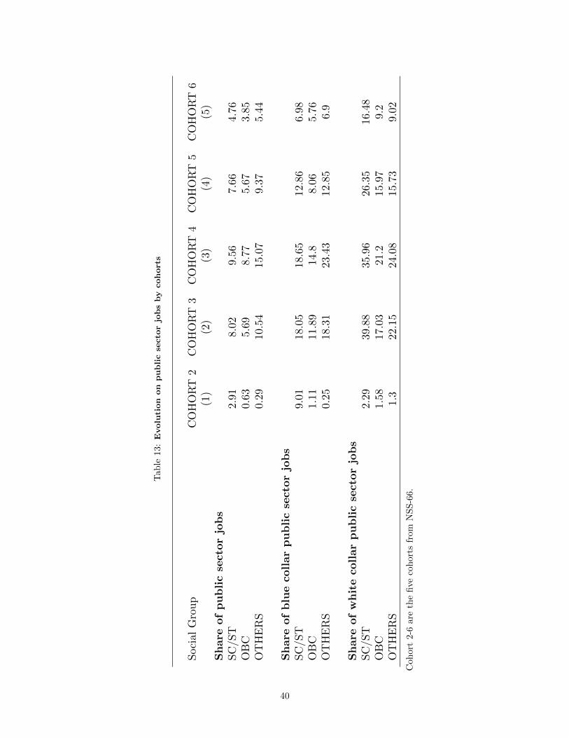
Tab

le13:

Evolu

tion

on

public

secto

rjo

bs

by

cohort

s

Soci

alG

rou

pC

OH

OR

T2

CO

HO

RT

3C

OH

OR

T4

CO

HO

RT

5C

OH

OR

T6

(1)

(2)

(3)

(4)

(5)

Sh

are

of

pu

blic

secto

rjo

bs

SC

/ST

2.9

18.0

29.5

67.

66

4.7

6O

BC

0.6

35.6

98.7

75.6

73.

85

OT

HE

RS

0.2

910.

54

15.0

79.3

75.4

4

Sh

are

of

blu

ecollar

pu

bli

cse

cto

rjo

bs

SC

/ST

9.0

118

.05

18.

65

12.8

66.9

8O

BC

1.1

111.8

914

.88.0

65.7

6O

TH

ER

S0.2

518.

31

23.4

312

.85

6.9

Sh

are

of

wh

ite

collar

pu

bli

cse

cto

rjo

bs

SC

/ST

2.2

939

.88

35.

96

26.3

516.4

8O

BC

1.5

817.0

321

.215.

97

9.2

OT

HE

RS

1.3

22.

15

24.0

815

.73

9.0

2

Coh

ort

2-6

are

the

five

coh

orts

from

NSS

-66.

40

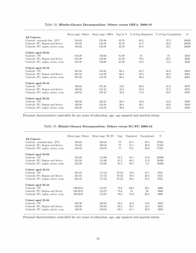
Table 14: Blinder-Oaxaca Decomposition: Others versus OBCs: 2009-10

Mean wage: Others Mean wage: OBCs Gap in % % of Gap Explained % of Gap Unexplained NAll CohortsControls - personal char. (PC) 194.02 135.88 42.78 62.5 37.5 28033Controls: PC, Region and Sector 194.02 135.88 42.78 61.7 38.3 28033Controls: PC, region, sector, occp. 194.02 135.88 42.78 65.5 34.5 28033

Cohort aged 55-64Controls - PC 216.28 133.60 61.89 81 19 2638Controls: PC, Region and Sector 216.28 133.60 61.89 79.5 20.5 2638Controls: PC, region, sector, occp. 216.28 133.60 61.89 84.5 15.5 2638

Cohort aged 45-54Controls - PC 231.83 144.50 60.4 63.7 36.3 6664Controls: PC, Region and Sector 231.83 144.50 60.4 63.5 36.5 6664Controls: PC, region, sector, occp. 231.83 144.50 60.4 66.2 33.8 6664

Cohort aged 35-44Controls - PC 196.92 137.42 43.2 68.8 31.2 8978Controls: PC, Region and Sector 196.92 137.42 43.2 72.6 27.4 8978Controls: PC, region, sector, occp. 196.92 137.42 43.2 71.3 28.7 8978

Cohort aged 25-34Controls - PC 169.38 133.58 26.8 45.6 54.3 9350Controls: PC, Region and Sector 169.38 133.58 26.8 36.1 63.9 9350Controls: PC, region, sector, occp. 169.38 133.58 26.8 47.6 52.3 9350

Personal characteristics controlled for are years of education, age, age squared and marital status.

Table 15: Blinder-Oaxaca Decomposition: Others versus SC/ST: 2009-10

Mean wage: Others Mean wage: SC-ST Gap Explained Unexplained NAll CohortsControls - personal char. (PC) 194.02 109.58 77 61.5 38.5 27321Controls: PC, Region and Sector 194.02 109.58 77 71.1 28.9 27321Controls: PC, region, sector, occp. 194.02 109.58 77 73.1 26.9 27321

Cohort aged 55-64Controls - PC 216.28 112.96 91.5 84.1 15.9 26490Controls: PC, Region and Sector 216.28 112.96 91.5 88.1 11.9 26490Controls: PC, region, sector, occp. 216.28 112.96 91.5 92.7 7.3 26490

Cohort aged 45-54Controls - PC 231.83 117.53 97.23 74.9 25.1 6521Controls: PC, Region and Sector 231.83 117.53 97.23 79.5 20.5 6521Controls: PC, region, sector, occp. 231.83 117.53 97.23 83.5 16.5 6521

Cohort aged 35-44Controls - PC 196.9213 113.27 73.8 60.9 39.1 8660Controls: PC, Region and Sector 196.9213 113.27 73.8 74 26 8660Controls: PC, region, sector, occp. 196.9213 113.27 73.8 73.2 26.8 8660

Cohort aged 25-34Controls - PC 169.38 103.62 63.5 45.2 54.8 9282Controls: PC, Region and Sector 169.38 103.62 63.5 56.7 43.3 9282Controls: PC, region, sector, occp. 169.38 103.62 63.5 61.1 38.9 9282

Personal characteristics controlled for are years of education, age, age squared and marital status.

41

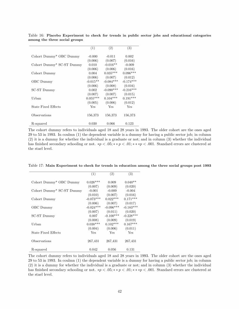
Table 16: Placebo Experiment to check for trends in public sector jobs and educational categoriesamong the three social groups

(1) (2) (3)

Cohort Dummy* OBC Dummy -0.000 -0.011 0.002(0.006) (0.007) (0.016)

Cohort Dummy* SC-ST Dummy 0.010 -0.016** -0.009(0.006) (0.006) (0.016)

Cohort Dummy 0.004 0.035*** 0.096***(0.006) (0.007) (0.012)

OBC Dummy -0.015** -0.084*** -0.174***(0.006) (0.008) (0.016)

SC-ST Dummy 0.002 -0.090*** -0.216***(0.007) (0.007) (0.015)

Urban 0.055*** 0.104*** 0.191***(0.005) (0.006) (0.012)

State Fixed Effects Yes Yes Yes

Observations 156,373 156,373 156,373

R-squared 0.030 0.066 0.123

The cohort dummy refers to individuals aged 18 and 28 years in 1993. The older cohort are the ones aged29 to 53 in 1993. In coulmn (1) the dependent variable is a dummy for having a public sector job; in column(2) it is a dummy for whether the individual is a graduate or not; and in column (3) whether the individualhas finished secondary schooling or not. ∗p < .05; ∗ ∗ p < .01; ∗ ∗ ∗p < .001. Standard errors are clustered atthe stael level.

Table 17: Main Experiment to check for trends in education among the three social groups post 1993

(1) (2) (3)

Cohort Dummy* OBC Dummy 0.026*** 0.009 0.040**(0.007) (0.009) (0.020)

Cohort Dummy* SC-ST Dummy -0.001 -0.009 -0.004(0.010) (0.007) (0.016)

Cohort Dummy -0.073*** 0.022*** 0.171***(0.006) (0.007) (0.017)

OBC Dummy -0.024*** -0.096*** -0.183***(0.007) (0.011) (0.020)

SC-ST Dummy 0.007 -0.100*** -0.228***(0.008) (0.009) (0.019)

Urban 0.038*** 0.102*** 0.167***(0.004) (0.006) (0.011)

State Fixed Effects Yes Yes Yes

Observations 267,431 267,431 267,431

R-squared 0.042 0.056 0.131

The cohort dummy refers to individuals aged 18 and 28 years in 1993. The older cohort are the ones aged29 to 53 in 1993. In coulmn (1) the dependent variable is a dummy for having a public sector job; in column(2) it is a dummy for whether the individual is a graduate or not; and in column (3) whether the individualhas finished secondary schooling or not. ∗p < .05; ∗ ∗ p < .01; ∗ ∗ ∗p < .001. Standard errors are clustered atthe stael level.

42

Table 18: Evolution of the OBC MLAs (state-wise %)

States % in 1952 1955- 1960- 1967 1969- 1971- 1975- 1980- 1984- 1987- 1991- 1993- 1996- 2001- 2007State 57 63 70 74 79 83 85 90 92 95 2000 05

PopulationType IUttar Pradesh 41.7 9.0 12 13 29.2 26.8 18.3 16.8 13.4 19.6 24.2 27.1 32.4 24.8 27.5 -Madhya Pradesh 41.5 - 4.7 9.1 9.4 - 9.5 14.3 16.1 18.6 18.7 - 22.7 22.0 19.5 -Bihar 38.5 20.6 19.4 24.4 26.6 27.9 25.7 28.3 30.4 - 34.9 - 46.8 40.3 42 -Type IIPunjab - - - - - - - 3.4 - - - 5.1 - 3.4 3.4 -Rajasthan 40 3.7 2.5 4.4 2.2 5.5 2.5 7.4 8 12 - 5.2 - 6.6 8.9 -Gujarat 40 - - 8 11 - 16 15 24 24 26 - 21 21 29 34Type IIIMaharashtra 29.8 - - - 22.3 - 21.4 23.2 19.7 24.6 26 - 23.2 23.6 23.9 -Karnataka 32.5 7.3 13.1 14.1 11.2 - 12.6 13 13 10 13.9 - 12.8 12.5 - -Andhra Pradesh 36 - 8.7 13 14.3 - 19.5 19 20.7 20.1 11.9 - 12.9 11.9 18.3 -Type IVJharkand 19.7 - - - - - - - - - - - - 27.2 29.7 -Chhattisgarh 50.4 - - - - - - - - - - - - - 23.3 -Type VWest Bengal - 0 0 0 0 0 0 0 0 0 0 0 0 - - -Kerala - - 27 26 33 30 - 20 26 27 28 25 - 29 31 -Type VIHimachal Pradesh 10.5 - - - 1.7 - 2.9 5.9 7.4 5.9 7.4 - 10.3 7.4 7.4 -Delhi 14 - - - - - - - - - - - 7 7 7 -Type VIITamil Nadu 63.6 - - - 66.2 - 61.6 59 57.7 56.9 61.5 62.4 - 62 - -

Source (Jaffrelot, 2003).

43

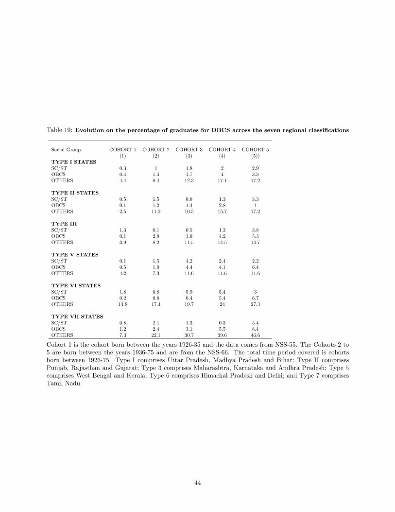
Table 19: Evolution on the percentage of graduates for OBCS across the seven regional classifications

Social Group COHORT 1 COHORT 2 COHORT 3 COHORT 4 COHORT 5(1) (2) (3) (4) (5))

TYPE I STATESSC/ST 0.3 1 1.8 2 2.9OBCS 0.4 1.4 1.7 4 3.3OTHERS 4.4 8.4 12.3 17.1 17.2

TYPE II STATESSC/ST 0.5 1.5 0.8 1.3 3.3OBCS 0.1 1.2 1.4 2.8 4OTHERS 2.5 11.2 10.5 15.7 17.2

TYPE IIISC/ST 1.3 0.1 0.5 1.3 3.8OBCS 0.1 2.8 1.9 4.2 5.3OTHERS 3.9 8.2 11.5 14.5 14.7

TYPE V STATESSC/ST 0.1 1.5 4.2 2.4 2.2OBCS 0.5 1.9 4.4 4.1 6.4OTHERS 4.2 7.3 11.6 11.6 11.6

TYPE VI STATESSC/ST 1.8 0.8 5.9 5.4 3OBCS 0.2 0.8 0.4 5.4 6.7OTHERS 14.8 17.4 19.7 24 27.3

TYPE VII STATESSC/ST 0.8 2.1 1.3 0.3 5.4OBCS 1.2 2.4 3.1 5.5 8.4OTHERS 7.3 22.1 30.7 39.6 46.6

Cohort 1 is the cohort born between the years 1926-35 and the data comes from NSS-55. The Cohorts 2 to5 are born between the years 1936-75 and are from the NSS-66. The total time period covered is cohortsborn between 1926-75. Type I comprises Uttar Pradesh, Madhya Pradesh and Bihar; Type II comprisesPunjab, Rajasthan and Gujarat; Type 3 comprises Maharashtra, Karnataka and Andhra Pradesh; Type 5comprises West Bengal and Kerala; Type 6 comprises Himachal Pradesh and Delhi; and Type 7 comprisesTamil Nadu.

44

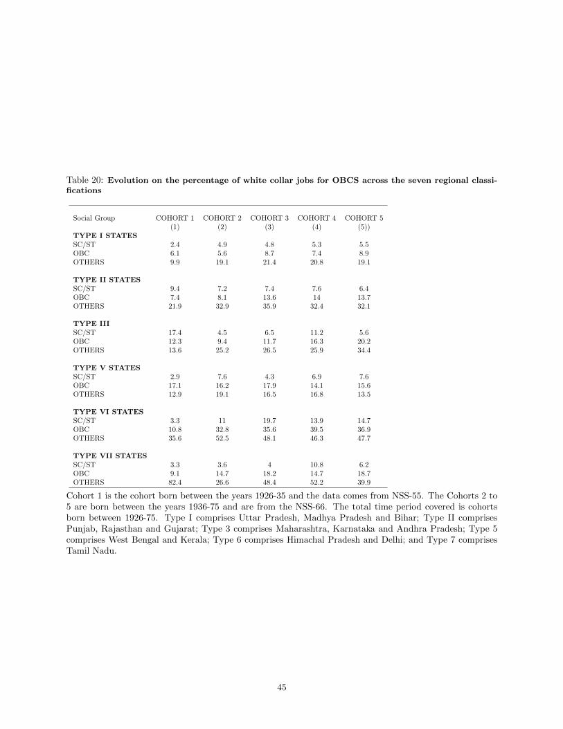
Table 20: Evolution on the percentage of white collar jobs for OBCS across the seven regional classi-fications

Social Group COHORT 1 COHORT 2 COHORT 3 COHORT 4 COHORT 5(1) (2) (3) (4) (5))

TYPE I STATESSC/ST 2.4 4.9 4.8 5.3 5.5OBC 6.1 5.6 8.7 7.4 8.9OTHERS 9.9 19.1 21.4 20.8 19.1

TYPE II STATESSC/ST 9.4 7.2 7.4 7.6 6.4OBC 7.4 8.1 13.6 14 13.7OTHERS 21.9 32.9 35.9 32.4 32.1

TYPE IIISC/ST 17.4 4.5 6.5 11.2 5.6OBC 12.3 9.4 11.7 16.3 20.2OTHERS 13.6 25.2 26.5 25.9 34.4

TYPE V STATESSC/ST 2.9 7.6 4.3 6.9 7.6OBC 17.1 16.2 17.9 14.1 15.6OTHERS 12.9 19.1 16.5 16.8 13.5

TYPE VI STATESSC/ST 3.3 11 19.7 13.9 14.7OBC 10.8 32.8 35.6 39.5 36.9OTHERS 35.6 52.5 48.1 46.3 47.7

TYPE VII STATESSC/ST 3.3 3.6 4 10.8 6.2OBC 9.1 14.7 18.2 14.7 18.7OTHERS 82.4 26.6 48.4 52.2 39.9

Cohort 1 is the cohort born between the years 1926-35 and the data comes from NSS-55. The Cohorts 2 to5 are born between the years 1936-75 and are from the NSS-66. The total time period covered is cohortsborn between 1926-75. Type I comprises Uttar Pradesh, Madhya Pradesh and Bihar; Type II comprisesPunjab, Rajasthan and Gujarat; Type 3 comprises Maharashtra, Karnataka and Andhra Pradesh; Type 5comprises West Bengal and Kerala; Type 6 comprises Himachal Pradesh and Delhi; and Type 7 comprisesTamil Nadu.

45

0.70 1.08

1.79

2.40

3.50

4.62

1.14

2.07

2.85

3.76

4.70

6.09

3.00

4.28

5.56

6.56

7.33

8.30

0.00  

1.00  

2.00  

3.00  

4.00  

5.00  

6.00  

7.00  

8.00  

9.00  

Cohort  1   Cohort  2   Cohort  3   Cohort  4   Cohort  5   Cohort  6  

SC/ST  

OBCS  

OTHERS  

Fig. 1: Years of Education across cohorts

Cohort 1 are born between the years 1926-35 and Cohort 6 between 1976-85. The gap between the OBCsand Others for Cohort 1 and Cohort 6 are 1.85 and 2.21 years, respectively. This implies the D-I-D is

-0.36*** years.The gap between the SC-ST and Others for Cohort 1 and Cohort 6 are 2.29 and 3.68 years,respectively. This implies the D-I-D is -1.59*** years. The gap between the OBCs and Others for Cohort

3 and Cohort 6 are 2.71 and 2.21 years, respectively. This implies the D-I-D is 0.50*** years. The gapbetween the SC-ST and Others for Cohort 1 and Cohort 6 are 3.76 and 3.68 years, respectively. This

implies the D-I-D is 0.08 years. * p-value - 0.10, ** p-value - 0.05, *** p-value - 0.01.

46

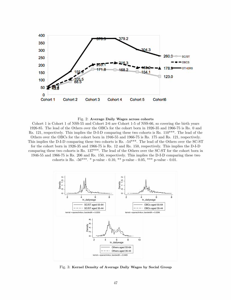
Fig. 2: Average Daily Wages across cohorts

Cohort 1 is Cohort 1 of NSS-55 and Cohort 2-6 are Cohort 1-5 of NSS-66, so covering the birth years1926-85. The lead of the Others over the OBCs for the cohort born in 1926-35 and 1966-75 is Rs. 0 andRs. 121, respectively. This implies the D-I-D comparing these two cohorts is Rs. 110***. The lead of theOthers over the OBCs for the cohort born in 1946-55 and 1966-75 is Rs. 175 and Rs. 121, respectively.

This implies the D-I-D comparing these two cohorts is Rs. -54***. The lead of the Others over the SC-STfor the cohort born in 1926-35 and 1966-75 is Rs. 12 and Rs. 150, respectively. This implies the D-I-D

comparing these two cohorts is Rs. 137***. The lead of the Others over the SC-ST for the cohort born in1946-55 and 1966-75 is Rs. 206 and Rs. 150, respectively. This implies the D-I-D comparing these two

cohorts is Rs. -56***. * p-value - 0.10, ** p-value - 0.05, *** p-value - 0.01.

0.5

11.

52

Dens

ity

2 4 6 8ln_dailywage

SC/ST aged 55-64SC/ST aged 35-44

kernel = epanechnikov, bandwidth = 0.0250

0.5

11.

52

Dens

ity

2 4 6 8ln_dailywage

OBCs aged 55-64OBCs aged 35-44

kernel = epanechnikov, bandwidth = 0.0296

0.2

.4.6

.8De

nsity

2 4 6 8 10ln_dailywage

Others aged 55-64Others aged 35-44

kernel = epanechnikov, bandwidth = 0.0485

Fig. 3: Kernel Density of Average Daily Wages by Social Group

47

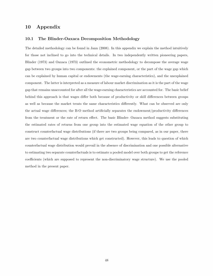
10 Appendix

10.1 The Blinder-Oaxaca Decomposition Methodology

The detailed methodology can be found in Jann (2008). In this appendix we explain the method intuitively

for those not inclined to go into the technical details. In two independently written pioneering papers,

Blinder (1973) and Oaxaca (1973) outlined the econometric methodology to decompose the average wage

gap between two groups into two components: the explained component, or the part of the wage gap which

can be explained by human capital or endowments (the wage-earning characteristics), and the unexplained

component. The latter is interpreted as a measure of labour market discrimination as it is the part of the wage

gap that remains unaccounted for after all the wage-earning characteristics are accounted for. The basic belief

behind this approach is that wages differ both because of productivity or skill differences between groups

as well as because the market treats the same characteristics differently. What can be observed are only

the actual wage differences; the B-O method artificially separates the endowment/productivity differences

from the treatment or the rate of return effect. The basic Blinder- Oaxaca method suggests substituting

the estimated rates of returns from one group into the estimated wage equation of the other group to

construct counterfactual wage distributions (if there are two groups being compared, as in our paper, there

are two counterfactual wage distributions which get constructed). However, this leads to question of which

counterfactual wage distribution would prevail in the absence of discrimination and one possible alternative

to estimating two separate counterfactuals is to estimate a pooled model over both groups to get the reference

coefficients (which are supposed to represent the non-discriminatory wage structure). We use the pooled

method in the present paper.

48

Table J.1: Blinder-Oaxaca Decomposition: Others versus OBCs: 2009-10

Mean wages: Others Mean wages: OBCs Gap (%) % endowments % coefficients % interaction NAll CohortsControls: personal characteristics (PC) 194.03 135.89 42.79 53.75 28.03 18.24 28033Controls: PC+region+sector 194.03 135.89 42.79 52.17 26.7 21.15 28033Controls: PC+region+sector+occp 194.03 135.89 42.79 57.53 22.82 19.67 28033

Cohort aged 55-64Controls: personal characteristics (PC) 216.29 133.6 61.9 73.33 11.75 14.93 2638Controls: PC+region+sector 216.29 133.6 61.9 69.3 10.62 19.07 2638Controls: PC+region+sector+occp 216.29 133.6 61.9 76.26 7.27 16.49 2638

Cohort aged 45-54Controls: personal characteristics (PC) 231.84 144.51 60.44 54.13 25.65 20.24 6664Controls: PC+region+sector 231.84 144.51 60.44 57.14 26.93 15.95 6664Controls: PC+region+sector+occp 231.84 144.51 60.44 60.33 23.34 16.34 6664

Cohort aged 35-44Controls: personal characteristics (PC) 196.93 137.43 43.29 58.97 19.11 21.94 8978Controls: PC+region+sector 196.93 137.43 43.29 60.53 12.56 26.92 8978Controls: PC+region+sector+occp 196.93 137.43 43.29 60.55 13.99 25.47 8978

Cohort aged 25-34Controls: personal characteristics (PC) 169.39 133.59 26.8 39.99 47.96 12.07 9350Controls: PC+region+sector 169.39 133.59 26.8 27.76 51.71 20.55 9350Controls: PC+region+sector+occp 169.39 133.59 26.8 41.67 41.29 17.06 9350

Personal characteristics controlled for are years of education, age, age squared and marital status.

Table J.2: Blinder-Oaxaca Decomposition: Others versus SC-STs: 2009-10

Mean wages: Others Mean wages: SCSTs Gap (%) % endowments % coefficients % interaction NAll CohortsControls: personal characteristics (PC) 194.03 109.59 77.05 47.08 26.09 26.85 273321Controls: PC+region+sector 194.03 109.59 77.05 58.75 18.08 23.19 273321Controls: PC+region+sector+occp 194.03 109.59 77.05 65.16 18.69 16.17 273321

Cohort aged 55-64Controls: personal characteristics (PC) 216.29 112.97 91.47 82.32 14.03 3.66 2490Controls: PC+region+sector 216.29 112.97 91.47 88.8 9.93 1.29 2490Controls: PC+region+sector+occp 216.29 112.97 91.47 95.67 6.95 -2.61 2490

Cohort aged 45-54Controls: personal characteristics (PC) 231.84 117.54 97.24 61.52 15.42 23.07 6521Controls: PC+region+sector 231.84 117.54 97.24 71.38 14.96 13.68 6521Controls: PC+region+sector+occp 231.84 117.54 97.24 75.27 10.33 14.41 6521

Cohort aged 35-44Controls: personal characteristics (PC) 196.93 113.28 73.85 46.98 25.56 27.48 8660Controls: PC+region+sector 196.93 113.28 73.85 60.15 12.51 27.36 8660Controls: PC+region+sector+occp 196.93 113.28 73.85 67.4 17.43 15.19 8660

Cohort aged 25-34Controls: personal characteristics (PC) 169.39 103.63 63.46 29.47 39.75 30.8 9282Controls: PC+region+sector 169.39 103.63 63.46 39.54 28.11 32.37 9282Controls: PC+region+sector+occp 169.39 103.63 63.46 48.17 29.74 22.1 9282

Personal characteristics controlled for are years of education, age, age squared and marital status.

49