how consistent are top-down hydrocarbon emissions based on ... · t. stavrakou et al.: hydrocarbon...

Atmos. Chem. Phys., 15, 11861–11884, 2015

www.atmos-chem-phys.net/15/11861/2015/

doi:10.5194/acp-15-11861-2015

© Author(s) 2015. CC Attribution 3.0 License.

How consistent are top-down hydrocarbon emissions based on

formaldehyde observations from GOME-2 and OMI?

T. Stavrakou1, J.-F. Müller1, M. Bauwens1, I. De Smedt1, M. Van Roozendael1, M. De Mazière1, C. Vigouroux1,

F. Hendrick1, M. George2, C. Clerbaux2,3, P.-F. Coheur3, and A. Guenther4

1Belgian Institute for Space Aeronomy, Avenue Circulaire 3, 1180, Brussels, Belgium2UPMC Univ. Paris 6; Université Versailles St.-Quentin; CNRS/INSU, LATMOS-IPSL,

75252, CEDEX 05, Paris, France3Spectroscopie de l’Atmosphère, Service de Chimie Quantique et Photophysique,

Université Libre de Bruxelles, 1050, Brussels, Belgium4Atmospheric Sciences and Global Change Division, Pacific Northwest National Laboratory,

Richland, Washington State, USA

Correspondence to: T. Stavrakou ([email protected])

Received: 19 March 2015 – Published in Atmos. Chem. Phys. Discuss.: 22 April 2015

Revised: 9 September 2015 – Accepted: 14 October 2015 – Published: 26 October 2015

Abstract. The vertical columns of formaldehyde (HCHO)

retrieved from two satellite instruments, the Global Ozone

Monitoring Instrument-2 (GOME-2) on Metop-A and the

Ozone Monitoring Instrument (OMI) on Aura, are used to

constrain global emissions of HCHO precursors from open

fires, vegetation and human activities in the year 2010. To

this end, the emissions are varied and optimized using the ad-

joint model technique in the IMAGESv2 global CTM (chem-

ical transport model) on a monthly basis and at the model res-

olution. Given the different local overpass times of GOME-

2 (09:30 LT) and OMI (13:30 LT), the simulated diurnal cy-

cle of HCHO columns is investigated and evaluated against

ground-based optical measurements at seven sites in Europe,

China and Africa. The modeled diurnal cycle exhibits large

variability, reflecting competition between photochemistry

and emission variations, with noon or early afternoon max-

ima at remote locations (oceans) and in regions dominated

by anthropogenic emissions, late afternoon or evening max-

ima over fire scenes, and midday minima in isoprene-rich re-

gions. The agreement between simulated and ground-based

columns is generally better in summer (with a clear after-

noon maximum at mid-latitude sites) than in winter, and the

annually averaged ratio of afternoon to morning columns is

slightly higher in the model (1.126) than in the ground-based

measurements (1.043).

The anthropogenic VOC (volatile organic compound)

sources are found to be weakly constrained by the inversions

on the global scale, mainly owing to their generally minor

contribution to the HCHO columns, except over strongly pol-

luted regions, like China. The OMI-based inversion yields

total flux estimates over China close to the bottom-up inven-

tory (24.6 vs. 25.5 TgVOC yr−1 in the a priori) with, how-

ever, pronounced increases in the northeast of China and re-

ductions in the south. Lower fluxes are estimated based on

GOME-2 HCHO columns (20.6 TgVOC yr−1), in particular

over the northeast, likely reflecting mismatches between the

observed and the modeled diurnal cycle in this region.

The resulting biogenic and pyrogenic flux estimates from

both optimizations generally show a good degree of consis-

tency. A reduction of the global annual biogenic emissions

of isoprene is derived, of 9 and 13 % according to GOME-

2 and OMI, respectively, compared to the a priori estimate

of 363 Tg in 2010. The reduction is largest (up to 25–40 %)

in the Southeastern US, in accordance with earlier studies.

The GOME-2 and OMI satellite columns suggest a global

pyrogenic flux decrease by 36 and 33 %, respectively, com-

pared to the GFEDv3 (Global Fire Emissions Database) in-

ventory. This decrease is especially pronounced over tropical

forests, such as in Amazonia, Thailand and Myanmar, and is

supported by comparisons with CO observations from IASI

(Infrared Atmospheric Sounding Interferometer). In contrast

Published by Copernicus Publications on behalf of the European Geosciences Union.

11862 T. Stavrakou et al.: Hydrocarbon emissions derived from GOME-2 and OMI HCHO columns

to these flux reductions, the emissions due to harvest waste

burning are strongly enhanced over the northeastern China

plain in June (by ca. 70 % in June according to OMI) as well

as over Indochina in March. Sensitivity inversions showed

robustness of the inferred estimates, which were found to

lie within 7 % of the standard inversion results at the global

scale.

1 Introduction

Besides a small direct source, the dominant source of

formaldehyde (HCHO) is its photochemical formation due

to the oxidation of methane and non-methane volatile organic

compounds (NMVOCs) emitted by the biosphere, vegetation

fires and human activities. Methane oxidation is by far the

largest contributor to the HCHO formation (ca. 60 % on the

global scale), while the remainder is due to oxidation of a

large variety of VOCs of anthropogenic, pyrogenic and bio-

genic origin (Stavrakou et al., 2009a). The main removal pro-

cesses (Sander et al., 2011) are the oxidation by OH,

HCHO+OH(+O2)→ CO+HO2+H2O, (R1)

ultimately producing CO and converting OH to HO2 and

photolysis reactions,

HCHO+hν→ CO+H2 and (R2)

HCHO+hν(+2O2)→ CO+ 2HO2, (R3)

producing CO, H2 and HO2 radicals.

Because of its short photochemical lifetime (ca. 4–5 h),

and of the short lifetime of its main NMVOC precursors,

most importantly isoprene, enhanced levels of HCHO are di-

rectly associated with the presence of nearby hydrocarbon

emission sources. HCHO column densities retrieved from

space by solar backscatter radiation in the UV–visible spec-

tral region (Chance et al., 2000; De Smedt et al., 2008, 2012;

Hewson et al., 2013; De Smedt et al., 2015; González Abad

et al., 2015) are used to inform about the VOC precursor

fluxes in a large body of literature studies. The first stud-

ies focused on the derivation of isoprene fluxes in the US

constrained by HCHO columns from GOME (Global Ozone

Monitoring Instrument) or OMI (Ozone Monitoring Instru-

ment) instruments (Palmer et al., 2003, 2006; Millet et al.,

2006, 2008). The estimation of isoprene emissions was ex-

tended to cover other regions, e.g., South America (Barkley

et al., 2008, 2009) and Africa (Marais et al., 2012, 2014),

with special efforts to exclude satellite scenes affected by

biomass burning, and Europe (Dufour et al., 2009). Fu et al.

(2007) reported top-down isoprene and anthropogenic reac-

tive VOC fluxes over eastern and southern Asia and, more

recently, anthropogenic emissions of reactive VOCs in east-

ern Texas were estimated using the oversampling technique

applied to OMI HCHO observations (Zhu et al., 2014). Based

on SCIAMACHY (Scanning Imaging Absorption Spectrom-

eter for Atmospheric CHartographY) observations, space-

based emissions of isoprene and pyrogenic NMVOCs were

derived on the global scale using the adjoint model approach

(Stavrakou et al., 2009b, c). Each of those studies was con-

strained by one satellite data set and, in many cases, con-

flicting answers were found regarding the magnitude and/or

spatiotemporal variability of the underlying VOC sources,

mostly owing to differences in the satellite column products,

in the models used to infer top-down estimates and in the

emission inventories used as input in the models. The lat-

ter point is very often a source of confusion, since a very

large range of estimates can be obtained using the same emis-

sion model depending on the choice of input variables. In-

deed, the isoprene fluxes estimated using MEGAN (Model

of Emissions of Gases and Aerosols from Nature) (Guen-

ther et al., 2006), the most commonly used bottom-up emis-

sions model for biospheric emissions, vary strongly depend-

ing on the driving variables used (e.g., meteorology, and land

cover), leading to an uncertainty of about a factor of 5 for the

global isoprene emissions (Arneth et al., 2011) and under-

scoring the need for clearly indicated a priori emission in-

formation in order to allow for meaningful comparisons be-

tween different studies.

Despite significant progress in the field, the derivation of

VOC emissions using HCHO columns remains challenging,

mainly owing to the large number and diversity of HCHO

precursors, to uncertainties regarding their sources and speci-

ation profiles, and to inadequate or incomplete knowledge of

their chemical mechanisms and pathways leading to HCHO

formation. In addition, it crucially depends on the quality of

the satellite retrievals; therefore, efforts to address aspects

such as instrumental degradation, temporal stability of the

retrievals, noise reduction, and error characterization are of

primary importance (De Smedt et al., 2012, 2015; Hewson

et al., 2013; González Abad et al., 2015).

The advent of new satellites measuring at different over-

pass times, like GOME-2, SCIAMACHY and OMI, opens

new avenues in the derivation of top-down estimates. How-

ever, it also raises new questions regarding the consistency

of the estimated fluxes from different instruments. Indeed, a

recent study focusing on tropical South America reported a

factor of 2 difference between the SCIAMACHY- and OMI-

based isoprene fluxes derived using the same model, a differ-

ence which apparently could not be explained by differences

in the sampling features of the sensors or by uncertainties in

the air mass factor calculations, and which might be partly

due to model deficiencies pertaining to the diurnal cycle of

the HCHO columns (Barkley et al., 2013).

The main objective of this study is therefore to address the

issue of consistency between global VOC flux strengths in-

ferred from one complete year of GOME-2 and OMI HCHO

column densities, taking into account their different overpass

times. Field campaign measurements show that the diurnal

patterns of surface HCHO concentrations are mostly influ-

Atmos. Chem. Phys., 15, 11861–11884, 2015 www.atmos-chem-phys.net/15/11861/2015/

T. Stavrakou et al.: Hydrocarbon emissions derived from GOME-2 and OMI HCHO columns 11863

enced by the magnitude and diurnal variability of precursor

emissions and the development of the boundary layer. A mid-

day peak followed by gradual decrease in the evening con-

centrations was observed at a tropical forest in Borneo (Mac-

Donald et al., 2012), whereas HCHO concentration peaked

in the evening during cool days and around midday in warm

and sunny conditions at a forest site in California (Choi et al.,

2010) and near a city location in the Po Valley (Junkermann,

2009). Long-term diurnal measurements of HCHO columns

are limited but are less influenced by variations in boundary

layer mixing and are directly comparable with the satellite

observations. Here, we investigate first the diurnal variability

of HCHO columns simulated by the IMAGESv2 global CTM

(chemical transport model), and evaluate the model skill to

reproduce the observed diurnal cycle of HCHO columns at

seven different locations in Europe, China, and tropical re-

gions.

Retrieved HCHO columns from GOME-2 and OMI, with

local overpass times 09:30 and 13:30 LT, respectively, are

used to constrain the VOC emissions. The algorithms devel-

oped for the two sensors were designed to ensure the max-

imum consistency between the two sets of observations, as

described in detail in De Smedt et al. (2015). The top-down

emission estimates are derived using an inversion framework

based on the adjoint of the IMAGESv2 CTM (Müller and

Stavrakou, 2005; Stavrakou et al., 2009a) and fluxes are op-

timized per month, model grid and emission category (an-

thropogenic, biogenic and pyrogenic). The same inversion

setup is applied using either GOME-2 or OMI measurements

as top-down constraints for 2010, a particularly warm and

dry year with intense fires and enhanced biogenic emissions.

Sensitivity studies are carried out to assess the robustness of

the findings to different assumptions, e.g., to changes of the

prescribed a priori errors on the emission fluxes in the inver-

sion.

In Sect. 2 the IMAGESv2 model is briefly described and

the HCHO budget is discussed, whereas the formation of

HCHO in the oxidation of anthropogenic VOCs is presented

in detail in the Supplement. The modeled and observed di-

urnal cycle of HCHO columns is discussed in Sect. 3. The

satellite HCHO columns used to constrain the inversions and

the inversion methodology are presented in Sects. 4 and 5.

An overview of the results inferred from the inversions using

GOME-2 and OMI data and global results from sensitivity

case studies are presented in Sect. 6. The VOC emissions

inferred at the mid-latitudes (North America, China) and in

tropical regions (Amazonia, Indonesia, Indochina, Africa)

are thoroughly described in Sects. 7 and 8. Finally, conclu-

sions are drawn in Sect. 9.

2 HCHO simulated with IMAGESv2

The IMAGESv2 global CTM is run at 2◦× 2.5◦ horizon-

tal resolution and extends vertically from Earth’s surface to

the lower stratosphere through 40 unevenly spaced sigma-

pressure levels. It calculates daily averaged concentrations

of 131 transported and 41 short-lived trace gases with a

time step of 6 h. Meteorological fields are obtained from

ERA-Interim analyses of the European Centre of Medium-

Range Weather Forecasts (ECMWF). Advection is driven by

monthly averaged winds, while the effect of wind tempo-

ral variability at timescales shorter than 1 month is repre-

sented as horizontal diffusion (Müller and Brasseur, 1995).

Convection is parameterized based on daily ERA-Interim up-

draft mass fluxes. Turbulent mixing in the planetary bound-

ary layer uses daily diffusivities also obtained from ERA-

Interim. Rain and cloud fields (and therefore also the pho-

tolysis and wet scavenging rates) are also based on daily

ERA-Interim fields. The effect of diurnal variations are con-

sidered through correction factors on the photolysis and ki-

netic rates obtained from model simulations accounting for

the diurnal cycle of photo rates, emissions, convection and

boundary layer mixing (Stavrakou et al., 2009a). A thorough

model description is given in Stavrakou et al. (2013) and ref-

erences therein. The target year of this study is 2010.

Anthropogenic emissions are obtained from the

RETRO 2000 database (http://eccad.sedoo.fr; Schultz

et al., 2008), except over Asia where the REASv2 (Regional

Emission inventory in ASia) inventory for year 2008 is

used (Kurokawa et al., 2013). The diurnal profile of anthro-

pogenic emissions follows Jenkin et al. (2000). Isoprene

emissions (including their diurnal, day-to-day and seasonal

variations) are obtained from the MEGAN–MOHYCAN-v2

inventory (http://tropo.aeronomie.be/models/isoprene.htm;

Müller et al., 2008; Stavrakou et al., 2014) and are estimated

at 363 Tg in 2010 (Fig. 1). Monthly averaged biogenic

methanol emissions (∼ 100 Tg yr−1 globally) are taken

from a previous inverse modeling study (Stavrakou et al.,

2011) using IMAGESv2 and methanol total columns from

IASI (Infrared Atmospheric Sounding Interferometer).

Biogenic emissions of acetaldehyde (22 Tg yr−1) and

ethanol (22 Tg yr−1) are calculated following Millet et al.

(2010). The model also includes the biogenic emissions of

ethene, propene, formaldehyde, acetone and monoterpenes

from MEGANv2 (http://eccad.sedoo.fr). Note that the

non-isoprene biogenic VOC emissions are not varied in the

source inversions.

Open vegetation fire emissions are taken from GFEDv3

(Global Fire Emissions Database; van der Werf et al., 2010),

with emission factors for tropical, extratropical, savanna and

peat fire burning provided from the 2011 update of the rec-

ommendations by Andreae and Merlet (2001). The GFEDv3

emission is estimated at 105.4 TgVOC in 2010, equivalent

to 2.26 Tmol (average molecular weight of 46.5 kg kmol−1)

(Fig. 1). The diurnal profile of biomass burning emissions

was derived based on a complete year of geostationary active

fires and fire radiative power observations from the SEVIRI

(Spinning Enhanced Visible and InfraRed Imager) imager

over Africa (Roberts et al., 2009). The analysis of the fire

www.atmos-chem-phys.net/15/11861/2015/ Atmos. Chem. Phys., 15, 11861–11884, 2015

http://eccad.sedoo.fr

http://tropo.aeronomie.be/models/isoprene.htm

http://eccad.sedoo.fr


A priori VOC emissions

Biogenic isoprene

Anthropogenic

Biomass burning

Figure 1. A priori annually averaged pyrogenic NMVOC, biogenic

isoprene and anthropogenic NMVOC emissions used in the CTM.

Units are 1010 molec cm−2 s−1.

cycle, performed over 20 different land cover types in north-

ern and southern hemispheric Africa, exhibits strong diurnal

variability and very similar patterns in both hemispheres. Ac-

cording to this data set, fire activity is negligible during the

night and low in the early morning, it peaks around 13:30 LT

and decreases rapidly in the afternoon hours. This profile is in

fairly good agreement with the averaged diurnal cycle of ac-

tive fire observations constructed from the GOES geostation-

ary satellite encompassing North, Central and South Amer-

ica (Mu et al., 2011) and therefore it is applied to all fires

worldwide. Note, however, that this specific temporal profile

might not be appropriate for some locations, e.g., peat fires

over Russia.

The vertical profiles of pyrogenic emissions are taken

from a new global data set (Sofiev et al., 2013) of ver-

tical smoke profiles from open fires, based on plume top

heights computed by a semi-empirical model (Sofiev et al.,

2012) and fire radiative power from the MODIS instrument.

These profiles are highly variable depending on the sea-

son and the year. Forest regions are characterized by high-

altitude plumes (up to 6–8 km), whereas grasslands gener-

ally emit within 2–3 km. About half of the emitted flux is

injected within the boundary layer. The 5th, median, 80th

and 99th monthly percentiles of injection profile maps of

this data set were obtained from the GlobEmission website

(http://www.globemission.eu) and implemented in the CTM.

The chemical mechanism of isoprene oxidation accounts

for OH recycling according to the Leuven isoprene mecha-

nism LIM0 (Peeters et al., 2009; Peeters and Müller, 2010;

Stavrakou et al., 2010) and its upgraded version LIM1

(Peeters et al., 2014). LIM1 is based on a theoretical re-

evaluation of the kinetics of isoprene peroxy radicals un-

dergoing 1,5 and 1,6-shift isomerization and is in satisfac-

tory agreement (factor of ∼ 2) with experimental yields of

the hydroperoxy aldehydes (HPALDs) believed to be ma-

jor isomerization products (Crounse et al., 2011). Based on

box model calculations using the kinetic preprocessor (KPP)

chemical solver (Damian et al., 2002), the isomerization of

isoprene peroxy radicals is estimated to decrease the mo-

lar HCHO yield by ∼ 8 % in high NOx conditions (2.39 vs.

2.60 mol mol−1 after 2 months of simulation at 1 ppbv NO2)

and by ∼15 % in low NOx conditions (1.91 vs. 2.25 after 2

months at 0.1 ppbv NO2). These estimated changes are how-

ever very uncertain, given their dependence on the unimolec-

ular reaction rates of isoprene peroxy radicals and on the

poorly constrained fate of the isomerization products.

The speciation profile for anthropogenic NMVOC emis-

sions is based on the UK National Atmospheric Emissions

Inventory (NAEI; Goodwin et al., 2001). According to NAEI,

49 (out of the 650 considered) compounds account for ca.

81 % of the total UK emissions, 17 of them are explicitly

accounted for in IMAGESv2 while a lumped compound of

OAHC (other anthropogenic hydrocarbons) accounts for the

remaining 32 species. The chemical mechanism of OAHC is

adapted in order to reproduce the yields of HCHO from the

mix of 32 higher NMVOCs. This is realized based on time-

dependent box model calculations using the semi-explicit

Master Chemical Mechanism (MCMv3.2; http://mcm.leeds.

ac.uk/MCM/, Saunders et al., 2003; Bloss et al., 2005). De-

tails are given in the Supplement.

Based on IMAGESv2 model simulations, the global an-

nual HCHO budget is estimated at 1600 Tg HCHO and is

dominated by photochemical production, whereas less than

1 % is due to direct emissions. The most important source of

HCHO is methane oxidation (60 % globally), the remainder


http://www.globemission.eu

http://mcm.leeds.ac.uk/MCM/

http://mcm.leeds.ac.uk/MCM/


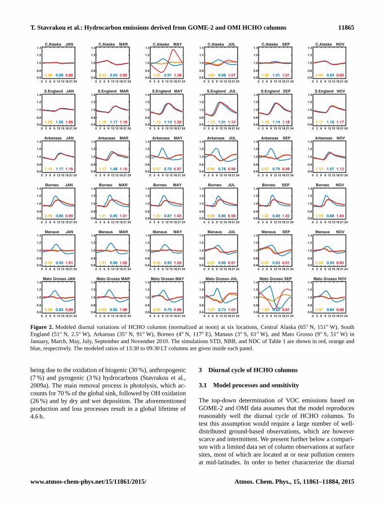
Figure 2. Modeled diurnal variations of HCHO columns (normalized at noon) at six locations, Central Alaska (65◦ N, 151◦W), South

England (51◦ N, 2.5◦W), Arkansas (35◦ N, 91◦W), Borneo (4◦ N, 117◦ E), Manaus (3◦ S, 61◦W), and Mato Grosso (9◦ S, 51◦W) in

January, March, May, July, September and November 2010. The simulations STD, NBB, and NDC of Table 1 are shown in red, orange and

blue, respectively. The modeled ratios of 13:30 to 09:30 LT columns are given inside each panel.

being due to the oxidation of biogenic (30 %), anthropogenic

(7 %) and pyrogenic (3 %) hydrocarbons (Stavrakou et al.,

2009a). The main removal process is photolysis, which ac-

counts for 70 % of the global sink, followed by OH oxidation

(26 %) and by dry and wet deposition. The aforementioned

production and loss processes result in a global lifetime of

4.6 h.

3 Diurnal cycle of HCHO columns

3.1 Model processes and sensitivity

The top-down determination of VOC emissions based on

GOME-2 and OMI data assumes that the model reproduces

reasonably well the diurnal cycle of HCHO columns. To

test this assumption would require a large number of well-

distributed ground-based observations, which are however

scarce and intermittent. We present further below a compari-

son with a limited data set of column observations at surface

sites, most of which are located at or near pollution centers

at mid-latitudes. In order to better characterize the diurnal



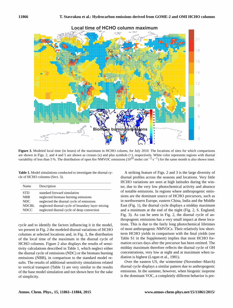
Local time of HCHO column maximum

Biomass burning emissions

Figure 3. Modeled local time (in hours) of the maximum in HCHO column, for July 2010. The locations of sites for which comparisons

are shown in Figs. 2, and 4 and 5 are shown as crosses (x) and plus symbols (+), respectively. White color represents regions with diurnal

variability of less than 5 %. The distribution of open fire NMVOC emissions (1010 molec cm−2 s−1) for the same month is also shown inset.

Table 1. Model simulations conducted to investigate the diurnal cy-

cle of HCHO columns (Sect. 3).

Name Description

STD standard forward simulation

NBB neglected biomass burning emissions

NDC neglected the diurnal cycle of emissions

NDCBL neglected diurnal cycle of boundary layer mixing

NDCC neglected diurnal cycle of deep convection

cycle and to identify the factors influencing it in the model,

we present in Fig. 2 the modeled diurnal variations of HCHO

columns at selected locations and, in Fig. 3, the distribution

of the local time of the maximum in the diurnal cycle of

HCHO columns. Figure 2 also displays the results of sensi-

tivity calculations described in Table 1, which neglect either

the diurnal cycle of emissions (NDC) or the biomass burning

emissions (NBB), in comparison to the standard model re-

sults. The results of additional sensitivity simulations related

to vertical transport (Table 1) are very similar to the results

of the base model simulation and not shown here for the sake

of simplicity.

A striking feature of Figs. 2 and 3 is the large diversity of

diurnal profiles across the seasons and locations. Very little

HCHO variations are seen at high latitudes during the win-

ter, due to the very low photochemical activity and absence

of notable emissions. In regions where anthropogenic emis-

sions are the dominant source of HCHO precursors, such as

in northwestern Europe, eastern China, India and the Middle

East (Fig. 1), the diurnal cycle displays a midday maximum

and a minimum at the end of the night (Fig. 2, S. England;

Fig. 3). As can be seen in Fig. 2, the diurnal cycle of an-

thropogenic emissions has a very small impact at these loca-

tions. This is due to the fairly long photochemical lifetimes

of most anthropogenic NMVOCs. Their relatively low short-

term HCHO yields in comparison with the final yields (see

Table S1 in the Supplement) implies that most HCHO for-

mation occurs days after the precursor has been emitted. The

midday maximum therefore reflects the diurnal cycle of OH

concentrations, very low at night and at maximum when ra-

diation is highest (Logan et al., 1981).

Over the eastern US, the wintertime (November–March)

diurnal cycle displays a similar pattern due to anthropogenic

emissions. In the summer, however, when biogenic isoprene

is the dominant VOC, a completely different behavior is pre-



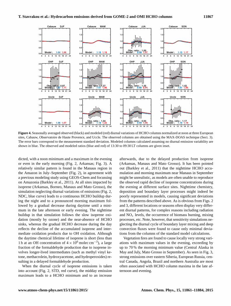
Figure 4. Seasonally averaged observed (black) and modeled (red) diurnal variations of HCHO columns normalized at noon at three European

sites, Cabauw, Observatoire de Haute Provence, and Uccle. The observed columns are obtained using the MAX-DOAS technique (Sect. 3).

The error bars correspond to the measurement standard deviation. Modeled columns calculated assuming no diurnal emission variability are

shown in blue. The observed and modeled ratios (blue and red) of 13:30 to 09:30 LT columns are given inset.

dicted, with a noon minimum and a maximum in the evening

or even in the early morning (Fig. 2, Arkansas; Fig. 3). A

relatively similar pattern is found in the Manaus region in

the Amazon in July–September (Fig. 2), in agreement with

a previous modeling study using GEOS-Chem and focussing

on Amazonia (Barkley et al., 2011). At all sites impacted by

isoprene (Arkansas, Borneo, Manaus and Mato Grosso), the

simulation neglecting diurnal variations of emissions (Fig. 2,

NDC, blue curve) leads to a continuous HCHO buildup dur-

ing the night and to a pronounced morning maximum fol-

lowed by a gradual decrease during daytime until a mini-

mum in the late afternoon or early evening. The nighttime

buildup in that simulation follows the slow isoprene oxi-

dation (mostly by ozone) and the near-absence of HCHO

sinks, whereas the gradual HCHO decrease during the day

reflects the decline of the accumulated isoprene and inter-

mediate oxidation products due to OH oxidation. Although

the daytime chemical lifetime of isoprene is short (less than

1 h at an OH concentration of 4× 106 molec cm−3), a large

fraction of the formaldehyde production due to isoprene in-

volves longer-lived intermediates (such as methyl vinyl ke-

tone, methacrolein, hydroxyacetone, and hydroperoxides) re-

sulting in a delayed formaldehyde production.

When the diurnal cycle of isoprene emissions is taken

into account (Fig. 2, STD, red curve), the midday emission

maximum leads to a HCHO minimum and to an increase

afterwards, due to the delayed production from isoprene

(Arkansas, Manaus and Mato Grosso). It has been pointed

out (Barkley et al., 2011) that the nighttime HCHO accu-

mulation and morning maximum near Manaus in September

might be unrealistic, as models are often unable to reproduce

the observed rapid decline of isoprene concentrations during

the evening at different surface sites. Nighttime chemistry,

deposition and boundary layer processes might indeed be

poorly represented in models, causing significant deviations

from the patterns described above. As is obvious from Figs. 2

and 3, different locations or seasons often display very differ-

ent diurnal patterns, for complex reasons including radiation

and NOx levels, the occurrence of biomass burning, mixing

processes, etc. Note, however, that sensitivity simulations ne-

glecting the diurnal cycle of boundary layer mixing and deep

convection fluxes were found to cause only minimal devia-

tions from the columns of the standard model calculations.

Vegetation fires are found to cause locally very strong vari-

ations with maximum values in the evening, exceeding by

up to 70 % the morning minimum value (Central Alaska in

May and July, Mato Grosso in September). As seen in Fig. 3,

strong emissions over eastern Siberia, European Russia, cen-

tral Canada, Angola, Brazil and northern Australia are most

often associated with HCHO column maxima in the late af-

ternoon and evening.



Beijing DJF

0 3 6 9 12 15 18 21 24

0.0

0.5

1.0

1.5

2.0

Obs. ratio : 1.11Model : 1.13 1.18

Beijing MAM

0 3 6 9 12 15 18 21 24

0.0

0.5

1.0

1.5

2.0

Obs. ratio : 0.84Model : 1.20 1.26

Beijing JJA

0 3 6 9 12 15 18 21 24

0.0

0.5

1.0

1.5

2.0

Obs. ratio : 1.17Model : 1.03 1.18

Beijing SON

0 3 6 9 12 15 18 21 24

0.0

0.5

1.0

1.5

2.0

Obs. ratio : 1.11Model : 1.20 1.26

Xianghe DJF

0 3 6 9 12 15 18 21 24

0.0

0.5

1.0

1.5

2.0

Obs. ratio : 1.06Model : 1.13 1.18

Xianghe MAM

0 3 6 9 12 15 18 21 24

0.0

0.5

1.0

1.5

2.0

Obs. ratio : 0.93Model : 1.20 1.26

Xianghe JJA

0 3 6 9 12 15 18 21 24

0.0

0.5

1.0

1.5

2.0

Obs. ratio : 1.14Model : 1.03 1.18

Xianghe SON

0 3 6 9 12 15 18 21 24

0.0

0.5

1.0

1.5

2.0

Obs. ratio : 1.18Model : 1.20 1.26

Bujumbura DJF

0 3 6 9 12 15 18 21 24

0.0

0.5

1.0

1.5

2.0

Obs. ratio : 0.79Model : 0.82 0.93

Bujumbura MAM

0 3 6 9 12 15 18 21 24

0.0

0.5

1.0

1.5

2.0

Obs. ratio : 0.56Model : 0.80 0.95

Bujumbura JJA

0 3 6 9 12 15 18 21 24

0.0

0.5

1.0

1.5

2.0

Model : 0.74 0.91

Bujumbura SON

0 3 6 9 12 15 18 21 24

0.0

0.5

1.0

1.5

2.0

Model : 0.79 0.93

Reunion DJF

0 3 6 9 12 15 18 21 24

0.0

0.5

1.0

1.5

2.0

Model : 1.04 1.04

Reunion MAM

0 3 6 9 12 15 18 21 24

0.0

0.5

1.0

1.5

2.0

Model : 1.07 1.07

Reunion JJA

0 3 6 9 12 15 18 21 24

0.0

0.5

1.0

1.5

2.0

Obs. ratio : 1.04Model : 1.10 1.10

Reunion SON

0 3 6 9 12 15 18 21 24

0.0

0.5

1.0

1.5

2.0

Obs. ratio : 1.14Model : 1.02 1.02

Figure 5. As in Fig. 4, comparison between modeled and observed diurnal variations for four sites : Beijing, Xianghe, Bujumbura and Re-

union Island. The observations were obtained using the MAX-DOAS (Beijing, Xianghe, Bujumbura) and FTIR (Reunion Island) techniques.

3.2 Model evaluation

To evaluate the diurnal cycle of the modeled HCHO column,

we use ground-based, remotely sensed measurements at the

seven following sites:

1. Cabauw, the Netherlands (52◦ N, 5◦ E), 8 June–21 July

2009 (Pinardi et al., 2013).

2. Observatoire de Haute Provence (OHP), France

(43.94◦ N, 5.71◦ E), 26 June 2007–20 March 2013

(Valks et al., 2011).

3. Uccle, Belgium (50.78◦ N, 4.35◦ E), 1 May 2011–

23 April 2012 (Gielen et al., 2014).

4. Beijing, China (39.98◦ N, 116.38◦ E), 3 July 2008–

17 April 2009 (Vlemmix et al., 2015, see also Hendrick

et al., 2014).

5. Xianghe, China (39.75◦ N, 116.96◦ E), 7 March 2010–

26 December 2013 (Vlemmix et al., 2015, see also Hen-

drick et al., 2014).

6. Bujumbura, Burundi (3◦ S, 29◦ E), 25 November 2013–

22 January 2014 (De Smedt et al., 2015).

7. Reunion Island, France (20.9◦ S, 55.5◦ E), 1 August

2004–25 October 2004, 21 May 2007–15 October 2007,

2 June 2009–28 December 2009, and 11 January 2010–

16 December 2010 (Vigouroux et al., 2009).

The MAX-DOAS (Multi-axis differential optical absorp-

tion spectroscopy) technique (Hönninger et al., 2004; Platt

and Stutz, 2008) was used in all cases, except at Reunion

Island where the FTIR (Fourier transform infrared spec-

troscopy) technique is used (Griffiths and de Haseth, 2007;

Vigouroux et al., 2009). Total HCHO columns are measured

at all stations, and profiles are also measured at Beijing, Xi-

anghe, and Bujumbura.

Figures 4 and 5 illustrate the diurnal cycle of observed and

modeled HCHO columns seasonally averaged and normal-

ized by their noon values. The ratio of the observed columns

at 13:30 and 09:30 LT ranges mostly between 0.8 and 1.2, al-

though values close to 1.4 are found at one site (OHP). The



modeled values of this ratio are most often higher than in

the measurements, except at OHP. The average ratio at all

sites and seasons is slightly higher in the model (1.126) than

in the data (1.043), although the average absolute deviation

between model and data is large (20 %), presumably mostly

because of representativity issues. The coarse resolution of

the model makes it impossible to reproduce the very large

differences seen, for example, between the observed diurnal

profiles at Beijing and Xianghe, two sites very near to each

other and within the same model grid cell. OHP similarly

lies in a region with strong gradients in the diurnal behavior

of the columns, as seen in Fig. 3.

Nevertheless, the diurnal cycle of HCHO columns at the

four most polluted sites (Uccle, Cabauw, Beijing and Xi-

anghe) shows a consistent pattern during summertime (also

in spring and fall at Uccle) which is well reproduced by the

model. Additionally, at Reunion Island, the observed midday

maximum is well reproduced by the model. As pointed out

above, the midday maximum at both very remote and very

polluted sites is primarily caused by the diurnal cycle of OH

levels, as the reaction with OH of the (mostly fairly long-

lived) anthropogenic VOCs as well as methane is the main

source of HCHO in those areas. In the Beijing area, the di-

urnal cycle of emissions is responsible for a slight delay in

the maximum towards the afternoon, in agreement with the

observations.

A broader network of measurements would be necessary

to provide a more detailed assessment of HCHO column di-

urnal variations, in particular over forests and in biomass

burning areas. Nevertheless, the comparison presented above

with the limited data set of available measurements revealed

no large systematic discrepancies, except for a slight overes-

timation (by 8 %) of the average ratio of 13:30 to 09:30 LT

columns.

4 Satellite observations

The current version (v14) of the HCHO retrievals applied to

GOME-2/Metop-A and OMI/Aura measurements is based

on the algorithm developed for GOME-2 (version 12, De

Smedt et al., 2012), with significant adaptations, as detailed

below.

A classical DOAS algorithm is used, including three main

steps: (1) the fit of absorption cross-section databases to the

measured Earth reflectance in order to retrieve HCHO slant

columns, (2) a background normalization procedure to elimi-

nate remaining unphysical dependencies, and (3) the calcula-

tion of tropospheric air mass factors using radiative transfer

calculations and modeled a priori profiles. In GOME-2 v12,

two fitting intervals were introduced to improve the treatment

of BrO absorption features, and to reduce the noise on the

HCHO columns (328.5–359 nm for the pre-fit of BrO, 328.5–

346 nm for the fit of HCHO) (De Smedt et al., 2012).

In the current version, a third fitting interval (339–364 nm)

is used to pre-fit the O2–O2 slant columns in order to mini-

mize the effect of spectral interferences between the molec-

ular absorptions. This results in a global reduction of the

HCHO slant columns over the continents compared to the

previous version, by 0–25 %, depending on the season and

the altitude. It is interesting to note that the effect is very sim-

ilar when applied to GOME-2 and OMI HCHO retrievals,

i.e., it has little or no impact on the diurnal variations (De

Smedt et al., 2015). In order to improve the fit of the slant

columns, an iterative DOAS algorithm for removal of spike

residuals has been implemented (Richter et al., 2011). In

addition, this version of the algorithm makes use of radi-

ance spectra, daily averaged in the equatorial Pacific, which

serve as reference spectra. The background normalization

now depends on the day, the latitude, and on the viewing

zenith angle of the observation. This also serves as a de-

striping procedure, needed for an imager instrument such as

OMI (Boersma et al., 2011). The air mass factor calcula-

tion is based on Palmer et al. (2001). Scattering weighting

functions are calculated with the LIDORT v3.3(linearized

discrete ordinate radiative transfer) radiative transfer model

(Spurr, 2008).

The a priori profile shapes are provided by the IMAGES

model, at 09:30 LT for GOME-2 and 13:30 LT for OMI (cf.

Sect. 2). The OMI-based surface reflection database from

Kleipool et al. (2008) is used for both GOME-2 and OMI.

Radiative cloud effects are corrected using the independent

pixel approximation (Martin et al., 2002) and the respective

cloud products of the instruments provided by the TEMIS

website (http://www.temis.nl), namely the GOME-2 O2 A-

band Frescov6 product (Wang et al., 2008) and the OMI O2–

O2 cloud product (Stammes et al., 2008). As for the previous

algorithm versions, v14 HCHO columns are openly available

on the TEMIS website (http://h2co.aeronomie.be/).

Monthly averaged HCHO columns from both instruments

gridded onto the resolution of the model are used as top-

down constraints. The simulated monthly averaged columns

are calculated from daily values weighted by the number of

satellite (OMI or GOME-2) measurements for each day at

each model grid cell. Columns with a cloud fraction higher

than 40 % are excluded from the averages. HCHO data are

also excluded over oceanic IMAGES grid cells (for which

the land fraction is lower than 0.2), since we aim to con-

strain only continental sources, as well as in the region of the

South Atlantic geomagnetic anomaly, i. e. within less than

1500 km of its assumed epicenter (47.0◦W, 24.9◦ S). Finally,

regridded columns for which the monthly and spatially av-

eraged retrieval error exceeds 100 % are also rejected. The

error of the satellite columns is defined as the square root of

the squared sum of the retrieval error and an absolute error

of 2×1015 molec cm−2. In most VOC-emitting regions the

error ranges between 40 and 60 %.

The monthly regridded HCHO columns from GOME-2

and OMI are shown in Fig. 6 for July 2010. As seen in this


http://www.temis.nl

http://h2co.aeronomie.be/


Figure 6. Observed (upper panels) HCHO columns by GOME-2

and OMI instruments in July 2010. Simulated HCHO columns us-

ing IMAGESv2 CTM at the overpass times of GOME-2 and OMI

(middle panels), and optimized modeled columns derived from the

inversions using GOME-2 data (left) and OMI columns (right). The

columns are expressed in 1015 molec cm−2.

figure, and discussed in De Smedt et al. (2015), the early af-

ternoon columns of OMI are higher than the mid-morning

values of GOME-2 at mid-latitudes, while the reverse is true

at most tropical locations, in qualitative agreement with the

ground-based measurements and modeling results (Figs. 4,

5).

5 Inversion methodology

The flux inversion technique consists in minimizing the mis-

match between the model predictions and a set of chemi-

cal observations by adjusting the a priori emission distribu-

tions 8i(x, t), where (x, t) denote the spatial (latitude, lon-

gitude) and temporal (year, month) variables, and i the dif-

ferent emission categories (biogenic, pyrogenic, and anthro-

pogenic). We express the optimized solution 8opt

i (x, t) as

8opt

i (x, t)=

m∑j=1

efj8i(x, t), (1)

where f = (fj ) is a vector of scaling factors (in log space)

multiplying the a priori emissions. This vector is determined

Table 2. Performed flux inversions.

Name Description

GOME-2 use GOME-2 data

OMI use OMI data

OMI-DE doubled a priori errors on the emission fluxes

OMI-HE halved a priori errors on the emission fluxes

OMI-CF use only OMI data with cloud fraction < 0.2

OMI-IS ignore isomerization of isoprene peroxy radicals

so as to minimize the scalar function J (also termed as cost

function)

J (f )=1

2

((H(f )− y)TE−1(H(f )− y)+f TB−1f

), (2)

which measures the discrepancy between the modeled

HCHO columns H(f ) and the observations y. In this ex-

pression T is the transpose of the matrix, E and B are the ma-

trices of errors on the observations y and on the variables f ,

respectively. The gradient of the cost function J with respect

to the input variables (∂J/∂f ) is calculated using the adjoint

of the model. A thorough description of the method and its

implementation in the IMAGESv2 CTM is given in Müller

and Stavrakou (2005) and Stavrakou et al. (2009b). The in-

version is performed at the model resolution (2◦× 2.5◦) us-

ing an iterative algorithm suitable for large-scale problems

(Gilbert and Lemaréchal, 1989).

The source inversions presented in Table 2 infer the emis-

sion rates of the three emission categories (anthropogenic,

biogenic and biomass burning) are adjusted per month

and are constrained by either GOME-2 or OMI HCHO

columns. On the global scale, ca. 63 000 flux parameters

are varied. The emission of a grid cell is not optimized

when its maximum a priori monthly value is lower than

1010 molec cm−2 s−1. The assumed error on the a priori an-

thropogenic emission by country is set equal to a factor of 1.5

and 2 for OECD (Organisation for Economic Co-operation

and Development) and other countries, respectively, to a fac-

tor of 2 for biogenic emissions and to a factor of 3 for fire

burning emissions (Stavrakou et al., 2009b).

The sensitivity studies (Table 2) aim at assessing the im-

pact of (i) the choice of a priori errors on the emission fluxes

(OMI-DE, OMI-HE), (ii) the cloud fraction filter applied to

the satellite data (OMI-CF), and (iii) the isomerization of iso-

prene peroxy radicals (OMI-IS). The annual a priori and top-

down fluxes of the two standard and the four sensitivity inver-

sions are summarized in Table 3. The a priori model columns

calculated at 09:30 and 13:30 LT are generally higher than

the GOME-2 or OMI HCHO column abundances (Fig. 6),

e.g., over Europe, southern China, the United States, Amazo-

nia and Northern Africa. They are, however, found to agree

generally well in terms of seasonality (Fig. 7).



Table 3. A priori and top-down VOC emissions (Tg yr−1) by region. The emission inversions are defined in Table 2. The regions are

defined as follows. North America: US and Canada, Southern America: Mexico, Central and South America, Northern (Southern) Africa:

north (south) of the Equator, Tropics: 25◦ S–25◦ N, Southeastern US: 25–38◦ N, 60–100◦W, Amazonia: 14◦ S–10◦ N, 45–80◦W, Indonesia:

10◦ S–6◦ N, 95–142.5◦ E, Indochina: 6–22◦ N, 97.5–110◦ E, Europe extends to the Urals (55◦ E), FSU=Former Soviet Union.

Biomass burning (TgVOC yr−1) A priori GOME-2 OMI OMI-DE OMI-HE OMI-CF OMI-IS

North America 5.3 3.6 3.3 5.3 2.9 4.6 3.2

Southern America 36.9 20.7 17.1 16.8 17.8 16.4 16.2

Amazonia 26.5 13.0 10.4 10.2 10.8 10.0 9.7

Northern Africa 14.9 8.6 8.8 8.8 9.2 9.7 8.1

Southern Africa 25.8 17.6 23.8 24.6 23.0 25.5 23.1

Indochina 6.2 4.6 5.3 5.6 4.7 5.6 5.0

Tropics 93.3 56.8 60.6 61.6 60.4 63.0 57.8

Extratropics 12.0 10.0 9.9 13.4 8.8 12.1 9.2

Global 105.4 67.0 70.5 74.9 69.1 75.1 67.1

Isoprene (Tg yr−1) A priori GOME-2 OMI OMI-DE OMI-HE OMI-CF OMI-IS

Europe (excl. FSU) 3.8 3.3 3.8 3.7 3.4 3.9 3.7

Europe 7.4 6.9 8.2 8.8 7.7 8.6 8.1

North America 34.7 26.5 29.9 28.0 31.9 30.4 28.6

Southeastern US 14.5 8.9 10.8 9.8 12.2 11.3 9.9

Southern America 149.5 142.1 121.2 115.9 128.9 125.6 114.0

Amazonia 99.4 92.5 73.7 69.1 80.6 77.2 67.9

Northern Africa 50.6 45.3 43.7 40.4 46.8 44.7 41.5

Southern Africa 31.0 31.3 31.5 32.8 31.0 34.2 30.7

Indonesia 11.6 10.3 11.1 10.5 11.4 10.6 10.9

Indochina 7.6 7.1 7.5 7.3 7.5 7.4 7.3

Tropics 314.8 291.1 272.3 261.9 286.2 281.3 260.2

Extratropics 48.3 39.4 44.7 44.1 45.8 46.4 43.3

Global 363.1 330.5 317.0 305.9 332.1 327.8 303.5

Anthropogenic (TgVOC yr−1) A priori GOME-2 OMI OMI-DE OMI-HE OMI-CF OMI-IS

Global 155.6 138.6 157.5 162.0 154.2 163.4 155.8

6 Overview of the results

Globally, the cost function is reduced by a factor of 2 af-

ter optimization, and its gradient is reduced by a factor of

ca. 103. In general, the consistency between the two inver-

sions is highest in tropical regions. At mid-latitudes, the

emission updates (i.e., the ratios of optimized to prior emis-

sions) are almost systematically higher in the OMI-based in-

version than in the GOME-2-based inversion. This reflects

ratios of 13:30 to 09:30 LT columns which are lower in the

model than suggested by the two satellite data sets.

Both GOME-2 and OMI inversions suggest a strong de-

crease in global biomass burning VOC emissions with re-

gard to the a priori GFEDv3 inventory, by 36 and 33 %,

respectively. This decrease is most pronounced in tropical

regions. In contrast, both the OMI and GOME-2 optimiza-

tions lead to enhanced emissions (by about 50 %) due to

the extensive fires which plagued European Russia in Au-

gust 2010 (Sect. 7.2) and to agricultural waste burning in the

North China Plain in June (Sect. 7.3). The fire burning esti-

mates from the two base inversions are generally quite con-

sistent, not only globally but also over large emitting regions

like Amazonia, southeastern Asia, and Africa. The sensitivity

studies provide global flux estimates which are close (within

7 %) to the standard top-down results using OMI.

The globally derived isoprene fluxes are reduced in both

standard inversions, by 9 % according to GOME-2 and by

13 % according to OMI, compared to the a priori estimate

of the MEGAN–ECMWF-v2 inventory (363.1 Tg yr−1, Ta-

ble 3). The overall consistency between the global estimates

is high for this emission category, despite some significant

differences at a regional scale (cf. next sections). The bio-

genic top-down fluxes derived from the sensitivity inversions

of Table 2 lie within 5 % of the OMI-based estimates on the

global scale, yet larger differences are found in the regional

scale.

Finally, the global anthropogenic source is decreased in

the GOME-2 inversion, while it is slightly increased in the

inversion using OMI. Despite their limited capability to con-

strain this emission category on the global scale due to its

small contribution to the global HCHO budget (Stavrakou

et al., 2009a), the satellite observations are found to provide



Northeastern US (38-46 N, 270-90 W)

j m m j s n0

5

10

15

20

1015

mo

lec.

cm

-2

GOME-2OMI

2.8 2.1 1.5 1.2

Southeastern US (26-42 N, 75-95 W)

j m m j s n0

5

10

15

20

25

1015

mo

lec.

cm

-2

GOME-2OMI

2.9 1.9 1.6 0.9

Southern China (18-34 N, 110-120 E)

j m m j s n0

5

10

15

20

1015

mo

lec.

cm

-2

GOME-2OMI

1.6 0.9 1.2 0.9

Indochina (10-18 N, 105-110 E)

j m m j s n0

5

10

15

20

25

1015

mo

lec.

cm

-2

GOME-2OMI

2.2 1.8 2.4 1.8

Congo (2-10 S, 15-30 E)

j m m j s n0

5

10

15

20

25

1015

mo

lec.

cm

-2

GOME-2OMI

1.0 0.7 1.0 0.3

Southern Africa (6-18 S, 10-30 E)

j m m j s n0

5

10

15

1015

mo

lec.

cm

-2

GOME-2OMI

1.6 0.6 1.1 0.5

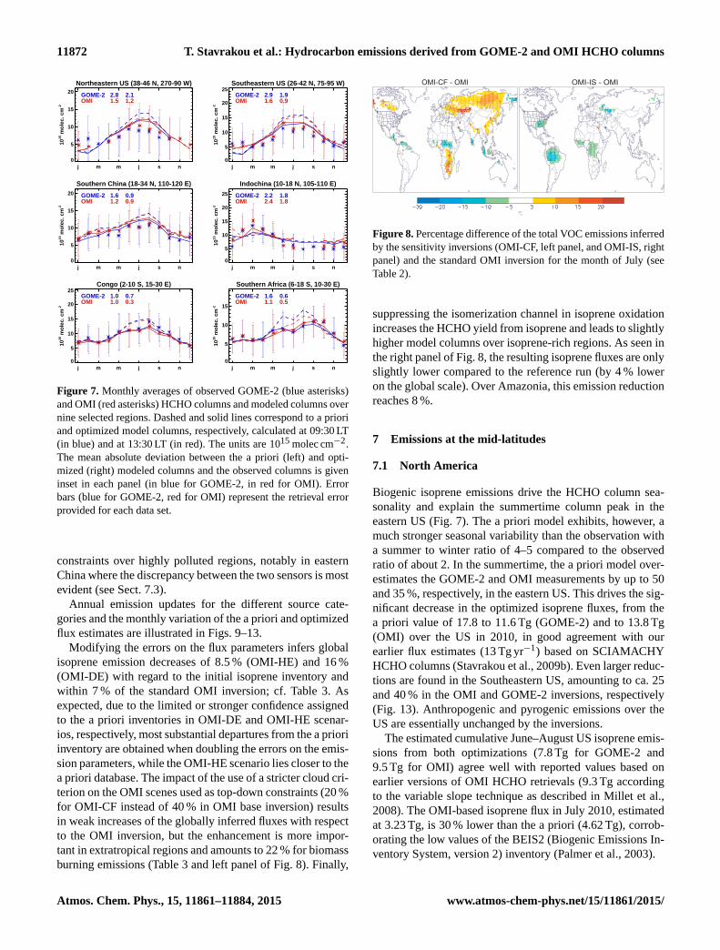
Figure 7. Monthly averages of observed GOME-2 (blue asterisks)

and OMI (red asterisks) HCHO columns and modeled columns over

nine selected regions. Dashed and solid lines correspond to a priori

and optimized model columns, respectively, calculated at 09:30 LT

(in blue) and at 13:30 LT (in red). The units are 1015 molec cm−2.

The mean absolute deviation between the a priori (left) and opti-

mized (right) modeled columns and the observed columns is given

inset in each panel (in blue for GOME-2, in red for OMI). Error

bars (blue for GOME-2, red for OMI) represent the retrieval error

provided for each data set.

constraints over highly polluted regions, notably in eastern

China where the discrepancy between the two sensors is most

evident (see Sect. 7.3).

Annual emission updates for the different source cate-

gories and the monthly variation of the a priori and optimized

flux estimates are illustrated in Figs. 9–13.

Modifying the errors on the flux parameters infers global

isoprene emission decreases of 8.5 % (OMI-HE) and 16 %

(OMI-DE) with regard to the initial isoprene inventory and

within 7 % of the standard OMI inversion; cf. Table 3. As

expected, due to the limited or stronger confidence assigned

to the a priori inventories in OMI-DE and OMI-HE scenar-

ios, respectively, most substantial departures from the a priori

inventory are obtained when doubling the errors on the emis-

sion parameters, while the OMI-HE scenario lies closer to the

a priori database. The impact of the use of a stricter cloud cri-

terion on the OMI scenes used as top-down constraints (20 %

for OMI-CF instead of 40 % in OMI base inversion) results

in weak increases of the globally inferred fluxes with respect

to the OMI inversion, but the enhancement is more impor-

tant in extratropical regions and amounts to 22 % for biomass

burning emissions (Table 3 and left panel of Fig. 8). Finally,

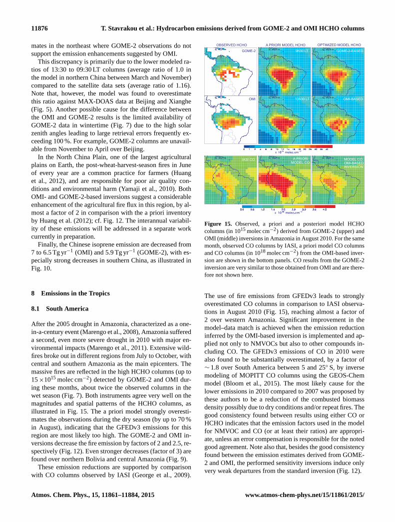
OMI-CF - OMI OMI-IS - OMI

Figure 8. Percentage difference of the total VOC emissions inferred

by the sensitivity inversions (OMI-CF, left panel, and OMI-IS, right

panel) and the standard OMI inversion for the month of July (see

Table 2).

suppressing the isomerization channel in isoprene oxidation

increases the HCHO yield from isoprene and leads to slightly

higher model columns over isoprene-rich regions. As seen in

the right panel of Fig. 8, the resulting isoprene fluxes are only

slightly lower compared to the reference run (by 4 % lower

on the global scale). Over Amazonia, this emission reduction

reaches 8 %.

7 Emissions at the mid-latitudes

7.1 North America

Biogenic isoprene emissions drive the HCHO column sea-

sonality and explain the summertime column peak in the

eastern US (Fig. 7). The a priori model exhibits, however, a

much stronger seasonal variability than the observation with

a summer to winter ratio of 4–5 compared to the observed

ratio of about 2. In the summertime, the a priori model over-

estimates the GOME-2 and OMI measurements by up to 50

and 35 %, respectively, in the eastern US. This drives the sig-

nificant decrease in the optimized isoprene fluxes, from the

a priori value of 17.8 to 11.6 Tg (GOME-2) and to 13.8 Tg

(OMI) over the US in 2010, in good agreement with our

earlier flux estimates (13 Tg yr−1) based on SCIAMACHY

HCHO columns (Stavrakou et al., 2009b). Even larger reduc-

tions are found in the Southeastern US, amounting to ca. 25

and 40 % in the OMI and GOME-2 inversions, respectively

(Fig. 13). Anthropogenic and pyrogenic emissions over the

US are essentially unchanged by the inversions.

The estimated cumulative June–August US isoprene emis-

sions from both optimizations (7.8 Tg for GOME-2 and

9.5 Tg for OMI) agree well with reported values based on

earlier versions of OMI HCHO retrievals (9.3 Tg according

to the variable slope technique as described in Millet et al.,

2008). The OMI-based isoprene flux in July 2010, estimated

at 3.23 Tg, is 30 % lower than the a priori (4.62 Tg), corrob-

orating the low values of the BEIS2 (Biogenic Emissions In-

ventory System, version 2) inventory (Palmer et al., 2003).



GOME-2-based biomass burning emission update

OMI-based biomass burning emission update

JANUARY

JANUARY

MARCH

MARCH

AUGUST

AUGUST

OCTOBER

OCTOBER

Figure 9. Ratios of optimized to a priori pyrogenic VOC fluxes derived by source inversion of HCHO columns from GOME-2 (upper panels)

and OMI (lower panels) in January, March, August and October 2010. Ratio values between 0.9 and 1.1 are not shown for the sake of clarity.

GOME-2-based isoprene emission update

OMI-based isoprene emission update

JANUARY JULY

JULYJANUARY

Figure 10. Same as Fig. 9, but for isoprene emissions in January

and July.

The model predictions are compared to HCHO measure-

ments from the INTEX-A aircraft campaign conducted in

July–August 2004 over the eastern US (Singh et al., 2006;

Fried et al., 2008), shown in Fig. 14. It is worth noting that the

measurements by NCAR (National Center for Atmospheric

Research) and URI (Univ. Rhode Island) exhibit large differ-

ences between them, the NCAR values being ca. 50 % higher

than URI values below 2 km altitude (Fig. 14). The model

simulations are performed for 2004, and the concentrations

are sampled at the locations and times of the airborne mea-

Anthropogenic VOC emission update

GOME-2-based OMI-based

Figure 11. Same as Fig. 9, but for annual anthropogenic VOC

fluxes.

surements. In the a posteriori simulation shown in Fig. 14,

the bottom-up isoprene emissions for 2004 were multiplied

by the isoprene emission update inferred from either the OMI

or the GOME-2 inversion for 2010. As seen in Fig. 14, the av-

erage HCHO concentration below 2 km altitude decreased by

about 10 % in the OMI inversion (15 % in the case of GOME-

2) and remains within the range of the NCAR and URI mea-

surements. Despite the marked underestimation of the mod-

eled HCHO (1.39 and 1.32 ppbv in the OMI and GOME-2 in-

versions) in comparison to NCAR observations (1.83 ppbv),

the emission optimization results in an increased Pearson’s

spatial correlation coefficient between the modeled and ob-

served concentrations below 2 km, from 0.74 in the a priori to

0.79 and 0.80 in the OMI and GOME-2 inversions. A similar

improvement is found with respect to URI data.

7.2 Russia

The a priori model underpredicts the observed OMI HCHO

columns during the Russian fires of July–August 2010 by up

to a factor of 2, in particular over a broad region extending to



Global

j m m j s n

0

5

10

15

20

25

A priori

GOME-2

OMI

OMI-DE

OMI-HE

105.3

67.0

70.5

74.9

69.1

Amazonia

j m m j s n

0

5

10

15 A priori

GOME-2

OMI

OMI-DE

OMI-HE

26.5

13.0

10.4

10.2

10.8

Northern Africa

j m m j s n

0

1

2

3

4

5

6 A priori

GOME-2

OMI

OMI-DE

OMI-HE

14.9

8.6

8.8

8.8

9.2

Southern Africa

j m m j s n

0

2

4

6

A priori

GOME-2

OMI

OMI-DE

OMI-HE

25.8

17.6

23.8

24.6

23.0

Indochina

j m m j s n

0

1

2

3

4A priori

GOME-2

OMI

OMI-DE

OMI-HE

6.2

4.6

5.3

5.6

4.7

Europe

j m m j s n

0.0

0.2

0.4

0.6

0.8A priori

GOME-2

OMI

OMI-DE

OMI-HE

1.0

1.2

1.4

1.5

1.2

China

j m m j s n

0.0

0.2

0.4

0.6

0.8 A priori

GOME-2

OMI

OMI-DE

OMI-HE

1.8

2.0

2.4

2.7

2.1

N. America

j m m j s n

0.0

0.5

1.0

1.5

2.0

A priori

GOME-2

OMI

OMI-DE

OMI-HE

5.3

3.6

3.3

5.3

2.9

Figure 12. Monthly variation of a priori and top-down biomass burning VOC fluxes for Amazonia (14◦ S–10◦ N, 45–80◦W), Africa north

and south of the Equator, Indochina (6–22◦ N, 97.5–110◦ E), Europe (including European Russia), N. America (US and Canada), China, and

worldwide, expressed in teragrams of VOCs per month. Solid lines are used for the a priori emissions (black), and updated emissions inferred

from GOME-2 (blue) and OMI (red) observations. Dotted and dashed red lines are used for the results of the sensitivity studies OMI-DE and

OMI-HE (Table 2), respectively. For each inversion, annual fluxes for 2010 (in TgVOC) are given inside the panels.

Global

j m m j s n

0

10

20

30

40

50A prioriGOME-2OMIOMI-DEOMI-HE

363.1330.5317.0305.9332.1

Amazonia

j m m j s n

0

5

10

15 A prioriGOME-2OMIOMI-DEOMI-HE

99.492.573.769.180.6

Northern Africa

j m m j s n

0

2

4

6

A prioriGOME-2OMIOMI-DEOMI-HE

50.645.343.740.446.8

Southern Africa

j m m j s n

0

1

2

3

4

5


31.031.331.532.831.0

Indonesia

j m m j s n

0.0

0.5

1.0

1.5A prioriGOME-2OMIOMI-DEOMI-HE

11.610.311.110.511.4

Europe

j m m j s n

0

1

2

3


7.46.98.28.87.8

US

j m m j s n

0

1

2

3

4

5A prioriGOME-2OMIOMI-DEOMI-HE

17.811.613.812.615.4

Southeastern US

j m m j s n

0

1

2

3

A prioriGOME-2OMIOMI-DEOMI-HE

14.58.910.89.812.2

Figure 13. Monthly variation of a priori and satellite-derived isoprene fluxes for Amazonia, Northern and Southern Africa, Europe, N.

America (defined as in Fig. 12), Indonesia (10◦ S–6◦ N, 95–142.5◦ E), and the Southeastern US (25–38◦ N, 60–100◦W). The color and line

code is the same as in Fig. 12. Units are teragrams of isoprene per month. Annual isoprene fluxes per region are given in each panel in

teragrams of isoprene.

the north (61◦ N) and east (55◦ E) of Moscow (Fig. 6, upper

panel). Similar spatial patterns are also observed in GOME-2

HCHO columns. However, the GOME-2 columns are lower

than OMI over this region, and the model underestimation is

less severe, in this case reaching 60 %. The lower GOME-

2 values might be due to the lower retrieval sensitivity of

GOME-2 to lower tropospheric HCHO compared to OMI

at these latitudes, associated with larger solar zenith angles



1.83 ppbv

1.54 ppbv 1.39 ppbv

1.23 ppbv

Figure 14. Comparison between HCHO measurements from the

INTEX-A campaign and model concentrations sampled at the mea-

surement times and locations from the a priori simulation and from

the OMI-based inversion averaged between the surface and 2 km.

The HCHO data are reported from two different instruments, from

the National Center for Atmospheric Research (NCAR) and from

the University of Rhode Island (URI). The observed and modeled

mean HCHO concentrations over the flight domain and altitude

range are given inside each panel.

(De Smedt et al., 2015). As a result, the increase of the py-

rogenic emission fluxes is strongest in the OMI inversion,

from 440 GgVOC in the GFEDv3 inventory to 720 GgVOC

(630 GgVOC in GOME-2) in August 2010 over Europe. Ac-

cordingly, the isoprene fluxes inferred from the OMI in-

version in August are also larger, about 40 % higher than

the a priori estimate in the Moscow area, whereas the in-

crease derived by GOME-2 does not exceed 25 %. Overall,

the OMI data suggest annual isoprene fluxes in Europe are

11 % higher than the a priori inventory (Table 3). Note that,

although the isoprene enhancement over Russia peaks ear-

lier (July) and at slightly higher latitudes (ca. 61◦ N) than the

biomass burning emission enhancement (55–57◦ N in Au-

gust), the significant overlap of the two distributions makes it

impossible to rule out that pyrogenic emissions are the only

cause for the observed strong formaldehyde columns. The

very widespread extent of the observed formaldehyde plume

cannot be easily explained by the comparatively much more

localized emissions of the GFEDv3 inventory, and an addi-

tional, more widespread formaldehyde source (such as iso-

prene) could help to explain the observations. However, as

discussed below, the GFEDv3 total emissions over Russia

are likely largely underestimated, and their geographical dis-

tribution might also be in error. It is therefore possible that

these fires were more widespread than in GFEDv3 and that

strong isoprene emission enhancements are not needed to ex-

plain the observations.

Strongly enhanced fire emissions in the Moscow region

between mid-July and mid-August 2010 were reported based

on satellite observations of CO from MOPITT (Measure-

ments Of Pollution In The Troposphere; Konovalov et al.,

2011) and IASI (Krol et al., 2013; R’honi et al., 2013) and

on surface measurements (Konovalov et al., 2011). The op-

timized fire emission inferred by assimilation of IASI CO

columns in Krol et al. (2013) lies within 22 and 27 Tg CO

during the fires, i.e., about 7–10 times higher than in the

bottom-up inventory (GFEDv3). These values are compara-

ble with the ranges of 19–33 and 34–40 Tg CO suggested by

R’honi et al. (2013) and Yurganov et al. (2011), respectively,

but are much higher than reported values of ca. 10 Tg CO de-

rived using surface CO measurements in the Moscow area

(Konovalov et al., 2011). The latter study identifies the con-

tribution of peat burning to the total CO fire emission in this

region to be as high as 30 %.

The IMAGESv2 a priori CO simulation (using GFEDv3

inventory) underestimates substantially the IASI CO obser-

vations. Scaling the CO emissions in IMAGESv2 to the fire

VOC increase suggested by the OMI HCHO optimization,

i.e., ca. 60 % in July and August 2010, barely improves the

model agreement with the satellite, indicating that, in accor-

dance with earlier studies, more drastic fire flux enhance-

ments (factor of 5–10) are required to reconcile CO model-

data mismatches. The reasons for the differences in the emis-

sion increases inferred by CO and HCHO during the 2010

Russian fires are currently unknown, but they could be re-

lated either to inadequate knowledge of emission factors of

CO and VOCs from peat fires and/or underestimated re-

motely sensed HCHO columns over fire scenes due to pos-

sibly important aerosol effects not accounted for in the re-

trievals.

7.3 China

The dominant emission source in China is anthropogenic and

is estimated at 25.5 TgVOC in REASv2 (Kurokawa et al.,

2013) for 2008. The biogenic source, mainly located in

southern China, amounts to 7 Tg in 2010 in the MEGAN–

MOHYCAN-v2 inventory (Stavrakou et al., 2014; Guenther

et al., 2006, 2012). In northern China, the HCHO columns

are underestimated by the a priori model in winter compared

to OMI, whereas a relatively good agreement is found in

summer. In southern China, a general model overestimation

is found all year round (Figs. 6, 7).

Although the OMI-based inversion yields total Chi-

nese anthropogenic emissions very similar to the a pri-

ori (24.6 TgVOC), the emission patterns are modified with

increased emissions in northeastern China and especially

around Beijing (20–40 %) and emission reductions in the

southeast and in particular around Shanghai (15–47 %) and

Guangzhou (15–30 %). The total GOME-2 emission, esti-

mated at 20.6 TgVOC, is lower than the OMI result but

in good agreement with the estimate (20.2 Tg in 2008) of

the Multi-resolution Emission Inventory for China (MEIC,

http://www.meicmodel.org). The flux distributions from both

inversions have common features, e.g., decreased fluxes in

Shanghai and Guangzhou regions, but contradicting esti-


http://www.meicmodel.org


mates in the northeast where GOME-2 observations do not

support the emission enhancements suggested by OMI.

This discrepancy is primarily due to the lower modeled ra-

tios of 13:30 to 09:30 LT columns (average ratio of 1.0 in

the model in northern China between March and November)

compared to the satellite data sets (average ratio of 1.16).

Note that, however, the model was found to overestimate

this ratio against MAX-DOAS data at Beijing and Xianghe

(Fig. 5). Another possible cause for the difference between

the OMI and GOME-2 results is the limited availability of

GOME-2 data in wintertime (Fig. 7) due to the high solar

zenith angles leading to large retrieval errors frequently ex-

ceeding 100 %. For example, GOME-2 columns are unavail-

able from November to April over Beijing.

In the North China Plain, one of the largest agricultural

plains on Earth, the post-wheat-harvest-season fires in June

of every year are a common practice for farmers (Huang

et al., 2012), and are responsible for poor air quality con-

ditions and environmental harm (Yamaji et al., 2010). Both

OMI- and GOME-2-based inversions suggest a considerable

enhancement of the agricultural fire flux in this region, by al-

most a factor of 2 in comparison with the a priori inventory

by Huang et al. (2012); cf. Fig. 12. The interannual variabil-

ity of these emissions will be addressed in a separate work

currently in preparation.

Finally, the Chinese isoprene emission are decreased from

7 to 6.5 Tg yr−1 (OMI) and 5.9 Tg yr−1 (GOME-2), with es-

pecially strong decreases in southern China, as illustrated in

Fig. 10.

8 Emissions in the Tropics

8.1 South America

After the 2005 drought in Amazonia, characterized as a one-

in-a-century event (Marengo et al., 2008), Amazonia suffered

a second, even more severe drought in 2010 with major en-

vironmental impacts (Marengo et al., 2011). Extensive wild-

fires broke out in different regions from July to October, with

central and southern Amazonia as the main epicenters. The

massive fires are reflected in the high HCHO columns (up to

15×1015 molec cm−2) detected by GOME-2 and OMI dur-

ing these months, about twice the observed columns in the

wet season (Fig. 7). Both instruments agree very well on the

magnitudes and spatial patterns of the HCHO columns, as

illustrated in Fig. 15. The a priori model strongly overesti-

mates the observations during the dry season (by up to 70 %

in August), indicating that the GFEDv3 emissions for this

region are most likely too high. The GOME-2 and OMI in-

versions decrease the fire emission by factors of 2 and 2.5, re-

spectively (Fig. 12). Even stronger decreases (factor of 3) are

found over northern Bolivia and central Amazonia (Fig. 9).

These emission reductions are supported by comparison

with CO columns observed by IASI (George et al., 2009).

GOME-2

OMI

OPTIMIZED MODEL HCHO

A PRIORI

MODEL CO

A PRIORI MODEL HCHO

13h30 LT OMI-BASED

IASI CO MODEL CO

OMI-BASED

INVERSION

9h30 LT GOME-2-BASED

OBSERVED HCHO

Figure 15. Observed, a priori and a posteriori model HCHO

columns (in 1015 molec cm−2) derived from GOME-2 (upper) and

OMI (middle) inversions in Amazonia in August 2010. For the same

month, observed CO columns by IASI, a priori model CO columns

and CO columns (in 1018 molec cm−2) from the OMI-based inver-

sion are shown in the bottom panels. CO results from the GOME-2

inversion are very similar to those obtained from OMI and are there-

fore not shown here.

The use of fire emissions from GFEDv3 leads to strongly

overestimated CO columns in comparison to IASI observa-

tions in August 2010 (Fig. 15), reaching almost a factor of

2 over western Amazonia. Significant improvement in the

model–data match is achieved when the emission reduction

inferred by the OMI-based inversion is implemented and ap-

plied not only to NMVOCs but also to other compounds in-

cluding CO. The GFEDv3 emissions of CO in 2010 were

also found to be substantially overestimated, by a factor of

∼ 1.8 over South America between 5 and 25◦ S, by inverse

modeling of MOPITT CO columns using the GEOS-Chem

model (Bloom et al., 2015). The most likely cause for the

lower emissions in 2010 compared to 2007 was proposed by

these authors to be a reduction of the combusted biomass

density possibly due to dry conditions and/or repeat fires. The

good consistency found between results using either CO or

HCHO indicates that the emission factors used in the model

for NMVOC and CO (or at least their ratios) are appropri-

ate, unless an error compensation is responsible for the noted

good agreement. Note also that, besides the good consistency

found between the emission estimates derived from GOME-

2 and OMI, the performed sensitivity inversions induce only

very weak departures from the standard inversion (Fig. 12).



Isoprene fluxes over Amazonia derived by GOME-2 and

OMI inversions are equal to 92.5 and 73.7 Tg, respectively.

These re 25 and 7 % lower than the prior and in good agree-

ment with previous studies using satellite HCHO observa-

tions from the SCIAMACHY instrument (Stavrakou et al.,

2009b). The seasonal variation of the posterior fluxes is con-

sistent with the a priori inventory, except during the tran-

sitional wet-to-dry period (April–June) with both GOME-2

and OMI satellite data sets pointing to a significant flux de-

crease of ca. 25 % (Fig. 13). This behavior confirms previ-

ous comparisons using GOME HCHO observations suggest-

ing that factors other than the temperature influence the ob-

served variability (Barkley et al., 2008), such as the growth

of new leaves causing a temporary shutdown of the emissions

(Barkley et al., 2009).

8.2 Indonesia

Fire activity was exceptionally low in 2010, with annual

emissions of about 0.1 TgVOC, i.e., about 2 orders of mag-

nitude less than for high years such as 2006 according to

GFEDv3.

The GOME-2- and OMI-inferred isoprene estimates show

good consistency over Indonesia all year round, amounting

to 10.3 and 11.1 Tg, respectively, and close to the a priori es-

timate (11.6 Tg). The inferred isoprene emissions are, how-

ever, half of the reported fluxes of 25 Tg yr−1 based on SCIA-

MACHY HCHO observations, which also decreased with re-

spect to their a priori isoprene flux of 35 Tg yr−1 (Stavrakou

et al., 2009b). In comparison to that study, the isoprene a

priori emissions used in the present work are strongly re-

duced over this region, due to a drastic reduction by a fac-

tor of 4.1 of the MEGANv2.1 basal isoprene rate for tropical

rainforests over Asia, as suggested by field measurements in

Borneo (Langford et al., 2010). This reduction implemented

in the MEGAN–MOHYCAN-v2 model (Stavrakou et al.,

2014) is found here to be corroborated by GOME-2 and OMI

HCHO measurements.

8.3 Indochina

The northern part of the Indochina Peninsula (primarily

Myanmar, also Assam in India and parts of Thailand) faces

intense forest fires during the dry season, as very well seen in

the GOME-2 and OMI HCHO time series, with values reach-

ing 15×1015 molec cm−2 in March, about 3 times higher

than in the wet season (Fig. 7).

Both the GOME-2 and OMI data point to substantial but

very contrasting updates in the pyrogenic fluxes during the

fire season (March, Fig. 9): flux reductions by a factor of

2–5 over Myanmar and surrounding forested areas, and flux

increases by a factor of almost 2 (or more in the case of

OMI) over the southeastern part of the peninsula, which in-

cludes Cambodia, southern Laos and southern Vietnam. In

the OMI-DE inversion assuming doubled errors on the a pri-

OBSERVED HCHO A PRIORI MODEL HCHO OPTIMIZED MODEL HCHO

GOME-2

OMI

9h30 LT GOME-2-BASED

OMI-BASED

IASI CO

A PRIORI

MODEL CO

MODEL CO

OMI-BASED

INVERSION

13h30 LT

Figure 16. Same as Fig. 15, for the Indochinese Peninsula in

March 2010.

ori fluxes, the updates are even more pronounced and reach

a factor of 4 over parts of Vietnam and Laos. The annual

emissions in the entire region are decreased by 15 and 26 %

according to the OMI and GOME-2 inversions, respectively.

As illustrated in Fig. 16, the optimization leads to a sub-

stantial improvement of the model performance, although the

HCHO columns remain significantly underestimated (by up

to 20 %) in the southern part of the peninsula (e.g., Cambo-

dia), most likely due to a too strong underestimation of the

GFEDv3 emissions used as a priori in the model. The emis-

sion drop over Myanmar and the need for higher emissions in

the southeast are partly confirmed by comparisons with IASI

CO columns. Indeed, as seen in the lower panel of Fig. 16,

modeled CO simulations using biomass burning fluxes opti-

mized using OMI data (i.e., reduced by ca. 26 % in March

relative to GFEDv3) display a better agreement with the ob-

served CO columns, despite an underestimation by ∼ 10 %

over most of the peninsula. This result is consistent with the

moderate reduction (ca. 20 % in March) of biomass burning

emissions of CO over tropical Asia inferred by Basu et al.

(2014) in an inversion based on IASI CO columns utiliz-

ing the TM5 (Transport Model 5) atmospheric model with

GFEDv3 as a priori inventory.

The strong enhancement of pyrogenic emissions required

to comply to the satellite data over the southeastern part of In-

dochina might be due to the occurrence of agricultural fires in

those regions (e.g., Cambodia), known to be a common man-

agement practice (Chang and Song, 2010). These fires are

very difficult to detect by satellite due to their limited spatial

extent. It is worth noting that the latest version of the Fire

Inventory from NCAR (FINNv1.5; Wiedinmyer et al., 2011)



predicts much higher emissions from this region: ca. 43 TgC

in March in the region 100–108◦ E, 10–18◦ N, i.e., a factor of

10 higher than in the GFEDv3 inventory (4.3 TgC). The dif-

ferences between GFEDv3 and FINN are most likely due to

inherent differences in the proxy variables used in the respec-

tive emission models, burned area in the case of GFEDv3,

and active fire counts in the FINN model, both retrieved

from MODIS satellite data. The two inventories provide,

however, very similar estimates for the more forested, north-

western part of Indochina (19–27◦ N, 97–100◦ E): 105 TgC

in GFEDv3, 124 TgC in FINNv1.5.

Considerable cloudiness during the rainy season (May–

October) causes gaps in the OMI HCHO time series, due

to the exclusion of scenes with ≥ 40 % cloud cover. The

GOME-2 data series are comparatively less affected by this

issue, due to the diurnal precipitation and cloudiness patterns

during the monsoon season. Indeed, long-term observations

over Indochina (Takahashi et al., 2010) reveal an early after-

noon rainfall peak (13:00–16:00 LT) and a heavy rainfall in

the early morning (04:00–07:00 LT) but lower precipitation

rates between 07:00 and 10:00 LT. GOME-2 observations are

therefore less contaminated by clouds and offer a better spa-

tial coverage during the rainy season in this region.

8.4 Africa

Over Africa, the annual pyrogenic source, amounting to

40.7 TgVOC in the a priori, is reduced to 26.2 and

32.6 TgVOC in the GOME-2 and OMI inversions, respec-

tively (Table 3). A smaller reduction is also inferred for iso-

prene fluxes, estimated at 76.6 Tg (GOME-2) and 75.2 Tg

(OMI), within 10 % of the a priori value (81.6 Tg). These es-

timates are in line with recently reported isoprene fluxes over

Africa based on the NASA data set of OMI HCHO columns

(77 TgC or 87 Tg isoprene compared to 116 Tg isoprene in

the a priori reported fluxes, Marais et al., 2012). The spatial

distribution of the emission updates is displayed in Figs. 9,

10 and 11.

African fire occurrence peaks in central Africa (e.g., the

Democratic Republic of the Congo or DRC) in early June

(Fig. 7) and lasts until August with the end of the dry sea-

son. The GOME-2 and OMI observations show an excel-

lent accordance, with morning columns being about 10 %

higher than in the afternoon, consistent with measurements

in Bujumbura (Fig. 5), although the morning to afternoon

ratio was found to be higher in the ground-based obser-

vations (1.25). The model simulations overpredict the ob-

servations of both sounders during the fire season by 10–

25 %. The posterior bias reduction (cf. Fig. 7, DRC region)

is achieved by a significant biomass burning flux decrease,

reaching a factor of 2 in the southern part of DRC, and 20–

30 % elsewhere between 2 and 12◦ S. In a similar manner,

up to a factor of 2 in emissions decrease is also needed in

the region of the central African republic during the fire sea-

son (November–February) to match the observed columns

(Fig. 7), in good agreement with our previous study using

SCIAMACHY HCHO columns (Stavrakou et al., 2009b).

Only small changes are inferred for isoprene emissions in

Northern Africa, with 11 % (GOME-2) and 16 % (OMI) de-

crease compared to the a priori emissions, as illustrated in

Fig. 13.

In Southern Africa, biogenic fluxes are highest in January

and lowest in July, while the fire season starts in May and

peaks in September (Figs. 12 and 13). Both GOME-2 and

OMI inversions infer only small isoprene flux updates (Ta-

ble 3). Regarding fire emissions, in contrast with GOME-

2 data suggesting a ca. 30 % flux reduction (to 17.6 from

25.8 TgVOC), the OMI-based estimate lies within 10 % of

the a priori, due to a compensation of flux decreases north of

approximately 15◦ S, and flux increases in the southernmost

part of the continent, south of ca. 15◦ S (Fig. 9). Although the

seasonal patterns are essentially preserved by the optimiza-

tion, both inversions predict higher emissions at the end of

the dry season, especially over Zambia and surrounding re-

gions (October; Figs. 9, 12). These updates are highest (fac-

tor of ∼ 2) in the OMI optimization, but the patterns are very

similar in both inversions.

9 Conclusions

The emissions of NMVOCs in 2010 were optimized by in-

verse modeling using the IMAGESv2 CTM and its adjoint

with HCHO column abundances from either GOME-2 or

OMI as observational constraint. Given their different over-

pass times, the consistency of the inferred emissions depends

on how the model can faithfully reproduce the diurnal cy-

cle of HCHO columns. The modeled diurnal cycle displays a

great variability mirroring the competing influences of pho-

tochemical productions and losses as well as the diurnal pro-

files of emissions and (to a lesser extent) meteorological pa-

rameters. Where anthropogenic VOCs are dominant, day-

time photochemical production and the anthropogenic emis-

sion profile lead to an early afternoon maximum, in agree-

ment with MAX-DOAS observations in Belgium, Holland

and (during summertime) the Beijing area. Over oceanic ar-

eas, where methane oxidation is the only significant source

in the model, a similar behavior is also simulated, in agree-

ment with FTIR data at Reunion Island. The poor model

performance at several locations (Bujumbura, OHP, Beijing

in winter/spring) is likely at least partly due to the coarse

model resolution, as shown by the very different diurnal pro-

files observed at Beijing and Xianghe. This limited repre-

sentativity of local ground-based sites possibly explains (part

of) the large deviations (typically±10–30 %) found between

the calculated and observed ratios of the HCHO columns at

13:30 and 09:30 LT. Despite this large scatter, the average ra-

tio of 13:30 LT columns to 09:30 LT columns is only slightly

higher (1.126) in the model compared to the MAX-DOAS

and FTIR measurements (1.043).



Unfortunately, no ground-based measurements are avail-

able in regions where the simulated diurnal cycle amplitude

is largest, namely over intense fire scenes at both tropical and

boreal latitudes. Over these regions, an evening maximum is

predicted, and the peak to trough ratio reaches up to 70 %. In

isoprene-rich areas, the diurnal HCHO cycle often, but not

always, displays a minimum around noon, when the photo-

chemical sink is highest, and a maximum in the late evening

or early morning, in agreement with a previous modeling

study (Barkley et al., 2011). Validation studies over forested

areas will be needed to determine how realistic these patterns

are.

The ratio of 13:30 to 09:30 LT columns is most often be-

tween 0.8 and 1.2 according to ground-based measurements.

Similar but generally higher values of this ratio are calcu-

lated by the model, 8 % higher on average. The satellite, on

the other hand, although in qualitative agreement with the

above, suggests higher ratios of 13:30 to 09:30 LT columns

than the model at mid-latitudes, whereas no clear pattern

emerges in tropical regions (Fig. 7). Nevertheless, these dis-

crepancies in terms of morning/afternoon ratios are most of-

ten small in comparison with the model–data differences in

the HCHO columns themselves. As a consequence, the emis-

sion fluxes inferred from both GOME-2 and OMI inversions

are found to be generally very consistent. They both suggest

a strong decrease of the global biomass burning source, by

about 35 %. The decrease is mostly concentrated in the Trop-

ics, e.g., over Amazonia (factor of> 2 reduction), over equa-

torial Africa and over Myanmar and the surrounding regions

(factor of 2–5 reduction in March). These updates are con-

firmed by comparing CO columns predicted by the model

using the biomass burning emissions estimated by the OMI

inversion with IASI CO columns. The results are also consis-

tent with a recent study using MOPITT CO columns (Bloom

et al., 2015). The seasonal profile of the emissions is gen-

erally well preserved by the inversions, except for a signifi-

cant enhancement near the end of the dry season, in partic-

ular over Southern Africa (in October) but also Amazonia

(in September) and Indochina (in April). Both satellite data

sets point to strong enhancements of agricultural fire fluxes

in the North China Plain in June (factor of almost 2) and in

the southern part of Indochina, compared to the a priori esti-

mate.

Very good agreement between the inversion results is

found for isoprene fluxes, with global annual fluxes reduced

by 9 % (GOME-2) and 13 % (OMI) compared to the a priori

363 Tg. In the Southeastern US, both inversions agree on a

substantial decrease by ca. 25 % (OMI) and 40 % (GOME-2),

in good agreement with previous estimates based on SCIA-

MACHY and OMI HCHO data. This reduction improves the

correlation between calculated and observed HCHO concen-

trations during the airborne INTEX-A campaign conducted

over the eastern US. Over Amazonia, the source of iso-

prene is consistently lower than the prior, in particular during

the wet-to-dry season transition (April–June), in accordance

with previously reported estimates. Over Indonesia, the opti-

mizations do not present significant deviations from the prior,

thereby validating the a priori isoprene inventory which in-

corporated decreased basal emission rates for Asian tropical

rainforests.

The results show that the global anthropogenic VOC fluxes

are not well constrained, as indicated by the negligible up-

dates derived by the inversions over most areas, except over

highly polluted regions with a distinct anthropogenic signal

in the HCHO columns, like China. In this region, the changes

in the emission patterns found by the OMI-based optimiza-

tion are not well reproduced by the inversion of GOME-2

data, likely reflecting discrepancies in the 13:30 to 09:30 LT

columns ratio calculated by the model. In spite of those dis-

crepancies, our study demonstrates that a high degree of

compatibility is achieved between top-down pyrogenic and

biogenic emissions derived by GOME-2 and OMI HCHO

data, while the flux estimates are found to be weakly depen-

dent on changes in key uncertain parameters in the performed

sensitivity inversions.

This study identifies several important large regions where

the differences between bottom-up and top-down estimates

are particularly important and the inferred flux estimates

from both satellites show a high degree of consistency, like

the Amazon and the Southeastern US. Recent airborne field

measurements in those regions should provide additional

constraints and help close the gap between bottom-up and

top-down estimates. The increasing availability of in situ

observations of formaldehyde and related trace gases can

provide a basis for improving and assessing model simu-

lations of diurnal variations over a range of environmental

conditions and interactions between biogenic and anthro-

pogenic compounds (e.g., DiGangi et al., 2012). Further-

more, planned geostationary satellites have the potential to

improve satellite-based emission estimates by characterizing

diurnal variations in atmospheric constituents (Saide et al.,

2014). Finally, new cross-section measurements of isoprene

in the infrared open new avenues for the detection of isoprene

using satellites (e.g., IASI) and a direct link to isoprene emis-

sions (Brauer et al., 2014).

The Supplement related to this article is available online

at doi:10.5194/acp-15-11861-2015-supplement.

Acknowledgements. This research was supported by the Belgian

Science Policy Office through the PRODEX projects ACROSAT

and IASI.Flow (2014–2015) and by the European Space Agency

(ESA) through the GlobEmission project (2011–2016). P.-F. Co-

heur is senior research associate with FRS-FNRS. The authors

would like to thank the two anonymous reviewers for their careful

reading and constructive criticism.

Edited by: C. H. Song


http://dx.doi.org/10.5194/acp-15-11861-2015-supplement


References

Andreae, M. O. and Merlet, P.: Emission of trace gases and aerosols

from biomass burning, Global Biogeochem. Cy., 15, 955–966,

doi:10.1029/2000GB001382, 2001.

Arneth, A., Schurgers, G., Lathière, J., Duhl, T., Beerling, D.

J., Hewitt, C. N., Martin, M., and Guenther, A.: Global ter-

restrial isoprene emission models: sensitivity to variability in

climate and vegetation, Atmos. Chem. Phys., 11, 8037–8052,

doi:10.5194/acp-11-8037-2011, 2011.

Barkley, M. P., Palmer, P. I., Kuhn, U., Kesselmeier, J., Chance,

K., Kurosu, T. P., Martin, R. V., Helmig, D., and Guenther, A.:

Net ecosystem fluxes of isoprene over tropical South America in-

ferred from Global Ozone Monitoring Experiment (GOME) ob-

servations of HCHO columns, J. Geophys. Res., 113, D20304,

doi:10.1029/2008JD009863, 2008.

Barkley, M. P., Palmer, P. I., De Smedt, I., Karl, T., Guenther,

A., and Van Roozendael, M.: Regulated large-scale annual shut-

down of Amazonian isoprene emissions?, Geophys. Res. Lett.,

36, L04803, doi:10.1029/2008GL036843, 2009.

Barkley, M. P., Palmer, P. I., Ganzeveld, L., Arneth, A., Hagberg,

D., Karl, T., Guenther, A., Paulot, F., Wennberg, P. O., Mao,

J., Kurosu, T. P., Chance, K., Müller, J.-F., De Smedt, I., Van

Roozendael, M., Chen, D., Wang, Y., and Yantosca, R. M.: Can

a “state of the art” chemistry transport model simulate Amazo-

nian tropospheric chemistry?, J. Geophys. Res., 116, D16302,

doi:10.1029/2011JD015893, 2011.

Barkley, M. P., De Smedt, I., Van Roozendael, M., Kurosu, T. P.,

Chance, K., Arneth, A., Hagberg, D., Guenther, A., Paulot, F.,

Marais, E., and Mao, J.: Top-down isoprene emissions over

tropical South America inferred from SCIAMACHY and OMI

formaldehyde columns, J. Geophys. Res. Atmos., 118, 6849–

6868, doi:10.1002/jgrd.50552, 2013.

Basu, S., Krol, M., Butz, A., Clerbaux, C., Sawa, Y., Machida, T.,

Matsueda, H., Frankenberg, C., Hasekamp, O. P., and Aben, I.:

The seasonal variation of the CO2 flux over Tropical Asia es-

timated from GOSAT, CONTRAIL, and IASI, Geophys. Res.

Lett., 41, 1809–1815, 2014.

Bloom, A. A., Worden, J., Jiang, Z., Worden, H., Kurosu, T.,

Frankenberg, C., and Schimel, D.: Remote sensing constraints

on South America fire traits by Bayesian fusion of atmo-

spheric and surface data, Geophys. Res. Lett., 42, 1268–1274,

doi:10.1002/2014GL062584, 2015.

Bloss, C., Wagner, V., Bonzanini, A., Jenkin, M. E., Wirtz, K.,

Martin-Reviejo, M., and Pilling, M. J.: Evaluation of detailed

aromatic mechanisms (MCMv3 and MCMv3.1) against envi-

ronmental chamber data, Atmos. Chem. Phys., 5, 623–639,

doi:10.5194/acp-5-623-2005, 2005.

Boersma, K. F., Eskes, H. J., Dirksen, R. J., van der A, R. J.,

Veefkind, J. P., Stammes, P., Huijnen, V., Kleipool, Q. L., Sneep,

M., Claas, J., Leitão, J., Richter, A., Zhou, Y., and Brunner, D.:

An improved tropospheric NO2 column retrieval algorithm for

the Ozone Monitoring Instrument, Atmos. Meas. Tech., 4, 1905–

1928, doi:10.5194/amt-4-1905-2011, 2011.

Brauer, C. S., Blake, T. A., Guenther, A. B., Sharpe, S. W., Sams, R.

L., and Johnson, T. J.: Quantitative infrared absorption cross sec-

tions of isoprene for atmospheric measurements, Atmos. Meas.

Tech., 7, 3839–3847, doi:10.5194/amt-7-3839-2014, 2014.

Chance, K., Palmer, P. I., Spurr, R. J. D., Martin, R. V., Kurosu,

T., and Jacob, D. J.: Satellite observations of formaldehyde over

North America from GOME, Geophys. Res. Lett., 27, 3461–

3464, 2000.

Chang, D. and Song, Y.: Estimates of biomass burning emissions

in tropical Asia based on satellite-derived data, Atmos. Chem.

Phys., 10, 2335–2351, doi:10.5194/acp-10-2335-2010, 2010.

Choi, W., Faloona, I. C., Bouvier-Brown, N. C., McKay, M., Gold-

stein, A. H., Mao, J., Brune, W. H., LaFranchi, B. W., Co-

hen, R. C., Wolfe, G. M., Thornton, J. A., Sonnenfroh, D. M.,

and Millet, D. B.: Observations of elevated formaldehyde over

a forest canopy suggest missing sources from rapid oxidation

of arboreal hydrocarbons, Atmos. Chem. Phys., 10, 8761–8781,

doi:10.5194/acp-10-8761-2010, 2010.

Crounse, J. D., Paulot, F., Kjaergaard, J. G., and Wennberg, P. O.:

Peroxy radical isomerization in the oxidation of isoprene, Phys.

Chem. Chem. Phys., 13, 13607–13613, 2011.

Damian, V., Sandu, A., Damian, M., Potra, F., and Carmichael,

G. R.: The Kinetic PreProcessor KPP - A Software Environment

for Solving Chemical Kinetics, Comput. Chem. Eng., 26, 1567–

1579, 2002.

De Smedt, I., Müller, J.-F., Stavrakou, T., van der A, R., Eskes,

H., and Van Roozendael, M.: Twelve years of global obser-

vations of formaldehyde in the troposphere using GOME and

SCIAMACHY sensors, Atmos. Chem. Phys., 8, 4947–4963,

doi:10.5194/acp-8-4947-2008, 2008.

De Smedt, I., Van Roozendael, M., Stavrakou, T., Müller, J.-F.,

Lerot, C., Theys, N., Valks, P., Hao, N., and van der A, R.: Im-

proved retrieval of global tropospheric formaldehyde columns

from GOME-2/MetOp-A addressing noise reduction and instru-

mental degradation issues, Atmos. Meas. Tech., 5, 2933–2949,

doi:10.5194/amt-5-2933-2012, 2012.

De Smedt, I., Stavrakou, T., Hendrick, F., Danckaert, T., Vlem-

mix, T., Pinardi, G., Theys, N., Lerot, C., Gielen, C., Vigouroux,

C., Hermans, C., Fayt, C., Veefkind, P., Müller, J.-F., and Van

Roozendael, M.: Diurnal, seasonal and long-term variations of

global formaldehyde columns inferred from combined OMI

and GOME-2 observations, Atmos. Chem. Phys. Discuss., 15,

12241–12300, doi:10.5194/acpd-15-12241-2015, 2015.

DiGangi, J. P., Henry, S. B., Kammrath, A., Boyle, E. S., Kaser, L.,

Schnitzhofer, R., Graus, M., Turnipseed, A., Park, J-H., Weber,

R. J., Hornbrook, R. S., Cantrell, C. A., Maudlin III, R. L., Kim,

S., Nakashima, Y., Wolfe, G. M., Kajii, Y., Apel, E.C., Goldstein,

A. H., Guenther, A., Karl, T., Hansel, A., and Keutsch, F. N.: Ob-

servations of glyoxal and formaldehyde as metrics for the anthro-

pogenic impact on rural photochemistry, Atmos. Chem. Phys.,

12, 9529–9543, doi:10.5194/acp-12-9529-2012, 2012.

Dufour, G., Wittrock, F., Camredon, M., Beekmann, M., Richter,

A., Aumont, B., and Burrows, J. P.: SCIAMACHY formaldehyde

observations: constraint for isoprene emission estimates over Eu-

rope?, Atmos. Chem. Phys., 9, 1647–1664, doi:10.5194/acp-9-

1647-2009, 2009.

Fried, A., Walega, J. G., Olson, J. R., Crawford, J. H., Chen, G.,

Weibring, P., Richter, D., Roller, C., Tittel, F., Heikes, B. G.,

Snow, J. A., Shen, H., O’Sullivan, D. W., Porter, M. J., Fu-

elberg, H. E., Halland, J. J., and Millet, D. B.: Formaldehyde

over North America and the North Atlantic during the sum-

mer 2004 INTEX campaign : Methods, observed distributions

and measurement comparisons, J. Geophys. Res., 113, D10302,

doi:10.1029/2007JD009185, 2008.


http://dx.doi.org/10.1029/2000GB001382

http://dx.doi.org/10.5194/acp-11-8037-2011

http://dx.doi.org/10.1029/2008JD009863

http://dx.doi.org/10.1029/2008GL036843

http://dx.doi.org/10.1029/2011JD015893

http://dx.doi.org/10.1002/jgrd.50552

http://dx.doi.org/10.1002/2014GL062584


http://dx.doi.org/10.5194/amt-4-1905-2011






http://dx.doi.org/10.5194/acpd-15-12241-2015




http://dx.doi.org/10.1029/2007JD009185


Fu, T.-M., Jacob, D. J., Palmer, P. I., Chance, K., Wang, Y. X.,

Barletta, B., Blake, D. R., Stanton, J. C., and Pilling, M.

J.: Space-based formaldehyde measurements as constraints on

volatile organic compound emissions in east and south Asia

and implications for ozone, J. Geophys. Res., 112, D06312,

doi:10.1029/2006JD007853, 2007.

George, M., Clerbaux, C., Hurtmans, D., Turquety, S., Coheur, P.-

F., Pommier, M., Hadji-Lazaro, J., Edwards, D. P., Worden, H.,

Luo, M., Rinsland, C., and McMillan, W.: Carbon monoxide dis-

tributions from the IASI/METOP mission: evaluation with other

space-borne remote sensors, Atmos. Chem. Phys., 9, 8317–8330,

doi:10.5194/acp-9-8317-2009, 2009.

Gielen, C., Van Roozendael, M., Hendrick, F., Pinardi, G., Vlem-

mix, T., De Bock, V., De Backer, H., Fayt, C., Hermans,

C., Gillotay, D., and Wang, P.: A simple and versatile cloud-

screening method for MAX-DOAS retrievals, Atmos. Meas.

Tech., 7, 3509–3527, doi:10.5194/amt-7-3509-2014, 2014.

Gilbert, J.-C. and Lemaréchal, C.: Some numerical experiments

with variable storage quasi-Newton algorithms, Math. Program.,

45, 407–435, 1989.

González Abad, G., Liu, X., Chance, K., Wang, H., Kurosu, T. P.,

and Suleiman, R.: Updated Smithsonian Astrophysical Obser-

vatory Ozone Monitoring Instrument (SAO OMI) formaldehyde

retrieval, Atmos. Meas. Tech., 8, 19–32, doi:10.5194/amt-8-19-

2015, 2015.

Goodwin, J. W. L., Salway, A. G., Murrells, T. P., Dore,

C. J., Passant, N. R., King, K. R., Coleman, P. J., Hobson,

M. M., Pye, S. T., Watterson, J. D.: UK Emissions of air

pollutants 1970–1999, National Atmospheric Emissions Inven-

tory Report, AEAT/ENV/R/0798, ISBN 1-85580-031 4, avail-

able at: http://uk-air.defra.gov.uk/reports/empire/naei/annreport/

annrep99/appdx6.pdf (last access: 22 October 2015), 2001.

Griffiths, P. R. and de Haseth, J. A.: Fourier Transform Infrared

Spectrometry, John Wiley & Sons, Inc., Hoboke, New Jersey,

USA, 2007.

Guenther, A., Karl, T., Harley, P., Wiedinmyer, C., Palmer, P. I.,

and Geron, C.: Estimates of global terrestrial isoprene emissions

using MEGAN (Model of Emissions of Gases and Aerosols from

Nature), Atmos. Chem. Phys., 6, 3181–3210, doi:10.5194/acp-6-

3181-2006, 2006.

Guenther, A. B., Jiang, X., Heald, C. L., Sakulyanontvittaya, T.,

Duhl, T., Emmons, L. K., and Wang, X.: The Model of Emissions

of Gases and Aerosols from Nature version 2.1 (MEGAN2.1): an

extended and updated framework for modeling biogenic emis-

sions, Geosci. Model Dev., 5, 1471–1492, doi:10.5194/gmd-5-

1471-2012, 2012.

Hendrick, F., Müller, J.-F., Clémer, K., Wang, P., De Mazière,

M., Fayt, C., Gielen, C., Hermans, C., Ma, J. Z., Pinardi, G.,

Stavrakou, T., Vlemmix, T., and Van Roozendael, M.: Four

years of ground-based MAX-DOAS observations of HONO and

NO2 in the Beijing area, Atmos. Chem. Phys., 14, 765–781,

doi:10.5194/acp-14-765-2014, 2014.

Hewson, W., Bösch, H., Barkley, M. P., and De Smedt, I.: Charac-

terisation of GOME-2 formaldehyde retrieval sensitivity, Atmos.

Meas. Tech., 6, 371–386, doi:10.5194/amt-6-371-2013, 2013.

Hönninger, G., von Friedeburg, C., and Platt, U.: Multi axis dif-

ferential optical absorption spectroscopy (MAX-DOAS), Atmos.

Chem. Phys., 4, 231–254, doi:10.5194/acp-4-231-2004, 2004.

Huang, X., Xi, M., Li, J., and Song, Y.: A high-resolution emission

inveotry of crop burning in fields in China based on MODIS ther-

mal anomalies/fire products, Atmos. Environ., 50, 9–15, 2012.

Jenkin, M. E., Murrels, T. P., and Passant, N. R.: The temporal de-

pendence of ozone precursor emissions: estimation and applica-

tion, AEA Technology, Report No. AEAT/R/ENV/0355 Issue 1,

Abingdon, Oxfordshire, UK, 2000.

Junkermann, W.: On the distribution of formaldehyde in the west-

ern Po-Valley, Italy, during FORMAT 2002/2003, Atmos. Chem.

Phys., 9, 9187–9196, doi:10.5194/acp-9-9187-2009, 2009.

Kleipool, Q. L., Dobber, M. R., de Haan, J. F., and Levelt, P. F.:

Earth surface reflectance climatology from 3 years of OMI data,

J. Geophys. Res., 113, D18308, doi:10.1029/2008JD010290,

2008.

Konovalov, I. B., Beekmann, M., Kuznetsova, I. N., Yurova, A., and

Zvyagintsev, A. M.: Atmospheric impacts of the 2010 Russian

wildfires: integrating modelling and measurements of an extreme

air pollution episode in the Moscow region, Atmos. Chem. Phys.,

11, 10031–10056, doi:10.5194/acp-11-10031-2011, 2011.

Krol, M., Peters, W., Hooghiemstra, P., George, M., Clerbaux, C.,

Hurtmans, D., McInerney, D., Sedano, F., Bergamaschi, P., El

Hajj, M., Kaiser, J. W., Fisher, D., Yershov, V., and Muller, J.-P.:

How much CO was emitted by the 2010 fires around Moscow?,

Atmos. Chem. Phys., 13, 4737–4747, doi:10.5194/acp-13-4737-

2013, 2013.

Kurokawa, J., Ohara, T., Morikawa, T., Hanayama, S., Janssens-

Maenhout, G., Fukui, T., Kawashima, K., and Akimoto, H.:

Emissions of air pollutants and greenhouse gases over Asian re-

gions during 2000–2008: Regional Emission inventory in ASia

(REAS) version 2, Atmos. Chem. Phys., 13, 11019–11058,

doi:10.5194/acp-13-11019-2013, 2013.

Langford, B., Misztal, P. K., Nemitz, E., Davison, B., Helfter, C.,

Pugh, T. A. M., MacKenzie, A. R., Lim, S. F., and Hewitt, C. N.:

Fluxes and concentrations of volatile organic compounds from

a South-East Asian tropical rainforest, Atmos. Chem. Phys., 10,

8391–8412, doi:10.5194/acp-10-8391-2010, 2010.

Logan, J. A., Prather, M. J., Wofsy, S. C., and McElroy, M. B.: Tro-

pospheric chemistry: A global perspective, J. Geophys. Res., 86,

7210–7254, 1981.

MacDonald, S. M., Oetjen, H., Mahajan, A. S., Whalley, L. K.,

Edwards, P. M., Heard, D. E., Jones, C. E., and Plane, J. M.

C.: DOAS measurements of formaldehyde and glyoxal above

a south-east Asian tropical rainforest, Atmos. Chem. Phys., 12,

5949–5962, doi:10.5194/acp-12-5949-2012, 2012.

Marais, E. A., Jacob, D. J., Kurosu, T. P., Chance, K., Murphy, J.

G., Reeves, C., Mills, G., Casadio, S., Millet, D. B., Barkley,

M. P., Paulot, F., and Mao, J.: Isoprene emissions in Africa in-

ferred from OMI observations of formaldehyde columns, At-

mos. Chem. Phys., 12, 6219–6235, doi:10.5194/acp-12-6219-

2012, 2012.

Marais, E. A., Jacob, D. J., Guenther, A., Chance, K., Kurosu, T.

P., Murphy, J. G., Reeves, C. E., and Pye, H. O. T.: Improved

model of isoprene emissions in Africa using Ozone Monitoring

Instrument (OMI) satellite observations of formaldehyde: impli-

cations for oxidants and particulate matter, Atmos. Chem. Phys.,

14, 7693–7703, doi:10.5194/acp-14-7693-2014, 2014.

Marengo, J. A., Nobre, C., Tomasella, J., Oyama, M., Sampaio de

Oliveira, G., de Oliveira, R., Camargo, H., Alves, L., and Brown,


http://dx.doi.org/10.1029/2006JD007853





http://uk-air.defra.gov.uk/reports/empire/naei/annreport/annrep99/appdx6.pdf

http://uk-air.defra.gov.uk/reports/empire/naei/annreport/annrep99/appdx6.pdf



http://dx.doi.org/10.5194/gmd-5-1471-2012






http://dx.doi.org/10.1029/2008JD010290











I. F.: The Drought of Amazonia in 2005, J. Climate, 21, 495–516,

doi:10.1175/2007JCLI1600.1, 2008.

Marengo, J. A., Tomasella, J., Alves, L. M., Soares, W. R., and Ro-

driguez, D. A.: The drought of 2010 in the context of historical

droughts in the Amazon region, Geophys. Res. Lett., 38, L12703,

doi:10.1029/2011GL047436, 2011.

Martin, R. V, Chance, K. V., Jacob, D. J., Kurosu, T. P., Spurr,

R. J. D., Bucsela, E. J., Gleason, J., Palmer, P. I., Bey, I., Fiore,

A. M., Li, Q., Yantosca, R. M., and Koelemeijer, R. B. A.: An im-

proved retrieval of tropospheric nitrogen dioxide from GOME, J.

Geophys. Res., 107, 4437, doi:10.1029/2001JD001027, 2002.

Millet, D. B., Jacob, D. J., Turquety, S., Hudman, R. C., Wu, S.,

Fried, A., Walega, J., Heikes, B. G., Blake, D. R., Singh, H. B.,

Anderson, B. E., and Clarke, A. D.: Formaldehyde distribu-

tion over North America: Implications for satellite retrievals of

formaldehyde columns and isoprene emission, J. Geophys. Res.,

111, D24S02, doi:10.1029/2005JD006853, 2006.

Millet, D. B., Jacob, D. J., Boersma, K. F., Fu, T., Kurosu, T. P.,

Chance, K., Heald, C. L., and Guenther, A.: Spatial distribu-

tion of isoprene emissions from North America derived from

formaldehyde columns measurements by the OMI satellite sen-

sor, J. Geophys. Res., 113, D02307, doi:10.1029/2007JD008950,

2008.

Millet, D. B., Guenther, A., Siegel, D. A., Nelson, N. B., Singh,

H. B., de Gouw, J. A., Warneke, C., Williams, J., Eerdekens,

G., Sinha, V., Karl, T., Flocke, F., Apel, E., Riemer, D. D.,

Palmer, P. I., and Barkley, M.: Global atmospheric budget of

acetaldehyde: 3-D model analysis and constraints from in-situ

and satellite observations, Atmos. Chem. Phys., 10, 3405–3425,

doi:10.5194/acp-10-3405-2010, 2010.

Mu, M., Randerson, J. T., van der Werf, G. R., Giglio, L., Kasib-

hatla, P., Morton, D., Collatz, G. J., DeFries, R. S., Hyer, E. J.,

Prins, E. M., Griffith, D. W. T., Wunch, D., Toon, G. C., Sher-

lock, V., and Wennberg, P. O.: Daily and 3-hourly variability in

global fire emissions and consequences for atmospheric model

predictions of carbon monoxide, J. Geophys. Res., 116, D24303,

doi:10.1029/2011JD016245, 2011.

Müller, J.-F. and Brasseur, G.: IMAGES: A three-dimensional

chemical transport model of the global troposphere, J. Geophys.

Res., 100, 16445–16490, 1995.

Müller, J.-F. and Stavrakou, T.: Inversion of CO and NOx emissions

using the adjoint of the IMAGES model, Atmos. Chem. Phys., 5,

1157–1186, doi:10.5194/acp-5-1157-2005, 2005.

Müller, J.-F., Stavrakou, T., Wallens, S., De Smedt, I., Van Roozen-

dael, M., Potosnak, M. J., Rinne, J., Munger, B., Goldstein, A.,

and Guenther, A. B.: Global isoprene emissions estimated using

MEGAN, ECMWF analyses and a detailed canopy environment

model, Atmos. Chem. Phys., 8, 1329–1341, doi:10.5194/acp-8-

1329-2008, 2008.

Palmer, P. I., Jacob, D. J., Fiore, A., Martin, R. V., Chance, K. V.,

Kurosu, T. P., Bey, I., and Yantosca, R.: Air mass factor for-

mulation for spectroscopic measurements from satellites: Ap-

plication to formaldehyde retrievals from the Global Ozone

Monitoring Experiment, J. Geophys. Res., 106, 14539–14550,

doi:10.1029/2000JD900772, 2001.

Palmer, P. I., Jacob, D. J., Fiore, A., Chance, K. V., Martin, R. V.,

Kurosu, T. P., Bey, I., Yantosca, R., Fiore, A., and Li, Q.: Map-

ping isoprene emissions over North America using formaldehyde

column observations from space, J. Geophys. Res., 108, 4180,

doi:10.1029/2002JD002153, 2003.

Palmer, P. I., Abbot, D. S., Fu, T.-M., Jacob, D. J., Chance,

K., Kurosu, T. P., Guenther, A., Wiedinmyer, C., Stanton,

J. C., Pilling, M. J., Pressley, S. N., Lamb, B., and Sumner,

A. L.: Quantifying the seasonal and interannual variability of

North American isoprene emissions using satellite observations

of the formaldehyde column, J. Geophys. Res. 111, D12315,

doi:10.1029/2005JD006689, 2006.

Peeters, J. and Müller, J.-F.: HOx radical regeneration in isoprene

oxidation via peroxy radical isomerisations. II: Experimental ev-

idence and global impact, Phys. Chem. Chem. Phys., 12, 14227–

14235, doi:10.1039/C0CP00811G, 2010.

Peeters, J., Nguyen, T. L., and Vereecken, L.: HOx radical regener-

ation in the oxidation of isoprene, Phys. Chem. Chem. Phys., 11,

5935–5939, 2009.

Peeters, J., Müller, J.-F., Stavrakou, T., and Nguyen, S. V.: Hydroxyl

radical recycling in isoprene oxidation driven by hydrogen bond-

ing and hydrogen tunneling: the upgraded LIM1 mechanism, J.

Phys. Chem. A, 118, 8625–8643, doi:10.1021/jp5033146, 2014.

Pinardi, G., Van Roozendael, M., Abuhassan, N., Adams, C., Cede,

A., Clémer, K., Fayt, C., Frieß, U., Gil, M., Herman, J., Her-

mans, C., Hendrick, F., Irie, H., Merlaud, A., Navarro Comas, M.,

Peters, E., Piters, A. J. M., Puentedura, O., Richter, A., Schön-

hardt, A., Shaiganfar, R., Spinei, E., Strong, K., Takashima, H.,

Vrekoussis, M., Wagner, T., Wittrock, F., and Yilmaz, S.: MAX-

DOAS formaldehyde slant column measurements during CINDI:

intercomparison and analysis improvement, Atmos. Meas. Tech.,

6, 167–185, doi:10.5194/amt-6-167-2013, 2013.

Platt, U. and Stutz, J.: Differential Absorption Spectroscopy,

Physics of Earth and Space Environments, Springer-Verlag

Berlin, Heidelberg, Germany, doi:10.1007/978-3-540-75776-4,

2008.

R’Honi, Y., Clarisse, L., Clerbaux, C., Hurtmans, D., Duflot, V.,

Turquety, S., Ngadi, Y., and Coheur, P.-F.: Exceptional emis-

sions of NH3 and HCOOH in the 2010 Russian wildfires, At-

mos. Chem. Phys., 13, 4171–4181, doi:10.5194/acp-13-4171-

2013, 2013.

Richter, A., Begoin, M., Hilboll, A., and Burrows, J. P.: An im-

proved NO2 retrieval for the GOME-2 satellite instrument, At-

mos. Meas. Tech., 4, 1147–1159, doi:10.5194/amt-4-1147-2011,

2011.

Roberts, G., Wooster, M. J., and Lagoudakis, E.: Annual and diurnal

african biomass burning temporal dynamics, Biogeosciences, 6,

849–866, doi:10.5194/bg-6-849-2009, 2009.

Saide, P. E., Kim, J., Song, C. H., Choi, M., Cheng, Y.,

and Carmichael, G. R.: Assimilation of next generation geo-

stationary aerosol optical depth retrievals to improve air

quality simulations, Geophys. Res. Lett., 41, 9188–9196,

doi:10.1002/2014GL062089, 2014.

Sander, S. P., Abbatt, J., Barker, J. R., Burkholder, J. B., Friedl,

R. R., Golden, D. M., Huie, R. E., Kolb, C. E., Kurylo, M. J.,

Moortgat, G. K., Orkin, V. L., and Wine, P. H.: Chemical Ki-

netics and Photochemical Data for Use in Atmospheric Studies,

Evaluation No. 17, JPL Publication 10-6, Jet Propulsion Labora-

tory, Pasadena, USA, http://jpldataeval.jpl.nasa.gov (last access:

22 October 2015), 2011.

Saunders, S. M., Jenkin, M. E., Derwent, R. G., and Pilling, M.

J.: Protocol for the development of the Master Chemical Mech-


http://dx.doi.org/10.1175/2007JCLI1600.1

http://dx.doi.org/10.1029/2011GL047436

http://dx.doi.org/10.1029/2001JD001027

http://dx.doi.org/10.1029/2005JD006853

http://dx.doi.org/10.1029/2007JD008950


http://dx.doi.org/10.1029/2011JD016245




http://dx.doi.org/10.1029/2000JD900772

http://dx.doi.org/10.1029/2002JD002153

http://dx.doi.org/10.1029/2005JD006689

http://dx.doi.org/10.1039/C0CP00811G

http://dx.doi.org/10.1021/jp5033146


http://dx.doi.org/10.1007/978-3-540-75776-4




http://dx.doi.org/10.5194/bg-6-849-2009

http://dx.doi.org/10.1002/2014GL062089

http://jpldataeval.jpl.nasa.gov


anism, MCM v3 (Part A): tropospheric degradation of non-

aromatic volatile organic compounds, Atmos. Chem. Phys., 3,

161–180, doi:10.5194/acp-3-161-2003, 2003.

Schultz, M. G., Heil, A., Hoelzemann, J. J., Spessa, A., Thon-

icke, K., Goldammer, J., Held, A. C., and Pereira, J. M.: Global

Emissions from Wildland Fires from 1960 to 2000, Global Bio-

geochem. Cy., 22, GB2002, doi:10.1029/2007GB003031, 2008.

Singh, H. B., Brune, W. H., Crawford, J. H., Jacob, D. J., and Rus-

sell, P. B.: Overview of the summer 2004 Intercontinental Chem-

ical Transport Experiment North America (INTEX-A), J. Geo-

phys. Res., 111, D24S01, doi:10.1029/2006JD007905, 2006.

Sofiev, M., Ermakova, T., and Vankevich, R.: Evaluation

of the smoke-injection height from wild-land fires using

remote-sensing data, Atmos. Chem. Phys., 12, 1995–2006,

doi:10.5194/acp-12-1995-2012, 2012.

Sofiev, M., Vankevich, R., Ermakova, T., and Hakkarainen, J.:

Global mapping of maximum emission heights and resulting

vertical profiles of wildfire emissions, Atmos. Chem. Phys., 13,

7039–7052, doi:10.5194/acp-13-7039-2013, 2013.

Spurr, R. J. D.: LIDORT and VLIDORT: Linearized pseudo-

spherical scalar and vector discrete ordinate radiative transfer

models for use in remote sensing retrieval problems, in: Light

Scattering Reviews, edited by: Kokhanovsky, A., Berlin, Ger-

many, 229–271, 2008.

Stammes, P., Sneep, M., de Haan, J. F., Veefkind, J. P., Wang, P.,

and Levelt, P. F.: Effective cloud fractions from the Ozone Moni-

toring Instrument: Theoretical framework and validation, J. Geo-

phys. Res., 113, D16S38, doi:10.1029/2007JD008820, 2008.

Stavrakou, T., Müller, J.-F., De Smedt, I., Van Roozendael, M.,

van der Werf, G. R., Giglio, L., and Guenther, A.: Evaluating

the performance of pyrogenic and biogenic emission inventories

against one decade of space-based formaldehyde columns, At-

mos. Chem. Phys., 9, 1037–1060, doi:10.5194/acp-9-1037-2009,

2009a.

Stavrakou, T., Müller, J.-F., De Smedt, I., Van Roozendael, M., van

der Werf, G. R., Giglio, L., and Guenther, A.: Global emissions

of non-methane hydrocarbons deduced from SCIAMACHY

formaldehyde columns through 2003–2006, Atmos. Chem.

Phys., 9, 3663–3679, doi:10.5194/acp-9-3663-2009, 2009b.

Stavrakou, T., Müller, J.-F., De Smedt, I., Van Roozendael, M.,

Kanakidou, M., Vrekoussis, M., Wittrock, F., Richter, A., and

Burrows, J. P.: The continental source of glyoxal estimated by the

synergistic use of spaceborne measurements and inverse mod-

elling, Atmos. Chem. Phys., 9, 8431–8446, doi:10.5194/acp-9-

8431-2009, 2009c.

Stavrakou, T., Peeters, J., and Müller, J.-F.: Improved global mod-

elling of HOx recycling in isoprene oxidation: evaluation against

the GABRIEL and INTEX-A aircraft campaign measurements,

Atmos. Chem. Phys., 10, 9863–9878, doi:10.5194/acp-10-9863-

2010, 2010.

Stavrakou, T., Guenther, A., Razavi, A., Clarisse, L., Clerbaux,

C., Coheur, P.-F., Hurtmans, D., Karagulian, F., De Maz-

ière, M., Vigouroux, C., Amelynck, C., Schoon, N., Laffineur,

Q., Heinesch, B., Aubinet, M., Rinsland, C., and Müller,

J.-F.: First space-based derivation of the global atmospheric

methanol emission fluxes, Atmos. Chem. Phys., 11, 4873–4898,

doi:10.5194/acp-11-4873-2011, 2011.

Stavrakou, T., Müller, J.-F., Boersma, K. F., van der A, R. J.,

Kurokawa, J., Ohara, T., and Zhang, Q.: Key chemical NOx

sink uncertainties and how they influence top-down emis-

sions of nitrogen oxides, Atmos. Chem. Phys., 13, 9057–9082,

doi:10.5194/acp-13-9057-2013, 2013.

Stavrakou, T., Müller, J.-F., Bauwens, M., De Smedt, I., Van

Roozendael, M., Guenther, A., Wild, M., and Xia, X.: Isoprene

emissions over Asia 1979–2012: impact of climate and land-use

changes, Atmos. Chem. Phys., 14, 4587–4605, doi:10.5194/acp-

14-4587-2014, 2014.

Takahashi, H. G., Fujinami, H., Yasunari, T., and Matsumoto,

J.: Diurnal rainfall pattern observed by Tropical Rainfall

Measuring Mission Precipitation Radar (TRMM-PR) around

the Indochina peninsula, J. Geophys. Res., 115, D07109,

doi:10.1029/2009JD012155, 2010.

Valks, P., Pinardi, G., Richter, A., Lambert, J.-C., Hao, N., Loyola,

D., Van Roozendael, M., and Emmadi, S.: Operational total and

tropospheric NO2 column retrieval for GOME-2, Atmos. Meas.

Tech., 4, 1491–1514, doi:10.5194/amt-4-1491-2011, 2011.

van der Werf, G. R., Randerson, J. T., Giglio, L., Collatz, G. J., Mu,

M., Kasibhatla, P. S., Morton, D. C., DeFries, R. S., Jin, Y., and

van Leeuwen, T. T.: Global fire emissions and the contribution of

deforestation, savanna, forest, agricultural, and peat fires (1997–

2009), Atmos. Chem. Phys., 10, 11707–11735, doi:10.5194/acp-

10-11707-2010, 2010.

Vigouroux, C., Hendrick, F., Stavrakou, T., Dils, B., De Smedt, I.,

Hermans, C., Merlaud, A., Scolas, F., Senten, C., Vanhaelewyn,

G., Fally, S., Carleer, M., Metzger, J.-M., Müller, J.-F., Van

Roozendael, M., and De Mazière, M.: Ground-based FTIR and

MAX-DOAS observations of formaldehyde at Réunion Island

and comparisons with satellite and model data, Atmos. Chem.

Phys., 9, 9523–9544, doi:10.5194/acp-9-9523-2009, 2009.

Vlemmix, T., Hendrick, F., Pinardi, G., De Smedt, I., Fayt, C.,

Hermans, C., Piters, A., Wang, P., Levelt, P., and Van Roozen-

dael, M.: MAX-DOAS observations of aerosols, formaldehyde

and nitrogen dioxide in the Beijing area: comparison of two

profile retrieval approaches, Atmos. Meas. Tech., 8, 941–963,

doi:10.5194/amt-8-941-2015, 2015.

Wang, P., Stammes, P., van der A, R., Pinardi, G., and van Roozen-

dael, M.: FRESCO+: an improved O2 A-band cloud retrieval

algorithm for tropospheric trace gas retrievals, Atmos. Chem.

Phys., 8, 6565–6576, doi:10.5194/acp-8-6565-2008, 2008.

Wiedinmyer, C., Akagi, S. K., Yokelson, R. J., Emmons, L. K., Al-

Saadi, J. A., Orlando, J. J., and Soja, A. J.: The Fire INventory

from NCAR (FINN): a high resolution global model to estimate

the emissions from open burning, Geosci. Model Dev., 4, 625–

641, doi:10.5194/gmd-4-625-2011, 2011.

Yamaji, K., Li, J., Uno, I., Kanaya, Y., Irie, H., Takigawa, M., Ko-

mazaki, Y., Pochanart, P., Liu, Y., Tanimoto, H., Ohara, T., Yan,

X., Wang, Z., and Akimoto, H.: Impact of open crop residual

burning on air quality over Central Eastern China during the

Mount Tai Experiment 2006 (MTX2006), Atmos. Chem. Phys.,

10, 7353–7368, doi:10.5194/acp-10-7353-2010, 2010.

Yurganov, L. N., Rakitin, V., Dzhola, A., August, T., Fokeeva,

E., George, M., Gorchakov, G., Grechko, E., Hannon, S., Kar-

pov, A., Ott, L., Semutnikova, E., Shumsky, R., and Strow, L.:

Satellite- and ground-based CO total column observations over

2010 Russian fires: accuracy of top-down estimates based on

thermal IR satellite data, Atmos. Chem. Phys., 11, 7925–7942,

doi:10.5194/acp-11-7925-2011, 2011.



http://dx.doi.org/10.1029/2007GB003031

http://dx.doi.org/10.1029/2006JD007905



http://dx.doi.org/10.1029/2007JD008820











http://dx.doi.org/10.1029/2009JD012155











Zhu, L., Jacob, D. J., Mickley, L. J., Marais, E. A., Cohan, D. S.,

Yoshida, Y., Duncan, B. N., González Abad, G., and Chance,

K. V.: Anthropogenic emissions of highly reactive volatile or-

ganic compounds in eastern Texas inferred from oversampling of

satellite (OMI) measurements of HCHO columns, Environ. Res.

Lett., 9, 114004, doi:10.1088/1748-9326/9/11/114004, 2014.


http://dx.doi.org/10.1088/1748-9326/9/11/114004

how consistent are top-down hydrocarbon emissions based on ... · t. stavrakou et al.: hydrocarbon...

Documents