how cool is that? capitalizing on oracle 9i for data warehousing mike ames oracle dba sas institute...
TRANSCRIPT


How cool is that? Capitalizing on Oracle 9i for data warehousing
Mike AmesOracle DBA
SAS Institute
Session id: 36482

Topics
Performance: Parallelism and Design Capitalizing on of Oracle 9i for DW
– External Tables– Merge & Multiple Inserts– Partitioning– Materialized View Enhancements– Bitmap Join Indexes– SQL for Analysis
Conclusions & Questions

Performance: Parallelism and Design serial operation
At 20MB/sec it takes 14 ½ hours to read 1TB serially
With perfect parallelism and 16 parallel processes it takes about 54 minutes (assuming sustained throughput)
1 TB
1 Processes
20 MB Sec
52,428 # Seconds
14.5 # Hours to read
1 TB
8 Processes
20 MB Sec
3276 # Seconds
.9 # Hours to read

Performance: Parallelism and Design
Amdahl’s Law in a nutshell
Speedup (S) = “Efficiency gained by executing a process in parallel”
Formula for Speedup :
S = 1/ ( % sequential) +(% parallel/ # processors) + overhead)
S = SpeedupN = Number of ProcessorsB = % of the process or algorithm that is serial
S = 1/ ( B + (1-B/N) + O )Example: 8 processors & 5% serial operations

Performance: Parallelism and Design
Why is this important?
“Dependencies created by design and complexity reduce our ability to parallelize data warehouse operations.”
S = 1/ ( 5%) +(95%/ 8) + 0) = 5.9
Assuming perfect parallelism, a query that takes 30 minutes to execute serially would take just over 5 minutes in parallel.
Keys to parallel performance:– Minimize dependencies– Minimize overhead associated with complexity

Performance: Parallelism and Design
% Sequential Parallel Processes
2 4 8 16
0 2.00 4.00 8.00 16.00
2.5% 1.95 3.72 6.81 11.64
5% 1.90 3.48 5.93 9.14
7.5% 1.86 3.27 5.25 7.53
10% 1.82 3.08 4.71 6.40
20% 1.67 2.50 3.33 4.00
30% 1.54 2.11 2.58 2.91
40% 1.43 1.82 2.11 2.29
50% 1.33 1.60 1.78 1.88
Two things to note:
• Incremental speedup by doubling the # processors is dependant on % Sequential
• 5% sequential with 4 processors > 20% sequential with 8 processors

Performance: Parallelism and Design realistic expectations
0
10
20
30
40
50
60
70
80
90
100
Posible Improvement from Tuning
App/DatabaseDesignSQL Tuning
New Hardware
Oracle ServerTuningOS Tuning
Applicaiotn (Non-SQL)

Performance: Parallelism and Design measuring performance
Database performance is generally measured by:– Load Performance
Ability to parallelize Order & number of operations and complexity to maintain
integrity Ability to leverage RDBMS load facilities
– Query Performance Ability to parallelize Ability to leverage partitioning Ability to exploit query re-write & summary data Number of sort and join operations
– Usability Ability of users to capitalize on data Level of complexity

Performance: Parallelism and Design critical factor
Database design is critical for performance– Ability to parallelize is constrained by dependencies
Data and referential integrity Order of operations
– Ability to leverage RDBMS features is constrained by design Loading Partitioning Indexing Query re-write Materialized Views
– End user satisfaction is constrained by complexity Ease of use Data quality

Performance: Parallelism and Design
The bottom line: design dictates performance…– Good Design:
Maximizes Parallelism by minimizing dependencies Minimizes Complexity Capitalizes on features of the RDMBS (Oracle 9i)

Capitalizing on of Oracle 9i
External Tables Merge & Multiple Inserts Partitioning Materialized View Enhancements Bitmap Join Indexes SQL for Analysis

Capitalizing on – External Tables
External Tables Enable you to reference multiple flat files as if
they were a table on your database. Restrictions
– Read Only no DML (INSERT, UPDATE, DELETE)
– Can’t be used for partition exchange

Capitalizing on – External Tables
Loading from flat files: Old method
– Create a Stage Table on your warehouse– Use SQL*Loader to bulk load the table– Read from stage table performing operations to put data
into final format. New method
– Create a table that references the external file – Read from the external table performing operations to put
data into final format. Significantly reduces the number of times data has to
be moved around and virtually eliminates the need to use SQL*Loader directly.

Capitalizing on – External TablesS
ourc
e Target
Steps• FTP 02Nov2003_Sales Extract• “Alter Table” add file(s) to location• Perform INSERT /*+Append*/ INTO
External Table & Insert /*+Append*/ Example
File(s)

Capitalizing on – External Tables
CREATE TABLE NOV_SALES_EXTERNAL( PROD_ID NUMBER(6), CUST_ID NUMBER, TIME_ID DATE, CHANNEL_ID CHAR(1), PROMO_ID NUMBER(6), QUANTITY_SOLD NUMBER(3), AMOUNT_SOLD NUMBER(10,2), UNIT_COST NUMBER(10,2), UNIT_PRICE NUMBER(10,2))ORGANIZATION external ( TYPE oracle_loader DEFAULT DIRECTORY extracts ACCESS PARAMETERS ( RECORDS DELIMITED BY NEWLINE CHARACTERSET US7ASCII BADFILE log_file_dir:' NOV_SALES_EXTERNAL.bad' LOGFILE log_file_dir:' NOV_SALES_EXTERNAL.log' FIELDS TERMINATED BY "|" LDRTRIM ) location ( '01Nov2003Sales.dat’))REJECT LIMIT UNLIMITED;
Step 0. Create a target Table and an external extract table
Step 1. FTP Nov 2nd and 3rd extracts

Capitalizing on – External Tables
Step 2. Alter External Table adding the new files to the location.
ALTER TABLE NOV_SALES_EXTERNALLOCATION ('01Nov2003Sales.dat', '02Nov2003Sales.dat',
'03Nov2003Sales.dat');
Step 3. Insert into target table from external table
INSERT /*+ APPEND/ INTO SALES_FACTSELECT * FROM NOV_SALES_EXTERNAL

Capitalizing on – External Tables
Cust ID Trans Date
QTY Prod ID Price $Total
7396 Aug 14,03 5 1002 $1.20 $6.00
7400 Aug 14,03 4 1004 $2.50 $10.00
7404 Aug 14,03 8 1005 $0.50 $2.00
7396 Aug 15,03 5 1002 $1.20 $6.00
7400 Aug 15,03 4 1004 $2.50 $10.00
7404 Aug 15,03 8 1005 $0.50 $2.00
7397 Aug 15,03 1 1003 $50.00 $50.00
INSERT/*+APPEND*/ INTO SALESSELECT * FROM SALES_EXTRACT_EXTERNAL
Sales Extract External TableCust ID Trans Date QTY Prod ID Price $Total
7396 Aug 15,03 5 1002 $1.20 $6.00
7400 Aug 15,03 4 1004 $2.50 $10.00
7404 Aug 15,03 8 1005 $0.50 $2.00
7397 Aug 15,03 1 1003 $50.00 $50.00
Sales Table
Capitalizing on – External Tables
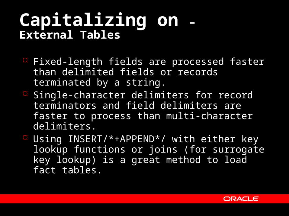
Fixed-length fields are processed faster than delimited fields or records terminated by a string.
Single-character delimiters for record terminators and field delimiters are faster to process than multi-character delimiters.
Using INSERT/*+APPEND*/ with either key lookup functions or joins (for surrogate key lookup) is a great method to load fact tables.

Capitalizing on – merge
Merge: Enables you to perform updates to matched
records and inserts of new records. Leverages parallelism Is a slick way of performing slowly changing
dimension logic.

Capitalizing on – merge
Cust ID Cust name City State Zip
7396 George W. Hayduke Athens GA 30605
7400 Seldom S. Smith Phoenix AZ 85003
7404 Edward Abby Phoenix AZ 85003
MERGE INTO CUSTOMERSUSING ( CUST_EXT x)WHEN MATCHED THENUPDATE SET city = x.city…WHEN NOT MATCHED THENINSERT (CUST_ID…)VALUES(x.cust_id…)
Customer Extract ExternalCust ID Cust Name City State Zip
7396 George W. Hayduke MOAB UT 84532
7400 Seldom S. Smith MOAB UT 84532
7404 Edward Abby MOAB UT 84532
7397 Doc Sarvis MOAB UT 84532
New
Cust ID Cust Name City State Zip
7396 George W. Hayduke MOAB UT 84532
7400 Seldom S. Smith MOAB UT 84532
7404 Edward Abby MOAB UT 84532
7397 Doc Sarvis MOAB UT 84532
Customer Existing Table
Customer Post Merge Matched updated

Capitalizing on – merge
Source Extract
Master Dimension Cross Reference
CompareNew & Changed
Records
Update Existing
Generate Key
Insert New
Typical type 1 slowly changing dimension (SCD) logic

Capitalizing on – merge for type 1 SCD
Capitalize on MERGE for Type 1 SCDs Steps:1. Create your dimension table2. Create an external table as your “extract
table” that contains all of the columns in your dimension except the surrogate key
3. Create an Oracle sequence this will be used for the surrogate key of your dimension
4. Use MERGE to populate your dimension

Capitalizing on – merge for type 1 SCD
1. Create our Dimension (Target) table
CREATE TABLE CUSTOMER_DIM ( CUST_KEY NUMBER NOT NULL, CUST_ID NUMBER NOT NULL, CUST_NAME VARCHAR2(20) NOT NULL, ZIP CHAR(5) NOT NULL, CITY VARCHAR2(30) NOT NULL, STATE VARCHAR2(40) NULL,CONSTRAINT CUSTOMER_PK PRIMARY KEY (CUST_KEY));
Note:
cust_key is our the surrogate key;
cust_id is the “natural key” or production key;

Capitalizing on – merge for type 1 SCD
2. Create our extract or “staging” table
CREATE TABLE CUSTOMER_EXTRACT( CUST_KEY NUMBER, CUST_ID NUMBER, CUST_NAME VARCHAR2(20), ZIP CHAR(5) , CITY VARCHAR2(30) , STATE VARCHAR2(40))ORGANIZATION EXTERNAL ( TYPE oracle_loader DEFAULT DIRECTORY extracts_dirACCESS PARAMETERS ( RECORDS DELIMITED BY NEWLINE CHARACTERSET US7ASCIIBADFILE log_file_dir:'customer_extract.bad' LOGFILE log_file_dir:'customer_extract.log' FIELDS TERMINATED BY "|" LDRTRIM ) location ( 'cust_extract.dat' ))REJECT LIMIT UNLIMITED PARALLEL;
2a. Running a new extract is simply a matter of referencing a new file:
ALTER TABLE customer_extractLOCATION (‘CIF_NOV_2003.dat‘);

Capitalizing on – merge for type 1 SCD
3. Create our Sequence – this will used for the surrogate key
CREATE SEQUENCE CUST_SEQ START WITH 1000 INCREMENT BY 1000;

Capitalizing on – merge for type 1 SCD
4. Use a single MERGE statement to perform our type 1 SCD logic
MERGE INTO CUSTOMER_DIM cUSING CUSTOMER_EXTRACT XON (c.cust_id = x.cust_id)WHEN MATCHED THENUPDATE SET CUST_FIRST_NAME = X.CUST_FIRST_NAME,CUST_LAST_NAME = X.CUST_LAST_NAME,….CUST_EMAIL = X.CUST_EMAILWHEN NOT MATCHED THENINSERT (CUST_KEY,CUST_ID,…)VALUES(CUST_SEQ.NEXTVAL,X.CUST_ID,…X.CUST_EMAIL);
Cust Key Cust ID Cust Name City State Zip
1000 7396 George W. Hayduke MOAB UT 84532
2000 7400 Seldom S. Smith MOAB UT 84532
3000 7404 Edward Abby MOAB UT 84532
4000 7397 Doc Sarvis MOAB UT 84532
Capitalizing on – merge
Cust Key Cust ID Cust name City State Zip
1000 7396 George W. Hayduke Athens GA 30605
2000 7400 Seldom S. Smith Phoenix AZ 85003
3000 7404 Edward Abby Phoenix AZ 85003
Customer Extract ExternalCust ID Cust Name City State Zip
7396 George W. Hayduke MOAB UT 84532
7400 Seldom S. Smith MOAB UT 84532
7404 Edward Abby MOAB UT 84532
7397 Doc Sarvis MOAB UT 84532
New
Existing Customer Dimension
Customer Dimension Post Merge
Matched updated
New
Updates

Capitalizing on – merge for type 2 SCD
Cust Key Cust ID Cust Name City State Zip Create Date
1000 7396 George W. Hayduke ATHENS GA 30605 Mar 15, 2000
5000 7396 George W. Hayduke MOAB UT 84532 Jan 16, 2003
2000 7400 Seldom S. Smith MOAB UT 84532 Jan 15, 2003
3000 7404 Edward Abby MOAB UT 84532 Jan 15, 2003
4000 7397 Doc Sarvis MOAB UT 84532 Jan 15, 2003
Change PointerSurrogate Key
Type 2 Slowly Changing Dimension (SCD) : Type 2 SCD a technique where a new dimension record is
created with a new surrogate key each to reflect the change We can do this quite simply a single merge statement simply add
the change columns to the ON () portion of the merge.MERGE INTO CUSTOMER_DIM cUSING CUSTOMER_EXTRACT XON (c.cust_id = x.cust_id and c.city=x.city and c.state=x.state and c.zip = x.zip)WHEN MATCHED THENUPDATE SET CUST_NAME = X.CUST_NAME,City = X.CITY, STATE=X.STATE, Zip=X.ZIP….WHEN NOT MATCHED THENINSERT (CUST_KEY,CUST_ID,CUST_NAME, CITY, STATE, ZIP, CREATE_DATE)VALUES(CUST_SEQ.NEXTVAL, /* CUST_KEY */X.CUST_ID,X.CUST_NAME…TRUNC(SYSDATE)); /* CREATE_DATE */
Change Columns

Capitalizing on – merge for type 2 SCD
Cust Key Cust ID Cust Name City State Zip Start Date End Date Current Flag
1000 7396 George W. Hayduke ATHENS GA 30605 Mar 15, 2000 Jan 15, 2003 N
5000 7396 George W. Hayduke MOAB UT 84532 Jan 16, 2003 Jan 1, 2099 Y
2000 7400 Seldom S. Smith MOAB UT 84532 Jan 15, 2003 Jan 1, 2099 Y
3000 7404 Edward Abby MOAB UT 84532 Jan 15, 2003 Jan 1, 2099 Y
4000 7397 Doc Sarvis MOAB UT 84532 Jan 15, 2003 Jan 1, 2099 Y
Change PointersSurrogate
Key
A more common approach to Type 2 Slowly Changing Dimension logic is the addition of change pointers for reference data, Unfortunately, this requires a multi-step process.
This is generally performed with a series of insert and update statements or procedural logic but can be accomplished with two merge statements as well.
– One to insert new records and update existing (close out)– One to insert new changed records

Capitalizing on – merge for type 2 SCD
/* First Merge: Close out existing, Insert New */ MERGE INTO CUST_DIM CUSING (SELECT cust_id, cust_name, city, state, zip FROM CUST_EXTRACT MINUS SELECT cust_id, cust_name, city, state, zip FROM CUST_DIM WHERE CURRENT_FLAG = 'Y') XON (C.CUST_ID = X.CUST_ID AND C.END_DATE=to_date('15-JAN-2099','DD-MON-YYYY'))WHEN MATCHED THEN UPDATE SET c.current_flag = 'N'WHEN NOT MATCHED THENINSERT (CUST_KEY,CUST_ID,CUST_NAME,CITY,STATE,ZIP,START_DATE,END_DATE,CURRENT_FLAG)VALUES( CUST_SEQ.NEXTVAL,X.CUST_ID,X.CUST_NAME,X.CITY,X.STATE,X.ZIP,trunc(SYSDATE),TO_DATE(‘01-JAN-2099','DD-MON-YYYY'),'Y');COMMIT;
/* Second Merge: Insert new changed record */MERGE INTO CUST_DIM CUSING ( SELECT cust_id, cust_name, city, state, zip FROM CUST_EXTRACT MINUSSELECT cust_id, cust_name, city, state, zip FROM CUST_DIM) XON (C.CUST_ID = X.CUST_ID AND C.CURRENT_FLAG='Y')WHEN MATCHED THENUPDATE SET c.END_DATE=trunc(SYSDATE -1)WHEN NOT MATCHED THENINSERT (CUST_KEY,CUST_ID,CUST_NAME,CITY,STATE,ZIP,START_DATE,END_DATE,CURRENT_FLAG)VALUES( CUST_SEQ.NEXTVAL,X.CUST_ID,X.CUST_NAME,X.CITY,X.STATE,X.ZIP,trunc(SYSDATE),TO_DATE(‘01-JAN-2099','DD-MON-YYYY'),'Y');COMMIT;
/*+ Final step Date Closeout */UPDATE CUST_DIM CSET c.END_DATE=trunc(SYSDATE -1)WHERE C.CURRENT_FLAG = 'N' AND c.END_DATE=TO_DATE(‘01-JAN-2099','DD-MON-YYYY');commit;
1 2
3

Capitalizing on – merge for type 2 SCD
Cust Key Cust ID Cust Name City State Zip Start Date End Date Current Flag
1000 7396 George W. Hayduke ATHENS GA 30605 Mar 15, 2000 Jan 1, 2099 Y
2000 7400 Seldom S. Smith MOAB UT 84532 Jan 15, 2003 Jan 1, 2099 Y
3000 7404 Edward Abby MOAB UT 84532 Jan 15, 2003 Jan 1, 2099 Y
Customer Extract ExternalCust ID Cust Name City State Zip
7396 George W. Hayduke MOAB UT 84532
7400 Seldom S. Smith MOAB UT 84532
7404 Edward Abby MOAB UT 84532
7397 Doc Sarvis MOAB UT 84532
Customer Existing Dimension
Customer Post Type 2 Merge (s)Cust Key Cust ID Cust Name City State Zip Start Date End Date Current Flag
1000 7396 George W. Hayduke ATHENS GA 30605 Mar 15, 2000 Jan 15, 2003 N
5000 7396 George W. Hayduke MOAB UT 84532 Jan 16, 2003 Jan 1, 2099 Y
2000 7400 Seldom S. Smith MOAB UT 84532 Jan 15, 2003 Jan 1, 2099 Y
3000 7404 Edward Abby MOAB UT 84532 Jan 15, 2003 Jan 1, 2099 Y
4000 7397 Doc Sarvis MOAB UT 84532 Jan 15, 2003 Jan 1, 2099 Y
Take note of how a single table design decision has impacted our ability to parallelize. Instead of a single merge statement we now have a three step process.

Capitalizing on – multiple inserts
Multiple Inserts: Enables us to conditionally insert into multiple
tables in parallel.– All: result set is applied to all conditions– First: result set is applied to the first condition
Leverages parallelism Is a slick way to segment data and load fact
tables.

Capitalizing on – multiple inserts
Multiple Inserts (ALL)
INSERT ALL WHEN state='GA‘ or state = ‘FL’ THEN INTO GA_SALES VALUES(prod_id, cust_id,sale_date,sale_amount qty_sold)WHEN state = 'FL' THEN INTO FL_SALES VALUES(prod_id, cust_id,sale_date,sale_amount qty_sold)ELSE INTO ALL_OTHER_SALES VALUES(prod_id, cust_id,sale_date,sale_amount qty_sold)SELECT prod_id, cust_id,sale_date,sale_amount qty_sold FROM sales_extract;
Prod ID Cust ID Sale Date Sale Amount
Qty Sold
State
1001 7396 Aug 14, 2003 $10 2 GA
1001 7400 Aug 14, 2003 $20 4 GA
1003 7404 Aug 14, 2003 $5 1 GA
1001 7396 Aug 14, 2003 $10 2 FL
1001 7400 Aug 14, 2003 $20 4 FL
1003 7404 Aug 14, 2003 $5 1 FL
Prod ID
Cust ID Sale Date Sale Amount
Qty Sold State
1001 7396 Aug 14, 2003 $10 2 FL
1001 7400 Aug 14, 2003 $20 4 FL
1003 7404 Aug 14, 2003 $5 1 FL
Prod ID
Cust ID Sale Date Sale Amount
Qty Sold State
1001 7396 Aug 14, 2003 $10 2 SC
1001 7400 Aug 14, 2003 $20 4 TX
1003 7404 Aug 14, 2003 $5 1 KY
GA_SALES
FL_SALES
ALL_OTHER_SALES
Que
ry

Capitalizing on – multiple inserts
Multiple Inserts (FIRST)INSERT FIRST
WHEN state ='GA‘ OR state = ‘FL’ THEN INTO GA_SALES VALUES(prod_id, cust_id,sale_date,sale_amount qty_sold)WHEN state = 'FL' THEN INTO FL_SALES VALUES(prod_id, cust_id,sale_date,sale_amount qty_sold)ELSE INTO ALL_OTHER_SALES VALUES(prod_id, cust_id,sale_date,sale_amount qty_sold)SELECT prod_id, cust_id,sale_date,sale_amount qty_sold FROM sales_extract;
Prod ID
Cust ID
Sale Date Sale Amount
Qty Sold State
1001 7396 Aug 14, 2003 $10 2 GA
1001 7400 Aug 14, 2003 $20 4 GA
1003 7404 Aug 14, 2003 $5 1 GA
1001 7396 Aug 14, 2003 $10 2 FL
1001 7400 Aug 14, 2003 $20 4 FL
1003 7404 Aug 14, 2003 $5 1 FL
Prod ID
Cust ID Sale Date Sale Amount
Qty Sold State
Prod ID
Cust ID Sale Date Sale Amount
Qty Sold State
1001 7396 Aug 14, 2003 $10 2 SC
1001 7400 Aug 14, 2003 $20 4 TX
1003 7404 Aug 14, 2003 $5 1 KY
GA_SALES
FL_SALES
ALL_OTHER_SALES

Capitalizing on - Partitioning
Types of Partitioning Range - maps rows to partitions based on ranges of column values
List (New) - enables you to explicitly control how rows map to partitions.
Hash - evenly distributes rows among partitions
Composite – Range-Hash: benefits of range partitioning then further hash
distributing the sub-partition. Partition pruning & Parallel processing
– Range List (New for 9i): benefits of range partitioning and
further discrete sub-partitioning.

Capitalizing on - Partitioning
Why is partitioning important“partitioning enables you to split large volumes of
data into smaller separate buckets that can be managed independently”
– Partition Pruning / Elimination– Partition-wise Joins– Parallel DML– Partition Exchanging / Swapping

Capitalizing on Oracle 9i partitioning
Why Partition?– Partition pruning
“Ability to eliminate partitions that don’t satisfy query conditions”
Jan 2003
Feb 2003
Mar 2003
…
SELECT sum(qty_sold)
FROM sales
WHERE sale_date
BETWEEN Feb 1, 2003
and Feb 15, 2003

Capitalizing on Oracle 9i partitioning
Why Partition? Partition-wise joins Full – Equi-partitioned on
the join keys i.e. the two tables are both partitioned on the same key. Hash-Hash is the easiest example.
Partial – Oracle dynamically repartitions based on the reference table.
Here accounts and transactions are both hash partitioned by account_id into 32 partitions Note: to achieve equal work distribution, the
number of partitions should always be a multiple of the degree of parallelism. Ex. Here we hashed account and transaction into 32 partitions with a degree of parallelism 8
P1
P1
P2
P2
P3
P3
Pnn
Pnn
Accounts
Transactions
Server Server Server ServerParallel
ExecutionServers

Capitalizing on Oracle 9i partitioning
7396 John Smith
7400 Leslie Baker
7404 Sarah Duncan
7398 Jean Doyle
7402 Dan Peters
7406 Terry Jones
7397 Kevin Allen
7401 Cynthia Ward
7405 Greg Lange
7399 Lynn Dennis
7403 Karen Shaw
7407 Chris Albert
7396 $1.23 5
7400 $5.67 6
7404 $3.45 12
7398 $1.34 20
7402 $1.77 3
7406 $1.88 4
7397 $4.98 3
7401 $3.21 2
7405 $4.67 7
7399 $1.99 8
7403 $1.23 9
7407 $1.77 10
ACCT ID NAME ACCT ID Price QTY
Par
titio
n-w
ise
Join
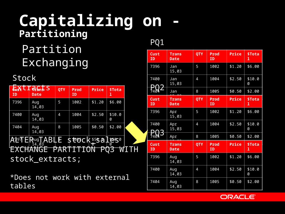
Capitalizing on - Partitioning
Cust ID Trans Date QTY Prod ID Price $Total
7396 Aug 14,03 5 1002 $1.20 $6.00
7400 Aug 14,03 4 1004 $2.50 $10.00
7404 Aug 14,03 8 1005 $0.50 $2.00
7397 Aug 14,03 1 1003 $50.00 $50.00
Cust ID Trans Date QTY Prod ID Price $Total
7396 Jan 15,03 5 1002 $1.20 $6.00
7400 Jan 15,03 4 1004 $2.50 $10.00
7404 Jan 15,03 8 1005 $0.50 $2.00
Cust ID Trans Date QTY Prod ID Price $Total
7396 Apr 15,03 5 1002 $1.20 $6.00
7400 Apr 15,03 4 1004 $2.50 $10.00
7404 Apr 15,03 8 1005 $0.50 $2.00
Cust ID Trans Date QTY Prod ID Price $Total
7396 Aug 14,03 5 1002 $1.20 $6.00
7400 Aug 14,03 4 1004 $2.50 $10.00
7404 Aug 14,03 8 1005 $0.50 $2.00
PQ1
PQ2
PQ3ALTER TABLE stock_salesEXCHANGE PARTITION PQ3 WITH stock_extracts;
*Does not work with external tables
Stock Extracts
Partition Exchanging

Capitalizing on - Partitioning
CREATE TABLE account_balance_range(account_key NUMBER(7) CONSTRAINT acct_nn NOT NULL, branch_key NUMBER(7) CONSTRAINT brch_nn NOT NULL,product_key NUMBER(7) CONSTRAINT prod_nn NOT NULL,snapshot_date DATE CONSTRAINT mnth_nn NOT NULL,state_key CHAR(2) CONSTRAINT stat_nn NOT NULL,ending_bal NUMBER(7,3) CONSTRAINT ebal_nn NOT NULL,average_daily_bal NUMBER(7,3) CONSTRAINT abal_nn NOT NULL,transaction_count NUMBER(7) CONSTRAINT txnc_nn NOT NULL,interest_paid NUMBER(7,3) CONSTRAINT intp_nn NOT NULL,fees_charged NUMBER(7,3) CONSTRAINT feec_nn NOT NULL)PARTITION BY RANGE (snapshot_date)(PARTITION Q1_ACCT_BAL VALUES LESS THAN (TO_DATE('01-APR-2000','DD-MON-YYYY')),PARTITION Q2_ACCT_BAL VALUES LESS THAN (TO_DATE('01-JUL-2000','DD-MON-YYYY')),PARTITION Q3_ACCT_BAL VALUES LESS THAN (TO_DATE('01-OCT-2000','DD-MON-YYYY')),PARTITION Q4_ACCT_BAL VALUES LESS THAN (TO_DATE('01-JAN-2001','DD-MON-YYYY')));
Range Example

Slick New Feature - Partitioning
CREATE TABLE account_balance_list(account_key NUMBER(7) CONSTRAINT acct_nn NOT NULL, branch_key NUMBER(7) CONSTRAINT brch_nn NOT NULL,product_key NUMBER(7) CONSTRAINT prod_nn NOT NULL,snapshot_date DATE CONSTRAINT mnth_nn NOT NULL,state_key CHAR(2) CONSTRAINT stat_nn NOT NULL,ending_bal NUMBER(7,3) CONSTRAINT ebal_nn NOT NULL,average_daily_bal NUMBER(7,3) CONSTRAINT abal_nn NOT NULL,transaction_count NUMBER(7) CONSTRAINT txnc_nn NOT NULL,interest_paid NUMBER(7,3) CONSTRAINT intp_nn NOT NULL,fees_charged NUMBER(7,3) CONSTRAINT feec_nn NOT NULL)PARTITION BY LIST (state_key)(PARTITION northwest VALUES ('OR', 'WA'), PARTITION southwest VALUES ('AZ', 'UT', 'NM'),PARTITION southeast VALUES ('FL','GA','SC','AL','TN','NC'),PARTITION rest VALUES (DEFAULT))’);
List Example

Capitalizing on - Partitioning
CREATE TABLE account_balance_hash(account_key NUMBER(7) CONSTRAINT acct_nn NOT NULL, branch_key NUMBER(7) CONSTRAINT brch_nn NOT NULL,product_key NUMBER(7) CONSTRAINT prod_nn NOT NULL,snapshot_date DATE CONSTRAINT mnth_nn NOT NULL,state_key CHAR(2) CONSTRAINT stat_nn NOT NULLending_bal NUMBER(7,3) CONSTRAINT ebal_nn NOT NULL,average_daily_bal NUMBER(7,3) CONSTRAINT abal_nn NOT NULL,transaction_count NUMBER(7) CONSTRAINT txnc_nn NOT NULL,interest_paid NUMBER(7,3) CONSTRAINT intp_nn NOT NULL,fees_charged NUMBER(7,3) CONSTRAINT feec_nn NOT NULL)PARTITION BY HASH (account_key)(PARTITIONS 16STORE IN (TS1_DATA, TS2_DATA, TS3_DATA, TS4_DATA);
Hash Example

Capitalizing on - Partitioning
CREATE TABLE account_bal_range_hash(account_key NUMBER(7) CONSTRAINT acct_nn NOT NULL, branch_key NUMBER(7) CONSTRAINT brch_nn NOT NULL,product_key NUMBER(7) CONSTRAINT prod_nn NOT NULL,snapshot_date DATE CONSTRAINT mnth_nn NOT NULL,state_key CHAR(2) CONSTRAINT stat_nn NOT NULL,ending_bal NUMBER(7,3) CONSTRAINT ebal_nn NOT NULL,average_daily_bal NUMBER(7,3) CONSTRAINT abal_nn NOT NULL,transaction_count NUMBER(7) CONSTRAINT txnc_nn NOT NULL,interest_paid NUMBER(7,3) CONSTRAINT intp_nn NOT NULL,fees_charged NUMBER(7,3) CONSTRAINT feec_nn NOT NULL)PARTITION BY RANGE (snapshot_date)SUBPARTITION BY HASH (account_key) SUBPARTITIONS 8( PARTITION Q1_ACCT_BAL
VALUES LESS THAN (TO_DATE('01-APR-2000','DD-MON-YYYY')),PARTITION Q2_ACCT_BAL
VALUES LESS THAN (TO_DATE('01-JUL-2000','DD-MON-YYYY')),PARTITION Q3_ACCT_BAL
VALUES LESS THAN (TO_DATE('01-OCT-2000','DD-MON-YYYY')),PARTITION Q4_ACCT_BAL
VALUES LESS THAN (TO_DATE('01-JAN-2001','DD-MON-YYYY')));
Composite Range-Hash Example

Capitalizing on - Partitioning
CREATE TABLE account_bal_range_list(account_key NUMBER(7) CONSTRAINT acct_nn NOT NULL, branch_key NUMBER(7) CONSTRAINT brch_nn NOT NULL,product_key NUMBER(7) CONSTRAINT prod_nn NOT NULL,snapshot_date DATE CONSTRAINT mnth_nn NOT NULL,state_key CHAR(2) CONSTRAINT stat_nn NOT NULL,ending_bal NUMBER(7,3) CONSTRAINT ebal_nn NOT NULL,average_daily_bal NUMBER(7,3) CONSTRAINT abal_nn NOT NULL,transaction_count NUMBER(7) CONSTRAINT txnc_nn NOT NULL,interest_paid NUMBER(7,3) CONSTRAINT intp_nn NOT NULL,fees_charged NUMBER(7,3) CONSTRAINT feec_nn NOT NULL)PARTITION BY RANGE (snapshot_date)SUBPARTITION BY LIST (state)SUBPARTITION TEMPLATE(PARTITION northwest VALUES ('OR', 'WA'), PARTITION southwest VALUES VALUES ('AZ', 'UT', 'NM'),PARTITION southeast VALUES ('FL', 'GA','SC','AL','TN','NC'),PARTITION rest VALUES (DEFAULT)))(PARTITION q1_2002 VALUES LESS THAN(TO_DATE('1-APR-2002','DD-MON-YYYY')),PARTITION q2_2002 VALUES LESS THAN(TO_DATE('1-JUL-2002','DD-MON-YYYY')),PARTITION q3_2002 VALUES LESS THAN(TO_DATE('1-OCT-2002','DD-MON-YYYY')),PARTITION q4_2002 VALUES LESS THAN(TO_DATE('1-JAN-2003','DD-MON-YYYY')));
Composite Range-List Example

Capitalizing on - PartitioningS
ourc
e
Target
1. FTP 02Nov2003_Sales Extract2. “Alter Table” add file(s) to location3. Perform INSERT /*+Append*/ INTO partitioned table
External Table to Partition using INSERT /*+APPEND*/
File(s)

Capitalizing on – Partitioning
Cust ID Trans Date QTY Prod ID Price $Total
7396 Jan 15,03 5 1002 $1.20 $6.00
7400 Jan 15,03 4 1004 $2.50 $10.00
7404 Jan 15,03 8 1005 $0.50 $2.00
Cust ID Trans Date QTY Prod ID Price $Total
7396 Apr 15,03 5 1002 $1.20 $6.00
7400 Apr 15,03 4 1004 $2.50 $10.00
7404 Apr 15,03 8 1005 $0.50 $2.00
Cust ID Trans Date QTY Prod ID Price $Total
7396 Aug 14,03 5 1002 $1.20 $6.00
7400 Aug 14,03 4 1004 $2.50 $10.00
7404 Aug 14,03 8 1005 $0.50 $2.00
PQ1
PQ2
PQ3INSERT/*+APPEND*/ INTO SALES (PQ3)SELECT * FROM SALES_EXTRACT_EXTERNAL
Sales Extract External
Cust ID Trans Date QTY Prod ID Price $Total
7396 Aug 15,03 5 1002 $1.20 $6.00
7400 Aug 15,03 4 1004 $2.50 $10.00
7404 Aug 15,03 8 1005 $0.50 $2.00
7397 Aug 15,03 1 1003 $50.00 $50.00

Capitalizing on – Partitioning
What to partition:– Fact Tables
Generally Range-Hash composite Range for some date (partition elimination) Hash on the driving dimension key (partition-wise join)
– Dimension Hashing on the primary key of dimension tables facilitates full
and partial partition-wise joins. To for a full partition-wise join between a fact and dimension
table you need to hash partition on the same key in the same number of buckets.
– Materialized Views Generally Range-Hash composite Generally mirror the fact tables partition scheme

Capitalizing on – Materialized Views
Materialized Views Enable queries to be re-written to take advantage of pre-calculated
summaries thus reducing or eliminating sorts and joins.
Materialized Views can dramatically increase performance of queries when applied judiciously:
– Reduce the number of sorts– Reduce the number of joins – Pre-filters data– Can be Indexed and Partitioned– Seamless to end users
Enhancements in 9i include– Removed restrictions enabling them to be leveraged in more situations– Fast refresh is now possible on a materialized views containing the
UNION ALL operator.

Capitalizing on – Materialized Views
Materialized Views cont…
SELECT T.FISCAL_QUARTER_DESC, C.CUST_CITY, COUNT(*) AS SALE_COUNT, SUM(S.AMOUNT_SOLD) AS SALE_DOLLARSFROM oradata.CUSTOMERS C, oradata.SALES S, oradata.TIMES TWHERE C.CUST_ID = S.CUST_ID AND T.TIME_ID = S.TIME_IDGROUP BY T.FISCAL_QUARTER_DESC, C.CUST_CITY Query is re-written to be
resolved from the MV instead of from the base tables

Capitalizing on – Materialized Views
How to capitalize on MVs– Identify candidate queries
Analysis of common queries based on design Oracle’s Summary Advisor & Wizard DBMS_OLAP
– Create MVs based on analysis and refresh requirements. Test Benchmark Measure Utilization Repeat

Capitalizing on – Materialized Views
proc sql;/* CTAS Implicit Pass-Through */CREATE TABLE work.quartly_city_canidateAS SELECT T.FISCAL_QUARTER_DESC, C.CUST_CITY, COUNT(*) AS SALE_COUNT, SUM(S.AMOUNT_SOLD) AS SALE_DOLLARSFROM oradata.CUSTOMERS C, oradata.SALES S, oradata.TIMES TWHERE C.CUST_ID = S.CUST_ID AND T.TIME_ID = S.TIME_IDGROUP BY T.FISCAL_QUARTER_DESC, C.CUST_CITY;quit;
real time 9.62 seconds
Execution Plan---------------------------------------------------------- 0 SELECT STATEMENT Optimizer=CHOOSE (Cost=5392 Card=7453 Bytes350291) 1 0 SORT (GROUP BY) (Cost=5392 Card=7453 Bytes=350291) 2 1 HASH JOIN (Cost=1077 Card=1016271 Bytes=47764737) 3 2 TABLE ACCESS (FULL) OF 'TIMES' (Cost=6 Card=1461 Bytes23376) 4 2 HASH JOIN (Cost=1043 Card=1016271 Bytes=31504401) 5 4 TABLE ACCESS (FULL) OF 'CUSTOMERS' (Cost=106 Card=50000 Bytes=700000) 6 4 PARTITION RANGE (ALL) 7 6 TABLE ACCESS (FULL) OF 'SALES' (Cost=469 Card=1016271 Bytes=17276607)Statistics----------------------------------------------------------5855 consistent gets1 sorts (memory)0 sorts (disk)5075 rows processed
Note the Number of Joins and Sorts, the amount of memory, and the number of full table scans.

Capitalizing on – Materialized Views
Question did it improve the performance of our query?
proc sql;connect to ORACLE as ORACON (user=sh password=sh1 path=‘demo.na.sas.com');/* Create a Materialized View */execute (CREATE MATERIALIZED VIEW QTRLY_CITY_SALES_MVcompressBUILD IMMEDIATEREFRESH ON COMMITENABLE QUERY REWRITEASSELECT T.FISCAL_QUARTER_DESC, C.CUST_CITY, COUNT(*) SALE_COUNT, SUM(S.AMOUNT_SOLD) SALE_DOLLARSFROM CUSTOMERS C, SALES S, TIMES TWHERE C.CUST_ID = S.CUST_ID AND T.TIME_ID = S.TIME_IDGROUP BY T.FISCAL_QUARTER_DESC, C.CUST_CITY) by ORACON;disconnect from ORACON;quit;
Build Immediate = Create this Now
Refresh on Commit = Keep the MV current when Insert, Update, and Deletes occur
Enable Query Rewrite = Enables dynamic query re-direction.
Compress = compresses redundant data i.e. makes the MV smaller

Capitalizing on – Materialized Views
proc sql;/* CTAS Implicit Pass-Through */CREATE TABLE work.quartly_city_canidateAS SELECT T.FISCAL_QUARTER_DESC, C.CUST_CITY, COUNT(*) AS SALE_COUNT, SUM(S.AMOUNT_SOLD) AS SALE_DOLLARSFROM oradata.CUSTOMERS C, oradata.SALES S, oradata.TIMES TWHERE C.CUST_ID = S.CUST_ID AND T.TIME_ID = S.TIME_IDGROUP BY T.FISCAL_QUARTER_DESC, C.CUST_CITY;quit;
Real Time 0.76 seconds
Execution Plan---------------------------------------------------------- 0 SELECT STATEMENT Optimizer=CHOOSE (Cost=4 Card=2206 Bytes=114712) 1 0 TABLE ACCESS (FULL) OF 'QTRLY_CITY_SALES_MV' (Cost=4 Card=2206 Bytes=114712)Statistics---------------------------------------------------------- 7 recursive calls 0 db block gets 366 consistent gets 0 physical reads 0 redo size 137260 bytes sent via SQL*Net to client 2641 bytes received via SQL*Net from client 340 SQL*Net roundtrips to/from client 0 sorts (memory) 0 sorts (disk) 5075 rows processed
No Joins, No Sorts, Less Memory…

Capitalizing on – Alt aggregate strategies
Aggregate building with pCTAS
CREATE TABLE quartly_city_passthrough PARALLEL NOLOGGING asSELECT T.FISCAL_QUARTER_DESC, C.CUST_CITY, COUNT(*) AS SALE_COUNT, SUM(S.AMOUNT_SOLD) AS SALE_DOLLARS
FROM CUSTOMERS C, SALES S, TIMES T
WHERE C.CUST_ID = S.CUST_ID AND T.TIME_ID = S.TIME_ID
GROUP BY T.FISCAL_QUARTER_DESC, C.CUST_CITY

Capitalizing on – Alt aggregate strategies
Aggregate building with pIIAS
INSERT /*+ APPEND */ INTO quartly_city_iiasSELECT T.FISCAL_QUARTER_DESC, C.CUST_CITY, COUNT(*) AS SALE_COUNT, SUM(S.AMOUNT_SOLD) AS SALE_DOLLARSFROM CUSTOMERS C, SALES S, TIMES TWHERE C.CUST_ID = S.CUST_ID AND T.TIME_ID = S.TIME_IDGROUP BY T.FISCAL_QUARTER_DESC, C.CUST_CITY

Capitalizing on – bitmap join index
Bitmap Join Index Creates a bitmap index for the resolution of joins of
two or more tables. Works similar to a materialized view.
Bitmap join index is space efficient because it compresses the rowids where a materialized view does not.
Can be leveraged to improve performance of snowflake schemas and common join operations across facts.

CREATE BITMAP INDEX bjx_sales_country
ON sales(countries.country_name))
FROM sales, customers, countries
WHERE sales.cust_id = customers.cust_id
AND countries.country_id = customers.country_id
LOCAL PARALLEL NOLOGGING COMPUTE STATISTICS;
Capitalizing on – bitmap join index
SELECT countries.country_name, sum(sales.amount_sold)FROM sales, customers, countriesWHERE sales.cust_id = customers.cust_idAND customers.country_id = countries.country_id…
Can be leveraged to improve performance of snowflake query problems
SALES_FACT
cust_id (FK)prod_id (FK)time_id (FK)channel_id (FK)promo_id (FK)quantity_soldamount_sold
CUSTOMER_DIM
cust_id (PK)cust_namestreet_addresscitystatecountry_id (FK)phone_number
COUNTRY_DIM
country_id (PK)country_namecountry_region

Capitalizing on – SQL for Analysis
SQL for Analysis Especially useful for reporting and preparing data sets for
statistical analysis– Rankings and percentiles
cumulative distributions, percent rank, and N-tiles.– Moving window calculations
allow you to find moving and cumulative aggregations, such as sums and averages.
– Lag/lead analysis enables direct inter-row references so you can calculate
period-to-period changes.– First/last analysis
first or last value in an ordered group.

Capitalizing on – SQL for Analysis
RANK– RANK ( ) OVER ( [query_partition_clause] order_by_clause )– DENSE_RANK ( ) OVER ( [query_partition_clause] order_by_clause )
SELECT country_id,TO_CHAR(SUM(amount_sold), '9,999,999,999') Sales_Total,RANK() OVER (ORDER BY SUM(amount_sold) DESC NULLS LAST) AS sales_leaderFROM sales, products, customers, times, channelsWHERE sales.prod_id=products.prod_id AND
sales.cust_id=customers.cust_id ANDsales.time_id=times.time_id ANDsales.channel_id=channels.channel_id ANDtimes.calendar_month_desc IN ('2000-09', '2000-10')
GROUP BY country_id;
CO SALES_TOTAL SALES_LEADER-- -------------- ------------US 13,333,510 1NL 7,174,053 2UK 6,421,240 3DE 6,346,440 4FR 4,404,921 5ES 1,699,209 6IE 1,549,407 7IN 732,502 8AU 632,475 9BR 606,281 10

Capitalizing on – SQL for Analysis
Rank for Top N
SELECT * FROM(SELECT country_id,
TO_CHAR(SUM(amount_sold), '9,999,999,999') Sales_Total,
RANK() OVER (ORDER BY SUM(amount_sold) DESC NULLS LAST) AS sales_leaderFROM sales, products, customers, times, channelsWHERE sales.prod_id=products.prod_id ANDsales.cust_id=customers.cust_id ANDsales.time_id=times.time_id ANDsales.channel_id=channels.channel_id AND times.calendar_month_desc IN ('2000-09', '2000-10')GROUP BY country_id ) /* inline view */WHERE COUNTRY_RANK <= 10;
CO SEPT_TOTAL COUNTRY_RANK-- -------------- ------------US 6,517,786 1NL 3,447,121 2UK 3,207,243 3DE 3,194,765 4FR 2,125,572 5ES 777,453 6IE 770,758 7IN 371,198 8BR 317,001 9AU 302,393 10

SELECT c.country_id AS CO, t.calendar_quarter_desc AS QUARTER,TO_CHAR (SUM(amount_sold), '9,999,999,999') AS Q_SALES,TO_CHAR(SUM(SUM(amount_sold)) OVER (PARTITION BY c.country_id ORDER BY c.country_id, t.calendar_quarter_desc ROWS UNBOUNDED PRECEDING), '9,999,999,999') AS RUNNING_TOTALFROM sales s, times t, customers cWHERE s.time_id=t.time_id ANDs.cust_id=c.cust_id ANDt.calendar_year=2000GROUP BY c.country_id, t.calendar_quarter_descORDER BY c.country_id, t.calendar_quarter_desc;
Capitalizing on – SQL for Analysis
Moving window Example: running total
CO QUARTER Q_SALES RUNNING_TOTALUS 2000-Q1 21,719,528 21,719,528US 2000-Q2 21,915,534 43,635,062US 2000-Q3 18,857,276 62,492,338US 2000-Q4 14,970,316 77,462,654

Capitalizing on – SQL for Analysis
SELECT c.country_id AS CO, t.calendar_month_desc AS CAL,TO_CHAR (SUM(amount_sold), '9,999,999,999') AS SALES ,TO_CHAR(AVG(SUM(amount_sold)) OVER (ORDER BY c.country_id, t.calendar_month_desc ROWS 2 PRECEDING),'9,999,999,999') AS MOVING_3_MONTHFROM sales s, times t, customers cWHERE s.time_id=t.time_id AND s.cust_id=c.cust_id AND t.calendar_year=2000 GROUP BY c.country_id, t.calendar_month_descORDER BY c.country_id, t.calendar_month_desc;
Moving window Example: moving average
CO CALENDAR SALES MOVING_3_MONTH-- -------- -------------- --------------AR 2000-01 172,380 172,380AR 2000-02 140,906 156,643AR 2000-03 142,581 151,956AR 2000-04 169,727 151,071AR 2000-05 157,016 156,441AR 2000-06 155,675 160,806

Capitalizing on – SQL for Analysis
LAG / LEAD
SELECT time_id, TO_CHAR(SUM(amount_sold),'9,999,999') AS SALES,TO_CHAR(LAG(SUM(amount_sold),1) OVER (ORDER BY time_id),'9,999,999') AS LAG1,TO_CHAR(LAG(SUM(amount_sold),2) OVER (ORDER BY time_id),'9,999,999') AS LAG2,TO_CHAR(LEAD(SUM(amount_sold),1) OVER (ORDER BY time_id),'9,999,999') AS LEAD1,TO_CHAR(LEAD(SUM(amount_sold),2) OVER (ORDER BY time_id),'9,999,999') AS LEAD2FROM sales WHERE time_id between TO_DATE('01-JAN-2000') AND TO_DATE('31-JAN-2000')GROUP BY time_id;
TIME_ID SALES LAG1 LAG2 LEAD1 LEAD2--------- ---------- ---------- ---------- ---------- ----------01-JAN-00 869,132 909,726 896,62602-JAN-00 909,726 869,132 896,626 895,20403-JAN-00 896,626 909,726 869,132 895,204 954,06604-JAN-00 895,204 896,626 909,726 954,066 918,15405-JAN-00 954,066 895,204 896,626 918,154 895,84906-JAN-00 918,154 954,066 895,204 895,849 889,525

Capitalizing on – SQL for Analysis
FIRST/LAST lets you order on column A but return an result of an aggregate applied on column B.
SELECT prod_subcategory, MIN(prod_list_price) KEEP (DENSE_RANK FIRST ORDER BY (prod_min_price)) AS LPLO_MINP,MIN(prod_min_price) AS LO_MINP, MAX(prod_list_price) KEEP (DENSE_RANK LAST ORDER BY (prod_min_price))AS LPHI_MINP,MAX(prod_min_price) AS HI_MINPFROM productsWHERE prod_category='Women'GROUP BY prod_subcategory;PROD_SUBCATEGORY LPLO_MINP LO_MINP LPHI_MINP HI_MINP
------------------------- ------------- ---------- ------------- ----------
Dresses - Women 44 31.28 189 165
Easy Shapes - Women 51 39.47 149 127.39
Knit Outfits - Women 38 17.78 138 95.63
Outerwear - Women 58 27.14 198 131.87
Shirts And Jackets - Women 19 13.68 162 145.8
• List price of the product with the lowest minimum price LPLO_MINP• Lowest minimum price LO_MINP• List price of the product with the highest minimum price LPHI_MINP• Highest minimum price HI_MINP

Other Important New Features
Table Compression
Multiple Block Sizes
RAC for warehousing

Capitalizing on Table Compression Table Compression:
– Can improve performance by reducing both disk and memory (buffer cache) requirements.
Note: tables with large amounts of DML operations are not good candidates for compression
– Ideal candidates are partitioned fact tables, materialized views with rollups, and tables with a high degree of redundant data
– Regular tables create table (…) compress alter table compress
– Partitioned tables Can compress the entire table or on a partition by partition basis Create table (…) compress partition by (…) PARTITION p1 VALUES (‘FL', ‘GA') COMPRESS
– Materialized Views CREATE MATERIALIZED VIEW QTRLY_SALES_MV COMPRESS Alter materialized view … compress

Capitalizing on Multiple Block Sizes
Multiple Block Size Capitalization:– When you need to run a mix of OLTP activity and
DSS activity within the same instance– When you have an OLTP system with a smaller
block sizes and using transportable tablespaces to move tables to a decision support system.
– Place small static dimensions in a smaller block cache (4K or 8K) and larger dimensions and facts in a large block cache (16K)

Capitalizing on RAC
High Speed InterconnectHigh Speed Interconnect
Storage Area Network (SAN)
Node 1Node 1 Node 2Node 2 Node 3Node 3 Node NNode N

Capitalizing on RAC
RAC provides both speedup and scale up– Theoretically to double performance simply double the number of
nodes. – Limiting traffic over the interconnect is key to performance.
Parallel Loading Multiple SQL*Loader sessions Collocated extracts
Querying Partition key choices
Data model design choices Define join dependencies
– Partition wise joins are key to limiting the traffic over the interconnect. match partitions so that they are collocated on the same node
– Oracle’s automatic node affinity improves performance of DML operations by routing DML operations to the node that has affinity for the partition.

Conclusion
Parallelism is key to performance of DSS applications– Design is the limiting factor to parallelism and performance
Oracle has some slick new features that enhance and simplify common warehouse operations.
The future direction of data warehousing:– Better performance
Increased parallelism & reduced dependencies Loads Queries
– Reduced complexity & higher user satisfaction Better design paradigms and ideologies
– Enhanced features Increased usability Increased ability to capitalize

Next Steps….
Recommended sessions– Optimal Usage of Oracle's Partitioning Option– Oracle9i: The Features They Didn't Tell You About– Advanced PL/SQL and Oracle9i ETL– Oracle 9i RAC Concepts and Implementation - A Practical
Perspective

AQ&Q U E S T I O N SQ U E S T I O N S
A N S W E R SA N S W E R S
