How credible is the Federal Reserve? A structural

estimation of policy re-optimizations ∗

Davide Debortoli

UC San Diego, UPF and Barcelona GSE

Aeimit Lakdawala

Michigan State University

March 2014

Abstract

Using a Markov-switching Bayesian likelihood approach, the paper proposes a new

measure of the degree of credibility of the Federal Reserve. We estimate a medium-

scale macroeconomic model, where the central bank has access to a commitment tech-

nology, but where a regime-switching process governs occasional re-optimizations of

announced plans. The framework nests the commonly used discretion and commit-

ment cases, while allowing for a continuum of intermediate cases. Our estimates reject

both full-commitment and discretion. We instead identify occasional re-optimization

episodes that are consistent with changes in Federal Reserve policymakers and operat-

ing procedures. Finally, through counterfactual analysis we assess the role of credibility

over the past four decades.

JEL classification: C32, E58, E61.

Keywords: Commitment, Regime-Switching Bayesian Estimation, DSGE models

∗We thank Andrea Tambalotti for his discussion, and Jordi Galı, Jim Hamilton, Cosmin Ilut, TatianaKirsanova, Kristoffer Nimark, Ricardo Nunes, Valerie Ramey, Frank Schorfheide and seminar participantsat UCSD, Michigan State, SED annual meeting (Seoul), Federal Reserve Board, the mid-year meetingof the NBER “Methods and Applications for DSGE Models” group, Barcelona GSE Winter Forum andLancaster for their useful comments. All remaining errors are our own. Contact emails: ddebortoli@ucsd.edu,aeimit@msu.edu.

1

“Whether we have the credibility to persuade markets that we’ll follow through

is an empirical question.”

Ben Bernanke, Federal Reserve Chairman, September 13th 2012.

1 Introduction

Both academics and policymakers agree on the importance of central bank credibility in

conducting monetary policy. Over the past few decades significant effort has been devoted to

enhance credibility in monetary policy, through the creation of independent central banks,

the adoption of clear policy objectives, improved transparency and communication strategies,

among other measures. Whether central banks are indeed credible, however, remains a

largely open question. This paper proposes a novel measure of central bank credibility, and

provides new evidence about the credibility of the Federal Reserve over the past few decades.

The term credibility is used in practice to refer to a multiplicity of different concepts, As

surveyed by Blinder (2000), academics and policymakers identify the term “credibility” with

various different measures, such as “transparency”, “independence”, “aversion to inflation”,

etc. Our definition of credibility coincides with the notion of “commitment”, as in the

seminal works of Kydland and Prescott (1977) and Barro and Gordon (1983). The presence

of a policy trade-off (e.g. stabilizing inflation vs. output), combined with the forward looking

nature of economic agents, makes it desirable for the central bank to commit to a policy

plan. By committing to a plan, the central bank can shape agents’ expectations in a way

that improves the short-run policy tradeoffs. However, once those short-run benefits have

been reaped, there is an ex-post temptation to deviate from the original plan, and to re-

optimize. Credibility is then defined as the ability to resist the temptation to re-optimize.

This definition is widely accepted in the monetary policy literature, and is also consistent

with the central bank having a “a history of doing what it says it will do”, which both

academics and policymakers selected as the most important factor in building central bank

credibility in the survey by Blinder (2000).

The monetary policy literature has typically considered two alternative (and extreme)

scenarios about the central bank ability to commit. It has either assumed that the central

bank always follows its announced plans (commitment case), or that it always deviates

(discretion case). This paper adopts a more flexible approach based on the works by Roberds

(1987), Schaumburg and Tambalotti (2007) and Debortoli and Nunes (2010) that nests

2

commitment and discretion as special cases, while allowing for a continuum of intermediate

cases – i.e. the so-called loose commitment setting.1 The central bank has the ability to

commit to its future plans, but it may occasionally give in to the temptation to revise its

plans. Both the central bank and the private sector are aware of the possibility of policy

re-optimizations, and take it into account when forming expectations.

In particular, we consider a model where the behavior of the central bank is allowed

to change over time, according to a two-state regime-switching process. In each period,

with probability γ the central bank follows its previous plan, while with probability 1 − γit makes a new plan. The probability γ ∈ [0, 1] can then be interpreted as a measure

of credibility. In the limiting case where γ = 1 there would be no re-optimization (the

case of commitment), while if γ = 0 there would be a re-optimization in every period (the

case of discretion). Intermediate values of γ describe levels of credibility in between the

two extremes.2 This setting is meant to capture the fact that central bankers understand

the benefits of credibility, but at the same time there could be situations when a central

banks disregards its commitments. Possible candidates for such events are changes in the

dominating views within a central bank due to time-varying composition of its decision-

making committee or varying intensity of outside pressures by politicians and the financial

industry.3 This paper aims at identifying and characterizing policy re-optimizations, but

abstracts from analyzing their specific sources.

The empirical analysis is conducted within the medium-scale model for the US economy

of Smets and Wouters (2007) (henceforth SW). That model can be viewed as the backbone

of the estimated models developed at central banks in recent years, and used for monetary

policy analysis and forecasting. We depart from that model in two important ways. First,

monetary policies are chosen optimally by a central bank operating under loose commitment,

rather than being described by a simple (Taylor-type) rule. Second, we deal with a version of

1Roberds (1987) used the term “stochastic replanning” while Schaumburg and Tambalotti (2007) usedthe term “quasi-commitment”.

2Equivalently, that probability can be thought of as a continuous variable measuring the durability of theFederal Reserve’s promises, where longer durability corresponds to higher levels of credibility.

3In the case of the United States, the reserve bank presidents serve one-year terms as voting members of theFOMC on a rotating basis, except for the president of the New York Fed. Furthermore, substantial turnoveramong the reserve bank presidents and the members of the Board of Governors arises due to retirement andoutside options. With the (up to) seven members of the Board of Governors being nominated by the U.S.President and confirmed by the U.S. Senate, the composition of views in the FOMC may be affected bythe views of the political party in power at the time of the appointment. Chappell et al. (1993) and Bergerand Woitek (2005) find evidence of such effects in the U.S. and Germany, respectively. Also, the book byHavrilesky (1995) provides evidence on when politicians tried to influence monetary policy, and when theFederal Reserve did and did not respond.

3

the SW model with regime-switching. On top of the regime-switching process driving policy

re-optimizations described earlier, we also allow the variance of the shock processes to shift

over time to control for additional potential sources of time variation. Estimation is carried

out using a Bayesian Markov Chain Monte Carlo (MCMC) algorithm.

Two main results emerge from the estimates. First, the model supports the idea that the

Federal Reserve is to some extent credible, but that credibility is not perfect. This result

differs from the existing literature, as it signals that both the commonly used assumptions of

commitment and discretion are rejected by the data. Within a variety of different exercises,

the posterior mode of the unconditional probability of commitment is estimated to be about

0.80, with fairly narrow confidence intervals. Such a value could be viewed as closer to either

commitment or discretion, depending on the metric used. In order to provide a clearer

interpretation of our result, we perform counterfactual simulations in which the central

bank is assumed to operate either under commitment or under discretion throughout the

entire sample. Our analysis shows that during the 1970s that actual data is close to the

counterfactual path under discretion. But the fall in inflation in the early 1980s and the

subsequent low levels are closer to the counterfactual path under commitment. Overall,

these issues highlight the importance of using our general framework, where sometimes the

dynamics of the economy are better described by the case of commitment, while at other

times the case of discretion is better.

The second contribution of the article is the identification of historical episodes when

the Federal Reserve likely abandoned its commitments, as measured by the (smoothed)

probability of re-optimization. We find that policy re-optimizations likely occurred with

with the appointments of Arthur Burns, G. William Miller and Paul Volcker but not with

the appointments of Alan Greenspan and Ben Bernanke. Re-optimization episodes were also

likely around changes in operating procedures of the Federal Reserve, specifically during the

reserves targeting experiment conducted under Volcker in the early 1980s and the FOMC

policy to start announcing the target for the Federal Funds rate around 1994. Additionally,

we find a re-optimization episode in 2008, around the start of the quantitative easing policy

under Ben Bernanke. An alternative interpretation of our re-optimization episodes is to

view them as a source of monetary policy shocks. According to this perspective, we find

that typically the deviations from commitment during the 1970s have implied policies that

are relatively more expansionary, while deviations in the 1990s and 2000s imply policies that

are relatively more contractionary.

Alternative approaches to measure central banks’ credibility have been proposed in the

4

literature. For instance, through an index-based aggregation of information contained in

bylaws and questionnaires, Cukierman (1992) develops some indicators of independence,

transparency and aversion to inflation. Our measure is instead based on the notion of

commitment that is only partially related to those indicators. Also, as initially proposed in

Svensson (1994), several studies have inferred a measure of “inflation-target” credibility by

looking at the deviations of inflation expectations from the central bank’s inflation target.4

Those studies focus on credibility as a device to mitigate the long-run inflation bias. Here

we take a complementary approach, and study instead the role of commitment as a device

to improve the short-run policy trade-offs – the so called “stabilization - bias”. In this

respect, our structural estimation approach allows us to disentangle commitment problems

from other factors that may influence agents’ expectations, like generic sources of economic

fluctuations.

Our work is also related to the empirical literature on optimal monetary policy. For

the most part, that literature has abstracted from assessing the empirical plausibility of

alternative commitment settings, by focusing either on commitment or discretion.5 Few

exceptions are the recent works of Givens (2012) and Coroneo et al. (2013), who compare

estimates of models with commitment and discretion, and conclude that the data favor the

specification under discretion. Kara (2007) obtains a structural estimate of the degree of

commitment through a least-square estimation of a monetary policy rule obtained within the

framework of Schaumburg and Tambalotti (2007), and provides evidence against the cases

of commitment and discretion. To the best of our knowledge, this paper is the first empirical

study that considers a framework where the central bank’s behavior regarding its previous

commitment may change over time, with occasional switches between re-optimizations and

continuations of previous plans. In contemporary and independent work Chen et al. (2013)

perform a similar Bayesian regime-switching estimation of a simple monetary policy model,

and study switches between active and passive regimes. We instead focus on the commitment

problem, and perform our analysis within a state-of-the-art DSGE model.

From a methodological viewpoint, our setting is closely related to recent empirical studies

in the DSGE regime-switching literature [see Liu et al. (2011) and Bianchi (2012)] that

analyze regime-switching in the inflation target or coefficients of the monetary policy rule.

Similar to our paper, they allow the variances of the shocks to switch over time. But

4Following this idea, Gurkaynak et al. (2005) argue that uncertainty about the inflation target may drivethe high volatility of long-term interest rates in response to monetary policy announcements.

5Some examples are the works of Dennis (2004), Soderstrom et al. (2005), Salemi (2006), Ilbas (2010)and Adolfson et al. (2011).

5

these studies have a reduced-form Taylor rule specification for monetary policy while in

our setting central bank formulates an optimal plan, that is occasionally abandoned. The

restrictions implied by optimal policy under loose commitment allow us to distinguish policy

re-optimization episodes from other types of regime-switches.

The rest of the paper is organized as follows. Section 2 describes the baseline model, while

Section 3 discusses the formulation of optimal policy in the loose commitment framework.

Section 4 describes the estimation procedure, and Section 5 outlines the main results. Section

6 provides some concluding remarks. Additional details regarding the estimation procedure

and robustness exercises are contained in an appendix.

2 The model

As discussed in the introduction, the distinctive feature of our model concerns the way

monetary policy is designed. The underlying economy is instead described by a standard

system of linearized equations

A−1xt−1 + A0xt + A1Etxt+1 +Bvt = 0 (1)

where xt denotes a vector of endogenous variables, vt is a vector of zero-mean, serially uncor-

related, normally distributed exogenous disturbances and A−1, A0, A1 and B are matrices

whose entries depend (non-linearly) on the model’s structural parameters. The term Et de-

notes rational expectations with respect to those innovations, conditional on the information

up to time t.

The analysis is conducted within the model of Smets and Wouters (2007). The model

includes monopolistic competition in the goods and labor market, nominal frictions in the

form of sticky price and wage settings, allowing for dynamic inflation indexation.6 It also

features several real rigidities – habit formation in consumption, investment adjustment

costs, variable capital utilization, and fixed costs in production. The model describes the

behavior of 14 endogenous variables: output (yt), consumption (ct), investment (it), labor

(lt), the capital stock (kt), with variable utilization rate (zt) and associated capital services

(kst ), the wage rate (wt), the rental rate of capital (rkt ), the nominal interest rate (rt), the

value of capital (qt), price inflation πt, and measures of price-markups (µpt ) and wage-markups

(µwt ). The model dynamics are driven by six structural shocks: two shocks – a price-markup

6Monopolistic competition is modeled following Kimball (1995), while the formulations of price and wagestickiness follow Yun (1996) and Erceg et al. (2000).

6

(ept ) and wage-markup (ewt ) shock – follow an ARMA(1,1) process, while the remaining four

shocks – total factor productivity (eat ), risk-premium (ebt), investment-specific technology

shock (eit) and government spending shock (egt ) – follow an AR(1) process. All the shocks

are uncorrelated, with the exception of a positive correlation between government spending

and productivity shocks, i.e. Corr(egt , eat ) = ρag > 0.7 The model can be cast into eq. (1)

defining xt as a 22x1 vector containing all the variables described above (i.e. endogenous

variables, structural shocks and corresponding MA components), and vt as vector containing

the i.i.d. innovations to the structural shocks.

We depart from the original SW formulation in two fundamental ways. First, we account

for changes in the volatility of the exogenous shocks. Recent studies (see Primiceri (2005),

Sims and Zha (2006) and Cogley and Sargent (2006) among others) find that exogenous

shocks have displayed a high degree of heteroskedasticity. For our purposes, ignoring this

heteroskedasticity would potentially lead to inaccurate inference: the time variation in the

volatility of the shocks could be mistakenly attributed to policy re-optimization episodes,

thus biasing our measure of credibility. To deal with this, we model heteroskedasticity using

a Markov-switching process. Specifically,

vt ∼ N(0, Qsvot),

where the variance-covariance matrix Qsvotdepends on an unobservable state svot ∈ {h, l}

that describes the evolution of the volatility regime. While in principle one could consider

a process with more states, a specification with two states has been found to fit the data

best in estimated regime-switching DSGE models [see Liu et al. (2011) and Bianchi (2012)].

The Markov-switching process for volatilities (svot ) evolves independently from the regime-

switching process that governs re-optimizations (st, described in detail in the next section).

The transition matrix for svot is given by

P vo =

[ph (1− ph)

(1− pl) pl

]

The second and more important departure from the original SW model concerns the

behavior of the central bank. Rather than including a (Taylor-type) interest rate rule, and

the associated monetary policy shock, we explicitly solve the central bank’s decision problem.

7All the variables are expressed in deviations from their steady state. For a complete description of themodel, the reader is referred to the original Smets and Wouters (2007) paper.

7

As discussed in the next section, this allows us to describe the central bank’s commitment

problem, and to characterize the nature of policy re-optimizations. Throughout our analysis,

it is assumed that the central bank’s objectives are described by a (period) quadratic loss

function

x′tWxt ≡ π2t + wyy

2t + wr(rt − rt−1)2 (2)

where yt is the output-gap – the deviations of output from the level that would prevail in

the absence of nominal rigidities and mark-up shocks. Without loss of generality, the weight

on inflation is normalized to one so that wy and wr represent the weights on output gap

and interest rate relative to inflation, and will be estimated from the data. According to

eq. (2), the central bank’s inflation target coincides with the steady state level of inflation

π, while the output target coincides with its “natural” counterpart. This formulation is

consistent with the natural rate hypothesis, i.e. that monetary policy cannot systematically

affect average output. It is also consistent with the original SW specification, where because

of price and wage indexation, the steady state inflation does not produce any real effect. As

a result, the central bank’s credibility problems do not lead to an average inflation-bias, but

only to a stabilization-bias in response to economic shocks, as illustrated in Clarida et al.

(1999).8 rt is the nominal interest rate and the last term in the loss function provides an

incentive for the central bank to smooth the interest rate.

The choice of a simple loss function like 2) is not only consistent with the Federal Reserve’s

mandate but is also attractive from an empirical perspective. A common approach in the

literature is to describe the central bank behavior through simple rules, that are known for

their good empirical properties. Here we adopt a similar approach, and adopt a simple loss

function that has been shown to realistically describe the behavior of the Federal Reserve

(see e.g. Rudebusch and Svensson (1999), or more recently Ilbas (2010) and Adolfson et al.

(2011)). We then investigate to what extent the central bank was credible in implementing

such empirically plausible objectives. One alternative would be to consider a theoretical loss

function, consistent with the representative agent’s preferences. However, there are several

reasons why the central bank’s objectives may not reflect the preferences of the underlying

society [see e.g. Svensson (1999)]. For instance, and following Rogoff (1985), appointing a

central banker who is more averse towards inflation than the overall public may be desirable

in the limited commitment settings considered here.9

8Notice however that since the markup-up shocks are allowed to follow an ARMA(1,1), the stabilization-bias could potentially be very persistent, and closely resemble an average inflation bias.

9We verified that a version of the model with a utility-based welfare criterion [e.g. Benigno and Woodford(2012)] provides a much poorer empirical fit. Also, we verified that our simple loss function has been shown

8

3 The Loose Commitment Framework

The system of equations (1) implies that current variables (xt) depend on expectations

about future variables (Etxt+1). This gives rise to the time-inconsistency problem at the core

of our analysis. The central bank’s plans about the future course of policy could indeed have

an immediate effect on the economy, as long as those plans are embedded into the private

sector expectations. Having reaped the gains from affecting expectations, the central bank

has an ex-post incentive to disregard previous plans, and freely set its policy instruments.

The literature has typically considered one of two dichotomous cases to deal with the time-

inconsistency problem: full-commitment or discretion. In this paper we use a more general

setting that nests both these frameworks. Following Schaumburg and Tambalotti (2007)

and Debortoli and Nunes (2010), it is assumed that the central bank has access to a loose

commitment technology. In particular, the central bank is able to commit, but it occasionally

succumbs to the temptation to revise its plans. Both the central bank and private agents

are aware of the possibility of policy re-optimizations and take it into account when forming

their expectations.

More formally, at any point in time monetary policy can switch between two alternative

scenarios, governed by the unobservable state st ∈ {0; 1}. If st = 1, previous commitments

are honored. Instead, if st = 0, the central bank makes a new (state-contingent) plan over

the infinite future, disregarding all the commitments made in the past. The variable st

evolves according to a two-state stochastic process, with transition matrix

P =

[Pr(st = 1|st−1 = 1) Pr(st = 0|st−1 = 1)

Pr(st = 1|st−1 = 0) Pr(st = 0|st−1 = 0)

]=

[γ 1− γγ 1− γ

]

and where γ ∈ [0, 1]. The limiting case where previous promises are always honored (i.e.

γ = 1) coincides with the canonical commitment setting. Instead, if γ = 0 the central bank

operates under discretion.

Notice that st constitutes an independent switching process, where Pr(st|st−1 = 1) =

Pr(st|st−1 = 0). In other words, honoring commitments in a given period does not make a

policy re-optimization more or less likely in the future.10 As a result, there is a direct and

to approximate well the preferences of the representative agents, leading to minimal losses in comparison tothe ideal Ramsey plan. Results are available upon request to the authors.

10In standard monetary regime-switching models, a process like st displays instead some degree of persis-tence, capturing the fact that once a monetary regime (e.g. Dovish or Hawkish) takes office, it is likely toremain in power for a prolonged period of time.

9

intuitive mapping between a single parameter of the model – the probability of commitment

γ – and the degree of central bank’s credibility: the higher is γ, the more credible is the

central bank.11

As is common in the DSGE regime-switching literature, we maintain the assumption that

st is an exogenous process. Accordingly, we are interpreting policy re-optimizations as ex-

ogenous shocks influencing the behavior of the central bank, in a similar fashion to common

monetary policy shocks. The validity of this assumption could be questioned on the grounds

that central banks deliberately choose to abandon their commitments in specific situations,

e.g. when unusually large shocks hit the economy.12 That criticism would be especially valid

if the central bank had to commit to specific targets for its variables of interest: it would be

very costly, if not impossible, to achieve those targets in turbulent times. In our setting, how-

ever, the central bank has more flexibility. This is because the responses to the shocks vt are

always part of the central bank state-contingent plan.13 Thus, if a particular adverse shock

materializes, there would be no need to deviate from the original plan. Thus, in our setting

it is not obvious that a specific history of structural shocks would make re-optimizations

more or less likely. In section 5.3 we formally check this intuition. Granger causality tests

show the model state variables do not have a statistically significant predictive power for

the estimated (smoothed) probability of re-optimization, thus supporting the validity of our

assumption.

3.1 The central bank’s problem and policy re-optimizations

The problem of central bank when making a new plan can then be written as

x′−1V x−1 + d = min{xt}∞t=0

E−1

∞∑t=0

(βγ)t[x′tWxt + β(1− γ)(x′tV xt + d)] (3)

s.t. A−1xt−1 + A0xt + γA1Etxt+1 + (1− γ)A1Etxreopt+1 +Bvt = 0 ∀t (4)

11Such a mapping would be less straightforward if we were to adopt a more general Markov-Switchingprocess. In that case, it would indeed be necessary to distinguish between conditional and unconditional mea-sures of credibility, that would depend on two regime-switching probabilities. Also, following that approachwould significantly complicate the solution to the central bank problem.

12Admittedly, it would be ideal to let policy re-optimizations to depend on the model’s state variable.However, this approach would add a substantial computational problem. Debortoli and Nunes (2010) con-sider a simple model where the probability of commitment depends on endogenous state-variables, and showthat the differences with respect to the exogenous probability case are minimal. That specification, however,require adopting a non-linear solution method, that would render unfeasible our estimation exercise.

13From a practical viewpoint, a central bank could commit to a state-contingent plan adopting a simplepolicy rule, or specifying policy targets with “escape - clauses” [see e.g. Mishkin (2009)]

10

The terms x′t−1V xt−1 +d summarize the value function at time t. Since the problem is linear

quadratic, the value function is given by a quadratic term in the state variables xt−1, and

a constant term d reflecting the stochastic nature of the problem. The objective function

is given by an infinite sum discounted at the rate βγ summarizing the history in which re-

optimizations never occur. Each term in the summation is composed of two parts. The first

part is the period loss function. The second part indicates the value the policymaker obtains

if a re-optimization occurs in the next period. The sequence of constraints (4) corresponds

to the structural equations (1), with the only exception that expectations of future variables

are expressed as the weighted average between two terms: the allocations prevailing when

previous plans are honored (xt+1), and those prevailing when a re-optimization occurs (xreopt+1 ).

This reflects the fact that private agents are aware of the possibility of policy re-optimizations,

and take this possibility into account when forming their expectations.14

We solve for the Markov-Perfect equilibrium of the above economy, where the equilibrium

choices xreopt+1 only depend on natural state-variables. We can thus express the expectations

related to the re-optimizations state as Etxreopt+1 = F xt , where the matrix F is a matrix of

coefficients to be determined, and is taken as given by the central bank.15

The presence of the (unknown) matrix F complicates the solution of the central bank

problem. For any given F , the solution to the central bank’s problem can be derived using

the recursive techniques described in Kydland and Prescott (1980) and Marcet and Marimon

(2011). The associated system of first-order conditions could then be solved using a standard

solution algorithm for rational expectations models [e.g. Sims (2002)]. However, a Markov-

Perfect equilibrium additionally requires the matrix F to be consistent with the policies

actually implemented by the central bank. This requires us to solve a fixed point problem.16

The solution to the central bank’s problem takes the form[xt

λt

]= Fst

[xt−1

λt−1

]+Gvt (5)

14To simplify the notation, we have dropped regime dependence and replaced xt+1|st = 0 with the morecompact term xreopt+1 .

15We are therefore ruling out the possibility of reputation and coordination mechanism as those describedfor instance in Walsh (1995)

16Methods to solve for Markov-Perfect equilibria are described in Backus and Driffill (1985), Soderlind(1999), and Dennis (2007). Debortoli et al. (2012) extended those methodologies to analyze loose commit-ment problems in large-scale models. The algorithm makes use of the fact that in equilibrium it must bethat xreopt = F xxxt−1 + Gxvt. Rational expectations then implies that Etx

reopt+1 = Fxxxt. Thus, one must

solve the fixed point problem such that Fxx = F .

11

where λt is a vector of Lagrange multipliers attached to the constraints (4), with initial

condition λ−1 = 0. In particular, the Lagrange multipliers λt−1 contain a linear combination

of past shocks {vt−1, vt−2, . . . , v−1}, summarizing the commitments made by the central bank

before period t.17 Therefore, the effects of policy re-optimizations can be described by the

state dependent matrices

F(st=1) =

[F xx F xλ

F λx F λλ

]F(st=0) =

[F xx 0

F λx 0

]. (6)

In particular, notice that the unobservable state st only affects the columns of the matrices

Fst describing the responses to λt−1. This is because a policy re-optimization implies that

previous commitments are disregarded. Therefore, when policies are re-optimized it is as if

the current variables are not affected by λt−1. On the contrary, the policy responses to the

state variables xt−1 and to the shocks vt remain the same, regardless of whether the central

bank re-optimizes or not.

The above formulation allows us to provide some intuition about the nature of policy

re-optimizations. From a reduced-form perspective, a policy re-optimization implies that

macroeconomic variables cease to display dependence on a subset of the historical data –

summarized in our model by the vector λt−1. From a more structural perspective, policy

re-optimizations could instead be viewed as a particular type of monetary policy shock, say

ereopt , described by

ereopt = xreopt − xt = −F xλλt−1. (7)

Notice, however, that while the timing of these “re-optimization shocks” is exogenous – as

for standard monetary policy shocks – the sign and magnitude of their impact are instead

endogenous, and depend on the history of past shocks summarized by λt−1. For example, if

a re-optimization shock occurs when λt−1 is large (small) the shock will have a large (small)

impact on the economy. As we will see later, this has implications for how accurately the

specific re-optimization episodes are identified in the data.

Our setting bears some similarities to the models recently developed in monetary regime-

switching literature (see e.g. Davig and Leeper (2007), Farmer et al. (2009), Liu et al.

(2011) and Bianchi (2012)).18 In those models, an exogenous shock switches the economy

17For this reason the Lagrange multipliers λt are often referred to as co-state variables.18Note that since the same type of central bank is optimally choosing policy, our framework does not display

an indeterminacy problem. There would need to be an additional layer of uncertainty or mismeasurementto give rise to the possibility of indeterminacy.

12

from one regime to another where the conduct of policy is different. In our model, the

re-optimization shocks are better thought of as starting a new commitment regime, where

another re-optimization shock in the future will end it and start yet another. Nevertheless, as

it happens in standard rational expectations regime-switching models, what happens under a

certain regime depends on what agents expect is going to happen under alternative regimes,

and on the probability of switching to a new regime. For instance, it is worth noticing that

the probability of commitment,γ, not only enters into the transition matrix P , but it also

affects the state-space matrices Fst and G.

An important difference is that our two policy regimes are described by the same struc-

tural parameters. In other words, allowing for occasional re-optimizations does not require

introducing any additional parameters, besides the switching probability γ. As indicated by

equation (6) policy re-optimizations only impose specific zero-restrictions on the law of mo-

tion of the model states. Such restrictions distinguish policy re-optimizations episodes from

more generic sources of non-linearities, like switches in structural parameters, or switches in

policymakers’ preferences.

An alternative approach would be to consider that policy re-optimizations are related to

switches in the central bank’s preferences, like from a “Hawkish” to a ”Dovish” regime. We

consider this as a promising area for future research, since such a framework would allow

the identification of the deep sources of regime switches in Taylor rule parameters commonly

found in the literature.19 Our setting does not distinguish between re-optimizations within a

policy regime, from those happening because of a regime change. Nevertheless, our inferred

re-optimizations episodes can be compared with changes in members of the FOMC and

operating procedures of the Federal Reserve, as discussed in Section 5.2.

4 Estimation

The law of motion (5) can be combined with a system of observation equations:

xobst = A+Hxt (8)

where xobst denotes the observable variables, the matrix H maps the state variables into

the observables, and A is a vector of constants. For comparability with SW, the model is

19See for instance, Lakdawala (2013) for a continuous time-varying preference approach and the discussionin Debortoli and Nunes (2013), comparing the implications of switches in central banks’ preferences withchanges in Taylor-rule parameters within a baseline New Keynesian model.

13

estimated using seven quarterly US time series as observable variables: the log difference

of real GDP, real consumption, real investment, the real wage, log hours worked, the log

difference of the GDP deflator and the federal funds rate. Also, the monetary policy shock

in SW is replace by an i.i.d. measurement error, so that the number of shocks is the same as

the number of observable variables. This is required to ensure that we have enough shocks

to avoid the stochastic singularity problem in evaluating the likelihood.

The estimation is carried out using Bayesian likelihood approach. The likelihood function

for a standard DSGE model can be evaluated using the standard Kalman Filter. Given

the regime-switching nature of our model, the standard Kalman filter needs instead to be

augmented with the Hamilton (1989) filter, following the procedure described in Kim and

Nelson (1999). The likelihood function is then combined with the prior to obtain the posterior

distribution. The detailed steps in evaluating the likelihood function, together with the

outline of the Bayesian estimation algorithm are provided in the appendix.

We estimate a total 42 parameters, while fixing 6 parameters.20 Table 1-3 summarize

the priors used for the estimated parameters. For the common structural parameters as well

as for the shock processes we use the same priors used in SW.21 Regarding the three new

parameters describing the central bank behavior, we proceed as follows. For the probability

of commitment γ we use a uniform prior on the interval [0,1], as we do not want to impose

any restrictive prior beliefs about whether the optimal policy is conducted in a setting that

is closer to commitment or discretion. Thus the posterior of γ will be entirely determined by

the data. For the loss function parameters wy and wr we instead choose fairly loose Gamma

priors.

The data sample in the baseline estimation runs from 1966:Q1-2012:Q2. There may

be concern about using the data from 2007 onwards that includes the financial crisis and

periods where the zero lower bound was binding. It is important to note that our specification

remains agnostic about the specific monetary policy instrument used by the central bank.

In principle, one could abstract from considering the zero-bound on the nominal interest

rate, and use data that goes through the financial crisis, which would be a challenge if

monetary policy were described by a rule for the nominal interest rate. As a robustness

20As in SW, the depreciation rate δ is fixed at .025, spending-GDP ratio gy at 18%, steady-state markupin the labor market at 1.5 and curvature parameters in the goods and labor markets at 10. We additionallyfix the real wage elasticity of labor supplyσl = 1, as it greatly improves the convergence of our MCMCalgortihm, and is loosely estimated in the original SW paper. In the robustness section in the appendix, weshow that changing this value from 1 does not change the results

21In our model the regime switching variance specification introduces two values for the standard deviationof each shock, as well as two parameters of the transition matrix (P vo).

14

check, we estimate the posterior mode of the model where the data sample does not include

the financial crisis and find very similar results. Additionally we estimate the model using

long-term interest rates (instead of the fed funds rate) which did not face the zero lower

bound constraint. All these results are discussed below.

5 Results

5.1 Parameter Estimates

Table 1 reports the priors and the posterior mode, mean and 95% error bands for the

structural parameters. Despite the different modeling choices and sample data, our estimates

are very similar to those obtained in SW. A notable exception is that we find a smaller degree

of dynamic indexation, thus pointing to a smaller role of this component in driving the

inflation dynamics. Similar considerations hold for the parameters of the shock processes, as

summarized in Table 2. The standard deviations are not directly comparable to SW, since

we allow them to switch over time. But the weighted average of our estimated standard

deviations across the two regimes is very similar to the SW estimates. The parameters

related to the price-markup shock process are somewhat different, as both the autoregressive

parameter ρp and the MA parameter µp are estimated to be larger than in SW. In this

respect our findings are closer to the results of Justiniano and Primiceri (2008) , who also

find different persistence of price-markup shocks, and end up using an i.i.d. specification.22

In general, and as shown in Figure 1, the contributions of the different shocks to historical

fluctuations is consistent with the original SW findings. Markup shocks play a major role

in explaining the historical behavior of inflation, while demand-type shocks are the most

important drivers of output fluctuations. Overall, these considerations reassure us that the

empirical properties of the model are not altered by our different formulation of the central

bank behavior.

Let’s now turn our attention to the parameters describing the central bank’s behavior,

summarized in Table 3. Our estimates for the two weight parameters in the central bank’s

loss function fall in the estimated range in the literature. Available estimates of those weight

tends to be very sensitive with respect to the particular model and data sample. For instance,

estimates range from values of [wr = 0.005, wy = 0.002] in Favero and Rovelli (2003) to the

22As discussed in Appendix A-1, when we estimated the posterior mode of the model using an AR(1)specification we found a very low coefficient on the auto-regressive term similar to the i.i.d. setup of Justinianoand Primiceri (2008), while all the other estimates remains very similar to the benchmark case.

15

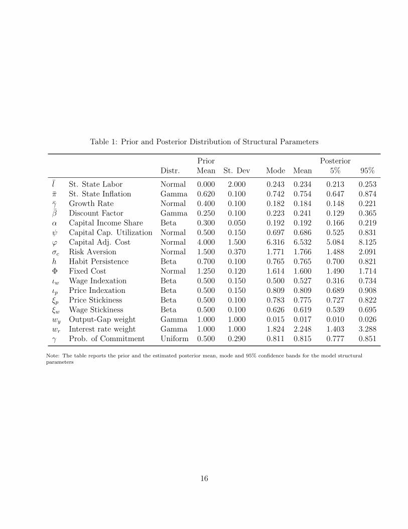
Table 1: Prior and Posterior Distribution of Structural Parameters

Prior PosteriorDistr. Mean St. Dev Mode Mean 5% 95%

l St. State Labor Normal 0.000 2.000 0.243 0.234 0.213 0.253π St. State Inflation Gamma 0.620 0.100 0.742 0.754 0.647 0.874γ Growth Rate Normal 0.400 0.100 0.182 0.184 0.148 0.221β Discount Factor Gamma 0.250 0.100 0.223 0.241 0.129 0.365α Capital Income Share Beta 0.300 0.050 0.192 0.192 0.166 0.219ψ Capital Cap. Utilization Normal 0.500 0.150 0.697 0.686 0.525 0.831ϕ Capital Adj. Cost Normal 4.000 1.500 6.316 6.532 5.084 8.125σc Risk Aversion Normal 1.500 0.370 1.771 1.766 1.488 2.091h Habit Persistence Beta 0.700 0.100 0.765 0.765 0.700 0.821Φ Fixed Cost Normal 1.250 0.120 1.614 1.600 1.490 1.714ιw Wage Indexation Beta 0.500 0.150 0.500 0.527 0.316 0.734ιp Price Indexation Beta 0.500 0.150 0.809 0.809 0.689 0.908ξp Price Stickiness Beta 0.500 0.100 0.783 0.775 0.727 0.822ξw Wage Stickiness Beta 0.500 0.100 0.626 0.619 0.539 0.695wy Output-Gap weight Gamma 1.000 1.000 0.015 0.017 0.010 0.026wr Interest rate weight Gamma 1.000 1.000 1.824 2.248 1.403 3.288γ Prob. of Commitment Uniform 0.500 0.290 0.811 0.815 0.777 0.851

Note: The table reports the prior and the estimated posterior mean, mode and 95% confidence bands for the model structuralparameters

16

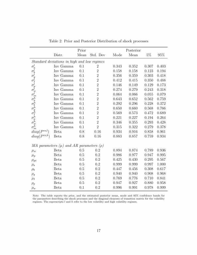
Table 2: Prior and Posterior Distribution of shock processes

Prior PosteriorDistr. Mean Std. Dev Mode Mean 5% 95%

Standard deviations in high and low regimesσla Inv Gamma 0.1 2 0.343 0.352 0.307 0.403σlb Inv Gamma 0.1 2 0.158 0.158 0.123 0.194σlg Inv Gamma 0.1 2 0.356 0.359 0.303 0.418σlI Inv Gamma 0.1 2 0.412 0.415 0.350 0.488σlp Inv Gamma 0.1 2 0.146 0.149 0.129 0.173σlw Inv Gamma 0.1 2 0.274 0.279 0.243 0.318σlm Inv Gamma 0.1 2 0.064 0.066 0.055 0.079σha Inv Gamma 0.1 2 0.643 0.652 0.562 0.759σhb Inv Gamma 0.1 2 0.292 0.296 0.228 0.372σhg Inv Gamma 0.1 2 0.650 0.660 0.568 0.766σhI Inv Gamma 0.1 2 0.569 0.573 0.472 0.689σhp Inv Gamma 0.1 2 0.221 0.227 0.194 0.264σhw Inv Gamma 0.1 2 0.346 0.355 0.293 0.428σhm Inv Gamma 0.1 2 0.315 0.322 0.279 0.378diag(P vo,l) Beta 0.8 0.16 0.934 0.916 0.858 0.961diag(P vo,h) Beta 0.8 0.16 0.883 0.857 0.759 0.934

MA parameters (µ) and AR parameters (ρ)µw Beta 0.5 0.2 0.894 0.874 0.789 0.936µp Beta 0.5 0.2 0.986 0.977 0.947 0.995ρga Beta 0.5 0.2 0.425 0.430 0.295 0.567ρa Beta 0.5 0.2 0.999 0.999 0.997 1.000ρb Beta 0.5 0.2 0.447 0.456 0.308 0.617ρg Beta 0.5 0.2 0.940 0.940 0.908 0.968ρI Beta 0.5 0.2 0.769 0.776 0.710 0.841ρp Beta 0.5 0.2 0.947 0.927 0.880 0.958ρw Beta 0.1 0.2 0.996 0.991 0.978 0.999

Note: The table reports the prior, and the estimated posterior mean, mode and 95% confidence bands forthe parameters describing the shock processes and the diagonal elements of transition matrix for the volatilityregimes. The superscripts l and h refer to the low volatility and high volatility regimes.

17

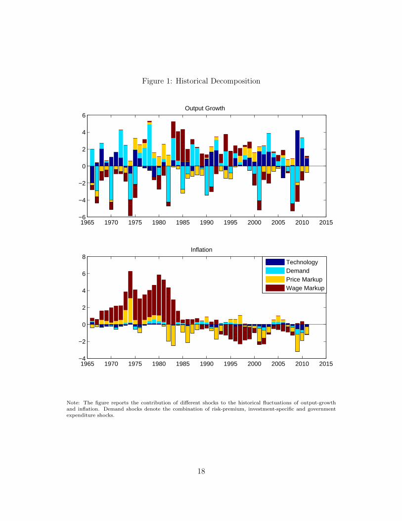
Figure 1: Historical Decomposition

1965 1970 1975 1980 1985 1990 1995 2000 2005 2010 2015−6

−4

−2

0

2

4

6Output Growth

1965 1970 1975 1980 1985 1990 1995 2000 2005 2010 2015−4

−2

0

2

4

6

8Inflation

TechnologyDemandPrice MarkupWage Markup

Note: The figure reports the contribution of different shocks to the historical fluctuations of output-growthand inflation. Demand shocks denote the combination of risk-premium, investment-specific and governmentexpenditure shocks.

18

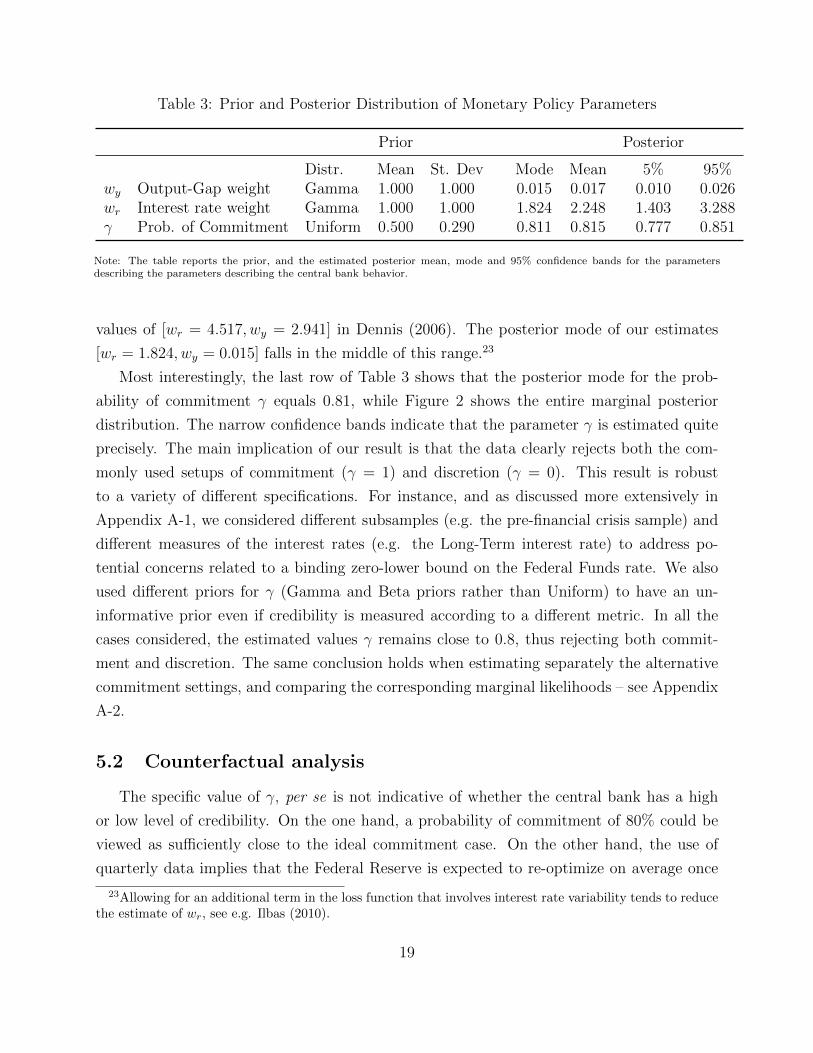
Table 3: Prior and Posterior Distribution of Monetary Policy Parameters

Prior Posterior

Distr. Mean St. Dev Mode Mean 5% 95%wy Output-Gap weight Gamma 1.000 1.000 0.015 0.017 0.010 0.026wr Interest rate weight Gamma 1.000 1.000 1.824 2.248 1.403 3.288γ Prob. of Commitment Uniform 0.500 0.290 0.811 0.815 0.777 0.851

Note: The table reports the prior, and the estimated posterior mean, mode and 95% confidence bands for the parametersdescribing the parameters describing the central bank behavior.

values of [wr = 4.517, wy = 2.941] in Dennis (2006). The posterior mode of our estimates

[wr = 1.824, wy = 0.015] falls in the middle of this range.23

Most interestingly, the last row of Table 3 shows that the posterior mode for the prob-

ability of commitment γ equals 0.81, while Figure 2 shows the entire marginal posterior

distribution. The narrow confidence bands indicate that the parameter γ is estimated quite

precisely. The main implication of our result is that the data clearly rejects both the com-

monly used setups of commitment (γ = 1) and discretion (γ = 0). This result is robust

to a variety of different specifications. For instance, and as discussed more extensively in

Appendix A-1, we considered different subsamples (e.g. the pre-financial crisis sample) and

different measures of the interest rates (e.g. the Long-Term interest rate) to address po-

tential concerns related to a binding zero-lower bound on the Federal Funds rate. We also

used different priors for γ (Gamma and Beta priors rather than Uniform) to have an un-

informative prior even if credibility is measured according to a different metric. In all the

cases considered, the estimated values γ remains close to 0.8, thus rejecting both commit-

ment and discretion. The same conclusion holds when estimating separately the alternative

commitment settings, and comparing the corresponding marginal likelihoods – see Appendix

A-2.

5.2 Counterfactual analysis

The specific value of γ, per se is not indicative of whether the central bank has a high

or low level of credibility. On the one hand, a probability of commitment of 80% could be

viewed as sufficiently close to the ideal commitment case. On the other hand, the use of

quarterly data implies that the Federal Reserve is expected to re-optimize on average once

23Allowing for an additional term in the loss function that involves interest rate variability tends to reducethe estimate of wr, see e.g. Ilbas (2010).

19

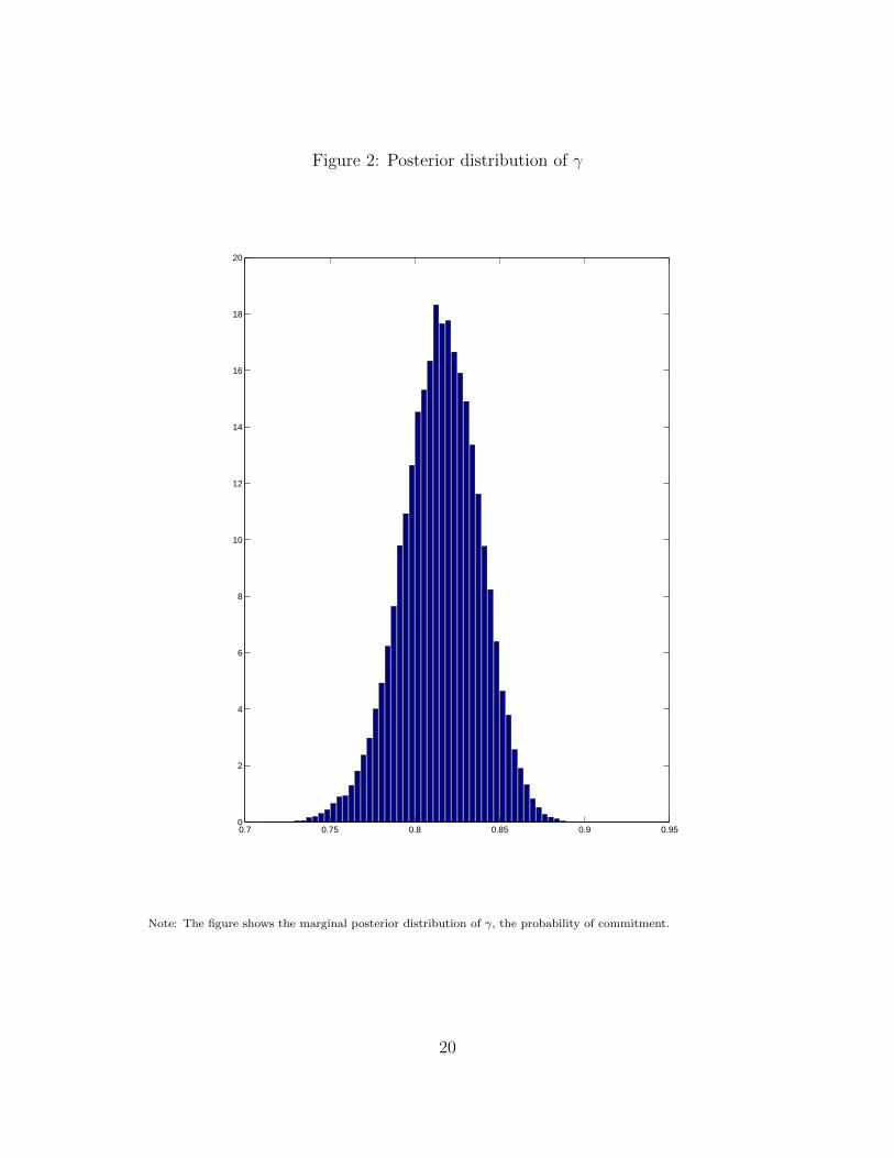
Figure 2: Posterior distribution of γ

0.7 0.75 0.8 0.85 0.9 0.950

2

4

6

8

10

12

14

16

18

20

Note: The figure shows the marginal posterior distribution of γ, the probability of commitment.

20

every 5-quarters, arguably a relatively short commitment horizon.

However, counterfactual exercises can shed light on the nature of our results. The main

question we ask is what would happen under alternative commitment scenarios. To that end

we perform counterfactual simulations of the model assuming that the central bank operates

either under commitment (γ = 1) or under discretion (γ = 0). The remaining parameters of

the model are left unchanged.

Table 4 shows how commitment affects the unconditional second moments for some rel-

evant variables. In general, the relative standard deviations and the cross-correlations with

output in a model with γ = .81 are closer to the discretion than to the commitment case.

The last line of the table also reports the implied welfare losses with respect to the com-

mitment case, measured in terms of equivalent permanent increase in the inflation rate.24

According to that measure, the total gains of passing from discretion to commitment are

equivalent to a permanent decrease in the inflation rate of 1.2% per year. Most of those

gains – corresponding to a 1% permanent reduction in inflation – could still be achieved if

increasing credibility from .081 to 1. We can thus conclude that the economy would behave

quite differently if the central bank had perfect commitment, and thus there is still some

scope to improve credibility.

Next we look at counterfactual paths of inflation and output growth within our sample

period under the assumption of discretion and commitment. The structural shocks are

fixed at the values estimated under the loose commitment setting (i.e., the baseline model).

Figure 3 displays these counterfactual paths. For output growth, both the counterfactuals

under commitment and discretion do not display big differences compared to the data. For

inflation, in the period from the mid-1970s to early-1980s the counterfactual under discretion

is closer to the data. Inflation under commitment is lower during this period, but not low

enough to conclude that the Federal Reserve acting under commitment could have avoided

the ”Great Inflation” of the 1970s. On the contrary, since the early-1980s we see that

the commitment counterfactual path tracks the inflation data almost perfectly . Under

discretion, inflation would have been more volatile, especially so in the past decade. Our

exercise thus suggests that starting from the early 1980s the Federal Reserve behaved very

similarly to a perfectly committed central bank, and that commitment largely contributed

to reduce inflation fluctuations.

More generally, these counterfactual exercises further confirm the idea that the dynamics

24Such a measure is often used to gauge losses for the objective functions employed by central banks andis described, for instance, in Jensen (2002).

21

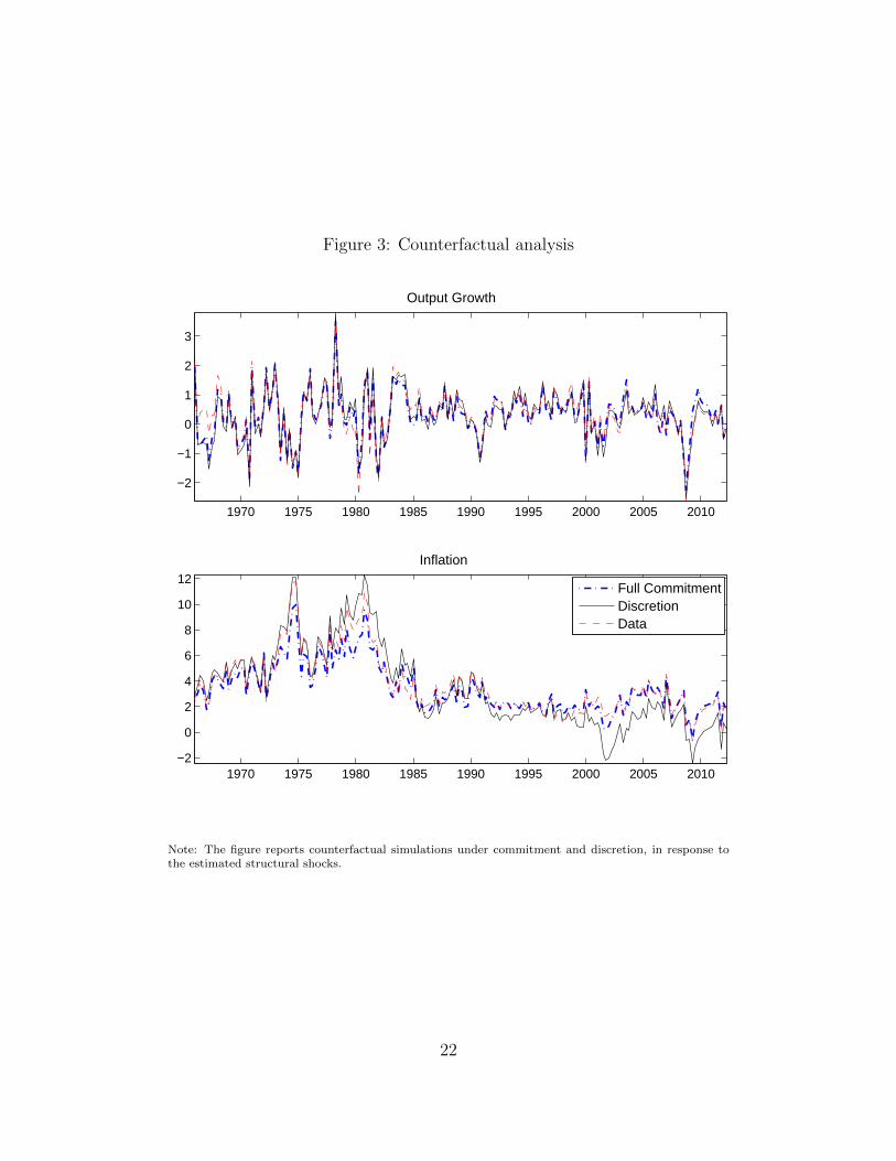
Figure 3: Counterfactual analysis

1970 1975 1980 1985 1990 1995 2000 2005 2010

−2

−1

0

1

2

3

Output Growth

1970 1975 1980 1985 1990 1995 2000 2005 2010−2

0

2

4

6

8

10

12

Inflation

Full CommitmentDiscretionData

Note: The figure reports counterfactual simulations under commitment and discretion, in response tothe estimated structural shocks.

22

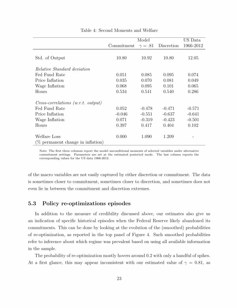
Table 4: Second Moments and Welfare

Model US DataCommitment γ = .81 Discretion 1966-2012

Std. of Output 10.80 10.92 10.80 12.05

Relative Standard deviationFed Fund Rate 0.051 0.085 0.095 0.074Price Inflation 0.035 0.070 0.081 0.049Wage Inflation 0.068 0.095 0.101 0.065Hours 0.534 0.541 0.540 0.286

Cross-correlations (w.r.t. output)Fed Fund Rate 0.052 -0.478 -0.471 -0.571Price Inflation -0.046 -0.551 -0.637 -0.641Wage Inflation 0.071 -0.319 -0.423 -0.501Hours 0.397 0.417 0.404 0.102

Welfare Loss 0.000 1.090 1.209 -(% permanent change in inflation)

Note: The first three columns report the model unconditional moments of selected variables under alternativecommitment settings. Parameters are set at the estimated posteriod mode. The last column reports thecorresponding values for the US data 1966-2012.

of the macro variables are not easily captured by either discretion or commitment. The data

is sometimes closer to commitment, sometimes closer to discretion, and sometimes does not

even lie in between the commitment and discretion extremes.

5.3 Policy re-optimizations episodes

In addition to the measure of credibility discussed above, our estimates also give us

an indication of specific historical episodes when the Federal Reserve likely abandoned its

commitments. This can be done by looking at the evolution of the (smoothed) probabilities

of re-optimization, as reported in the top panel of Figure 4. Such smoothed probabilities

refer to inference about which regime was prevalent based on using all available information

in the sample.

The probability of re-optimization mostly hovers around 0.2 with only a handful of spikes.

At a first glance, this may appear inconsistent with our estimated value of γ = 0.81, as

23

one would expect that the probability of re-optimization should be close to one 20% of

the time, and close to zero the remaining 80%. However, this does not happen in our

model for two reasons. First, in our model γ not only governs the switching re-optimization

variable, but it also affects the expectations regarding the endogenous state variables in

equation 4. The fact the there are fewer re-optimizations episodes than suggested by the

unconditional probability could then reflect the separate roles played by “beliefs” about

credibility (affecting expectations), and actual re-optimizations. Second, and as illustrated

in Section 4, our model identifies re-optimization episodes when there are large differences

in the path of variables with or without re-optimizations xt − xreopt .25 If such difference is

small, as it would be cases during prolonged periods with moderate fluctuations, it would

be almost impossible to distinguish re-optimizations from continuations of past plans. In

such cases, the smoothed probability remains at the unconditional average, i.e. at a level of

about 0.2.

We can isolate five dates when re-optimizations were more likely than continuations

of previous plans – i.e. the probability of re-optimization exceeds 50%. Those dates are

(i) 1969:Q4, (ii) 1980:Q3, (iii) 1984:Q4, (iv) 1989:3 and (v) 2008:Q3. If we lower the cutoff

threshold to 40% then we get two additional dates (vi) 1979:Q1 and (vii) 1993:Q1. A natural

test for the validity of our results is to contrast these dates with existing narrative accounts of

the US monetary policy history. The first two episodes coincide with the appointment of new

Federal Reserve Chairmen: Arthur Burns in early 1970 and Paul Volcker in mid 1979. In late

1980 there is another re-optimization, corresponding to a view that there has been a policy-

reversal during 1980, and that the Volcker policy was credible and effective only from late

1980 or early 1981 (see e.g. Goodfriend and King (2005)). We see another re-optimization

in 1984 which could potentially correspond to the end of the experiment of targeting non-

borrowed reserves that was undertaken in the first few years under Volcker. Only two episodes

are identified over the 20-year long Greenspan tenure. A first re-optimization occurred in

1989, close to the “Romer and Romer” date of December 1988 (see Romer and Romer

(1989)). A second re-optimization is identified in 1993. Arguably, this could be related with

the major policy change of February 1994 when the Federal Reserve began explicitly releasing

its target for the federal funds rate, along with statements of the committee’s opinion on

the direction of the economy. Those announcements were intended to convey information

about future policies, as an additional tool to influence current economic outcomes. The

25For instance, Figure 8 shows those differences for output growth, inflation and the Fed Funds rate, whilethe estimation procedure entails accounting for this difference for all the seven observables.

24

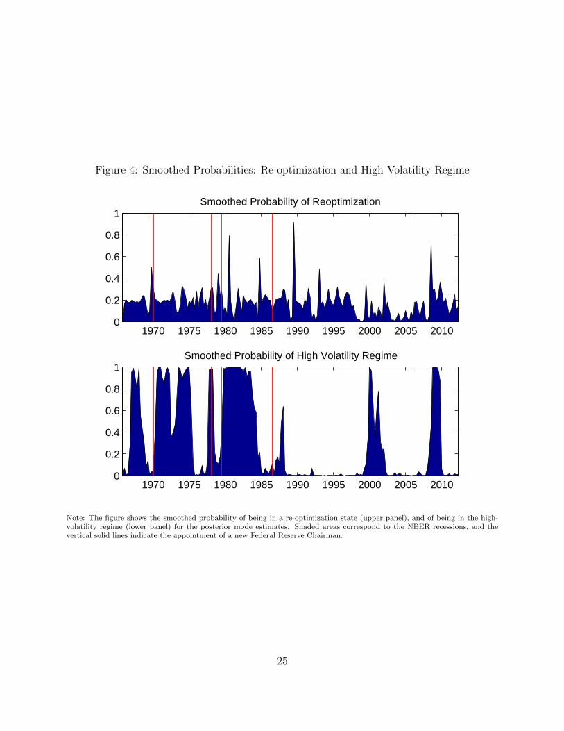
Figure 4: Smoothed Probabilities: Re-optimization and High Volatility Regime

1970 1975 1980 1985 1990 1995 2000 2005 20100

0.2

0.4

0.6

0.8

1Smoothed Probability of Reoptimization

1970 1975 1980 1985 1990 1995 2000 2005 20100

0.2

0.4

0.6

0.8

1Smoothed Probability of High Volatility Regime

Note: The figure shows the smoothed probability of being in a re-optimization state (upper panel), and of being in the high-volatility regime (lower panel) for the posterior mode estimates. Shaded areas correspond to the NBER recessions, and thevertical solid lines indicate the appointment of a new Federal Reserve Chairman.

25

last re-optimization is identified in 2008, when the Federal Reserve started adopting unusual

policy decisions like the purchases of mortgage-backed securities and other long-term financial

assets. Thus overall it appears that some of our dates align with changes in Federal Reserve

chairmen while others correspond to changes in operating procedures of the Federal Reserve.

Moreover, there does not seem to be any systematic correspondence between re-optimizations

and recessions, or switches in the volatility regime. This can be seen in the bottom panel of

figure 4, showing the smoothed probabilities of being in a high volatility regime. The iden-

tified periods of high-volatility are consistent with canonical analyses of US business-cycles,

but are not aligned with our re-optimization episodes. The 70s and the early 80s are char-

acterized by long and recurrent episodes of high-volatility. The probability of high-volatility

surges in correspondence with well-known oil shock episodes: the OPEC oil embargo of 1973-

1974, the Iranian revolution of 1978-1979 and Iran-Iraq war initiated in 1980.26 From 1984

onwards, the economy entered a long period with low-volatility – the Great-Moderation –

interrupted by the bursting of the dot-com bubble in 2000, and by the events in the after-

math of September 11, 2001. Finally, periods with high-volatility are clearly identified in

correspondence with the Great-Recession and financial crisis of 2008-2009.

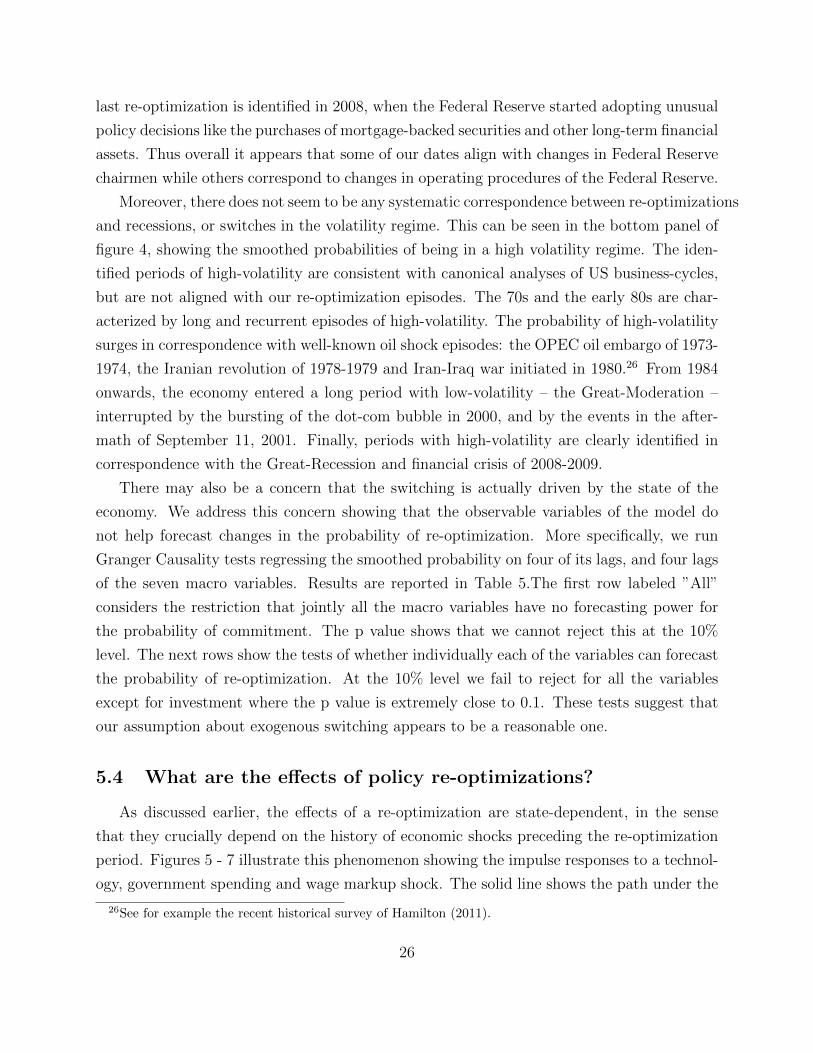
There may also be a concern that the switching is actually driven by the state of the

economy. We address this concern showing that the observable variables of the model do

not help forecast changes in the probability of re-optimization. More specifically, we run

Granger Causality tests regressing the smoothed probability on four of its lags, and four lags

of the seven macro variables. Results are reported in Table 5.The first row labeled ”All”

considers the restriction that jointly all the macro variables have no forecasting power for

the probability of commitment. The p value shows that we cannot reject this at the 10%

level. The next rows show the tests of whether individually each of the variables can forecast

the probability of re-optimization. At the 10% level we fail to reject for all the variables

except for investment where the p value is extremely close to 0.1. These tests suggest that

our assumption about exogenous switching appears to be a reasonable one.

5.4 What are the effects of policy re-optimizations?

As discussed earlier, the effects of a re-optimization are state-dependent, in the sense

that they crucially depend on the history of economic shocks preceding the re-optimization

period. Figures 5 - 7 illustrate this phenomenon showing the impulse responses to a technol-

ogy, government spending and wage markup shock. The solid line shows the path under the

26See for example the recent historical survey of Hamilton (2011).

26

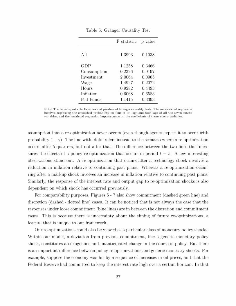
Table 5: Granger Causality Test

F statistic p value

All 1.3993 0.1038

GDP 1.1258 0.3466Consumption 0.2326 0.9197Investment 2.0064 0.0965Wage 1.4927 0.2072Hours 0.9282 0.4493Inflation 0.6068 0.6583Fed Funds 1.1415 0.3393

Note: The table reports the F-values and p-values of Granger causality tests. The unrestricted regressioninvolves regressing the smoothed probability on four of its lags and four lags of all the seven macrovariables, and the restricted regression imposes zeros on the coefficients of those macro variables.

assumption that a re-optimization never occurs (even though agents expect it to occur with

probability 1−γ). The line with ‘dots’ refers instead to the scenario where a re-optimization

occurs after 5 quarters, but not after that. The difference between the two lines thus mea-

sures the effects of a policy re-optimization that occurs in period t = 5. A few interesting

observations stand out. A re-optimization that occurs after a technology shock involves a

reduction in inflation relative to continuing past plans. Whereas a re-optimization occur-

ring after a markup shock involves an increase in inflation relative to continuing past plans.

Similarly, the response of the interest rate and output gap to re-optimization shocks is also

dependent on which shock has occurred previously.

For comparability purposes, Figures 5 - 7 also show commitment (dashed green line) and

discretion (dashed - dotted line) cases. It can be noticed that is not always the case that the

responses under loose commitment (blue lines) are in between the discretion and commitment

cases. This is because there is uncertainty about the timing of future re-optimizations, a

feature that is unique to our framework.

Our re-optimizations could also be viewed as a particular class of monetary policy shocks.

Within our model, a deviation from previous commitment, like a generic monetary policy

shock, constitutes an exogenous and unanticipated change in the course of policy. But there

is an important difference between policy re-optimizations and generic monetary shocks. For

example, suppose the economy was hit by a sequence of increases in oil prices, and that the

Federal Reserve had committed to keep the interest rate high over a certain horizon. In that

27

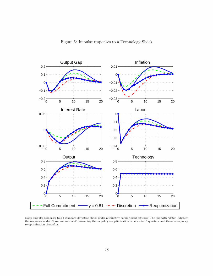
Figure 5: Impulse responses to a Technology Shock

0 5 10 15 20−0.2

−0.1

0

0.1

0.2Output Gap

0 5 10 15 20−0.03

−0.02

−0.01

0

0.01Inflation

0 5 10 15 20−0.05

0

0.05Interest Rate

0 5 10 15 20−0.4

−0.3

−0.2

−0.1

0Labor

0 5 10 15 200

0.2

0.4

0.6

0.8Output

0 5 10 15 200

0.2

0.4

0.6

0.8Technology

Full Commitment γ = 0.81 Discretion Reoptimization

Note: Impulse responses to a 1 standard deviation shock under alternative commitment settings. The line with “dots” indicatesthe responses under “loose commitment”, assuming that a policy re-optimization occurs after 5 quarters, and there is no policyre-optimization thereafter.

28

Figure 6: Impulse responses to a Demand Shock

0 5 10 15 20−0.1

0

0.1

0.2

0.3Output Gap

0 5 10 15 20−0.01

0

0.01

0.02Inflation

0 5 10 15 20−0.02

0

0.02

0.04

0.06Interest Rate

0 5 10 15 200

0.1

0.2

0.3

0.4Labor

0 5 10 15 20−0.2

0

0.2

0.4

0.6Output

0 5 10 15 200

0.2

0.4

0.6

0.8Govt. Exp.

Full Commitment γ = 0.81 Discretion Reoptimization

Note: Impulse responses to a 1 standard deviation government expenditure shock under alternative commitment settings. Theline with “dots” indicates the responses under “loose commitment”, assuming that a policy re-optimization occurs after 5quarters, and there is no policy re-optimization thereafter.

29

Figure 7: Impulse responses to a Wage-Markup Shock

0 5 10 15 20−6

−4

−2

0Output Gap

0 5 10 15 20−0.2

0

0.2

0.4

0.6Inflation

0 5 10 15 20−0.2

0

0.2

0.4

0.6Interest Rate

0 5 10 15 20−3

−2

−1

0Labor

0 5 10 15 20−6

−4

−2

0Output

0 5 10 15 200

0.5

1sw

Full Commitment γ = 0.81 Discretion Reoptimization

Note: Impulse responses to a 1 standard deviation wage markup shock under alternative commitment settings. The line with“dots” indicates the responses under “loose commitment”, assuming that a policy re-optimization occurs after 5 quarters, andthere is no policy re-optimization thereafter.

30

case, a policy re-optimization would bring about more expansionary policy than expected.

On the contrary, in an economy affected by negative demand shocks, the central bank would

commit to keep the interest rate low, and and a re-optimization would then be associated

with an unanticipated contractionary policy. Thus, whether a re-optimization has a positive

or a negative impact on the variables of interest depends on the entire sequence of shocks

previously experienced by the economy.

It then seems useful to analyze the effects of re-optimizations over our sample period. To

that end, figure 8 illustrates the effects of deviating from a promised plan on a given date.

Specifically it shows the difference, [xt|st = 0, xt−1] − [xt|st = 1, xt−1] for output growth,

inflation and the nominal interest rate. The thought experiment is the following: if a re-

optimization were to occur at each period in our sample, how would the values of output,

inflation and interest rates be different relative to the case where the previous commitment

is honored?27 Policy re-optimizations would have made output and inflation higher until

the early 1980s, but would have had a negligible effect (or lowered them) during the Great

Moderation. This is because in periods with high volatility the central bank needs to make

significant commitments to its future actions to stabilize the economy. Those commitments

constitute a relevant burden in subsequent periods, and abandoning past commitment would

lead to a radically different outcomes. Instead, in a low volatility economy the central bank

carries over less relevant commitments, and there is less need to stabilize the economy. As a

consequence, the effects of abandoning past commitments are relatively small.

Regarding the episodes discussed above, Figure 8 shows that the re-optimizations of

the ’70s and ’80s are all associated with an increase in the level of inflation and output

growth. In other words, those re-optimizations implied a “looser” policy than under the

commitment plan. The two re-optimizations of 1993 and 2009 are instead associated with

a more contractionary policy. This suggests that Quantitative Easing does constitute a

deviation from a commitment plan, but in the sense that monetary policy should have been

more expansionary than it actually was. This conforms to the common view that as the

economy hit the zero-lower bound, quantitative easing was a necessary but insufficient tool.

27Keep in mind that this exercise is conducted conditioning on the estimated parameters being consistentwith an unconditional probability of commitment being equal to our estimated value of 0.81.

31

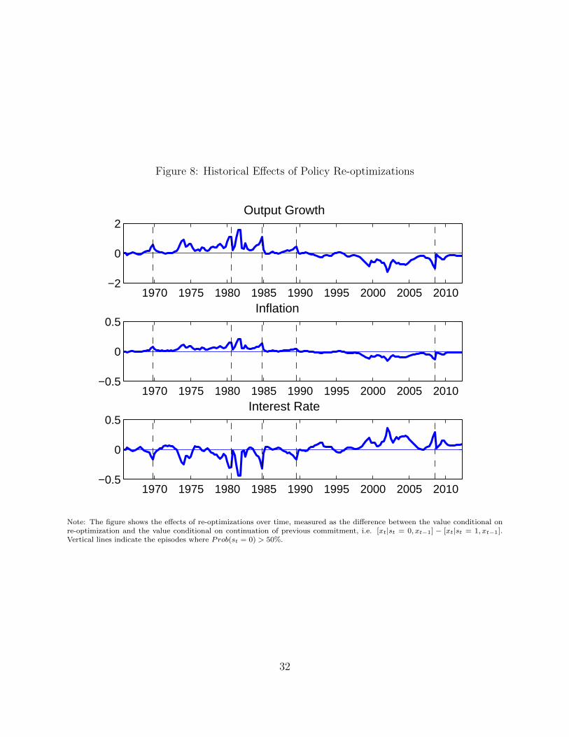
Figure 8: Historical Effects of Policy Re-optimizations

1970 1975 1980 1985 1990 1995 2000 2005 2010−2

0

2Output Growth

1970 1975 1980 1985 1990 1995 2000 2005 2010−0.5

0

0.5Inflation

1970 1975 1980 1985 1990 1995 2000 2005 2010−0.5

0

0.5Interest Rate

Note: The figure shows the effects of re-optimizations over time, measured as the difference between the value conditional onre-optimization and the value conditional on continuation of previous commitment, i.e. [xt|st = 0, xt−1] − [xt|st = 1, xt−1].Vertical lines indicate the episodes where Prob(st = 0) > 50%.

32

6 Conclusion

This paper proposes a structural econometric approach to measure the degree of the Fed-

eral Reserve’s credibility, within a standard medium-scale macroeconomic model. Monetary

policy choices are modeled according to a loose commitment setting, where deviations from

commitment plans are governed by a regime-switching process.

The conventional approach to think about central banks’ credibility is to distinguish

between two polar cases: commitment and discretion. Our results depict a very different

picture regarding the actual behavior of the Federal Reserve. Over the past four decades,

the Fed displayed a certain ability to commit, but its credibility was not perfect. There have

been periods where the Fed honored its commitments, but also episodes when it did not.

Such episodes sometimes line up closely with changes of Fed chairmen, and other times with

changes in the operational procedures of the Federal Reserve.

Moreover, counterfactual exercises show that the behavior of the Federal has changed

over time. During the ’70s, the actual inflation dynamics would indicate a discretionary

behavior. Instead, starting from the mid 1980s inflation dynamics are more consistent with

a commitment behavior. But it would be misleading to conclude that there has been a one-

time change from discretion to commitment. The Federal Reserve has occasionally deviated

from its commitment plans throughout the entire sample. If anything, the main difference

is that while the deviations in the 70’s implied more expansionary policies, the deviations in

the 90’s and 2000’s has been more contractionary. In this respect, our result are consistent

with earlier studies in the monetary policy literature arguing that the Fed moved from a

passive to an active regime, and the associated “good policies” contributed to the Great

-Moderation.

According to our model, there is still some scope to increase the credibility of the Fed-

eral Reserve. Credibility gains would reduce the fluctuations in measures of inflation and

economic activity, and thus enhance welfare. Our study, however, remains silent about the

specific sources of credibility problems, and thus on the possible ways to correct them. For

instance, under the helm of chairman Ben Bernanke, the Federal Reserve has taken several

measures to better communicate with the public about current and future policy actions.

In 2012 the Federal Reserve announced an official inflation target of 2%. Additionally they

started releasing individual forecasts of the FOMC members’ relating to economic activity.

Looking forward, our approach could be used to assess the effectiveness of these type of

policies.

33

References

Adolfson, M., S. Laseen, J. Linde, and L. E. Svensson (2011, October). Optimal mone-

tary policy in an operational medium sized dsge model. Journal of Money, Credit and

Banking 43 (7), 1287–1331.

Backus, D. and J. Driffill (1985). Inflation and reputation. American Economic Review 75 (3),

530–38.

Barro, R. J. and D. B. Gordon (1983). Rules, discretion and reputation in a model of

monetary policy. Journal of Monetary Economics 12 (1), 101–121.

Benigno, P. and M. Woodford (2012). Linear-quadratic approximation of optimal policy

problems. Journal of Economic Theory 147 (1), 1 – 42.

Berger, H. and U. Woitek (2005). Does conservatism matter? a time-series approach to

central bank behaviour. Economic Journal 115 (505), 745–766.

Bianchi, F. (2012). Regime switches, agents’ beliefs, and post-world war ii u.s. macroeco-

nomic dynamics*. The Review of Economic Studies .

Blinder, A. S. (2000, December). Central-bank credibility: Why do we care? how do we

build it? American Economic Review 90 (5), 1421–1431.

Chappell, H., T. Havrilesky, and R. McGregor (1993). Partisan monetary policies: Pres-

idential influence through the power of appointment. The Quarterly Journal of Eco-

nomics 108 (1), 185–218.

Chen, X., T. Kirsanova, and C. Leith (2013). How optimal is us monetary policy? Technical

report, University of Glasgow.

Chib, S. and S. Ramamurthy (2010). Tailored randomized block {MCMC} methods with

application to {DSGE} models. Journal of Econometrics 155 (1), 19 – 38.

Clarida, R., J. Galı, and M. Gertler (1999). The science of monetary policy: A new keynesian

perspective. Journal of Economic Literature 37 (4), 1661–1707.

Cogley, T. and T. J. Sargent (2006). Drifts and volatilities: Monetary policies and outcomes

in the post wwii u.s. Review of Economic Dynamics 8, 262–232.

34

Coroneo, L., V. Corradi, and P. S. Monteiro (2013). Testing for optimal monetary policy via

moment inequalities. Technical report, University of York.

Cukierman, A. (1992). Central bank strategy, credibility, and independence: Theory and

evidence. MIT Press Books 1.

Davig, T. and E. Leeper (2007). Generalizing the taylor principle. American Economic

Review 97 (3), 607–635.

Debortoli, D., J. Maih, and R. Nunes (2012, 7). Loose commitment in medium-scale macroe-

conomic models: Theory and applications. Macroeconomic Dynamics FirstView, 1–24.

Debortoli, D. and R. Nunes (2010, May). Fiscal policy under loose commitment. Journal of

Economic Theory 145 (3), 1005–1032.

Debortoli, D. and R. Nunes (2013). Monetary regime-switches and central bank’s preferences.

Technical report, University of California San Diego.

Dennis, R. (2004, September). Inferring policy objectives from policy actions. Oxford Bulletin

of Economics and Statistics 66, 745–764.

Dennis, R. (2006). The policy preferences of the us federal reserve. Journal of Applied

Econometrics 21 (1), 55–77.

Dennis, R. (2007, February). Optimal policy in rational expectations models: New solution

algorithms. Macroeconomic Dynamics 11 (01), 31–55.

Erceg, C. J., D. W. Henderson, and A. T. Levin (2000). Optimal monetary policy with

staggered wage and price contracts. Journal of Monetary Economics 46 (2), 281–313.

Farmer, R. E., D. F. Waggoner, and T. Zha (2009). Understanding markov-switching rational

expectations models. Journal of Economic Theory 144 (5), 1849–1867.

Favero, C. A. and R. Rovelli (2003). Macroeconomic stability and the preferences of the fed:

A formal analysis, 1961–98. Journal of Money, Credit and Banking 35 (4), 545 – 556.

Gamerman, D. and H. F. Lopes (2006). Markov chain Monte Carlo: stochastic simulation

for Bayesian inference, Volume 68. Chapman & Hall/CRC.

35

Gelfand, A. E. and D. K. Dey (1994). Bayesian model choice: Asymptotics and exact

calculations. Journal of the Royal Statistical Society. Series B (Methodological) 56 (3), pp.

501–514.

Geweke, J. (1992). Evaluating the accuracy of sampling-based approaches to the calculation

of posterior moments. In In Bayesian Statistics, pp. 169–193. University Press.

Geweke, J. (1999). Using simulation methods for bayesian econometric models: inference,

development,and communication. Econometric Reviews 18 (1), 1–73.

Givens, G. E. (2012, 09). Estimating central bank preferences under commitment and dis-

cretion. Journal of Money, Credit and Banking 44 (6), 1033–1061.

Goodfriend, M. and R. G. King (2005, July). The incredible volcker disinflation. Journal of

Monetary Economics 52 (5), 981–1015.

Gurkaynak, R., B. Sack, and E. Swanson (2005, March). The sensitivity of long-term interest

rates to economic news: Evidence and implications for macroeconomic models. American

Economic Review 95 (1), 425–436.

Hamilton, J. D. (1989). A new approach to the economic analysis of nonstationary time

series and the business cycle. Econometrica, 357–384.

Hamilton, J. D. (2011, February). Historical oil shocks. NBER Working Papers 16790,

National Bureau of Economic Research, Inc.

Havrilesky, T. (1995). The Pressures on American Monetary Policy. Kluwer Academic

Publishers.

Ilbas, P. (2010). Revealing the preferences of the us federal reserve. Journal of Applied

Econometrics .

Jensen, H. (2002). Targeting nominal income growth or inflation? American Economic

Review 92 (4), 928–956.

Justiniano, A. and G. E. Primiceri (2008, June). The time-varying volatility of macroeco-

nomic fluctuations. American Economic Review 98 (3), 604–41.

Kara, A. H. (2007, March). Monetary policy under imperfect commitment: Reconciling

theory with evidence. International Journal of Central Banking , 149–177.

36

Kim, C.-J. and C. R. Nelson (1999). State-Space Models with Regime Switching: Classical

and Gibbs-Sampling Approaches with Applications, Volume 1 of MIT Press Books. The

MIT Press.

Kimball, M. S. (1995). The quantitative analytics of the basic neomonetarist model. Journal

of Money, Credit and Banking 27 (4), 1241–77.

Kydland, F. E. and E. C. Prescott (1977). Rules rather than discretion: The inconsistency

of optimal plans. Journal of Political Economy 85 (3), 473–91.

Kydland, F. E. and E. C. Prescott (1980). Dynamic optimal taxation, rational expectations

and optimal control. Journal of Economic Dynamics and Control 2(1), 79–91.

Lakdawala, A. (2013). Changes in federal reserve preferences. Michigan State University,

Working Paper .

Liu, Z., D. F. Waggoner, and T. Zha (2011). Sources of macroeconomic fluctuations: A

regime-switching dsge approach. Quantitative Economics 2 (2), 251–301.

Marcet, A. and R. Marimon (2011). Recursive contracts. mimeo, European University

Institute.

Mishkin, F. (2009). Monetary Policy Strategy. MIT press.

Primiceri, G. E. (2005). Time varying structural vector autoregressions and monetary policy.

Review of Economic Studies 72 (3), 821–852.

Roberds, W. (1987). Models of policy under stochastic replanning. International Economic

Review 28 (3), 731–755.

Rogoff, K. (1985). The optimal degree if commitment to an intermediate monetary target.

Quarterly Journal of Economics 100 (4), 1169–89.

Romer, C. D. and D. H. Romer (1989, January). Does monetary policy matter? a new test

in the spirit of friedman and schwartz. In NBER Macroeconomics Annual 1989, Volume

4, NBER Chapters, pp. 121–184. National Bureau of Economic Research, Inc.

Rudebusch, G. and L. E. Svensson (1999). Policy rules for inflation targeting. In Monetary

policy rules, pp. 203–262. University of Chicago Press.

37

Salemi, M. K. (2006, October). Econometric policy evaluation and inverse control. Journal

of Money, Credit and Banking 38 (7), 1737–64.

Schaumburg, E. and A. Tambalotti (2007). An investigation of the gains from commitment

in monetary policy. Journal of Monetary Economics 54 (2), 302–324.

Sims, C. (2002, October). Solving linear rational expectations models. Computational Eco-

nomics 20 (1-2), 1–20.

Sims, C. A. and T. Zha (2006). Were there regime switches in u.s. monetary policy? The

American Economic Review 96 (1), 54–81.

Smets, F. and R. Wouters (2007). Shocks and frictions in us business cycles: A bayesian

dsge approach. American Economic Review 97 (3), 586–606.

Soderlind, P. (1999). Solution and estimation of re macromodels with optimal policy. Euro-

pean Economic Review 93, 813–823.

Soderstrom, U., P. Soderlind, and A. Vredin (2005, September 2005). New-keynesian models

and monetary policy: A reexamination of the stylized facts. The Scandinavian Journal of

Economics 107(3), 521–46.

Svensson, L. E. (1999). Inflation targeting as a monetary policy rule. Journal of monetary

economics 43 (3), 607–654.

Svensson, L. E. O. (1994, April). The simplest test of inflation target credibility. CEPR

Discussion Papers 940, C.E.P.R. Discussion Papers.

Walsh, C. E. (1995). Optimal contracts for central bankers. The American Economic Re-

view 85 (1), pp. 150–167.

Yun, T. (1996). Nominal price rigidity, money supply endogeneity and business cycles.

Journal of Monetary Economics 37 (2), 345–370.

38

Appendix

A-1 Robustness Checks

In this section we discuss a variety of robustness checks. Results are summarized in Table

6, where the first column describes how each specification differs from the benchmark case

considered in the main text. For practical purposes, the table only reports the posterior

mode estimates of the policy parameters wy, wr and γ. The complete results are available

upon request to the authors.

To facilitate the comparison, row (a) reports again the benchmark results. Row (b)

contains the estimates excluding data since the beginning of the financial crisis, so that the

data sample is restricted to end at Q2:2007. This is because, we want to make sure that our

main results are not affected by features of the finical crisis that are not explicitly included in

our model, like unconventional policies and the zero-lower bound constraint. The estimates

of γ and wy remain very close to the benchmark case, whereas the estimate of wr is lower at

0.87. This lower estimate is most likely due to the fact that the Federal Reserve has kept the

Fed funds rate constant (around zero) from late 2008 onwards. Similarly, Row (c) shows the

estimates under a specification where the Fed Funds rate is replaced with the interest rate

on a 10-year Treasury note. This allows us to estimate the model using the entire sample

without worrying about the zero lower bound. The resulting estimate of the probability of

commitment is 0.8.

Table 6: Estimates under various specifications

Specification Posterior modewy wr γ

(a) Benchmark 0.015 1.824 0.811(b) Pre-fin crisis sample 0.031 0.874 0.781(c) 10-year interest rate 0.019 1.244 0.803(d) Beta(0.5,0.5) prior for γ 0.015 1.829 0.812(e) Gamma(2,4) prior for wr and wy 0.016 1.950 0.812(f) AR(1) price-markup shocks 0.012 2.009 0.729(g) σl = 0.5 0.022 0.879 0.801(h) σl = 1.92 0.014 1.804 0.812(i) σl = 3 0.022 0.879 0.801

Note: The table shows the posterior mode estimates of the loss function weight on output wy , theloss function weight on interest rate smoothing wr and the probability of commitment γ for variousspecifications.

39

We also consider different prior specifications for the monetary policy parameters. Row

(d) considers a Beta prior for the probability of commitment γ, with both shape parameters

set to 0.5. This prior distribution gives roughly the same weight to values in the [0.2,0.8]

interval while putting more weight on values near the end points 0 and 1. Such specification

confirms that even with a higher prior probability weight on discretion (0) and commitment

(1), the data chooses a value of γ close to 0.8. Row (e) considers Gamma distribution for

wy and wr with a higher variance. Specifically we use the Gamma distribution with mean 2

and variance 4, but the resulting estimates are very similar to the benchmark case.

We then estimate the model allowing for a different specification of the price-markup

process. In the benchmark estimation the price-markup disturbance is modeled as an

ARMA(1,1), εpt = ρpεt−1 + ηpt − µpηpt−1. The estimates from Table 2 show that we have

an issue of near-cancelation of the roots, and potential weak identification. A similar prob-

lem is reported in Justiniano and Primiceri (2008), who end up using an i.i.d. specification.

To ensure the our estimate of the probability of commitment is not affected by this issue,

we consider an additional specification of the price-markup process, where εpt is AR(1). The

results are presented in row (f) of table 6. In this specification the estimate of ρp is very

close to zero, making this very similar to the i.i.d. case of Justiniano and Primiceri (2008).

Importantly, the estimates of γ, wy and wr are not affected much by the specification of the

price-markup process.

Finally, as opposed to the original SW model, in our benchmark estimation we fix the

elasticity of labor supply with respect to the real wage, σl = 1. That parameter displayed

very large confidence bands in the SW estimates, and fixing it improves the convergence

properties of our estimation algorithm.We then consider three alternative values of σl: a

value of 0.5, that is close to what is typically estimated in micro studies; a value of 1.92

corresponding to the posterior mode SW; and a value of 3 that is close to the estimates

in Bianchi (2012) (who estimates a regime-switching model similar to ours). The estimates

of wy and γ (shown in the last 3 rows) are very similar to the benchmark case, while the

estimate of wr does change somewhat (see section 5.1 for a more in-depth discussion of the

sensitivity of this parameter.

In conclusion, the estimate of the probability of commitment γ is stable for all the different

specifications considered.

40

A-2 Comparison of fit of the model

Our model nests both the cases of commitment and discretion, thus the estimated results

imply that the data gives a higher weight to the posterior at γ = .81 as compared to γ = 0

or γ = 1. However a potentially different way to estimate the model at the end points,

γ = 0 or γ = 1, is to use an estimation strategy that does not involve regime-switching

in the coefficient matrices. What we are worried about is the following. Even though the

posterior (and also the likelihood given our diffuse priors) puts a higher weight on γ = .81,

once we take into account the estimation uncertainty involved with the regime-switching, is

it possible that the fit of the discretion or commitment model can be better than the loose

commitment model? To explore this, we separately estimate the commitment and discretion

versions of the model using an estimation strategy that does not involve regime-switching in

the coefficients. There is still regime-switching in the variance of the shocks.

Table 7 shows the marginal likelihoods. These are based on the harmonic mean method

of Gelfand and Dey (1994) and specific one we use is the modified harmonic mean estimator

of Geweke (1999). It is reassuring to see that the fit of the loose commitment model is

significantly better than the discretion case. With commitment, we had difficulty getting

the Bayesian MCMC algorithm to converge. But the posterior mode for commitment is

much lower and we are confident that discretion and loose commitment fit the data much

better than for commitment. See Givens (2012) among others for supporting evidence that

commitment tends to fit the data much worse than discretion.

Finally, we compare our model with the original SW model to compare the fit. For

this exercise the models are estimated stopping the sample before the start of the financial

crisis. We use the original priors used in the SW model, and the baseline priors for the

loose commitment model. The marginal likelihood for our model is higher but not by much.

These marginal likelihood calculations do depend to a small extent on the priors and so

we conclude that our model fits the data at least as well as the SW model, which is the

workhorse model in the literature.

41

Table 7: Comparison of Marginal Likelihhod

Model Data Sample Marginal Likelihood

Discretion Full -1127.69Benchmark Full -1020.36

Smets & Wouters (2007) Pre-fin crisis -880.25Benchmark Pre-fin crisis -874.45

A-3 Details of the Estimation Algorithm

A-3.1 Evaluating the Likelihood Function

Consider the state-space form that can be obtained combining eqs. (2) and (5)

xobst = A+Hβt (1)

βt = Fstβt−1 +Gvt (2)

where βt ≡ [xt, λt]. Also, let’s denote with M the number of possible states the the Markov-

switching process can take. In our case we have 2 states for the policy regimes, and 2 states

for the volatility regimes. Thus, the combined Markov-switching process St ≡ [st, svot ] can

take M = 4 possible values. The likelihood function is evaluated in four steps.

Step 1: Perform the Kalman Filter for i = 1, ..M, j = 1, ..M

βi,jt|t−1 = Fjβit−1|t−1

P i,jt|t−1 = FjP

it−1|t−1F

′j +GQG′

ηi,jt|t−1 = xobst −Hβi,jt|t−1 − Azt

f i,jt|t−1 = HP i,jt|t−1H

′

βi,jt|t = βi,jt|t−1 + P i,jt|t−1H

′[f i,jt|t−1]−1ηi,jt|t−1

P i,jt|t = (I − P i,j

t|t−1H′[f i,jt|t−1]−1H)P i,j

t|t−1

42

Step 2: Perform the Hamilton Filter

P (St, St−1) = P (St|St−1)P (St−1|ψt−1)

f(xobst |ψt−1) =∑St

∑St−1

f(xobst |St, St−1, ψt−1)P (St, St−1|ψt−1)

P (St|ψt) =∑St−1

P (St, St−1|ψt)

Note that the conditional density is normal and given by

f(xobst |St−1 = i, St=j, ψt−1) = (2π)−N2 |f i,jt|t−1|

− 12 exp{−1

2ηi,j

′

t|t−1(f i,jt|t−1)−1ηi,jt|t−1}

Step 3: Perform the Kim & Nelson approximations to collapse the M2 unobservable βi,jt|tinto M ones. For each j calculate the following

βjt|t =

∑Mi=1 P (St = i, St = j|ψt)βi,jt|t

P (St = j|ψt)

P jt|t =

∑Mi=1 P (St = j, St−1 = i|ψt)[P i,j

t|t + (βjt|t − βi,jt|t )(β

jt|t − β

i,jt|t )′]

P (St = j|ψt)

Step 4: After performing steps 1-3 ∀t we can evaluate the log likelihood function

l(θ) =T∑t=1

ln(f(xobst |ψt−1))

A-3.2 Metropolis-Hastings Algorithm

This section explains the Bayesian estimation procedure that uses the Metropolis-Hastings

algorithm and will be used to estimate all the parameters of the model jointly. Our estima-

tion method follows the Metropolis-Hastings algorithm used in SW. The main difference is

that the evaluation of the likelihood has to be modified to deal with the addition of regime-

switching. The estimation follows a two step procedure. In the first step we numerically

maximize the log posterior distribution to get an estimate of the posterior mode. In the

second step, using the posterior mode calculated in the first step as a starting value, we use

the Metropolis-Hastings algorithm to completely characterize the posterior distribution.

Let θ be the parameters to be estimated. The M-H algorithm involves generating a draw

from a candidate generating density, q(.). Given a draw θ(g), let the candidate draw be called

43

θ(g+1). Then this new draw is accepted with the following probability.

α(θ(g+1), θ(g)) = min

(p(θ(g+1)|Y ).q(θ(g))

p(θ(g)|Y ).q(θ(g+1)), 1

)Following SW(2007) we use the inverse of the Hessian at the posterior mode (that comes

out of the numerical optimization procedure) in the candidate generating density which is

centered around the current draw δ(g).

δ(g+1) = δ(g) + cH−1

where c is a scale factor and H is the Hessian at the posterior mode. This is known as a

random walk Metropolis-Hastings step. We then tune the parameter c to get an acceptance

rate of between 25% and 35% as recommended by Gamerman and Lopes (2006). The full

parameter vector θ is sampled in one block. We have also tried blocking by splitting the

parameter vector θ into 2 or more blocks but found that the Metropolis-Hastings algorithm

ran most efficiently with one block and had good convergence properties as discussed below.

A-3.3 Convergence Diagnostics

The Metropolis-Hastings algorithm is run for 500,000 draws where the first 25,000 draws

are discarded. Note since the chain is initialized at the posterior mode, a large number of

burn-in draws is not required. From the remaining 475,000 draws, one of out of every ten

draws is saved resulting in an effective sample of 47,500. Figure 9 shows the trace plots of

the draws from the Metropolis-Hastings algorithm for the three structural parameters that

are new to our setting. As can be seen the draws are mixing well. To get a better idea of

the correlation of the draws the top panel of figure 10 plots the 20th order autocorrelation

for each of the estimated parameters. These autocorrelations are all below 0.6 and most

them lower than 0.3, suggesting that the dependence in the draws diminishes fairly rapidly.

The lower panel shows the inefficiency factors, this is the inverse of the relative numerical

efficiency of Geweke (1992). These numbers are mostly below 40 while some of them are a

bit higher. Note these are much lower as compared to the SW M-H algorithm as reported by

Chib and Ramamurthy (2010). Thus, overall the convergence diagnostics are satisfactory.

44

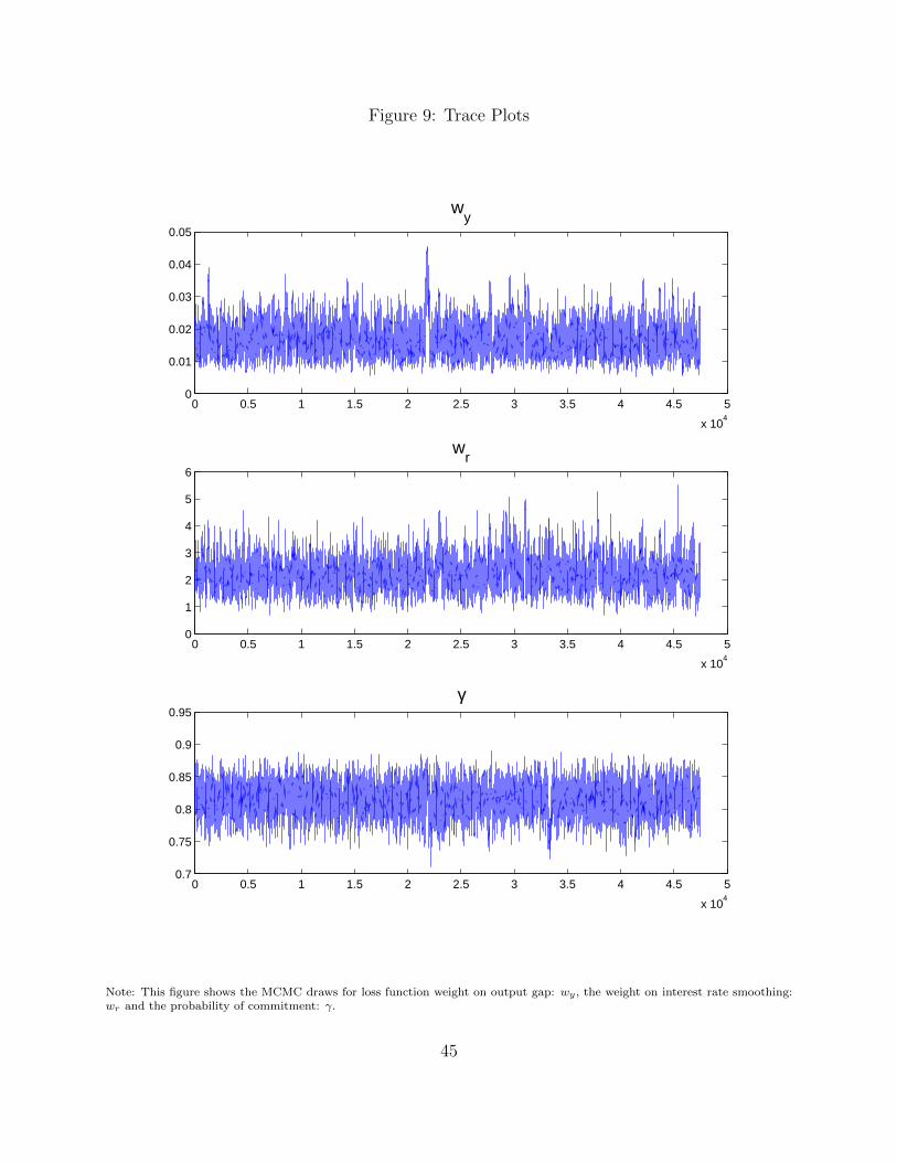
Figure 9: Trace Plots

0 0.5 1 1.5 2 2.5 3 3.5 4 4.5 5

x 104

0

0.01

0.02

0.03

0.04

0.05

wy

0 0.5 1 1.5 2 2.5 3 3.5 4 4.5 5

x 104

0

1

2

3

4

5

6

wr

0 0.5 1 1.5 2 2.5 3 3.5 4 4.5 5

x 104

0.7

0.75

0.8

0.85

0.9

0.95γ

Note: This figure shows the MCMC draws for loss function weight on output gap: wy , the weight on interest rate smoothing:wr and the probability of commitment: γ.

45

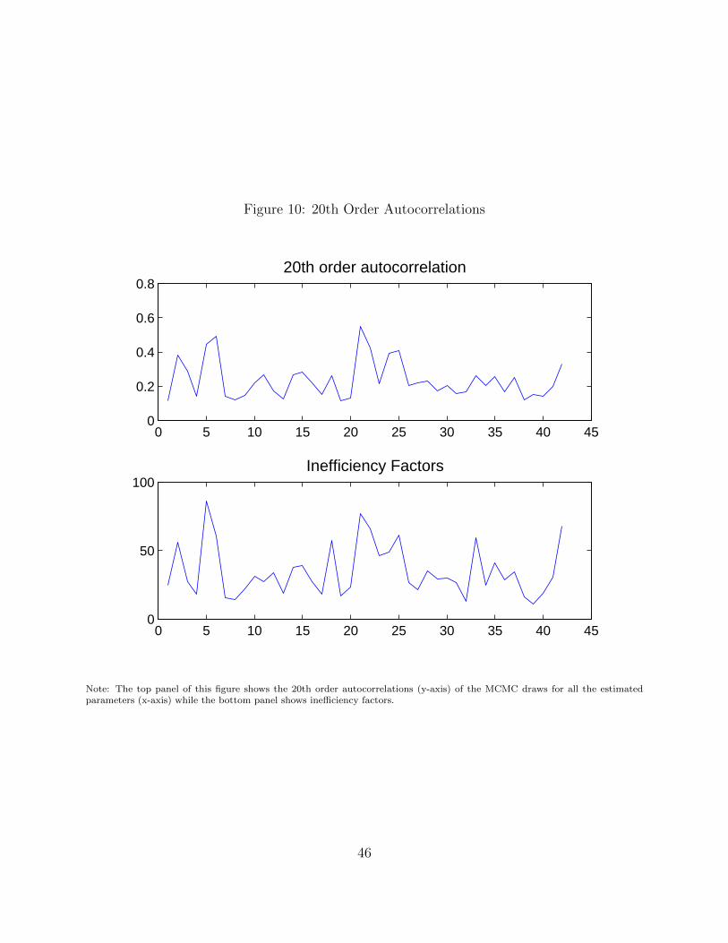
Figure 10: 20th Order Autocorrelations

0 5 10 15 20 25 30 35 40 450

0.2

0.4

0.6

0.820th order autocorrelation

0 5 10 15 20 25 30 35 40 450

50

100Inefficiency Factors

Note: The top panel of this figure shows the 20th order autocorrelations (y-axis) of the MCMC draws for all the estimatedparameters (x-axis) while the bottom panel shows inefficiency factors.

46