how dangerous are drinking drivers?

1198

[Journal of Political Economy, 2001, vol. 109, no. 6]� 2001 by The University of Chicago. All rights reserved. 0022-3808/2001/10906-0005$02.50

How Dangerous Are Drinking Drivers?

Steven D. LevittUniversity of Chicago and American Bar Foundation

Jack PorterHarvard University

We present a methodology for measuring the risks posed by drinkingdrivers that relies solely on readily available data on fatal crashes. Thekey to our identification strategy is a hidden richness inherent in two-car crashes. Drivers with alcohol in their blood are seven times morelikely to cause a fatal crash; legally drunk drivers pose a risk 13 timesgreater than sober drivers. The externality per mile driven by a drunkdriver is at least 30 cents. At current enforcement rates the punishmentper arrest for drunk driving that internalizes this externality wouldbe equivalent to a fine of $8,000.

I. Introduction

Motor vehicle crashes claim over 40,000 lives a year in the United States,approximately the same number of Americans killed over the course ofeither the Korean or Vietnam wars. The death toll in motor vehicleaccidents roughly equals the combined number of suicides and homi-cides, and motor vehicle deaths are 30 times as frequent as accidentaldeaths due to firearms. Motor vehicle accidents are the leading causeof death for Americans aged 6–27.

We would like to thank Joe Altonji, Gary Chamberlain, Austan Goolsbee, Lars Hansen,James Heckman, Guido Imbens, James Poterba, Kenneth Wolpin, two anonymous referees,the editor Robert Topel, and numerous seminar participants for helpful comments andadvice, as well as Christopher Ruhm for generously providing us with data. Financialsupport of the National Science Foundation is gratefully acknowledged.

drinking drivers 1199

Alcohol is often implicated in automobile deaths. According to policereports, at least one driver has been drinking (although not necessarilyover the legal blood-alcohol limit) in over 30 percent of fatal crashes.During the time periods in which alcohol usage is greatest, that pro-portion rises to almost 60 percent.1

Without knowing the fraction of drivers on the road who have beendrinking, however, one cannot possibly draw conclusions about the rel-ative fatal crash risk of drinking versus sober drivers, the externalityassociated with drinking and driving, or the appropriate public policyresponse. For instance, if 30 percent of the drivers had been drinking,over half of all two-vehicle crashes would be expected to involve at leastone drinking driver, even if drinking drivers were no more dangerousthan sober drivers.

Past research has attempted to measure this fraction through the useof random roadblocks and driver stops (Lehman, Wolfe, and Kay 1975;Lund and Wolfe 1991; Hurst, Harte, and Frith 1994).2 While these stud-ies are extremely valuable, they suffer from a number of importantlimitations. First, they are costly to undertake and consequently areperformed only rarely. Second, in such experiments, drivers who havebeen stopped cannot be compelled to submit to alcohol tests. In prac-tice, roughly 10 percent of drivers refuse to participate—presumablythose most likely to have been drinking (Lund and Wolfe 1991). Theassumptions adopted for dealing with this sample selection are criticalto the interpretation of the data. Third, even if the estimates obtainedare reliable, they reflect the specific circumstances at a particular timeand place, and the extent to which the conclusions are broadly gener-alizable is unknown.

In this paper, we adopt a radically different strategy for estimatingthe fraction of drinking drivers and the extent to which their likelihoodof a fatal crash is elevated. Specifically, we rely exclusively on data fromfatal crashes. A priori, it would seem that such an exercise, even iffeasible, would require an extremely restrictive set of assumptions andthe imposition of an arbitrary functional form. Separately identifyingthe fraction of drinking drivers on the road and their relative risk of afatal crash using only the fraction of drinking drivers in fatal crashes isostensibly equivalent, for instance, to determining the relative free-throw

1 Because many fatal crashes involve more than one vehicle, the actual fraction of drink-ing drivers involved in these crashes is lower than the values cited above. Overall, roughly30 percent of drivers in fatal crashes have been drinking, with that percentage rising to50 percent during peak times of alcohol usage.

2 There are also survey data asking drivers whether they have driven when they have“had too much to drink” (Liu et al. 1997). In addition to any question about the accuracyof the responses given, these surveys have not attempted to ask drivers to report thepercentage of miles driven with and without the influence of alcohol. Without that number,accurate estimates of the elevated risk of drinking drivers cannot be computed.

1200 journal of political economy

shooting ability of two basketball players on the basis of only the numberof free throws successfully completed by each. Without knowledge ofhow many free-throw attempts each player had, such an exercise wouldappear futile. In the realm of economics, our task is equivalent to sep-arately identifying per capita income and population on the basis ofonly aggregate income data. Despite the apparent difficulty of this ex-ercise, the assumptions required for identification of the model are inactuality quite natural and do not even require the imposition of ar-bitrary distributional assumptions.

The ability to identify the parameters arises from a hidden richnessin the data due to the fact that crashes often involve multiple drivers.For two-car crashes, the relative frequency of accidents involving twodrinking drivers, two sober drivers, or one of each provides extremelyuseful information. Indeed, given the set of assumptions outlined inSection II, this information alone is sufficient to separately identify boththe relative likelihood of causing a fatal crash on the part of drinkingand sober drivers and the fraction of drivers on the road who have beendrinking. The intuition underlying the identification of the model isquite simple. The number of two-car fatal crash opportunities is dictatedby the binomial distribution. Consequently, the number of fatal two-carcrash opportunities involving two drinking (sober) drivers is propor-tional to the square of the number of drinking (sober) drivers on theroad. The number of fatal crash opportunities involving exactly onedrinking and one sober driver is linearly related to the number of bothdrinking and sober drivers. Identification of the model arises from theseintrinsic nonlinearities. These nonlinearities are not artificially imposedon the problem via arbitrary functional form assumptions, but ratherare the immediate implication of the binomial distribution, which reliesonly on the assumptions to be stated in Section II concerning inde-pendence of crashes and equal mixing of the different types on theroad.

Applying the model to data on fatal accidents in the United Statesover the period 1983–93, we obtain a number of interesting results.Drivers identified by police as having been drinking (but not necessarilylegally drunk) are at least seven times more likely to cause a fatal crashthan drivers with no reported alcohol involvement. Drivers above theblood-alcohol limit of 0.10 are at least 13 times more likely to be thecause of fatal crashes. When we apply the model to other observabletraits, males, young drivers, and those with bad previous driving recordsare also more likely to cause crashes. Drinking, however, is far moreimportant than these other characteristics, and much of the apparentimpact of gender and past driving record actually reflects differentialpropensities to drink and drive across groups. The exception is youngdrivers: sober, young drivers are almost three times as likely to cause a


fatal crash as other sober drivers. The peak hours for drinking anddriving are between 1:00 a.m. and 3:00 a.m., when as many as 25 percentof drivers are estimated to have been drinking. The proportion of drink-ing drivers appears to have fallen by about one-quarter over the courseof our sample. The relative fatal crash risk of drinking drivers, in con-trast, appears to have been stable.

The great majority of alcohol-related driving fatalities occur to thedrinking drivers themselves and their passengers. Since these individualsare likely to have willingly accepted the risks associated with their actions,the role for public policy in preventing these deaths is unclear. Ac-cording to our estimates, roughly 3,000 other people are killed eachyear by drinking drivers. When standard valuations of a life are used,the externality due to drinking drivers’ killing innocent people is 15cents per mile driven. For legally drunk drivers, we estimate the exter-nality at 30 cents per mile driven. At current arrest rates for drunkdriving, the Pigouvian tax that internalizes that externality is $8,000 perarrest.

We also use our estimates of the fraction of drivers who are drinkingand the risk that they pose to analyze the impact of various publicpolicies. A separate literature examines the impact of public policies onfatal car crashes (Cook and Tauchen 1982; Asch and Levy 1987; Safferand Grossman 1987; Homel 1990; Chaloupka, Saffer, and Grossman1993; Grossman et al. 1993; Ruhm 1996). In contrast to previousreduced-form approaches to measuring the impact of alcohol policies,we are able to differentiate between very different underlying behavioralresponses. For instance, we find some evidence that higher beer taxesand stiff punishments for first-time offenders reduce the number ofdrinking drivers, but no evidence that such policies affect the level ofcare that drinking drivers exhibit on the roads. On the other hand,harsh penalties for third-time offenders and large numbers of policeon the road have little impact on the number of drinking drivers, butdrinkers who do drive tend to pose a lower risk. This latter result mayoccur either because a few chronic drunk drivers are deterred or becausethe drunks who do drive are more cautious on the roads.

The remainder of the paper is structured as follows. Section II derivesthe basic model and discusses the sensitivity of the results to alternativemodeling assumptions. Section III describes and summarizes the dataused. Section IV presents the empirical estimates of the relative crashrisk and the number of drinking and sober drivers, as well as a numberof extensions to the basic model. Section V computes the externalityassociated with drunk driving and analyzes the relationship betweenpublic policies, the number of drinking drivers, and the risks that theypose. Section VI presents conclusions.


II. A Model of Fatal Crashes

In this section, we present a simple model of fatal accidents, demon-strating how identification of the underlying structural parameters (thefraction of drivers on the road who have been drinking and the relativelikelihood of causing a fatal crash by drinking and sober drivers) nat-urally emerges from the model. A number of features of the model areworth noting. First, identification relies only on the distribution ofcrashes in a particular geographic area over a given period of time.Consequently, the model does not necessitate comparisons across timesand places that may differ in systematic yet unobservable ways, leadingto biased estimates. Second, although the model is identified off non-linearities, the structural equations that will be estimated follow directlyfrom the restrictions dictated by nature in the form of the binomialdistribution. Third, the approach we outline provides a previously un-attainable flexibility in measuring drinking and driving. The solutionto the model depends only on tallies of fatal crashes, data that are alreadycollected and widely available. Thus parameter estimates can be ob-tained almost without cost for any geographic area or time period ofinterest to the researcher, for example, the Chicago metropolitan area,on weekends between 10:00 p.m. and 2:00 a.m. (although standard errorsincrease as the number of fatal crashes on which the estimate is basedshrinks).

Assumptions of the Model

We begin by outlining the five assumptions underlying the model. Thefirst assumption is as follows.

Assumption 1. There are two driver types, D and S.The terms D and S correspond to drinking and sober drivers, re-

spectively, although other categories of driver types could also be used.Restricting the analysis to two types is done primarily to ease expositionof the model, which readily generalizes to multiple types. In some ofour empirical estimation we allow four types. In theory, any number oftypes could be incorporated if enough data existed. As we demonstratelater, the parameter estimates from a model assuming exactly two typeshave a straightforward interpretation when there is heterogeneity indriver risk within these two categories of drivers.

The second assumption of the model pertains to “equal mixing” ofdrinking and sober drivers on the roads. By equal mixing, we mean twothings: (1) the number of interactions that a driver has with other carsis independent of the driver’s type, and (2) a driver’s type does notaffect the composition of the driver types with which he or she interacts.The term “interaction” is used here to mean a two-car fatal crash op-


portunity in which two cars are close enough that a mistake by one ofthe drivers could cause a fatal accident.3 A formal statement of thissecond assumption requires some notation. Let the total number ofdrivers be Ntotal, and let the total number of drivers of type i be Ni. Byassumption 1, there are only two types, Define I to beN � N p N .D S total

an indicator variable equal to one if two cars interact and equal to zerootherwise. Two drivers are denoted as having types i and j.

Assumption 2. (i) (ii)Pr (iFI p 1) p N /(N � N ). Pr (i, jFI p 1) pi D S

Pr (iFI p 1) Pr ( jFI p 1).Assumption 2 is essentially a homogeneity requirement. Over a small

enough geographic range and time period, assumption 2 is certainlyreasonable. For example, on a particular stretch of highway over a 15-minute period, there may be little reason to think that drinking andsober drivers are not equally mixed. As the unit of observation expandswith respect to either space or time, this homogeneity condition clearlybecomes suspect. We devote a great deal of attention to possible vio-lations of assumption 2 and their impact on the results in the empiricalsection of the paper.

The third assumption of the model is as follows.Assumption 3. A fatal car crash results from a single driver’s error.Assumption 3 rules out the possibility that each of the drivers shares

some of the blame for a crash. As discussed later in this section, whileassumption 3 is critical to the identification of the model, it is possibleto sign the direction of bias introduced by assumption 3 if, in fact, bothdrivers contribute to fatal crashes.

The fourth modeling assumption is as follows.Assumption 4. The composition of driver types in one fatal crash is

independent of the composition of driver types in other fatal crashes.This assumption allows us to move from individual crash probabilities

to probabilities involving multiple crashes. Given the level of aggregationused in the empirical analysis (e.g., weekend nights between the hoursof midnight and 1:00 a.m. in a given state and year), there is little reasonthat this assumption should fail, although for very localized observations(a short stretch of road over a 15-minute time period), it may be lessapplicable.

The final assumption required to solve the model is that drinking(weakly) increases the likelihood that a driver makes an error resultingin a fatal two-car crash. Denote the probability that a driver of type imakes a mistake that causes a fatal two-car crash as vi.

3 Of course, there are different degrees of interactions between vehicles. Two vehiclescan meet at an intersection, pass each other on a two-lane highway, or pass one anotheron a residential street. We abstract from this complexity in our model, but one couldimagine treating the degree of interaction between vehicles as a continuous rather thana discrete variable.


Assumption 5. v ≥ v .D S

The existing evidence concerning the relative crash risk of drinkingand sober drivers overwhelmingly supports this assumption (e.g., Lin-noila and Mattila 1973; Borkenstein et al. 1974; Dunbar, Penttila, andPikkarainen 1987; Zador 1991).

Fatal Crash Data and the Parameters of Interest

Having laid out the assumptions of the model, we derive the link be-tween fatal crash data and the parameters of interest in three steps.First, we derive the formulas corresponding to the likelihood that twocars will interact with one another. Second, we determine the likelihoodof a crash conditional on both the drivers’ types and an interaction thattakes place between two cars. We then back out the probability that agiven pair of driver types will be involved conditional on the occurrenceof a fatal crash. Third, we derive the likelihood function and discussthe identification issues involved in its estimation.

Assumption 2 gives the joint distribution for a pair of driver types,conditional on an interaction between two drivers:

N Ni jPr (i, jFI p 1) p , (1)2(N � N )D S

where i and j are drivers of a particular type, that is, either drinking orsober. So, for example, given that an interaction occurs between twocars, the probability that both are sober drivers is In-2 2(N )/(N � N ) .S D S

teractions between drivers in this model, as reflected in equation (1),are logically equivalent to randomly drawing balls labeled either S or Dout of an urn.

Define A to be an indicator variable equal to one if there is a fatalaccident and equal to zero otherwise. Assumption 3 implies that theconditional probability of a fatal two-car crash given that two drivers oftypes i and j pass on the road is

Pr (A p 1FI p 1, i, j) p v � v � v v ≈ v � v . (2)i j i j i j

The likelihood of a fatal crash is the sum of the probabilities that eitherdriver makes a fatal error minus the probability that both drivers makea mistake. Given that the chance that either driver makes a fatal mistakeis extremely small, the chance that both drivers make an error is vanish-ingly small and can be ignored.4 So, for example, given that two sober

4 There are roughly 13,000 fatal two-car crashes in the United States annually. The totalnumber of vehicle miles driven is approximately 2 trillion. If every car interacted with anaverage of five other cars per mile, then the implied vi is on the order of 10 �9 and theinteraction term is on the order of 10 �18.


drivers interact, the probability of a fatal accident is 2vS. More generally,we could allow for heterogeneity in driver risk within each driver type,as discussed in the extensions to the basic model. In that case, vi andvj in equation (2) represent the mean driver risks for the population ofdrivers of types i and j on the road.

When equations (1) and (2) are multiplied, the joint probability ofdriver types and a fatal crash conditional on an interaction between twodrivers is

N N (v � v)i j i jPr (i, j, A p 1FI p 1) p . (3)2(N � N )D S

In words, given that two random drivers interact, the probability that afatal crash occurs and that the drivers involved are of the specified typesis simply equal to the likelihood that two drivers passing on the roadare of the specified types multiplied by the probability that a fatal crashoccurs when these drivers interact.

The key relationship that we seek is the probability of driver typesconditional on the occurrence of a fatal accident rather than on aninteraction. That value can be obtained from equation (3):

Pr (i, j, A p 1FI p 1)Pr (i, jFA p 1) p

Pr (A p 1FI p 1)

N N (v � v)i j i jp . (4)2 22[v (N ) � (v � v )N N � v (N ) ]D D D S D S S S

Although the expression in equation (4) looks somewhat complicated,it is in fact quite straightforward. For each combination of driver types,the numerator is proportional to the number of fatal crashes involvingthose two types. The denominator is a scaling factor assuring that theprobabilities sum to one.

Let Pij represent the probability that the drivers are of types i and jgiven that a fatal crash occurs. We can explicitly state the values of Pij

by simply substituting for i and j in equation (4):

P p Pr (i p D, j p DFA p 1)DD

2v (N )D Dp , (5)2 2v (N ) � (v � v )N N � v (N )D D D S D S S S

P p Pr (i p D, j p SFA p 1) � Pr (i p S, j p DFA p 1)DS

(v � v )N ND S D Sp , (6)2 2v (N ) � (v � v )N N � v (N )D D D S D S S S


and

P p Pr (i p S, j p SFA p 1)SS

2v (N )S Sp . (7)2 2v (N ) � (v � v )N N � v (N )D D D S D S S S

Note that the ordering of the driver types does not matter. Consequently,in equation (6), the probability of a mixed drinking-sober crash is thesum of the probability that i is sober and j is drinking plus the probabilitythat j is sober and i is drinking.

Examination of equations (5)–(7) reveals that there are only threeequations but four unknown parameters (vD, vS, ND, and NS). Conse-quently, all four parameters cannot be separately identified. Closer ex-amination of equations (5)–(7) reveals that only the ratios of the pa-rameters could possibly be identified. Therefore, let andv p v /vD S

The term v is the relative likelihood that a drinking driverN p N /N .D S

will cause a fatal two-car crash compared to a sober driver, and N is theratio of sober to drinking drivers on the road at a particular place andtime.5 Expressing equations (5)–(7) in terms of v and N yields

2vNP (v, NFA) p , (8)DD 2vN � (v � 1)N � 1

(v � 1)NP (v, NFA) p , (9)DS 2vN � (v � 1)N � 1

and

1P (v, NFA) p . (10)SS 2vN � (v � 1)N � 1

The final step is deriving the likelihood function. The values in equa-tions (8)–(10) provide the likelihoods of observing the various com-binations of driver types conditional on the occurrence of a crash. Fromassumption 4, which provides independence across fatal crashes, andgiven the total number of fatal crashes, the joint distribution of drivertypes involved in fatal accidents is given by the multinomial distribution.Define Aij as the number of fatal crashes involving one driver of type iand one driver of type j and Atotal as the total number of fatal crashes.Then

5 Since we have three observable pieces of data (the number of drinking-drinking,drinking-sober, and sober-sober crashes), one might expect that we might be able to dobetter than to identify only two parameters, the ratios v and N. In fact, although thereare three equations, the three equations are linearly dependent (i.e., the equations sumto one), so in practice only two parameters can be identified.


Pr (A , A , A FA ) pDD DS SS total

(A � A � A )!DD DS SS A A ADD DS SS(P ) (P ) (P ) . (11)DD DS SSA !A !A !DD DS SS

Substituting the solutions to PDD, PDS, and PSS into equation (11) yieldsthe likelihood function for the model. In the empirical work that follows,we perform maximum likelihood estimation of equations (8)–(11), di-rectly linking our empirical estimation strategy to the model. Note thatmaximization of equation (11) with respect to PDD, PDS, and PSS yieldsthe following intuitive result:

A A ADD DS SSˆ ˆ ˆP p , P p , P p . (12)DD DS SSA A Atotal total total

In other words, the maximum likelihood estimate of the fraction ofcrashes involving two drinking drivers is simply the observed fractionof such crashes in the data.

In order to solve the model for v, we take the following ratio, in whichN, the ratio of drinking to sober drivers, cancels out:

2 2 2 2ˆ(A ) (P ) (v � 1) N 1DS DSp p p 2 � v � . (13)2ˆ ˆA A P P vN vDD SS DD SS

It is worth pausing here to note the significance of equation (13), whichsays that it is possible to determine the relative crash risk of drinkingand sober drivers (v) solely on the basis of the observed distribution offatal crashes. The key to this result is the cancellation of the N term.The N disappears from equation (13) because, by the binomial distri-bution, the squared number of interactions between drinking and soberdrivers is in fixed proportion to the product of drinking-drinking andsober-sober interactions. Therefore, information on the relative numberof drinking and sober drivers on the road is not needed to identify themodel.

Defining the value in the left-hand side of equation (13) as R,

2(A )DSR { , (14)

A ADD SS

then rearranging equation (13) and multiplying through both sides byv yields an equation that is quadratic in v:

2v � (2 � R)v � 1 p 0, (15)

the solutions to which are

1208 journal of political economy2�(R � 2) � R � 4R

v p . (16)2

Ignore for the time being values of which do not yield a real-R ! 4,valued solution for v. When the only solution is a limitingR p 4, v p 1,case in which drinking drivers pose no greater risk of causing two-carcrashes than sober drivers. Note that for the distribution of fatalR p 4,crashes precisely matches the distribution of crash opportunities as givenby the binomial distribution. This occurs only when the crash likelihoodsare equal. For all there are two real solutions: one with andR 1 4, v 1 1the other with By assumption 5, which requires drinking driversv ! 1.to be at least as dangerous as sober drivers, we select the first of thosetwo solutions. When a solution for v is obtained, it is straightforward toback out the relative number of drinking and sober drivers. Standarderrors for both v and N are readily attainable from the Hessian of thelikelihood function.6

Now consider the case in which A non-real-valued solution toR ! 4.equation (16) emerges. Values of are not consistent with the bi-R ! 4nomial distribution; that is, there is no combination of v and N thatcan generate this outcome. From equation (14), low values of R resultwhen there are too few drinking-sober crashes. Such values of R mayarise in practice either because of small numbers of observed crashesor because of a violation of the equal mixing assumption, as will bediscussed below. It is important to note, however, that observed valuesof do not invalidate the maximum likelihood estimation. WhenR ! 4

the maximum likelihood estimate of v is one and the maximumR ! 4,likelihood estimate of N is the observed ratio of sober and drinkingdrivers involved in two-car crashes. Note that regardless of the value ofR, standard errors for both v and N can be computed.

Figure 1 provides a sense of how the estimates of v and N vary withthe distribution of two-car crashes. The y-axis in figure 1 reflects v, therelative crash likelihood of drinking drivers. The x-axis is the numberof mixed drinking-sober crashes (ADS). The two curves plotted in the

6 In particular, the first-order condition from maximum likelihood estimation of eq.(11) provides a solution for N in terms of v:

v 1vN p A � A A � A .ZDS DD DS SS( ) ( )[ ] [ ]1 � v 1 � v

From the definitions of N and v, the left-hand side of this equation is ThisN v /N v .D D S S

ratio is the number of two-car crashes caused by drinking drivers relative to the numbercaused by sober drivers. The right-hand side of the equation above expresses that ratiosolely in terms of v and the observed distribution of crashes. Drinking drivers cause

of the crashes between drinking and sober drivers and all crashes involving twov/(1 � v)drinking drivers; sober drivers cause of the crashes between drinking and sober1/(1 � v)drivers and all crashes involving two sober drivers.


Fig. 1.—Estimated relative risk of drinking drivers as a function of observed crash mix.Solid line: ADDp20, ASSp80; dotted line: ADDp50, ASSp50.

figure correspond to alternative numbers of drinking-drinking andsober-sober crashes. The top line is the case in which ADD and ASS (thenumber of fatal crashes involving two drinking and two sober drivers)are 20 and 80, respectively. In the bottom line, both ADD and ASS areheld constant at 50. When the number of drinking-drinking and sober-sober crashes is held constant, the estimated v increases roughly inproportion to the square of the number of crashes involving one soberand one drinking driver, although over the relevant range the relation-ship appears almost linear since the constant of proportionality

is so small. The flat portions of the curves correspond to(1/A A )DD SS

values of described in the preceding paragraph. While the shapesR ! 4of the curves are similar, note that for a given number of mixed drinking-sober crashes, the implied v is much higher when the number of drink-ing-drinking crashes is lower. The intuition for this result is that whendrinking-sober crashes are held constant, a low number of drinking-drinking crashes implies fewer drinking drivers on the road since thenumber of drinking-drinking crashes is a function of the square of thenumber of drinking drivers. In order for a small number of drinkingdrivers to crash into sober drivers so frequently, the drinking driversmust have a high risk of causing a crash.


Incorporating One-Car Crashes

The model above is derived without reference to one-car crashes. In-tuition might suggest that there would be useful information providedby such crashes. In fact, that intuition turns out to be correct only to alimited degree. Since one-car crashes lack the interactive nature of two-car crashes, which provides identification of the model, there is relativelylittle to be gained by adding one-car crashes to the model.

Let lD and lS denote the probabilities that drinking and sober driversmake an error resulting in a fatal one-car crash, paralleling the vD andvS terms in the two-car case. Let C be an indicator for the presence ofa one-car crash; that is, if a one-car crash occurs and equals zeroC p 1otherwise. Let and denote the respective probabilities that aQ QD S

drinking or sober driver is involved in a given one-car crash. Then

l ND DQ p Pr (i p DFC p 1) p (17)D

l N � l ND D S S

and

l NS SQ p Pr (i p SFC p 1) p . (18)S

l N � l ND D S S

Defining we can rewrite the ratio of equations (17) andl p l /l ,D S

(18) as

Q Dp lN. (19)

Q S

Thus, in contrast to the two-car case, it is impossible to separately identifythe parameters of the model using only one-car crashes. Algebraically,adding equation (19) to the two-car crash model provides one additionalequation and one extra unknown. Since N is identified from two-carcrashes, it is possible nonetheless to back out estimates of l. Note,however, that it is the identification coming from the two-car crashesthat is critical to obtaining that parameter, and adding the one-carcrashes does not affect the solution to the two-car case.7

Relaxing the Assumptions

Before we proceed to the data, it is worth considering the way in whicheach of the assumptions made influences the solution to the model,

7 In the empirical estimation, we include one-car crashes for two reasons. First, we areinterested in estimating l, even if identification hinges on two-car crashes. Second, in ourempirical estimates, we shall generally impose equality restrictions across v for differentgeographic areas or time periods. Once such restrictions are imposed, one-car crashesare useful in estimating the parameters of the model.


possible alternative assumptions, as well as the likely direction of biasin the estimation induced by violation of the assumptions.

The assumption of exactly two types is relatively innocuous. The in-troduction of more types allows for greater differentiation of estimatesfor particular subgroups of the population (e.g., drinking teenagers orsober motorists with clean driving records). From a practical perspective,however, the number of two-car crashes is not great enough to supportmore than a small number of categories. In the presence of hetero-geneity within categories (i.e., there is a distribution of driving abilitiesamong drinking and sober drivers), the estimates obtained from thetwo-type model are nonetheless readily interpretable. The estimates ob-tained are weighted averages across drivers in the category, with weightsdetermined by the number of drivers of each ability on the road.8 Thisis a surprising and useful result. Given that we observe drivers only infatal crashes, intuition might suggest that the weights would be basedon the distribution of abilities among crashers rather than drivers as awhole. If our coefficients reflected only the abilities of those in crashes,then the results would be much less useful for public policy since thedistribution of crashers is likely to be very different from the underlyingdistribution of drivers.9

The second assumption, equal mixing/homogeneity on the road, ismuch more critical to the results. This assumption will likely be violatedthrough spatial or temporal clumping of similar types of drivers. Forinstance, if the unit of observation were all crashes in the United Statesin a given year, then it is clear that drinking drivers would not be ran-domly distributed, but rather concentrated during nighttime hours andespecially weekend nights. Even within a smaller unit of analysis (e.g.,weekends between midnight and 1:00 a.m. in a particular state and year)there may be clumping. Roads near bars may contain a higher fractionof drinking drivers, or the proportion of drinking drivers may rise

8 Suppose that driver types D and S have distributions of driver risk given by andf (v)D

Then the probability of a fatal accident given only the types i and j of two interactingf (v).S

drivers is

Pr (A p 1Fi, j, I p 1) p (v � v � v v )f (v , v )dv dv� i j i j i,j i j i j

p E(v ) � E(v ) � E(v v ) ≈ E(v ) � E(v ).i j i j i j

Thus with heterogeneity we can simply reinterpret v as the mean driver risk for the giventypes.

9 In the presence of heterogeneity, our simple model can do no better than to identifythe ratio of the means of the distributions. Identification of higher moments of thedistributions would require imposing arbitrary parametric assumptions.


sharply immediately following bar closings.10 Such a nonrandom distri-bution of drivers will result in a greater number of drinking-drinkingand sober-sober interactions than predicted by the binomial distribu-tion, with correspondingly fewer drinking-sober interactions. Fromequation (14), nonrandom mixing will lead to smaller values of R andconsequently a downwardly biased estimate of v, which is an increasingfunction of R. Conversely, N, the ratio of drinking to sober drivers, willbe biased upward. Violations of this assumption are likely to be lessextreme as the geographic and temporal units of analysis shrink. In fact,that is precisely the pattern revealed by the empirical estimates in Sec-tion IV.

The third assumption requires that one driver be wholly at fault in afatal crash, rather than that both drivers share some fraction of theblame. A simple alternative model would allow both drivers to play arole in the crash: if one driver makes a fatal error, the second driverhas an opportunity to take an action to avoid the crash. Let m denotethe relative inability of drinking drivers to avoid a fatal crash that anotherdriver initiates, with It is straightforward to demonstrate that thism ≥ 1.more general model yields a solution parallelingR p 2 � (v/m) � (m/v),equation (13), but with replacing v. In our basic model, m is implicitlyv/mset equal to one because there is no scope for crash avoidance. If inactuality drinking drivers are less proficient in avoiding crashes initiatedby the other driver, then the parameter identified in our model is ac-tually Allowing for sober drivers to be more skilled in avertingv/m ! v.potential fatal crashes yields a larger estimated value of v for any ob-served distribution of crashes, implying that the estimates for v obtainedin this paper are lower bounds on the true value of how dangerousdrinking drivers are.11

10 It is at least theoretically possible that this assumption could be violated in the oppositeway; i.e., drinking drivers would be less likely to interact with other drinking drivers. Forinstance, if all drinking drivers are traveling north on a two-lane highway and all soberdrivers are traveling south, then drinking and sober drivers will disproportionately interactwith the opposite type.

11 An even more general model would also allow the seriousness of mistakes made bydrivers to vary by type. Let capture the additional difficulty of avoiding a mistaked 1 1made by a drinking driver. The parameters that we identify in two-car and one-car crashesin this expanded model are, respectively, and The term is the seriousness-vd/m l/m. vdweighted ratio of drinking to sober driver mistakes—precisely what we are attempting tocapture in the model; thus this further generalization does not pose any problems to ourestimation. It is worth noting that d does not appear in the solution for one-car crashes.If d were large, one would expect to see big differences in the empirical estimates forone-car and two-car crashes. In practice, the two sets of estimates are close, perhapssuggesting that One could also imagine other possible models of fatal crashes. Ford ≈ 1.instance, the probability of a crash (conditional on the occurrence of an interaction)might be modeled as In other words, each driver has to make a mistake in order forv v .i j

a crash to occur. In such a model, the solution to eq. (13) is for all observed crashR p 4distributions (a result strongly rejected by the data), and only the composite parametervN is identified.


The final two assumptions of the model, independence of crashesand the higher risk that drinking drivers pose, are unlikely to imposeany important biases on the empirical estimates. The existing evidenceoverwhelmingly confirms the assumption that drinking drivers havegreater likelihoods of involvement in fatal crashes. Given the unit ofanalysis of the paper, the independence assumption appears quite rea-sonable. Even if this assumption were to fail (i.e., the presence or ab-sence of one crash influences other potential crashes), there is no reasonto expect that violation of this assumption should systematically bias theestimates in one direction. For bias to occur, the presence of one crashhas to differentially affect drinking-sober crashes relative to drinking-drinking or sober-sober crashes.

III. Data on Fatal Crashes

The primary source of data on fatal motor vehicle accidents in theUnited States is the Fatality Analysis Reporting System (FARS) admin-istered by the National Highway Transportation Safety Administration.Local police departments are required by federal law to submit detailedinformation on each automobile crash involving a fatality. Compliancewith this law was uneven until 1983; thus we restrict the analysis of thepaper to the years 1983–93. Because our primary interest is the impactof alcohol on driver risk, we limit our sample to those hours (8:00 p.m.–5:00 a.m.) in which drinking and driving is most common.12 Our sampleincludes over 100,000 one-car crashes and over 40,000 two-car crashes.During these hours, almost 60 percent of drivers involved in fatal crasheshave been drinking, compared to less than 20 percent of drivers at allother times of the day. Crashes involving three or more drivers, whichrepresent less than 6 percent of fatal crashes, are dropped from thesample. All crashes from a handful of state-year pairs with obvious dataproblems are also eliminated.

Among the variables collected in each fatal crash are information onthe time and location of the accident and whether the drivers involvedwere under the influence of alcohol. In extensions to the basic model,we also utilize information on the age, sex, and past driving record ofthose involved in fatal crashes. Therefore, we exclude from the sampleany crash in which one or more of the drivers are missing informationabout the time or location of the accident, police-reported drinkingstatus, age, sex, or past driving record. Combined, these missing datalead to the exclusion of roughly 8 percent of all crashes.

12 Also the lack of drinking-drinking crashes during the daytime period makes estimationdifficult. During daytime hours, there are typically only a total of about 30 two-car crashesa year in the entire United States in which both drivers have been drinking.


Two measures of alcohol involvement are included in FARS. The firstof these is the police officer’s evaluation of whether or not a driver hadbeen drinking. The officer’s assessment may be based on formal breath,blood, or urine test results or other available evidence such as a driver’sbehavior (for those drivers not killed in the crash) or alcohol on thedriver’s breath. The primary advantage of this measure is that it is avail-able for virtually every driver involved in a fatal crash. There are at leasttwo drawbacks of this variable. First, it does not differentiate betweenvarying levels of alcohol involvement. In particular, no distinction ismade between those drivers who are legally drunk and those who havebeen drinking but are below the legal limit. Second, the measure isoften subjective and relies on the discretion of the police at the sceneof the accident.

In spite of these shortcomings, the police officer’s assessment ofwhether or not a driver has been drinking serves as our primary measureof alcohol involvement. As a consequence, the coefficients we obtainwith respect to the elevated risk associated with drinking and drivingare based on the entire population of drinking drivers, not just thesubgroup of legally drunk drivers. As a check on the results obtained,we also examine a second measure of alcohol involvement, which ismeasured blood-alcohol content (BAC). The major problem with thisvariable is the frequent failure to conduct such tests, despite federal lawmandating that all drivers involved in fatal crashes be tested. Evidencesuggests that the likelihood of BAC testing is an increasing function ofactual blood-alcohol levels, suggesting that this measure will be mostflawed for low-BAC motorists. Thus, for the purpose of analysis, wecompare two groups of drivers: (1) those with measured BAC greaterthan 0.10 percent (the legal limit in most states for most of the sampleperiod) and (2) those who test free of alcohol or who are not testedbut whom police describe as not having been drinking. We eliminatethose who test positive for alcohol but are below the 0.10 threshold.Furthermore, because sample selection in the pool of drivers who aretested for BAC is a major concern when this measure is used, we excludeall crashes occurring in states that do not test at least 95 percent ofthose judged to have been drinking by the police in our sample in thatyear (regardless of whether the motorist in question was tested). Thisrequirement excludes more than 80 percent of the fatal crashes in thesample.

The presence of classification error in each of our measures of drink-ing, like the violations of the model’s assumptions in the previous sec-tion, will almost certainly lead to an underestimate of the relative fatalcrash risk of drinking drivers, making our estimates conservative. Thispoint is discussed in detail in the next section.

The time series of fatalities in all motor vehicle crashes rises from an


TABLE 1Summary Statistics for Fatal Crashes in the Sample:One- and Two-Car Crashes between 8:00 p.m. and 5:00

a.m., 1983–93

Variable Mean

Total number of fatal one-car crashes 103,077Total number of fatal two-car crashes 39,470Percentage of all drivers in fatal crashes:

Reported to be drinking by police 53.4Male 82.2Under age 25 44.0Bad previous driving record 37.2Reported to be drinking and male 45.2Reported to be drinking and under age

25 24.6Reported to be drinking and bad previ-

ous driving record 23.5Percentage of fatal one-car crashes with:

One drinking driver 63.0One sober driver 37.0

Percentage of fatal two-car crashes with:Two drinking drivers 14.2One drinking, one sober driver 53.2Two sober drivers 32.6

Percentage of fatal one-car crashes in re-stricted sample with high BAC re-porting with:

One legally drunk driver 55.9One sober driver 44.1

Percentage of fatal two-car crashes in re-stricted sample with high BAC re-porting with:

Two legally drunk drivers 6.2One legally drunk, one sober driver 47.8Two sober drivers 46.0

Note—Means are based on one- and two-car fatal crashes in FARS data for theyears 1983–93 between the hours of 8:00 p.m. and 5:00 a.m. Drinking status isbased on the police classification of drivers as drinking and includes drivers whowere not legally drunk, except in the bottom portion of the table, where thesample is restricted to crashes in state-year pairs in which at least 95 percent ofthe drivers whom police report to have been drinking were given blood-alcoholtests. A bad driving record is defined as two or more minor blemishes (a movingviolation or previous accident) or one or more major blemishes (previous DUIconviction, license suspension, or license revocation) in the last five years. Valuesin the table are based on the same data that are used in estimation.

initial value of 42,589 in 1983 to a peak of just over 47,000 in 1988 andthen declines to roughly 40,000 by 1993. The percentage of deathsoccurring in crashes with at least one drinking driver steadily falls overthe sample from 55.5 percent in the beginning to 43.5 percent in theend.

Table 1 presents means for the data in our sample.13 Slightly more

13 Because the degree of aggregation in our analysis varies from hour#year tohour#year#state#weekend, standard deviations, minimums, and maximums are notparticularly meaningful.


than half of all drivers involved in fatal crashes are reported to bedrinking by police. Drivers in fatal crashes are mostly male (82.2 per-cent), somewhat less than half are under the age of 25, and about one-third qualify as having bad previous driving records under our defini-tion: two or more minor blemishes in the last three years (anycombination of moving violations and reported accidents) or at leastone major blemish (conviction for driving while intoxicated or licensesuspension/revocation). The fraction of drivers who are both male anddrinking (45.2 percent) is higher than would be expected on the basisof the marginal distributions if gender and drinking were uncorrelated(i.e., ). This implies that males involved in fatal.534 # .822 p .439crashes are more likely to have been drinking than females. Youngdrivers and those with bad previous driving records are also more likelyto have been drinking.

In one-car crashes, 63 percent of drivers are classified as drinking bythe police. Of two-car crashes, 14.2 percent involve two drinking drivers,53.2 percent have exactly one drinking driver, and in the remaining32.6 percent of cases, neither driver was drinking. When we restrict oursample to states with good BAC reporting practices, 55.9 percent ofdrivers in one-car fatal crashes have a BAC over 0.10. In two-car crashes,there are two drivers with BACs over the legal limit 6.2 percent of thetime and exactly one driver over the limit in 47.8 percent of the crashes.

IV. Estimation of the Model

Table 2 presents maximum likelihood estimates of equation (11), fo-cusing on how the relative fatal crash risks for drinking drivers in two-car crashes (v) and one-car crashes (l) are affected as we increasinglydisaggregate the data. Each column represents a different specification,with the distinction between columns being the unit of observation overwhich “equal mixing” of drivers is assumed. Column 1 is the most re-strictive, imposing equal mixing of all drivers in all years, locations, andhours of the day. Equal mixing is unlikely to hold at such a high levelof aggregation. This restriction is continually relaxed as one moves fromleft to right in the table. In column 3, for instance, equal mixing isimposed for crashes in each hour-year pair in the sample (e.g., it isassumed that between 2:00 a.m. and 3:00 a.m. in 1991, drinking andsober drivers are equally mixed across all locations in the United States).By column 8, equal mixing is assumed only within a given hour andweekend status (equal to one on Friday or Saturday night and zerootherwise) for a particular state and year.14 Theory predicts that all the

14 Stated more formally, in maximum likelihood estimation of eq. (11) in col. 8, werestrict v and l to each be the same for all observations but allow N to vary by state#year#hour#weekend.

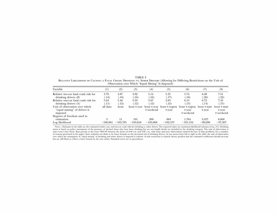
TABLE 2Relative Likelihood of Causing a Fatal Crash: Drinking vs. Sober Drivers (Allowing for Differing Restrictions on the Unit of

Observation over Which “Equal Mixing” Is Imposed)

Variable (1) (2) (3) (4) (5) (6) (7) (8)

Relative two-car fatal crash risk fordrinking drivers (v)

3.79(.14)

4.87(.16)

4.92(.16)

5.14(.16)

5.35(.17)

5.74(.18)

6.48(.20)

7.51(.22)

Relative one-car fatal crash risk fordrinking drivers (l)

5.04(.11)

5.46(.12)

5.50(.12)

5.67(.12)

5.83(.12)

6.13(.13)

6.72(.14)

7.45(.15)

Unit of observation over which“equal mixing” of drivers isimposed

all data hour hour#year hour#year#weekend

hour#region#year

hour#region#year

#weekend

hour#state#year

hour#state#year

#weekendDegrees of freedom used in

estimation 3 11 101 200 884 1,764 3,427 6,668Log likelihood �106,961 �103,795 �103,658 �103,068 �102,537 �101,534 �99,690 �97,307

Note.—Estimates in the table are the estimated relative one- and two-car crash risks for drinking vs. sober drivers. The reported values are maximum likelihood estimates of eq. (11). Drinkingstatus is based on police assessments of the presence of alcohol; those who have been drinking but are not legally drunk are included in the drinking category. The unit of observation isstate#year#day#hour. Data pertain to the years 1983–93 between the hours of 8:00 p.m. and 5:00 a.m., with some state-year observations omitted because of data problems. For a numberof reasons presented in the paper, these estimates are likely to be lower bounds on the increased risk of drinking drivers. As one moves from left to right in the table, the unit of observationover which the assumption of “equal mixing” of drinking and sober drivers is imposed is relaxed. As this restriction is relaxed, theory predicts that the estimated coefficients should increasebut are still likely to reflect a lower bound on the true values. Standard errors are in parentheses.


estimates presented in the table are likely to be lower bounds on thetrue parameters but that the downward bias will be mitigated as onemoves from column 1 to column 8. In fact, that is precisely the patternobserved in the table. The two-car fatal crash risk of drinking driversrises monotonically from four times greater than that of sober driversto over seven times greater.15 For one-car crashes, the value goes fromfive to more than seven times larger. In all cases, the parameters areprecisely estimated, and the null hypothesis of equality between drinkingand sober drivers (i.e., ) is resoundingly rejected. The re-v p 1, l p 1strictions implied by the specifications in columns 1–7 relative to column8 are each rejected with the relevant likelihood ratio test. For this reason,and because theory predicts that less restrictive specifications shouldminimize the downward bias, we take column 8 as our preferred spec-ification.16 All results presented in the remaining tables correspond tocolumn 8.

Although the parameters are not directly comparable to past estimatesin the literature, it is nonetheless useful to consider relative magnitudes.Zylman (1973) finds that the relative crash risk of those with positivelevels of alcohol is only 2.2 times that of sober drivers, much smallerthan our estimates. The reason underlying his estimate of a low impactis that drinking drivers in his sample are disproportionately made upof low-BAC drivers. More informative are the estimates of Borkensteinet al. (1974), who find the relative likelihood of causing a fatal crashto be two times higher for drivers with BACs between 0.05 and 0.099,10.1 times higher for BACs between 0.10 and 0.149, and 30–40 timesgreater for BACs over 0.15. For reasonable distributions of BACs acrossdrinking drivers, the results of table 2 are consistent with the Borken-stein et al. estimates. Zador (1991), using FARS data in conjunction withthe results of the national roadside testing survey of Lund and Wolfe(1991), estimates that BACs of 0.05–0.09 are associated with nine timesgreater risk, BACs of 0.10–0.15 are associated with 50 times greater risk,and BACs above 0.15 have 300–600 times greater risk. These estimatesare far greater than those that we obtain. Zador’s study is subject to thecritiques of roadside surveys discussed earlier in this paper. His high-risk estimates, especially at the highest BAC levels, can be explained by

15 To the extent that the drinking drivers, when they are themselves sober, are syste-matically safer/more dangerous than other sober drivers, this coefficient gives a biasedestimate of the incremental effect of alcohol on driver risk. Previous research (Hurst etal. 1994) suggests that drinking drivers, when sober, are actually safer than the typicalsober driver. If that is the case, then the coefficients in table 2 understate the true impactof alcohol on driver risk. Estimates that further disaggregate drivers by type, presentedbelow, will also shed light on this issue.

16 One could imagine further disaggregating the data. The main stumbling block is lackof data. By col. 8, we are allowing over 6,000 different cells in which there are approximately43,000 two-car crashes.


TABLE 3Estimates of the Relative Crash Risk of Drinking vs. Sober Drivers (Allowing

for Risk to Vary across Years)

Year

Relative Two-CarFatal Crash Risk

for DrinkingDrivers (v)

(1)

Relative One-CarFatal Crash Risk

for DrinkingDrivers (l)

(2)

Implied Fraction ofDrivers That Have Been

Drinking (8:00 p.m.to 5:00 a.m.)

(3)

1983 6.74 6.83 .205(.80) (.56) (.016)

1984 6.34 6.25 .221(.62) (.41) (.013)

1985 8.40 7.54 .185(.78) (.50) (.012)

1986 6.82 7.07 .206(.63) (.45) (.012)

1987 8.29 7.26 .198(.71) (.44) (.011)

1988 7.16 7.57 .188(.66) (.49) (.012)

1989 8.01 7.77 .177(.74) (.51) (.011)

1990 7.69 7.72 .182(.73) (.52) (.012)

1991 8.89 8.60 .161(.88) (.63) (.012)

1992 7.34 8.08 .164(.80) (.64) (.013)

1993 7.59 7.98 .153(.85) (.66) (.014)

F-test: equality ofcoefficientsacross years 6.78 10.93 26.21

Note.—Values are maximum likelihood estimates of eq. (11), allowing the relative crash risks of drinking and soberdrivers to vary by year. The implied fraction of drinking drivers (col. 3) is calculated on the basis of the estimates incols. 1 and 2 and the means of the data in our sample (between the hours of 8:00 p.m. and 5:00 a.m., 1983–93). Adriver does not have to be legally drunk to be categorized as drinking. Note that in the estimation, the fraction ofdrinking drivers is allowed to vary by state#year#weekend#hour. Thus the estimates in this table are comparable tocol. 8 of table 2. Coefficients for each year are estimated separately. For the reasons stated in the paper, the values incols. 1 and 2 are likely to be lower bounds, and the value in col. 3 is likely to be an upper bound. Standard errors arein parentheses. The reported F-test is asymptotically distributed with 10 degrees of freedom. The .05 critical value2xfor this statistic is 18.3.

noting that the highest BAC range is likely to be most underrepresentedin the voluntary roadside survey used. When this underestimate of thefraction of high-BAC drivers on the road is compared to the true in-volvement rate of high-BAC drivers in fatal accidents, the result is sureto overestimate the relative risk at this BAC level.

Table 3 presents separate estimates of relative crash risk across theyears of our sample. For both one-car and two-car crashes, the parameterestimates are fairly stable. A test of the null hypothesis of equality acrossall of the years, reported in the bottom of the table, cannot be rejectedin either case. Given that each year’s estimates are derived indepen-


dently, the stability of the parameters suggests that the estimation ap-proach is robust.

Column 3 of table 3 presents the implied fraction of drivers in thesample who have been drinking.17 To the extent that estimates of therelative risks of drinking drivers are downward biased in columns 1 and2, the fraction of drinking drivers will be biased upward. The estimatesof drinking drivers range from a high of 22.1 percent in 1984 down toa low of 15.3 percent in 1993. There is a discernible downward trendin the fraction of drinking drivers over the period. The null hypothesisof a constant share of drinking drivers across all years is rejected at the.01 level.18

Table 4 breaks down the estimates by hour of the day. Once again,the relative risk for two-car fatal crashes is stable, and equality across allhours cannot be rejected. One-car crash risks vary enough that the testof equality is rejected. The relative risk of drinking drivers appears tobe somewhat lower between 8:00 p.m. and 10:00 p.m., perhaps as a resultof a less lethal composition of drinking drivers on the roads duringthese early hours. The peak hours for drinking and driving are between1:00 a.m. and 3:00 a.m., as reported in column 3. More than one-quarterof drivers appear to have some alcohol in their system during thesehours. This is more than twice as high as before 10:00 p.m. and after4:00 a.m.

Table 5 reports the sensitivity of the basic results on drinking anddriving to the alternative assumptions discussed in Section III as well asto various forms of measurement error. The first row of the table con-tains the baseline estimates for comparison purposes. Each of the re-maining rows reflects a different violation of the assumptions. If crashavoidance matters in two-car crashes (violating assumption 3) and drink-ing drivers are 25 percent less successful in getting out of the way( ), then the estimated impact of alcohol rises above nine inm p 1.25both two-car and one-car crashes and 11 in one-car crashes.19

17 These estimates are derived in two steps. First, v and l are estimated, allowing theratio of sober to drinking drivers to vary by state#year#hour#weekend. Then v and lare fixed at the maximum likelihood estimates from the first step and the optimal N isestimated. Then N is transformed into the percentage of drinking drivers, with the ap-propriate standard errors calculated using the delta method.

18 The estimated fraction of drinking drivers is broadly consistent with numbers obtainedfrom other approaches. In a national roadside survey, Lund and Wolfe (1991) report that8.3 percent of those who provide BACs had alcohol levels greater than 0.05. If all of thosewho refused to provide BACs had been drinking, then the total fraction of drinkers intheir sample could be as high as 16.3 percent.

19 Since the identified parameters are and mN, the risks of drivers in one- andv/m, l/m,two-car crashes are simply scaled up by the relative crash avoidance factor m. Althoughone-car crashes are not directly affected by violations in this assumption, the estimates ofone-car crashes rely on the fraction of drinking drivers on the road, which is identifiedthrough the two-car crashes. As a result, is identified rather than l, paralleling ’sl/m v/midentification rather than v.


TABLE 4Estimates of the Relative Crash Risk of Drinking vs. Sober Drivers (Allowing

for Risk to Vary by Time of Day)

Time of Day

Relative Two-Car FatalCrash Risk

for DrinkingDrivers (v)

(1)

Relative One-CarFatal Crash Risk

for DrinkingDrivers (l)

(2)

Implied Fraction ofDrivers That Have

Been Drinking (8:00 p.m.to 5:00 a.m.)

(3)

8:00 p.m.–9:00p.m.

6.33(.55)

5.55(.36)

.136(.008)

9:00 p.m.–10:00p.m.

6.82(.57)

5.95(.37)

.145(.008)

10:00 p.m.–11:00p.m.

7.16(.58)

7.00(.42)

.157(.009)

11:00 p.m.–midnight

7.60(.59)

7.96(.45)

.180(.009)

Midnight–1:00a.m.

8.36(.66)

8.80(.48)

.209(.009)

1:00 a.m.–2:00a.m.

7.33(.64)

7.68(.42)

.275(.011)

2:00 a.m.–3:00a.m.

6.48(.61)

7.28(.42)

.296(.012)

3:00 a.m.–4:00a.m.

7.28(.90)

8.85(.72)

.222(.016)

4:00 a.m.–5:00a.m.

7.68(1.17)

9.74(1.10)

.137(.019)

F-test: equality ofcoefficientsacross hours 6.62 42.51 236.63

Note.—Values are maximum likelihood estimates of eq. (11), allowing the relative crash risks of drinking and soberdrivers to vary by hours of the day. The implied fraction of drinking drivers (col. 3) is calculated on the basis of theestimates in cols. 1 and 2 and the means of the data in our sample (fatal crashes between the hours of 8:00 p.m. and5:00 a.m., 1983–93). A driver does not have to be legally drunk to be categorized as drinking. Note that in the actualestimation, the fraction of drinking drivers is allowed to vary by state#year#weekend#hour. Thus the estimates inthis table are comparable to col. 8 of table 2. Coefficients for each hour of the day are estimated separately. For thereasons stated in the paper, the values in cols. 1 and 2 are likely to be lower bounds, and the value in col. 3 is likelyto be an upper bound. Standard errors are in parentheses. The reported F-test is asymptotically distributed with2xeight degrees of freedom. The .05 critical value for this statistic is 15.5.

Violations of equal mixing (assumption 2) might likely occur throughan increased probability of same type interactions beyond that given bythe binomial distribution. To consider such violations, we augment theinteraction stage of the model. If is the fraction of drinkingN /ND total

drivers on the road, then in the augmented model the probability thattwo drivers passing are both drinking drivers is rather2(1 � D)(N /N )D total

than ; that is, drinking drivers are D times more likely to2(N /N )D total

interact with one another than would be suggested by the binomialdistribution. Sober drivers are assumed to be precisely enough morelikely to interact with sober drivers to maintain the assumption that theoverall fraction of interactions by driver type reflects the fraction ofdrivers on the road. Given any value of D corresponding to some degreeof unequal mixing, we can estimate this expanded model in order toassess the sensitivity of our estimates to violations of assumption 2. In-

TABLE 5Sensitivity of the Estimates to Violations of the Modeling Assumptions and the Presence of Measurement Error

Relative Two-Car FatalCrash Risk for Drinking

Drivers (v)(1)

Relative One-Car FatalCrash Risk for Drinking

Drivers (l)(2)

Implied Fraction of Drivers WhoHave Been Drinking

(8:00 p.m. to 5:00 a.m.)(3)

Baseline 7.51(.22)

7.45(.15)

.186(.004)

Drinking drivers 25 percent less efficientat avoiding crashes initiated by otherdrivers

9.38(.28)

9.31(.19)

.155(.003)

Drinking drivers 10 percent more likelyto interact with drinking drivers thanwith sober drivers

9.60(.26)

9.00(.18)

.160(.003)

5 percent of drivers misclassified becauseof random measurement error

11.99(.19)

11.71(.05)

.135(.001)

5 percent of drinking drivers misclassifiedas sober

9.73(.14)

9.31(.04)

.177(.001)

In 5 percent of crashes all drivers are re-ported as sober, regardless of truedrinking status

11.23(.34)

10.12(.23)

.166(.004)

Note.—The baseline specification in the first row corresponds to col. 8 of table 2. The other values reported in the table are estimates of the true parameters impliedby the coefficients in the baseline specification if that baseline specification is contaminated in the named manner. Crash avoidance represents a violation of assumption3. Non–equal mixing violates assumption 2. The last three rows of the table report three different types of measurement error.


creased clustering of same-type drivers corresponds to lower predictedvalues of R in the model. To offset this effect and explain the observedR in the data, v must increase (and N decrease). The result in the thirdrow of table 5 shows that a 10 percent increase in drinking-drinkinginteractions would lead to an approximately 25 percent increase in theestimates of one- and two-car relative risks.

An implicit assumption of the model is that driver types are known.In fact, as discussed in Section III, we use the police officers’ assessmentof the drinking status of involved drivers, which is a potentially imperfectmeasure. The remaining rows of table 5 examine the sensitivity of ourestimates to three alternative forms of driver misclassification. Thefourth row of the table corresponds to a case in which 5 percent of theobservations are randomly misrecorded; that is, a drinking driver is aslikely to be mistakenly reported as sober as vice versa. In this case, theestimated risk of drinking drivers will be biased toward zero by approx-imately 40 percent. Our results are sensitive to this type of measurementerror because the few drinking-drinking crashes have the greatest impacton the estimates. Given the rarity of drinking-drinking crashes relativeto drinking-sober crashes, such measurement error will exaggerate thenumber of drinking-drinking crashes; that is, the true number of drink-ing-drinking crashes is even smaller than that observed in the data.Previous research suggests, however, that this type of measurement erroris not the most likely scenario. Lund and Wolfe (1991) present evidencethat police officers systematically report drinking drivers to be sober,but not vice versa. If 5 percent of drinking drivers are misreported inthis manner, then the true v, although still biased, is not as sensitive, asis the case with classical measurement error. A final misclassificationstory assumes that reporting errors are correlated within a particularcrash. Different police officers may have divergent standards for clas-sifying an individual as drinking because of the methods used to de-termine drinking status or the officer’s skill in identifying drinking driv-ers. From equations (13) and (14), it is clear that such systematicmeasurement error will impart a large downward bias on v because anymisclassification of this type will shift crashes from the numerator tothe denominator of R. For instance, if 5 percent of police officers fillingout crash reports always report both drivers sober, even if they are drink-ing, then the true v is almost 35 percent higher than our baselineestimate.

Examining Other Driver Traits

Although the comparisons presented thus far are limited to drinkingversus sober drivers, the model is equally applicable to other compar-isons. Table 6 presents results for a range of other dimensions. The first


TABLE 6Estimating Relative Fatal Crash Risks on the Basis of Other Driver

Characteristics

ComparisonGroups

Relative Two-Car FatalCrash Risk for First

Category Named(1)

Relative One-Car FatalCrash Risk for First

Category Named(2)

Implied Fractionof Drivers in the

First CategoryNamed (8:00 p.m.

to 5:00 a.m.)(3)

All drinking vs.sober

7.51(.22)

7.45(.15)

.186(.004)

Legally drunk vs.sober

13.24(1.17)

14.39(1.05)

.080(.011)

Under age 25 vs.all others

1.39(.18)

1.66(.11)

.353(.009)

Male vs. female 3.38(.21)

1.95(.05)

.719(.005)

Bad driving rec-ord vs. cleandriving record

2.41(.13)

1.85(.06)

.254(.006)

Note.—Values in cols. 1 and 2 are maximum likelihood estimates of the fatal crash risk of the first group namedrelative to the second group named. All specifications assume equal mixing by hour#state#year and therefore arecomparable to col. 8 of table 2. Estimates are based on the same data sample used in table 2, except in the comparisonof legally drunk to sober drivers, where only those state-year pairs that report blood-alcohol levels for 95 percent ofthose drivers identified as drinking by the police are included in the sample. Standard errors are in parentheses.

row of table 6 presents as a baseline the results from drinking and soberdrivers. The second row presents a comparison of drivers with BACsgreater than 0.10 (as opposed to all drinking drivers) relative to soberdrivers. As noted earlier, owing to sample selection concerns, we includeonly accidents in state-year pairs in which a high fraction of drivers aretested. As would be expected, the results for legally drunk drivers areeven stronger than for all drinking drivers. Drivers over the legal BAClimit of 0.10 have a relative risk for fatal crashes that is 13–14 timeshigher than that of sober drivers. This number is almost twice as greatas for all drinkers, including those who are not legally drunk. Approx-imately 8 percent of the drivers on the road during the hours we ex-amine appear to be over the 0.10 limit, where this number is again mostappropriately interpreted as an upper bound. The estimates are rela-tively imprecise because many states have poor records of BAC testing,leading them to be excluded from the sample.

Rows 3–5 consider other categories into which drivers can be divided.Drivers under the age of 25 are 40–70 percent more likely to cause fatalcrashes. The estimate of the fraction of young drivers on the road (35percent) appears reasonable. Grossman et al. (1993) report that thoseunder the age of 25 accounted for 20 percent of drivers in 1984, butyounger drivers are likely to make up a disproportionate fraction ofnighttime drivers. Males are over three times as dangerous as femaledrivers for two-car crashes and are at two times higher risk for one-car


fatal crashes. As will be demonstrated below, however, a large fractionof this gap is due to more frequent drinking and driving among males.Finally, those with bad driving records (either two or more minor blem-ishes on their driving record in the past three years or one or moremajor blemishes) appear to be more than twice as dangerous on theroads. Although table 6 reports significant increases in risk associatedwith other driver characteristics, it should be stressed that alcohol usageis far and away the best predictor of increased crash risk.20

The results presented thus far fail to take into account possible in-teractions between the various risk factors such as drinking status, gen-der, and age. To the extent that risk factors are correlated with oneanother, the results of table 6 may be misleading. Table 7 reports esti-mates that allow for interactions between drinking status and the otherrisk factors. In order to do so, we expand our model to allow for fourdriver types rather than two. All of the intuition from the two-type modelpresented in Section II continues to hold in the n-type case. Panel A oftable 7 allows for differential fatal crash risk for young and old driverswho have or have not been drinking. Sober drivers over the age of 25are the lowest-risk drivers and serve as a baseline. Interestingly, youngsober drivers are almost three times as likely to cause fatal crashes asolder sober drivers, but age has little impact on fatal crash risk amongdrinking drivers. Most likely, this reflects the fact that young drinkingdrivers tend to have low BACs relative to older drinking drivers. Incolumn 3, we estimate that roughly one in four young drivers has beendrinking in our sample, compared to one in six older drivers.

Panel B of table 7 reports the results of interacting drinking statuswith driver gender. Sober female drivers are the safest. Sober male driv-ers are 36 percent more likely to cause fatal two-car crashes and 10percent more likely to cause fatal one-car crashes. Males who have beendrinking are almost nine times more dangerous than sober females andare a 60 percent greater risk than drinking females. The gap betweenmale and female drivers shrinks substantially when drinking status istaken into account.

Panel C of table 7 shows interactions between drinking status andpast driving record. Sober drivers with bad past records are almost twiceas likely to cause two-car fatal crashes as sober drivers with clean records.Interestingly, however, the impact of driving record shrinks substantiallyin percentage terms among those who have been drinking. Those with

20 Consistent with our results, insurance premiums tend to be higher for young drivers,those with bad previous driving records, and male drivers. Auto insurance is highly reg-ulated, however, so it is difficult to know if the magnitude of differences in premiums inan unregulated market would correspond to our estimates. A further complication is thatinsurance premiums take into account not only fatal crashes but also nonfatal accidentsand potential property damage.


TABLE 7Relative Fatal Crash Risk (Allowing for Interactions between Drinking and Other

Driver Characteristics)

Driver Classification

Two-Car FatalCrash Risk Relative

to BaselineCategory

(1)

One-Car FatalCrash Risk Relative

to BaselineCategory

(2)

Implied Fractionof Drivers in the

First CategoryNamed (8:00 p.m.

to 5:00 a.m.)(3)

A. Age

Under 25#drinking 10.88(.57)

10.79(.40)

.083(.003)

Over 25#drinking 10.13(.46)

8.56(.27)

.115(.003)

Under 25#not drinking 2.78(.13)

2.30(.06)

.231(.004)

Over 25#not drinking 1.00 1.00 .572(.004)

B. Gender

Male#drinking 8.57(.94)

6.93(.36)

.169(.005)

Female#drinking 5.18(.77)

4.37(.38)

.044(.004)

Male#sober 1.36(.17)

1.09(.05)

.594(.007)

Female#sober 1.00 1.00 .194(.006)

C. Past Driving Record

Bad drivingrecord#drinking

9.47(.55)

8.11(.35)

.080(.003)

Clean drivingrecord#drinking

7.52(.38)

6.91(.24)

.118(.003)

Bad drivingrecord#sober

1.92(.11)

1.37(.04)

.212(.004)

Clean drivingrecord#sober

1.00 1.00 .590(.004)

Note.—Values in cols. 1 and 2 are maximum likelihood estimates of the fatal crash risk of the named group relativeto the named baseline group (i.e., the group with a relative risk defined to be equal to one). All specifications assumeequal mixing by state#year#day#hour and therefore are comparable to col. 8 of table 2. Estimates are based on thesame data sample used in table 2. Standard errors are in parentheses.

bad driving records who have been drinking are roughly 25 percentmore likely to cause fatal two-car crashes than drinking drivers withgood records.

V. Externalities and Public Policy

In this section we examine the public policy implications of the estimatesobtained above. We focus on two sets of questions: (1) How big is theexternality associated with drinking and driving, and (2) what impact


do current public policies have on both the number of drinking driversand the risk that these drivers pose?

We begin with the question of externalities.21 We make a number ofassumptions in what follows, all of which have the effect of understatingthe true negative externality. First, the analysis here is limited strictly todeaths in fatal crashes. If injuries, property damage, and lost welfaredue to behavioral distortions (e.g., sober drivers being afraid to driveat night for fear of being hit by a drinking driver) were included, theestimates would be substantially higher. Second, we assume that if adrinking driver dies as a result of a crash that he causes, then he bearsthe cost of his actions. Presumably, when choosing to drive after drink-ing, he took the risk into account. Any suffering of friends and familythat the driver does not internalize is left out of the calculation. Third,and perhaps more questionable, we assume that a parallel logic appliesto passengers in the drinking driver’s vehicle; that is, they are willingparticipants and thus have chosen to accept the risk associated withriding with a drinking driver.22 Thus, in the externality calculations thatfollow, we include only the deaths of pedestrians and occupants of ve-hicles who die in crashes caused by a driver in another vehicle who hasbeen drinking. We also present estimates under alternative assumptionsfor comparison purposes.

In 1994, 40,716 people died in motor vehicle crashes in the UnitedStates. Of these, 27,023 were killed in crashes that involved no driversreported by the police to have been drinking.23 Another 8,234 fatalitiesoccurred in one-vehicle crashes in which the driver was drinking. On

21 There are a substantial number of papers that attempt to measure the costs thatalcohol imposes on society (e.g., Rice, Kelman, and Miller 1991; Harwood, Fountain, andLivermore 1998), with the typical estimate roughly $150 billion annually in 1998 dollars.Much of this research fails to distinguish between costs borne by alcohol users and costsborne by society, and all these papers exclude the utility that individuals obtain fromdrinking. Manning et al. (1989) draw the distinction between internalized and externalizedcosts, arguing that the optimal Pigouvian tax on alcohol is much higher than the currenttax level.

22 Passengers who bear increased risk of death because they are riding with drinkingdrivers are worse off. In that sense, drinking drivers do impose an externality on theirpassengers. Given the ability of passengers and drivers to negotiate jointly optimal con-sumption and travel patterns, however, it is not clear that there is a market failure betweendriver and passengers that should be corrected through government intervention. Thisis less likely to be true of children of the drinking drivers. Only 7 percent of passengersdying in vehicles driven by drinking drivers were under the age of 15. To the extent thatdrivers or passengers are systematically misinformed about the risks of drinking and driv-ing, there may be an information dissemination role for public policy. In any specificinstance, passengers are likely to have less precise information about the state of intoxi-cation of the driver and the associated risk, although there is no reason to believe thatpassengers should systematically underestimate this risk.

23 A substantial fraction of pedestrians involved in fatal crashes have been drinking. Theyare not included here.


the basis of the logic of the preceding paragraph, these deaths are alsoexcluded from our externality estimate.

There are a number of different kinds of deaths that qualify as anexternality. In two-vehicle crashes in which both drivers were drinking,583 people died. We categorize half of these deaths (292) as externalitiesunder the assumption that fatalities are evenly split between the vehiclethat caused the crash and the other vehicle. Although the drivers ofboth vehicles were drinking, in our model only one of the drivers makesa fatal error. An additional 2,306 fatalities occurred among passengersof vehicles driven by sober drivers who died in two-vehicle crashes withdrinking drivers. On the basis of our model, or 76.5(v � 1)/(v � 1)percent of these deaths would have been avoided if the driver had notbeen drinking. This translates into an additional 1,764 lives. Extrapo-lating our estimates to crashes with more than two vehicles and applyingthe same set of rules yields 308 more deaths that are classified as ex-ternalities. Finally, 631 pedestrians were killed by drinking drivers. Un-der the assumption that the relative risk of drinking drivers for killingpedestrians mirrors the estimates for one-vehicle crashes, or(l � 1)/l

86.6 percent of these pedestrian deaths are attributable to alcohol. Com-bining all these categories, we estimate a total of 2,910 traffic fatalitiesin 1994 that without question should be classified as externalities as aresult of drinking drivers. If passengers in vehicles driven by drinkingdrivers are also included in this calculation, the number would rise toabout 5,000.

Value of life analyses such as Viscusi (1992) typically assign dollaramounts between $1 million and $5 million per life lost. With a valueof $3 million, the externality associated with lost lives due to drinkingand driving in 1993 was almost $9 billion. This calculation representsa lower bound because our estimates of how dangerous drinking driversare is likely to be biased downward because injuries and property lossare excluded, as are deaths of all passengers in the car of the driver atfault. The Federal Highway Administration (1996) estimates that thereare 2.3 trillion vehicle miles traveled each year. According to Festin(1996), 370 billion of these miles are driven during the hours coveredby our sample, 8:00 p.m. to 5:00 a.m. Our estimates suggest that 15.3percent of drivers in this time period were drinking, which translatesinto 56.6 billion miles driven by drinking drivers.24 This implies a neg-ative externality of 16 cents per mile driven by drinking drivers (in-cluding those who have been drinking but are not legally drunk). If wereplicate the analysis above but instead use our estimates of the risk and

24 The parameter N gives the ratio of interactions by drinking drivers to those by soberdrivers. Under assumption 2, N can be used to compute the fraction of drinking driverson the road. To translate this fraction into miles driven, we are assuming that drinkingand sober drivers have approximately the same number of interactions per mile.


fraction of legally drunk drivers alone (see table 6), the externalityalmost doubles to 30 cents per mile driven.25 This calculation impliesthat almost all the costs of drinking drivers are concentrated amongthose who are legally drunk.

One way to correct this externality is to tax alcohol consumptiondirectly. If the typical drunk driver consumes eight drinks prior to driv-ing and makes a 10-mile trip, then the necessary tax per drink to in-ternalize this externality would be 37.5 cents. An alcohol tax is an ex-tremely blunt instrument, however, because most alcohol consumptionis not followed by motor vehicle operation. Taxing alcohol consumptionto reduce drinking and driving introduces distortions into consumptiondecisions of those who do not drink and drive.

A more direct means of correcting the problem is to enforce drunkdriving laws. In 1994, there were approximately 1.1 million arrests fordriving under the influence (DUI), or roughly one arrest for every27,000 miles driven by drunk drivers. In terms of internalizing the ex-ternality, the appropriate punishment for those arrested for drivingdrunk would be $8,000 per arrest, or the utility equivalent of this inlicense suspensions, increased insurance premiums, lost wages, embar-rassment, or jail time. For most first-time offenders, the likely punish-ment is at or below this level: a small fine, perhaps a 30-day licensesuspension, and perhaps one night in jail. For many third-time offend-ers, however, the punishment can be substantial: a three-year licensesuspension and 30 days in jail would not be uncommon. Thus it appearsthat existing punishments are not radically out of line with what mightbe optimal.

The Impact of Public Policies

We now switch attention to the impact of various state policies on thenumber of drinking drivers and the risks that they pose. A number ofstudies have examined the link between drunk driving laws, alcoholtaxes, and motor vehicle fatalities (e.g., Cook and Tauchen 1982; Aschand Levy 1987; Saffer and Grossman 1987; Homel 1990; Chaloupka etal. 1993; Grossman et al. 1993; Ruhm 1996). Previous research is “re-duced form” in the sense that the estimates obtained capture the totalimpact of policy changes on fatalities but do not shed light on theunderlying behavioral parameters. For instance, if the number ofalcohol-involved motor vehicle fatalities is found to fall when the pun-ishment for repeat DUI offenders increases, existing research would notshed light on whether there were fewer drunk drivers on the roads or

25 The internalized cost of fatal crash deaths per mile driven is about three times largerthan the magnitude of the externality, or almost $1 per mile for legally drunk drivers.


whether drunk drivers choose to drive more carefully after the lawschange. Learning about these behavioral parameters is critical to thedevelopment of optimal public policy (Heckman 2000).

Our estimation approach allows us to begin to shed light on thesebehavioral parameters. Using the estimates of Section IV as dependentvariables, we are able to separately examine the number of drinkingdrivers and their relative risk of causing a fatal crash. We caution, how-ever, that the results presented below represent only a first step in thisdirection.

Our regression specification takes the following form:

′depvar p policy G � X F � h � e , (20)st st st t st

where s indexes states, t reflects years, and depvar is any one of a numberof measures of interest: fraction of drinking drivers on the road, relativetwo-car fatal crash risk (v), and relative one-car fatal crash risk (l). Thesemeasures are constructed in a manner identical to those presented intable 4, except that separate estimates are obtained for each state-yearpair.26 The explanatory variables of primary interest are measures ofstate alcohol policies discussed below. Other control variables are thefraction of the state population between the ages of 15 and 24, between25 and 54, or over age 55; the percentage of state residents in metro-politan areas; percentage black; and state unemployment rates. Yeardummies are also included. In some specifications, state random effectsor region fixed effects corresponding to the nine census regions arealso added.27

Our measures of state alcohol policies are admittedly crude. We in-clude the state beer excise tax per case (measured in 1993 dollars). Weinclude two variables for sentence severity corresponding to first- andthird-time offender punishments. Drunk driving penalties have two pri-mary components: license suspension and jail time. States with bothlicense suspensions of 30 or more days and mandatory jail time areassigned two points for first-offense severity. If only one of the conditionsapplies, one point is given. If neither applies, a zero is assigned. Forthird-time offenders, one point each is given for license suspensions ofthree or more years and mandatory jail sentences of 30 or more days.28

The final state policy variable is the number of police per capita, which

26 In contrast to estimated right-hand-side variables, which lead to errors-in-variables biasand also require standard error corrections (Murphy and Topel 1985), estimated left-hand-side variables do not pose any special econometric problems as long as this estimationerror is uncorrelated with the explanatory variables.

27 Because there is so little within-state variation in alcohol policies over this time period,models with state fixed effects are too imprecisely estimated to be useful.

28 We have experimented with a variety of other approaches to capturing the severityof punishments, all of which yield categorically similar results.


is a (relatively crude) measure of the certainty of punishment for drivingwhile intoxicated.

Table 8 reports the results of the analysis. Each column of the tablepresents results for a different dependent variable. Column 1 is theoverall fraction of drinking drivers in fatal crashes. This measure mirrorsthe reduced-form approach of previous studies. Columns 2–4 show re-sults for our three estimated parameters from the model (v, l, and, N).Panel A of the table is estimated using weighted least squares, withweights based on the number of two-car crashes in the state-year. PanelsB and C of the table are identical to panel A except that state-levelrandom effects or region dummies are added. For simplicity, we presentonly the coefficients on the state policy variables. The other controlsappear plausibly estimated; full results are available on request from theauthors.

Column 1 presents the “reduced-form” results. The fraction of drink-ing drivers in fatal crashes is generally negatively related to the beertax, punishment measures, and police per capita across all three spec-ifications, although in most instances the parameter estimates are notstatistically significant. The magnitudes of the policy coefficients aregenerally small. A one-standard-deviation increase in the state beer taxreduces the fraction of drinking drivers in fatal crashes by 0.2 percentagepoints (the mean fraction of drinking drivers in fatal crashes is ap-proximately 55 percent). A one-standard-deviation increase in punish-ments for both first- and third-time offenders lowers the proportion ofdrinking drivers in fatal crashes by roughly one percentage point in thefirst two specifications but has no impact when region fixed effects areincluded. A one-standard-deviation increase in police per capita has thelargest impact: approximately a three- to six-percentage-point decline.

The other columns of table 8, however, reveal a much richer behav-ioral story. Columns 2 and 3 provide estimates of the impact of publicpolicies on how dangerous drinking drivers are. Interestingly, higherbeer taxes and tougher punishments for first-time offenders are gen-erally associated with the greater danger posed by drinking drivers onaverage (although sometimes with only weak statistical significance).These estimates are consistent with a scenario in which such policieshave the greatest impact on the least dangerous/most marginal drinkingdrivers. If these individuals leave the pool of drinking drivers, the av-erage riskiness of the remaining drinking drivers increases. Supportingthis interpretation are the coefficients in column 4 corresponding tothe estimated fraction of drinking drivers on the roads. Both the beertax and first-offense severity are negatively related to the number ofdrinking drivers. As the reduced-form estimates demonstrate, however,removing these relatively benign drinking drivers from the roads hasonly a small impact on overall fatalities.

1232

TABLE 8Relationship between State Policies, the Number of Drinking Drivers, and Their Relative Crash Risk

Variable

Weighted Least Squares Regressions

Fraction of Drinking Driversin Fatal Crashes

(1)

Relative Fatal Crash Riskfor Drinking Drivers:

Two-CarCrashes (v)

(2)

Relative Fatal Crash Riskfor Drinking Drivers:

One-CarCrashes (l)

(3)

Fraction of Drivers WhoHave Been Drinking

(4)

A. Weighted Least Squares

Beer tax �.00008(.00028)

.101(.077)

.105(.079)

�.00049(.00016)

First-offense punishment �.007(.015)

3.23(1.83)

3.43(1.93)

�.022(.012)

Third-offense punishment �.007(.015)

�4.65(1.93)

�5.28(2.00)

.023(.012)

Police per capita �.021(.015)

�2.68(1.37)

�1.84(1.18)

.008(.010)

B. State Random Effects Included

Beer tax �.00012(.00023)

.321(.054)

.329(.081)

�.00028(.00028)


5.71(2.79)

3.65(4.13)

�.002(.013)

Third-offense punishment �.014(.007)

�8.97(2.37)

�10.06(3.48)

.009(.011)


�1.11(3.01)

�0.57(4.54)

�.003(.015)

C. Region Fixed Effects Included

Beer tax �.00008(.00029)

.091(.105)

.117(.105)

�.00039(.00022)

1233


4.67(1.98)

4.50(2.22)

�.037(.019)

Third-offense punishment .007(.014)

�4.89(2.17)

�5.59(2.31)

.034(.013)


�2.08(1.46)

�1.42(1.57)

�.002(.011)

Note.—The dependent variable is listed at the top of each column. The unit of observation is a state-year pair. With the exception of col. 1, the dependent variables are estimatesfrom the model of Sec. IV. In addition to the four right-hand-side variables listed in the table, all regressions also include the fraction of the state population aged 15–24, 25–54, andover 55, percentage metropolitan, percentage black, state unemployment rates, and year dummies. In panels A and C, estimation is done with weighted least squares, with weightscorresponding to the number of two-car fatal crashes in the state-year. In panels A and C, reported standard errors are correct for within-state, across-time correlation of the errorterm. The number of observations is equal to 381 in all cases. The means (standard deviations) of the policy variables are as follows: beer tax: 46.3 (34.4); first-offense punishment:.69 (.61); third-offense punishment: 1.05 (.75); police per capita: 3.00 (1.50). The means and standard deviations of the dependent variables are as follows: fraction of drinking driversin fatal crashes: .55 (.08); relative fatal crash risk for drinking drivers in two-car crashes: 10.6 (15.9); relative fatal crash risk for drinking drivers in one-car crashes: 10.4 (19.8); andfraction of drivers who have been drinking: .20 (.10).


The coefficients on third-offense punishments reveal a very differentpattern. These penalties would apply only to a relatively small fractionof hard-core drunk drivers.29 As one would expect, the primary impactof harsh penalties for repeat offenders is to reduce the average riskposed by drinking drivers. Evaluated at the sample mean, a standarddeviation change in the harshness of third-offense punishments lowersthe predicted riskiness of drinking drivers in a state from eight timesas risky for two-car crashes to approximately five times as risky. A similarmagnitude of decline is observed in one-car crash risks of drinkingdrivers. From these estimates alone, it is impossible to know whetherthe decrease in drinking driver risk with harsher laws is due to a re-duction in the frequency of drinking and driving among repeat of-fenders or whether the laws lead such individuals to drive with greatercare when intoxicated. The fact that the estimated fraction of driversthat have been drinking does not fall with harsh laws for repeat offendersprovides some circumstantial evidence in favor of the hypothesis thatsuch laws do not keep hard-core drunk drivers off the roads, but rathercause them to drive more carefully to avoid detection. The coefficientson the police per capita variable further substantiate this claim. Morepolice are associated with drinking drivers’ appearing less risky, but donot systematically influence the number of drinking drivers.

VI. Conclusions

This paper presents a new methodology for measuring the relative riskof drinking drivers. Unlike previous approaches, our strategy requiresonly data on the observed number of fatal crashes. Although a prioriit would seem impossible to separately identify relative crash risk fromthe fraction of drivers on the road who have been drinking using suchlimited data, we demonstrate that there is a hidden richness in theinformation contained in two-car crashes. As a consequence, with onlythe most skeletal assumptions we are able to identify the key parametersof interest. Drinking drivers (including those not legally drunk) are atleast seven times more likely to cause fatal crashes than sober drivers,although sensitivity tests suggest that this lower bound could nontriviallyunderstate the true value. For drivers with BACs greater than 0.10, thatratio is at least 13 to one. A great majority of the victims of drinkingdrivers are the drivers themselves and their passengers. We estimate thatof the 12,000 people killed in alcohol-involved fatal crashes in 1994,only 3,000 are accurately classified as externalities. The implied Pigou-vian tax per mile driven by drinking miles is about 16 cents. For legally

29 Harsh punishments for repeat offenders may also indirectly affect the behavior offorward-looking drivers with clean records.


drunk drivers the tax should be about 30 cents. Given current rates ofenforcement for drunk driving, the appropriate loss per drunk drivingarrest is approximately $8,000.

The methodology we present provides a simple, flexible, inexpensivetool for analyzing driver risk. Unlike past survey methods that are ex-pensive to administer and subject to important nonparticipation biases,our approach is easily implemented using only data on fatal accidentsthat are readily available. Our method can be applied to any drivercharacteristic, any localized geographic area, and any time period. Thevariety of specifications presented suggests that the method is robust.

The estimates we obtain can be used to inform public policy debateson road safety. In contrast to reduced-form estimates, which can revealonly what policies have worked in the past, the more structural approachwe adopt may suggest better policies for the future that take into accountbehavioral responses of drinking drivers. For instance, random road-blocks work solely on the margin of reducing the number of drinkingdrivers, ignoring the possibility that the care such drivers take might beaffected. Our results suggest that policies focused on stopping erraticdrivers with greater frequency might be more successful. For instance,rewards could be provided to motorists who use cellular phones to helppolice identify reckless drivers, or dedicated police patrols could becreated whose only responsibility is the identification of drunk drivers.Employing the latter strategy, a pilot program in Stockton, California,reduced involvement in drunk driving crashes by 10–15 percent by ded-icating the equivalent of four full-time-equivalent police officers exclu-sively to drunk driving patrols (Voas and Hause 1987).

More generally, our approach to addressing the issue of drinking anddriving may provide insight to researchers on topics far afield. By ex-ploiting the hidden richness of the data arising from interactions be-tween participants, we are able to identify relationships in the data thatmay have seemed beyond reach ex ante. Variations on our approachmay be useful in examining other issues in which agents interact, forexample, search models, the transmission of AIDS, oligopoly pricing,and the relationship between special-interest groups and politicians. Theparallel between our model and these more complicated economic set-tings is not exact because the random matching in our traffic model isless plausible in other cases (e.g., Flinn and Heckman 1982). Nonethe-less, with the adoption of an appropriate alternative matching model,extensions of this model may prove relevant.

References

Asch, Peter, and Levy, David T. “Does the Minimum Drinking Age Affect TrafficFatalities?” J. Policy Analysis and Management 6 (Winter 1987): 180–92.


Borkenstein, R. F., et al. “The Role of the Drinking Driver in Traffic Accidents.”Blutalkohol 11 (suppl. 1, 1974): 1–132.

Chaloupka, Frank J.; Saffer, Henry; and Grossman, Michael. “Alcohol ControlPolicies and Motor Vehicle Fatalities.” J. Legal Studies 22 (January 1993):161–86.

Cook, Philip J., and Tauchen, George E. “The Effect of Liquor Taxes on HeavyDrinking.” Bell J. Econ. 13 (Autumn 1982): 379–90.

Dunbar, James; Penttila, Antti; and Pikkarainen, Jarmo. “Drinking and Driving:Choosing the Legal Limits.” British Medical J. 295 (December 5, 1987):1458–60.

Federal Highway Administration. “Annual Vehicle Miles Travel and RelatedData.” Technical Report no. FHWA-PL-96-024. Washington: Fed. Highway Ad-min., 1996.

Festin, Scott. “Summary of National and Regional Travel Trends: 1970–1995.”Report. Washington: Off. Highway Information Management, 1996.

Flinn, Christopher J., and Heckman, James J. “New Methods for Analyzing Struc-tural Models of Labor Force Dynamics.” J. Econometrics 18 (January 1982):115–68.

Grossman, Michael; Chaloupka, Frank J.; Saffer, Henry; and Laixuthai, Adit.“Effects of Alcohol Price Policy on Youth.” Working Paper no. 4385. Cam-bridge, Mass.: NBER, June 1993.

Harwood, Henrick; Fountain, Douglas; and Livermore, Gina. “The EconomicCosts of Alcohol and Drug Abuse in the U.S., 1992.” Publication no. 98-4327.Washington: Nat. Insts. Health, 1998.

Heckman, James J. “Causal Parameters and Policy Analysis in Economics: ATwentieth Century Retrospective.” Q.J.E. 115 (February 2000): 45–97.

Homel, Ross. “Random Breath Testing the Australian Way: A Model for theUnited States?” Alcohol Health and Res. World 14, no. 1 (1990): 70–75.

Hurst, Paul M.; Harte, David; and Frith, William J. “The Grand Rapids DipRevisited.” Accident Analysis and Prevention 26 (October 1994): 647–54.

Lehman, R. J.; Wolfe, Arthur; and Kay, R. D. Development of a Computer Archive ofRoadside Breathtesting Surveys in the United States. Ann Arbor: Univ. Michigan,Highway Safety Res. Inst., 1975.

Linnoila, M., and Mattila, M. J. “Drug Interaction on Driving Skills as Evaluatedby Laboratory Tests and by a Driving Simulator.” Pharmakopsychiat 6 (March1973): 127–32.

Liu, Simin, et al. “Prevalence of Alcohol-Impaired Driving: Results from a Na-tional Self-Reported Survey of Health Behaviors.” J. American Medical Assoc.277 (January 8, 1997): 122–25.

Lund, Adrian K., and Wolfe, Arthur C. “Changes in the Incidence of Alcohol-Impaired Driving in the United States, 1973–1986.” J. Studies Alcohol 52 (July1991): 293–301.

Manning, Willard, et al. “The Taxes of Sin: Do Smokers and Drinkers Pay TheirWay?” J. American Medical Assoc. 261 (March 17, 1989): 1604–9.

Murphy, Kevin M., and Topel, Robert H. “Estimation and Inference in Two-StepEconometric Models.” J. Bus. and Econ. Statis. 3 (October 1985): 370–79.

Rice, Dorothy P.; Kelman, Sander; and Miller, Leonard S. “The Economic Costof Alcohol Abuse.” Alcohol Health and Res. World 15, no. 4 (1991): 307–16.

Ruhm, Christopher J. “Alcohol Policies and Highway Vehicle Fatalities.” J. HealthEcon. 15 (August 1996): 435–54.

Saffer, Henry, and Grossman, Michael. “Drinking Age Laws and Highway Mor-tality Rates: Cause and Effect.” Econ. Inquiry 25 (July 1987): 403–17.


Viscusi, W. Kip. Fatal Tradeoffs: Public and Private Responsibilities for Risk. New York:Oxford Univ. Press, 1992.

Voas, Robert B., and Hause, Janet M. “Deterring the Drinking Driver: The Stock-ton Experience.” Accident Analysis and Prevention 19 (April 1987): 81–90.

Zador, Paul L. “Alcohol-Related Relative Risk of Fatal Driver Injuries in Relationto Driver Age and Sex.” J. Studies Alcohol 52 (July 1991): 302–10.

Zylman, Richard. “Youth, Alcohol, and Collision Involvement.” J. Safety Res. 5(June 1973): 58–72.

how dangerous are drinking drivers?

Documents