how do incumbents respond to the threat of entry? · pdf fileit uses a case study from the...

Preliminary--COMMENTS WELCOME

How Do Incumbents Respond to the Threat of Entry?

Evidence from the Major Airlines*

Austan Goolsbee University of Chicago, GSB

American Bar Foundation and NBER [email protected]

and

Chad Syverson University of Chicago

and NBER [email protected]

Original Draft: May 2004 Current Draft: July 2004

Abstract

This paper examines how incumbents respond to the threat of entry of competitors, as distinguished from their response to competitors’ actual entry. It uses a case study from the passenger airline industry—specifically, the evolution of Southwest Airlines’ route network—to identify particular routes where the probability of future entry rises abruptly. When Southwest begins operating in airports on both sides of a route but not the route itself, this dramatically raises the chance they will start flying that route in the near future. We examine the pricing of the incumbents on threatened routes in the period surrounding such events. We find that incumbents cut prices significantly when threatened by Southwest’s entry into their routes. This is true even after controlling in several ways for airport-specific operating costs. The response of incumbents seems to be limited only to the threatened route itself, and not to routes out of nearby competitor airports where Southwest does not operate (e.g., fares drop on routes from Chicago Midway but not Chicago O’Hare). The largest responses appear to be restricted to routes that were concentrated beforehand. Incumbents do experience short-run increases in their passenger loads concurrent with these fare cuts. This is consistent with theories implying incumbents will try to generate some longer-term loyalty among current customers before the entry of a new competitor. We examine evidence relating this motive to build demand stock to frequent flyer programs and find suggestive evidence in favor of this notion. There is only weak evidence that incumbents increase capacity on the routes. ________________________ * We thank Severin Borenstein, Robert Gordon, Mara Lederman, Chris Mayer, Nancy Rose, and seminar participants at the University of Chicago and the Society for Economic Dynamics Annual Meeting for helpful comments and Luis Andres for superior research assistance.

1

I. Introduction

In this paper we examine how incumbents respond to the threat of entry by a competitor.

Though an object of considerable theoretical debate, this subject has not received much empirical

attention, mainly because (unlike actual entry) it is difficult to identify precisely when the threat

of entry rises.

In the case of passenger airlines, however, we are able to identify discrete shifts in the threat

of entry. We do this by using the expansion patterns the most famous potential competitor in the

industry, Southwest Airlines, to identify circumstances where the threat of Southwest entering a

specific route rises significantly.1 Specifically, we look at situations where Southwest begins

operating in both endpoint airports of a route but before it starts flying the route itself. We

investigate how incumbents’ prices respond to such threats. Since major incumbent carriers have

extensive route networks (offering many possible entry episodes) and the government reports

extensive fare data on these routes, we have considerable empirical variation with which to

identify any effects.

As an example of our empirical strategy, consider the recent entry of Southwest airlines

into the Philadelphia airport (this specific case is not in our data because it occurred so recently,

but it illustrates the episodes we study). On May 9, 2004, Southwest began operations in the

Philadelphia airport (PHL) with nonstop flights to six other cities in its network, and one-stop

service to several others. Southwest did not offer service between Philadelphia and Jacksonville,

Florida (JAX). However, Southwest does fly out of JAX to airports other than Philadelphia.

Once Southwest is operating out of both end points on a route—here the JAX-PHL route—the

probability that they will soon start flying that route goes up dramatically. Indeed, operating

both end points raises the probability of entering the route by something like a factor of 60 in the

data presented in a later section. We can then look at US Airways and United Airlines fares on

the JAX-PHL route once Southwest threatens entry but has yet to actually start flying.

The paper builds on two literatures. Empirically, it is obviously connected to the

extensive literature on airline competition, especially the work relating to airport presence and

the sources of airport market power.2 These papers have almost exclusively looked at the impact

1 Southwest’s network has been expanding rapidly for some time and the impact of their actual entry on prices in a market is well known (see, for example, Morrison, 2001). 2 See, for example, Reiss and Spiller (1989), Hurdle et al. (1989), Borenstein (1989, 1991, 1992), Berry (1990, 1992), Brueckner et al. (1992), Evans and Kessides (1993), Whinston and Collins (1992), Borenstein and Rose

2

of actual rather than pre-emptive actions, however. Our empirical strategy is perhaps closest to

Ellison and Ellison’s (2000) study of incumbent drug makers’ actions in the period just

preceding expiration of their patents.

The paper’s second connection is to the considerable body of theoretical work on

strategic models of entry deterrence, particularly those models that offer rationale for incumbents

initiating competitive actions before entry actually occurs. These include, for example, Dixit’s

(1979) capacity commitment motivation, cost-signaling as in Milgrom and Roberts (1982), the

long-term contracting environment of Aghion and Bolton (1987), and switching costs as in

Klemperer (1987). These rationale were forwarded as responses to the theoretical results

implying that preemptive incumbent actions are irrational, either because they are not subgame

perfect (in the spirit of Selten’s (1978) chain-store paradox), or because costly competitive

actions should be delayed until entry actually occurs.

The traditional argument that firms should act only when they actually face competition

forms a null hypothesis against which we test airlines behavior. We show below that incumbents

do respond to the threat of entry, quite separately from their responses to actual entry.

Incumbents drop average fares substantially on threatened routes before Southwest actually

enters the route (or even if they do not enter at all by the end of our sample). This is true even

directly controlling for costs or comparing the change in prices on threatened routes to price

changes on incumbents’ other routes out of the same airports. We also find, interestingly, that

the fare cuts are only on the threatened route itself; prices do not fall on routes to nearby airports

in the same MSA (e.g., Chicago-O'Hare when Southwest threatens a Chicago-Midway route).

Further, fare cuts are considerably larger on routes that were concentrated before Southwest’s

threat. Finally, we find evidence consistent with airlines trying to increase customer loyalty (i.e.,

build a “demand stock”) through mechanisms like frequent flyer programs. The lower prices

generate a large increase in the number of passengers flying the incumbents prior to entry, and

fare drops are greatest for incumbents’ high-fare-paying customers and on routes flying between

airports where the carrier has a large share of the total traffic. There is only weak evidence that

airlines expand flight or seat capacity prior to entry; instead, this additional demand is taken up

mostly through higher load factors.

(1994), Hendricks et al. (1997), and the more recent work of Bamberger, Carlton, and Neumann (2001) or Mayer and Sinai (2004).

3

II. Data

Because we are concerned with fares, we use the U.S. Department of Transportation’s

DB1A files from 1993 to 2002 to build the core of our sample. These data are a 10% sample of

all domestic tickets used in each quarter, which we use to compute the average, standard

deviation, and specific quantiles of logged ticket prices within each route-carrier-quarter

combination (unfortunately the data do not report any specific travel dates within the quarter).3

Following the previous literature, we define a route by its two endpoint airports alone, not any

intermediate stops along the way. We look at the so called “direct flights” (predominantly

thought of as nonstop flights but technically including any flight that stops but does not change

plane as well). We restrict our sample to routes between airports that Southwest ever flies any

flights to in our sample. This includes routes between 61 different airports.

The “threatened” entry events we study are identified from the observed expansion

patterns of Southwest Airlines. Southwest grew tremendously throughout our sample period. Its

revenues grew from $2.3 billion to $5.5 billion, passenger-miles from 18.8 to 45.4 billion, and it

added service to 21 new airports between the end of 1993 and the start of 2003.4 Every time

Southwest begins service in a new airport, it raises the threat that Southwest will enter routes

connecting that airport with other airports in its network. We illustrate this in Figure 1.

Southwest enters Philadelphia and begins flights from there to Tampa in 2004. Southwest is

already flying out of Jacksonville (and has been since 1997). The entry into Philadelphia now

makes Southwest highly likely to start flying Philadelphia-Jacksonville in the near future.

The importance of airport presence is well known in the industry as an indicator of future

entry. In table 1 we present a simple probit regression of whether Southwest starts flying a route

in a given quarter to verify the role of having presence in both end points on the threat of entry.

This is meant strictly as a descriptive activity. It does not include extensive controls, just the

number of end points Southwest is already operating at the beginning of the quarter and time

dummies for every quarter in the sample. The results show that having a presence in one airport

significantly raises the probability of entry (the baseline probability is close to zero) to a small

3 We use the cleaned files of Borenstein (2004) that are aggregated up to the route-carrier-quarter level since this is the level of our analysis rather than the ticket. We do use the source data to estimate fare quantile regressions. 4 Southwest exited one airport, San Francisco International (SFO), in 2001. It had operated there since before 1993.

4

positive number. Having a presence in both airports, though, raises it by a factor of 60 more—to

almost 25 percent per quarter. The existing network of the airline serves as a superb predictor of

entry in any empirical model.

We, then, take that network as given and look at incumbents’ prices on a route once it

becomes clear that Southwest is looming as a competitor. To determine these price responses,

we capture threatened entry effects using dummies in the quarters surrounding Southwest’s

establishment of operations in both endpoint airports (but without flying the route) and control

for actual entry effects with dummies in quarters during and after the quarter Southwest starts

flying the route. We restrict our attention to the behavior of the major carriers: American,

Continental, Delta, Northwest, TWA, United, and US Airways.

We observe hundreds of routes threatened with entry over the period. In some of these

cases, Southwest eventually starts flying the route at a later date in our sample; in others,

Southwest establishes dual airport presence but had not yet begun flying the route by the end of

our observation period (up to three years after). We exclude any route from our sample where

either Southwest never establishes an airport presence in both airports or where Southwest

establishes dual airport presence simultaneously with entry onto the route. In those cases we

have no period with which to identify a heightened threat of entry separately from actual entry.

For each route in our sample we look at a six year window surrounding the quarter in which

Southwest establishes a presence in both endpoints (again, without actually flying the route).

We define Southwest's actual entry as occurring when it establishes direct service (i.e.,

flights without a change of plane) between the two airports. This definition of entry is easiest to

understand, but we also show that the results are not sensitive to defining Southwest’s entry as

including cases where they start either direct or indirect service (involving a stop and a plane

change) on the route.

In all, we observe Southwest threatening entry into 838 routes over the sample period.5

We focus on the behavior of major airline incumbents in the 25 quarters surrounding the initial

threat (that is, the three years before and the quarter that Southwest starts operating in the second

endpoint of the route, as well as the three years after). This yields almost 19,000 route-carrier-

quarter observations of average logged fares and passenger counts for direct flights on the

5 By the final quarter of 2002 (the end of our observation period), Southwest had actually entered about 500 of these routes.

5

threatened route. From the DB1A data in this sample, we can observe the average fare, the

number of passengers flown, as well as the distance flown. Summary statistics of these routes

are shown in Table 2.

III. Hypotheses and Empirical Specifications

Our baseline model measures the impact of Southwest establishing a presence in both

endpoints of a route by looking at the periods before, during, and after this event, while

controlling for other influences. The basic specification, with some slight abuse of summation

notation as explained below, is as follows:

0

3 3

, , , , ,8 0

( _ _ _ ) ( _ _ )eri t ri t r t r t ri t ri ty SW in both airports SW flying route Xτ τ τ τ

τ τ

γ µ β δ α ε+ +

+ +=− =

= + + + + +∑ ∑ , (1)

where yri,t is the outcome of interest (e.g., mean logged fares or logged total passengers) for

incumbent carrier i flying route r in quarter t. 0,_ _ _ r tSW in both airports τ+ are time dummies

surrounding the period when Southwest establishes a presence in both endpoints of a route but

before they have actually started flying the route. ,_ _er tSW flying route τ+ are time dummies

starting with the period Southwest actually starts flying on the route. The γri and µt are fixed

effects for carrier-route and time. Some specifications will also include a set of controls Xri,t.

We weight observations by the number of passengers flying the route-carrier in the quarter, so

larger incumbents and larger routes have a greater impact on the measured average response than

do smaller incumbents. We also cluster standard errors by route to account for any correlation

across carriers or time periods within routes.

The covariates of interest for determining threatened entry’s impact on incumbent prices

are the 0,_ _ _ r tSW in both airports τ+ coefficients. There are dummies for different periods

around the quarter Southwest establishes dual presence (a time period we denote t0). We include

dummies for the periods seven or eight quarters before t0, five or six quarters before, three or

four, and one or two quarters prior. We include a separate dummy for t0 itself. We also include

dummies for one or two quarters after t0 and for three or more quarters after. These post-t0

dummies only take a value of one if Southwest has not actually entered the route. Essentially,

because we have the fixed effects in the regressions, coefficients show the relative sizes of the

dependent variable in the dummy period relative to its value in the period between two and three

6

years (that is, the 9th through 12th quarters) prior to t0.

Since Southwest typically announces service to a new airport four to six months in

advance (in order to begin selling tickets and so on), we might naturally expect prices to start

falling even before the Southwest starts operating in both the endpoint airports.6 What matters is

not the precise moment Southwest actually begins operating in the second endpoint, but when

the incumbents realize that Southwest is more likely to enter a route in the future. Announcing

they are entering the second endpoint may serve just as well.

As briefly discussed above, the conventional, static-model view of threatened entry is that

incumbents should not respond until they actually face competition. This notion, in the spirit of

the classic Chicago-school critiques of predatory pricing, is based on the seemingly simple

proposition: Why would incumbents cut prices before they have to, thereby giving up short-run

profits? This view implies that the coefficients on the threat of entry should be zero.

However, two alternatives that justify preemptive incumbent responses through the

dynamic effects created by price cuts today are signaling and long-term loyalty generation. If

incumbent airlines could deter Southwest’s entry by signaling that they have low costs on the

route or are particularly committed to dominating the route, as in the spirit of, say, Milgrom and

Roberts (1982), this could justify price responses before actual entry occurs. However, while

such factors may play important roles in other industries, airlines seem a poor fit for this story.

Much cost and demand information is publicly released through the department of transportation.

Contracts with various labor unions, capital stock attributes (planes’ ages, fuel consumptions,

and carrying capacities), and gate lease agreements signed with public airport authorities are all

likely to be common knowledge in the industry and especially well known to Southwest Airlines.

Moreover, Southwest has entered these same incumbents’ routes hundreds of times before, so

one would expect they would already have a solid idea of the credibility of their rivals. Though

one can always devise a signaling model to explain such behavior, a priori, it seems a bit of a

stretch in this case.

A second and ostensibly more likely alternative is a mechanism whereby incumbents’

fare cuts before Southwest enters generate longer term loyalty among their customers. Such a

mechanism would introduce a dynamic element to demand and potentially explain negative price

6 We examined the business press prior to several of the most recent episodes of Southwest starting operations in a new airport and found that Southwest typically announced its intentions four to six months ahead of commencing operations. The true date that industry insiders find out the information may be even earlier.

7

coefficients on the threatened entry terms of the regressions. By locking in a customer base

before actual entry occurs, the major carriers could dampen the competitive impact of

Southwest’s actual entry if and when it does occur, similar to the idea of using long-term

contracts as a barrier to entry as in Aghion and Bolton (1987), or when there are switching costs

inherent in changing to another provider, as discussed in Klemperer (1987). The airline industry

does have an obvious mechanism in place—frequent flyer programs—that embodies these sort of

dynamic demand attributes and such issues have been discussed in work such as Cairns and

Galbraith (1990), Borenstein (1996), and Lederman (2004). But anything that might generate

long term loyalty through cutting prices would suffice.

IV. Baseline Empirical Results

Table 3 presents the results from estimating specification (1) using the average logged

fares on those incumbent carriers’ routes faced with the threat of entry by Southwest. Column 1

presents the baseline specification where Southwest’s actual entry is defined as occurring when it

starts direct flights between the two cities. Column 2 classifies entry as flying a route either with

direct or change-of-plane service.7

The results in column 1 show a clear and significant drop in prices as the threat of entry

rises. In the period well before Southwest gets a presence on both sides of a route, prices show

no significant trend. The coefficients on the periods 5 to 6 quarters before and 7 to 8 quarters

before Southwest establishes dual presence show no significant difference from the baseline

period preceding them (the period 9 to 12 quarters before dual presence). Then, as Southwest’s

7 We check results using this broader entry definition because passengers could theoretically use connecting flights from the newly-entered endpoint airport to fly between city pairs even if direct flights are unavailable. (This is not absolutely true, however: there are certain routes—the PHL-JAX example above is one—for which Southwest simply does not offer any sort of ticket at the time of entry into the new airport.) While such connections are in many cases too impractical to be relevant, some connections may allow for “entry-like” competition between Southwest and the incumbent. So as to focus on routes facing this sort of substantial change-of-plane competition, we define this second type of entry as occurring in the first quarter in which the sample contains at least 40 change-of-plane tickets between the endpoint airports (irrespective of the connecting city). This therefore excludes routes where connections are available, but are so inconvenient as to be rarely used. (Estimates were little changed when we instead considered change-of-plane entry to have occurred if any such ticket was sold between the two cities. This is perhaps not surprising, since the results are passenger-weighted and routes with few connecting passengers are probably also likely to have relatively small passenger volumes.) Notice that the number of observations falls with change-of-plane entry definition because we look only at routes where Southwest establishes dual airport presence at least one quarter before they actually start flying the route. The looser definition of entry reduces the number of routes where there is a difference in the timing. The difference in the two columns reflects merely whether such routes are included or not.

8

entry into the second endpoint airport gets closer, prices begin to fall rapidly. By 3 to 4 quarters

before operating both endpoints of a route, incumbents' prices have fallen almost 11 percent (and

significantly). By 1 to 2 quarters before, they have fallen 15 percent. By the time Southwest

actually starts operating on both sides of the route, prices are almost 19 percent lower. The

longer they go before actually starting operations on the route, the more prices continue to fall

(though this may also be influenced by selection issues).8 The fact that prices begin to fall in the

period just before Southwest actually establishes operations in both endpoints is not surprising

given the fact that Southwest announces airport operations and starts selling tickets at least two

quarters before airport entry. Moreover, industry insiders are likely tipped off even earlier.

The results also show that once Southwest actually enters, prices fall further again, as

seen in the SW_flying_route coefficients. Prices upon entry are immediately some 26 percent

lower than in the baseline period and 32 percent lower after the third quarter following entry.

Note, though, that these are not 26 and 32 percent drops at the time of actual entry, since prices

are already down 18 percent or more from the threat of entry.9

When we look at the alternate definition of Southwest entry in column 2, the results are

very similar. Again incumbents’ prices begin to fall significantly before Southwest actually

starts flying a route. The timing is similar to that estimated in the baseline results, with prices

falling about 11 percent 3 to 4 quarters before dual presence, 17 percent within six months of

dual presence and almost 21 percent when Southwest actually starts operating in both airports.

These results suggest that incumbent prices on direct flights are probably not falling simply from

the impact of unobserved competition from change-of-plane Southwest service on the route. If

anything, counting change-of-plane service as entry makes the results even larger.

These basic results, then, suggest that incumbents are quite responsive to the threat of

Southwest entry. At least half—and perhaps as much as three-quarters—of the total impact of

Southwest airlines on incumbents’ fares occurs before Southwest actually enters a route. This

pre-entry impact is driven by Southwest threatening entry by announcing and establishing a

8 If, for example, the longer Southwest waits the more likely it is to enter the route in the next period, or if Southwest waits longer to enter routes where incumbents cut fares the most, this could give the coefficients a negative bias. 9 This fare impact of Southwest entry differs somewhat from that found by Morrison (2001). There are several differences in samples and methods between the two studies, however. First, Morrison looks at the overall average fare on a route, including Southwest’s own fares; we look here only at the response of incumbents’ fares. Further, he estimates fare impacts using fare variation across routes rather than within a route across time as we do.

9

presence in the second endpoint airport on a route.

V. Testing for Plausibility and Controlling for Alternatives

A. The Number Passengers

The results seem to suggest that incumbents cut their prices by as much as 20 percent

before Southwest even starts flying on the threatened routes. If the price drop is real, certainly

the number of passengers flying on the incumbent carriers should rise. In columns 3 and 4 of

Table 3, we again estimate or specification (1), now using the log number of passengers as the

dependent variable. We obtain estimates for both entry definitions. The results show that at

exactly the period where the incumbents prices begin to fall (3 to 4 quarters before Southwest

establishes dual presence), the number of passengers begins to rise substantially. This mirror-

image qualitative pattern is certainly consistent with the price declines being non-spurious.

Depending on which time period we look at (up to the establishment of dual presence), the

relative fare and passenger quantity changes imply point estimates for the price elasticity of

demand between -0.82 and -1.87. We cannot rule out a somewhat broader range given the

standard errors on the estimates.

B. Comparisons and Cost Controls

In Table 4, we also consider the potential role of cost shocks as an alternative explanation

for the results. In particular, if Southwest chooses to enter airports that it expects to experience

beneficial operating cost shocks in the near future, this will lead to a spurious correlation

between Southwest establishing an airport presence and the declines in incumbents’ fares.

To test the importance of such cost shocks we first, in columns 2 and 3, compare the fares

on a threatened route to a control group of the carrier’s fares on other routes involving the same

airports on one end but non-Southwest airports on the other. (Column 1 reports again the

baseline price regression from Table 3 for the sake of comparison.) We illustrate the idea of the

comparison routes in Figure 2. In the Philadelphia-Jacksonville example, the dependent variable

in column 2 is the average logged fare on (say) US Airways’ PHL-JAX route minus the average

logged fares on US Airways’ routes between PHL and airports Southwest doesn’t fly (we restrict

alternative airports to those in the top 100 for comparability). We do the same in column 3, but

now for routes between JAX and non-Southwest airports. In other words, the regressions look at

10

what happens to incumbents’ prices on a threatened route relative to their prices on their other

routes out of the same airports. Any airport-specific operating cost shocks would expectedly be

removed from this relative fare difference. As is seen in the table, the coefficients are even

larger than before. By the time Southwest establishes dual presence on the route, the

incumbent’s prices fall 20 to 24 percent relative to their prices on other routes out of those same

airports.

In column 4, we go a step further and include those alternative-route prices directly in the

regression as explanatory variables. (The average fares on the control routes are referred to as

the Operating Cost Controls in the table.) These controls do have significant and positive

coefficients, as one would expect. That is, if US Airways’ fares rise on routes between

Jacksonville and airports Southwest doesn’t fly, US Airways’ fares also rise on the route facing

potential competition. The estimated impact of the threat of Southwest entry, however, is

virtually unchanged with the addition of these cost controls. Whereas we previously found

incumbent fares down about 19 percent by the time Southwest establishes airport presence on

both sides of a route, here we find them down about 18 percent (and not significantly different

from before).

These tests indicate that fare drops on threatened routes are not merely reflecting fare

declines in all routes out of the endpoint airports. Instead, the fare reductions documented in the

baseline results seem independent of overall fare movements.

C. Concentrated Routes

Of course, incumbent routes vary in their market structure even before Southwest

threatens to enter. Some are highly concentrated, while on others incumbents face a great deal of

competition. Previous work on the airline industry has suggested that the concentrated routes are

places the incumbents have market power whereas the routes with many competitors may be

effectively competitive already. Given this, we would expect to find a larger impact of the entry

threat from Southwest on routes with more existing market power.

To get at this issue, we split our sample by the HHI of carriers on that particular route

over the four quarters prior to Southwest’s entry threat. Column 1 of Table 5 shows the

estimates from our baseline price regression obtained using routes whose HHI is at the median or

below. Column 2 shows results from routes above the median. The results show that prices only

11

decline on the highly concentrated routes. On low HHI routes, incumbents’ prices have fallen

only about 2 percent by the time Southwest begins operating in the second endpoint airport, and

this estimate is not significantly different from zero. On the high HHI routes, on the other hand,

fares have dropped more than 20 percent and the coefficients are very significant.

D. Behavior in “Nearby” Airports

In certain metropolitan areas, Southwest establishes airport presence in one of the area’s

secondary airports. Our results above look at incumbent responses out of the Southwest airport

itself, but we do want to examine cases where the incumbent operates out of a “nearby” airport

that might compete with the Southwest airport. To do so we will look specifically at incumbent

prices on routes flying out of LaGuardia, JFK, and Newark airports (when Southwest threatens

entry into routes from Islip, Long Island), Miami (Southwest: Ft. Lauderdale), Reagan-National

and Washington-Dulles (Southwest: BWI), Boston (Southwest: Providence and Manchester) and

Chicago O’Hare (Southwest: Midway). We must exclude the Los Angeles and San Francisco

markets from this regression because, during our sample period, Southwest operates in virtually

all the airports in these metro areas.10

We date the entry threat from Southwest’s actions in the other airport. So, for example,

when Southwest starts operations in Orlando in 1994, they were operating on both endpoints of

the Orlando-Chicago Midway route. Our previous results characterize incumbent prices on that

route. Here, we instead look at prices on the Orlando-Chicago O’Hare route, even though

Southwest doesn’t fly to O’Hare. The results on prices and passenger volumes in the nearby

airport are reported in the last two columns of Table 5.

Column 3 shows no evidence that incumbent prices in the nearby airports fall when

Southwest threatens entry into a route. Indeed, if anything, fares appear to be rising slightly. By

the time Southwest establishes dual presence, incumbents’ prices are about 7.5 percent higher

than in the baseline period. Though not significant there, similar-sized price increases are

significant in some of the earlier periods. At the very least, there is certainly no evidence that

incumbents’ prices fall in the neighboring airport.

10 Southwest operates in the four largest Los Angeles airports: Burbank, Orange County, Ontario, LAX. Long Beach was the only neighboring airport they did not fly into and has only a tiny amount of incumbent major airline traffic in our sample. In the San Francisco Bay area, Southwest operated in the Oakland, San Jose and San Francisco airports in most of our sample (until finally exiting from SFO in 2001).

12

This result may at first glance be surprising. However, one important thing to note is that

the customer base in the nearby airport is likely changing significantly from the threat of entry.

The previous results documented that incumbents’ fares fall substantially in the airport

threatened by Southwest and that there is a big increase in passenger loads in those airports. At

least some of the added passengers are likely to have been diverted from the nearby airport, and

these “movers” are likely to be among the more price sensitive customers. Thus if the remaining

customers have relatively inelastic demands, prices in the nearby need not fall, and indeed could

be expected to rise.

Column 4 looks at the incumbents’ passenger volumes in the nearby airports. The

number of passengers falls rather substantially in the period when Southwest threatens to enter

(as we might expect when prices are rising slightly while fares at a competing airport in the same

market are falling rapidly). This decline then becomes particularly large when Southwest

actually starts operating flights on the competing route. It is important to note, however, that in

most cases the major incumbents at the Southwest airport and at the nearby airport are not the

same. In Chicago, for example, Continental is an incumbent that mainly flies out of Chicago-

Midway while United flies exclusively out of O’Hare. The estimated effects do not imply that

the same carrier is diverting passengers from its flights at one airport to its flights at another.

V. How and Why Do Incumbents Respond Early?

The results appear to document significant fare changes by incumbents in response to a

threat of entry even before there is any outright competition from Southwest. What are

incumbents trying to accomplish by cutting prices before facing actual competition?

A. Capacity and Load Factor

The first thing we consider is whether the airlines are primarily cutting prices while

holding their fleet size fixed (pursuing the intensive margin) or whether prices are falling as the

by-product of capacity expansion, perhaps as some form of strategic investment to deter entry.

Unfortunately, the DB1A files used to construct our core sample are a sample of tickets, not

flights, so they cannot speak to capacity issues like the number of available seats or flights on a

route. Such information can be obtained, however, from the T-100 data of the U.S. Department

of Transportation. These data, rather than being a ticket-based sample, contain only aggregate

13

information (at the segment-carrier-month level which we aggregate up to the route-carrier-

quarter level to match our DB1A-based data) including the total number of passengers, flights,

and available seats. This new data source also provides an independent check on the passenger

number results obtained above using the DB1A data.

There are two problems with using the T-100 for our purposes. First, the T-100 is based

on segments rather than flights so the information is not completely comparable to the direct

(non-stop) flight information in the DB1A and will exclude many direct flights that make stops

without changing planes.11 Second, the T-100 has serious coverage problems when the number

of passengers on a segment is small. When we compare the T-100 to our sample of 18,969 direct

flight route-carrier-quarters in the DB1A, there are only 3,464 matches in the T-100. The main

source of this is that whereas the DB1A has each route in the sample for an average of 18

quarters, the T-100 has roughly half that. In the T-100, flights appear to start, stop, and start

again. Correspondingly, the match quality is much worse for the smallest segments. Although

the T-100 accounts for only about 20 percent of the route-carrier-quarters in our DB1A sample,

those observations account for about 95 percent of the total passengers in the sample. We are not

worried about the impact of this reduced sample on our regression results, though, because we

are weighting our observations by passengers. We check this by restricting our DB1A sample to

only those route-carrier-quarters that are also in the T-100 and re-estimating specification (1)

using log passengers as the dependent variable. The outcome is reported in column 1 of Table 6.

The results for passengers are similar to the full-sample DB1A results.

Next, in column 2, we look at the independent measure of total passengers flown by the

incumbents as measured in the T-100 data. These show results comparable to those from the

DB1A. There is a significant increase in the number of passengers surrounding the threat of

entry, with the magnitude and the timing showing marked similarities across the two data sets.

Indeed the total effect on passengers is slightly larger in the T-100 than in the core sample.

We look at two measures of incumbent capacity on threatened routes in columns 3 and 4.

The former shows results for the logged number of seats available and the logged number of

flights in the latter. In both cases, there are positive but insignificant coefficients; while we

cannot rule out a rise in capacity, the evidence for it is not strong. In column 5, we look at the

11 A flight from Chicago O’Hare (ORD) to Washington Dulles (IAD), for example, that stops but does not involve a change of plane would show up as a direct flight in the DB1A but not as an ORD-IAD segment in the T-100.

14

log of the reported load factor (a measure of the share of seats that are filled). Here, we find

statistically significant evidence that, regardless of whether the number of flights grows,

significantly more people are flying per plane. The point estimates imply that at least 50 to 60

percent of the increase in traffic comes from higher number of passengers per plane rather than

just expanding the number of planes.

B. Frequent Flyers

As discussed above, frequent flyer programs are a mechanism that would provide a

motive for the observed incumbent fare cuts upon Southwest’s entry threat (but before its actual

entry into the route). If incumbents can induce people to fly more in the period just before

Southwest’s entry, and passengers with greater miles stocks on a particular carrier are less likely

to switch to competing airlines, this could serve as a type of long-term-contract-type barrier to

entry. This also implies that incumbents could also get the “biggest bang for their buck” by

directing the greatest price drops to their passengers enrolled in frequent flyer programs.

Unfortunately we do not directly observe the preponderance of frequent flyer program members

in specific cities or on specific routes. We do know, however, two things that might be

correlated with being a frequent flyer on an airline: status as a business traveler and flying from

airports that are dominated by a specific carrier.

We explore these two indirect measures of frequent flyer membership in table 7. First,

we use the facts that business travelers are both more likely to be enrolled in frequent flyer

programs (e.g., Alden (2004)) and generally pay higher fares. Though the DB1A fare data has

no information about business travelers directly, we can look at fare quantile regressions to see

what is happening at various points in the fare distribution. Presumably, incumbent airlines want

to target their biggest discounts on their threatened routes to their business travelers (those more

likely to be affected by the increased switching costs frequent flyer membership creates), who

should disproportionately account for high-fare tickets.

We present results for the 25th, 50th and 75th percentile logged fares in columns 1-3 of

Table 7. The results do show that all of the fares fall significantly from the threat of entry, and

the point estimates indicate that the 50th- and 75th-percentile fares fall by about 50 percent more

than the 25th-percentile fares (about 23-24 log points for the higher fares versus 16 for the lower

fares). This is consistent with the incumbents targeting frequent flyer members. This conclusion

15

is only tentative, however, because the standard errors are large enough so that we cannot reject

that the fare drops are the same across the distribution.

Next, we look at the dominance of a carrier in the two airports of a route as a proxy for

the share of customers that are part of a frequent flyer program. Specifically, for each threatened

route-carrier, we compute the carriers’ average share of the passenger traffic in the route’s two

endpoint airports (across all routes, not just those threatened with entry). This is a measure of

the relative size of an incumbent’s presence at the ends of a route. We expect that increases in

this share measure, for any fixed total number of passengers, will be correlated with the fraction

of incumbent passengers that are in the carrier’s frequent flyer program (as well as their total

stock of built-up miles).12 Intuitively, frequent flyer miles for a particular airline are most

valuable when the passenger is able to fly to many places conveniently from their local airport.

American Airlines’ AAdvantage miles, say, are more valuable to passengers in Dallas than those

in Minneapolis (who would themselves be more likely to hold Northwest WorldPerks miles).

Columns 4 and 5 of the table show estimates for incumbent fares for two subsamples

(here we return to the DB1A sample), split by the value of the airport-share frequent-flyer proxy.

Results using those route-carriers with values below the median (having a lower likelihood of

frequent flyers flying them) are shown in column 4, with the above-the-median sample results in

column 5. The coefficients illustrate that the incumbent price response to the threat of entry

from Southwest is much greater on routes where they are likely to have frequent flyers than on

routes where they are not. By the time Southwest establishes dual presence, the incumbents’

fares are down about 7.5 percent (and not significantly so) on routes where the incumbents have

a low airport presence versus almost 19 percent and very significant on routes where they handle

larger shares of traffic in the endpoint airports.

VI. Discussion and Conclusion

This paper has looked at the response of incumbent major airlines to the threat of entry by

examining how the incumbents respond when Southwest starts operating in the airports on both

ends of a route but before it actually starts flying that route. The nature of Southwest’s network

means that the likelihood of their entering such a route rises dramatically when Southwest starts

12 For a discussion of why such airport dominance might be correlated with customers’ demand for joining frequent flyer programs see Borenstein (1989, 1990) or Berry et al. (1995).

16

operating in the second endpoint airport, allowing us the unusual empirical opportunity to

observe discrete changes in incumbents’ perceptions about the likelihood of new competition

through entry.

The results indicate that incumbents do indeed react to the threat of Southwest’s entry

before actual entry takes place. Incumbents drop fares significantly in anticipation of the threat.

This is true even controlling for costs and relative to other flights out of the same airports. The

fare declines are accompanied by a sizable increase in the number of passengers flying the

incumbents on the threatened routes. There is only weak evidence that the incumbents expand

capacity (the number of flights) but strong evidence that the load factor increases on what flights

they have. The fare decreases are largest for routes that are concentrated beforehand, as one

might expect. The fares do not decrease at all for routes into neighboring airports in the same

MSA (i.e., where Southwest is not directly threatening entry), suggesting an interesting

passenger composition effect across the two airports.

In the end, the results are consistent with a view that the incumbents are attempting to

establish some kind of long-term loyalty on the part of their customers before those customers

have a new carrier to choose from. One natural source of such loyalty would be frequent flyer

programs, though there are potentially other more amorphous mechanisms like brand loyalty.

Consistent with the frequent flyer story, quantile regressions suggest that the incumbent

responses to the threat of entry are greatest among the higher fares (where frequent flyers are

more prevalent). Further, the results indicate that prices are most responsive on routes where an

incumbent has a greater share of the traffic originating in the two airports (e.g., American’s

prices respond more on threatened routes like Dallas/Ft. Worth-Raleigh/Durham where they

dominate traffic in the two airports than on marginal routes where they do not). A high share of

originating traffic in an airport is often viewed to be correlated with a higher propensity to use

frequent flyer programs, so this is further consistent with such a view.

The findings of this paper suggest that Southwest Airlines has a powerful competitive

effect in the U.S. passenger airline industry, and that this effect does not operate solely through

Southwest’s head-to-head competition with major carriers. Substantial fare reductions from

major carriers are induced merely by the threat of competing with Southwest. We have focused

on the U.S. passenger airline industry in particular because it offers a good setting to empirically

identify the causes and effects of interest, and to therefore add to the still sparse empirical

17

literature on the threat of entry. If the response of incumbents here is anything like the responses

in other industries, the study of preemption and customer loyalty may be fruitful avenues for

future empirical research.

References Aghion, Philippe and Patrick Bolton. “Contracts as a Barrier to Entry.” American Economic

Review, 77(3), 1987, pp. 388-401. Alden, Sharyn. “FAQs About Frequent Flyer Miles.” Money Savvy, Credit Union National

Association, Inc., 2004. Bamberger, Gustavo E., Dennis W. Carlton, and Lynette R. Neumann. “An Empirical

Investigation of the Competitive Effects of Domestic Airline Alliances.” NBER Working Paper No. 8197, 2001.

Berry, Steven T. “Estimation of a Model of Entry in the Airline Industry.” Econometrica, 60(4),

1992, pp. 889-917. Borenstein, Severin and Nancy L. Rose. “Competition and Price Dispersion in the U.S. Airline

Industry.” The Journal of Political Economy, 102(4), 1994, pp. 653-683. Borenstein, Severin. “Hubs and High Fares: Dominance and Market Power in the U.S. Airline

Industry.” RAND Journal of Economics, 20(3), 1989, pp. 344-365. Borenstein, Severin. “The Dominant-Firm Advantage in Multiproduct Industries: Evidence from

the U. S. Airlines.” Quarterly Journal of Economics, 106(4), 1991, pp. 1237-1266. Borenstein, Severin. “The Evolution of U.S. Airline Competition.” Journal of Economic

Perspectives, 6(2), 1992, pp. 45-73. Borenstein, Severin. “Repeat-Buyer Programs in Network Industries.” in Werner Sichel ed.,

Networks, Infrastructure, and The New Task for Regulation, University of Michigan Press, 1996.

Brueckner, Jan, Nichola Dyer and Pablo T. Spiller. “Fare Determination in Airline Hub and

Spoke Networks,” RAND Journal of Economics, 23, 1992, 309-333. Cairns, Robert D. and John W. Galbraith. “Artificial Compatibility, Barriers to Entry and

Frequent Flyer Programs,” Canadian Journal of Economics, 23(4), 1990, 807-816. Dixit, Avinash. “A Model of Duopoly Suggesting a Theory of Entry Barriers.” Bell Journal of

Economics, 10(1), 1979, pp. 20-32. Ellison, Glenn and Sara Fisher Ellison (2000), "Strategic Entry Deterrence and the Behavior of

Pharmaceutical Incumbents Prior to Patent Exploration," MIT Working Paper Evans, William N. and Ioannis Kessides. “Localized Market Power in the U.S. Airline Industry.”

Review of Economics and Statistics, 75(1), 1993, 66-75.

Hendricks, Ken, Michelle Piccione, and Guofu Tan. “Entry and Exit in Hub-Spoke Networks.” Rand Journal of Economics, 28(2), 1997, 291-303.

Hurdle, Gloria J., Richard L. Johnson, Andrew S. Joskow, Gregory J. Werden, Michael A.

Williams. “Concentration, Potential Entry, and Performance in the Airline Industry.” Journal of Industrial Economics, 38(2), 1989, 119-139.

Klemperer, Paul. “Entry Deterrence in Markets with Consumer Switching Costs.” The Economic

Journal, 97(Supplement: Conference Papers), 1987, pp. 99-117. Lederman, Mara. “Do Enhancements to Loyalty Programs Affect Demand? The Impact of

International Frequent Flyer Partnerships on Domestic Airline Demand.” Working Paper, Rotman School of Management, University of Toronto, 2004.

Januszewski, Silke I. and Mara Lederman. “Incumbents’ Reaction to Entry by ‘Low-Cost

Carriers.’” Working Paper, Rotman School of Management, University of Toronto, 2004 Mayer, Chris and Todd Sinai. “Network Effects, Congestion Externalities, and Air Traffic

Delays: Or Why All Delays Are Not Evil.” American Economic Review, 93(4), 2003, 1194-1215.

Milgrom, Paul and John Roberts. “Limit Pricing and Entry Under Incomplete Information: An

Equilibrium Analysis.” Econometrica, 50(2), 1982, pp. 443-460. Morrison, Steven A. “Actual, Adjacent, and Potential Competition: Estimating the Full Effect of

Southwest Airlines.” Journal of Transport Economics and Policy, 32(2), 2001, pp. 239-256.

Morrison, Steven A., and Clifford Winston. “Enhancing the Performance of the Deregulated Air

Transportation System.” Brookings Papers on Economic Activity, Microeconomics, 1, 1989, 61-112.

Reiss, Peter C. and Pablo T. Spiller. “Competition and Entry in Small Airline Markets.” Journal

of Law and Economics, 32, 1989, S179-S202. Selten, Reinhard. “The Chain Store Paradox.” Theory and Decision, 9(2), 1978, pp.127-159. Whinston, Michael D. and Scott C. Collins. “Entry and Competitive Structure in Deregulated

Airline Markets: An Event Study Analysis of People Express.” RAND Journal of Economics, 23(4), 1992, pp. 445-62.

Figure 1. Identifying a Threatened Incumbent Route

Jacksonville, FL Southwest presence 1997: Q1

Tampa, FL Southwest presence 1996: Q1

Philadelphia, PA Southwest presence 2004: Q2

Southwest threatens entry here when they start operations in both endpoint airports

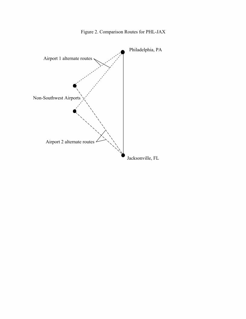
Figure 2. Comparison Routes for PHL-JAX

Philadelphia, PA

Jacksonville, FL

Non-Southwest Airports

Airport 1 alternate routes

Airport 2 alternate routes

Table 1. Probability of Southwest’s Entry into a Route

Southwest operates in one endpoint airport in the previous quarter (single presence)

0.004 (0.000)

Southwest operates in both endpoint airports in the previous quarter (dual presence)

0.238 (0.002)

N 135,111 Notes: The table shows estimates from a probit estimation for Southwest’s entry into a route in a particular quarter, conditional on the number of the route’s endpoint airports served by Southwest in the previous quarter. The excluded category includes observations where Southwest does not serve either endpoint airport in the previous quarter. Quarter fixed effects are included. Standard errors are in parentheses.

Table 2. Descriptive Statistics, Fare and Passenger Summaries

Mean (std deviation) Direct Flights to Threatened Airport

Avg. ln(fare) ln(passengers)

Number of Threatened Routes

Route-Carrier-Quarters in sample

Direct Flights to Neighboring Airport Avg. ln(fare)

ln(passengers)

Number of Threatened Routes Route-Carrier-Quarters in sample

5.21 (0.45) 2.55 (2.13)

678

18,969

5.16 (0.48) 3.81 (2.69)

169

7,296

Notes: Authors' calculations using the DB1A database from the U.S. Department of Transportation.

Table 3. Basic Results

(1) (2) (3) (4)

Dependent Variable: ln(P) ln(P) ln(Q) ln(Q)

Dual presence defined by: direct flight only any flight direct flight

only any flight

Operate both ends (no flights) (t-8 to t-7)

-.047 (.019)

-.037 (.050)

.017 (.037)

.042 (.055)


-.044 (.033)

-.010 (.039)

.000 (.051)

.006 (.059)


-.107 (.037)

-.073 (.042)

.129 (.055)

.129 (.058)


-.151 (.044)

-.097 (.050)

.125 (.085)

.061 (.075)

Operate both ends (no flights) (t)

-.187 (.051)

-.153 (.062)

.132 (.087)

.095 (.083)

Operate both ends (no flights) (t+1 to t+2)

-.189 (.051)

-.221 (.066)

.095 (.086)

.102 (.087)


-.260 (.055)

-.300 (.075)

.151 (.084)

.192 (.091)

Southwest Flying Route (t)

-.256 (.055)

-.185 (.071)

.118 (.100)

.066 (.087)

Southwest Flying Route (t+1 to t+2)

-.271 (.073)

-.226 (.070)

.115 (.100)

.067 (.099)


-.321 (.082)

-.234 (.076)

.142 (.115)

.118 (.106)

Route Carrier dummies Time Dummies

Y Y

Y Y

Y Y

Y Y

N 18,969 15,819 18,969 15,819 R2 .89 .84 .94 .93

Notes: This table shows estimates from passenger-weighted average logged fares and logged total passengers for our baseline sample. All regressions include route-carrier and quarter fixed effects. Standard errors are in parentheses and are clustered by route to account for correlation across time and across carriers on the same route. The sample includes all routes where Southwest threatens entry as defined in the text. The Operating Both Ends dummies denote Southwest having flights involving airports on both ends of a route previous to actually flying the route. The Southwest Flying Route dummies denote Southwest actually operating flights on the route. The number in parentheses denote the timing relative to the event happening (noted t in the table). Columns (1) and (3) define Southwest airlines as entering a route when they establish direct service between the two airports. Columns (2) and (4) define entry as establishing either direct or change-of-plane service, where the latter is defined as having in the sample at least 40 change-of-plane Southwest tickets for the route.

Table 4. Incumbent Average Fare Responses, Adjusted for Operating Cost Proxies

Dep.Var: ln(p) relative to (1)

(2) Alternates 1

(3) Alternates 2

(4) cost controls


-.047 (.019)

-.050 (.040)

-.036 (.029)

-.030 (.018)


-.044 (.033)

-.076 (.058)

-.026 (.041)

-.034 (.030)


-.107 (.037)

-.144 (.065)

-.093 (.048)

-.086 (.035)


-.151 (.044)

-.208 (.079)

-.164 (.052)

-.143 (.041)

Operate both ends (no flights) (t)

-.187 (.051)

-.237 (.083)

-.201 (.057)

-.176 (.049)


-.189 (.051)

-.235 (.085)

-.219 (.053)

-.162 (.043)


-.260 (.055)

-.257 (.095)

-.278 (.061)

-.222 (.047)

Southwest Flying Route -.256 (.055)

-.320 (.113)

-.290 (.072)

-.236 (.056)


-.271 (.073)

-.314 (.106)

-.333 (.081)

-.259 (.056)


-.321 (.082)

-.384 (.124)

-.378 (.095)

-.312 (.063)

Operating cost control, endpoint airport 1 - - .404

(.059) Operating cost control,

endpoint airport 2 - - .297 (.064)


Y Y

Y Y

Y Y

Y Y

N 18,969 17,239 18,498 18,146 R2 .89 .84 .87 .91

Notes: All regressions are weighted by passengers and include route-carrier and quarter fixed effects. Standard errors are in parentheses and are clustered by route to account for correlation across time and across carriers on the same route. The sample includes all routes where Southwest threatens entry as defined in the text. The Operating Both Ends dummies denote Southwest having flights involving airports on both ends of a route previous to actually flying the route. The Southwest Flying Route dummies denote Southwest actually operating flights on the route. The number in parentheses denote the timing relative to the event happening (noted t in the table). The dependent variable in columns (1) and (4) is the average log of fares for the route-carrier. The dependent variable in column (2) is the average log price of direct flights minus the price of direct flights by the same carrier between endpoint airport 1 and alternative airports that Southwest does not fly to. The dependent variable in column (3) is the price of direct flights on the route minus the price of direct flights by the same carrier between endpoint airport 2 and alternative airports that Southwest does not fly to. The operating cost controls are defined as average fares for the same carrier between the stated airport and cities that Southwest Airlines does not fly.

Table 5. Results by Type of Route

(1)

low HHI routes

(2) high HHI

routes

(3) ln(P)

nearby airport

(4) ln(Q)

nearby airport Operate Both Ends (No entry)

(t-8 to t-7) -.012 (.036)

-.054 (.024)

.017 (.043)

-.006 (.050)

Operate Both Ends (No entry) (t-6 to t-5)

.048 (.057)

-.056 (.026)

.123 (.054)

-.164 (.066)


.035 (.068)

-.122 (.027)

.101 (.057)

-.086 (.076)


.031 (.075)

-.167 (.036)

.132 (.064)

-.200 (.082)

Operate Both Ends (No entry) (t)

-.017 (.082)

-.202 (.045)

.076 (.051)

-.186 (.097)

Operate Both Ends (No entry) (t+1 to t+2)

-.051 (.085)

-.196 (.036)

.132 (.052)

-.225 (.105)


-.168 (.123)

-.266 (.044)

.170 (.076)

-.322 (.128)

Southwest Operating Route -.078 (.117)

-.270 (.059)

.176 (.071)

-.340 (.137)

Southwest Operating Route (t+1 to t+2)

-.122 (.107)

-.282 (.049)

.159 (.069)

-.302 (.133)


-.151 (.125)

-.333 (.052)

.170 (.077)

-.342 (.151)


Y Y

Y Y

Y Y

Y Y

N 9498 9200 7296 7296 R2 .86 .89 .88 .89

Notes: All regressions are weighted by passengers and include route-carrier and quarter fixed effects. Standard errors are in parentheses and are clustered by route to account for correlation across time and across carriers on the same route. The sample includes all routes where Southwest threatens entry as defined in the text. The Operating Both Ends dummies denote Southwest having flights involving airports on both ends of a route previous to actually flying the route. The Southwest Flying Route dummies denote Southwest actually operating flights on the route. The number in parentheses denote the timing relative to the event happening (noted t in the table). The dependent variable in columns (1), (2) and (3) is the average log of fares for the route-carrier. The dependent variable in (4) is the log number of passengers. Columns (1) and (2) divide the sample between routes that have HHI concentrations at or below the median in the sample and routes with HHI concentrations above the median. Columns (3) and (4) look at the price and quantity responses on routes to neighboring airports that Southwest does not fly to but are in the same market as an airport where Southwest does operate.

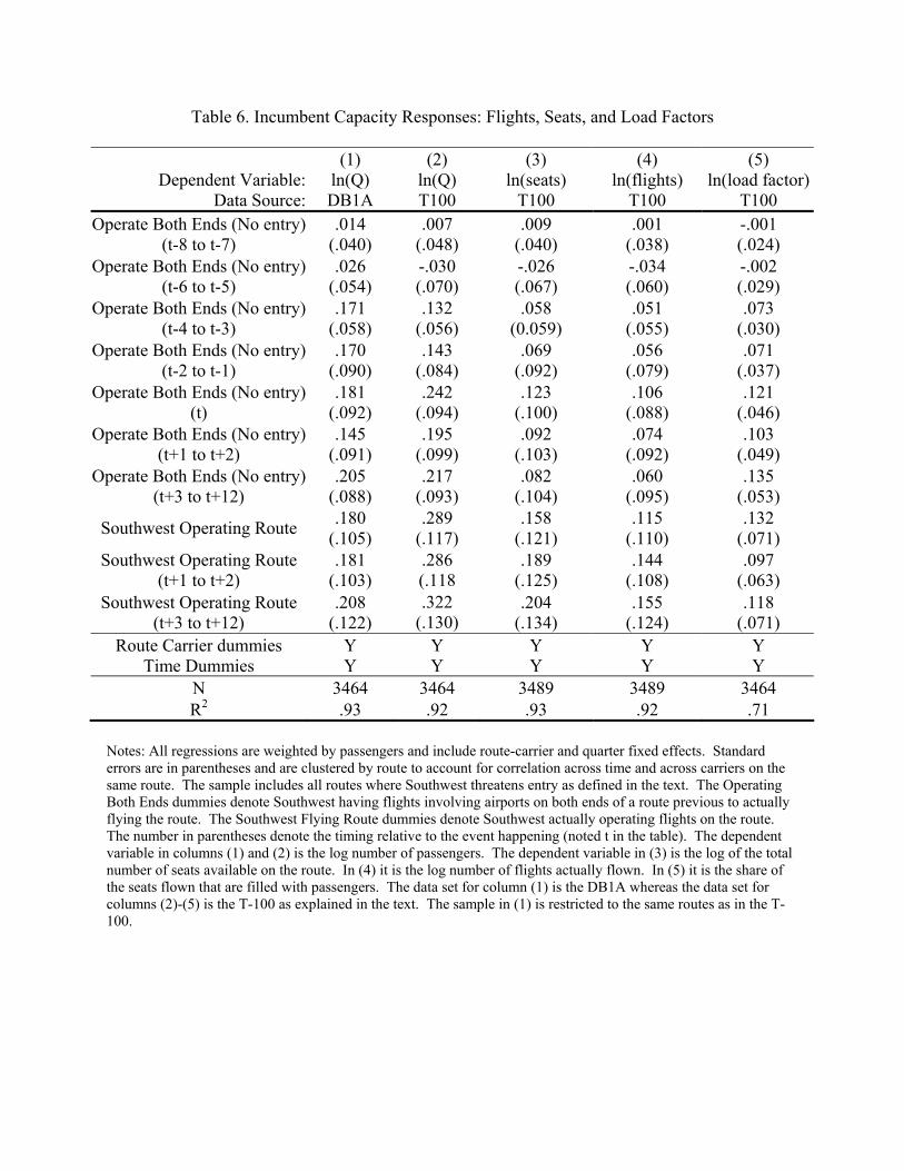
Table 6. Incumbent Capacity Responses: Flights, Seats, and Load Factors

Dependent Variable:

Data Source:

(1) ln(Q) DB1A

(2) ln(Q) T100

(3) ln(seats)

T100

(4) ln(flights)

T100

(5) ln(load factor)

T100 Operate Both Ends (No entry)

(t-8 to t-7) .014

(.040) .007

(.048) .009

(.040) .001

(.038) -.001 (.024)


.026 (.054)

-.030 (.070)

-.026 (.067)

-.034 (.060)

-.002 (.029)


.171 (.058)

.132 (.056)

.058 (0.059)

.051 (.055)

.073 (.030)


.170 (.090)

.143 (.084)

.069 (.092)

.056 (.079)

.071 (.037)


.181 (.092)

.242 (.094)

.123 (.100)

.106 (.088)

.121 (.046)


.145 (.091)

.195 (.099)

.092 (.103)

.074 (.092)

.103 (.049)


.205 (.088)

.217 (.093)

.082 (.104)

.060 (.095)

.135 (.053)

Southwest Operating Route .180 (.105)

.289 (.117)

.158 (.121)

.115 (.110)

.132 (.071)


.181 (.103)

.286 (.118

.189 (.125)

.144 (.108)

.097 (.063)


.208 (.122)

.322 (.130)

.204 (.134)

.155 (.124)

.118 (.071)


Y Y

Y Y

Y Y

Y Y

Y Y

N 3464 3464 3489 3489 3464 R2 .93 .92 .93 .92 .71

Notes: All regressions are weighted by passengers and include route-carrier and quarter fixed effects. Standard errors are in parentheses and are clustered by route to account for correlation across time and across carriers on the same route. The sample includes all routes where Southwest threatens entry as defined in the text. The Operating Both Ends dummies denote Southwest having flights involving airports on both ends of a route previous to actually flying the route. The Southwest Flying Route dummies denote Southwest actually operating flights on the route. The number in parentheses denote the timing relative to the event happening (noted t in the table). The dependent variable in columns (1) and (2) is the log number of passengers. The dependent variable in (3) is the log of the total number of seats available on the route. In (4) it is the log number of flights actually flown. In (5) it is the share of the seats flown that are filled with passengers. The data set for column (1) is the DB1A whereas the data set for columns (2)-(5) is the T-100 as explained in the text. The sample in (1) is restricted to the same routes as in the T-100.

Table 7. Frequent Flyers and the Fare Declines

(1)

ln(P) 25th pctile

(2) ln(P)

50th pctile

(3) ln(P)

75th pctile

(4) low FF

likelihood

(5) high FF

likelihood Operate Both Ends (No entry)

(t-8 to t-7) -.043 (.021)

-.066 (.025)

-.048 (.032)

.056 (.040)

-.050 (.020)


-.059 (.026)

-.079 (.038)

-.011 (.045)

.122 (.079)

-.050 (.033)


-.100 (.028)

-.168 (.045)

-.151 (.060)

.103 (.103)

-.113 (.038)


-.127 (.034)

-.189 (.057)

-.205 (.070)

.043 (.109)

-.157 (.044)


-.157 (.039)

-.227 (.064)

-.241 (.084)

-.076 (.103)

-.189 (.051)


-.173 (.044)

-.233 (.067)

-.237 (.082)

-.070 (.109)

-.191 (.051)


-.220 (.053)

-.280 (.075)

-.333 (.097)

-.106 (.113)

-.265 (.056)

Southwest Operating Route -.177 (.056)

-.263 (.074)

-.311 (.091)

-.177 (.118)

-.256 (.056)


-.207 (.084)

-.299 (.100)

-.310 (.110)

-.175 (.120)

-.272 (.075)


-.300 (.075)

-.353 (.101)

-.323 (.127)

-.192 (.123)

-.326 (.083)


Y Y

Y Y

Y Y

Y Y

Y Y

N 18,968 18,968 18,968 9518 9382 R2 .81 .79 .82 .86 .89

Notes: All regressions are weighted by passengers and include route-carrier and quarter fixed effects. Standard errors are in parentheses and are clustered by route to account for correlation across time and across carriers on the same route. The sample includes all routes where Southwest threatens entry as defined in the text. The Operating Both Ends dummies denote Southwest having flights involving airports on both ends of a route previous to actually flying the route. The Southwest Flying Route dummies denote Southwest actually operating flights on the route. The number in parentheses denote the timing relative to the event happening (noted as t in the table). Columns (1)-(3) present quantile regressions for the 25th, 50th and 75th percentiles or prices on a route. The dependent variable in columns (4) and (5) is the average log of fares for the route-carrier. These columns divide the sample according to whether the routes involve airports where the carrier has less or more than the median share of the total domestic traffic.

how do incumbents respond to the threat of entry? · pdf fileit uses a case study from the...

Documents