how does bayesian knowledge tracing model emergence of
TRANSCRIPT

How Does Bayesian Knowledge Tracing Model Emergence of Knowledge about a Mechanical System?
Hee-Sun Lee University of California, Santa Cruz
1156 High Street Santa Cruz, CA 95064
1-831-459-2326
Robert Tinker The Concord Consortium
25 Love Lane Concord, MA 01742
1-978-405-3225
Nathan Kimball The Concord Consortium
25 Love Lane Concord, MA 01742
1-978-405-3225
Gey-Hong Gweon University of California, Santa Cruz
1156 High Street Santa Cruz, CA 95064
1-831-459-1806
William Finzer The Concord Consortium West 6550 Vallejo Street, Suite 101C
Emeryville, CA 94608 1-510-984-4380
Amy Pallant
The Concord Consortium 25 Love Lane
Concord, MA 01742 1-978-405-3227
Chad Dorsey The Concord Consortium
25 Love Lane Concord, MA 01742
1-978-405-3200
Daniel Damelin The Concord Consortium
25 Love Lane Concord, MA 01742
1-978-405-3242
Trudi Lord The Concord Consortium
25 Love Lane Concord, MA 01742
1-978-405-3221
ABSTRACT
An interactive learning task was designed in a game format to
help high school students acquire knowledge about a simple
mechanical system involving a car moving on a ramp. This ramp
game consisted of five challenges that addressed individual
knowledge components with increasing difficulty. In order to
investigate patterns of knowledge emergence during the ramp
game, we applied the Monte Carlo Bayesian Knowledge Tracing
(BKT) algorithm to 447 game segments produced by 64 student
groups in two physics teachers' classrooms. Results indicate that,
in the ramp game context, (1) the initial knowledge and guessing
parameters were significantly highly correlated, (2) the slip
parameter was interpretable monotonically, (3) low guessing
parameter values were associated with knowledge emergence
while high guessing parameter values were associated with
knowledge maintenance, and (4) the transition parameter showed
the speed of knowledge emergence. By applying the k-means
clustering to ramp game segments represented in the three
dimensional space defined by guessing, slip, and transition
parameters, we identified seven clusters of knowledge emergence.
We characterize these clusters and discuss implications for future
research as well as for instructional game design.
Categories and Subject Descriptors
H. 2. 8. [Database Management]: Database Applications - Data
mining; K.3.1 [Computers and Education]: Computer Uses in
Education - Computer-assisted instruction (CAI)
General Terms
Algorithms, Performance, Design, Experimentation, Verification.
Keywords
Bayesian Knowledge Tracing, Physics Learning, Game-Based
Learning.
1. INTRODUCTION For meaningful and enduring science learning, students need to be
actively engaged with the knowledge generation process [1-3].
Games and simulations have been used to facilitate such
engagement [4]. Computer-based games and simulations are built
upon technological platforms where automatic logging of
students' actions is increasingly possible. Combined with the rapid
rise in computing power and advances in machine-learning
algorithms [5, 6], it is thought that research can be carried out to
investigate student learning moment-by-moment and document
how changes at the microgenetic level occur in students' cognition
[7, 8]. Despite this potential, data mining and learning analytics
are yet to be fully integrated in most science learning
environments [8] beyond intelligent tutoring systems [9, 10] and a
few applications in curriculum systems [11] and assessment
Permission to make digital or hard copies of all or part of this work
for personal or classroom use is granted without fee provided that
copies are not made or distributed for profit or commercial
advantage and that copies bear this notice and the full citation on
the first page. Copyrights for components of this work owned by
others than ACM must be honored. Abstracting with credit is
permitted. To copy otherwise, or republish, to post on servers or to
redistribute to lists, requires prior specific permission and/or a fee.
Request permissions from [email protected].
LAK ’15, March 16-20, 2015, Poughkeepsie, NY, USA. Copyright 2015 ACM 978-1-4503-3417-4...$15.00.
http://dx.doi.org/10.1145/2723576.2723587

systems [6, 12]. With this new opportunity, learning scientists are
cautiously exploring various methods related to data mining and
learning analytics as part of their research on how learning occurs
[8].
One of the popular algorithms to trace students' knowledge
growth over time is Bayesian Knowledge Tracing (BKT). BKT
models student learning of a knowledge component as a
monotonically increasing function of which shape is determined
by initial knowledge (Li), guessing (G), slip (S), and transition (T)
parameters [13]. The latent knowledge growth plots resulting
from the BKT analysis have been utilized heavily in intellectual
tutoring systems to represent students' knowledge growth during
learning tasks. Variants of the original BKT [13] have been
developed in order to (1) reduce errors in parameter estimations
[14], (2) account for effective supports [15], and (3) pinpoint
exact episodes of knowledge acquisition [16]. While most BKT
research applied to intelligent tutoring systems is directed at
defining uniquely and accurately the latent knowledge growth
curve from available student performance information, less
attention has been devoted to interpreting the four BKT parameter
estimates in the context of learning and establishing student
learning patterns based on these parameters.
In this study, we designed an instructional game in an
environment called Common Online Data Analysis Platform
(CODAP) where students conducted simulation-based
experiments on a ramp system, analyzed data using built-in tables
and graphs, and identified patterns in the data sets. Students'
actions within CODAP and resulting performance scores were
logged automatically in the background. This study applied the
BKT algorithm to trace how students' knowledge about a simple
mechanical system involving a car on a ramp emerged over time.
We investigated what knowledge emergence patterns could be
extracted from BKT parameter estimates.
2. METHODS
2.1 Subjects The ramp game was implemented in eight physics classrooms
taught by two teachers in two high schools located in the
Northeastern part of the United States. A total of 164 students,
working in 64 groups, participated in this study. Each student
group consisted of two to three students with mixed genders.
Among the students, 49% were male and 51% were female; 38%
were in the 9th grade, 30% were in the 11th grade, and 31% were
in the 12th grade. Students' physics abilities were mixed as they
were sampled from both AP and introductory physics classes. The
ramp game was carried out over two class periods.
2.2 Ramp Game Design Students typically acquire knowledge about multivariate
relationships associated with a mechanical system by
manipulating equations and formulas. In contrast, the ramp game
was designed to help students use data shown in tables and graphs
to recognize relationships among the variables involved in a ramp
system. Figure 1 shows four variables related to the motion of a
car on a ramp:
Distance to the Right (outcome variable)
Start Height (changed by dragging the car on the ramp)
Car Mass (set by the game)
Friction (set by the game in Challenges 1 - 4, and by the
student with a slider in Challenge 5)
The movement of the car on the ramp can be influenced by some
of these variables. It is the job of the student to determine how to
set the parameters so that the car can stop within a target area.
When the Start button is pressed, the car accelerates down the
ramp and then moves along a horizontal line until it stops under
the influence of friction. For Challenges 1 - 4, students set the
variable of Start Height. For the 5th challenge, the Start Height
variable is fixed and students must vary the car's friction.
For each simulation run, the variables of input and output are
transferred to a CODAP case table. A graph showing the Start
Height (x-axis) vs. End Distance (y-axis) is displayed next to the
game. The game provides feedback as well as a score after each
run, prompting students to use the graph data to create strategies
to succeed in the challenges more quickly and precisely. Strategic
use of the data table and the graph allows quicker game play and a
higher score. There are five challenges, each of which contains 3
to 6 steps. If students come close to or hit the center of the target,
they move to the next step within the same challenge where the
size of the target shrinks. Each of the five challenges addresses a
different knowledge component. The higher the challenge, the
more difficult the knowledge component addressed in the
challenge:
Challenge 1 (3 steps): point-to-point relationship between a
starting height and a fixed landing location when friction is
fixed;
Challenge 2 (4 steps): positive linear relationship between
starting height and landing location;
Challenge 3 (4 steps): positive linear relationship between
starting height and landing location when friction changes;
Challenge 4 (3 steps): no dependence of mass on positive
linear relationship between starting height and landing
location when friction is fixed;
Challenge 5 (6 steps): inverse relationship between friction
and landing location when starting height and mass are
fixed.
2.3 Game Scoring Every simulation run is worth 100 points. The student’s score is
100 only if the car stops at the center of the target—an antenna
centered on the car must align with a vertical hash mark on the
target. The score, rounded to five points, goes down away from
the center as a cosine, dropping to 50 halfway to the edge of the
target and zero at the edge of the target. As the steps increase
within each challenge, the target shrinks. This makes it harder to
get a high score. If the student is more than twice the distance
from the center to the edge, the software counts this as a random
guess. If the student gets more than 67 points at one step, he/she
goes on to the next step. If the step just completed was the last
step in a challenge, the student is promoted to the first step of the
next challenge. If the student gets less than 25 points and the
failed step is not the first in a challenge, he/she goes back a step.
If it was the first, the student repeats the first step.
2.4 BKT Analysis Logging data for this study was collected from all 64 student
groups. We segmented the logged data by challenge, resulting in
447 game segments. We applied the BKT algorithm to these
segments. Below are the four parameters of a BKT model [13]:
Initial knowledge parameter associated with the
probability that the student already knows the target
knowledge prior to a simulation run;
Guessing parameter associated with the
probability of guessing correctly without the target
knowledge (i.e., false positive);
Slip parameter associated with the probability of
making a mistake when the student has the target
knowledge (i.e., false negative);
Transition parameter associated with the
probability of becoming knowledgeable at a given game
segment.
In the literature, various approaches for parameter optimization
have been attempted, including a brute force approach of making
a four-dimensional grid, evaluating all values on the grid, and
finding a set of parameters that minimizes the error of estimation.
This is equivalent to minimizing “residuals" [5, 6]. Instead, we
combined a Monte Carlo sampling of the parameter space with the
well-known Levenberg-Marquardt algorithm for the non-linear
least squares fit to find a set of parameters that best fit the data
[15].
3. Results The logged data analyzed in this study were 91,112 lines long,
and the size of the logged data file was 13MB. An average
number of logged lines per student group was 1,423. Among the
447 game segments, 381 (85.2%) were fit for BKT analysis. All
of the 66 segments unfit for BKT had three or less data points.
Note that, because BKT estimates four parameters, three data
points are not sufficient to yield four stable BKT parameter
estimates.
3.1 Clustering in (G, S, T) Space We used the k-means method to identify clusters that might be
present in the (G, S, T) space. We omitted the initial knowledge
parameter, Li, because it was significantly, positively, and
strongly correlated with G. See Table 1.
Table 1. Correlations among BKT Parameters
Li G S T
Li -- .71*** -.08 -.04
G -- .27*** -.06
S -- -.19***
T --
Note: *** p < .001.
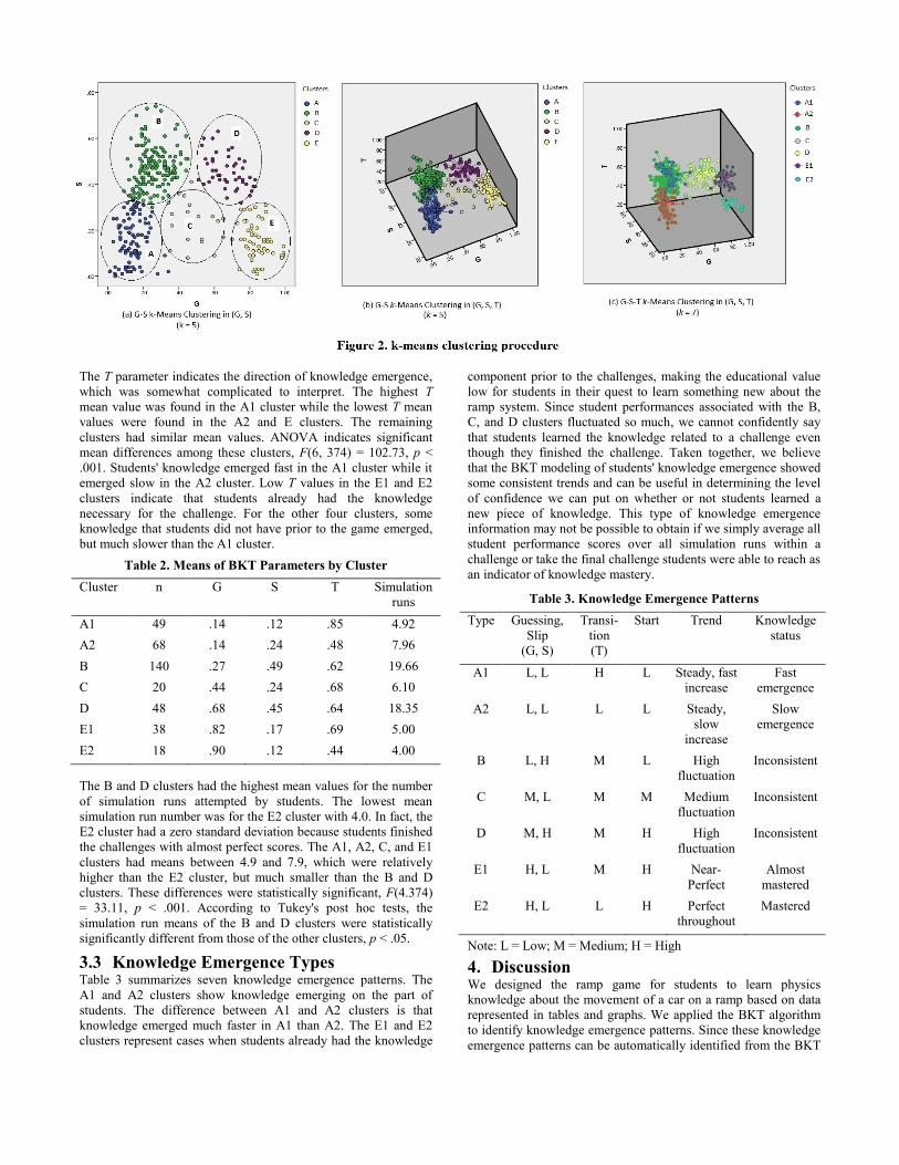
To determine an appropriate k-value, i.e., the number of clusters,
we relied on our observations of scatter plots in the G, S, and T
parameter space. Figure 2 shows how we determined the k-value
as seven. First, we created a scatter plot between G and S. See
Figure 2(a). On this graph, it was apparent that the data points
were not uniformly distributed over the entire ranges on both
axes. Instead, there were five identifiable clusters, from A to E.
Then, we inspected how the five clusters were spread in the (G, S,
T) space. See Figure 2(b). This three-dimensional scatter plot
indicated that the A and E clusters had dumbbell shape
distributions along the T-axis unlike the B, C, and D clusters. We
thus divided the A cluster into A1 with higher T values and A2
with lower T values, as well as the E cluster into E1 with higher T
values and E2 with lower T values. As a result, we noticed seven
clusters in the (G, S, T) space. We then applied the k-means
clustering algorithm using SPSS with k = 7, resulting in Figure
2(c). Table 2 shows the descriptive statistics of these seven
clusters.
3.2 Cluster Characteristics Among the BKT-analyzed segments, the largest majority
belonged to the B cluster (36.7% of the total), followed by the A2
and A1 clusters. The E2 and C clusters had the smallest numbers
of segments. With the seven identified clusters in the (G, S, T)
space, we compared distributions of G, S, and T parameters across
clusters. For the G parameter, the mean G values were the lowest
for A1 and A2 clusters and gradually increased from B, C, D, E1,
to E2 clusters. According to ANOVA, the means of these seven
clusters were significantly different from one another, except the
A1 and A2 clusters, F(6, 374) = 765.84, p < .001.
For the S parameter, the A1, E1, and E2 clusters had lower mean
values while the B and D clusters had higher values. The A2 and
C clusters had medium values. In fact, ANOVA indicates that
mean S values were statistically significantly different (A1, E1,
E2 << A2, C << B, D), F(6, 374) = 176.58, p < .001. This means
that segments in the A1, E1, and E2 clusters did not have many
mistakes towards the end of the challenge while those in the B and
D clusters had more mistakes made by students towards the end.
The T parameter indicates the direction of knowledge emergence,
which was somewhat complicated to interpret. The highest T
mean value was found in the A1 cluster while the lowest T mean
values were found in the A2 and E clusters. The remaining
clusters had similar mean values. ANOVA indicates significant
mean differences among these clusters, F(6, 374) = 102.73, p <
.001. Students' knowledge emerged fast in the A1 cluster while it
emerged slow in the A2 cluster. Low T values in the E1 and E2
clusters indicate that students already had the knowledge
necessary for the challenge. For the other four clusters, some
knowledge that students did not have prior to the game emerged,
but much slower than the A1 cluster.
Table 2. Means of BKT Parameters by Cluster
Cluster n G S T Simulation
runs
A1 49 .14 .12 .85 4.92
A2 68 .14 .24 .48 7.96
B 140 .27 .49 .62 19.66
C 20 .44 .24 .68 6.10
D 48 .68 .45 .64 18.35
E1 38 .82 .17 .69 5.00
E2 18 .90 .12 .44 4.00
The B and D clusters had the highest mean values for the number
of simulation runs attempted by students. The lowest mean
simulation run number was for the E2 cluster with 4.0. In fact, the
E2 cluster had a zero standard deviation because students finished
the challenges with almost perfect scores. The A1, A2, C, and E1
clusters had means between 4.9 and 7.9, which were relatively
higher than the E2 cluster, but much smaller than the B and D
clusters. These differences were statistically significant, F(4.374)
= 33.11, p < .001. According to Tukey's post hoc tests, the
simulation run means of the B and D clusters were statistically
significantly different from those of the other clusters, p < .05.
3.3 Knowledge Emergence Types Table 3 summarizes seven knowledge emergence patterns. The
A1 and A2 clusters show knowledge emerging on the part of
students. The difference between A1 and A2 clusters is that
knowledge emerged much faster in A1 than A2. The E1 and E2
clusters represent cases when students already had the knowledge
component prior to the challenges, making the educational value
low for students in their quest to learn something new about the
ramp system. Since student performances associated with the B,
C, and D clusters fluctuated so much, we cannot confidently say
that students learned the knowledge related to a challenge even
though they finished the challenge. Taken together, we believe
that the BKT modeling of students' knowledge emergence showed
some consistent trends and can be useful in determining the level
of confidence we can put on whether or not students learned a
new piece of knowledge. This type of knowledge emergence
information may not be possible to obtain if we simply average all
student performance scores over all simulation runs within a
challenge or take the final challenge students were able to reach as
an indicator of knowledge mastery.
Table 3. Knowledge Emergence Patterns
Type Guessing,
Slip
(G, S)
Transi-
tion
(T)
Start Trend
Knowledge
status
A1 L, L H L Steady, fast
increase
Fast
emergence
A2 L, L L L Steady,
slow
increase
Slow
emergence
B L, H M L High
fluctuation
Inconsistent
C M, L M M Medium
fluctuation
Inconsistent
D M, H M H High
fluctuation
Inconsistent
E1 H, L M H Near-
Perfect
Almost
mastered
E2 H, L L H Perfect
throughout
Mastered
Note: L = Low; M = Medium; H = High
4. Discussion We designed the ramp game for students to learn physics
knowledge about the movement of a car on a ramp based on data
represented in tables and graphs. We applied the BKT algorithm
to identify knowledge emergence patterns. Since these knowledge
emergence patterns can be automatically identified from the BKT
parameter estimates, we expect that next steps would be to use
this information to create scaffolds to guide students' further
knowledge development.
To apply BKT similarly to what we did in our research, learning
tasks should be designed as follows: (1) a knowledge construct is
defined as a collection of increasingly difficult knowledge
components, (2) a series of learning tasks are designed in such a
way that each learning task addresses a knowledge component
from easy to difficult, (3) each learning task engages students to
produce four or more simulation trials, and (4) student
performance is quantified to indicate student success on each
learning task. We developed a scoring method to reward students'
accurate predictions on a 100-point scale, which was very
sensitive to student success as compared to binary scores that
were conventionally used in intellectual tutoring systems.
The most interpretable BKT parameter appeared to be the slip
parameter, S, because the mastery (emergence) of knowledge was
associated with low S values while inconsistent learning was
associated with high S in our research. In terms of whether or not
a knowledge component was mastered, the guessing parameter, G,
appeared to be bidirectional because both very low and very high
G values were associated with students' learning or having
mastered the knowledge component while medium G values were
associated with inconsistent learning.
Even though the ramp game was designed to follow knowledge
emergence, we encountered several difficulties in applying BKT
to our data. First, tracing student learning in real-world classroom
settings was not straightforward. In particular, marking the
beginning and the ending of a student group's work from the
logged data was difficult because (1) students were often engaged
with multiple learning tasks during class, (2) student group
memberships changed from class to class, and (3) students started,
stopped, and restarted the ramp game on their own or by the
teacher or for unknown reasons. Stringing all relevant ramp game
segments per group was extremely challenging. This may not be
seen in laboratory-based settings or assessment settings. Smart
logging technologies may be necessary to handle these types of
difficulties in automatically identifying and connecting segments
belonging to the same learning event of interest.
Generalizability of our findings is limited due to the student
sample, which was not drawn randomly from the general
population and was relatively small in size. The knowledge
emergence patterns found in this research can be due to the type
of learning task developed in this study. Additional research is
necessary to confirm or expand the knowledge emergence patterns
we identified in this paper.
Our next research step involves triangulation of knowledge
emergence patterns with other sources of student learning data
such as (1) videos we collected on a smaller set of student groups
working on the ramp game, (2) students' written reflections on the
strategies they used for the challenge, and (3) student pre-post test
performance on how students used tables and graphs to
investigate mechanical systems. Taken together, we can explore
other exciting analytic possibilities with the BKT algorithm to
capture student learning in real-world classroom settings.
5. ACKNOWLEDGMENTS This material is based upon work supported by the National
Science Foundation under grants IIS-1147621 and DRL-1435470.
Any opinions, findings, conclusions or recommendations
expressed in this material are those of the authors and do not
necessarily reflect the views of the National Science Foundation.
6. REFERENCES [1] National Research Council, National science education
standards. Washington, DC: National Academies Press,
1996.
[2] National Research Council, Taking science to school.
Washington, DC: National Academies Press, 2007.
[3] National Research Council, A framework for K-12 science
education: Practices, crosscutting concepts, and core ideas.
Washington, DC: National Academies Press, 2012.
[4] M. A. Honey and M. Hilton, Learning science through
computer games and simulations. Washington D.C.: The
National Academies Press, 2011.
[5] J. Gobert, M. Sao Pedro, R. Baker, E. Toto, and O.
Montalvo, "Leveraging educational data mining for real time
performance assessment of scientific inquiry skills within
microworlds," Journal of Educational Data Mining, vol. 4,
pp. 111-143, 2012.
[6] J. Gobert, M. Sao Pedro, J. Raziuddin, and R. Baker, "From
log files to assessment metrics for science inquiry using
educational data mining," Journal of the Learning Sciences,
vol. 22, pp. 521-563, 2013.
[7] D. Kuhn, "Microgenetic study of change: What has it told
us?," Psychological Science, vol. 6, pp. 133-139, 1995.
[8] T. Martin and B. Sherin, "Learning analytics and
computational techniques for detecting and evaluating
patterns in learning: An introduction to the special issue,"
Journal of the Learning Sciences, vol. 22, pp. 511-520, 2013.
[9] J. R. Anderson, C. F. Boyle, A. Corbett, and M. W. Lewis,
"Cognitive modeling and intelligent tutoring," Artificial
Intelligence, vol. 42, 1990.
[10] D. C. Merrill, B. J. Reiser, M. Ranney, and J. G. Trafton,
"Effective tutoring techniques: A comparison of human
tutors and intelligent tutoring systems," Journal of the
Learning Sciences, vol. 2, pp. 277-305, 1992.
[11] J. L. Davernport, A. Raffety, M. J. Timms, D. Yaron, and M.
Karabinos, "ChemVLab+: Evaluating a virtual lab tutor for
high school chemistry," in International Conference of the
Learning Sciences, 2012, pp. 381-385.
[12] E. S. Quellmalz, M. J. Timms, M. D. Silberglitt, and B. C.
Buckley, "Science assessments for all: Integrating science
simulations into balanced state science assessment systems,"
Journal of Research in Science Teaching, vol. 49, pp. 363-
393, 2012.
[13] A. Corbett and J. Anderson, "Knowledge-tracing: Modeling
the acquisition of procedural knowledge," User Modeling
and User Adopted Interaction, vol. 4, pp. 253-278, 1995.
[14] R. Baker, A. T. Corbett, I. Roll, and K. R. Koedinger, "More
accurate student modeling through contextual estimation of
slip and guess probabilities in Bayesian Knowledge
Tracing," in Proceedings of the 9th International Conference
on Intelligent Tutoring Systems, 2008, pp. 406-415.
[15] J. E. Beck, K. Chang, J. Mostow, and A. Corbett, "Does help
help? Introducing the Bayesian evaluation and assessment
methodology," in Proceedings of the 9th International
Conference on Intelligent Tutoring Systems, 2008, pp. 383-
394.
[16] R. Baker, A. Hershkovitz, L. M. Rossi, A. B. Goldstein, and
S. M. Gowda, "Predicting robust learning with the visual
form of the moment-by-moment learning curve," Journal of
the Learning Sciences, vol. 22, pp. 639-666, 2013.