NBER WORKING PAPER SERIES

HOW DOES HOUSEHOLD SPENDING RESPOND TO AN EPIDEMIC? CONSUMPTIONDURING THE 2020 COVID-19 PANDEMIC

Scott R. BakerR.A. FarrokhniaSteffen MeyerMichaela Pagel

Constantine Yannelis

Working Paper 26949http://www.nber.org/papers/w26949

NATIONAL BUREAU OF ECONOMIC RESEARCH1050 Massachusetts Avenue

Cambridge, MA 02138April 2020

The authors wish to thank Sylvain Catherine, Caroline Hoxby, Ralph Koijen, Amir Sufi, Pietro Veronesi,Rob Vishny and Neil Ning Yu for helpful discussions and comments. Constantine Yannelis is gratefulto the Fama Miller Center for generous financial support. R.A. Farrokhnia is grateful to AdvancedProjects and Applied Research in Fintech at Columbia Business School for support. We are gratefulto Suwen Ge, Sypros Kypraios, Sharada Sridhar, George Voulgaris and Jun Xu for excellent researchassistance. This draft is preliminary and comments are welcome. The views expressed herein are thoseof the authors and do not necessarily reflect the views of the National Bureau of Economic Research.

NBER working papers are circulated for discussion and comment purposes. They have not been peer-reviewed or been subject to the review by the NBER Board of Directors that accompanies officialNBER publications.

© 2020 by Scott R. Baker, R.A. Farrokhnia, Steffen Meyer, Michaela Pagel, and Constantine Yannelis.All rights reserved. Short sections of text, not to exceed two paragraphs, may be quoted without explicitpermission provided that full credit, including © notice, is given to the source.

How Does Household Spending Respond to an Epidemic? Consumption During the 2020COVID-19 PandemicScott R. Baker, R.A. Farrokhnia, Steffen Meyer, Michaela Pagel, and Constantine YannelisNBER Working Paper No. 26949April 2020JEL No. D14,E21,G51

ABSTRACT

We explore how household consumption responds to epidemics, utilizing transaction-level householdfinancial data to investigate the impact of the COVID-19 virus. As the number of cases grew, householdsbegan to radically alter their typical spending across a number of major categories. Initially spendingincreased sharply, particularly in retail, credit card spending and food items. This was followed bya sharp decrease in overall spending. Households responded most strongly in states with shelter-in-placeorders in place by March 29th. We explore heterogeneity across partisan affiliation, demographicsand income. Greater levels of social distancing are associated with drops in spending, particularlyin restaurants and retail.

Scott R. BakerKellogg School of ManagementNorthwestern University2211 Campus DriveEvanston, IL 60208and NBERs-baker@kellogg.northwestern.edu

R.A. FarrokhniaColumbia Graduate School of Business3022 BroadwayNew York, NY 10027farrokhnia@gsb.columbia.edu

Steffen MeyerUniversity of Southern DenmarkCampusvej 555230 Odense MDenmarkstme@sam.sdu.dk

Michaela PagelColumbia Business School3022 BroadwayUris HallNew York, NY 10027and NBERmpagel@columbia.edu

Constantine YannelisBooth School of BusinessUniversity of Chicago5807 S. Woodlawn AvenueChicago, IL 60637and NBERconstantine.yannelis@chicagobooth.edu

1 Introduction

Disease epidemics have plagued human societies since at least the earliest days of recorded his-

tory. This paper presents the first study of how households’ consumption and debt respond to an

outbreak using transaction-level household data. As COVID-19 began to spread across the United

States in March 2020, households across the country were faced with drastic changes in many as-

pects of their lives. Large numbers of businesses were closed by government decree and in many

cities and states, Americans were required to limit trips outside and exposure to others following

shelter-in-place orders.

While Americans adjusted how they lived and worked in response to uncertainty about how

the future would play out, they also rapidly altered how and where they spent their money. This

paper works to deploy transaction-level household financial data to provide a better and more

comprehensive understanding of how households shifted spending as news about the virus spread

and the impact in a given geographic area became more severe and far-reaching.

The extent to which both individual households as well as the economy at large have been

upended is without recent precedent. Entire industries and cities were largely shut down, with

estimates of the decline in economic activity hitting all-time records. Policymakers at all levels of

government and across a wide range of institutions have worked to mitigate the economic harm

on households and small businesses. However, the speed at which the economic dislocation is

occurring has made it difficult for policymakers to properly target fiscal stimuli to households

and credit provision to businesses. After all, little is known about how households respond in

their spending to a pandemic on a scientific basis and across a larger number of households and

geographies.

This paper aims to close this gap by utilizing transaction-level household financial data to

analyze the impact of the COVID-19 outbreak on the spending behavior of tens of thousands

of Americans. We use transaction-level data from linked bank-accounts from a non-profit that

works with individuals to sustain savings habits. Transaction-level financial data of this type is

a useful tool for understanding household financial behavior in great detail. In the context of the

current COVID-19 outbreak, it can allow for a high speed, dynamic and timely diagnosis of how

households have adjusted their spending, when they began to respond, and what the characteristics

2

are of the households who have responded the fastest and strongest.1

News media reported that customers emptied supermarket shelves in an effort to stock-pile

durable goods.2 Furthermore, as advice flowed from federal and state governments to households,

one common refrain was that households should prepare to mostly stay inside their homes for

multiple weeks with minimal trips outside. Home production is thus a source of savings that

households can engage in which should also increase their spending at certain stores as opposed to

others.

We find that households substantially changed their spending as news about the COVID-19’s

impact in their area spread. Overall, spending increased dramatically in an attempt to stockpile

needed home goods and also in anticipation of the inability to patronize retailers. Household

spending increases by approximately 50% overall between February 26 and March 11. Grocery

spending remains elevated through March 27, with a 7.5% increase relative to earlier in the year.

We also see an increase in card spending, which is consistent with households borrowing to stock-

pile goods. As the virus spread and more households stayed home, we see sharp drops in restau-

rants, retail, air travel and public transport in mid to late March.

Restaurant spending declined by approximately one third. The speed and timing of these in-

creases in spending varied significantly across individuals depending on their geographic location

as state and local governments reacted to outbreaks of different sizes and with different levels of

urgency. The overall drop in spending is approximately twice as large in states that issued shelter-

in-place orders, however the increase in grocery spending is three times as large for states with

shelter-in-place orders.

We explore heterogeneity among partisan affiliations and demographics, which are closely tied

to stated beliefs about the impacts of the new virus. Republicans generally reported less concern

about the new virus. For example, an Axios Poll between March 5 and 9 found that 62% of

Republicans thought that the COVID-19 threat was greatly exagerated, while 31% of Democrats

and 35% of Independents thought the same. A Quinnipac poll between March 5 and 8 also found

that 68% of Democrats were concerned, while only 35% of Republicans were concerned. Contrary

1Researchers have previously utilized a range of transaction-level household financial datasets to answer questionsabout household consumption, liquidity, savings, and investment decisions. See Baker (2018), Baker and Yannelis(2017), Olafsson and Pagel (2018), Baker, Kueng, Meyer and Pagel (2020), and Meyer and Pagel (2019).

2For example, see USA Today, CNN, and FoxNews.

3

to much of what was seen in the press, and despite lower levels of observed social distancing,

Republicans actually spent more than Democrats in the early days of the epidemic. We see some

significant differences in categorical responses, with Republicans spending more at restaurants and

in retail shops, which is consistent with lower levels of concern about the virus or differential risk

exposure.

We see significant heterogeneity along demographic characteristics, but little along household

income. Households with children stockpiled more, and men stockpiled less in early days as the

virus was spreading. We find more spending in later periods by the young. We see little hetero-

geneity across income, which is largely consistent with work by Kaplan, Violante and Weidner

(2014) and Kaplan and Violante (2014) and the “wealthy-hand-to-mouth."

This paper joins a large literature on household consumption. Early empirical work, such as

Zeldes (1989), Souleles (1999), Pistaferri (2001), Johnson, Parker and Souleles (2006), Blundell,

Pistaferri and Preston (2006) and Agarwal, Liu and Souleles (2007) used survey data or studied

tax rebates. Gourinchas and Parker (2002), Kaplan and Violante (2010) and Kaplan and Violante

(2014) provide theoretical models of household consumption responses. Recent work uses admin-

istrative data (Fuster, Kaplan and Zafar, 2018; Di Maggio, Kermani, Keys, Piskorski, Ramcharan,

Seru and Yao, 2017) and Baker (forthcoming), Pagel and Vardardottir (forthcoming) and Baker

and Yannelis (2017) have studied income shocks and consumption using financial aggregator data.

Jappelli and Pistaferri (2010) provide a review of this literature.

This paper is the first to study how household spending reacts in an epidemic, where there are

anticipated income shocks as well as the threat of supply chain disruption, but all combined with

significant uncertainty. In early March, there was little direct effect of COVID-19 in the United

States, but significant awareness of potential damage in the future. We see significant stockpiling

and spending reactions, which is consistent with expectations playing a large role in household

consumption decisions.

This paper also relates to a literature on how crises impact the economy, and policy responses to

those crises. In the aftermath of the 2008 Great Recession, a large body of work studied how credit

supply shocks (Mian and Sufi, 2009, 2011; Mian, Rao and Sufi, 2013) and securitization (Keys,

Mukherjee, Seru and Vig, 2008; Keys, Seru and Vig, 2012) led to the financial crisis. Several

papers also study the effect of government policies aimed at mitigating the effects of the financial

4

crisis. (Bhutta and Keys, 2016; Di Maggio, Kermani, Keys, Piskorski, Ramcharan, Seru and Yao,

2017; Ganong and Noel, 2018). This paper provides a first look at the impacts of the new epidemic

on households, which will be key in evaluating any future policy response.

Additionally, the paper joins a growing literature in finance on the impacts of how belief het-

erogeneity shaped by partisan politics affects real economic decisions. Malmendier and Nagel

(2011) show the individuals growing up in the Great Depression exhibited more risk averse behav-

ior relative to others. The literature on how partisanship affects economic decisions has had mixed

findings. Some papers have found large effects of partisanship on economic decision-making.

For example, Kempf and Tsoutsoura (2018) explore how partisanship affects financial analysts

decisions and Meeuwis, Parker, Schoar and Simester (2018) find large effects of the 2016 US

Presidential election on portfolio rebalancing. Mian, Sufi and Khoshkhou (2018) study how US

presidential elections affect consumption and savings patterns, and find little effect. Baldauf, Gar-

lappi and Yannelis (2020) study how beliefs about climate change impact home prices, and find

large differences between political groups. This paper studies differences in partisan behavior

in the face of a major crisis where survey evidence indicates large differences in beliefs among

people belonging to different political parties, which have been attributed to statements made by

policymakers.3

Finally this paper joins a rapidly growing body of work studying the impact of the COVID-19

epidemic on the economy. Eichenbaum, Rebelo and Trabandt (2020), Barro, Ursua and Weng

(2020) and Jones, Philippon and Venkateswaran (2020) provide macroeconomic frameworks for

studying epidemics. Gormsen and Koijen (2020) study the stock price and dividend future re-

actions to the epidemic, and use these to back out growth expectations for a potential recession

caused by the virus. Our paper is the first to study the household spending and debt responses to

COVID-19, or any major epidemic, given that detailed high-frequency household financial data

did not exist during previous pandemics.

The remainder of this paper is organized as follows. Section 2 describes the main transaction

data used in the paper, as well as ancillary datasets. Section 3 discusses the spread of the novel

coronavirus in the United States. Section 4 presents the main results, new facts about household

3A NBC/Wall Street Journal Poll found more Democrats than Republicans were worried about family memberscatching the virus, while 40% of Republicans were worried, and that twice as many Democrats thought the virus wouldchange their lives.

5

spending during an epidemic. Section 5 discusses heterogeneity in spending responses, particularly

by partisan affiliation. Section 6 concludes.

2 Data

2.1 Transaction Data

We analyze de-identified transaction-level data from a non-profit Fintech company. The non-profit

Fintech encourages households to increase savings through targeted information and rewards.

Users can use the platform to sign up for an account with the non-profit Fintech and link their

main bank account including their checking, savings, and credit card accounts. Users have two

main incentives for linking accounts. First, the non-profit Fintech can provide them with informa-

tion, provides tools to aid personal financial decision making and offers financial advice. Second,

the non-profit Fintech offers targeted rewards and lotteries to individuals who link their accounts

to achieve savings goals.

Figure 1 shows two screenshots of the non-profit Fintech online interface. It shows the screen-

shots of the main linked account as well as a screenshot of the savings and financial advice re-

sources that the website provides.

The primary data used in this paper consists of de-identified daily data on each user’s spending

and income transactions from all linked checking, savings, and credit card accounts. In addition,

for a large number of users, we are able to link financial transactions to demographic and geo-

graphic information. For instance, for most users, we are able to map them to a particular 5-digit

zip code. Many users self-report demographic information such as age, education, family size, and

the number of children they have. In Panel A of Figure 2, we can see how many users we observe

in each US zip code. In Panel B of Figure 2, we show the users’ average annual household income

by zip code that they report upon signing up with the non-profit Fintech.

Using data from August 2016 to March 2020, we observe bank-account transactions for a total

sample of 44,660 users. For each transaction in the data, we observe a category (such as Groceries

and Supermarkets or Pharmacies), parent category names (such as ATM), and grandparent category

names (such as Shopping and Food). Looking only at the sample of users who have updated their

accounts reliably in March of 2020, we have complete data for 4,735 users. These users each

6

are required to have several transactions per month in 2020 and have transacted at $1,000 in total

during these three months of the year.

Table 1 shows monthly summary statistics for users spending in a few select categories as

well as their income. We can see that payroll income is relatively low for the median user of

the non-profit Fintech, though many users get income from a range of other non-payroll sources.

Additionally, we can see the number of linked accounts and number of monthly transactions of

users in all linked accounts.

Spending transactions are categorized into a large number of categories and subcategories. For

instance, the parent category of ‘Shops’ is broken down into 53 unique sub-categories including

‘Convenience Stores’, ‘Bookstores’, ‘Beauty Products’, ‘Pets’, and ‘Pharmacies’. For most of our

analysis, we examine spending across a majority of categories, excluding spending on things like

bills, mortgages, and rent. We also separately focus on a number of individual categories including

‘Grocery Stores and Supermarkets’ as well as ‘Restaurants’.

2.2 Gallup Daily Tracker Data

We predict partisanship from 2018 Gallup Daily Tracker Data. Gallup randomly samples 1,000

Americans daily each year via landlines and cellphones. Individuals are asked questions about

their political beliefs, expectations about the economy, and demographics. The sample is restricted

to individuals 18 and over. We estimate a linear probability model, predicting whether a respon-

dent identifies as a Republican using variables common to both datasets: (i) county (ii) income

(iii) gender (iv) marital status (v) presence of children in the household (vi) education and (vii)

age. Older people, men, married individuals and individuals with children are more likely to be

Republicans. Identifying as a Republican is monotonically increasing in income bins.4 The rela-

tionship between education and partisan affiliation is non-monotonic, with individuals without a

high school diploma strongly leaning Democrat, and individuals with only a high school degree, a

vocational degree, or an associates degree being most likely to identify as Republicans.

For each individual we construct a predicted coefficient of partisan leaning, using the coeffi-

4The Gallup data provides income in bins, rather than in a continuous fashion. We observe self-reported continuousincome for the majority of the individuals in the transaction data, for those for whom income is observed in a range wetake the midpoint. We standardized the income and education bins in the transaction data to match Gallup to constructout measure of predicted partisanship.

7

cients estimated from the Gallup data, and predicting partisan learning using demographics in the

transaction data. In cases where demographics are missing in the transaction data, we replace the

predicted Republican political affiliation with the 2016 Republican vote share, using data from

the MIT Election Lab. We classify individuals predicted to be in the top quartile of the highest

propensity to be Republicans, and those in the bottom quartile to be Democrats. The remaining

individuals in between are classified as Independents.

2.3 Social distancing data

We also collect data on the effectiveness of social distancing from unacast.com Unacast social

distancing-scoreboard. Unacast provides a daily updated social distancing scoreboard. The score-

board describes the daily changes in average mobility, measured by change in average distance

travelled and the change in non-essential visits using data from tracking smartphones using their

GPS signals. The data is available on a daily basis and by county on their website. We use the

data of average mobility, because the data on non-essential visits is less reliable as many people

have re-located and moved to areas out of a city or kids have moved to parents’ homes or vice

versa. Therefore, unacast reports the average distance travelled (difference in movement) as the

most accurate measure in times of the pandemic. We downloaded the data from their website by

day and county and merged it to our consumption data.

3 Geographic Spread of COVID-19

COVID-19 was first identified in Wuhan, China before spreading worldwide. This new coronavirus

spread very rapidly, and had a mortality rate approximately ten times higher than the seasonal

flu and at least twice its infection rates.5 The first case in the United States was identified on

January 21, 2020 in Washington State, and was quickly followed by cases in Chicago and Orange

County, California. All these early cases were linked to travel in Wuhan. Throughout January

and February, several cases arose which were all linked to travel abroad. Community transmission

was first identified in late February in California. The first COVID-19 linked death occurred on

February 29, in Kirkland, Washington. In early March, the first case was identified in New York,

5See the ADB study referenced by WHO

8

which by the end of the month would account for approximately half of all identified cases in the

United States. In early and mid-March the virus began to spread rapidly.

The federal and many state governments responded to the COVID-19 pandemic in a number

of ways. The first state to declare a state of emergency was Washington, which did so on January

30. The following day the US restricted travel from China. Initially, the President made many

statements suggesting that the COVID-19 virus was under control. For example, on January 22

President Trump said that the virus was “totally under control” and on February 2nd the President

noted that “We pretty much shut it down coming in from China.” Statements that the virus was

under control continued throughout February, and on February 24 the President said that “The

Coronavirus is very much under control in the USA.”

This pattern even continued into early March, with the President saying on March 6 that “in

terms of cases, it’s very, very few.” On February 24, President Trump asked Congress for $1.25

billion in response to the pandemic. General concern and statements from policymakers changed

sharply in mid-March as new cases increased rapidly. On March 11, following major outbreaks

in Italy and much of Europe, President Trump announced a travel ban on most of Europe. Two

days later on March 13, President Trump declared a national emergency. Many states followed by

closing schools, restaurants, and bars or issuing shelter-in-place orders.

The fact that the initial public messages about the COVID-19 pandemic were relatively mild

and suggested that the panic was under control led to suggestions of a partisan divide on the

dangers of the new virus. For example, a NBC/Wall Street Journal Poll between March 11 and

13 found that 68% of Democrats were worried that someone in their family could catch the virus,

while 40% of Republicans were worried. The same poll found that 56% of Democrats thought

their day-to-day lives would change due the virus, while 26% of Republicans held the same view.

A Pew Research Center Poll between March 10 and 16 found that 59% of Democrats and 33% of

Republicans called the virus a major threat to US health.

We also worked to obtain data that might predict the extent to which locations are affected by

the COVID-19 outbreak as the timing of any household response may differ substantially across

geographic regions. As the outbreak has progressed, numerous governments have enacted orders,

begun testing regimes, closed schools, and made other statements regarding the extent to which

residents of an area should adjust their expectations and behavior. Rather than construct a timeline

9

of explicit events, we construct a proxy for the extent to which COVID-19 has impacted a given

location at a point in time.

In particular, we gather counts of articles that discuss COVID-19 (or several other related terms

like ’corona’ or ’coronavirus’) across approximately 3,000 US newspapers at a daily level using

the Access World News’s Newsbank service. We aggregate this data at a state level and look at the

ratio of articles related to COVID-19 to the total number of newspaper articles in that state on a

given day. This data is displayed for a subset of states in Figure 7. Figure 7 illustrates differential

intensity in reporting on COVID-19 over time across different states. In particular, we see notable

increases in reporting in states like Washington prior to other states yet to see major outbreaks.

4 Household Financial Response to Coronavirus

While there were media reports of stockpiling, it was not ex ante clear whether consumption would

go up or down in the early days of the COVID-19 outbreak. As James Stock notes: “For the week

ended March 14, there were two countervailing effects. Consumer confidence plummeted and new

claims for unemployment insurance jumped sharply, but same-store sales surged as a result of the

run on groceries and supplies.”

Figure 3 shows the aggregate response in terms of all daily spending, and grocery spending.

The left panel shows average daily spending each week, while the right panel shows average daily

grocery spending. After an initial seasonal increase in the first week of the new year, spending is

largely flat for most of January and February. There is a sharp spike in spending between February

26 and March 10, as COVID-19 cases begin to spike in the United States. This initial spike in

spending is followed by depressed levels of general spending by approximately 50%, but higher

levels of grocery spending followed by a sharp drop. This is consistent with stockpiling behavior

as it increasingly became clear that there would be a significant number of virus cases in the US.

This large and persistent drop is also in line with estimates from surveys conducted by the French

Statistical Service, which found a 35% drop in total consumption.

Figure 4 shows that this initial spike in spending is large and consistent across all categories,

however later on there is significant heterogeneity across categories. For some categories, like

restaurants, retail, air travel, public transport and card spending. The initial sharp increase in credit

10

card spending is consistent with households borrowing to smooth consumption. Food delivery

spending increases and remains elevated, not dropping as sharply as other categories.

Figure 5 provides a visualization of the changes in spending between three time periods. The

figure shows the percentage change in daily spending across categories, relative to a baseline of

January 1 through February 26, 2020. The top panel shows evidence of stockpiling and an increase

in consumer spending during the time period when it became clearer that the virus was spreading in

the United States. The middle panel shows the change in spending between March 11 and March

17, when a national emergency was initially declared. During this time period, there is a sharp

decrease in public transit spending, and continued high levels of elevated spending on groceries

and retail.

The bottom panel shows spending between March 18 and March 27, well into shelter-in-place

orders in many states. The bottom panel indicates very sharp declines in restaurant spending, air

travel, and public transport. There is a significant increase in food delivery spending, consistent

with households substituting meals at restaurant with meals at home.

4.1 Response Across States

In Table 2, we examine the pattern of user spending in a regression framework, concentrating on

the periods of highest interest surrounding the periods between February 26 and March 10, before

a national emergency was declared, the period between March 11 and march 17 following the

imposition of a national emergency and the period between March 18 and March 27 when states

and cities issued shelter-in-place orders. That is, when users seemed to be increasing spending in

advance of a ‘shelter-in-place’ order and when those orders began to take effect.

In each column, we regress users’ spending on indicators for the weekly periods indicated:

February 26th to March 10, March 11 to March 17, and March 18 to March 27. These periods

roughly coincide with observed patterns of behavior among households across the country. In the

first period, households tended to be stocking up on goods across a number of categories and also

still patronizing entertainment venues and restaurants. The third period, in late March, corresponds

to a period in which many cities and states were under ‘shelter-in-place’ advisories or orders, often

with schools closed, non-essential businesses closed, and restaurants forced to only serve take-out

food.

11

In each column, we present results on user spending with differing samples and types of spend-

ing. In columns (1)-(3), we measure user spending using a wide metric that includes services, food

and restaurants, entertainment, pharmacies, personal care and transportation. Columns (4)-(6) in-

clude only spending on restaurants, while the final set of columns include spending only at grocery

stores and supermarkets. In addition, we vary the sample across each column. ‘All’ represents

all users in our sample. ‘Shelter’ indicates that the sample is limited to users in states that, as of

March 27th, had a shelter-in-place order in place. ‘No Shelter’ restricts to users in states without

such an order. All regressions utilize user-level fixed effects and all standard errors are clustered at

the user level.

Several clear patterns emerge from this analysis. Overall, we see a stark pattern consistent with

the figures presented above. Households tended to stock up substantially at the end of February

into the beginning of March, then begin to cut spending dramatically. We also note that the number

of transactions followed a similar though less extreme pattern. That is, the number of transactions

in the stocking up period increased by about 15% while spending soared by around 50%. Thus, the

size of transactions in the stocking up period was substantially higher than a household’s average

transaction size.

Comparing users that live in states that have had shelter-in-place orders put in place, we tend to

see more negative coefficients in the third row for non-grocery spending (eg. comparing columns

(2) and (3) as well as (5) and (6). That is, users in these states tended to decrease spending across

categories at a much more rapid pace. This is especially seen within restaurant spending, with

users in shelter-in-place states decreasing restaurant spending by about 31.8%, while users in other

states decreased restaurant spending by only an insignificant 12.3%.6

In addition, we see more evidence for stocking up on groceries in states that have been put

under a shelter-in-place order. Looking at columns (8) and (9), we see that grocery spending has

been consistently higher among users in shelter-in-place states, likely reflecting a shift away from

eating at restaurants or at office cafeterias and towards eating at home.

6This decline in restaurant spending is much more muted if we restrict to Fast Food restaurants. Coefficients forthese stores are approximately half the size as for non-Fast Food restaurants. This is likely driven by the fact that FastFood restaurants serve a large portion of their customers via drive through and take out.

12

4.2 Response by Social Distancing

We also link the spending decisions of households to the Unacast data on social distancing, which

comes from cell phone records. We create bin scatters (Figure 6) relating the difference in move-

ments to the different spending categories. On the horizontal axis we plot the difference in move-

ment and on the vertical axis we show the log-spending by different categories. In general, we find

that across all spending categories a reduction in movement is related to a reduction in spending.

The effect size, however, varies by spending category. The less people move the less they spend

in restaurants, groceries or on buying at retailers. For public transport we also observe a reduction

as less people travel and if they travel they are presumably more likely to use the car. The least

reduction is observed for credit card spending. We conjecture this is because the credit card can

still be used for online shopping or paying for subscriptions services like Netflix or Apple TV. The

data on social distancing underscores the robustness of our findings and clearly relates them to the

shelter-in-place orders.

5 Heterogeneity in Response by Political Views, Demograph-

ics, and Financial Indicators

In Table 3, we split users according to their predicted political orientation and examine how users’

spending adjusted during these same periods. In particular, we utilize the Gallup polling data to

map demographic and geographic characteristics of these households to form a predicted political

score. We split users into the highest and lowest quartiles that are most likely to be Republicans and

Democrats, respectively. The specifications mirror those in Table 2, looking at overall spending,

restaurant spending, and grocery spending across these different groups.

We noted previously that some categories did see differences in spending changes according

to political leanings. Indeed, Figure 9 shows that there was significant heterogeneity in social

distancing between more Republican and Democrat leaning states. The figure shows, for each

state and the District of Columbia, the overall drop in movement as measured from Unacast cell

phone records by the share of the electorate voting for Donald J. Trump in the 2016 US Presidential

Election. The figure shows a sharp negative relationship between social distancing and the share of

13

Trump voters. States with more Trump voters indicate lower levels of staying at home and social

distancing.

We see sharp increases in spending, for both predicted Republicans and Democrats. Con-

trary to much of the discussion in the popular press and evidence from surveys suggesting that

Democrats were more concerned with the virus, we actually see slightly more overall spending

between February 26 and March 10 among Republicans relative to Democrats. This is particu-

larly true for grocery spending, which is shown in Figure 10. While we see significant evidence

of stockpiling for both groups, the percentage increase in grocery spending by Republicans is

approximately twice as large as the increase among Democrats.

The observed differences between predicted Republican and Democrats could be both due to

differences in beliefs, and differences in risk exposure. The differences in risk exposure between

different partisan groups are not obvious. For example, Republicans are more likely to live in

rural areas, while Democrats are more likely to live in urban areas which are at higher risk in a

contagion. On the other hand, Republicans also tend to be older, and older individuals are at higher

mortality risk from COVID-19.

Figure 3 shows additional categorical spending, broken down by predicted political affiliation.

We see a large rise in spending across most categories in early to mid-March, consistent with

stockpiling. Republicans are more likely to continue to spend at shops, and while this difference

persists, it may be driven by differential geographic patterns if Republicans live in more rural

areas that offer fewer home delivery services, and more drive-up options. Consistent with some

differential spending patterns being driven by geographic and urbanization patterns, the drop in

public transportation and air travel is driven almost entirely by Democrats, as Republicans are

much less likely to use public transportation ex ante. All groups increase their utilization of food

delivery services.

Finally, in Table 4, we examine how user spending responses differed across some key demo-

graphic and financial characteristics. We again perform a similar regression analysis, here inter-

acting the weekly indicators with indicators of whether a household possessed a demographic or

financial characteristic. Notably, we include interactions for whether the user is under 30 years old,

whether they have children, whether they are male, and whether they have an annual income above

$40,000. Across the three panels, we again turn to looking at a wide measure of users’ spending,

14

just restaurant spending, and just spending at grocery stores and supermarkets.

In the first column, we see that younger users tended to cut back on spending by a smaller

amount than older users. This coincides with reports that younger individuals were obeying the

shelter-in-place orders less strictly than older Americans. We see the same pattern in restaurant

spending, though the interaction is not significantly different than zero.

In the second column, we find that households with children tended to have the largest declines

in spending in recent days, with overall spending falling around twice as fast as among households

without children. We also note that, in Panel C, we find that households with children tended to

increase grocery spending in the earlier weeks of the outbreak by significantly more than users

with no children.

In column (3), we see that male users tended to have more muted responses in most categories.

That is, men generally ‘stocked up’ less than women in the early weeks of March, and also cut

back spending less than women did in the later weeks. Finally, the last column looks at differential

behavior among users with higher income. In general, here we see few differences. Users with high

income tended to behave quite similarly in their patterns of spending behavior to users with lower

income. This is largely consistent with work by Kaplan, Violante and Weidner (2014) and Kaplan

and Violante (2014) and there being a significant number of “wealthy-hand-to-mouth" consumers.

6 Conclusion

This paper provides a first view of household spending during the recent weeks of the COVID-19

outbreak in the United States. Using transaction-level household financial data from a personal

financial website, we illustrate how Americans’ spending responded to the rise in disease cases as

well as to the policy responses put in place by many city and state governments, namely shelter-

in-place orders. We show that users’ spending was radically altered by these events across a wide

range of categories, and that the strength of the response partly depended on how severe the out-

break was in a user’s state. Demographic characteristics such as age and family structure provoked

larger levels of heterogeneity in spending responses to COVID-19, while income did not. More-

over, we demonstrate users of all political orientation increased spending prior to the epidemic,

and at the same time there were some differences across political orientation in some categories

15

indicative of differential beliefs or risk exposure.

We caution that these are very short term responses, meant to illustrate as close to a real-time

view of consumer spending as possible. In part, this paper demonstrates the utility of household

transaction level data in providing a window into not just household finance, but also aggregate

trends, as well. Additionally, we caution that our data are skewed towards younger users, who have

lower risk exposure. Older individuals with very high risk exposure may have behave differently,

and cut consumption more substantially.

The COVID-19 outbreak has upended economies around the world and we are surely just at the

beginning of understanding the full impact at both a household and national level. We anticipate

large amounts of future work examining the impact of COVID-19 using household transaction data.

Questions about how households went about rearranging spending, shifted from brick and mortar

to online retailers, and utilized liquidity and credit are all at the forefront. Moreover, the ability to

observe household-level income and the sources of this income may be fruitful in analyzing how

households who faced sudden unemployment were able to substitute to new types of work and new

employers. For example, disemployed retail workers might find fast employment in sectors with

newly elevated demand, such as home delivery services.

16

References

Agarwal, Sumit, Chunlin Liu, and Nicholas S Souleles, “The Reaction of Consumer Spending

and Debt to Tax Rebates– Evidence from Consumer Credit Data,” Journal of Political Economy,

2007, 115 (6), 986–1019.

Baker, Scott R., “Debt and the Response to Household Income Shocks: Validation and Applica-

tion of Linked Financial Account Data,” Journal of Political Economy, 2018.

, “Debt and the Consumption Response to Household Income Shocks,” Journal of Political

Economy, forthcoming.

and Constantine Yannelis, “Income Changes and Consumption: Evidence from the 2013

Federal Government Shutdown,” Review of Economic Dynamics, 2017, 23, 99–124.

, Lorenz Kueng, Steffen Meyer, and Michaela Pagel, “Measurement Error in Imputed Con-

sumption,” Working Paper, 2020.

Baldauf, Markus, Lorenzo Garlappi, and Constantine Yannelis, “Does Climate Change Affect

Real Estate Prices? Only If You Believe In It,” The Review of Financial Studies, 2020, 33 (3),

1256–1295.

Barro, Robert J, José F Ursua, and Joanna Weng, “The Coronavirus and the Great Influenza

Epidemic,” 2020.

Bhutta, Neila and Ben Keys, “Household Credit and Employment in the Great Recession,” Amer-

ican Economic Review, 2016, 106 (7), 1742–74.

Blundell, Richard, Luigi Pistaferri, and Ian Preston, “Consumption Inequality and Partial In-

surance,” American Economic Review, 2006, 98 (5), 1887–1921.

Eichenbaum, Martin S, Sergio Rebelo, and Mathias Trabandt, “The Macroeconomics of Epi-

demics,” Technical Report, National Bureau of Economic Research 2020.

Fuster, Andreas, Greg Kaplan, and Basit Zafar, “What Would You Do With $500? Spending

Responses to Gains, Losses, News and Loans,” Technical Report, National Bureau of Economic

Research 2018.

Ganong, Peter and Pascal Noel, “Liquidity vs. Wealth in Household Debt Obligations: Evidence

from Housing Policy in the Great Recession,” Technical Report, National Bureau of Economic

Research 2018.

17

Gormsen, Niels Joachim and Ralph SJ Koijen, “Coronavirus: Impact on Stock Prices and

Growth Expectations,” University of Chicago, Becker Friedman Institute for Economics Work-

ing Paper, 2020, (2020-22).

Gourinchas, Pierre-Olivier and Jonathan A. Parker, “Consumption Risk Over the Life-Cycle,”

Econometrica, 2002, 70 (1), 47–89.

Jappelli, Tullio and Luigi Pistaferri, “The Consumption Response to Income Changes,” Annual

Review of Economics, 2010, 2, 479–506.

Johnson, David S., Jonathan A. Parker, and Nicholas Souleles, “Household Expenditure and

the Income Tax Rebates of 2001,” American Economic Review, 2006, 96 (5), 1589–1610.

Jones, Callum, Thomas Philippon, and Venky Venkateswaran, “Optimal Mitigation Policies in

a Pandemic,” Working Paper, 2020.

Kaplan, Greg and Gianluca Violante, “How Much Consumption Insurance beyond Self-

Insurance?,” American Economic Journal: Macroeconomics, 2010, 2 (4), 53–87.

and , “A Model of the Consumption Response to Fiscal Stimulus Payments,” Econometrica,

2014, 82 (4), 1199–1239.

, Giovanni L Violante, and Justin Weidner, “The Wealthy Hand-to-Mouth,” Brookings Papers

on Economic Activity, 2014, p. 77.

Kempf, Elisabeth and Margarita Tsoutsoura, “Partisan Professionals: Evidence from Credit

Rating Analysts,” Technical Report, National Bureau of Economic Research 2018.

Keys, Benjamin, Amit Seru, and Vikrant Vig, “Lender Screening and the Role of Securitization:

Evidence from Prime and Subprime Mortgage Markets,” Review of Financial Studies, 2012, 25

(7), 2071–2108.

, Tanmoy Mukherjee, Amit Seru, and Vikrant Vig, “Did Securitization Lead to Lax Screen-

ing? Evidence from Subprime Loans,” Quarterly Journal of Economics, 2008, 125 (1), 307–362.

Maggio, Marco Di, Amir Kermani, Benjamin J Keys, Tomasz Piskorski, Rodney Ramcharan,

Amit Seru, and Vincent Yao, “Interest Rate Pass-through: Mortgage Rates, Household Con-

sumption, and Voluntary Deleveraging,” American Economic Review, 2017, 107 (11), 3550–88.

Malmendier, Ulrike and Stefan Nagel, “Depression Babies: Do Macroeconomic Experiences

Affect Risk Taking?,” The Quarterly Journal of Economics, 2011, 126 (1), 373–416.

18

Meeuwis, Maarten, Jonathan A Parker, Antoinette Schoar, and Duncan I Simester, “Belief

Disagreement and Portfolio Choice,” Technical Report, National Bureau of Economic Research

2018.

Meyer, Steffen and Michaela Pagel, “Fully Closed: Individual Responses to Realized Gains and

Losses,” Working Paper, 2019.

Mian, Atif and Amir Sufi, “The Consequences of Mortgage Credit Expansion: Evidence from

the US Mortgage Default Crisis,” The Quarterly Journal of Economics, 2009, 124 (4), 9–49.

and , “House Prices, Home Equity-Based Borrowing and the US Household Leverage Crisis,”

American Economic Review, 2011, 101 (5), 2132–56.

, Kamalesh Rao, and Amir Sufi, “Household Balance Sheets, Consumption and the Economic

Slump,” The Quarterly Journal of Economics, 2013, 128 (4), 1687–1726.

Mian, Atif R, Amir Sufi, and Nasim Khoshkhou, “Partisan Bias, Economic Expectations, and

Household Spending,” Fama-Miller Working Paper, 2018.

Olafsson, Arna and Michaela Pagel, “The Liquid Hand-to-Mouth: Evidence from Personal Fi-

nance Management Software,” Review of Financial Studies, 2018.

Pagel, Michaela and Arna Vardardottir, “The Liquid Hand-to-Mouth: Evidence from a Personal

Finance Management Software,” Review of Financial Studies, forthcoming.

Pistaferri, Luigi, “Superior Information, Income Shocks and the Permanent Income Hypothesis,”

Review of Economics and Statistics, 2001, 83 (3), 465–476.

Souleles, Nicholas, “The Response of Household Consumption to Income Tax Refunds,” Ameri-

can Economic Review, 1999, 89 (4), 947–958.

Zeldes, Stephen, “Consumption and Liquidity Constraints: An Empirical Investigation,” Journal

of Political Economy, 1989, 97 (2), 1469–1513.

19

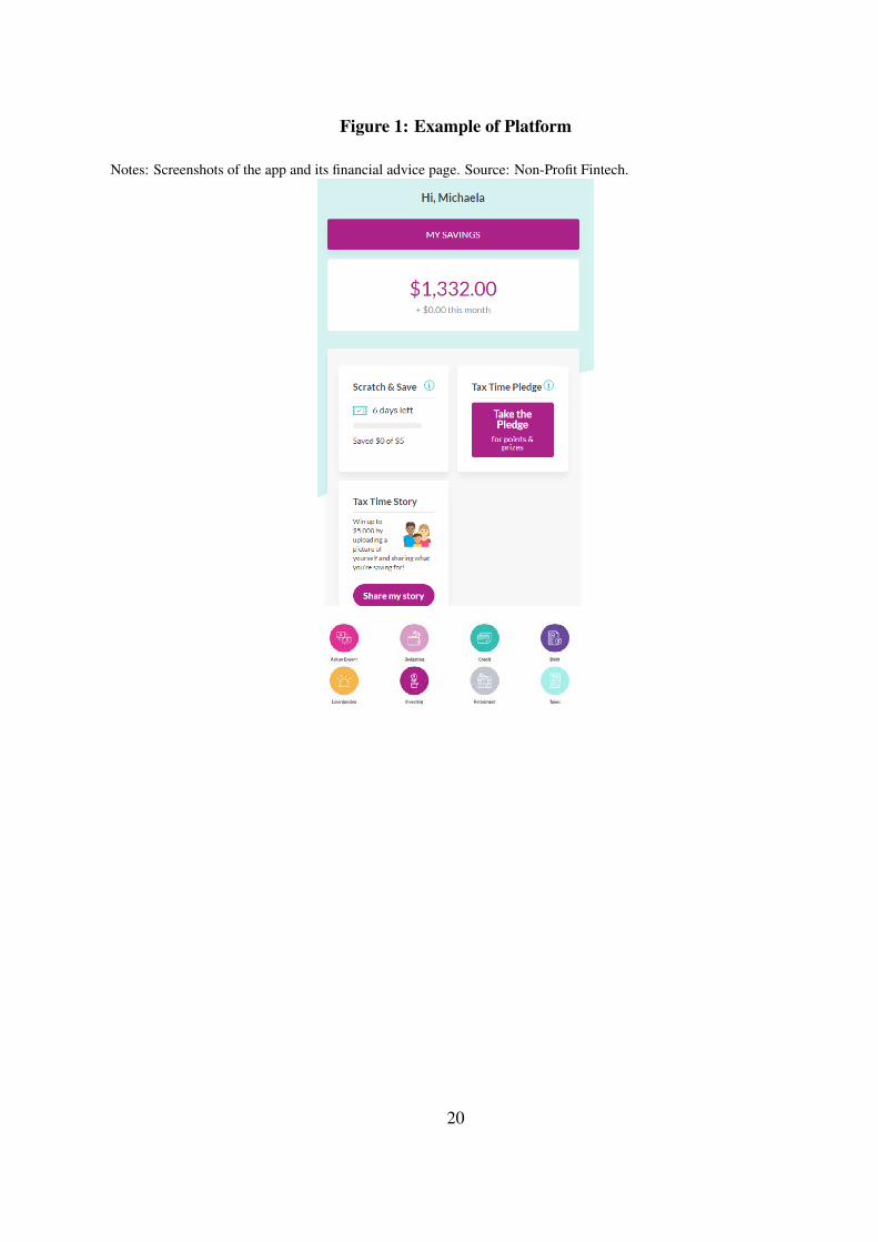
Figure 1: Example of Platform

Notes: Screenshots of the app and its financial advice page. Source: Non-Profit Fintech.

20

Figure 2: Non-Profit Fintech Users

Notes: Panel A displays the number of the non-profit Fintech users by 5-digit zip code in the US. Panel B showsthe average annual self-reported income of users by 5-digit zip code in the US (in 1,000 USD). Source: Non-ProfitFintech.

Panel A: Number of Users

Panel B: Average User Income

21

Figure 3: Household Grocery Spending Response

Notes: This graph displays how household spending changed by week in 2020. Spending is measured in daily dollars. Months are split into four periods equal in size acrossmonths. Individual fixed effects are removed prior to collapsing across individuals. Source: Non-Profit Fintech.

All Spending Grocery Spending

2040

6080

100

Mea

n Sp

endi

ng

Jan 10 2020 Feb 10 2020 Mar 10 2020

24

68

10G

roce

ries

Jan 10 2020 Feb 10 2020 Mar 10 2020

22

Figure 4: Household Spending Response Across Categories

Notes: This graph displays the response of household spending across a number of categories of spending. Spending is measured in daily dollars. Estimates are taken as thechange in household spending from the first week of February to the first week of March. Source: Non-Profit Fintech.

Retail Spending Restaurant Spending Air Travel Spending

510

1520

Ret

ail

Jan 10 2020 Feb 10 2020 Mar 10 2020

24

68

Res

taur

ants

Jan 10 2020 Feb 10 2020 Mar 10 2020

0.1

.2.3

.4Ai

r Tra

vel

Jan 10 2020 Feb 10 2020 Mar 10 2020

Food Delivery Spending Public Transit Spending Credit Card Spending

.3.4

.5.6

.7Fo

od D

eliv

ery

Jan 10 2020 Feb 10 2020 Mar 10 2020

0.0

5.1

.15

Publ

ic T

rans

it

Jan 10 2020 Feb 10 2020 Mar 10 2020

24

68

Cre

dit C

ard

Spen

ding

Jan 10 2020 Feb 10 2020 Mar 10 2020

23

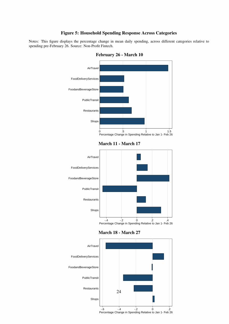
Figure 5: Household Spending Response Across Categories

Notes: This figure displays the percentage change in mean daily spending, across different categories relative tospending pre-February 26. Source: Non-Profit Fintech.

February 26 - March 10

0 .5 1 1.5Percentage Change in Spending Relative to Jan 1- Feb 26

Shops

Restaurants

PublicTransit

FoodandBeverageStore

FoodDeliveryServices

AirTravel

March 11 - March 17

-.4 -.2 0 .2 .4Percentage Change in Spending Relative to Jan 1- Feb 26

Shops

Restaurants

PublicTransit

FoodandBeverageStore

FoodDeliveryServices

AirTravel

March 18 - March 27

-.6 -.4 -.2 0 .2Percentage Change in Spending Relative to Jan 1- Feb 26

Shops

Restaurants

PublicTransit

FoodandBeverageStore

FoodDeliveryServices

AirTravel

24

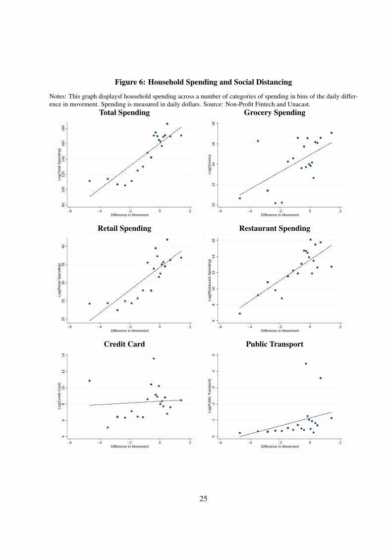
Figure 6: Household Spending and Social Distancing

Notes: This graph displaysf household spending across a number of categories of spending in bins of the daily differ-ence in movement. Spending is measured in daily dollars. Source: Non-Profit Fintech and Unacast.

Total Spending Grocery Spending

8010

012

014

016

018

0Lo

g(To

tal S

pend

ing)

-.6 -.4 -.2 0 .2Difference in Movement

1012

1416

18Lo

g(G

roce

ry-.6 -.4 -.2 0 .2

Difference in Movement

Retail Spending Restaurant Spending

2025

3035

40Lo

g(R

etai

l Spe

ndin

g)

-.6 -.4 -.2 0 .2Difference in Movement

68

1012

1416

Log(

Res

taur

ant S

pend

ing)

-.6 -.4 -.2 0 .2Difference in Movement

Credit Card Public Transport

46

810

1214

Log(

Cre

dit C

ard)

-.6 -.4 -.2 0 .2Difference in Movement

0.1

.2.3

.4.5

Log(

Publ

ic T

rans

port)

-.6 -.4 -.2 0 .2Difference in Movement

25

Figure 7: Newspaper Coverage of COVID-19, by State

Notes: This graph displays the fraction of newspaper articles in US newspapers that mentions a term related to COVID-19. Data shown for selected states. Nationwide, over3,000 newspapers are utilized.

26

Figure 8: Map of Average Partisanship, by County

Notes: This figure shows the average predicted partisan scores in US counties. Darker red shapes indicates more Republican countries, while darker blue shades indicatemore Democrat counties. Source: Gallup

(.5,.75](.25,.5](0,.25](-.25,0](-.5,-.25][-.75,-.5]

27

Figure 9: Vote Shares and Social Distancing Efforts

Notes: This figure shows a binned scatter plot of the drop in movement in all 50 US states and the District of Columbia, and the fraction of individuals who voted for DonaldTrump in the 2016 US Presidential election. Source: MIT Election Data Lab and Unacast Social Distancing Scoreboard.

0.2

.4.6

Dro

p in

Mov

emen

t

0 .2 .4 .6 .8Share of Trump 2016 Vote

28

Figure 10: Grocery Spending and Political Scores in 2020

Notes: This figure displays the response of average household daily spending for groceries. Estimates are taken as the change in household spending fromthe first week of February to the first week of March. For each category, average response is plotted for three groups: the quartile of the sample with thehighest predicted ‘democrat’ lean and the quartile of the sample with the highest predicted ‘republican’ lean and ‘independents’ who are in the middle twoquartiles. Spending is measured in daily dollars. Source: Non-Profit Fintech.

24

68

10G

roce

ries

Jan 10 2020 Feb 10 2020 Mar 10 2020

Republicans DemocratsIndependents

29

Figure 11: Household Spending Response Across Categories, by Predicted Partisanship

Notes: This figure displays the response of average household daily spending across a number of categories of spending. Estimates are taken as the change in householdspending from the first week of February to the first week of March. For each category, average response is plotted for three groups: the quartile of the sample withthe highest predicted ‘democrat’ lean and the quartile of the sample with the highest predicted ‘republican’ lean and ‘independents’ who are in the middle two quartiles.Spending is measured in daily dollars. Source: Non-Profit Fintech.

Retail Spending Restaurant Spending Air Travel Spending

510

1520

Ret

ail

Jan 10 2020 Feb 10 2020 Mar 10 2020

Republicans DemocratsIndependents

24

68

Air T

rave

l

Jan 10 2020 Feb 10 2020 Mar 10 2020

Republicans DemocratsIndependents

0.2

.4.6

.8Ai

r Tra

vel

Jan 10 2020 Feb 10 2020 Mar 10 2020

Republicans DemocratsIndependents

Food Delivery Spending Public Transit Spending Credit Card Spending

.2.4

.6.8

Food

Del

iver

y

Jan 10 2020 Feb 10 2020 Mar 10 2020

Republicans DemocratsIndependents

0.0

5.1

.15

.2.2

5Pu

blic

Tra

nsit

Jan 10 2020 Feb 10 2020 Mar 10 2020

Republicans DemocratsIndependents

24

68

10C

redi

t Car

d Sp

endi

ng

Jan 10 2020 Feb 10 2020 Mar 10 2020

Republicans DemocratsIndependents

30

Table 1: Monthly Summary Statistics

PercentilesMean Std. Dev. 10% 25% 50% 75% 90%

Number of Linked Accts 2.61 2.92 1 1 2 3 5Number of Txns 77.06 64.29 17 33 64 100 155Payroll Income $2,718.50 $3,789.80 $6.70 $410.64 $1,681.19 $3,629.03 $6,352.28Groceries $262.36 $351.75 $19.89 $48.01 $138.88 $351.75 $701.73Restaurants $318.97 $942.38 $16.32 $44.63 $124.66 $278.25 $652.35Pharmacies $53.39 $86.24 $6.47 $14.31 $30.78 $61.13 $114.26Shopping $165.15 $322.90 $8.55 $22.245 $69.995 $169.38 $371.31

Transaction-Level Obs. 691,542

Summary statistics of the final sample of active users with complete data from March 27th. Data are monthly over users’ entire smaple histories. Allstatistics are in USD.31

Table 2: Spending by Week and Heterogeneity by State

Regression of spending on indicators for the labeled time periods. Dependent variables vary across columns, with columns (1)-(3) being on a wide metric of household spendingincluding services, food and restaurants, entertainment, pharmacies, personal care and transportation. Columns (4)-(6) include only spending on restaurants, while the final set ofcolumns include spending only at grocery stores and supermarkets. ‘Shelter’ indicates that the sample is limited to users in states that, as of March 27th, had a shelter in place orderin place. ‘No Shelter’ restricts to users in states without such an order. Standard errors clustered at a user level. *p < .1, ** p < .05, *** p < .01. Source: Non-Profit Fintech.

(1) (2) (3) (4) (5) (6) (7) (8) (9)VARIABLES All Shelter No Shelter All - Rest Shelter - Rest No Shelter - Rest All - Groc Shelter - Groc No Shelter - Groc

February 26 - March 10 0.516*** 0.584*** 0.491*** 0.371*** 0.335*** 0.337*** 0.273*** 0.284*** 0.269***(0.0273) (0.0452) (0.0765) (0.0212) (0.0407) (0.0626) (0.0208) (0.0390) (0.0633)

March 11 - March 17 -0.0437 0.134** 0.0701 0.0463* 0.0523 0.159** 0.189*** 0.331*** 0.187**(0.0318) (0.0561) (0.0957) (0.0240) (0.0455) (0.0764) (0.0255) (0.0515) (0.0827)

March 18 - March 27 -0.477*** -0.245*** -0.159 -0.313*** -0.318*** -0.123 0.0745*** 0.232*** 0.0838(0.0322) (0.0558) (0.0973) (0.0235) (0.0452) (0.0784) (0.0253) (0.0519) (0.0860)

Observations 61,555 15,886 6,383 61,555 15,886 6,383 61,555 15,886 6,383R2 0.397 0.431 0.443 0.397 0.428 0.443 0.398 0.415 0.440User FE YES YES YES YES YES YES YES YES YES

32

Table 3: Spending by Week and Heterogeneity by Predicted Political Position

Regression of spending on indicators for the labeled time periods. Dependent variables vary across columns, with columns (1)-(3) being on a wide metric ofhousehold spending including services, food and restaurants, entertainment, pharmacies, personal care and transportation. Columns (4)-(6) include only spendingon restaurants, while the final set of columns include spending only at grocery stores and supermarkets. ‘Dem’ indicates that the sample is limited to users who arepredicted to be in the top quartile of most democratic leaning based on Demographic and financial indicators. ‘Rep’ indicates that the sample is limited to userswho are predicted to be in the top quartile of most Republican leaning based on demographic and financial indicators. Standard errors clustered at a user level.*p < .1, ** p < .05, *** p < .01. Source: Non-Profit Fintech.

(1) (2) (3) (4) (5) (6) (7) (8) (9)VARIABLES All Dem Rep All - Rest Dem - Rest Rep - Rest All - Groc Dem - Groc Rep - Groc

February 26 - March 10 0.516*** 0.401*** 0.505*** 0.371*** 0.292*** 0.379*** 0.273*** 0.120*** 0.298***(0.0273) (0.0524) (0.0626) (0.0212) (0.0416) (0.0480) (0.0208) (0.0393) (0.0442)

March 11 - March 17 -0.0437 -0.0642 -0.0659 0.0463* -0.0153 0.0638 0.189*** 0.176*** 0.238***(0.0318) (0.0629) (0.0729) (0.0240) (0.0491) (0.0528) (0.0255) (0.0504) (0.0562)

March 18 - March 27 -0.477*** -0.572*** -0.484*** -0.313*** -0.460*** -0.364*** 0.0745*** 0.0755 0.0595(0.0322) (0.0661) (0.0720) (0.0235) (0.0487) (0.0496) (0.0253) (0.0504) (0.0544)

Observations 61,555 15,080 12,922 61,555 15,080 12,922 61,555 15,080 12,922R2 0.397 0.388 0.386 0.397 0.392 0.381 0.398 0.397 0.393User FE YES YES YES YES YES YES YES YES YES

33

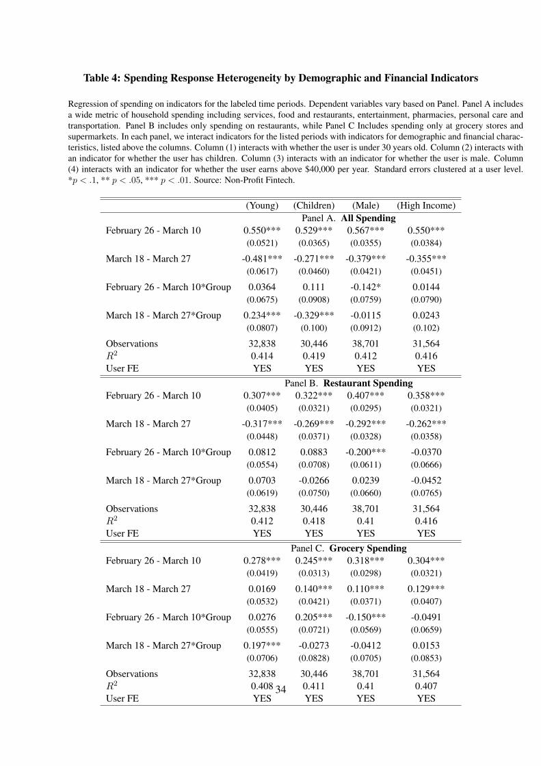
Table 4: Spending Response Heterogeneity by Demographic and Financial Indicators

Regression of spending on indicators for the labeled time periods. Dependent variables vary based on Panel. Panel A includesa wide metric of household spending including services, food and restaurants, entertainment, pharmacies, personal care andtransportation. Panel B includes only spending on restaurants, while Panel C Includes spending only at grocery stores andsupermarkets. In each panel, we interact indicators for the listed periods with indicators for demographic and financial charac-teristics, listed above the columns. Column (1) interacts with whether the user is under 30 years old. Column (2) interacts withan indicator for whether the user has children. Column (3) interacts with an indicator for whether the user is male. Column(4) interacts with an indicator for whether the user earns above $40,000 per year. Standard errors clustered at a user level.*p < .1, ** p < .05, *** p < .01. Source: Non-Profit Fintech.

(Young) (Children) (Male) (High Income)Panel A. All Spending

February 26 - March 10 0.550*** 0.529*** 0.567*** 0.550***(0.0521) (0.0365) (0.0355) (0.0384)

March 18 - March 27 -0.481*** -0.271*** -0.379*** -0.355***(0.0617) (0.0460) (0.0421) (0.0451)

February 26 - March 10*Group 0.0364 0.111 -0.142* 0.0144(0.0675) (0.0908) (0.0759) (0.0790)

March 18 - March 27*Group 0.234*** -0.329*** -0.0115 0.0243(0.0807) (0.100) (0.0912) (0.102)

Observations 32,838 30,446 38,701 31,564R2 0.414 0.419 0.412 0.416User FE YES YES YES YES

Panel B. Restaurant SpendingFebruary 26 - March 10 0.307*** 0.322*** 0.407*** 0.358***

(0.0405) (0.0321) (0.0295) (0.0321)

March 18 - March 27 -0.317*** -0.269*** -0.292*** -0.262***(0.0448) (0.0371) (0.0328) (0.0358)

February 26 - March 10*Group 0.0812 0.0883 -0.200*** -0.0370(0.0554) (0.0708) (0.0611) (0.0666)

March 18 - March 27*Group 0.0703 -0.0266 0.0239 -0.0452(0.0619) (0.0750) (0.0660) (0.0765)

Observations 32,838 30,446 38,701 31,564R2 0.412 0.418 0.41 0.416User FE YES YES YES YES

Panel C. Grocery SpendingFebruary 26 - March 10 0.278*** 0.245*** 0.318*** 0.304***

(0.0419) (0.0313) (0.0298) (0.0321)

March 18 - March 27 0.0169 0.140*** 0.110*** 0.129***(0.0532) (0.0421) (0.0371) (0.0407)

February 26 - March 10*Group 0.0276 0.205*** -0.150*** -0.0491(0.0555) (0.0721) (0.0569) (0.0659)

March 18 - March 27*Group 0.197*** -0.0273 -0.0412 0.0153(0.0706) (0.0828) (0.0705) (0.0853)

Observations 32,838 30,446 38,701 31,564R2 0.408 0.411 0.41 0.407User FE YES YES YES YES

34