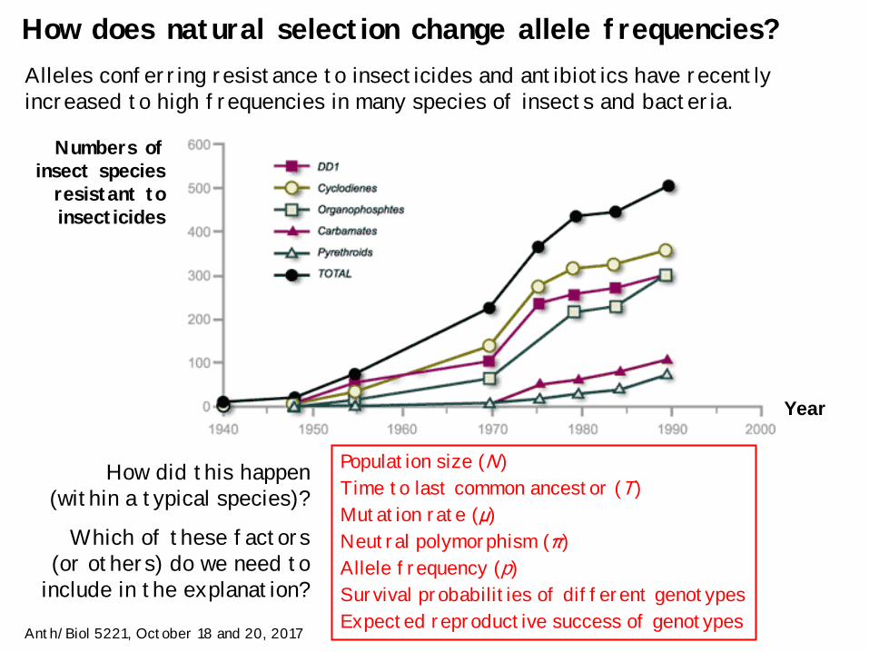
How does natural selection change allele frequencies? Alleles conferring resistance to insecticides and antibiotics have recently increased to high frequencies in many species of insects and bacteria.

Numbers of insect species

resistant to insecticides

Year

Anth/Biol 5221, October 18 and 20, 2017

How did this happen (within a typical species)?

Which of these factors (or others) do we need to

include in the explanation?

Population size (N) Time to last common ancestor (T) Mutation rate (μ) Neutral polymorphism (π) Allele frequency (p) Survival probabilities of different genotypes Expected reproductive success of genotypes

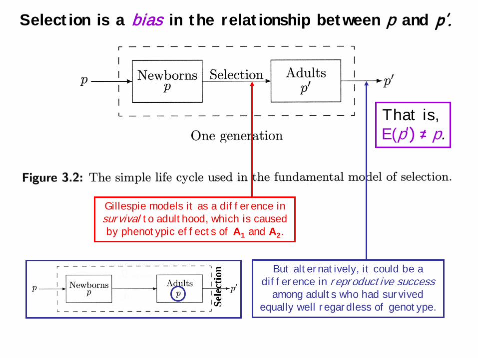
Selection is a bias in the relationship between p and p’.

Gillespie models it as a difference in survival to adulthood, which is caused by phenotypic effects of A1 and A2.

That is, E(p’) ≠ p.

But alternatively, it could be a difference in reproductive success

among adults who had survived equally well regardless of genotype. Se

lect

ion

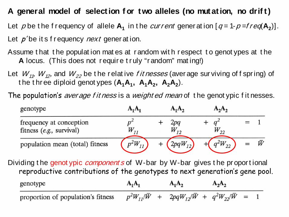
A general model of selection for two alleles (no mutation, no drift)

Let p be the frequency of allele A1 in the current generation [q = 1-p =freq(A2)].

Let p’ be its frequency next generation.

Assume that the population mates at random with respect to genotypes at the A locus. (This does not require truly “random” mating!)

Let W11, W12, and W22 be the relative fitnesses (average surviving offspring) of the three diploid genotypes (A1A1, A1A2, A2A2).

The population’s average fitness is a weighted mean of the genotypic fitnesses.

Dividing the genotypic components of W-bar by W-bar gives the proportional reproductive contributions of the genotypes to next generation’s gene pool.

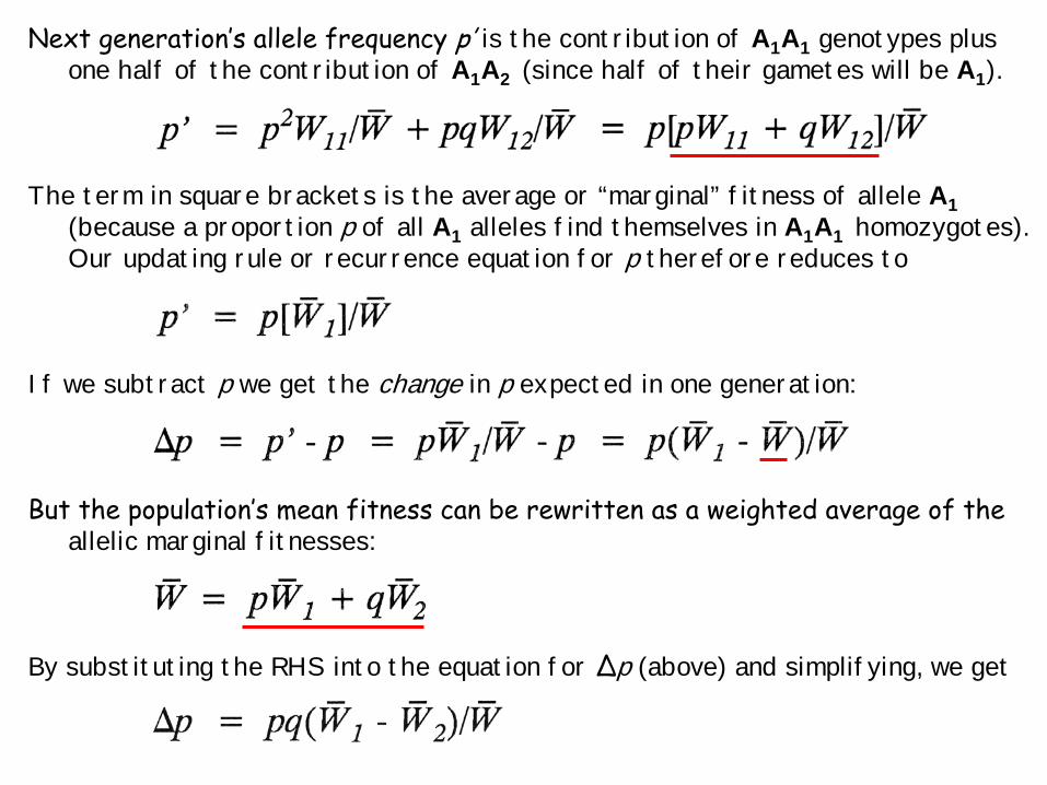
Next generation’s allele frequency p’ is the contribution of A1A1 genotypes plus one half of the contribution of A1A2 (since half of their gametes will be A1).

The term in square brackets is the average or “marginal” fitness of allele A1

(because a proportion p of all A1 alleles find themselves in A1A1 homozygotes). Our updating rule or recurrence equation for p therefore reduces to

If we subtract p we get the change in p expected in one generation: But the population’s mean fitness can be rewritten as a weighted average of the

allelic marginal fitnesses: By substituting the RHS into the equation for Δp (above) and simplifying, we get

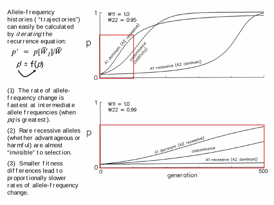
Allele-frequency histories ( “trajectories”) can easily be calculated by iterating the recurrence equation:

p’ = f(p)

(1) The rate of allele-frequency change is fastest at intermediate allele frequencies (when pq is greatest).

(2) Rare recessive alleles (whether advantageous or harmful) are almost “invisible” to selection.

(3) Smaller fitness differences lead to proportionally slower rates of allele-frequency change.

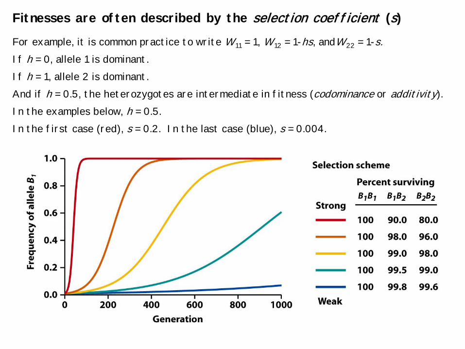
Fitnesses are often described by the selection coefficient (s) For example, it is common practice to write W11 = 1, W12 = 1-hs, andW22 = 1-s. If h = 0, allele 1 is dominant. If h = 1, allele 2 is dominant. And if h = 0.5, the heterozygotes are intermediate in fitness (codominance or additivity). In the examples below, h = 0.5. In the first case (red), s = 0.2. In the last case (blue), s = 0.004.

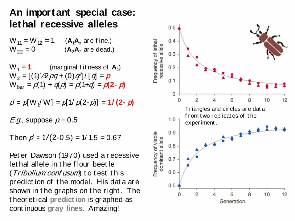
An important special case: lethal recessive alleles W11 = W12 = 1 (A1Ax are fine.) W22 = 0 (A2A2 are dead.) W1 = 1 (marginal fitness of A1) W2 = [(1)½2pq + (0)q2]/[q] = p Wbar = p(1) + q(p) = p(1+q) = p(2-p) p’ = p[W1/W] = p[1/p(2-p)] = 1/(2-p) E.g., suppose p = 0.5 Then p’ = 1/(2-0.5) = 1/1.5 = 0.67 Peter Dawson (1970) used a recessive lethal allele in the flour beetle (Tribolium confusum) to test this prediction of the model. His data are shown in the graphs on the right. The theoretical prediction is graphed as continuous gray lines. Amazing!

Triangles and circles are data from two replicates of the experiment.

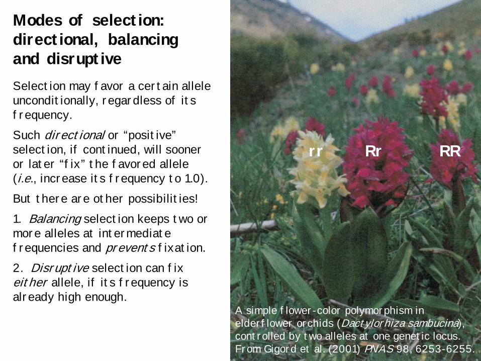
Modes of selection: directional, balancing and disruptive

RR Rr rr

A simple flower-color polymorphism in elderflower orchids (Dactylorhiza sambucina), controlled by two alleles at one genetic locus. From Gigord et al. (2001) PNAS 98, 6253-6255.

Selection may favor a certain allele unconditionally, regardless of its frequency. Such directional or “positive” selection, if continued, will sooner or later “fix” the favored allele (i.e., increase its frequency to 1.0). But there are other possibilities! 1. Balancing selection keeps two or more alleles at intermediate frequencies and prevents fixation. 2. Disruptive selection can fix either allele, if its frequency is already high enough.

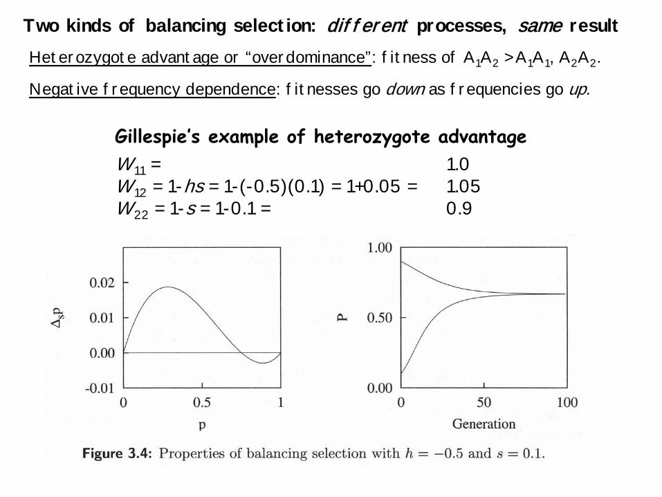
Two kinds of balancing selection: different processes, same result Heterozygote advantage or “overdominance”: fitness of A1A2 > A1A1, A2A2.

Negative frequency dependence: fitnesses go down as frequencies go up.

Gillespie’s example of heterozygote advantage W11 = 1.0 W12 = 1-hs = 1-(-0.5)(0.1) = 1+0.05 = 1.05 W22 = 1-s = 1-0.1 = 0.9

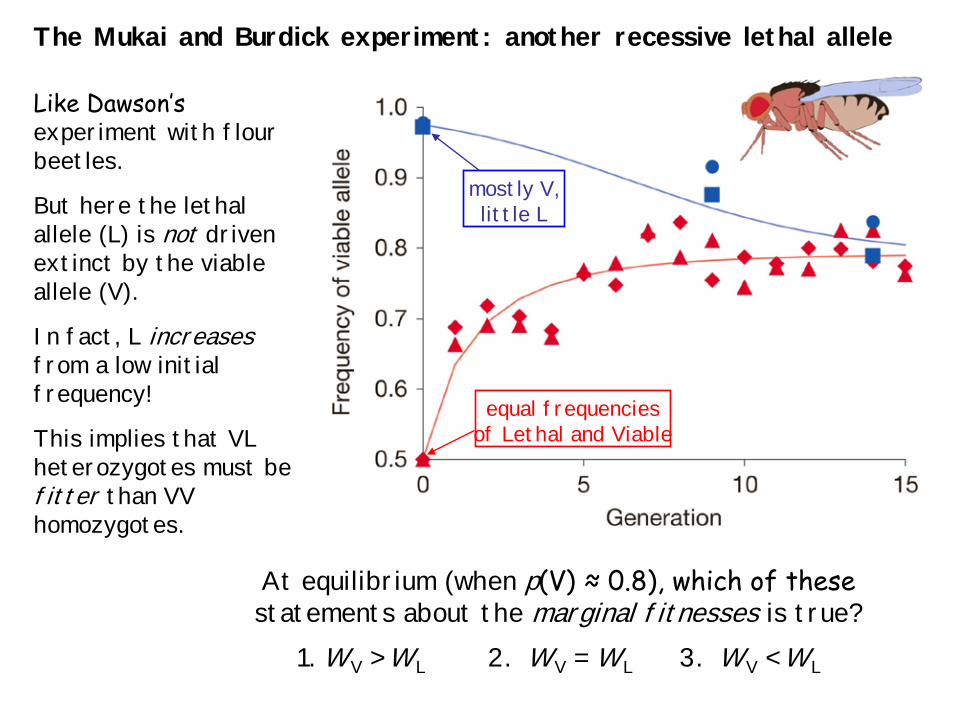
The Mukai and Burdick experiment: another recessive lethal allele

Like Dawson’s experiment with flour beetles.

But here the lethal allele (L) is not driven extinct by the viable allele (V).

In fact, L increases from a low initial frequency!

This implies that VL heterozygotes must be fitter than VV homozygotes.

At equilibrium (when p(V) ≈ 0.8), which of these statements about the marginal fitnesses is true?

1. WV > WL 2. WV = WL 3. WV < WL

mostly V, little L

equal frequencies of Lethal and Viable

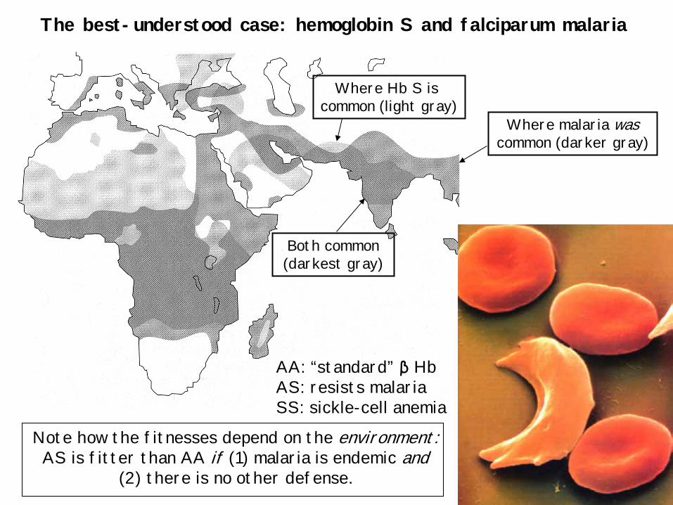
The best-understood case: hemoglobin S and falciparum malaria

Where Hb S is common (light gray)

Where malaria was common (darker gray)

Both common (darkest gray)

AA: “standard” β Hb AS: resists malaria SS: sickle-cell anemia

Note how the fitnesses depend on the environment: AS is fitter than AA if (1) malaria is endemic and

(2) there is no other defense.

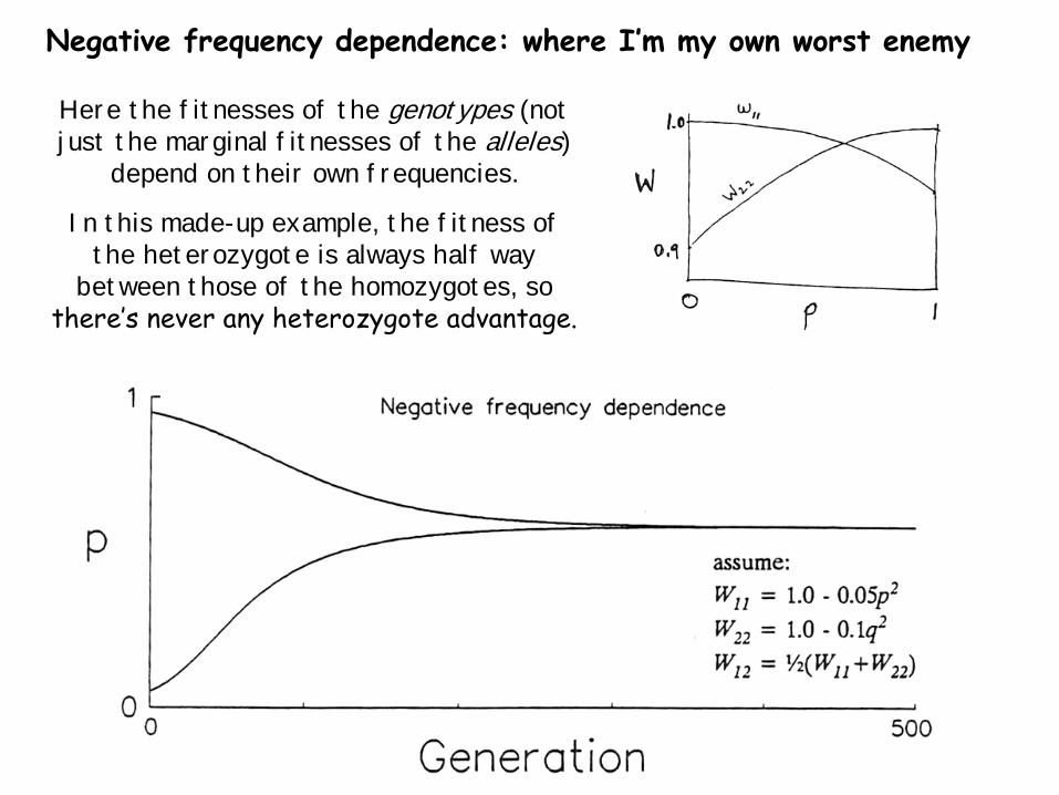
Negative frequency dependence: where I’m my own worst enemy

Here the fitnesses of the genotypes (not just the marginal fitnesses of the alleles)

depend on their own frequencies.

In this made-up example, the fitness of the heterozygote is always half way

between those of the homozygotes, so there’s never any heterozygote advantage.

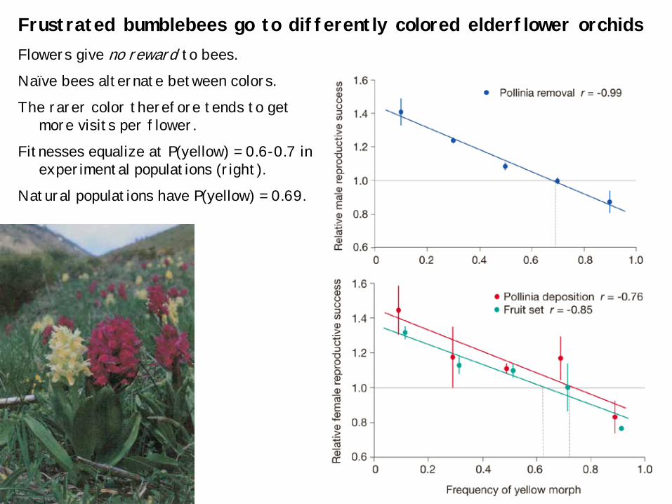
Frustrated bumblebees go to differently colored elderflower orchids Flowers give no reward to bees. Naïve bees alternate between colors. The rarer color therefore tends to get

more visits per flower. Fitnesses equalize at P(yellow) = 0.6-0.7 in

experimental populations (right). Natural populations have P(yellow) = 0.69.

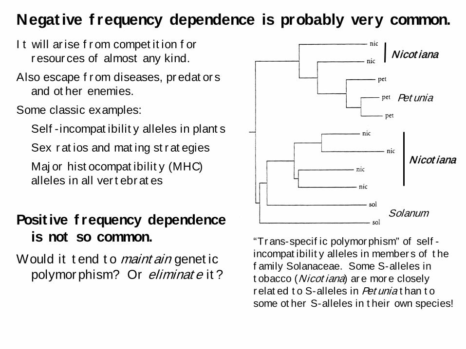
Negative frequency dependence is probably very common. It will arise from competition for

resources of almost any kind. Also escape from diseases, predators

and other enemies. Some classic examples: Self-incompatibility alleles in plants Sex ratios and mating strategies Major histocompatibility (MHC)

alleles in all vertebrates

Positive frequency dependence is not so common.

Would it tend to maintain genetic polymorphism? Or eliminate it?

Nicotiana

Nicotiana

Petunia

Solanum

“Trans-specific polymorphism” of self-incompatibility alleles in members of the family Solanaceae. Some S-alleles in tobacco (Nicotiana) are more closely related to S-alleles in Petunia than to some other S-alleles in their own species!

How and when do typical genes contribute to fitness? A major puzzle: Most genes appear to be unnecessary! Half or more can be “knocked out” (fully disabled) in yeast, worms, flies and

even mice, without any obvious phenotypic effects (in the lab, anyway). But these genes are maintained in evolution, so they must be useful. How? Two hypotheses: (1) Most are “special-purpose” genes needed only under certain circumstances

(stresses that occur in nature but not in the lab). (2) Most are “fine-tuning” genes that increase the efficiency or accuracy of

some physiological or developmental process in most environments.

Experimental test devised by Joe Dickinson: Compete “no-phenotype knockouts” against genotypes that are identical except for the knockout, and let natural selection measure their relative fitnesses. Dickinson talked Janet Shaw (a yeast cell biologist) and John Thatcher (an undergraduate) into helping him try to do this with yeast.

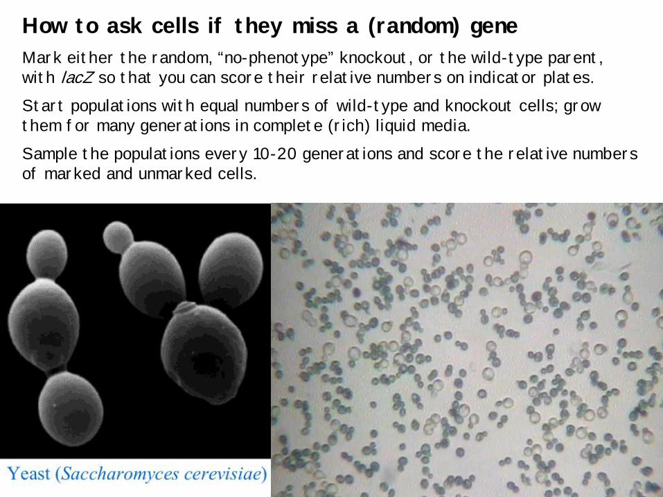
How to ask cells if they miss a (random) gene Mark either the random, “no-phenotype” knockout, or the wild-type parent, with lacZ so that you can score their relative numbers on indicator plates. Start populations with equal numbers of wild-type and knockout cells; grow them for many generations in complete (rich) liquid media. Sample the populations every 10-20 generations and score the relative numbers of marked and unmarked cells.

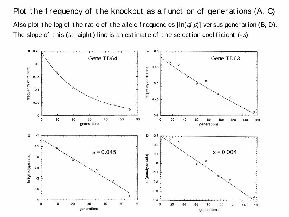
Plot the frequency of the knockout as a function of generations (A, C) Also plot the log of the ratio of the allele frequencies [ln(q/p)] versus generation (B, D). The slope of this (straight) line is an estimate of the selection coefficient (-s).

s = 0.045 s = 0.004

Gene TD64 Gene TD63

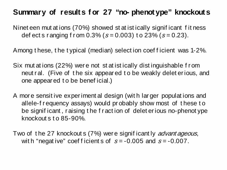
Summary of results for 27 “no-phenotype” knockouts

Nineteen mutations (70%) showed statistically significant fitness defects ranging from 0.3% (s = 0.003) to 23% (s = 0.23).

Among these, the typical (median) selection coefficient was 1-2%. Six mutations (22%) were not statistically distinguishable from

neutral. (Five of the six appeared to be weakly deleterious, and one appeared to be beneficial.)

A more sensitive experimental design (with larger populations and

allele-frequency assays) would probably show most of these to be significant, raising the fraction of deleterious no-phenotype knockouts to 85-90%.

Two of the 27 knockouts (7%) were significantly advantageous,

with “negative” coefficients of s = -0.005 and s = -0.007.

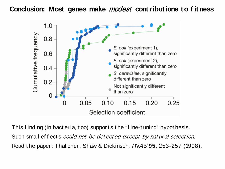
Conclusion: Most genes make modest contributions to fitness

This finding (in bacteria, too) supports the “fine-tuning” hypothesis. Such small effects could not be detected except by natural selection. Read the paper: Thatcher, Shaw & Dickinson, PNAS 95, 253-257 (1998).

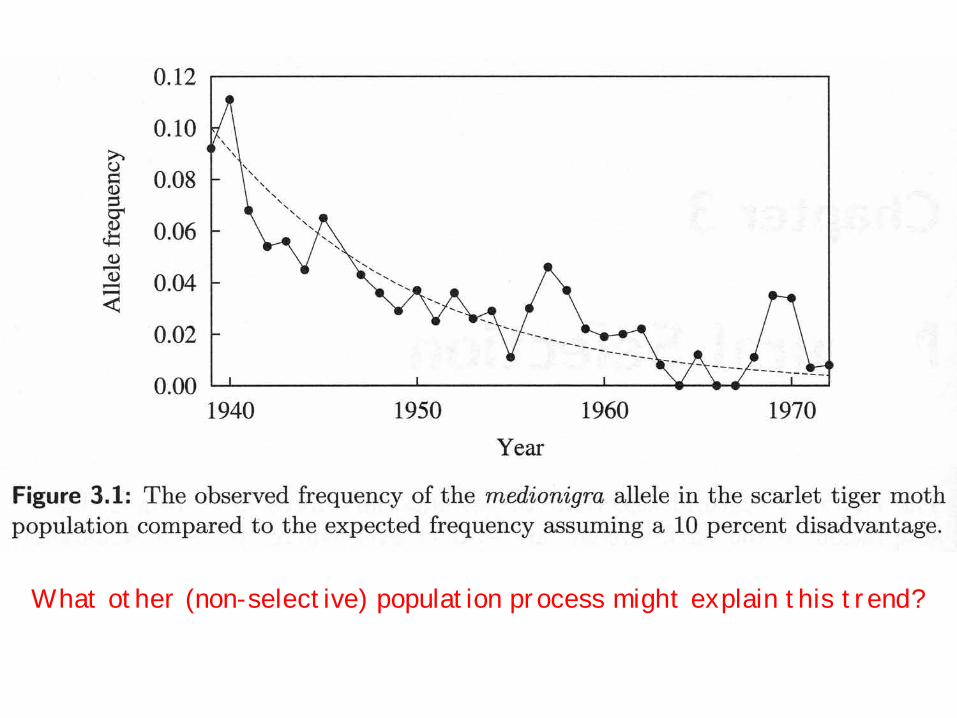
What other (non-selective) population process might explain this trend?

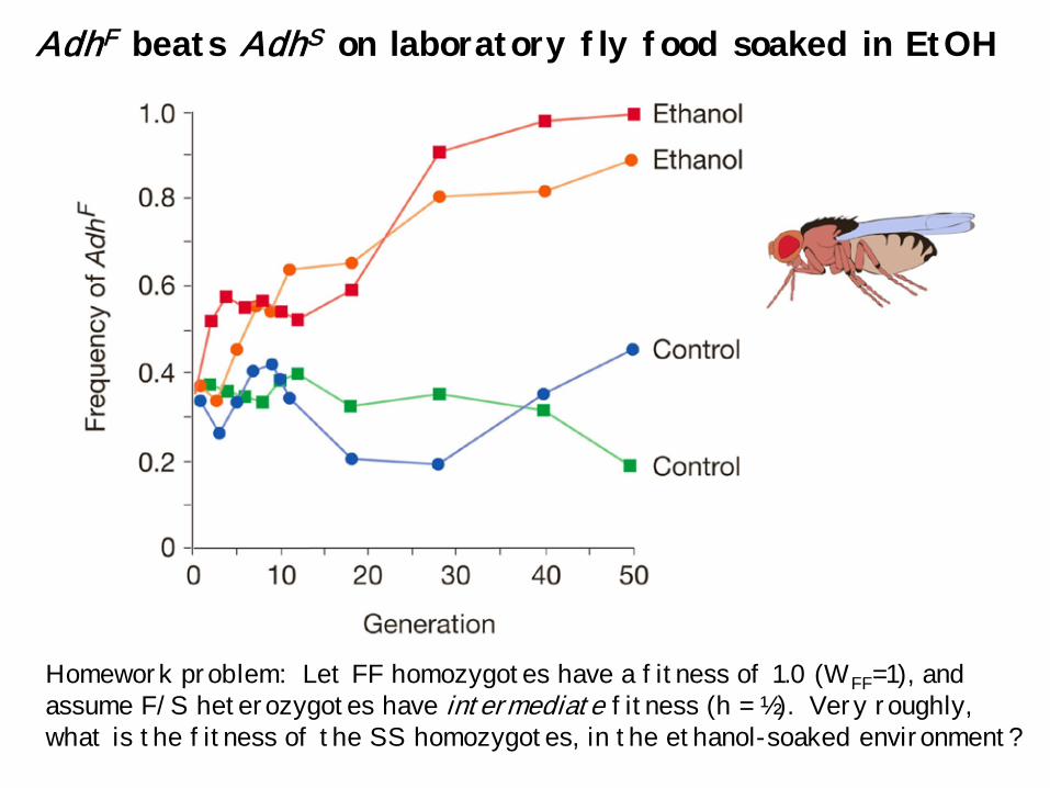
AdhF beats AdhS on laboratory fly food soaked in EtOH

Homework problem: Let FF homozygotes have a fitness of 1.0 (WFF=1), and assume F/S heterozygotes have intermediate fitness (h = ½). Very roughly, what is the fitness of the SS homozygotes, in the ethanol-soaked environment?