how does reach‐scale stream‐hyporheic transport vary with...

RESEARCH ARTICLE10.1002/2016WR018832

How does reach-scale stream-hyporheic transport vary withdischarge? Insights from rSAS analysis of sequential tracerinjections in a headwater mountain streamC. J. Harman1, A. S. Ward2, and A. Ball1

1Department of Geography and Environmental Engineering, Johns Hopkins University, Baltimore, Maryland, USA, 2Schoolof Public and Environmental Affairs, Indiana University, Bloomington, Indiana, USA

Abstract The models of stream reach hyporheic exchange that are typically used to interpret tracer dataassume steady-flow conditions and impose further assumptions about transport processes on the interpre-tation of the data. Here we show how rank Storage Selection (rSAS) functions can be used to extract‘‘process-agnostic’’ information from tracer breakthrough curves about the time-varying turnover of reachstorage. A sequence of seven slug injections was introduced to a small stream at base flow over the courseof a diel fluctuation in stream discharge, providing breakthrough curves at discharges ranging from 0.7 to1.2 L/s. Shifted gamma distributions, each with three parameters varying stepwise in time, were used tomodel the rSAS function and calibrated to reproduce each breakthrough curve with Nash-Sutcliffe efficien-cies in excess of 0.99. Variations in the fitted parameters over time suggested that storage within the reachdoes not uniformly increase its turnover rate when discharge increases. Rather, changes in transit time aredriven by both changes in the average rate of turnover (external variability) and changes in the relative ratethat younger and older water contribute to discharge (internal variability). Specifically, at higher discharge,the turnover rate increased for the youngest part of the storage (corresponding to approximately 5 times thevolume of the channel), while discharge from the older part of the storage remained steady, or declinedslightly. The method is shown to be extensible as a new approach to modeling reach-scale solute transportthat accounts for the time-varying, discharge-dependent turnover of reach storage.

1. Introduction

Hyporheic exchange is known to be mechanistically coupled to the hydrological controls of stream dis-charge and near-stream hydraulic gradients. However, the most common method used to characterizehyporheic exchange—the analysis of solute tracer breakthrough curves—has failed to identify consistentcontrols on hyporheic exchange under time-variable hydrologic conditions [e.g., Ward et al., 2013a; Paynet al., 2009]. To-date, time-variable hyporheic exchange has been reported in response to variable base flowconditions [Ward et al., 2012; Payn et al., 2009; Ward et al., 2013b], diel fluctuations in discharge [Loheide andLundquist, 2009; Sawyer and Cardenas, 2009; Sawyer et al., 2013; Wondzell et al., 2009a], and storm eventresponses [Ward et al., 2013a; Malzone and Lowry, 2014; Schmadel et al., 2016]. Several studies that includehigh replication in space or through storm events report that observed variations in reach-scale tracer trans-port and inferred hyporheic exchange could not be explained by discharge alone [Wondzell, 2006; Wardet al., 2012; Payn et al., 2009; Ward et al., 2013b]. As such, it remains unknown if observed variations in hypo-rheic exchange and reach-scale transport arise because of variations in stream discharge, changes in hypo-rheic flow paths themselves, or a combination of the two.

This confusion may be, in part, a result of limitations in the methods used to interpret solute tracer stud-ies—in particular, their ability to account for transient hydrological dynamics. Recent work has demonstrat-ed that transport variability in response to dynamic hydrologic forcing can be decomposed into twodistinct components, termed external and internal variability [Kim et al., 2016]. Both types might contributeto overall transport variability of a given system, though one may dominate over the other. Neither is wellrepresented in most of the methods used to interpret tracer breakthrough curves.

A more detailed discussion of these concepts is provided in Kim et al. [2016], but they can be understoodintuitively for the case were a hydrodynamic system can be reduced to a set of streamtubes, or more loosely

Key Points:� Seven tracer injections over 28 h

analyzed using rank StorageSelection function theory of time-varying transit time distributions� rSAS results show fluctuations in

turnover rate of reach storage at baseflow limited to a volume 5 timeslarger than visible channel� Method suggests an approach to

parsimonious reach-scale solutetransport that accounts for time-varying stream-hyporheic exchangedynamics

Correspondence to:C. J. Harman,[email protected]

Citation:Harman, C. J., A. S. Ward, and A. Ball(2016), How does reach-scale stream-hyporheic transport vary withdischarge? Insights from rSAS analysisof sequential tracer injections in aheadwater mountain stream, WaterResour. Res., 52, doi:10.1002/2016WR018832.

Received 25 FEB 2016

Accepted 2 AUG 2016

Accepted article online 5 AUG 2016

VC 2016. American Geophysical Union.

All Rights Reserved.

HARMAN ET AL. TIME-VARIABLE STREAM TRANSPORT 1

Water Resources Research

PUBLICATIONS

http://dx.doi.org/10.1002/2016WR018832

http://onlinelibrary.wiley.com/journal/10.1002/(ISSN)1944-7973/

http://publications.agu.org/

as a set of flow pathways. External variability refers to changes in the overall flow rate through set of allflow pathways, without implying any change in the proportion of flow through one flow pathway relativeto another. If all variability is external, the velocity along all flow paths increases proportionally to accommo-date an increase in flow. The ratio of the flux rate along any two flow paths remains constant. Internal vari-ability implies that the flow through some parts of the system increases (or decreases) by a differentproportion than through other parts. The velocity field has changed in some way other than a proportionalscaling. This reorganization of relative flow magnitudes may arise from a fluctuation in the potentiometricfield around a stream or changing interactions between streams and their catchments [Harvey and Bencala,1993; Ward et al., 2016]. However, in most hydrologic systems (with the possible exception of a confinedaquifer), a change in flow through the system will induce both internal and external variability. If we canquantify these two contributions, we can ask: what are the relative contributions of each? and what doesthe structure of the internal variability tell us about the changing structure of the flow paths?

Common methods for analyzing tracer data and modeling stream reaches typically assume steady flow,and even those that allow for variable flow in-channel assume steady flow through the transient storagezones. In all cases, models are subject to two primary limitations. First, models are based on conceptual rep-resentations of the real system and necessarily reduce complexity. The most common approaches [Bencalaand Walters, 1983; Haggerty et al., 2000; Worman et al., 2002] use inverse modeling to fit experimentalresults, analyzing the best fit parameter set to represent the dominant processes in the stream-hyporheicsystem. While adding processes may improve fit [Briggs et al., 2009; Kerr et al., 2013; Choi et al., 2000], theaddition of processes and parameters increases the field observations required to parameterize the modeland may increase existing problems with parameter interaction and/or uncertainty [Wagner and Harvey,1997; Kelleher et al., 2013]. Second, stream transport models commonly require a static and spatially homo-geneous transit time distribution for storage locations. Steady flow is assumed, implicitly or explicitly, when-ever tracer breakthrough curves are interpreted in terms of a fixed transit time distribution. Runkel et al.[1998] coupled an unsteady flow model with the transient storage model, dynamically adjusting streamarea and advection with discharge but fixing other parameters describing exchange between the streamand hyporheic zone. Still, this approach remains uncommon and experimentalists may lack data to describethe time-variable parameter relationships. Other techniques such as the concept of ‘‘flow-weighted time’’may be applied [e.g., Rodhe et al., 1996], but have not been broadly attempted in studies of stream-hyporheic exchange.

Overall, existing methods fail to address the deeper ‘‘process’’ issue: the flow paths themselves are likely tochange in response to changes in discharge—i.e., changes in discharge will induce external and internalvariability. As such, the transit time distribution will be time-varying even in flow-weighted time [Kim et al.,2016]. This limitation cannot be addressed by simply allowing the shape of the assumed transit time distri-butions to change in time, as this will lead to mass balance errors [Botter et al., 2010; Harman, 2015]. It istherefore important to better understand how internal variability is linked to stream discharge. Discharge iscommonly viewed a master variable in stream corridors, linked to predictable patterns in ecosystem func-tion [Vannote et al., 1980; Stanford and Ward, 1993], geomorphology [Leopold and Maddock, 1953], and sol-ute transport [Gooseff et al., 2008; Fischer et al., 1979]. However, the internal variability of hyporheic zoneshas received limited study, because subsurface observations are difficult to make in the field [Bencala et al.,2011]. Still, several recent studies demonstrate apparent internal variability in hyporheic zones, observingapparent flow path-scale responses to hydrologic dynamics [Voltz et al., 2013; Dudley-Southern and Binley,2015].

The concept of a rank Storage Selection (or rSAS) function provides an alternative approach to break-through curve analysis that separates the influence of internal and external variability, allowing their relativeinfluence on transport to be examined. This approach was developed and applied initially for catchment-scale applications [Harman, 2015] and has not yet been applied to reach-scale studies of stream-hyporheicsystems. The rSAS theory is a generalization of the theory of transit time distributions to fully time-variableconditions. The transit time distribution is not fit to the breakthrough curve directly [e.g., Kirchner et al.,2000]. Instead, a pdf is selected for the rSAS function, and this is combined with the time-varying flow toyield a time-varying transit time distribution. The parameters of the rSAS function can be chosen to bestreproduce the observed data. Unlike the transit time distribution, the rSAS function only varies in timewhen there is internal variability.

Water Resources Research 10.1002/2016WR018832


The objective of this study is to examine time-variable transport in a stream-hyporheic system in the con-text of internal and external variability. We take the well-studied Watershed 1 (WS01) at the H.J. AndrewsExperimental Forest as a test-case to assess the relative roles of internal and external variability in explainingstream-hyporheic observations. Using existing studies, it is possible to formulate (apparently) contradictoryhypotheses that emphasize the role of either internal or external variability:

H1: Internal variability is the dominant control on stream-hyporheic exchange. Stream solute tracer studies inWS01 demonstrate time-variable transport at the reach scale through base flow recession and storm events[Wondzell et al., 2007, 2009a; Ward et al., 2013a]. Based on in-stream tracer observations, past efforts con-clude that discharge alone (i.e., external variability) is not sufficient to explain in-stream solute tracer obser-vations [Ward et al., 2013a]. As such, internal variability has been invoked as a possible explanatorymechanism [Ward et al., 2013a]. Indeed, Voltz et al. [2013] report time-variable hydraulic gradients in the val-ley bottom, a likely indicator of spatial reorganization of hyporheic flow paths (i.e., internal variability). Fur-thermore, Ward et al. [2016] found time-variable hyporheic transport through base flow recession atmonitoring wells distal from the stream itself. Because conceptual models have invoked internal variabilityto explain observations [Ward et al., 2013a,], and because internal variability has been observed [Voltz et al.,2013; Ward et al., 2016], internal variability can be hypothesized to be the dominant control on stream-hyporheic exchange in WS01.

H2: External variability is the dominant control on stream-hyporheic exchange. More recently, Ward et al.[2016] analyzed direct subsurface observations to assess internal variability through base flow recession.They found that the behavior of flow paths near the stream is dominated by hydrostatic gradients aroundpool-riffle-step structures, and was minimally variable through base flow recession (i.e., no internal variabili-ty for these flow paths); only more distal flow paths exhibited variation in their time scales. Because streamsolute tracers are known to be primarily sensitive to the shortest and fastest hyporheic flow paths (com-monly the ‘‘window of detection,’’ in the sense of Harvey et al. [1996]), and because these shortest and fast-est flow paths were observed to be time-invariant [Ward et al., 2016], external variability can behypothesized to be the dominant control on stream-hyporheic exchange in WS01.

To test these hypotheses, we conducted a series of solute tracer injections during a period of changingstreamflow conditions in WS01. By applying the rSAS approach to the experimental data set, we estimatethe relative role of internal and external variability in yielding the observed transport in the stream. Further-more, this approach allows us to relate changes in hydrologic forcing to changes in the Storage Selectionfunction, suggesting an approach to forward modeling of stream reach transport.

2. Background

2.1. Rank Storage Selection (rSAS) TheoryStorage Selection (SAS) theory provides a basis for interpreting tracer data and modeling solute transportthrough arbitrary control volumes [Rinaldo et al., 2015; Harman, 2015]. The concept of a rank Storage Selec-tion (rSAS) function was presented in Harman [2015], and extends previous approaches [van der Velde et al.,2012]. An outline of the theory is provided here, with additional developments tailored to the needs of thepresent work, but full details can be found in the cited papers.

rSAS theory is based on a formal accounting of the ‘‘age’’ of infinitesimal parcels of water in a control vol-ume. The control volume can be of any size, but the fluxes of water across its boundary must be known.(Note that fluxes of water here are calculated in terms of volume, rather than mass, since we assume com-pressibility is negligible.) Here the control volume will be the stream reach, including its hyporheic and in-channel transient storage zone. We assume that down-valley transport in the hyporheic zone across thereach boundaries is negligible (as many commonly used models do, such as the transient storage model ofBencala and Walters [1983]), and that gross inflows and outflows of groundwater are negligible over thestudy reach (note the possible effects of riparian potential gradients on the structure of the rSAS functionwill be examined). The rSAS framework could be extended to account for groundwater transport if addition-al hydrogeologic data were available to quantify these fluxes. The age T of a parcel of water at time t isdefined relative to the time ti that it entered the system with the inflow: T 5 t 2 ti. Following the definitionsused in previous papers [Harman, 2015; Rinaldo et al., 2015], PS(T,t) is the distribution of ages of all water instorage at time t (or pS(T,t) when referring to the probability density function, or pdf). The transit time of a



parcel is the age T of the parcel at the time that it exits as discharge at the downstream end of the reach.The backward transit time distribution PQ(T,t) (or pQ(T,t) for the pdf) is the probability distribution represent-ing the transit times T of all the parcels exiting at a particular time t.

In rSAS theory, a new variable is introduced, the age-ranked storage ST (which has units of volume [L3] or vol-ume normalized by area [L]), representing the volume of water in the control volume with an age less thanT at time t. This is simply an unnormalized version of the cumulative distribution of ages in storage (i.e., iftotal storage S were known, we could calculate PSðT ; tÞ5ST ðT ; tÞ=SðtÞ). The value of ST(T,t) associated with acertain age T is the volume of water that has entered after time t 2 T, and remains in the system at time t. Itcan therefore be interpreted as a measure of the progress through storage of the water that entered attime t 2 T. If ST(T,t) is close to zero, the T-aged water is amongst the youngest in the system. If ST(T,t) is closeto the total storage S(t), it is amongst the oldest.

We can also define a similar variable QT(T,t) (units of [L3 T21] or [L T21]) representing the rate water with anage less than T is leaving the system at time t. This, in turn is simply an unnormalized version of the transittime distribution, so that PQðT ; tÞ5QT ðT ; tÞ=QðtÞ.

The age-ranked storage ST can be determined from a conservation of mass law for water less than an age T.This is given by:

ddt

ST ðt2ti ; tÞ5 @ST

@T1@ST

@t5JðtÞ2QT ðT ; tÞ (1)

The left-hand side of this equation gives the rate of change of the amount of water younger than a certainage T. This is the volume of water that entered the system since time t 2 T remaining in the system at timet. The right-hand side accounts for controls on this. First, new water flowing into the control volume J(t)(which has units of [L3 T21] or [L T21]) has age zero, so this adds to ST. Second, QT(T,t) is the rate this water isbeing removed from the control volume.

Since the function ST(T,t) maps ages T onto volumes ST in a monotonically increasing way, it is possible toexpress the same probability that PQ(T,t) gives in terms of T, in terms of ST instead. That is, we can constructa function XQðST ; tÞ such that XQðST ; tÞ5PQðT ; tÞ when ST 5ST ðT ; tÞ. The resulting cumulative distributionfunction, XQðST ; tÞ, is called the rank Storage Selection (rSAS) function for the discharge. The rSAS functionis a probability distribution defined over the total storage in the system. Taking the derivative of the abovedefinition, we find that pQðT ; tÞ5xQðST ; tÞ@ST=@T , where xQðST ; tÞ is the probability density function (pdf)of the rSAS function. That is:

pQðT ; tÞ@T5xQðST ; tÞ@ST (2)

for ST 5ST ðT ; tÞ. In other words, the fraction of discharge derived from age increment @T is equal to the frac-tion from age-ranked storage increment @ST . That is, xQðST ; tÞ is simply the transit time distributionexpressed in terms of storage, rather than age. If the fluxes (Q(t) and J(t)) and rSAS function XQðST ; tÞ areknown for all t, the conservation law can be solved to provide the mapping ST 5ST ðT ; tÞ that allows thetime-varying transit time distribution pQ(T,t) to be recovered.

Finally, if the inflow contains a concentration CJ(t) of an ideal conservative tracer, the outflow concentrationCQ(t) is determined by the integral [Rinaldo et al., 2011]:

CQðtÞ5ðt

21CJðtiÞpQðt2ti; tÞdti (3)

This integral reduces to a simple convolution for the case of time-invariant pQ.

2.2. Internal and External VariabilityThe rSAS function can itself be a time-varying distribution, allowing us to account for changes in the internaltransport dynamics of the system, in addition to rigorously accounting for external variability due to thetime-variable inflows and outflows. We can examine the nature of internal and external variability revealedby the stream breakthrough curve data by recasting the framework described above in two different ways.First, by taking the derivative of ST(T,t) with respect to T, we obtain the age-rank storage density sT(T,t),



which refers to the (infinitesimal) volume of water that entered at time t 2 T that is still in the system attime t. Once this volume enters it is depleted by the outflows at a rate given by qT ðT ; tÞ5@QT=@T . Thus:

ddt

sT ðt2ti; tÞ5 @sT

@T1@sT

@t52qT ðT ; tÞ (4)

which is simply the derivative of equation (1) with respect to age T.

From the definition PQðT ; tÞ5XQðST ; tÞ, it follows that qT ðT ; tÞ5QðtÞxQðST ; tÞsT ðT ; tÞ. This shows that therate that water of age T is discharged from the system depends on (1) the overall rate of discharge, (2) thelocation of that water in the overall age-ranked storage ST 5ST ðT ; tÞ, and (3) the value of the rSAS functionxQðST ; tÞ at that rank in storage at that time.

In the absence of internal variability, the rSAS function is constant in time [Kim et al., 2016], so thatxðST ; tÞ5xðST Þ. Then qT(T,t) reduces to QðtÞxQðST ÞsT ðT ; tÞ. Note that the age-ranked storage density sT(T,t)is still time-variable because the discharge Q(t) is, and hence pQ(T,t) varies in time. However, water of agerank ST always represents the same proportion of the total discharge. Thus, when the rSAS function is fixedin time, all transport variability is external variability, and there is no internal variability.

Conversely, we could fix the flux at a constant rate J(t) 5 Q(t) 5 Q0, while allowing the rSAS function to vary,so that the rate is then qT ðT ; tÞ5Q0 xðST ; tÞsT ðT ; tÞ. Then all variability is internal with no external variability.Finally, if flow was steady and the rSAS function was fixed, transport would lack either form of variability,and the rate would be a function only of the location of the parcel in age-ranked storageqT ðTÞ5Q0xðST ÞsT ðTÞ. In that case, sT (and ST) would vary only with age and not with time, and the conserva-tion law (equation (1)) reduces to:

dsT

dT52Q0 xQðST ðTÞÞÞ (5)

This implies that the transit time distribution is also fixed in time. The equivalent fixed transit time distribu-tion can be found using the definition PQðTÞ5XðST Þ, and integrating the conservation equation to obtainthe (fixed) value of ST corresponding to each age T [Harman, 2015].

These cases are summarized as follows:

qT 5 QðtÞ3 xðST ; tÞ3 sT ðT ; tÞ internal and external variability

QðtÞ3 xðST Þ3 sT ðT ; tÞ external variability only

Q0 3 xðST ; tÞ3 sT ðT ; tÞ internal variability only

Q0 3 xðST Þ3sT ðTÞ no variability

In this study, we will assess how the rSAS approach is able to reproduce observed stream tracer dynamicswhen different combinations of internal and external variability are assumed.

2.3. Dynamics of Storage TurnoverA second way to reformulate this framework can provide further insight into the behavior of storage withdifferent ages. Given an age T, we can (conceptually) divide the water in storage into a part that is youngerthan T, which is ST(T,t), and a part that is older than T, which we will call ST ðT ; tÞ. Note that the sum of theseis the total storage:

ST ðT ; tÞ1ST ðT ; tÞ5SðtÞ (6)

We do not know the total storage of the stream reach, but can estimate the changes in storage relative tosome reference state Sref (which may be the initial condition) from conservation of mass. DefiningDSðtÞ5SðtÞ2Sref and DST ðT ; tÞ5ST ðT ; tÞ2Sref , we can see that:

DST ðT ; tÞ5DSðtÞ2ST ðT ; tÞ (7)

There is an advantage to considering the age-ranked fluxes in terms of DST rather than ST in time-variableconditions. Much of the time-variability in hydrologic systems is associated with young water, while theolder water moves at a steadier pace [Harman, 2015]. Thus, there ought to be a way to quantify the rate



that ‘‘old’’ water is being discharged from the ‘‘old’’ parts of storage. Defining the flux of old water from thesystem as the complement to the flux of young water, QT 5Q2QT , we can define a function that describesthe rate that old water is being discharged from storage:

QT 5FSðDST ; tÞ5QðtÞð12XQðDS2DST ; tÞÞ (8)

or alternatively in a density form, to isolate just the flux rate of water along a flow path representing a par-ticular age rank in storage:

@QT

@ST5fSðDST ; tÞ5QðtÞxQðDS2DST ; tÞÞ (9)

where fS5@FS=@DST .

The advantage of considering variations in QT (rather than just variations in X) is that through it we canunderstand in an intuitive way how a fluctuation in Q affects the shape of the rSAS function. Consider ahydrologic system in which an increase in total flow through the system (and consequent increase in totalstorage) is largely accommodated by a higher rate of turnover of the youngest water in the system, whilethe older water continues to turnover at the same rate. The turnover of the older water QT (for some DST

corresponding with just the older water) in such a case will remain fixed in time. In other words, if weobserve that QT does not vary much for small values of DST (relative to the variations in total discharge) wecan conclude that the variations in the rSAS function are largely the result of changes in the turnover ofyoung water.

We speculate that this scenario is likely true for many typical hydrologic systems, including hyporheicexchange in a stream. Results below will be considered both in terms of ST, QT and DST ; QT to examine thispossibility here.

3. Methods

Stream tracer data were analyzed to determine: first, the degree to which internal and external variabilitycontrol the dynamics of reach-scale transport under varying discharge; second, the way storage of variousages is mobilized, as revealed by the functions FS and fs; and third, the degree to which the internal variabil-ity can be accounted for by linking the rSAS function to state variables describing the hydraulic state of thereach.

3.1. Field Site Description and Hydrologic DataThe field study was conducted at the highly studied Watershed 1 (WS01) at the H.J. Andrews ExperimentalForest in the Cascade Mountains, Oregon, USA (Figure 1a). The second-order stream reach has a down-valley gradient of 11.9% and valley bottom width of 10 m [Voltz et al., 2013]. This is a highly dissected basin,with shallow (1–2 m) and highly porous inceptisol soils underlain by bedrock. The study reach is underlainby intact bedrock, limiting the groundwater system to the valley bottom colluvium. Lateral inflows to thevalley bottom from the hillslopes are expected to be minimal at the low-base flow conditions of the study[Voltz et al., 2013], and have also been previously represented as no-flow boundaries [Wondzell et al.,2009b]. On the basis of our understanding of the field site and common practices in the field, it is reason-able to neglect the role of a regional groundwater system in this location.

Field experiments focused on a highly studied stream reach of approximately 25 m located with a networkof shallow subsurface wells in the stream and riparian zone [Wondzell, 2006]. The wells are constructed ofPVC pipe screened and driven to refusal in the shallow subsurface (�1.7 m). Wondzell et al. [2009b] reportedhydraulic conductivity ranging from 4.3 3 1026 to 6.1 3 1024 ms21 with a geometric mean of 7.0 3 1025

ms21. Extensive site description can be found in several related publications [Dymess, 1969; Swanson andJames, 1975; Swanson and Jones, 2002; Ward et al., 2013a].

Discharge at the downstream end of the study reach was assumed equal to discharge observed at a weirthat is calibrated and maintained by the U.S. Forest Service, located approximately 60 m downstream of thestudy reach. In past studies, gauge data were found to be representative of measured discharge values inthe study reach across a wide range of discharges [Ward et al., 2013a]. Discharge during our study ranged



from 0.74 to 1.2 Ls21, with peak discharges occurring at approximately 12:00, and minimum dischargesoccurring from about 01:00 to 04:00 (Figure 1b).

Water levels in several wells and in-stream were observed using a network of pressure transducers andcapacitance rods (details in Voltz et al. [2013]). During periods of low discharge, as in our study, diurnal fluc-tuations in stream discharge are common, attributed to evapotranspiration in the riparian zone and hill-slopes [Wondzell et al., 2009a, 2007]. Voltz et al. [2013] reported hydraulic gradients were down-valleydominated during the study period (i.e., down-valley gradient was steeper than cross-valley gradient), but didnote observable diurnal variation in hydraulic gradients turning toward and away from the stream withchanges in both stream stage and valley bottom water levels, assumed to be driven in part by hillslope dis-charges to the valley bottom. During our study, dynamic and heterogeneous interactions between in-streamand riparian water tables were observed (Figure 1c), demonstrating the hydrological dynamics in the system

The discharge and water level time series were smoothed using a Gaussian filter with r 5 30 min to preventartifacts from being introduced to the analysis by the discrete jumps in measured values caused by thefinite precision of the observations. The water surface elevation data in each well were normalized to havezero mean over the injection period, reported here as water surface level anomalies Z05Z2�Z . A time seriesrepresenting the variability of the water table gradients between the stream and riparian zone was calculat-ed as DZ0ðtÞ5Z0rðtÞ2Z0cðtÞ, which is the difference between the water surface level anomaly averaged acrossthe three riparian wells Z0r , and that in the stream Z0c . More positive values of this metric indicate stronger

/ channel storage

Upstream EC sensor

Downstream EC sensor

Figure 1. (a) Field study site map—modified with permission from Voltz et al. [2013]. Hydraulic conditions for the stream reach: (b) the U.S. Forest Service stream gauge (WS01) and (c)pressure transducers monitoring stream stage and riparian piezometers water surface level. The data have been smoothed using a Gaussian filter with a 60 min 2r-width. The water sur-face level values are expressed relative to their mean during the 28 h period. The color coding is used to identify the seven 4 h periods that follow each salt tracer injection. (d) The inputconcentration time series, (e) the cumulative tracer mass above background, and (f) the observed and modeled (with and without inflow mass adjustment) breakthrough curves at thedownstream end of the reach.



gradients toward the stream, and more negative values indicate weaker gradients (though not necessarilygradients away from the stream). All time series were resampled to 1 min intervals for rSAS modeling.

3.2. Solute Tracer InjectionsWe conducted a series of seven in-stream slug injections of sodium chloride (NaCl) at approximately 4 hintervals. Solute tracer was mixed with stream water and injected into the stream channel one mixing lengthupstream of well transect H (Figure 1). Mixing lengths were visually determined [after Day, 1977; Ward et al.,2012, 2013a]. Tracer mass was nearly identical for all injections, with salt mass ranging from 100.69 to100.87 g. In-stream specific conductivity was measured at well transect H and between well transects C andD (Figure 1) at 2 s intervals. Specific conductivity was converted to concentration using a calibration curvedeveloped by Ward et al. [2012] using site water and salt tracer. Background conductivity is reported here asequivalent concentrations of NaCl. Two short periods of erroneous data were removed and filled by cubicspline interpolation. Concentration data were resampled to 1 min mean values for analysis.

3.3. Reach Water Balance Time SeriesThe rSAS approach requires time series of total flow into and out of the control volume in order to properlyconserve the mass of water (and associated tracers). A time series of effective channel storage Sc(t) and inflowJ(t) consistent with the observations was estimated by first fitting a simple linear regression to the stream stagedata Z0cðtÞ � kQðtÞ1Z00. The effective channel storage was then assumed to be the storage above the level atwhich stream discharge would be zero, so ScðtÞ5ðZ0cðtÞ2Z00ÞBL � kBLQðtÞ, where B and L are the effectivechannel width and length, B 5 0.5 m (approximated from visual inspection in the field at the time of the experi-ments) and L 5 25 m. The effective reach inflow J(t) was estimated over each 1 min interval by assuming simplekinematic wave routing JðtÞ2QðtÞ5dSc=dt5kBL dQðtÞ=dt. This can be discretized in time and rearranged togive Ji5Qi1ðQi2Qi21ÞkBL=Dt, where Qi and Qi21 are the mean outflows over adjacent periods of length Dt.

Analysis of the inflow and outflow sensor data suggested that more tracer mass apparently passed thedownstream sensor during the course of the experiment than the upstream sensor. The mass that appearedto have entered upstream by the end of the experiment was considerably less than the 705 g that wasintroduced in the seven slugs in total. However, the outflow mass was consistent with this amount. This islikely due to incomplete mixing of the tracer across the stream at the upstream sensor. To correct for this,the inflow concentration above the background (defined as the minimum upstream concentration mea-sured during the period, Cmin 5 28.3 mg/L) was adjusted using a factor f as:

C0J5ðf 11ÞðCJ2CminÞ1Cmin (10)

This factor f is an additional variable to be determined from the data. It was calibrated simultaneously withthe rSAS model parameters for the ‘‘stepwise’’ rSAS case (described below) and the values obtained werethen held constant across all other simulations.

3.4. Choice of rSAS Functional FormAlthough there is a ‘‘real’’ well-defined rSAS function for any flux out of a control volume, it is generally onlypractical to observe it directly in controlled experimental conditions. Instead, a functional form for the rSASfunction must be chosen and its parameters calibrated against tracer observations. Here several functionalforms were examined and found to be inadequate, including a uniform distribution over a range shiftedaway from zero, and an exponential distribution also shifted from zero. The shifts are necessary to capturethe minimum transit time for advection along the channel transport, and bring the total number of distribu-tion parameters to two in both cases. Neither distribution was able to simultaneously capture the peak andobservable tail of the tracer breakthrough curves adequately (results not shown). The three-parametershifted gamma distribution was found to have a superior fit to the observations, and is used for all theresults presented here. The cumulative form of the shifted gamma distribution can be expressed as:

XQðST Þ5c a; ST 2Smin

b

h iC a½ � for ST > Smin (11)

where C a½ � and c a; s½ � are the gamma and incomplete gamma functions respectively [Abramowitz and Stegun,1964], and a and b are referred to as the shape and scale parameters, respectively. The mean of the distributionis given by Sl5ab1Smin and the standard deviation by Sr5

ffiffiffiap

b, both of which have units of volume.



Technically speaking, the rSAS function is only supported over the domain 0; S½ �, where S(t) is the total stor-age in the control volume. This is inconsistent with the gamma distribution, which is defined over thedomain 0;1½ �. However, Harman [2015] suggested that where the majority of the rSAS function mass islocated in the younger part of the storage ST � S (that is, much of the storage contributes only a very smallfraction of the discharge), it is reasonable to ignore this constraint. Furthermore, during a run of the rSASmodel the largest value of ST ever needed may be much less than S. In that case the shape of XðST Þ beyondthat maximum value has no effect on the model results. This was assumed to be the case here. Longer-termtracer tests (with a tracer detectable at high dilution) would be required to determine the structure of therSAS distribution for larger storage volumes.

3.5. rSAS Parameter Estimation and UncertaintyThe rSAS function parameters and the mass correction parameter f were estimated under different assump-tions that: (1) internal variability was present, and (2) internal variability could be ignored. The model wasrun with the observed discharge in both cases. The model was then run with fixed discharge for bothparameter sets, in order to examine the importance of external variability.

In the first case, the rSAS parameters and f were fixed within each 4 h period from one slug injection to thenext, but were allowed to vary between periods. This leads to a stepwise-varying rSAS function. Parameterswere fit to each period in sequence starting from the first. The model state at the beginning of the period beingfit was generated using the best fit parameters for earlier periods. Thus, only three rSAS parameters (plus f)were adjusted to match each breakthrough curve. However, the parameters fitted to earlier breakthroughcurves affect the fit of later ones due to the overprinting of the breakthrough curves, and the memory retainedof tracer-dosed water in the age-ranked storage. Best fit parameters were estimated using an optimization rou-tine (the Nelder-Mead simplex algorithm implemented in SciPy [Jones et al., 2001]) to maximize the Nash-Sutcliffe efficiency (NSE) of the predicted stream concentration relative to the observed values.

The NSE was also estimated for 240,000 rSAS parameter combinations in the vicinity of the best fit set foreach period to determine the level of parameter uncertainty. The best fit stepwise-varying values of f wereused in this case. For these Monte-Carlo simulations, the log-transformed parameter values were sampleduniformly from a range that bounded the best fit value.

In the second case, a set of fixed rSAS parameters was fit to the entire period by maximizing the NSE. Thestepwise-varying values of f were used here also. Variations between breakthrough curves predicted usingthis fixed rSAS case arise only from variations in the flow rates in and out of the reach, and not from varia-tions in transport processes within the reach.

3.6. Evaluation of Internal and External VariabilityThe controls of internal and external variability were evaluated using the framework described in section2.2. A measure of the importance of each type of variability (internal and external) is the degree to whichmeasures of model fit degrade when it is removed. Internal variability is accounted for (approximately)when the model is run with the stepwise-varying rSAS function, and eliminated when the fixed rSAS is usedinstead. External variability can be eliminated by running the model with a fixed time-averaged flux Q0 5 J0

rather than the time-varying fluxes Q(t) and J(t).

The effect of removing each type of variability can be quantified by the change in the NSE, root-mean-square error (RMSE), and various summary metrics of the observed and predicted breakthrough curveshapes. For all breakthrough curve analyses, the data for the 4 h immediately following each solute tracerinjection were analyzed. In addition to the observed breakthrough curve, we also analyzed the normalizedbreakthrough curve in an effort to minimize differences in metrics due to differences in dilution with chang-ing discharge. Normalized concentration, c(t), was calculated as:

cðtÞ5 CðtÞÐ t54hrt50 CðtÞdt

(12)

All analysis methods detailed here can be applied to the observed tracer time C(t) series as well as the nor-malized time series c(t). The metrics calculated using the normalized time series are denoted by the sub-script ‘‘norm.’’



The first temporal moment can be calculated as:

M15

ðt54hr

t50tCðtÞdt (13)

where M1,norm represents the mean arrival time for the tracer (conditional on it arriving within the 4 h win-dow). Central temporal moments are calculated as:

ln5

ðt54hr

t50ðt2M1ÞnCðtÞdt (14)

where l2,norm represent the temporal variance of the observed tracer time series. Additionally, the coeffi-cient of variance (CV, spreading normalized by advective time) and skewness (c) can be calculated as:

CV5l

122;norm

M1;norm(15)

c5l3;norm

l322;norm

(16)

In addition to temporal moments, several other metrics to characterize transport were calculated includingthe peak concentration (Cpeak) and time of peak arrival (tpeak). We also calculated the holdback function (H)described by Danckwerts [1953], where H 5 0 represents piston flow and H 5 1 represents no movement inthe system, calculated as:

H51

M1;norm

ðM1;norm

0FðtÞdt (17)

where F(t) is the cumulative distribution of the normalized breakthrough c(t), calculated as:

FðtÞ5ðt

t50cðtÞdt (18)

The median arrival time was calculated as the value of t at which F(t) 5 0.5.

3.7. Development of a Forward Model of Reach-Scale TransportIn addition to providing insight into the dynamics of transport in the reach, the rSAS approach provides abasis for constructing reach-scale models of solute transport. As Harman [2015] suggested, such a modelmerely requires the rSAS function (including its possible time-variability) to be specified in some way, suchas by fitting functional relationships that link the parameters of an assumed distribution to some observed(or otherwise modeled) state variable(s). Here we will assume a functional relationship between the parame-ters of the gamma distribution and observed state variable(s) – in this case Q or DZ0. The form of the rela-tionship will be developed by examining how the stepwise-varying model parameters vary with these statevariables, and then the model parameters will be fit to the entire breakthrough curve.

4. Results

4.1. Observed Breakthrough Curves and Variation With DischargeFigure 1 shows the input concentration time series (Figure 1d), the cumulative tracer mass above back-ground (Figure 1e) with and without application of the input mass correction factor f, and the observedbreakthrough curves at the downstream end of the reach (Figure 1f). Although an identical mass of salt wasused in each injection, the input concentration time series show lower peak concentrations during lowflows (e.g., injection 4, pink) than high flow (e.g., injection 1, aqua) due to increased spreading of the tracer.The plot of cumulative mass of salt above background in Figure 1e clearly shows that this is not simply dueto a greater attenuation of the breakthrough curve at low flows. Nor is it due to a change in the backgroundconcentration. During the injection period, the background solute concentration was quite stable. Ninetypercent of the electrical conductivity values measured at the upstream sensor were equivalent to values



between 28.3 and 32.0 mg/L of NaCl (though the actual stream solute composition is not known)—close tothe initial concentration at the downstream of 28.8 mg/L.

The best fit values of f vary across the experiment from low values at the start and end (21% and 28% forinjections 1 and 7) to high values in the middle (91% during injection 4). Figure 1 illustrates the importanceof the mass adjustment factor f. The dash-dot line in the lower plot (Figure 1f) show the best fit model out-put (described below) when f 5 0, representing no adjustment of the input concentration. The predictedconcentrations are consistently lower than the observed.

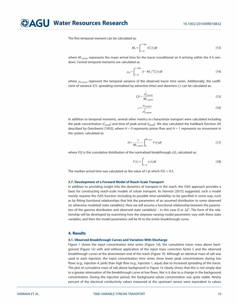
The shape of the seven breakthrough curves varied considerably over the course of the experiment (Figure1f). Breakthrough curves during lower discharge conditions were generally characterized by lower peakconcentrations, later mean arrival times, later time to peak concentration, decreased coefficient of variation(spreading relative to travel time), decreased skewness, and decreased holdback (Figure 2). Note that thesebreakthrough curve metrics are affected by the finite duration of the breakthrough curve observation (4 h)and the overprinting of the tail of each breakthrough curve by the breakthrough of the subsequent injec-tions (i.e., the stream did not return to the background level).

4.2. Structure of the Fitted rSAS FunctionsThe stepwise-varying rSAS function is able to produce predictions almost identical to the observations (Fig-ure 3). Table 1 gives the four parameter values fit to each slug, along with the calculated values of Sr and b,and the root-mean-square error (RMSE) and Nash-Sutcliffe model efficiency (NSE) for each of the seveninjection periods. The best fit RMSE was between 0.13 and 0.37 mg/L and the NSE is more than 0.995 for allseven periods (a NSE of 1 represents a perfect fit). The shape of the stepwise-varying rSAS function is illus-trated in Figure 3.

The uncertainty in the shape parameter a and scale parameter b are both considerably greater than theuncertainty in the mean and standard deviation Sl and Sr, which are tightly constrained by the break-through curve data. The mean of the fitted rSAS function begins at Sl 5 3.0 m3 during the first period, risesto a maximum of 5.0 m3 in the fourth period, and then declines. The standard deviation Sr rises quicklyover the first few periods, peaks in event three, and then slowly declines. These variations produce a distinctelongation and shift in the mode of the rSAS function toward larger ST, implying that the outflow contains alarger fraction of older water during periods 4, 5, and 6, when flow is lowest. Variations in Smin values from

Figure 2. Comparison of breakthrough curve summary metrics for the observed breakthrough, and for the four modeled cases.



slug to slug were smaller, and the uncertainties were larger, so it is not immediately clear whether thisparameter shifts significantly in time.

4.3. Internal and External Transit Time Variability, and Effects on Breakthrough CurvesThe importance of internal and external variability is illustrated in Figure 4. The results are shown for modelswhere both types of variability are accounted for, and with external variability only, internal variability only,and with neither type of variability. Note that when internal variability is removed (Figure 4, second andfourth rows), the rSAS function is invariant in time, by definition. The presence of external variability (Figure

Figure 3. Parameter estimation for the gamma distribution rSAS function fit to reproduce the breakthrough curve of each breakthrough curve. Dotty plots on the left show the Nash Sut-cliffe Efficiency (NSE) of the Monte-Carlo parameter estimates. The rSAS functions given by the best fit parameters are shown on the right. The distribution can be specified by the offsetSmin (given by the triangle), the mean (square), and the standard deviation (indicated by left-pointing and right-pointing triangles).

Table 1. Value of the rSAS Distribution Parameters for the Best Fit Stepwise rSAS Model, Where the Parameters are Allowed to Vary in aStepwise Way at the Moment Each of the Seven Tracer Injections Occurred, Along With the Root-Mean-Square Error (RMSE) and Nash-Sutcliffe Efficiency (NSE) Calculated for Each Perioda

a b (L) Smin (L) Sl (L) Sr (L) f (%)RMSE

(mg/L) NSE

Slug 1 1.44 (210/43%) 1465 (234/21%) 849 (222/7%) 2953 (211/7%) 1756 (221/14%) 19 0.35 0.9971Slug 2 1.34 (210/20%) 2036 (220/15%) 908 (213/10%) 3641 (26/5%) 2359 (212/9%) 36 0.36 0.9959Slug 3 1.42 (26/8%) 2609 (29/10%) 957 (212/4%) 4669 (23/3%) 3112 (27/7%) 53 0.30 0.9963Slug 4 2.00 (214/24%) 2137 (220/21%) 754 (235/21%) 5019 (27/7%) 3019 (212/12%) 91 0.14 0.9985Slug 5 1.95 (215/28%) 2123 (221/17%) 806 (243/23%) 4945 (26/5%) 2964 (211/10%) 68 0.13 0.9990Slug 6 1.97 (218/38%) 1840 (228/28%) 845 (248/25%) 4473 (29/9%) 2584 (217/17%) 40 0.23 0.9977Slug 7 1.21 (212/17%) 2421 (216/27%) 931 (212/9%) 3862 (27/11%) 2664 (211/19%) 27 0.31 0.9973Fixed 1.51 2296 870 4333 2820 1.69 0.9179

aParameters with units are given in liters. The overall RMSE was 0.29 mg/L and NSE was 0.9976. Uncertainty in each parameter is giv-en by the range of values for which the NSE> 0.99, expressed as percentage change (6%) from the best fit value.



4, second row) means that more discharge is removed from some age-ranks in storage at high flows thanlow flows, but the proportion of discharge from those parts of the storage is invariant. When external vari-ability is absent (Figure 4, third and fourth rows), the rSAS and complementary rSAS functions are identicalup to a scalar multiple (discharge) and constant offset (relative storage).

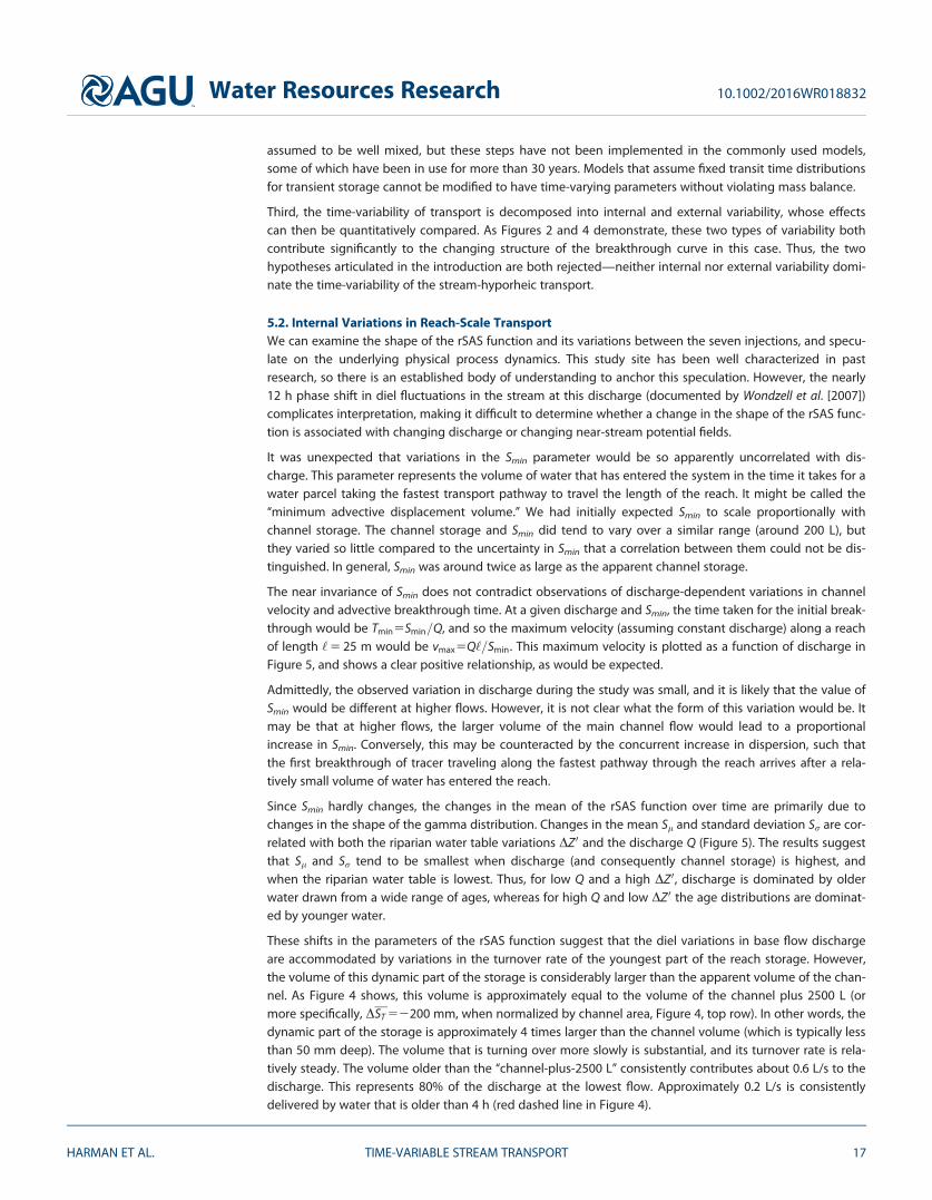
The plots of the complementary rSAS function for best fit case (Figure 4, top row, center plot) show an inter-esting behavior. Below about 2200 mm of age-ranked storage (equal to about 22500 L of storage in thereach), the rate of discharge is more or less constant at around 0.6 L s21. This suggests that during thehigher flow periods (at the start and end of the observed period), the variations in discharge are primarilyaccommodated by more rapidly turning over the younger storage. The slower flow pathways are relativelyunperturbed by an increase in streamflow. In fact, the results suggest that the rate of discharge from theolder storages declines when overall flow rate increases.

NSE > 0.99

NSE = 0.92

NSE = 0.90

NSE = 0.71

Q Q

2010-08-16 2010-08-17 2010-08-16 2010-08-17

Figure 4. Plots showing (left, center) the structure of the rSAS function and (right) the predicted (colored) and observed (gray) breakthrough curves, along with their residual error. Theresults are given for the best fit piecewise-varying rSAS function (top) for the case with only external and only internal variability and (bottom) for the case with no transport variability.Discharge is shown at the top of each column for reference. The left and center plots illustrate the structure of the storage selection in two different ways. Plots on the left show therSAS function as a density xðST ; tÞ (in the blue shaded contours) and as a cumulative distribution XðST ; tÞ (in the grey contours). Each of the rSAS functions in Figure 3 is equivalent to avertical slice through the top-left subplot in this figure. The center plots show the unnormalized complementary rSAS function in cumulative (QT ) and density (@QT =@DST ) forms (equa-tions (8) and (9), respectively). The area above the green line is the portion of storage younger than the first tracer injection, and the area above the red dashed line is younger than 4 h.Storage values in these plots have been normalized by the channel surface area (nominally 25 m 3 0.5 m) and converted to millimeters.



The observed breakthrough curves are best reproduced when both internal and external variability areaccounted for. When internal variability is removed (the fixed rSAS case) RMSE increases to 1.69 mg/L andNSE declines to 0.9. When external variability is removed (variable rSAS but constant flux Q0)RMSE 5 1.64 mg/L and NSE 5 0.91. When both are removed (fixed rSAS and constant flux Q0)RMSE 5 2.9 mg/L and NSE 5 0.71.

The effects are further illustrated by the metrics of breakthrough curve shape (Figure 2). The model runswith both internal and external variability generally match the observed metrics very well. These both tendto show a large U-shaped variation in breakthrough curve properties over the course of the seveninjections.

Removal of internal and/or external variability tends to flatten, if not completely reversed, this pattern ofvariation. For example, the observed time to peak concentration varies from 0.4 to 1.1 h, but when internalor external variability is removed the arrival times become less varied. When both are removed, the mod-eled time to peak becomes almost invariant. Similar patterns can be seen for the median arrival time, coeffi-cient of variation, skewness and holdback. The peak concentration goes further: when the variability isremoved the peak concentration is highest, rather than lowest, for the middle set of events.

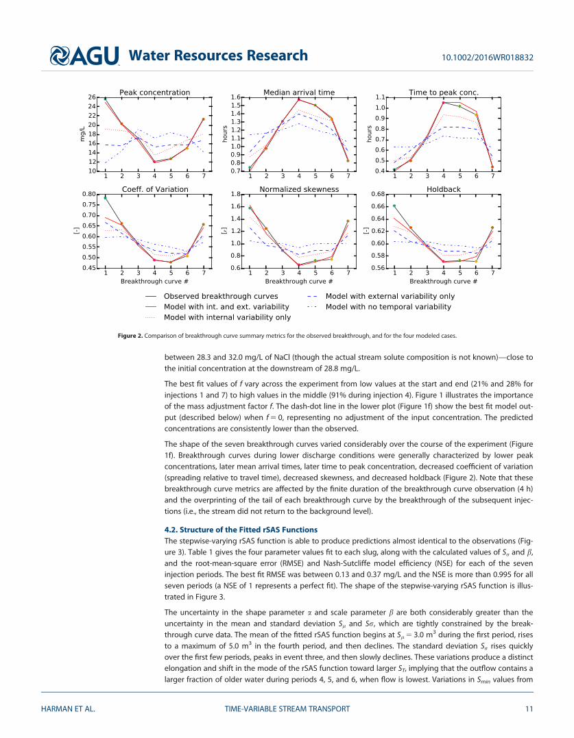
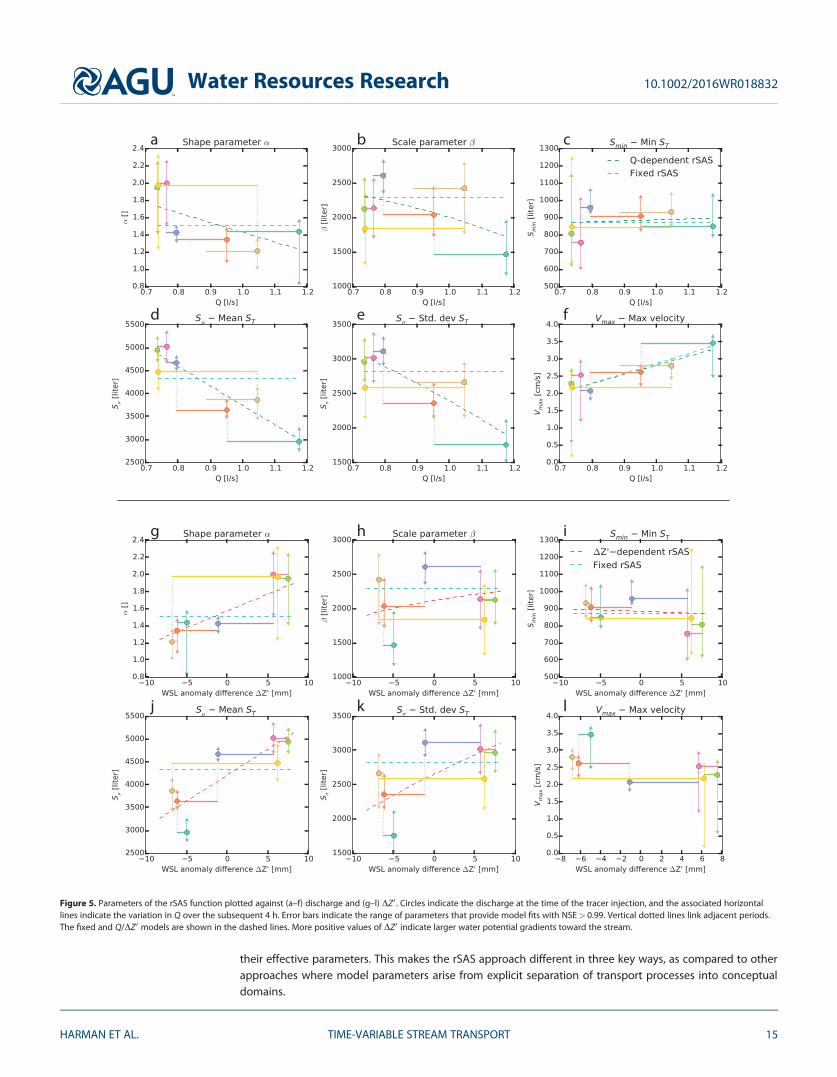
4.4. Correlation of rSAS Internal Variability With Discharge and Riparian Potential GradientsRelationships with Q and DZ0 are strongest for the central moments of the rSAS distribution, and weaker forthe parameters (Figure 5). The mean Sl increases systematically with DZ0, and decreases with Q. The stan-dard deviation Sr decreases with Q and shows some tendency to increase with DZ0, but the relationship isnot as strong. In contrast, the scale parameter b does not appear to vary systematically with either Q or DZ0.The high values of the shape parameter a in periods 4, 5, and 6 are associated with low (or increasing) Qand high (or decreasing) DZ0. The low values in the other events are associated with a range of Q, but seemto be clustered around low (or increasing) values of DZ0. Variations in Smin parameter are weak and generallysmaller than the range of values in the NSE> 0.99 bounds. The f parameter (Table 1) shows clearer relation-ships, decreasing with Q and increasing with DZ0.

The relationships shown in Figure 5 suggest that both state variables are typically better correlated with themoments of the distribution than with the parameters per se, and the correlations appear to be linear. Thus,to construct a forward model, we might assume functional relationships of the form:

Sl5alX1bl (19)

Sr5arX1br (20)

Smin5aminX1bmin (21)

where X is either DQ (the variation in discharge around the mean, Q2�Q) or DZ0. Values of the a and bparameters were calibrated by minimizing the RMSE error with the observed breakthrough curve concen-trations. The resulting models relating rSAS parameters to Q or DZ0 are also plotted in Figure 5, along withthe fixed rSAS parameters for comparison, and the best fit model parameters are given in Table 2.

Results demonstrate that models based on Q and DZ0 perform similarly (which is unsurprising given theircovariation) at a level somewhat below that of the piecewise-varying rSAS (Nash-Sutcliffe efficiency of 0.97–0.98 rather than >0.99) but considerably better than the fixed rSAS (0.92). The effects on the predicted rSASfunction and breakthrough curve predictions are given in Figure 6. Both models are able to reproduce themajor features of the rSAS function and match the breakthrough curves well. Much of the error seems to beassociated with the timing of the initial breakthrough. This was expected, since the timing is controlled bySmin, and this parameter had relatively little relationship to the observed state variables.

5. Discussion

5.1. rSAS as a Process-Agnostic Interpretation FrameworkAs demonstrated above, reach-scale transport dynamics can be reproduced by the rSAS model. This sup-ports the use of rSAS as a method for analyzing and interpreting stream solute tracer studies in a ‘‘process-agnostic’’ way. We describe the rSAS framework as process-agnostic in the sense that the key outcome isthe rank Storage Selection function, which is not based on a suite of conceptual storages and fluxes and



their effective parameters. This makes the rSAS approach different in three key ways, as compared to otherapproaches where model parameters arise from explicit separation of transport processes into conceptualdomains.

a b c

d e f

g h i

j k l

Figure 5. Parameters of the rSAS function plotted against (a–f) discharge and (g–l) DZ0 . Circles indicate the discharge at the time of the tracer injection, and the associated horizontallines indicate the variation in Q over the subsequent 4 h. Error bars indicate the range of parameters that provide model fits with NSE> 0.99. Vertical dotted lines link adjacent periods.The fixed and Q/DZ0 models are shown in the dashed lines. More positive values of DZ0 indicate larger water potential gradients toward the stream.



First, the rSAS approach treats thestream-hyporheic system as a con-tinuum rather than as distinctdomains with different process rep-resentations. In contrast, commonframeworks such as the transientstorage model [Bencala and Walters,1983], Advection Storage-Path mod-el [Worman et al., 2002], andSTAMMT-L [Haggerty et al., 2000]assign specific advective, dispersive,

and storage processes to distinct domains. In these models, streams are represented as a one-dimensionaldomain with advection and longitudinal dispersion. Transient storage may be represented as an additionalsingle domain or multiple domains [Kerr et al., 2013; Briggs et al., 2009; Choi et al., 2000], each of which ischaracterized by some specified transit time distribution. There is considerable overlap in the time scales ofretention in in-stream transient storage and in rapid hyporheic exchange. Thus, (1) both can simultaneouslyact on breakthrough curves, (2) their effects cannot be distinguished based on in-stream observations alone[Kelleher et al., 2013], and (3) model storage domains cannot be explicitly said to be surface or subsurfacestorage domains. The rSAS approach represents the system as a continuum of age-ranked storage, varyingfrom the advection-dominated stream (the most mobile water, and most preferentially sampled in ourresults; the top of Figure 4) to the water that is functionally immobile during the experiment (the leastmobile water, minimally sampled in our study; the bottom of Figure 4).

Second, the rSAS framework accounts for the effect of internal variability on transit time distributionsthroughout the system. Transport processes such as dispersion and groundwater discharge into streamsare expected to vary with discharge. The existing models outlined above have primarily been applied dur-ing steady flow conditions where the parameters describing processes are fixed in time. One notable excep-tion is the unsteady state flow routing coupled to the transient storage model implemented by Runkel et al.[1998], where stream area and discharge were allowed to vary in time, but all other transport parameters(representing dispersion and transient storage) were fixed. The ability to continuously vary all parameterswith discharge could be implemented in those existing models where conceptual compartments are

Table 2. Alternative Models of the rSAS Model Parameters and Their AssociatedPerformancesa

Model Parameter Submodels RMSE (mg/L) NSE

Discharge Sl ðLÞ524084:62 ðQ2�QÞ14279:39 0.75 0.9739SrðLÞ522431:81 ðQ2�QÞ12698:59SminðLÞ559:51 ðQ2�QÞ1873:64

Riparian SlðLÞ5112:54 DZ014197:71 0.66 0.9771SrðLÞ558:37 DZ012628:58SminðLÞ521:78 DZ01876:47

aQ in liter per second, DZ0 in millimeter, f in percentage, and Smin and Sl in liter.Mean discharge is �Q50:870 L/s.

Q Q

NSE = 0.97

NSE = 0.98

2010-08-16 2010-08-17 2010-08-16 2010-08-17 2010-08-16 2010-08-17

Figure 6. Similar plots to Figure 4 but with rSAS functions predicted from (top) the discharge and (bottom) the riparian water table elevation. Discharge is shown at the top of each col-umn for reference.



assumed to be well mixed, but these steps have not been implemented in the commonly used models,some of which have been in use for more than 30 years. Models that assume fixed transit time distributionsfor transient storage cannot be modified to have time-varying parameters without violating mass balance.

Third, the time-variability of transport is decomposed into internal and external variability, whose effectscan then be quantitatively compared. As Figures 2 and 4 demonstrate, these two types of variability bothcontribute significantly to the changing structure of the breakthrough curve in this case. Thus, the twohypotheses articulated in the introduction are both rejected—neither internal nor external variability domi-nate the time-variability of the stream-hyporheic transport.

5.2. Internal Variations in Reach-Scale TransportWe can examine the shape of the rSAS function and its variations between the seven injections, and specu-late on the underlying physical process dynamics. This study site has been well characterized in pastresearch, so there is an established body of understanding to anchor this speculation. However, the nearly12 h phase shift in diel fluctuations in the stream at this discharge (documented by Wondzell et al. [2007])complicates interpretation, making it difficult to determine whether a change in the shape of the rSAS func-tion is associated with changing discharge or changing near-stream potential fields.

It was unexpected that variations in the Smin parameter would be so apparently uncorrelated with dis-charge. This parameter represents the volume of water that has entered the system in the time it takes for awater parcel taking the fastest transport pathway to travel the length of the reach. It might be called the‘‘minimum advective displacement volume.’’ We had initially expected Smin to scale proportionally withchannel storage. The channel storage and Smin did tend to vary over a similar range (around 200 L), butthey varied so little compared to the uncertainty in Smin that a correlation between them could not be dis-tinguished. In general, Smin was around twice as large as the apparent channel storage.

The near invariance of Smin does not contradict observations of discharge-dependent variations in channelvelocity and advective breakthrough time. At a given discharge and Smin, the time taken for the initial break-through would be Tmin5Smin=Q, and so the maximum velocity (assuming constant discharge) along a reachof length ‘5 25 m would be vmax5Q‘=Smin. This maximum velocity is plotted as a function of discharge inFigure 5, and shows a clear positive relationship, as would be expected.

Admittedly, the observed variation in discharge during the study was small, and it is likely that the value ofSmin would be different at higher flows. However, it is not clear what the form of this variation would be. Itmay be that at higher flows, the larger volume of the main channel flow would lead to a proportionalincrease in Smin. Conversely, this may be counteracted by the concurrent increase in dispersion, such thatthe first breakthrough of tracer traveling along the fastest pathway through the reach arrives after a rela-tively small volume of water has entered the reach.

Since Smin hardly changes, the changes in the mean of the rSAS function over time are primarily due tochanges in the shape of the gamma distribution. Changes in the mean Sl and standard deviation Sr are cor-related with both the riparian water table variations DZ0 and the discharge Q (Figure 5). The results suggestthat Sl and Sr tend to be smallest when discharge (and consequently channel storage) is highest, andwhen the riparian water table is lowest. Thus, for low Q and a high DZ0, discharge is dominated by olderwater drawn from a wide range of ages, whereas for high Q and low DZ0 the age distributions are dominat-ed by younger water.

These shifts in the parameters of the rSAS function suggest that the diel variations in base flow dischargeare accommodated by variations in the turnover rate of the youngest part of the reach storage. However,the volume of this dynamic part of the storage is considerably larger than the apparent volume of the chan-nel. As Figure 4 shows, this volume is approximately equal to the volume of the channel plus 2500 L (ormore specifically, DST 52200 mm, when normalized by channel area, Figure 4, top row). In other words, thedynamic part of the storage is approximately 4 times larger than the channel volume (which is typically lessthan 50 mm deep). The volume that is turning over more slowly is substantial, and its turnover rate is rela-tively steady. The volume older than the ‘‘channel-plus-2500 L’’ consistently contributes about 0.6 L/s to thedischarge. This represents 80% of the discharge at the lowest flow. Approximately 0.2 L/s is consistentlydelivered by water that is older than 4 h (red dashed line in Figure 4).



The extent to which the variations in the riparian water table contribute to this pattern is not clear. Previousstudies have suggested that high riparian water tables could be associated with a contraction of the hypo-rheic zone [Cardenas and Wilson, 2007; Cardenas, 2009; Storey et al., 2003]. Here in contrast, the apparent vol-ume turning over most quickly is largest in the middle of the experiment, when the riparian water tables arehighest. Furthermore, as Figure 4 shows, the apparent turnover rate in the older part of the storage may behigher during the high-water table period (indicated by the downward deflection of the 0.2 L/s contour in thetop center figure). This is inconsistent with an immobilization of older water when the riparian water table ishigh. This observation is close to the edge of the window of detection of the experiment (i.e., the 4 h agedwater indicated by the red dashed line in Figure 4), and so this result cannot be considered conclusive. It mayin fact be an artifact of the gamma-distribution functional form—the increased relative discharge above DST

52200 mm requires the function to ‘‘pivot,’’ reducing the amount of discharge below DST 52200 mm. Moresophisticated functional forms for the rSAS function must be explored to examine this possibility.

5.3. Toward a Time-Variable rSAS Parameterization at the Reach ScaleThe results also indicated the feasibility of using rSAS as a basis for forward modeling of reach-scale trans-port. As an illustration of how this type of model can be used, the discharge-dependent model was appliedto the 4 days up to and including the study period. Discharge over that period varies over a consistentrange, so the results do not require extrapolation of the model relationships. The results are shown in Figure7. The top and bottom contour plots correspond to the left and right plots in Figures 4 and 6. The plots onthe right summarize how discharge is extracted from storage over the modeled periods. These distributions

2010-08-14 2010-08-15 2010-08-16 2010-08-17

Figure 7. Structure of the rSAS function predicted from observed discharge over a 4 day period up to and including the study period.Study period is highlighted in grey in the top figure. Contour plots show (top) the rSAS function XðST ; tÞ and (bottom) the QT ðDST ; tÞ func-tion. Plots on the right show the mean and standard deviation of the density forms of the functions at each value of ST and DST .



show that the pattern identified for the experimental period is repeated in time. Most of the time-variabledischarge is drawn from the youngest DST > 2200 part of the storage, and discharge from DST < 2200 isrelatively steady, apart from a reduction during the high flows (which may be artifactual).

To extend this kind of modeling approach to other hydraulic conditions and other reaches where tracerdata are not available, we must understand the relationship between the rSAS function and the physicalstructure of stream reaches. There is good reason to hope that such a mapping from landscape to model ispossible, since the rSAS function is a distribution over the real storage volume of water within the reach.Thus investigation of the rSAS function can proceed by identifying how age-ranked storage is distributed inspace, and how the transport processes operating within the reach determine the shape of the rSAS func-tion. For example, a more accurate survey of in-channel volume would help determine the extent to whichin-channel transient storage (for instance, in pools and eddies unrepresented by the crude channel volumeestimate used here) is sufficient to fully account for the 200 mm of dynamic turnover storage. Subsurfaceobservations of storage and/or transport could also be used to determine the volume in the bed that isturning over on those time scales, and thus map the age-rank storage back into the landscape.

6. Conclusions and Future Research

This application of the rank Storage Selection (rSAS) theory to a sequence of tracer breakthrough curves ina small stream has demonstrated the ability of this approach to reproduce the observed transport dynam-ics, to provide insight into the time-varying turnover of storage volumes within the reach, and to examinethe covariation of that internal variability with the controlling state variables.

Rather than support one of the ‘‘contradictory’’ hypotheses established in the introduction to this paper, theresults suggest that both internal and external variability control the temporal variability of transit timesthrough the reach. The diel increases in discharge are accommodated in the reach by an increase in theturnover rate of a volume of water approximately 4 times larger than the channel. In addition, a large por-tion of the discharge is supplied by turnover of older water, and the rate of that turnover is relatively unper-turbed by the variations in discharge. This likely represents Darcian flow through the hyporheic zone drivenby the (relatively unchanging) topographic gradient of the valley bottom. Variations in the turnover of theseslower flow paths are unlikely to be driven by variations in riparian water tables, and may be artifacts.

We have also shown that this approach can be used to construct a model of the time-varying rSAS functionin terms of the observed state variables of discharge and riparian water table elevations. These modelswere able to similarly reproduce the transport dynamics. As such, we believe this approach holds promiseas a basis for constructing reach-scale transport models that can act as elements of a time-variable solutetransport models at the network scale.

ReferencesAbramowitz, M., and I. A. Stegun (1964), Handbook of Mathematical Functions: With Formulas, Graphs, and Mathematical Tables, vol. 55,

Dover Publications Inc., N. Y.Bencala, K. E., and R. A. Walters (1983), Simulation of solute transport in a mountain pool-and-riffle stream: A transient storage model,

Water Resour. Res., 19(3), 718–724, doi:10.1029/WR019i003p00718.Bencala, K. E., M. N. Gooseff, and B. A. Kimball (2011), Rethinking hyporheic flow and transient storage to advance understanding of

stream-catchment connections, Water Resour. Res., 47, W00H03, doi:10.1029/2010WR010066.Botter, G., E. Bertuzzo, and A. Rinaldo (2010), Transport in the hydrologic response: Travel time distributions, soil moisture dynamics, and

the old water paradox, Water Resour. Res., 46, W03514, doi:10.1029/2009WR008371.Briggs, M. A., M. N. Gooseff, C. D. Arp, and M. A. Baker (2009), A method for estimating surface transient storage parameters for streams

with concurrent hyporheic storage, Water Resour. Res., 45, W00D27, doi:10.1029/2008WR006959.Cardenas, M. B. (2009), Stream-aquifer interactions and hyporheic exchange in gaining and losing sinuous streams, Water Resour. Res., 45,

W06429, doi:10.1029/2008WR007651.Cardenas, M. B., and J. L. Wilson (2007), Exchange across a sediment-water interface with ambient groundwater discharge, J. Hydrol., 346(3-

4), 69–80, doi:10.1016/j.jhydrol.2007.08.019.Choi, J., J. W. Harvey, and M. H. Conklin (2000), Characterizing multiple timescales of stream and storage zone interaction that affect solute

fate and transport in streams, Water Resour. Res., 36(6), 1511–1518.Danckwerts, P. V. (1953), Continuous flow systems: Distribution of residence times, Chem. Eng. Sci., 2(1), 1–13.Day, T. J. (1977), Field procedures and evaluation of a slug dilution gauging method in mountain streams, J. Hydrol. N. Z., 16(2), 113–133.Dudley-Southern, M., and A. Binley (2015), Temporal responses of groundwater-surface water exchange to successive storm events, Water

Resour. Res., 51, 1112–1126, doi:10.1002/2014WR016623.Dymess, C. T. (1969), Hydrologic properties of soils on three small watersheds in the western Cascades of Oregon, USDA For. Ser. Res. Note

PNW-111, 17 pp., Pacific Northwest Forest and Range Experiment Station, Portland, Oreg.

AcknowledgmentsThanks to Celine Cua for contributionsto data analysis. C. J. Harmanacknowledges the support of NSFgrants NSF EAR-1344664 and CBET-1360415. Ward was supported by theNSF grant EAR-0911435. Tools forsolute tracer time series analyses weredeveloped by Ward and others withsupport provided in part by the NSFgrant EAR 1331906 for the CriticalZone Observatory for IntensivelyManaged Landscapes (IML-CZO), amulti-institutional collaborative effort.Ward was also supported by theIndiana University Office of the ViceProvost for Research. Data andfacilities were provided by the H.J.Andrews Experimental Forest researchprogram, funded by the NSFs Long-Term Ecological Research Program(DEB-1440409), US Forest ServicePacific Northwest Research Station,and Oregon State University. Anyopinions, findings, and conclusions orrecommendations expressed in thismaterial are those of the authors anddo not necessarily reflect the views ofthe National Science Foundation, U.S.Forest Service, H.J. AndrewsExperimental Forest, Oregon StateUniversity, or Indiana University.Discharge data are available from theH.J. Andrews Experimental Forest DataCatalog (http://andrewsforest.oregonstate.edu/). In-stream specificconductance time series are availableupon request to Ward ([email protected]). The authors declare noconflicts of interest.



http://dx.doi.org/10.1029/WR019i003p00718

http://dx.doi.org/10.1029/2010WR010066

http://dx.doi.org/10.1029/2009WR008371

http://dx.doi.org/10.1029/2008WR006959

http://dx.doi.org/10.1029/2008WR007651

http://dx.doi.org/10.1016/j.jhydrol.2007.08.019

http://dx.doi.org/10.1002/2014WR016623

http://andrewsforest.oregonstate.edu

http://andrewsforest.oregonstate.edu

Fischer, H. B., J. E. List, C. R. Koh, J. Imberger, and N. H. Brooks (1979), Mixing in Inland and Coastal Waters, Academic, San Diego, Calif.Gooseff, M. N., K. E. Bencala, and S. M. Wondzell (2008), Solute transport along stream and river networks, in River Confluences, Tributaries,

and the Fluvial Network, edited by S. P. Rice, A. G. Roy, and B. L. Rhoads, pp. 395–418, John Wiley, Hoboken, N. J.Haggerty, R., S. A. McKenna, and L. C. Meigs (2000), On the late-time behavior of tracer test breakthrough curves, Water Resour. Res., 36(12),

3467–3479, doi:10.1029/2000WR900214.Harman, C. J. (2015), Time-variable transit time distributions and transport: Theory and application to storage-dependent transport of chlo-

ride in a watershed, Water Resour. Res., 51, 1–30, doi:10.1002/2014WR015707.Harvey, J. W., and K. E. Bencala (1993), The Effect of streambed topography on surface-subsurface water exchange in mountain catch-

ments, Water Resour. Res., 29(1), 89–98.Harvey, J. W., B. J. Wagner, and K. E. Bencala (1996), Evaluating the reliability of the stream tracer approach to characterize stream-

subsurface water exchange, Water Resour. Res., 32(8), 2441–2451, doi:10.1029/96WR01268.Jones, E., T. Oliphant, and P. Peterson (2001), SciPy: Open source scientific tools for Python. [Available at http://www.scipy.org/.]Kelleher, C., T. Wagener, B. McGlynn, A. S. Ward, M. N. Gooseff, and R. A. Payn (2013), Identifiability of transient storage model parameters

along a mountain stream, Water Resour. Res., 49, 5290–5306, doi:10.1002/wrcr.20413.Kerr, P. C., M. N. Gooseff, and D. Bolster (2013), The significance of model structure in one-dimensional stream solute transport models with mul-

tiple transient storage zones—Competing vs. nested arrangements, Remote Sens. Environ., 497, 133–144, doi:10.1016/j.jhydrol. 2013.05.013.Kim, M., L. Pangle, C. Cardoso, M. Lora, T. Volkmann, Y. Wang, C. Harman, and P. Troch (2016), Transit time distributions and StorAge Selec-

tion functions in a variably-saturated sloping soil lysimeter: Direct observation of internal and external transport variability, WaterResour. Res., doi:10.1002/2016WR018620, in press.

Kirchner, J. W., X. Feng, and C. Neal (2000), Fractal stream chemistry and its implications for contaminant transport in catchments, Nature,403(6769), 524–527, doi:10.1038/35000537.

Leopold, L. B., and T. Maddock (1953), The hydraulic geometry of stream channels and some physiographic implications, technical report,U.S. Dep. of the Inter., U.S. Geol. Surv. Geological Survey Professional Paper 252, United States Government Printing Office, Washington, D. C.

Loheide, S. P., and J. D. Lundquist (2009), Snowmelt-induced diel fluxes through the hyporheic zone, Water Resour. Res., 45, W07404, doi:10.1029/2008WR007329.

Malzone, J. M., and C. S. Lowry (2014), Focused groundwater controlled feedbacks into the hyporheic zone during baseflow recession,Ground Water, 53(2), 217–226, doi:10.1111/gwat.12186.

Payn, R. A., M. N. Gooseff, B. L. McGlynn, K. E. Bencala, and S. M. Wondzell (2009), Channel water balance and exchange with subsurfaceflow along a mountain headwater stream in Montana, United States, Water Resour. Res., 45, W11427, doi:10.1029/2008WR007644.

Rinaldo, A., K. J. Beven, E. Bertuzzo, L. Nicotina, J. Davies, A. Fiori, D. Russo, and G. Botter (2011), Catchment travel time distributions andwater flow in soils, Water Resour. Res., 47, W07537, doi:10.1029/2011WR010478.

Rinaldo, A., P. Benettin, C. J. Harman, M. Hrachowitz, K. J. McGuire, Y. van der Velde, E. Bertuzzo, and G. Botter (2015), Storage selectionfunctions: A coherent framework for quantifying how catchments store and release water and solutes, Water Resour. Res., 51, 4840–4847, doi:10.1002/2015WR017273.

Rodhe, A., L. Nyberg, and K. Bishop (1996), Transit times for water in a small till catchment from a step shift in the oxygen 18 content ofthe water input, Water Resour. Res., 32(12), 3497–3511, doi:10.1029/95WR01806.

Runkel, R. L., D. M. McKnight, and E. D. Andrews (1998), Analysis of transient storage subject to unsteady flow: Diel flow variation in an Ant-arctic stream, J. North Am. Benthol. Soc., 17(2), 143–154.

Sawyer, A. H., and M. B. Cardenas (2009), Impact of dam operations on hyporheic exchange in the riparian zone of a regulated river, Hydrol.Processes, 23, 2129–2137, doi:10.1002/hyp.7324.

Sawyer, A. H., F. Shi, J. T. Kirby, and H. A. Michael (2013), Dynamic response of surface water-groundwater exchange to currents, tides, andwaves in a shallow estuary, J. Geophys. Res. Oceans, 118, 1749–1758, doi:10.1002/jgrc.20154.

Schmadel, N. M., et al. (2016), Stream solute tracer timescales changing with discharge and reach length confound process interpretation,Water Resour. Res., 52, 3227–3245, doi:10.1002/2015WR018062.

Stanford, J. A., and J. V. Ward (1993), An ecosystem perspective of alluvial rivers: Connectivity and the hyporheic corridor, J. North Am. Ben-thol. Soc., 12(1), 48–60.

Storey, R. G., K. W. F. Howard, and D. D. Williams (2003), Factors controlling riffle-scale hyporheic exchange flows and their seasonalchanges in a gaining stream: A three-dimensional groundwater flow model, Water Resour. Res., 39(2), 1034, doi:10.1029/2002WR001367.

Swanson, F. J., and M. E. James (1975), Geology and geomorphology of the H.J. Andrews Experimental Forest, western Cascades, Oregon,technical report USDA For. Ser. PNW-188, 14 pp., Pacific Northwest Forest and Range Experiment Station, Portland, Oreg.

Swanson, F. J., and J. A. Jones (2002), Geomorphology and hydrology of the HJ Andrews experimental forest, Blue River, Oregon, in FieldGuide to Geologic Processes in Cascadia: Field Trips to Accompany the 98th Annual Meeting of the Cordilleran Section of the Geological Soci-ety of America, vol. 36, edited by G. W. Moore, pp. 289–314, Oregon Department of Geology and Mineral Industries, Portland, Oreg.

van der Velde, Y., P. J. J. F. Torfs, S. E. A. T. M. van der Zee, and R. Uijlenhoet (2012), Quantifying catchment-scale mixing and its effect ontime-varying travel time distributions, Water Resour. Res., 48, W06536, doi:10.1029/2011WR011310.

Vannote, R. L., G. W. Minshall, K. W. Cummins, J. R. Sedell, and C. E. Cushing (1980), The river continuum concept, Can. J. Fish. Aquat. Sci., 37,130–137.

Voltz, T., M. N. Gooseff, A. S. Ward, K. Singha, M. Fitzgerald, and T. Wagener (2013), Riparian hydraulic gradient and stream-groundwaterexchange dynamics in steep headwater valleys, J. Geophys. Res. Earth Surf., 118, 953–969, doi:10.1002/jgrf.20074.

Wagner, B. J., and J. W. Harvey (1997), Experimental design for estimating parameters of rate-limited mass transfer: Analysis of stream trac-er studies, Water Resour. Res., 33(7), 1731–1741, doi:10.1029/97WR01067.

Ward, A. S., M. Fitzgerald, M. N. Gooseff, T. J. Voltz, A. M. Binley, and K. Singha (2012), Hydrologic and geomorphic controls on hyporheicexchange during base flow recession in a headwater mountain stream, Water Resour. Res., 48, W04513, doi:10.1029/2011WR011461.

Ward, A. S., M. N. Gooseff, T. J. Voltz, M. Fitzgerald, K. Singha, and J. P. Zarnetske (2013a), How does rapidly changing discharge duringstorm events affect transient storage and channel water balance in a headwater mountain stream?, Water Resour. Res., 49, 5473–5486,doi:10.1002/wrcr.20434.

Ward, A. S., R. A. Payn, M. N. Gooseff, B. L. McGlynn, K. E. Bencala, C. A. Kelleher, S. M. Wondzell, and T. Wagener (2013b), Variations in sur-face water-ground water interactions along a headwater mountain stream: Comparisons between transient storage and water balanceanalyses, Water Resour. Res., 49, 3359–3374, doi:10.1002/wrcr.20148.

Ward, A. S., N. M. Schmadel, S. M. Wondzell, C. J. Harman, M. N. Gooseff, and K. Singha (2016), Hydrogeomorphic controls on hyporheicand riparian transport in two headwater mountain streams during base flow recession, Water Resour. Res., 52, 1479–1497, doi:10.1002/2015WR018225.



http://dx.doi.org/10.1029/2000WR900214

http://dx.doi.org/10.1002/2014WR015707

http://dx.doi.org/10.1029/96WR01268

http://onlinelibrary.wiley.com/doi/http://www.scipy.org/

http://dx.doi.org/10.1002/wrcr.20413

http://dx.doi.org/10.1016/j.jhydrol

http://dx.doi.org/10.1002/2016WR018620

http://dx.doi.org/10.1038/35000537

http://dx.doi.org/10.1029/2008WR007329

http://dx.doi.org/10.1111/gwat.12186

http://dx.doi.org/10.1029/2008WR007644

http://dx.doi.org/10.1029/2011WR010478

http://dx.doi.org/10.1002/2015WR017273


http://dx.doi.org/10.1002/hyp.7324

http://dx.doi.org/10.1002/jgrc.20154

http://dx.doi.org/10.1002/2015WR018062

http://dx.doi.org/10.1029/2002WR001367

http://dx.doi.org/10.1029/2011WR011310

http://dx.doi.org/10.1002/jgrf.20074


http://dx.doi.org/10.1029/2011WR011461



http://dx.doi.org/10.1002/2015WR018225

http://dx.doi.org/10.1002/2015WR018225

Wondzell, S. M. (2006), Effect of morphology and discharge on hyporheic exchange flows in two small streams in the Cascade Mountainsof Oregon, USA, Hydrol. Processes, 20(2), 267–287, doi:10.1002/hyp.5902.

Wondzell, S. M., M. N. Gooseff, and B. L. McGlynn (2007), Flow velocity and the hydrologic behavior of streams during baseflow, Geophys.Res. Lett., 34, L24404, doi:10.1029/2007GL031256.

Wondzell, S. M., M. N. Gooseff, and B. L. McGlynn (2009a), An analysis of alternative conceptual models relating hyporheic exchange flowto diel fluctuations in discharge during baseflow recession, Hydrol. Processes, 24(6), 686–694, doi:10.1002/hyp.7507.

Wondzell, S. M., J. LaNier, and R. Haggerty (2009b), Evaluation of alternative groundwater flow models for simulating hyporheic exchangein a small mountain stream, J. Hydrol., 364(1–2), 142–151, doi:10.1016/j.jhydrol.2008.10.011.

Worman, A., A. I. Packman, H. Johansson, and K. Jonsson (2002), Effect of flow-induced exchange in hyporheic zones on longitudinal trans-port of solutes in streams and rivers, Water Resour. Res., 38(1), doi:10.1029/2001WR000769.




http://dx.doi.org/10.1029/2007GL031256


http://dx.doi.org/10.1016/j.jhydrol.2008.10.011

http://dx.doi.org/10.1029/2001WR000769

how does reach‐scale stream‐hyporheic transport vary with...

Documents