How Firms Accumulate Inputs:

Evidence from Import Switching∗

Dan Lu1, Asier Mariscal2, and Luis-Fernando Mejıa3

1University of Rochester2University of Alicante

3National Planning Department, Colombia

May 11, 2016

Abstract

We uncover new dynamic patterns, related to importers’ age and the overall macroeconomic environment,

that static models cannot explain. Our findings are related to imported inputs switching, i.e., the simultaneous

adding and dropping of intermediates at the firm level. Three facts stand out. First, switching is pervasive

and a sizable fraction of firms’ import. Second, conditional on age, larger firms are more likely to switch.

Conditional on size, younger firms switch more. Third, when import prices are high, fewer firms switch and

share of switched inputs falls. We propose a dynamic model, where firms search for foreign suppliers and

face a choice over heterogeneously productive intermediate goods. Through this process, firms improve their

productivity and grow over time. Finally, we show that several key predictions of the model hold using

regressions that exploit informative within-firm variation. First, least productive intermediates are more likely

to be dropped. Second, over time firms increase the number of foreign intermediates used, and reduce their

switching. Third, switching leads to a quantitatively significant growth in future sales. We view our paper as

complementary to those that emphasize capital accumulation and worker reallocation as important drivers of

firm dynamics and aggregate productivity.

∗This paper is a substantial revision of our paper ”Import Switching and the Impact of a LargeDevaluation”. We would like to thank seminar and conference participants for comments on the earlyversion at Beijing University, Fedesarrollo, Hong Kong University, Penn State University, PhiladelphiaFED, Queen’s University, RMET, SED, University of Alicante and University of Rochester. We alsothank George Alessandria, Yan Bai, Mark Bils, Thomas Chaney, Harald Fadinger, Andreas Moxnesand Brent Neiman for very helpful comments and Alejo Forero for his excellent research assistance.Financial support from the Ministerio de Ciencia e Innovacion and FEDER funds is gratefully ac-knowledged.

1

1 Introduction

While sourcing inputs from abroad is important for firm productivity1, little work fo-

cuses on how firms’ accumulate them. This paper documents that a substantial number

of input varieties are simultaneously added and dropped at firm level, a phenomenon

called “switching,” using a sample of Colombian manufacturing firms. We show that

patterns in input switching depend on firms’ lifecycle and the macroeconomic environ-

ment. This evidence on switching sheds light on the ways in which firms accumulate

and upgrade their foreign inputs. Such findings cannot be explained by standard, static

models.

We start by describing three key facts which motivate this project. First, Colombian

manufacturing firms switch frequently their imported inputs. We find that, on average,

around 60% of firms switch inputs every year, while almost all firms in the 90th percentile

do. Conditional on switching, and by a conservative measure2, on average they add and

drop more than 30% of the value of their imported inputs. In the aggregate, each one

of these margins (adding and dropping) is also large, accounting for more than twice

the total changes in import value in the sample3. Second, in the data, conditional on

age, larger firms are more likely to switch. On the other hand, conditional on size,

younger firms switch more. Third, we find that switching is procyclical. Specifically,

there is more inaction during depreciation episodes: fewer firms switch, and firms that

do switch add and drop a lower share of inputs.

Switching involves adding and dropping imported input varieties, defined at a highly

disaggregated level. Accordingly, this can be seen as firms searching and substituting

some inputs or suppliers for others. Through this search process, firms’ use of imported

varieties will accumulate and change over time. From this perspective, the cross-section

and time-series patterns of firm-level switching suggest the existence of interesting dy-

namics on how firms accumulate foreign input varieties.

We propose a dynamic model of how firms accumulate foreign inputs, through the

search for more productive suppliers. The model extends the static model of endogenous

choice of imported inputs in Halpern et al. (2011) and Gopinath and Neiman (2011) by

1 See Amiti and Konings (2007), Goldberg et al. (2010), Halpern et al. (2011), Gopinath andNeiman (2011), etc.

2The measure is conservative in that it defines dropped imported inputs as those never boughtagain by the firm, whereas added products as those were never bought by the firm before.

3When including temporary additions and drops, each flow is about 8 times the change in importvalue.

2

introducing search and an adjustment of imported inputs over time. Firms’ production

function features love-of-variety in intermediates, while imports incur a convex cost.

Inputs are heterogeneous in their productivity and firms choose to import an endogenous

range of them. Searching for new inputs is costly, modeled as facing a fixed cost and

an adjustment cost: Together they allow for both an intensive and an extensive margin

of search. As a consequence, only the more productive firms search and when they find

new, more productive inputs, they substitute them for their old ones. In a nutshell, the

switching of inputs can be seen as firms searching for new suppliers and reorganizing

their production by changing imported inputs within narrowly defined categories.

The dynamic model can explain key empirical findings, in our Colombian sample and

the literature. First, in the data, most firms switch imported varieties and those that do

experience sales growth. In the model, firms pay a search cost to be connected with new

suppliers of foreign inputs, and shift their use of inputs towards the more productive

ones. Second, in the model, because the benefit from searching for new suppliers is larger

for more productive firms, bigger firms search and switch. Over time, firms use more

varieties and, since finding better suppliers gets harder and harder, older firms switch

less. Third, in the model, there is indeed more inaction when the import price is high,

because the gains from searching are diminished. This mechanism also suggests that

reducing import tariffs could lead to larger productivity gains and that devaluations

lead to greater Total Factor Productivity (TFP) declines, via the dynamic allocation

of inputs. Our empirical analysis shows that the productivity decline observed during

Colombia’s devaluation indeed relates to less gross switching of imported inputs.

Our highlighted mechanisms are complemented with firm-level evidence. Three key

results involve firm dynamics. First, the supplier search mechanism modulates firms

TFP, not only through firms’ total number of varieties, but also via the reallocation of

inputs within firms. To be more precise, more switching is associated with greater future

sales growth. Second, lower value/share inputs are more likely to be dropped. Third,

over time firms accumulate more inputs and suppliers but switch less often, amount-

wise or in shares. The patterns we uncover suggest that firms substitute, accumulate

and upgrade inputs in a dynamic process that improves firm productivity. Accordingly,

these features have unique implications for firm and macro dynamics following shocks,

whether they are business cycles, trade policies, or exchange rate movements.

Our paper is related to the recent work on the relationship between firm imports and

productivity. Amiti and Konings (2007) and Goldberg et al. (2010) respectively show

3

that reducing import tariffs leads to larger productivity gains and larger product scope

for firms experiencing lower input tariffs. Halpern et al. (2011) estimate the effects of

imported input use on total factor productivity for Hungarian firms and Gopinath and

Neiman (2011) using a similar production function study the impact of the number of

imported inputs on aggregate productivity. They focus on the Argentinian devaluation

and show how price indices need to be adjusted to properly account for changes in the

extensive margin of imports. While these papers focus on the net value of imports, we

focus on the gross flows and the dynamic gains from imported inputs.

Our paper also relates to Damijan et al. (2012), who show that import switching

is relevant for firm TFP growth using Slovenia’s trade liberalization. We explain such

import switching behavior and provide empirical evidence on the proposed mechanism

both across firms and over time. On the other hand, Bernard et al. (2010) focus on

product switching on the output side. They show that US manufacturing firms use

product churning as a way to reallocate their resources within the firm boundaries.

Like them, we argue that focusing only on the number of imported inputs disregards

an important adjustment channel, and we show this process is dynamic in nature. Our

results are robust to the concerns raised by Bernard et al. (2014), who emphasize that

the time of the year in which firms start trading influences growth estimates.

In our paper, the relation between switching intensity and firm age suggests that

firms slowly accumulate imported inputs and converge with import duration. This

aspect is similar to the exporter dynamics emphasized by Eaton et al. (2014), Arkolakis

et al. (2014), Fitzgerald et al. (2015), Ruhl and Willis (2014), and Alessandria et al.

(2014). While these papers focus on learning about demand, accumulation of a customer

stock and learning-by-exporting, we emphasize how firms can improve productivity by

accumulating suppliers and upgrading inputs. In this sense, our paper endogenizes

the process of learning-by-doing in input use that Covert (2014) documents for young

fracking companies4. Given that the accumulation of supplier contacts is one type

of organizational capital, we show that the capital adjustment cost affects the life-

cycle dynamics of plants, as in Hsieh and Klenow (2014)5. Furthermore, we deliver

insight into this accumulation process by showing how input switching relates to firm

4The adoption of intermediates is also the topic of Carvalho and Voigtlander (2014), who study itin a network context, with the goal of understanding technology adoption.

5Foster et al. (2008) focuses on firms producing physically homogenous products and emphasizes theeffects of demand shocks on survival. In general other dynamic forces like capital or inputs adjustmentcosts that we emphasize also affect firms dynamics.

4

and input characteristics. In fact, the cross-section and time patterns of switching of

foreign inputs have similar features to the turnover of another crucial input of firms,

namely workers, see Davis et al. (2012) and Shimer (2012). Analogously, we emphasize

that accumulating inputs is a costly activity and takes time, and their efficient use

involves reallocation, as in Pries and Rogerson (2005), for workers.

The rest of the paper is structured as follows. Section 2 describes our dataset and

reports key aggregate and firm-level facts. Section 3 spells out the model and states

the proofs. Section 4 reports further evidence on firm-level switching, consistent with

model predictions. Section 5 concludes.

2 Data and Motivation

We use two data sources. First, import and export data, which comes from DIAN,

the government tax authority. We have all import (export) transactions from 1994 to

2011 with data on value, quantity, HS code at 10 digits, country of origin (destination)

and, crucially, the NIT, the tax identifier. Using the NIT we restrict the sample to only

manufacturing firms, to avoid distributors6. Second, data from a manufacturing survey,

conducted by the national statistical office, DANE. The survey, called Encuesta Anual

Manufacturera (EAM), is a well-known panel for which we have data for the period

1994-2011. Using the common identifier, we merge both sources, which results in an

unbalanced panel for 1994-2011.

We focus on the flows of imported inputs, for which basic accounting is given by

mit = mit−1 + addit − dropit. In particular, our paper is about the adding of new

imported inputs and the dropping of old ones, i.e. switching, which we define conser-

vatively: Dropped imported inputs are those never bought by the firm again, whereas

added products as those that have never been bought by the firm before7. While re-

sults are qualitatively the same with a less restrictive definition for add and drop, by

being conservative we avoid an inventory explanation as in Alessandria et al. (2010).

Finally, we define products at the HS10 digit level, in order to capture large input

substitutability, the essence of the search process we model.

6Before restricting our sample to manufacturing firms, our dataset aggregates to virtually the samevalue as the DANE aggregate trade value statistics. Aggregate manufacturing trade closely trackstotal Colombian trade and is around 50-60% of total value.

7 In case of a HS code change, we use detailed documents of HS revisions to create a concordancewhich is available upon request. For more on this, see Section 6.2.1 in the Empirical Appendix.

5

Switching of imported inputs is pervasive and of non-negligible value within firms

or in aggregate. Three figures help in providing context. First, Figure 1 shows that

on average 62 percent of continuing importers add and drop imported input varieties

simultaneously8, a value that increases to 92% when weighted by import value. While

we provide more detailed evidence on the relation between switching and size later in

this Section, these numbers show that switching is pervasive and suggest that large

importers are more likely to switch.0

.2.4

.6.8

1

Add Drop

Add and Drop Do Nothing

0.2

.4.6

.81

Weighted by firm imports size

Add Drop

Add and Drop Do Nothing

Fraction of Firms Adding and Dropping

Figure 1: Fraction of Continuing Importers that Switch

In Figure 2 we report the average value that firms add or drop, as a fraction of their

total imports. The share of add (drop) values over imports is substantial, at around

30% to 40%9, and 10% when weighted by import size, hinting that larger firms switch

a smaller share of their inputs. While these numbers become smaller when weighted

by import size, 10 percent adding and dropping rates in the aggregate is not a small

margin.

8On average around 10 percent of importers exit.9This is the most conservative estimate, i.e., defining add (drop) as products never used by the firm

before (anymore). Using a broader definition, unweighted, yearly statistics are around 50%.

6

0.1

.2.3

.4

Add Drop

0.1

.2.3

.4

Weighted by firm's import size

Add Drop

Value Share of Add and Drop in Firm Imports

Figure 2: Firm-Level Add And Drop Values, As Fraction Of Total Import Value

So far, we have shown that the extensive and intensive margins of switching are siz-

able. Many accounts could rationalize these facts. It is possible that these patterns are

due to a composition effect, where firms that expand (contract) mostly add (drop) im-

ported inputs. Contrary to such a scenario, what we find in Figure 3 is that, conditional

on a firm switching, it’s import value share of added and dropped imported products

are positively correlated. The within-firm correlation of the add and drop shares is

0.15, and 0.58 when weighted by firms import values. It shows that firms which add

more, also drop more, consistent with firms substituting inputs and suppliers, but not

with a simple composition effect.

Figure 3: Share Of Imported Inputs Added And Dropped

7

The data so far shows substantial switching of imported inputs within firms. Why

do importers switch imported inputs constantly? Are these flows indicative of dynamics

in which firms search for, and organize their inputs? Next, we provide evidence on the

dynamic aspects of switching and show that such behavior has features that are very

similar to the turnover of another input for firms, namely workers.

Figure 4 displays the relation between import switching flows and firms’ import

growth. We define the import growth rate as the difference between two consecutive

quarters, divided by their simple mean10. Next, we assign firms to 200 bins, based on

their growth rate, with an equal number of firms in each bin. Finally, we run regressions

of firms’ shares of adding and dropping of imports on a vector of 200 dummies, one for

each bin. In the figure, on the vertical axis we plot the estimated add share and drop

share, against the growth rate bin on the horizontal axis.

1015

2025

3035

Add

and

Dro

p Sh

are

of Im

port

Valu

e

-1 -.5 0 .5 1Firm-Level Imports Growth Rate

Add Share Drop Share

Add and Drop vs Firm-Level Import Growth Rate

Figure 4: Firm-Level Add And Drop Share vs Import Growth

Figure 4 shows that, as firms grow, the adding rate increases but dropping is not

negligible, at around 12% on average11. This highlights the quantitative importance

of simultaneous adding and dropping in growing firms. Note how the cross-sectional

relations are very similar to the findings of Davis et al. (2012), for worker flows: growing

importers are also dropping import varieties, while shrinking importers are also adding

10This definition ensures that growth rates are in [-2,2], with bounds being exit and entry respectively.11As the vertical axis ranges from 0 to 200, the figure is zoomed in, to help with visibility, while still

capturing 80% of firms. Figures using yearly switching looks similar, with higher values for both addand drop shares.

8

import varieties12. In Davis et al. (2012) both the share of quits and laid-off workers

over total employment is around 7% for growing firms.

Since imported input flows are related to firms’ import growth, it is natural to think

of these flows as indicative of the dynamic adjustment of firms’ imports, so we explore

this dimension further. In particular, we study how the adding and dropping shares

change with firms’ duration in the import market and with the price of imports.

First, we group firms according to their age in the import market. Figure 5 plots the

average add and drop shares against their growth bins for two importer age groups13:

firms with less than 3 years of importer experience, and those older than 1014. Con-

ditional on the growth level, older firms add and drop less: both add and drop shares

shift downward for older firms. This figure provides a clean comparison of switching

across ages, since even if younger firms grow more than older ones, at any growth level

switching is larger for younger importers. Note that a static model would be silent

about these features of the data. On the other hand, our dynamic model explains, first,

the simultaneous adding and dropping as firms search imported input suppliers and

reorganize their input usage, and second, over time, firms will find more difficult to get

better suppliers for their inputs, hence will search less intensively and switch less.

020

4060

Add

and

Drop

Sha

re o

f Im

port

Valu

e

-1 -.5 0 .5 1Firm-Level Import Growth Rate

Add Share Younger 3 Drop Share Younger 3Add Share Older 10 Drop Share Older 10

By AgeAdd and Drop vs Firm-Level Import Growth Rate

Figure 5: Firm-Level Add And Drop Share vs Import Growth, by Age Groups

12Our model will focus on the positive growth side of the figure, though a simple extension includingproductivity shocks would generate the negative section of the figure.

13We define age as the number of years in the import market. We eliminate firms in the first yearof the sample, in order to limit measurement noise.

14Similar results are obtained with different age groups. Section 4 includes regression results withother controls.

9

Second, we examine how switching behavior changes with the price of imported

inputs. We compare periods of high and low exchange rates15 since, as long as there is

at least some pass-through, those periods provide variation in imported input prices.

Figure 6 and Figure 7 display the extensive and intensive switching margins in those

periods.

Figure 6 plots the fraction of firms switching, against their size quantile based on

imports, for 2 types of periods: high and low RER. Low RER periods are depreciations

and imply a relatively high import prices. The figure shows that, in both periods,

larger firms are more likely to switch; in fact, most of the ones in the top quantiles do.

Furthermore, higher import prices induce more inaction, i.e. less switching.

020

4060

8010

0S

hare

of S

witc

hing

Firm

s

0 5 10 15 20Quantile by Import Size

Switching Firms High RER Switching Firms Low RER

Share of Switching Firms vs Import Size

Figure 6: Fraction of Importers that Switch by Time Periods

Figure 7 shows, instead, that periods with expensive inputs induce lower switching.

More precisely, conditional on import growth, periods of expensive imports are associ-

ated with low adding and dropping shares. It is well documented that the net amount

of imports falls during devaluations, and here we show that switching also falls, which

is a feature not reconciled with a standard static model. In our dynamic model, the

benefit from searching for imported inputs will fall as prices increase, which will reduce

the searching and switching extensively and intensively16.

15RERt is the US-Colombia rate, with base year 1992. We choose this metric because almost allColombian imports are denominated in dollars.

16In Table 9 in the Empirical Appendix, we show this fact as number of imported inputs with asimilar view. It further shows how adding and dropping activities are related to firm size. Larger firmsare more likely to switch, and if they do switch, they do more adding and dropping, but with smallerratios. Also see Section 4 for regression results with other controls.

10

020

4060

80Ad

d an

d D

rop

Shar

e of

Impo

rt Va

lue

-1 -.5 0 .5 1Firm-Level Import Growth Rate

Add Share 1994/1995 Drop Share 1994/1995Add Share 1998/1999 Drop Share 1998/1999

Add and Drop vs Firm-Level Import Growth Rate

Figure 7: Firm-Level Add And Drop Share vs Import Growth, by Different TimePeriods

Overall, we have showed that there is substantial simultaneous adding and dropping

of imported inputs by Colombian manufacturing firms. We provided evidence that

switching of imported inputs depends on an importer’s size, age and is affected by

the price of imports. In the following section we present a theory of endogenous input

selection, where firms search for foreign suppliers and reorganize their inputs usage over

time.

3 Model

In this section, we build a parsimonious model to understand firms’ input switching

behavior, and to provide guidance for our empirical analysis in Section 4. We extend

the static model of endogenous choice of imported inputs by Halpern et al. (2011) and

Gopinath and Neiman (2011), to introduce search and adjustment of such inputs over

time. We show that imported input switching behavior depends on firms’ productivity,

age and the price of imports, and that this margin relates to dynamic productivity

gains for firms.

11

3.1 Production and Imported Inputs

The quantity q that the firm can sell is inversely related to the price it sets, p17:

q = Dp−ρ,

where ρ is the elasticity of demand and D is a demand shifter.

Each firm has a TFP given by A and produces a single good using labor, L, and

intermediate inputs, X,

Y = AL1−αXα.

The intermediate inputs used by the firm consists of a bundle indexed by j ∈ [0, 1] and

aggregated according to a Cobb-Douglas technology:

X = exp

∫ 1

0

lnXjdj.

For each type j of intermediate goods, there are two varieties: home, H, and foreign,

M ,

Xj =[H

σ−1σ

j + (bjMj)σ−1σ

] σσ−1

,

where σ is the elasticity of substitution between the home and foreign varieties in the

production function, and bj > 1 measures the productivity advantage of the foreign

variety j.

Firms’ productivity A does not change over time. Furthermore, to import m vari-

eties, the firm needs to pay a convex cost of mηF , in wage units. We assume η > 1

so that the cost function is convex in the number of varieties, as in standard static

models. We assume each input productivity has a distribution F (b), with support over

(1,∞), and firms decide their input quantity knowing the productivity of each input.

Given this setup, all firms use all the home inputs, and potentially also foreign inputs,

depending on the trade-off between the productivity gains induced by their use and the

convex cost of importing them. We will refer to pH and pF as the home and foreign

variety prices.

Before describing in more detail the static part of our model, let us briefly introduce

the dynamic aspects. Every period an importer decides whether to pay an input search

17We use a partial equilibrium framework to focus on why firms constantly switch imported inputs,and how switching behavior is different across firms and time.

12

fixed cost, which in turn allows it to choose its search intensity, for the measure one of

foreign inputs. Having met a stock n of suppliers, the firm compares the draws for each

input and chooses from which supplier to source, if at all. Finally, the firm chooses

the range of imported inputs, given the convex cost of importing. We solve the model

backwards: first, obtain the optimal imported input productivity cutoff; second, we

find the search intensity conditional on searching; finally, we solve the discrete search

decision. We fully introduce the dynamic aspects in section 3.3, but note that we focus

on the imported input decision and ignore firm entry and exit18.

3.2 Firms’ Static Problem

A firm with productivity A, after the imported input productivities are realized, decides

which foreign inputs to use by maximizing profits. It is intuitive to guess that the

solution involves firms using imported inputs with productivity larger than a threhold

b∗. By the law of large numbers, there is a f (b) fraction of inputs with productivity

equal to b, and the measure of inputs used by the firm is m(b∗) =∫∞b∗f (b) db.

The firm maximizes profits:

π (A) = maxY,b∗

D1ρY 1− 1

ρ − λ (A, b∗)Y −m(b∗)ηF

where

λ (A, b∗) = minL,{Hj ,Mb}

{wL+

∫ 1

0

pHHjdj +

∫b∗pFMbdF (b)

}subject to:

AL1−αXα = 1

X = exp

∫ 1

0

lnXjdj

Xj =[H

σ−1σ

j + (bjMj)σ−1σ

] σσ−1

To summarize, firms’ unit cost is composed of compensation to workers and spending

on domestic and foreign intermediate inputs, demand has constant elasticity and there

is love-of-variety in inputs.

18This considerably simplifies the model. The contribution of the extensive margin to aggregateadjustments is small, in any case.

13

Given b∗, the price index for intermediate inputs, P , is

P = exp

∫ 1

0

ln

[p1−σH + I (im)

(pFbj

)1−σ] 1

1−σ

dj

= pH exp

∫ ∞b∗

ln

[1 +

(bpHpF

)σ−1] 1

1−σ

dF (b)

where I (im) is an indicator function that takes value 1 if input j is imported and zero

otherwise. Solving the firm problem19, we can express the unit cost, λ, as

λ (A, b∗) =1

A

(w

1− α

)1−α(P

α

)α=

1

ACG(b∗)−α.

(1)

where C =(

w1−α

)1−α (pHα

)α, G(b∗) = exp

∫b∗

(lnB) dF (b) and B =

[1 +

(bpHpF

)σ−1] 1σ−1

.

The unit cost depends on firms’ productivity A, the home country factor costs C,

and the benefit from using more productive foreign inputs G(b∗). Notice that a larger

measure of foreign inputs, implied by a lower cutoff, lowers the marginal production

cost.

Combining the two first order conditions for Y and b∗, we have that the marginal

input20 b∗ satisfies21,

C1Aρ−1G(b∗)α(ρ−1) lnB∗ = ηm(b∗)η−1F . (2)

Equation (2) shows that, at the optimum, the marginal benefit from an extra im-

ported input equals the marginal cost of importing it. Adding more imports, i.e., a

smaller b∗, increases the benefit from using more productive foreign inputs, G(b∗) =

exp∫∞b∗

(lnB) dF (b), hence the unit cost is lower and the firm faces higher demand. On

the other hand, using more imports implies an increasing importing cost.

19See Theoretical Appendix for a detailed derivation of the model.20There is a unique b∗ if the second order condition is negative. See the Theoretical Appendix for

the parameter restriction required.21C1 = αD

(ρ−1ρ

)ρC1−ρ.

14

3.3 Imported Input Switching

Firms are born in period 1. At period 2, an importer decides if he wants to pay a

searching cost Fs to search for new foreign input suppliers. If he does, he also decides

the search intensity n′ − n, subject to the convex cost,

Φ (n, n′) =φ

γ(n′ − n)

γ, (3)

and gets new draws for each imported input from the n′ − n measure of new suppliers.

Then the firm chooses the source of each input: either continue with their current

supplier or switch to a more productive one. In this process, some inputs will be

added: those that had low productivity before the search and now have high-enough

productivity. Other things equal, this will increase the mass of imported inputs, which

increases the cost of importing them. As a consequence, some inputs will be dropped:

those that the firm was using but which now fall below the productivity cut-off.

In general, with a measure n of suppliers, the productivity CDF for a given imported

input is,

Fn (b) = Prob[maxn

b < b]. (4)

We assume F (b), the suppliers’ productivity distribution for each input is Frechet,

F (b) = exp(−T (b− 1)−θ

), which gives us closed-form solutions22 for Fn (b). The

maximum productivity of two draws for an input has a Frechet distribution with pa-

rameter 2T . With a measure n of suppliers, the distribution of the productivity of

inputs is Frechet with parameter nT .

Having spelled out the environment, we now turn to firms’ dynamic decisions. They

have two options: either paying the fixed cost of searching for new suppliers, Fs, or not

searching. The Bellman equation of a firm with productivity A is,

V (n,A) = max{V s (n,A) , V d (n,A)

}.

If the firm searches, it also chooses an optimal search intensity n′−n, and the value

function for searching, V s, is

V s (n,A) = maxn′{π (n′, A)− Fs − Φ (n, n′) + βV (n′, A)} .

22The model can be simulated under more general distributional assumptions.

15

If the firm doesn’t search, the value function is

V d (n,A) = π (n,A) + βV (n,A) .

The firm pays to search for new draws whenever V s (n,A) > V d (n,A), which,

rearranged in terms of the gains from switching versus the cost involved, becomes

π (n′, A)− π (n,A) + βV (n′, A)− βV (n,A) > Fs + Φ (n, n′) .

We prove in Proposition 4 in the next subsection that the value of searching increases

with firm productivity A.

The optimal decision rules for the firm’s problem are: (a) the firm’s discrete decision

of searching or not, (b) the optimal searching intensity, conditional on searching at all

and (c) the imported input usage, conditional on the firm’s measure of suppliers. In

summary, a firm with productivity A and supplier measure n, uses inputs that have

productivity larger than a cutoff b∗n, which satisfies

C1Aρ−1G(b∗n)α(ρ−1) lnB∗n = ηm(b∗n)η−1F . (5)

Conditional on searching, the search intensity satisfies:23

dπ (n′, A)

dn′= φ (n′ − n)

γ−1 − βφ (n′′ − n′)γ−1(6)

Searching for new draws occurs whenever A > A (n), where A (n) solves:

V s(n, A (n)

)= V d

(n, A (n)

). (7)

Given parameters(α,C, ρ, σ, η, γ, F, Fs,

pHpF, T, θ

), for each firm of type A, we can

solve the optimal imports cutoff b∗n and the decision rule for the firm, whether to search

at all and the intensity at which to do it, at every t.

In our model, there are increasing costs to searching for marginal suppliers, which

generates a slow accumulation of suppliers. Meanwhile, the benefit from searching

becomes smaller over time because it is harder and harder to find more productive

23Notice that with a dynamic problem, the next period searching intensity, n′′ − n′, also enters thefirst order condition, because today’s choice n′ affects next period searching cost.

16

suppliers for a given input. As a result, older firms search less intensively. We formally

show these results in the next section.

3.4 Propositions

In this section we state the main propositions derived from the model, which we will

connect with the evidence in Section 4. The first theoretical proposition highlights the

well established fact, also present in our data, that more productive firms use more

imported inputs.

Proposition 1 More productive firms use more imported inputs, conditional on age.

Proof. See Theoretical Appendix in Section 6.1.2.

db∗ndA

< 0,

so when firm productivity increases, the input cutoff decreases and the firm uses more

inputs as m(b∗) =∫b∗f (b) db. Intuitively, more productive firms gain more from having

more inputs and hence are able to overcome a larger convex cost.

One of the key features we find in the data is that firms are simultaneously adding

and dropping imported inputs. Our model generates this pattern by combining search

of better inputs with the optimality of dropping those that are not productive enough.

The next proposition shows analytically that the model exhibits this behavior.

Proposition 2 If firms pay the search costs to find new suppliers, they will add and

drop varieties simultaneously.

Proof. See Theoretical Appendix in Section 6.1.3. We only need to prove that, when

increasing their measure of suppliers, firms will add and drop varieties simultaneously.

With convex import costs, db∗

dn> 0. Searching new suppliers increases the measure of

known suppliers, and raises the cutoff, hence some original inputs should be dropped.

However, the measure of imported inputs increases, as dm(b∗)dn

> 024. So if firms pay the

search cost, they add and drop imported inputs simultaneously. Searching allows the

firm to access a better input distribution. For some previously not imported inputs,

24Note that although the cutoff increases, the productivity distribution of imported inputs also shiftsto the right as firms connect to more suppliers, hence the measure of imported inputs firms use alsoincrease.

17

a more productive new supplier will be found, and the firm will add them. For a

large enough increase in the convex cost, firms will optimally drop some of the least

productive inputs they were previously importing.

We have determined that firms add and drop inputs simultaneously, conditional on

choosing to search. Which firms search and reorganize? The next two propositions

derive predictions on how reorganization choices depend on firm age and productivity.

Proposition 3 Older firms import more, but there are decreasing returns to searching.

Proof. See Theoretical Appendix in Section 6.1.4. As firms search, they find better

suppliers which allow them to increase the mass of imported inputs. However, the

growth of profits due to searching becomes smaller over time because it is increasingly

hard to find better suppliers, for a given input. The decreasing return to scale and the

convex cost of searching make older firms search less intensively, hence they add and

drop a smaller fraction of their foreign inputs. Controlling for firms productivity, older

firms import more varieties, but they add and drop less over time.

Proposition 4 Searching for new suppliers increases profits and these increases are

larger for more productive firms. The dynamic gains from searching are larger for more

productive firms, hence, larger firms are more likely to add and drop inputs.

Proof. See Theoretical Appendix in Section 6.1.5.d dπdn

dA> 0, the increase in current

period profit is larger for more productive firms. We have shown that the profit gain

from searching falls as time passes (Proposition 3), and the overall gain from searching

can be thought of as a sum of changes in flow profits. In the Appendix, we show that the

overall gain from searching is also larger for more productive firms. So that, controlling

for age, more productive firms are more likely to pay the search cost. Intuitively,

when firms want to find better imported inputs they pay a search cost to reorganize

production and search. Once this cost is paid, the variable cost is reduced, which

enables them to sell more. This increase in final sales benefits more productive firms

more, so they are more likely to pay the search cost, and more likely to add and drop

varieties. Put it differently, since firm productivity A is complementary to productivity

gains from imported inputs, high A firms search and reorganize.

In the model, conditional on a given firm productivity, productive imported inputs

are more likely to stay in use longer than the less productive ones. The next proposition

deals with this intuition formally.

18

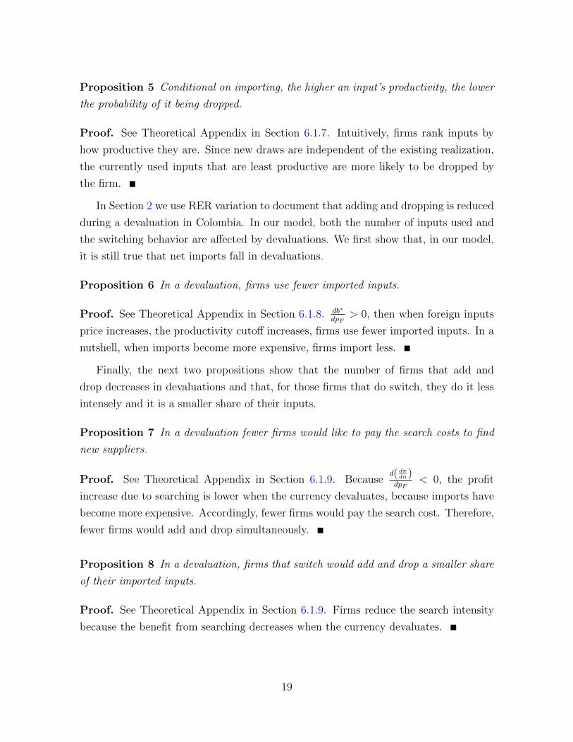
Proposition 5 Conditional on importing, the higher an input’s productivity, the lower

the probability of it being dropped.

Proof. See Theoretical Appendix in Section 6.1.7. Intuitively, firms rank inputs by

how productive they are. Since new draws are independent of the existing realization,

the currently used inputs that are least productive are more likely to be dropped by

the firm.

In Section 2 we use RER variation to document that adding and dropping is reduced

during a devaluation in Colombia. In our model, both the number of inputs used and

the switching behavior are affected by devaluations. We first show that, in our model,

it is still true that net imports fall in devaluations.

Proposition 6 In a devaluation, firms use fewer imported inputs.

Proof. See Theoretical Appendix in Section 6.1.8. db∗

dpF> 0, then when foreign inputs

price increases, the productivity cutoff increases, firms use fewer imported inputs. In a

nutshell, when imports become more expensive, firms import less.

Finally, the next two propositions show that the number of firms that add and

drop decreases in devaluations and that, for those firms that do switch, they do it less

intensely and it is a smaller share of their inputs.

Proposition 7 In a devaluation fewer firms would like to pay the search costs to find

new suppliers.

Proof. See Theoretical Appendix in Section 6.1.9. Becaused( dπdn)dpF

< 0, the profit

increase due to searching is lower when the currency devaluates, because imports have

become more expensive. Accordingly, fewer firms would pay the search cost. Therefore,

fewer firms would add and drop simultaneously.

Proposition 8 In a devaluation, firms that switch would add and drop a smaller share

of their imported inputs.

Proof. See Theoretical Appendix in Section 6.1.9. Firms reduce the search intensity

because the benefit from searching decreases when the currency devaluates.

19

4 Evidence On Firms’ Import Switching Behavior

In this section, we use firm-level data to provide further evidence on firms’ imported

input switching behavior. Our findings are consistent with the model’s predictions.

More precisely, we show regressions that are associated with the propositions in Sec-

tion 3. All of the results in this section are robust to an export switching dummy25,

exporter dummy and share of export value in total sales. Additional robustness checks

are considered by adding a dummy for the first year of importing, to control for the

partial year effects, as in Bernard et al. (2014). In this section, whenever we run a

dynamic panel data regression or include the RER as explanatory variable, the results

are obtained in first differences26.

We start with a specification relating firms’ import behavior to their lagged sales,

a proxy for productivity, and the RER. Results shown in Table 1 are obtained from

running,

Importsit = α + γi + β1RERt + β2Salesit−1 + ωit

where the variable Importsit is either import value or the number of different inputs

imported by firm i at time t. Unless otherwise specified, all variables are in logs through-

out the section. Two results are worth highlighting in this table. First, as firms become

larger, they import more (Proposition 1). Second, both import value and the number

of imported varieties fall when the RER goes down (Proposition 6). Essentially, both

results confirm the findings of the abundant, previous literature.

25If a firm does not export we set the export switching dummy equal to zero.26This makes age, the proxy for the accumulated known supplier mass, drop in some specifications.

20

(1) (2) (3) (4)

VARIABLES Import Value Import Value Import Number Import Number

RER 1.285*** 1.253*** 0.456*** 0.436***

(19.81) (19.34) (11.63) (11.10)

Lagged Sales 0.154*** 0.0992***

(7.208) (8.633)

Constant -0.00676 -0.00896 -0.0138*** -0.0152***

(-1.102) (-1.457) (-3.777) (-4.161)

Observations 35,254 35,254 35,254 35,254

R-squared 0.011 0.013 0.004 0.007

Number of Firms 5,243 5,243 5,243 5,243

First Differences Yes Yes Yes Yes

Robust z-statistics in parentheses

*** p<0.01, ** p<0.05, * p<0.1

Table 1: Value and number of imported inputs and RER.

We now turn to the predictions most closely related to the mechanism in our model.

Import Switching and Age – In the next two tables, we study the dynamic implica-

tions of the model with respect to age (Proposition 3). Both regressions use the same

independent variables. We run

Importsit = αt + γi + β1Ageit + β2Age2it + β3Salesit−1 + εit

where Importsit is either imported inputs or the switching intensity, by firm i at time

t, and Ageit is the number of years firm i has been importing inputs.

In our model, whenever firms choose to search for suppliers, they will accumulate im-

ported inputs and suppliers over time. This implies that older firms use more imported

inputs. The regression in Table 2 has the number of imported inputs as dependent vari-

able, and shows that the prediction of the model is in line with the data: the coefficient

on Age is positive and the quadratic term implies that older firms increase the number

of foreign inputs at a decreasing rate.

21

(1) (2)

VARIABLES Import Number Import Number

Age 0.0656*** 0.0488***

(8.662) (6.458)

Age2 -0.00130** -0.000615

(-2.558) (-1.232)

Lagged Sales 0.214***

(12.26)

Constant 0.952*** -2.246***

(21.23) (-8.511)

Observations 15,153 15,153

R-squared 0.794 0.799

Firm FE Yes Yes

Time FE Yes Yes

Robust t-statistics in parentheses

*** p<0.01, ** p<0.05, * p<0.1

Table 2: Number of products and age.

In the next table we consider another data counterpart of Proposition 3: over time,

it is increasingly difficult to find better foreign suppliers. As firms have spent more

time searching, the value of switching becomes smaller. This is confirmed in Table 3

where age has a negative effect on our switching measures. Further, since older firms

are larger, this also emphasizes that our results are not driven by firms with more

inputs adding and dropping more. The table also shows that conditional on adding and

dropping products, larger firms switch more, in terms of value and number of varieties,

but they switch a smaller share of their inputs, as in Figure 2 27 28.

27 We run a linear probability model, and find larger firms are more likely to add and drop, whichis consistent with the model.

28 At this point it is worth highlighting that at least three pieces of evidence in our empirical resultssuggest switching is not simply due to idiosyncratic input shocks. First, that firms over time use moreinputs. Second, that the share of switching in total imports decreases over time. Third, input dropprobability is negatively related to firm size.

22

(1) (2) (3) (4)

VARIABLES Add and Drop Add and Drop Add and Drop Add and Drop

Value Value Share Number Number Share

RER 1.375*** 1.050*** 0.227*** 0.355***

(7.799) (5.159) (2.655) (4.335)

Age -0.0783*** -0.178*** -0.0126 -0.0774***

(-3.168) (-6.200) (-1.070) (-6.896)

Age2 0.00561*** 0.00580*** 0.00241*** 0.00286***

(3.494) (3.197) (2.622) (4.028)

Lagged Sales 0.298*** -0.266*** 0.137*** -0.0695***

(5.946) (-4.987) (6.248) (-3.557)

Constant 6.462*** 4.018*** -0.155 1.440***

(8.397) (4.868) (-0.458) (4.776)

Observations 6,411 6,411 6,411 6,411

R-squared 0.691 0.679 0.777 0.613

Firm FE Yes Yes Yes Yes

Robust t-statistics in parentheses

*** p<0.01, ** p<0.05, * p<0.1

Table 3: Switching over time.

Input drop – The model also makes predictions at the input-firm level (Proposition

5). We use within-firm variation to show that the likelihood of dropping an input is

related to it’s productivity. In our model, searching allows for the use of more productive

varieties over time. If the productivity draw of a purchased input is large, the firm will

use relatively more of it, and it will be more difficult to find an even better input in

the future; hence, such an imported input will be less likely to be dropped. To test this

hypothesis, we run,

DummyInputDropijt = αt + γi + β1ImportedInputSizeijt−1 + β2Salesit−1 + εijt

where DummyInputDropijt is a dummy for whether input j was dropped or not, where

a drop has been coded as 1. ImportedInputSizeijt is either the imported value of input j

by firm i or the share of the input in total inputs. We show the robustness of this finding

to several choices of specification. Table 4 shows the results, which are in accordance

with the theory: a larger import value for an intermediate is associated with a lower

23

likelihood of it getting dropped29.

(1) (2) (3) (4) (5)

VARIABLES Input Drop Input Drop Input Drop Input Drop Input Drop

Dummy Dummy Dummy Dummy Dummy

Input share -0.0625*** -0.0628***

(-362.7) (-364.5)

Input size -0.0640*** -0.0640***

(-369.3) (-369.1)

Lagged Sales -0.00968*** -0.0361*** -0.00320***

(-7.685) (-30.70) (-2.745)

Constant -0.0824*** 0.860*** 0.494*** 0.554*** 0.917***

(-34.50) (323.7) (22.07) (26.52) (44.16)

Observations 802,704 802,704 802,704 802,704 802,704

R-squared 0.237 0.240 0.119 0.238 0.240

Firm FE Yes Yes Yes Yes Yes

Time FE Yes Yes Yes Yes Yes

Product FE No No No No No

Robust t-statistics in parentheses

*** p<0.01, ** p<0.05, * p<0.1

Table 4: Imported Input Dropping Relation to it’s Productivity.

Import Switching and Import Price – Next, we test the relation between switching

and import prices. In our model, fewer firms engage in switching during a devaluation

(Proposition 7). We run a linear probability model,

DummyAddandDropit = γi + β1Salesit−1 + β2RERt + εit

where DummyAddandDropit is a dummy that takes a value of one if firm i both adds

and drops imports, simultaneously, between t− 1 and t, and zero otherwise. Results in

Table 5 show that fewer firms simultaneous add and drop varieties when the RER goes

down, i.e., during a devaluation. Table 3 have shown that firms switch less intensively

when the RER goes down (Proposition 8). In light of our model, we interpret it as

firms reducing their reorganizing activities as a consequence of import prices going up.

29Note, that our result according to which larger firms are more likely to drop an input, see columns3-5, on Table 4, cannot be explained by a model with idiosyncratic shocks to inputs.

24

(1)

VARIABLES Add and Drop

Dummy

Lagged Sales 0.0564***

(7.091)

RER 0.138***

(4.939)

Constant -0.0115***

(-4.424)

Observations 32,796

R-squared 0.003

Number of Firms 4,651

First Differences Yes

Robust z-statistics in parentheses

*** p<0.01, ** p<0.05, * p<0.1

Table 5: Import Switching LPM and RER.

Import Switching and Growth – One of the unique predictions of our model states

that the gross change in inputs matters for firms’ profit growth. In particular, firms that

do pay the fixed cost of switching engage in adding and dropping which in turn improves

their productivity and sales (Proposition 4). To derive the appropriate regressions to

run, we use the model to express sales as a function of the marginal cost, Salest =

k (λ(bt))1−ρ, where k is a constant. Taking the log of the ratio of sales between two

consecutive periods, we obtain

Log(Salest)− Log(Salest−1) = (1− ρ)Log

(λ(bt)

λ(bt−1)

)(8)

Equation (8) shows that the change in log sales is related to the change in the marginal

cost of the firm which is, in turn, a function of the optimal switching activity. In

particular, the optimal policy of a firm depends on it’s state variables A and n, which

we proxy by lagged sales, and age in the import market, as well as on the aggregate

state, the RER. Accordingly, we start by regressing sales changes on switching using

OLS, and eventually, we use these arguments to motivate an instrument. We run,

Salesit − Salesit−1 = αt + γi + β1InputSwitchit−1 + β2Salesit−1 + β3Ageit−1 + εit

25

where InputSwitchit can be either the gross change in value (or numbers) or a switching

dummy, between t− 1 and t. Sales, switching values or numbers are in logs.

(1) (2) (3)

VARIABLES Sales Change Sales Change Sales Change

Lagged Sales -1.071*** -1.078*** -1.078***

(-67.18) (-67.18) (-67.21)

Add and Drop Value 0.00581***

(3.529)

Add and Drop Number 0.0353***

(3.816)

Add and Drop 0.0278***

(5.274)

Constant -0.00581*** -0.00580*** -0.00565***

(-2.688) (-2.682) (-2.617)

Observations 27,778 27,778 32,490

R-squared 0.509 0.510 0.505

Number of Firms 4,208 4,208 4,594

First Diff Yes Yes Yes

Robust z-statistics in parentheses *** p<0.01, ** p<0.05, * p<0.1

Table 6: Productivity Growth And Gross Import Change.

In Table 6 we obtain results consistent with the prediction. Notice how the switch-

ing dummy is associated with growth in sales. Also, consistent with our model, the

regression shows that gross changes, for both the value and number of varieties, are

positively associated with changes in sales. However, these results could be due to

reverse causality. For example, firms that grow more could also be reorganizing their

production and hence switching more. More generally, it could be the result of a spuri-

ous correlation between growth and switching, so in order to deal with reverse causality,

we instrument gross switching with the RER30 which, as predicted by the theory, are

positively related: When the RER is high there is more switching because the net gain

30As we show in Section 2, RER movements provide variation in imported input prices, and periodswith expensive inputs (low RER) are associated with lower switchings. Our dependent variable, salesgrowth, is arguably independent of the RER level beyond the effect through switching. For robust-ness checks, we control for exporter status, export intensity and export share, industry absorption,competition, and economic crisis. Results from these further robustness check confirmed our findings.

26

from searching is larger. More precisely, we run

1st Stage: InputSwitchit = α1 + γi + δ1RERt + δ2Salesit−1 + δ3Ageit−1 + ωit

2nd Stage: Salesit − Salesit−1 = α2 + γi + β1InputSwitchit−1 + β2Salesit−1 + β3Ageit−1 + εit(9)

The IV results are reported in Table 7. In the first stage, we confirm that both the

import switching dummy and gross switching comove positively with the RER, so our

instrument is relevant31. In the second stage, both the switching dummy and the gross

switching measures are positively associated with changes in sales.

(1) (2) (3) (4) (5) (6)

1st stage 2nd stage 1st stage 2nd stage 1st stage 2nd stage

VARIABLES Add and Drop Sales Add and Drop Sales Add and Drop Sales

Value Change Number Change Dummy Change

RER 1.234*** 0.483*** 0.137***

(5.12) (4.40) (4.90)

Add and Drop Value 0.156***

(4.400)

Add and Drop Number 0.399***

(3.927)

Add and Drop Dummy 1.403***

(4.283)

Lagged Sales 0.279*** -1.124*** 0.157*** -1.128*** 0.0542*** -1.155***

(4.80) (-51.55) (4.53) (-47.69) (6.66) (-42.29)

Constant -0.0111* -0.00217 -0.0849** -0.000609 -0.00946*** 0.00470

(-1.89) (-0.530) (-2.01) (-0.130) (-3.63) (0.976)

Observations 27,778 27,778 27,778 27,778 32,490 32,490

Number of Firms 4,208 4,208 4,208 4,208 4,600 4,600

First Differences Yes Yes Yes Yes Yes Yes

Robust z-statistics in parentheses

*** p<0.01, ** p<0.05, * p<0.1

Table 7: Productivity Growth, Gross Import Change and RER.

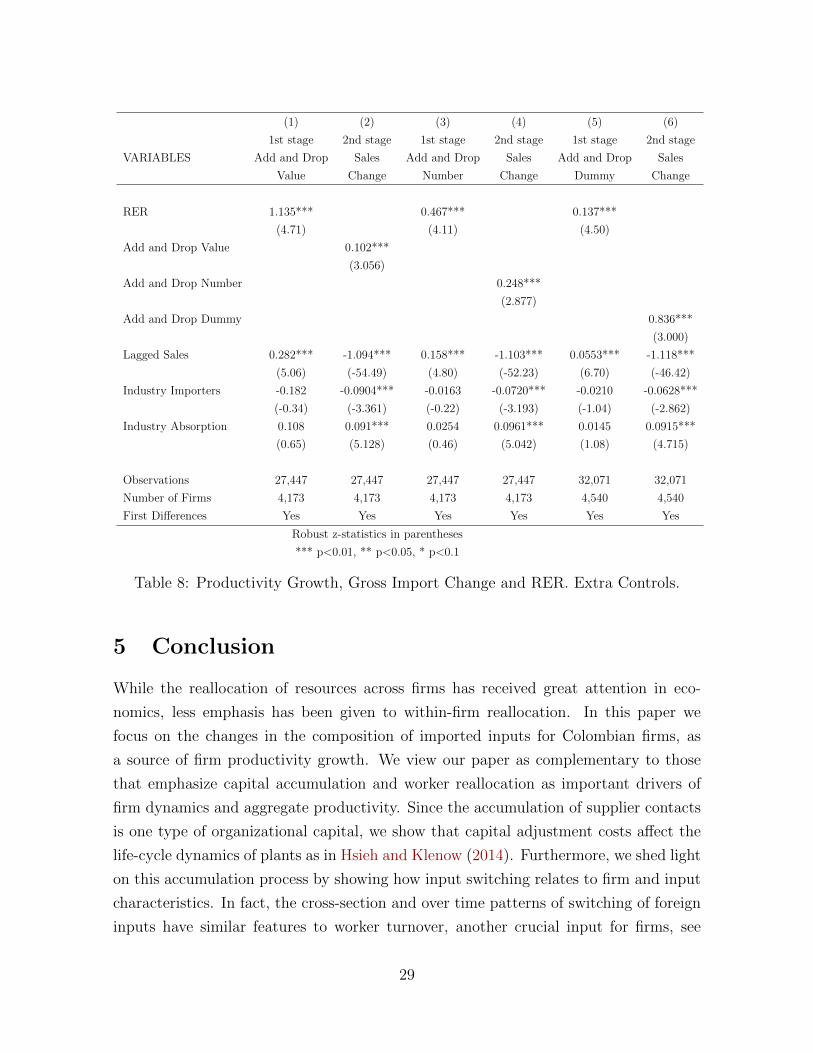
Finally, we address the two main concerns on the IV regression. First, we further

control two other possible channels, demand and competition, in Table 8. Regarding

the demand channel, a devaluation could affect industries’ demand differently. Note

that, while our firm fixed-effects capture the permanent level of firms’ demand, it is still

possible that changes over time in demand across industries could be biasing our results.

31Since we run dynamic panel regressions using first differences, age is dropped.

27

Regarding competition, a devaluation of the Peso makes exporting from the rest of the

world more difficult, which affects competition in Colombia. For example, the reduction

in competition in some industries due to the devaluation could be associated with larger

sales growth for domestic firms and a simultaneous switch in imports. Nevertheless, note

that it is hard to see how these two alternative channels by themselves could generate

less switching and hence be reconciled with the set of facts we report. To control for

the effects of demand and competition, in regression (9) we further include an industry

absorption measure32 and the number of importing firms in each industry33. Results

are in line with our baseline regression34. Second, import switching may be related

to export product churning or to the exporter status more generally. A devaluation

not only makes imports more expensive and import switching less profitable but also

makes exports cheaper. Incumbent exporters could find profitable to change the export

product mix because of the reasons discussed in Bernard et al. (2010) and Timoshenko

(2015). Moreover, cheaper exports could induce entry into the export market, which

may require some adjustment of imported inputs. In both cases, export churning could

alter import demand without productivity gains generated via input search. However,

this channel would generate more instead of less switching during depreciation, and

our results do not change when we control for a time-varying exporter dummy, exports

over sales, and an export product churning dummy. Finally, we also find that further

controlling for the 1999 crisis, by adding a dummy for the relevant observations, does

not alter our results.

32Industry absorption is a measure of domestic consumption and we compute it as industry produc-tion minus exports plus imports.

33For these variables, we define industry at the 2 digit level, which leaves us with 10 industries intotal.

34One might think that switching is simply due to idiosyncratic shocks, but our results are hard toreconcile with a model where imported inputs face iid productivity shocks. In that model, on average,we should not observe productivity gains associated with switching. For larger firms, shocks shouldwash out within a period. For smaller firms they would wash out across periods. However, we findthat larger firms switch more and enjoy greater productivity gains.

28

(1) (2) (3) (4) (5) (6)

1st stage 2nd stage 1st stage 2nd stage 1st stage 2nd stage

VARIABLES Add and Drop Sales Add and Drop Sales Add and Drop Sales

Value Change Number Change Dummy Change

RER 1.135*** 0.467*** 0.137***

(4.71) (4.11) (4.50)

Add and Drop Value 0.102***

(3.056)

Add and Drop Number 0.248***

(2.877)

Add and Drop Dummy 0.836***

(3.000)

Lagged Sales 0.282*** -1.094*** 0.158*** -1.103*** 0.0553*** -1.118***

(5.06) (-54.49) (4.80) (-52.23) (6.70) (-46.42)

Industry Importers -0.182 -0.0904*** -0.0163 -0.0720*** -0.0210 -0.0628***

(-0.34) (-3.361) (-0.22) (-3.193) (-1.04) (-2.862)

Industry Absorption 0.108 0.091*** 0.0254 0.0961*** 0.0145 0.0915***

(0.65) (5.128) (0.46) (5.042) (1.08) (4.715)

Observations 27,447 27,447 27,447 27,447 32,071 32,071

Number of Firms 4,173 4,173 4,173 4,173 4,540 4,540

First Differences Yes Yes Yes Yes Yes Yes

Robust z-statistics in parentheses

*** p<0.01, ** p<0.05, * p<0.1

Table 8: Productivity Growth, Gross Import Change and RER. Extra Controls.

5 Conclusion

While the reallocation of resources across firms has received great attention in eco-

nomics, less emphasis has been given to within-firm reallocation. In this paper we

focus on the changes in the composition of imported inputs for Colombian firms, as

a source of firm productivity growth. We view our paper as complementary to those

that emphasize capital accumulation and worker reallocation as important drivers of

firm dynamics and aggregate productivity. Since the accumulation of supplier contacts

is one type of organizational capital, we show that capital adjustment costs affect the

life-cycle dynamics of plants as in Hsieh and Klenow (2014). Furthermore, we shed light

on this accumulation process by showing how input switching relates to firm and input

characteristics. In fact, the cross-section and over time patterns of switching of foreign

inputs have similar features to worker turnover, another crucial input for firms, see

29

Davis et al. (2012) and Shimer (2012). Analogously, we emphasize that accumulating

imported inputs is a costly activity that takes time, and the efficient use of inputs in-

volves reallocation, as in Pries and Rogerson (2005) studies in the case of workers. Our

proposed mechanism has the potential to be a relevant determinant of aggregate pro-

ductivity growth, given that aggregate reallocation value as share of imports is similar

to the worker reallocation to employment shares.

To understand the mechanisms behind this input reorganization, we introduce dy-

namics through a natural extension of existing models of input choice, by allowing firms

to search for the most productive inputs. The model rationalizes our newly uncovered

facts related to input switching in the data. Our framework not only explains firm

dynamics but can also account for the evidence in Amiti and Konings (2007) among

others, namely, that input tariff reductions are important for productivity growth.

Furthermore, we show evidence that supports the dynamic nature of the process we

highlight, instead of alternative and simpler models. For example, three facts show

that switching is not simply due to random independent shocks to imported inputs.

First, firms’ switching behavior depends on their size and age. Over time, firms use

more inputs and older firms switch less. Second, more productive inputs are less likely

to be dropped. Larger firms are more likely to drop a particular input. Third, imported

input reorganization generates sales growth.

Our model focuses on explaining why firms constantly switch imported inputs, and

how this relates to their age profile and the price of imports. Extending the model to

allow for differential searching intensity across countries would reveal further interesting

dynamic relations between importers and their suppliers. We focus on importers be-

cause it allows us to use detailed data. If we could use matched domestic buyer-supplier

data, it would be particularly relevant to allow firms to search in domestic and foreign

markets simultaneously.

30

6 Online Appendix

6.1 Theoretical appendix

6.1.1 Firms’ Problem

The Lagrangian for the firm problem in the main text is:

L = wL+

∫ 1

0

pHHjdj +

∫b∗pFMbdF (b) + λ

(Y − AL1−αXα

)+ψ

[X − exp

∫ 1

0

lnXjdj

]+

∫b∗χj

[Xj −

[H

σ−1σ

j + (bjMj)σ−1σ

] σσ−1

]dj

Guess that the solution is firms use imported inputs that have productivity larger

than b∗. By the law of large numbers, because there are f (b) fraction of inputs draw

productivity equal b, the price index for intermediate inputs is

pH

∫ 1

0

ln

[1 + I (im)

(bjpHpF

)σ−1] 1

1−σ dj = pH

∫ ∞b∗

ln

[1 +

(bpHpF

)σ−1] 1

1−σ

dF (b) .

And the measure of inputs the firm would use is∫∞b∗f (b) db.

Solving this problem, we get for intermediate good j:

Xj =λαY

pH

[1 +

(bjpHpF

)σ−1] 1

1−σif Mj > 0,

and firm’s unit cost is

λ =1

A

(w

1− α

)1−α

pH exp

∫∞b∗

ln

[1 +

(bpHpF

)σ−1] 1

1−σ

dF (b)

α

α

Define C =(

w1−α

)1−α (pHα

)α, G(b∗) = exp

∫∞b∗

(lnB) f (b) db, andB =

[1 +

(bpHpF

)σ−1] 1σ−1

31

to obtain unit cost as

λ =1

ACG(b∗)−α.

Firm’s total cost is then:

λY +mηF ,

and firm maximizes net profits:

maxY,b∗

(Y

D

)− 1ρ

Y − λ (b∗)Y −m(b∗)ηF , (10)

where m(b∗) =∫∞b∗f (b) db.

The two first order conditions are

Y =

(ρ− 1

ρ

)ρDλ−ρ,

and

−dλdbY − ηmη−1m′F = 0.

This last condition can be written as

−dλdbY − ηmη−1f(b∗)F = −Y C

A(−α)G(b∗)−α−1G′(b∗) + ηmη−1f(b∗)F = 0

αYC

AG(b∗)−α−1G(b∗)(−1) ln

[1 +

(b∗pHpF

)σ−1] 1σ−1

f(b∗) + ηmη−1f(b∗)F = 0,

Using a more compact form, the marginal input satisfies:

αYC

AG(b∗)−α lnB∗ = ηm(b∗)η−1F ,

and using the FOC for Y becomes (2) in the main text:

αD

(ρ− 1

ρ

)ρ(C

A

)1−ρ

G(b∗)α(ρ−1) lnB∗ = ηm(b∗)η−1F . (11)

By rewriting the FOC for b∗, we obtain the next function which will be the basis of

32

our proofs:

αD

(ρ− 1

ρ

)ρ(C

A

)1−ρ

G(b∗)α(ρ−1) lnB∗ − ηm(b∗)η−1F (12)

To check the property of the optimal b∗ we differentiate (12). Also note that the

second order condition is -d(12)f(b∗)db

, which is negative as long as

αD

(ρ− 1

ρ

)ρ(C

A

)1−ρ

G(b∗)α(ρ−1)f(b∗)

α (ρ− 1) (lnB∗)2 f (b∗)−

(pHpF

)σ−1

b∗σ−2[1 +

(b∗ pH

pF

)σ−1]

− η(η − 1)mη−2(f(b∗))2F < 0,

which occurs if η is large enough. In that case the optimal b∗ is unique.

The profit is

π =1

ρ− 1λY −m(b∗)ηF ,

and Y =(ρ−1ρ

)ρDP ρ−1λ−ρ, so

π =1

ρ− 1D

(ρ− 1

ρ

)ρ(C

A

)1−ρ

G(b∗)α(ρ−1) −m(b∗)ηF ,

which using (11) can be written as

π =1

ρ− 1

ηm(b∗)η−1F

α lnB∗−m(b∗)ηF = m(b∗)η−1F

(1

ρ− 1

η

α lnB∗−m(b∗)

). (13)

This is another key equation in our proofs. The effects of A, n, and pF on profits are

through the optimal choice of imported inputs.

6.1.2 Proof of Proposition 1

Proof. From equation (12), d(12)db∗

> 0 and d(12)dA

> 0. So db∗

dA= −

d(12)dAd(12)db∗

< 0.

db∗ndA

< 0,

so when firm productivity increases, the input cutoff decreases and the firm uses more

33

inputs.

6.1.3 Proof of Proposition 2

1. If firms pay the search costs and increase their suppliers, they will drop some

varieties.

Proof. From equation (12), d(12)db∗

> 0, because SOC = −d(12)f(b)db

= −d(12)dbf(b) <

0. And

d(12)

dn= αD

(ρ− 1

ρ

)ρ(C

A

)1−ρ

lnB∗α(ρ− 1)G(b∗)α(ρ−1)−1dG(b∗)

dn−

· · · η(η − 1)m(b∗)η−2Fdm(b∗)

dn=

αD

(ρ− 1

ρ

)ρ(C

A

)1−ρ

lnB∗α(ρ− 1)G(b∗)α(ρ−1)α

∫b∗

lnBdf (b)

dndb−

· · · η(η − 1)m(b∗)η−2F

∫b∗

df (b)

dndb

(14)

Looking at the second term we notice that using more inputs, improves produc-

tivity but increases marginal costs as well. d(12)dn

can be positive or negative. If

η big enough, it is negative. Since db∗

dn= −

d(12)dnd(12)db∗

> 0, searching new suppliers

increases cutoff. Some original inputs should be dropped.

2. If firms search new inputs and increase their suppliers, they will add some vari-

34

eties.

dm(b∗)

dn= −f(b∗)

db∗

dn+

∫ ∞b∗

df(b)

dndb = −f(b∗)

[−d(12)dnd(12)db∗

]+

∫ ∞b∗

df(b)

dndb =

f(b∗)αD

(ρ−1ρ

)ρ (CA

)1−ρln(B∗)α(ρ− 1)Gα(ρ−1)

∫∞b∗ ln(B)df(b)

dn db− η(η − 1)mη−2F∫∞b∗

df(b)dn db

−αD(ρ−1ρ

)ρ (CA

)1−ρGα(ρ−1)

[α(ρ− 1)(ln(B∗))2f(b)− Ebσ−2

1+Ebσ−1

]+ η(η − 1)mη−2Ff(b∗)

...

+

∫ ∞b∗

df(b)

dndb =

f(b∗)αD(ρ−1ρ

)ρ (CA

)1−ρln(B∗)α(ρ− 1)Gα(ρ−1)

∫∞b∗ ln(B)df(b)

dn db− η(η − 1)mη−2F∫∞b∗

df(b)dn db

αD(ρ−1ρ

)ρ (CA

)1−ρGα(ρ−1)

[Ebσ−2

1+Ebσ−1 − α(ρ− 1)(ln(B∗))2f(b)]

+ η(η − 1)mη−2Ff(b∗)=

f(b∗) ln(B∗)[α(ρ− 1)

∫∞b∗ (ln(B)− ln(B∗)) df(b)

dn db+ Ebσ−2

1+Ebσ−1

∫∞b∗

df(b)dn db

][

Ebσ−2

1+Ebσ−1 − α(ρ− 1)(ln(B∗))2f(b)] > 0

Some original inputs should be dropped, but the measure of imported inputs

increases. So if firm paid the search cost and increased its suppliers, they add and

drop imported inputs simultaneously.

6.1.4 Proof of Proposition 3

1. Decreasing returns to searching.

Proof. From Section 6.1.3, we know the mass of imports increases over time.

Here we prove the decreasing returns to scale of our search process. First note

that from Section 6.1.5 we have,

dπ

dn= ηm(b∗)η−1F

∫b∗

(lnB

lnB∗− 1

)df (b)

dndb > 0

35

Also note that since

d2π

dn2=∂(dπdn

)∂b∗

db∗

dn+∂(dπdn

)∂n

=

=db∗

dn

[η(η − 1)m(b∗)η−2m′(b∗)F

∫b∗

(lnB

lnB∗− 1

)df (b)

dndb · · ·

+ ηm(b∗)η−1F (−1)

∫b∗

(lnB∗

lnB∗− 1

)df (b)

dndb · · ·

+ ηm(b∗)η−1F

∫b∗

((−1)

lnB 1B∗

(lnB∗)2− 1

)df (b)

dndb

]· · ·

+ ηm(b∗)η−1F

∫b∗

(lnB

lnB∗− 1

)d2f (b)

dn2db

(15)

Since f(b) = θnT (b− 1)−θ−1 exp(−nT (b− 1)−θ

), then

df (b)

dn= θT (b− 1)−θ−1 exp

(−nT (b− 1)−θ

(1− aT (b− 1)−θ

))which is positive for large b and so

d2f (b)

dn2= 2θT (b− 1)−θ−1 exp

(−nT (b− 1)−θ

(1− nT (b− 1)−θ

)) (−T (b− 1)−θ

)< 0

Using these last two results, equation (15) has the first term negative, since

m′(b) < 0, the second is zero, and the third is negative, while the fourth is nega-

tive. The total effect is that profit increases at a decreasing rate with number of

suppliers.

2. Older firms that have more suppliers have a lower search intensity.

When a firm search, the search intensity satisfies:

dπ (n′, A)

dn′= φ (n′ − n)

γ−1 − βφ (n′′ − n′)γ−1(16)

We have proved that the left hand side is decreasing with n′. The right hand side

increases with n′, hence the equation pins down the optimal searching intensity.

Older firms have a larger n as they accumulate suppliers over time, which shift

the RHS down, and older firms have a lower search intensity n′ − n.

The decreasing return to scale of searching and the convex searching cost make

36

older firms search less intensively, hence they add and drop a smaller fraction of

their imported inputs.

6.1.5 Proof of Proposition 4

1. A larger measure of input suppliers increases profits.

Proof.

dπ

dn=∂π

∂b∗∂b∗

∂n+∂π

∂n=∂π

∂n

∣∣∣∣b∗n

=

αD

(ρ− 1

ρ

)ρ(C

A

)1−ρ

G(b∗)α(ρ−1)−1dG(b∗)

dn− ηm(b∗)η−1F

dm(b∗)

dn=

αD

(ρ− 1

ρ

)ρ(C

A

)1−ρ

G(b∗)α(ρ−1)

∫b∗

lnBdf (b)

dndb− ηm(b∗)η−1F

∫b∗

df (b)

dndb =

ηm(b∗)η−1F

lnB∗

∫b∗

lnBdf (b)

dndb− ηm(b∗)η−1F

∫b∗

df (b)

dndb =

ηm(b∗)η−1F

∫b∗

(lnB

lnB∗− 1

)df (b)

dndb > 0

where the 3rd equality uses Equation (13), and the 5th uses Equation (11).

2. The increased profit from a larger measure of suppliers is larger for more produc-

tive firms. For this part of the proof start using the intermediate step derived

above,

dπ

dn= αD

(ρ− 1

ρ

)ρ(C

A

)1−ρ

G(b∗)α(ρ−1)

∫b∗

lnBdf (b)

dndb−ηm(b∗)η−1F

∫b∗

df (b)

dndb

Now, take derivatives wrt A,

ddπdn

dA= αD

(ρ− 1

ρ

)ρ(ρ− 1)Aρ−2C1−ρG(b∗)α(ρ−1)

∫b∗

lnBdf (b)

dndb+

db∗

dA

(− η(η − 1)mη−2f(b∗n)F · · ·

− ηmη−1F

(∫b∗n

lnBdfn (b)

dndb

) (pHpF

)σ−1

b∗σ−2n

(lnB∗n)2

[1 +

(b∗n

pHpF

)σ−1]) > 0

37

because the first term is positive and db∗

dA< 0

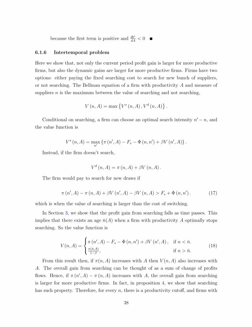
6.1.6 Intertemporal problem

Here we show that, not only the current period profit gain is larger for more productive

firms, but also the dynamic gains are larger for more productive firms. Firms have two

options: either paying the fixed searching cost to search for new bunch of suppliers,

or not searching. The Bellman equation of a firm with productivity A and measure of

suppliers n is the maximum between the value of searching and not searching,

V (n,A) = max{V s (n,A) , V d (n,A)

}.

Conditional on searching, a firm can choose an optimal search intensity n′− n, and

the value function is

V s (n,A) = maxn′{π (n′, A)− Fs − Φ (n, n′) + βV (n′, A)} .

Instead, if the firm doesn’t search,

V d (n,A) = π (n,A) + βV (n,A) .

The firm would pay to search for new draws if

π (n′, A)− π (n,A) + βV (n′, A)− βV (n,A) > Fs + Φ (n, n′) . (17)

which is when the value of searching is larger than the cost of switching.

In Section 3, we show that the profit gain from searching falls as time passes. This

implies that there exists an age n(A) when a firm with productivity A optimally stops

searching. So the value function is

V (n,A) =

π (n′, A)− Fs − Φ (n, n′) + βV (n′, A) , if n < n.

π(n,A)1−β , if n > n.

(18)

From this result then, if π(n,A) increases with A then V (n,A) also increases with

A. The overall gain from searching can be thought of as a sum of change of profits

flows. Hence, if π (n′, A) − π (n,A) increases with A, the overall gain from searching

is larger for more productive firms. In fact, in proposition 4, we show that searching

has such property. Therefore, for every n, there is a productivity cutoff, and firms with

38

productivity above the threshold search. Also, for all cohorts, we can determine what

firms will search at all and if so until what age.

6.1.7 Proof of Proposition 5

Proof. Because draws are independent, the probability of dropping a product with

productivity b is 1− F (b).

6.1.8 Proof of Proposition 6

Proof. From equation 12, d(12)db∗

> 0,. We also have

d(12)

dpF= αD

(ρ− 1

ρ

)ρ(C

A

)1−ρ

G(b∗)α(ρ−1) · · ·− (b∗pH)σ−1 p−σF

1 +(b∗ pH

pF

)σ−1 − lnB∗α(ρ− 1)

∫b∗

(b∗pH)σ−1 p−σF

1 +(b∗ pH

pF

)σ−1f (b) db

< 0

Since db∗

dpF= −

d(12)dpFd(12)db∗

> 0, then when pF increases, the productivity cutoff increases,

firms use less imported inputs: m(b∗) falls.

6.1.9 Proof of Proposition 7 and Proposition 8

Proof. Equation (17) states the condition under which firms search for new draws.

First we show the marginal profit of a larger measure of suppliers is smaller during

devaluation.

d(dπdn

)dpF

=d(ηm(b∗)η−1F

∫b∗

(lnBlnB∗ − 1

) df(b)dn db

)dpF

=

dηm(b∗)η−1F∫b∗

(lnBlnB∗ − 1

) df(b)dn db

db∗db∗

dpF=−η(η − 1)mη−2f(b∗)F − ηmη−1F

(∫b∗

lnBdf (b)

dndb

) (pHpF

)σ−1b∗σ−2

(lnB∗)2

[1 +

(b∗ pHpF

)σ−1] db∗

dpF< 0,

39

because db∗ndpF

> 0. The marginal profit from more suppliers is lower when the cur-

rency devaluates as imports have become more expensive. From Equation (6), firms’

search intensity decreases. Combining the two forces, the overall gains from searching

decreases. Accordingly, fewer firms would pay the searching cost, and for firms that do

pay the searching cost, they search less intensively.

6.2 Empirical Appendix

6.2.1 Harmonized System Code

There are changes of product classification over time by the Harmonized Commodity

Description and Coding system, which would create variety adding and dropping by

firms. We create a correspondence using the document that specify during 1993-2012,

the date when a Decree was approved, the code that the Decree affected and how it

affected it, and the date when the change was applied.

We look at the most conservative case by defining dropped products as products that

were never bought by the firm again, whereas added products as those that have never

been bought by the firm before. Our algorithm uses the concordance and compares the

varieties in the current quarter with all the previous quarters to find added varieties,

and with all the following quarters to find dropped varieties within each firm.

6.2.2 Data Construction

We use two sources of data, the Annual Manufacturing Survey, AMS, and the import

and export transaction data, DIAN. The AMS is a panel of industrial plants from 1994-

2012. Firms enter in the sample if they produce at least 137 million pesos in 2011, or

71.000 US dollars, or have at least ten employees. Once a firm is included in the sample

it is followed overtime until it goes out of business, regardless whether the inclusion

criteria is satisfied each year. It is collected by the National Statistics Department

DANE. The customs data are administrative records of imports and exports collected

by the customs national authority DIAN. Information includes importing or exporting,

HS code of traded product at ten digits (NANDINA), FOB value. NANDINA codes

use standard HS at 6 digits and complements with 4 digits customized for the Andean

Community of Nations.

Next we report all data steps, from cleaning, merging, to variable creation.

40

1. Data Cleaning:

• Data Source 1: AMS:

– Subcontracted products are excluded from the sales value of the firm.

These are products that are not sold by the firm but rather the firm is

hired to produce them using inputs of the contractor.

– Products with value of 0, 1, 2 or 3 are excluded from the sample.

– The original data is at the plant level. We use information collapsed to

the firm-level.

• Data Source 2: Customs:

– Tax identifiers in the customs database are not completely clean as they

may include a verification code in some cases, or letters in others. Both

are truncated to make them match the AMS data format.

– Exclusions are applied, mainly of temporary imports/exports or for pur-

poses of repair or commercial samples. Our trade aggregate data virtu-

ally equals to the aggregates reported by DANE at their website.

2. Merging: AMS and trade data are matched using the unique tax identifier (NIT)

present in both databases.

3. Variable creation:

• Sales: Firm sales are defined as the sum of sales of all products by a firm in

a given year. Value is deflated using the CPI.

• Import value: is the CIF dollar value of imports declared in administrative

records.

• Export value: is the FOB dollar value of imports declared in administrative

records.

• Exporter: indicator variable taking the value 1 if firm has positive export

value, and 0 otherwise.

• Exports share: exports as fraction of total sales.

• Imports/exports number: is the number of different NANDINA codes for a

given firm. See next for an explanation of NANDINA codes.

41

• Absorption: is the current value of production plus imports minus exports

for an industry at CIIUv2 two digits. Only manufacturing industries are

included.

• Number of importer firms by industry: This is the number of firms in the

trade data for a given industry.

• Creation status for varieties: The status of a firm/variety is determined using

data from imports only. There’s a quarterly and a yearly version. The yearly

one is the one used in the regressions. There are five possible statuses for a

firm in a given year:

– Enter: the firm has never imported in the data sample and it’s the first

year it imports.

– Enter old: the firm didn’t import the previous year but imported in any

other year before the previous one.

– Stay: The firm imports in the previous period and the current one as

well.

– Exit: The firm imported in the previous period, but does not import in

the current year nor it imports in the rest of the future years.

– Exit temp: The firm imported in the previous period, didn’t import in

the current one, but import again in a later year of the sample.

• Given the firm status we subdivide the varieties for continuing firms in several

groups:

– Add: the product is new and has never been imported by the firm

– Add old: the product was not imported in the previous year, but has

been imported in some other years before.

– Keep up: The product was imported in the previous period, is also

imported in the current one, and the total import value of it is greater

or equal than in the previous period.

– Keep down: The product was imported in the previous period, is also

used in the current one, and the total used/produced value of it is less

than in the previous period

– Drop: The product was imported in the previous period, but not in the

current one, nor in the future ones.

42

– Drop temp: The product was imported in the previous period, but not

in the current one, but is imported again in the sample.

To classify varieties by their status, several steps are needed, which we de-

scribe here. Imported and exported products are codified using a NAND-

INA code. NANDINA codes are standard Harmonized System at 6 digits,

complemented with additional 4 digits used in the Andean Community of

Nations and in Colombia. This code system is not constant across years.

Some changes are made both at the international HS6 level and at the more

detailed NANDINA level. This changes include reclassifications, opening

of new categories, and closing of old categories. We want to deal with

these changes so we obtain a clean measure of product adding and drop-

ping. Changes do not distribute evenly across years, but occur particularly

in 1996, 2001 and 2007 where modifications were made to the international

Harmonized System.

In sum, the process to determine the status of products involves three steps.

First, using a correspondence of all the products (re)codifications. This

correspondence is available at DANE webpage. Second, creating a file that

determines all past and future codes for a product. In this file each column

has a different combination of past and future codes of a product. Third,

isolating products whose codifications have not changed. For those whose

code that change at any point in time we do the following. For each product

of each firm in a given year, we compare it to the observations in all past

years using the correlative, to decide if a product is indeed newly added

or just the same product with a change in the codification. Similarly, we

compare each product of each firm in a given year, to all products in all

future years, to decide if a product is no longer imported in the future, or is

imported by the firm but with a different code.

• Supplier id’s: data on the supplier of importer lacks a unique numeric iden-

tifier. Accordingly, we use three variables to identify suppliers: country of

origin of the supplier, city of the supplier, and the name of the supplier.

Because different importers may write the name of the supplier in a different

way, we clean the names and use a metric to compare them. We use the Lev-

enshtein Distance, which measures the difference in spelling of two strings.

The most common algorithm is to match them whenever two strings have a

43

distance that is less than a parameter epsilon(10% for example). Because of

the large number of names and spelling possibilities of several countries is

very high we created a different two-step, iterative process.

The first step is to create a new group with the first observation; this first

observation can be thought of as the head of a group. The second step is to

compare the second observation with the head of all the previously existing

groups. If the distance between the two strings is less than a parameter

epsilon, then the new observation is matched to the group with the least

distance calculated. If on the other case all the distances calculated with

all the heads of existing groups are greater than a parameter epsilon, then

a new group is created with this new observation as the head of the new

group. The process is iterated until all the observations are assigned to

previous groups or in their own new group. This simple algorithm gave us

much better results than the more popular method described above.

44

6.2.3 Extra Figures and tables

Sales Add Drop Surviving

Quartile Total Add Drop Net Share Share Importers

1994/1995

1 6.02 4.30 3.38 0.85 0.69 0.58 397

2 7.00 4.64 4.17 0.61 0.67 0.56 543

3 14.20 8.44 6.20 2.68 0.60 0.46 694

4 56.05 27.71 15.92 11.55 0.56 0.36 766

Total 24.57 13.84 8.92 4.95 0.61 0.46 2,400

1998/1999

1 6.29 3.46 4.23 -1.16 0.55 0.53 388

2 7.40 4.20 3.99 -0.05 0.52 0.49 511

3 12.44 5.18 5.79 -0.73 0.45 0.43 646

4 52.37 15.52 15.24 0.22 0.37 0.33 723

Total 22.98 8.82 8.73 -0.32 0.44 0.42 2,268

Table 9: Number Of Different Imported Inputs By Quartile broken down by normalperiod and devaluation.

45

References

G. Alessandria, J. P. Kaboski, and V. Midrigan. Inventories, lumpy trade, and large

devaluations. American Economic Review, 2010. 5

G. Alessandria, H. Choi, and K. J. Ruhl. Trade adjustment dynamics and the welfare

gains from trade. 2014. 4

M. Amiti and J. Konings. Trade liberalization, intermediate inputs, and productivity:

Evidence from indonesia. American Economic Review, 97(5):1611–1638, 2007. 2, 3,

30

C. Arkolakis, T. Papageorgiou, and O. Timoshenko. Firm learning and growth. 2014.

4

A. B. Bernard, S. Redding, and P. K. Schott. Multiple-product firms and product

switching. American Economic Review, 100(1):70–97, 2010. 4, 28

A. B. Bernard, R. Massari, J.-D. Reyes, and D. Taglioni. Exporter dynamics, firm

size and growth, and partial year effects. Working Paper 19865, National Bureau of

Economic Research, 2014. 4, 20

V. M. Carvalho and N. Voigtlander. Input diffusion and the evolution of production

networks. Working Paper 20025, National Bureau of Economic Research, 2014. 4

T. Covert. Experiential and Social Learning in Firms: The Case of Hydraulic Fracturing

in the Bakken Shale. Harvard Thesis, May 2014. 4

J. P. Damijan, J. Konings, and S. Polanec. Import churning and export performance

of multi-product firms. Mimeo University of Ljubljana, 2012. 4

S. J. Davis, R. J. Faberman, and J. Haltiwanger. Labor market flows in the cross section

and over time. Journal of Monetary Economics, 2012. 5, 8, 9, 30

J. Eaton, M. Eslava, D. Jinkins, C. Krizan, and J. Tybout. A search and learning model

of export dynamics. 2014. 4

D. Fitzgerald, S. Haller, and Y. Yedid-Levi. How exporters grow. 2015. 4

46

L. Foster, J. Haltiwanger, and C. Syverson. Reallocation, Firm Turnover, and Efficiency:

Selection on Productivity or Profitability? American Economic Review, 98(1):394–

425, Feb. 2008. 4

P. K. Goldberg, A. K. Khandelwal, N. Pavcnik, and P. Topalova. Imported intermediate

inputs and domestic product growth: Evidence from india. The Quarterly Journal

of Economics, 2010. 2, 3

G. Gopinath and B. Neiman. Trade adjustment and productivity in large crises. Amer-

ican Economic Review, R&R, 2011. 2, 4, 11

L. Halpern, M. Koren, and A. Szeidl. Imported inputs and productivity. American

Economic Review, R&R, 2011. 2, 4, 11

C.-T. Hsieh and P. J. Klenow. The Life Cycle of Plants in India and Mexico. The

Quarterly Journal of Economics, 129(3):1035–1084, May 2014. 4, 29

M. Pries and R. Rogerson. Hiring policies, labor market instituitions, and labor market

flows. Journal of Political Economy, 2005. 5, 30

K. J. Ruhl and J. L. Willis. New exporter dynamics. 2014. 4

R. Shimer. Reassessing the ins and outs of unemployment. Review of Economic Dy-

namics, 15(2):127–148, 2012. 5, 30

Timoshenko. Product switching in a model of learning. Journal of International Eco-

nomics, 95:233–249, 2015. 28

47