how inclusive has growth been in india during 1993/94 …€¦ · · 2015-07-312 how inclusive...

How Inclusive has Growth been in India during 1993/94-2009/10? Implications for XII Plan Strategy

By Sukhadeo Thorat and Amaresh Dubey

1

Disclaimer The views in the publication are those of the authors’ and do not necessarily reflect those of the United Nations Development Programme Copyright © UNDP 2013. All rights reserved. Published in India. Cover Photo © Graham Crouch/UNDP India

2

How Inclusive has Growth been in India during 1993/94-2009/10? Implications for XII Plan Strategy

Sukhadeo Thorat and Amaresh Dubey

Jawaharlal Nehru University, New Delhi 1. Inclusive Growth: XI and XII Plan Periods: India’s Eleventh (2007-2011/12) and the Twelfth Five-Year Plans (2012/13-2017/18) have emerged as being distinct from the earlier Five-Year Plans in so far as these Plans had the goal of inclusiveness at the core of the growth strategy. The main features of the inclusive growth approach under the XI and XII Plans are the following: First, while faster growth is the main goal, the growth of GDP is not treated as an end in itself, but only as a means to an end. Therefore, it focuses on outcomes of increased income, and to realize the desired outcomes, it identifies a particular 'type of growth process’ rather than emphasizing on growth alone for inclusive outcomes. Second, the Plans recognize that the end outcome of growth is reduction in poverty and creation of employment opportunities, improving access to essential services in health, skill and education and other amenities. The third feature is the group focus, which means that pro-poorness would essentially involve outcomes that yield broad-based benefits and ensure equality of opportunity for all, especially the poor, and the poorest among them like the Scheduled Castes (SCs), Scheduled Tribes (STs), other backward castes, minorities and women (11th Plan Vol1, pp. 2). The goal of inclusive growth continued in the XII Plan. The Approach Paper observed:

“Inclusive growth should result in lower incidence of poverty, improvement in health outcomes, universal access to school education, increased access to higher education, including skill development - better opportunities for both wage employment and livelihoods and improvement in provision of basic amenities like water, electricity, roads, sanitation and housing. Particular attention needs to be paid to the needs of the SC, ST and OBC population, women and children as also the minorities and other excluded group.” (Planning Commission, August 2011, pp. 4)

The XI Plan ended in March 2012, and the Approach Paper to the Twelfth Five-Year Plan ‘Faster, Sustainable and More Inclusive Growth’ has been finalized by the Planning Commission. Meanwhile, relevant data, particularly on consumption expenditure and poverty for the most recent years, viz., 2009/10 have also been made public by the National Sample Survey Organisation (NSSO), which provides us with an opportunity to at least investigate the trends in the outcomes for the three years in the XI Plan in terms of inclusiveness and the lessons for the XII Plan strategy for inclusive growth. While ‘Inclusive growth’ has become a strategic pillar of the XI and XII Plans, there are issues on which greater clarity is required, for example, on the definition of inclusive growth, its

3

measures and indicators to monitor the process of inclusive growth at the country and sector level. This paper reviews the current understanding of the concept of inclusive growth, the methods of its measurement, indicators for monitoring the progress in inclusive growth, actual progress during the 1993-2010, particularly during the XI Plan and its implications for the XII Plan. This paper focuses on four interrelated issues. Firstly, it discusses the concept of inclusive growth, drawing mainly from the current literature to bring clarity on the meaning of the term. Secondly, it discusses the issues related to the indicators and measurement of inclusive growth and identifies the indicators for monitoring. Thirdly it provides empirical evidence on the inclusive character of the growth process at the all-India level, since 1993/94 to 2009/10 that includes three years of the XII Five-Year Plan (2006/07 to 2011/12) by defining inclusiveness. Finally, it indicates the implications of the findings for inclusive growth strategy under the XII Plan. The rest of the paper is laid out as follows. Section 2 provides a review of the concept of inclusive growth and its operationalization in quantitative terms. This is followed by description of data sources and methodological issues in section 3. Section 4 has the incidence, change and rate of change of poverty across different socio-religious groups in India by place of residence followed by level, change and growth of monthly per capita expenditure of the households at the same level of disaggregation in section 5. In section 6, we report the elasticity of poverty reduction. Levels and changes in inequality and its impact on change in poverty incidence is examined in section 7. Section 8 summarizes the main findings and discusses its implications for the XII Plan strategy. 2. Pro-poor and Inclusive Growth: Concept and Measurement 2.1 Definition of Inclusive Growth The concept of inclusive growth has been discussed in the recent literature quite extensively.1 Inclusive growth pre-supposes positive increase in income and also non-income dimensions. However, not all growth scenarios are necessarily inclusive. Therefore, there is a need to characterize the inclusiveness of growth as there are several researchers who have tried to separate out the growth process that are inclusive from those that are not.2 It is argued that inclusive growth should be broad-based in the sense that it benefits everyone in the society, including the poor, the near-poor, middle income groups, and even the rich. In the extreme, one could argue that inclusive growth must benefit everyone (Klasen, 2010). Pro-poor growth thus becomes a component of inclusive growth, in which the focus of outcomes is on the poor. Some researchers have gone beyond the income outcome to bring in non-income factors or processes (in the definition of inclusive growth) along with positive changes in income that enable the poor to actively participate in economic activities and benefit from growth. Viewed in this way, this definition signals a

1 For an excellent summary of various concepts of inclusive growth, see Klasen (2010).

2 See Klasen (2010).

4

clear departure from the ‘trickle-down development’ notion of the 1950s and the 1960s that meant a gradual top-down flow from the rich to the poor. Pro-poor growth brings the goal of poverty reduction at the core of the growth strategy, and essentially prescribes substantial income gains from growth in favour of the poor. However, while there is agreement among the researchers about the pro-poor bias in the income distribution, there are, however, considerable differences on the relative extent to which benefits from growth need to benefit the poor to make it inclusive. Discussions in the recent past on pro-poor growth have dealt with the relative increase in the income between poor and non- poor (Grinspun, 2009).3 It is argued that ‘pro-poor growth’ is the positive increase in the mean income that results in "any" decline in poverty, irrespective of the extent of increase in mean income of the poor (Ravallian, 2004). However, some scholars point out the limitation of this measure. According to them, pro-poor growth would encompass a vast majority of growth episodes so long as poverty decreases as most often economic growth does lead to reduction in poverty. Kakwani (2004) in turn proposes that for growth to be pro-poor, the proportionate increase in mean income of the poor should exceed that of the non-poor. With this, the focus of the debate shifted to the extent to which the growth process led to income gains for the poor and non-poor. As a result, the criterion to measure the pro-poorness of growth witnessed further refinements. It is suggested that while the true test of ‘pro-poorness of growth’ is the existence of a policy bias in favour of the poor (resulting in the relatively higher increase in their mean income), increase also needs to be with reference to the country’s past record of poverty reduction and the definition of ‘pro-poor growth,’ which is the process of growth that reduces poverty more than it does in the past benchmark (Osmani, 2005). White proposed three criteria for pro-poor growth, viz., the share of the poor in income exceeds their existing share, their share in incremental income surpasses their share in population, and the share of the poor in incremental income exceeds by some international norm (Grinspun, 2009). Klasen (2010) brought an added dimension by focussing more on the processes that enable inclusiveness and suggested the inclusion of the "non-discriminatory and disadvantage reducing participation" as a necessary condition for growth to be inclusive. Klasen (2010) summarized the concept of inclusive growth (which also includes pro-poor growth as its subset) in terms of both processes and outcomes:

a) Positive per capita income growth rates b) Income growth rates for disadvantaged groups, viz., income poor, ethnic minorities,

women, backward regions, and rural areas are as high as the growth rates for per capita income, indicating that such groups have been able to participate in the growth process at least proportionately, and hence growth has been non-discriminatory

c) Expansion of non-income dimensions of wellbeing that exceed the average rate for disadvantaged groups. Non-income dimensions include achievements in schooling, survival rates, nutritional status, access to transport, communication and household

3 See (Grinspun, 2009) for an excellent summary of the different measurements.

5

services (water, electricity). This would ensure that income growth has been disadvantage reducing.

To sum up, researchers have suggested alternative criterion, which is that growth reduces poverty, increased income benefits the poor more than the non-poor proportionately, it benefits the very poor and not just the poor, and that poverty reduction in the current period is higher than the past benchmark such that the current share of the poor in incremental income exceeds their share in the past, exceeds their population share and meets international norms and that the growth is non-discriminatory and disadvantage reducing. With these criteria, pro-poor growth requires that the pattern of growth should have an in-built bias in its strategies which brings relatively higher gains to the poor from income growth. The growth process itself needs to have elements embedded in it, which will bring substantial incremental income gains for the poor. 2.2 Pro-poor growth, inequality and poverty inter linkages To the extent that the pro-poorness involves reduction in poverty due to gains in incremental income for the poor, the poverty reducing outcome would depend on the trade-off between growth in income and inequality in income distribution. Thus, the key to the definition of pro-poor growth is the joint consideration of growth and the distribution of incremental income. Pro-poor growth is primarily about the distribution of incremental income between lower and upper income groups, such that the proportional increase of the poor exceeds the overall average. It implies that pro-poor growth essentially involves growth with declining inequality in income distribution so that the poor benefit (Rauniyar and Kanbur, 2010). There is rich literature on the inter linkages between growth, inequality and poverty. The first systematic statement on growth and inequality relationship was made by Kuznets in the 1950s when he argued that the long term secular behaviour of inequality follows an inverted U-shaped pattern, with inequality first increasing during the early stages of growth in developing countries but likely to fall after some time (Kuznets, 1955). Empirical studies that follow Kuznets pioneering work provide evidence that the shape of the inverted U curve varies from country to country, determined by a number of factors such as modernization of traditional small and household non-farm production sectors into high productivity activities, increase in employment, human resource development, role of the state, etc. 4 2.3 Initial high inequality and increasingly inequality matter for pro-poor growth Recent research has led to further insights on the relationship between growth, inequality and poverty. High initial inequalities and increase in inequalities (in the process of growth) in fact matters for speed of poverty reduction. The rate of decline in poverty tends to be less pro-poor in a situation where initial inequality is high compared to a situation where initial inequality is lower, and where inequalities increase rather than decrease with economic growth (Ravallion 2009). Further, certain inequalities are found to be particularly pernicious as they not only generate higher poverty in the present scenario, but also impede future growth and poverty reduction for some excluded groups. Ravallion (2009) identified social 4 See for example Ahluwalia (1976, 1976b); Paukert (1973); Adelman and Morris (1973); Papanek (1978);

Tsakloglou (1988).

6

exclusion, discrimination, restrictions on migration, constraints on human development, lack of access to finance and insurance, corruption as sources of inequality that limit the prospects for economic advancement among certain segments of the population, pushing them into persistent chronic poverty.5 3 Data and Methodology 3.1 Data Unit record data from three quinquennial rounds of consumption expenditure surveys (CES) conducted by the National Sample Survey Organisation (NSSO) have been used for measuring growth, incidence of poverty and inequality. These surveys were conducted during agricultural years 1993-94 (July 1993 to June 1994), 2004-05 (July 2004 to June 2005) and 2009-10 (July 2009 to June 2010) respectively. These rounds are also referred to as the 50th, 61st and 66th rounds of quinquennial surveys respectively. While we have carried out all the analyses at three time points, the discussion in the paper is restricted to the period spanning 1993/94 to 2009/10. The calculations for three time points are reported in Appendix 1. 3.2 Poverty Norms and Price Deflators In this paper, we use poverty lines published by the Planning Commission. These are the poverty lines originally derived by the Task Force (GoI, 1979) and modified by the Expert Group (GOI, 1993)6 for calculating state-level Poverty Lines (PL) by adjusting for price variation across states. For the years 1993-94 and 2004-05, the state-wise poverty lines used in this paper have been taken from GoI (1997, 2007). However, since the submission of the Report of the Expert Group to Review the Methodology for Estimation of Poverty in 2009 (GoI, 2009)7 the Planning Commission has not specified a set of poverty lines for 2009-10.8 Moreover,

5 Among the bad inequalities, the one that is particularly important is social exclusion and discrimination.

Studies have started to recognize the close association with chronic and persistence poverty of social/ethnic/religious groups/women and (social) exclusion and discrimination (Becker, 1957; Loury, 1977; Manski, 1993; Durlauf, 1999). Discrimination hinders the opportunities to access and acquire assets, employment and social needs like education, health and food security schemes and to participate in governance and decision making processes and creates situation that reduces the chances to come out of poverty trap (Braun et al, 2010; Thorat, 2010). Social exclusion aggravates poverty directly by denying the fair access to opportunities channelized through markets and non-market transactions and indirectly by adversely affecting economic growth. However, there is limited empirical work that gives insight as to how social exclusion and discrimination cause more poverty among the excluded and discriminated groups. We have much less knowledge about the process of “exclusion induced poverty”. 6In 2009, Planning Commission accepted the recommendation of the Expert Group (GoI, 2009) that proposed a

new set of poverty lines derived using a very different methodology than used in derivation of poverty line earlier. But the poverty lines given by GoI (2009) extend back only to 1993-94. As the analysis carried out in this paper covers a relatively longer duration, dating back to 1983, for comparability of the estimates, we have to use the old poverty line published by the Planning Commission. It is to be noted that our main concern is with distances rather than levels, therefore, the use of any particular poverty line is not likely to affect these comparisons (Dubey and Gangopadhyay, 1998). 7 This is also known as the Tendulkar Committee Report.

8 Though there have been reports in the press that the Planning Commission has submitted a set of poverty

lines for 2009-10 to the Honourable Supreme Court of India recently, this PL has not been used for research purposes yet.

7

the Expert Group Report (GoI, 2009) does not provide a comparable set of poverty lines for the earlier time period, e.g. 1993-94. Consequently, we have updated the poverty line of 2004-05 as reported in GoI (2007) using the Expert Group methodology (GoI, 1993 (Lakadawala Committee)) using state-wise CPIAL and CPIIW for rural and urban areas respectively. Therefore, the incidence of poverty reported in this paper has been calculated using the "old official poverty line".9 The nominal sector-wise poverty lines for four time points are reported in Appendix table A1. The NSS CES data reports consumption expenditure of the households in nominal rupees. We have converted the nominal Per Capita Expenditure (PCE) at constant (1999-2000) prices. The price deflator that we used to convert the household expenditure at constant prices is implicit price deflator derived from the state-wise poverty line for two sectors separately. This is equivalent to deriving a deflator using state and sector-wise CPIs. The value of deflator at a time point t (t = 1993-94, 2004-05 and 2009-10) is defined as-

20001999

PL

PLDef t

t

where PLt refers to the poverty line at time t (t= 1993-94, 2004-05, 2009-10). Using the above relationship, we could derive only 20 rural and 20 urban price deflators for 20 major states. For the remaining states, the deflators have been adopted from the neighbouring states as in Dubey and Gangopadhyay (1998). The measure of inequality, Gini coefficient, has been calculated after deflating Mean Per Capita Consumption Expenditure (MPCE) by appropriate price indexes. The ratio of expenditure share of the bottom 20 percent of the population have been calculated after adjusting for spatial variation of the prices. 3.3 Economic, Social and Religious Groups and Inclusiveness In this paper, the incidence of poverty and real mean per capita total consumption expenditure (PCTE) in the rural and urban sectors is estimated for economic as well as social and religious groups. The Head Count Ratio (HCR) has been used as a measure of poverty. The economic groups have been identified based on the main source of livelihood of the households. In the rural sector, these include self-employed in agriculture (that is farmers, SEAG), self-employed in non–agriculture (non-farm production and business, SENA), wage labour engaged in agriculture and non-agriculture (AGLA, OTLA). For urban areas, the economic groups include self-employed (SEMP), wage/salaried (RWSE), casual labour (CALA) and other households (with multiple sources of income, OTHE). Among the social groups, the identifiable groups from the data include Scheduled Tribes (STs), Schedule Castes (SCs,) and the Others (OTH, non–SC/ST), and the religious groups include the Hindus, Muslims and Other Religious Minorities (ORM, which includes Christian, Sikhs, Jains and several other religious minorities). 3.4 Measuring pro-poorness of growth

9 It could be mentioned here that the expenditure distribution is log-normal in both rural and urban sectors (as

shown in section 3), therefore, the use of a particular poverty line would not affect the study of temporal changes and spatial variation in the incidence of poverty as shown by Dubey and Gangopadhyay (1998).

8

Pro-poor growth is an outcome wherein poverty reduces (at a higher margin) due to proportionately higher increase in mean income of the poor (bottom 20 percent of the population), facilitated by either no change or minimum increase in income inequality in the process of growth. The increased gains to the poor from increased income is captured by some indicators such as higher growth elasticity, decline in Gini ratio, and higher share of bottom quintile in incremental income relative to the share of the top quintile. Pro-poor growth is, thus, a function of higher growth in mean income, accompanied by higher growth elasticity and a higher share of bottom quintile in the incremental income relative to the top quintile. 3.5 Decomposition of the Incidence of Poverty There is some sort of consensus in the development literature that it is only economic growth that can make sustainable reduction in poverty. However, growth, especially in the non-primary sectors, also has the tendency to be concentrated among the few and accentuate inequality. While summary measures like the Gini coefficient have been used to track changes in the inequality, it is also possible to decompose the changes in the poverty reduction into growth and redistribution components. In this paper, we used Kakwani’s (2004) methodology to decompose the changes in the incidence of poverty.10 Given the limitations of data, we used the income concept of pro-poorness of growth. We study the growth in income (proxied by monthly per-capita expenditure (MPCE)) and its outcome for poverty reduction by looking at some indicators of pro-poorness mentioned above. We study the changes in average monthly per capita expenditure and corresponding changes in poverty incidence and also work out the growth elasticity of reduction of poverty to capture the pro-poorness of growth. To capture the gains from income distribution, we examine how far the pro-poorness of growth has been offset by inequality by decomposing the reduction in poverty into growth and distribution components. 4. Poverty Incidence and Changes in Poverty: 1993-2010 In this section, we have examined the level and changes in the incidence of poverty and the head count ratio (HCR). First, the level and changes in HCR have been examined at the aggregate level and further disaggregated into social and religious groups (SRGs) and economic groups in the rural sector for the period between 1993/94 and 2009/10. After the discussion of level and changes in rural poverty, we examine the incidence and changes in urban poverty for the SRGs and economic groups. The level, change and rate of change in the incidence of poverty (measured as head count ratio, HCR) for the entire population, by sector and socio-religious groups is reported in table 1. 11 4.1. Aggregate and by Social and Religious Groups in the Rural Sector Table 1 shows that in 2009-10, HCR is 30% for SCs while the total poverty incidence is close to 22%. The STs who fall outside the caste system suffer the most with the HCR at 33%. The Muslims with 20.5% HCR are poorer than other religious minorities but much less poor than 10

A detailed note on the methodological issues is provided in Appendix 2. 11

Poverty incidence and its changes at all three time points are reported in Appendices A1 and A2.

9

SCs and STs. This was the social and religious composition of the poor in rural areas of the country that prevailed at the end of the first decade of the 21st century.. Between 1993/94 and 2009/10, rural poverty declined at the annual rate of 2.5%, which is equivalent to 15 percentage points decline (Table 1). An examination of the table suggests that across social groups, the rate of decline in poverty has been much higher for Others (i.e. non-ST/SC) followed by SCs and STs--- the per annum decline being 2.7% for Others and 2.4% for SCs and 2.1% for STs. In case of religious groups, the rural poverty has declined at slightly higher rate for Muslims and other religious minorities (ORM) compared with Hindus--- the per annum decline being 2.4% for Hindus, 3.4% for Muslims and 3.6% for ORM. In absolute terms also, the decline has been much higher for Muslims (24.5 percentage points), followed by ORM (15.4 percentage points) and Hindus (13.8 percentage points) (table 1). Thus, poverty reduction of the Muslims is better than that of the Hindus and ORM.

Table 1: Incidence, Change and Rate of Change (annual) in HCR for SRGs and Sector

Socio-religious groups

Poverty incidence (HCR) in percent

1993-94 2009-10

Rural Urban Total Rural Urban Total

ALL 36.9 32.8 35.9 21.9 20.8 21.6

ST 50.2 42.9 49.6 33.0 28.6 32.5

SC 48.3 49.7 48.6 29.6 32.8 30.3

OTHERS 31.2 29.6 30.7 17.5 18.2 17.7

Hindus 36.5 30.6 35.1 22.7 18.8 21.7

Muslims 45.0 47.7 45.9 20.5 34.3 25.1

OTHER RM 27.1 22.4 25.7 11.7 11.2 11.5

Socio-religious groups

Net change in HCR (percentage point) Rate of change (%, annual)

1993/94-2009/10 1993/94-2009/10


ALL -15.0 -12.0 -14.3 -2.5 -2.3 -2.5

ST -17.2 -14.3 -17.0 -2.1 -2.1 -2.1

SC -18.7 -16.9 -18.3 -2.4 -2.1 -2.4

OTHERS -13.7 -11.4 -13.0 -2.7 -2.4 -2.6

Hindus -13.8 -11.9 -13.5 -2.4 -2.4 -2.4

Muslims -24.5 -13.4 -20.8 -3.4 -1.8 -2.8

OTHER RM -15.4 -11.2 -14.2 -3.6 -3.1 -3.4

Note: Includes OBCs Source: Calculated by the authors' using NSS CES unit record data for the respective years.

4.3. By Livelihood Categories and Socio-Religious Groups In the last section, we analysed changes in poverty by socio-religious groups in the rural sector. In this sub-section, we look at the levels and changes in poverty incidence by livelihood categories at the aggregate level and by socio-religious groups. This will enable us to identify the gainers and losers in poverty reduction by the source of livelihood. The NSS classifies the households into self-employed, wage earners and mixed income sources. Both are further sub-divided into those engaged in farm and non-farm activities – namely self-

10

employed in agriculture (SEAG) and non-agriculture (SENA) and agricultural and non-agricultural wage labour (AGLA and OLAH).

Among these livelihood categories, the farm and non-farm wage labourers are the poorest (tables A4 and A5). In 2009-10, about 35% of farm wage labour households and 26% of non-farm labour households were poor. By comparison, the poverty rate for self-employed in agriculture and non-agriculture was about 17%. So, poverty of farm wage labour was twice that of self-employed farmers. Therefore, for growth to be inclusive and pro-poor, the poverty of the wage labour households needs to be reduced at a faster rate. During the period 1993/94 to 2009/10, the rate of decline in poverty has been relatively higher for the self-employed in agriculture (2.8%) and non-agriculture (2.9%), but less for farm (2.3%) and non-farm wage labour (2.5%). The decline was the least for farm wage labour households (table 2). Thus, self-employed households have done better in poverty reduction than the wage labour households. Among the wage labour households, the non-farm wage labour households perform better than farm labour households. Pro-poor growth requires that the poorest, in this case, farm wage labourers, should benefit in term of poverty reduction. Evidence shows that the poverty of farm wage labour also declined, but in terms of rate of decline, this livelihood group benefited the least.

Table 2: Average Annual Change in HCR by HH Type and SRGs in the Rural Sector (1993/94-2009/10)

SRG ST SC OTHERS HINDU MUSLIMS ORM Total

SENA -2.8 -2.6 -3.1 -2.8 -3.5 -4.0 -2.9

AGLA -1.6 -2.3 -2.4 -2.0 -3.8 -3.3 -2.3

OLAH -2.1 -2.1 -2.7 -2.2 -3.4 -4.9 -2.5

SEAG -2.4 -2.2 -3.1 -2.8 -2.9 -1.4 -2.8

OTHE -2.9 -1.7 -3.8 -2.9 -3.9 -5.3 -3.2

ALL -2.2 -2.4 -2.8 -2.4 -3.4 -3.5 -2.6

Note: As in Table 1. Source: As in Table 1.

Is the pattern different for social and religious groups? We first take the self-employed households, and then discuss the trend in wage labour households. Self-Employed households - During 1993/94 to 2009/10, poverty declined for self- employed farm households of all social and religious groups, but at a lower rate for the SCs, STs compared with others among the social groups (table 2). The reduction in poverty was similar for both Hindus and Muslims as far as poverty of self-employed farmers was concerned. The Others among the social groups and Muslims among the religious groups have experienced greater poverty reduction compared to the rest. All social and religious groups experienced decline in poverty in self-employed non-farm households during 1993/94 and 2009/10. However, the poverty of Muslims and ORM households had declined at a higher rate compared with other households. Others among the social groups and Muslims and ORMs among the religious groups benefited more from the growth in non-farm business sector, compared with SC, ST and Hindu households.

11

Wage labour households:- As pointed out above, wage labour households are the core of the poor and hence speedy decline in their poverty is critical to the overall decline in poverty. We have seen earlier that during 1993/94 to 2009/10, the incidence of poverty of the farm and non-farm wage labour had declined at the lowest rates as compared with the other households. Lower decline in poverty was mainly because of ST wage labour households. For instance, the poverty incidence for ST farm wage labour households declined at 1.61% per annum followed by 2.34% for SC and 2.35% for Other households. Similarly, in the case of non-farm wage labour households, poverty declined at a per annum rate of about 2.06% for STs, 2.09% for SCs compared with 2.75% for Other households. Thus, both in case of farm and non-farm wage labour, the ST and SC households have fallen behind in poverty reduction. In the case of religious groups, the Hindus lagged behind the Muslims and ORM To sum up, following trends emerged at the aggregate level:

a) During the overall period 1993/10, self-employed households have done better than the wage labour households in poverty reduction; and non-farm wage labour have done better than farm wage labour. Thus, economic growth was less pro-poor for wage labour, particularly the farm wage labour. This also means that the growth has been pro-poor for the poor farmer and poor producer/petty business households.

b) Between the two periods, there is substantial improvement in the rate of decline in poverty for all types of households, with a significant edge for other (mixed) households and also improvement for farm wage labourer households in the second period.

Disaggregate by social and religious groups: c) Self-employed - During 1993/10, while all self-employed farmers benefited from

decline in poverty, the SCs, STs benefited less and Others among the social groups and Muslims among the religious groups benefited more.

d) During the same period, all self-employed non-farm households experienced decline in poverty, however Others (among the social groups) and Muslims and other minorities among the religious groups benefited more from the growth in non-farm business sector, compared with the SC, ST and Hindu households. The SCs benefited the least.

e) Wage labour households- In the period 1993/10, farm wage labour poverty had declined at the lowest rate compared with other households. Generally, the rate of decline has been lower for STs and SCs compared with the rest. The others among social groups and Muslims and ORM did better than the rest of the groups.

4.4 Urban poverty Urban poverty incidence is of interest for informed policy for three specific reasons. First, the share of population in urban areas has been steadily increasing and larger proportion of the population now lives in the urban settlements. Secondly, in the longer run, an increasingly larger share of growth and employment has to come from the non-primary sectors. Thirdly, the thrust of reforms has been in the sectors that favoured growth of non-primary sector activities for pushing growth and productivity in the economy. As the growth rate picked up in the post-reform period, incidence and change in poverty in the urban

12

sector would indicate how far the poor have been benefiting from the surging growth in the non-primary sectors. Like in the rural sector, we look at the incidence and changes in poverty in the urban sector. First, the level and changes in HCR have been examined at the aggregate level and disaggregated into social and religious and economic groups for the period between 1993/94 and 2009/10. 4.4.1 Aggregate and by Social and Religious Groups The level of poverty incidence in the urban sector at 20.8 percent in 2009/10 is only marginally lower than that in the rural sector discussed above (table 1). During the earlier years too, urban poverty incidence has been lower than rural poverty incidence but the difference between the incidence of poverty in the two sectors has been relatively larger. During the last 16 years between 1993/94 and 2009/10, urban poverty incidence declined by about 12 percentage points only, that is, at about 2.3% per annum, which is only marginally slower than that in the rural sector (2.5%, table 1). As in case of rural sector, we also calculated the poverty levels for different socio-religious groups in urban sector (table 1). Unlike in the rural areas, where STs have the highest incidence of poverty followed by SCs and the Muslims, the order of incidence of urban poverty is different. The incidence of poverty in urban India has been the highest among the Muslims and SCs in 1993/94 and this ordering is evident in 2009/10 as well. The STs are close enough to these two groups whereas Others among the social groups and ORMs among the religious groups have the lowest poverty incidence at about 11.7% in 2009/10. Another interesting observation is that the ordering of incidence of urban poverty across socio-religious groups has remained almost similar since 1993/94. It is the change in the incidence of poverty across socio-religious groups that presents an interesting picture (table 1). Between 1993/94 and 2009/10, poverty incidence declined by about 17 percentage points among the SCs followed by over 13 percentage points among the Muslims, while in case of STs, the decline has been by over 14 percentage points. Thus, the changes in urban poverty suggest that during 1993/2010, urban poverty declined at 2.3% per annum. It declined at a higher rate for Others among the social groups, while it has been the highest for ORMs among the religious groups (3.1%). For Muslims, the rate of decline has been the slowest at 1.8% per annum. Among the social groups, the rate of decline has been the highest among Others at 2.4% annually, while for SCs and STs, it has been uniform at 2.1%. 4.4.2 By Livelihood categories and socio-religious groups Among the economic categories, in 2009/10, the highest level of poverty incidence is among the casual labour households (table A6), while it is the lowest among households whose main source of livelihood is from regular wages and salary (RWSE). Thus, HCR in the urban sector is lowest among the RWSE households followed by the SEMP and CALA. This ordering has been consistent during earlier time points too.

13

Table A8 shows the incidence of poverty for different socio-religious groups along with household type. Within the CALA households, (which suffer from high incidence of poverty), the STs, Muslims and SCs were the poorest in 2009/10 (table A2). It is rather disheartening to note that the same ordering in incidence of poverty has been in existence since 1993/94. Poverty was also high among the self-employed, it was particularly high among the Muslims (36.2%), SCs (35.5%) and STs (30.0%) in 2009/10 (table A3). Even among the RSWE households, poverty level among the Muslims (21.4%) was the highest in 2009/10, and it has continued to be the highest since 1993/94. The differences in poverty incidence in the urban sector across socio-religious groups as well as across different household types appears to be quite robust in the sense that with minor exceptions, the same ranking is visible for the earlier period. 4.4.3 Changes in poverty by household type When we look at the change in terms of annualized rate of decline in poverty incidence in the urban sector, there are several interesting features from table 3. During 1993/2010, poverty declined at the per annum rate of 2.3% as reported earlier. Table 3: Change in Incidence of Poverty by HH Type and Socio-religious Groups in the Urban Sector

HH Type ST SC OTHERS HINDU MUSLIMS ORM Total

1993/94-2009/10

SEMP -2.6 -2.0 -2.5 -2.6 -1.6 -3.6 -2.4

RWSE -3.3 -3.0 -3.1 -3.2 -2.6 -3.6 -3.0

CALA -0.6 -1.7 -1.9 -1.8 -1.4 -2.2 -1.8

OTHER -1.2 -2.2 -3.5 -3.0 -2.8 -4.3 -3.2

ALL -2.1 -2.1 -2.4 -2.4 -1.8 -3.1 -2.3

Note: As in Table 1. Source: As in Table 1 We can make inter-group comparison for all four household types for 1993/10. In case of self-employed households (SEMP), the slowest rate of reduction has been among the Muslims at 1.6% annually followed by SCs at 2%. In the case of regular salaried households (RWSE), poverty declined at a much faster rate among the STs (3.3%) and ORMs (3.6%), than among Others and Hindus. For the SCs, the rate of decline has been 3.0% and the lowest has been among the Muslims at 2.6%. The poverty for Casual Labour Household (CALA) declined at a relatively lower rate among the STs and the Muslims compared with the ‘rest’. The decline was the lowest among the Muslims (0.6%). Thus, poverty declined at the lowest rate among the Muslims for all categories of the households. 5. Growth in Income: Monthly Per Capita Expenditure After having studied changes in poverty, we examine the levels and changes in the mean income (proxies by household expenditure) by place of residence (rural and urban) over time for the identified socio-religious groups (SRGs) as well economic groups. 5.1 Temporal Change in PCTE: Rural and Urban Figure 1 and 2 below show the distribution and change in the real PCTE (at 1993-94) prices at four time points for rural and urban sectors respectively. Firstly, the distribution is log-

14

normal and there is a discernible shift, though moderate, in the distribution towards the right in both the figures. Secondly, given the nature of the distribution in both the sectors, the use of ‘a particular’ poverty line is not likely to affect changes in poverty incidence over time as pointed out earlier (footnote 8) or comparison of poverty incidence across inter-SRG or economic groups. The scrutiny of the two distributions also seems to suggest that in the rural areas, the change in MPCE between 1993/94 and 2009/10 is moderate at the mode of the distribution. In urban sector though, it is far more pronounced and there seems to be a significant shift to the right compared to the extreme left of the distribution. These two figures indicate that since 1993/94, there has been a rightward shift in the distribution of MPCE. In the subsequent sections, we examine this shift in the distribution at various levels of disaggregation indicated above.

5.2 Level and Change in Real MPCE

1993-94, 0-50, 0.09

1993-94, 50-100, 1.53

1993-94, 100-150, 11.54

1993-94, 150-200, 20.65

1993-94, 200-250, 20.69

1993-94, 250-300, 14.91

1993-94, 300-350, 10.08

1993-94, 350-400, 5.80 1993-94, 400-

450, 4.09 1993-94, 450-500, 2.76

1993-94, 500-550, 1.99

1993-94, 550-600, 1.34

1993-94, 600-650, 1.00

1993-94, 650-700, 0.80

1993-94, 700-750, 0.51

1993-94, 750-800, 0.39

1993-94, 800-850, 0.26 1993-94, 850-

900, 0.24 1993-94, 900-

950, 0.21 1993-94, 950-

1000, 0.18 1993-94, 1000-

1050, 0.14

1993-94, >1050, 0.82

2004-05, 0-50, 0.05

2004-05, 50-100, 0.75

2004-05, 100-150, 7.17

2004-05, 150-200, 17.92

2004-05, 200-250, 19.58

2004-05, 250-300, 16.04

2004-05, 300-350, 11.48

2004-05, 350-400, 7.77 2004-05, 400-

450, 5.09 2004-05, 450-500, 3.61

2004-05, 500-550, 2.48

2004-05, 550-600, 1.67

2004-05, 600-650, 1.20

2004-05, 650-700, 0.93

2004-05, 700-750, 0.81

2004-05, 750-800, 0.58

2004-05, 800-850, 0.43 2004-05, 850-

900, 0.35 2004-05, 900-

950, 0.26 2004-05, 950-

1000, 0.22 2004-05, 1000-

1050, 0.16

2004-05, >1050, 1.44 2009-10, 0-50,

0.01

2009-10, 50-100, 0.66

2009-10, 100-150, 5.47

2009-10, 150-200, 14.26

2009-10, 200-250, 17.97 2009-10, 250-

300, 16.59

2009-10, 300-350, 12.41

2009-10, 350-400, 8.83 2009-10, 400-

450, 5.98 2009-10, 450-500, 4.46 2009-10, 500-

550, 3.05 2009-10, 550-

600, 2.13 2009-10, 600-

650, 1.80 2009-10, 650-

700, 1.28 2009-10, 700-

750, 0.86 2009-10, 750-

800, 0.74 2009-10, 800-

850, 0.49 2009-10, 850-

900, 0.42 2009-10, 900-

950, 0.41 2009-10, 950-

1000, 0.31 2009-10, 1000-

1050, 0.20

2009-10, >1050, 1.67

Pop

ula

tio

n P

rop

ort

ion

(%)

Expenditure Class (PCTE at 1993-94 prices)

Figure 1: Distribution of Population by Expenditure Classes: Rural

1993-94

2004-05

2009-10

1993-94, 0-50, 0.08

1993-94, 50-100, 0.39

1993-94, 100-150, 2.95

1993-94, 150-200, 8.10

1993-94, 200-250, 12.37

1993-94, 250-300, 12.56 1993-94, 300-350,

11.18 1993-94, 350-400, 9.64

1993-94, 400-450, 7.49 1993-94, 450-500,

6.06 1993-94, 500-550, 4.73

1993-94, 550-600, 4.06

1993-94, 600-650, 3.39

1993-94, 650-700, 2.71

1993-94, 700-750, 2.07

1993-94, 750-800, 1.89

1993-94, 800-850, 1.40

1993-94, 850-900, 1.34

1993-94, 900-950, 1.03

1993-94, 950-1000, 0.98

1993-94, 1000-1050, 0.69

1993-94, 1050-1100, 0.66

1993-94, 1100-1150, 0.59

1993-94, 1150-1200, 0.48

1993-94, 1200-1250, 0.33

1993-94, >1250, 2.85

2004-05, 0-50, 0.02

2004-05, 50-100, 0.15

2004-05, 100-150, 2.06

2004-05, 150-200, 6.42

2004-05, 200-250, 9.78

2004-05, 250-300, 10.91 2004-05, 300-350,

9.63 2004-05, 350-400, 8.79 2004-05, 400-450,

7.40 2004-05, 450-500, 6.17 2004-05, 500-550,

5.42 2004-05, 550-600,

4.98 2004-05, 600-650, 3.85

2004-05, 650-700, 3.28

2004-05, 700-750, 2.75

2004-05, 750-800, 2.17

2004-05, 800-850, 2.05

2004-05, 850-900, 1.78

2004-05, 900-950, 1.39

2004-05, 950-1000, 1.17

2004-05, 1000-1050, 1.11

2004-05, 1050-1100, 1.05

2004-05, 1100-1150, 0.70

2004-05, 1150-1200, 0.65

2004-05, 1200-1250, 0.56

2004-05, >1250, 5.74

2009-10, 0-50, 0.01

2009-10, 50-100, 0.14

2009-10, 100-150, 1.96

2009-10, 150-200, 5.29

2009-10, 200-250, 7.86

2009-10, 250-300, 9.04 2009-10, 300-

350, 9.01 2009-10, 350-400, 7.69 2009-10, 400-

450, 7.65 2009-10, 450-500, 6.22 2009-10, 500-

550, 5.20 2009-10, 550-

600, 4.55 2009-10, 600-

650, 4.56 2009-10, 650-700, 3.57 2009-10, 700-

750, 3.38 2009-10, 750-

800, 2.95 2009-10, 800-850, 2.14 2009-10, 850-

900, 2.13 2009-10, 900-

950, 1.69

2009-10, 950-1000, 1.78 2009-10, 1000-

1050, 1.27 2009-10, 1050-

1100, 1.15 2009-10, 1100-

1150, 1.10 2009-10, 1150-

1200, 0.87 2009-10, 1200-

1250, 0.79

2009-10, >1250, 8.01

Pop

ula

tio

n P

rop

ort

ion

(%)

Expenditure Class (PCTE at 1993-94 prices)

Figure 2: Distribution of Population by Expenditure Classes: Urban

1993-94

2004-05

2009-10

15

In this section, we look at the level and annualized growth and variation in the real MPCE (at 1999-2000 prices) at different levels of disaggregation. The levels and changes at three time points are reported in Appendix Tables A4 and A5. 5.2.1 Aggregate and by Socio-Religious Groups In this section, we discuss the changes in income proxied by monthly per capita expenditure (MPCE) in rural areas, reported in table 4. During 1993-94 to 2009-10, the MPCE increased at a per annum rate of 1.5 percent. The per annum rate varies among the groups in a narrow range of 1.3% to 1.8%, except for ORM, whose growth rate is 3.2% per annum. Within the groups, the per annum rate is little less than or equal to the overall average for the STs, SCs and Hindus and higher, although by a small margin, for the Muslims (1.85%).

Table 4: Growth of real MPCE (at 1999-2000 prices)

SRGs

MPCE at Constant (1999/2000) prices Rate of Change of MPCE

1993-94 2009-10 1993/94-2009/10

Rural Urban Total Rural Urban Total Rural Urban Total

ALL 447.6 743.4 521.2 554.6 1029.9 683.2 1.5 2.4 1.9

ST 375.6 615.5 397.1 455.4 919.8 504.6 1.3 3.1 1.7

SC 379.5 557.6 411.2 470.0 724.8 521.2 1.5 1.9 1.7

OTHERS 480.1 779.1 566.1 598.7 1091.0 751.7 1.5 2.5 2.0

Hindus 443.7 761.0 517.8 539.0 1061.1 673.2 1.3 2.5 1.9

Muslims 423.0 568.1 472.6 545.1 757.1 616.2 1.8 2.1 1.9

ORM 560.7 957.9 676.3 848.0 1336.9 1005.5 3.2 2.5 3.0


5.2.2 Livelihood Groups We now look at the growth in MPCE across economic groups. During 1993/94 to 2009/10, the rate of change in MPCE varies across household types, as shown in table 5.

Table 5: Growth of MPCE at Constant (1999-2000) prices by HH Type and SRGs in the Rural Sector

(1993/94 -2009/10)


SENA 2.2 1.3 1.8 1.7 1.5 3.2 1.7

AGLA 1.0 1.3 1.3 1.2 2.4 1.7 1.3

OLAH 0.9 1.0 1.5 0.9 2.2 6.4 1.3

SEAG 1.2 1.4 1.3 1.2 1.4 2.2 1.3

OTHE 1.5 1.4 2.7 2.1 3.5 3.1 2.3

ALL 1.3 1.5 1.6 1.4 1.8 3.1 1.5


Among the five household types, the non-farm self-employed households engaged in non-farm production and business activities show a higher increase in MPCE (1.7%) than the rest,

16

but at a similar rate (around 1.3% per annum). The other notable feature of MPCE growth is that the households whose primary source of livelihood is mixed (Others)12 have experienced the highest per annum increase in MPCE at 2.3% indicating that the households with multiple sources of income have gained more (table 5). In other words, diversification in the income sources is beneficial to the households. 5.2.3 By Social and Religious groups Does this pattern vary across the social and religious groups? We first take the self- employed households, and then discuss the trend in wage labour households. In case of self-employed households, we have seen that during 1993/94 to 2009/10, the self-employed in non-agriculture have done better in the rate of increase in MPCE compared with the rest of the household types. It emerges that STs and Others among social groups have done relatively better in the rate of change in MPCE than the SCs and Muslims of the self-employed household. The differences in the rate of increase in MPCE of self-employed agricultural households across social and religious groups during the overall period 1993-94 to 2009-10 are less (vary within narrow range of 1.2% - 1.4%). In case of wage labour households, during the period 1993/94 to 2009/10, at the aggregate level, the MPCE of farm wage labour households increased at a per annum rate of 1.3%. With the exception of Muslims whose MPCE had increased at a slightly higher rate of 2.4%, there was no substantial difference among the social groups in the per annum rate of increase in MPCE. In the case of non-farm wage labour households, during 1993/94-2009/10, the MPCE increased at a per annum rate of 1.6%. The increase has been lower for the SCs (0.99%) and STs (0.94%) compared with the Muslims (2.2%), ORMs (6.4%) and Others (1.5%). To sum up, during 1993/94 to 2009/10, the MPCE increased at the rate of 1. 5% annually, with less variation among the social groups (which varied in a narrow range of 1.3% to 1.8%). The Muslims enjoy a small edge over others. 5.2.4 Household type by Social Groups: We now study the change in MPCE for socio-religious groups by livelihood. Self-employed: The non-farm self-employed households that showed better performance during 1993/10, also did better in case of the STs and Others among social groups, while the SCs and Muslims lag behind in MPCE growth. The self-employed farmers also showed a positive change for all social groups but with less inter-group differences in the rate of change.

Wage Labour: During the period 1993/94 to 2009/10, MPCE of the farm wage labour households increased at a similar rate for all groups, except for the Muslims whose MPCE increased at a slightly higher rate. For non-farm wage labour households, MPCE increased for all groups, but at a lower rate for the SCs and STs and at a relatively higher rate for the Muslims, ORMs among religious groups and the Others among social groups.

17

5.3. Growth of MPCE in the Urban Sector In the preceding section, we looked at the incidence and rate of change in poverty across SRGs and household types in the urban areas. Two unmistakable points that emerge are that the urban poverty incidence has been marginally lower than the rural poverty incidence, and that there have been large socio-religious group differences. Further, the rate of decline in poverty incidence has been different for different social and religious groups. In this subsection, we discuss the rate of increase in MPCE in the urban sector across the same social and religious groups over a 16-year period. During the overall period, the MPCE in the urban sector grew at a rate of 2.2% per annum, which is significantly higher than that observed in the rural sector. Among the household type categories, the highest growth rate has been experienced by the Other group (3.5%), while for the RWSE, it was 2.8% annually (table 6). The lowest rate of reduction has been among the CALA households at 1.8%. Among social groups, during 1993/10, for the SEMP households, the highest rate of growth was for the STs at 3.0% annually and the lowest has been for the Muslims (1.6%) and the SCs (1.9%). Among the CALA households, Muslims had the highest rate of growth at 2.3%, while STs had the lowest at 1.1% followed by the SCs (1.3%) as evident from table 6. Table 6: Growth of MPCE at constant (1999-2000) prices by HH Type and SRGs in the Urban Sector

(1993/94-2009/10)


SEMP 3.0 1.9 2.3 2.3 1.6 2.7 2.2

RWSE 3.8 2.0 2.9 2.8 2.9 2.5 2.8

CALA 1.1 1.3 2.0 1.7 2.3 1.6 1.8

OTHER 2.8 3.3 3.6 3.4 3.3 3.8 3.5

ALL 3.1 1.9 2.5 2.5 2.1 2.5 2.4


6. Growth, Inequality and Decline in Poverty: Role of Inequality in Poverty Reduction It has been pointed out earlier that growth in general has been quite visible. The analysis in the last two sections suggests that there has been substantial decline in poverty incidence which is accompanied by growth in the MPCE. But how good has the growth been for the poor is mediated by the inequality as all sections of the population do not participate in the growth process equitably. It has been argued in recent times that growth has been "jobless," implying that employment in different sectors did not keep pace with the growth of labour force. Consequently, there is a perception that Indian economic growth has been fostering inequality. In the last section, we examined the growth of MPCE across different socio-religious groups and sectors. The analysis suggests that all SRGs have not benefited equally from the economic growth during 1993/94-2009/10. This, to some extent, explains the differential rates of decline in poverty incidence discussed in section 4.

18

Starting with the pioneering work of Jain and Tendulkar (1990), there have been attempts to examine the reduction in poverty incidence by taking into consideration level of inequality and changes in it. In this section, we also examine this complex relationship. A brief summary of the methodological issues and advances since 1991 and methodology used by us in the paper is given in Appendix 2. 6.1 Level and Change in Inequality In this section, we report and discuss the level and changes in inequality across different socio-religious groups as in the earlier sections. Among several measures of inequality, we report two measures of inequality, viz., ratio of mean expenditure of the lowest and highest quintiles and summary measure of inequality, Gini coefficient at two points, 1993/94 and 2009/10.13 Then we examine how much is the level and changes in the inequality on reduction of poverty by decomposing the changes in poverty incidence into growth and distribution components in the next section.

Table 7: Gini Coefficient by Social Group and Sector

SRGs 1993-94 2009-10


ALL 0.30 0.36 0.35 0.31 0.40 0.37

ST 0.28 0.34 0.30 0.28 0.39 0.32

SC 0.26 0.34 0.30 0.26 0.33 0.29

OTHERS 0.30 0.36 0.35 0.32 0.40 0.38

Hindus 0.29 0.36 0.35 0.30 0.40 0.37

Muslims 0.29 0.32 0.32 0.28 0.38 0.33

ORM 0.33 0.39 0.38 0.40 0.41 0.42


In table 7, summary measure of inequality, the Gini coefficient is reported for all in the rural and urban sectors separately as well as six socio-religious groups--- the STs, SCs, Others among social groups and Hindus, Muslims and all other religious minorities (ORMs) among religious groups. Table 7 shows that the Gini ratio has increased for the population as a whole from 0.35 to 0.37 during 1993/10. While consumption-based inequality measures are fairly stable, they underestimate inequality to some extent. Nonetheless, the Gini coefficient does show about 6% increase over the period covered in this paper. Among social groups, the highest inequality level, as captured by the Gini coefficient, is observed for Others- 0.35 in 1993/94 that increased by about 9% to 0.38 in 2009/10. The figure for STs and SCs has been 0.30 in 1993/94 that increased by 7% to 0.32 in case of the STs but declined by 3% in case of the SCs in 2009/10. Among religious groups, the highest level of inequalities was observed for ORMs at 0.38 and the lowest was observed for the Muslims at 0.32 in 1993/94. For Hindus, it was 0.35. It increased across all religious groups

13

Among the measures of inequality, it is also suggested that one could look at the share of bottom quintile in total expenditure. As we are interested in looking at the changes in inequalities, we believe that the direction of change of inequalities would not be affected.

19

as seen from the table. The increase in the Gini coefficient has been the highest for ORMs (11%) and the lowest for the Muslims (3%) while it was 6% for the Hindus. Coming to the sectoral differences in the Gini coefficient, it is significantly lower in the rural areas compared to the urban areas during both the years. In 1993/94, the urban Gini coefficient was about 20% higher than for the entire rural population. This difference increased to 30% in 2009/10. Similar differences are observed across socio-religious groups over the years. But it is the level and change in the Gini coefficient over two time points across socio-religious groups that is interesting. For the rural sector as a whole, the Gini coefficient was 0.30 that increased by 3% to 0.31. Among social groups, the lowest Gini coefficient was observed among the SCs at 0.26, while for Others it was 0.30 and for STs it was 0.28 in 1993/94. Among religious groups, ORMs had the highest level of inequality (Gini 0.33) while for both Hindus and Muslims, it had been 0.29. In 2009/10, the Gini coefficient remained stagnant for both STs and SCs, however, it increased by about 7% to 0.32 for Others. Among religious groups, the Gini coefficient declined by about 3% to 0.28 for Muslims, while it increased by 3% to 0.31 for Hindus. For the ORMs in rural areas, inequalities increased to 0.40 or by 21%. Thus, the level of inequality shows a decline in case of the SCs among social groups and the Muslims among religious groups, while all others have experienced rise in inequality. As pointed out above, the Gini coefficient in the urban sector had been significantly higher than the rural sector during 1993/94 as well as 2009/10. Among social groups, the Gini coefficient increased for the STs (15%) and Others (11%), while it declined for the SCs by 3%. Among religious groups, the highest increase in the Gini coefficient is observed among the Muslims (19%) and the lowest among the ORMs (5%). In case of Hindus, the increase has been 11%. Thus, in urban areas, not only has the Gini coefficient been higher compared to the rural areas, it has also risen, the highest rise being for the Muslims among religious groups and STs among social groups.

It was pointed out that the Gini coefficient is a very stable summary measure of inequality and does not reflect the changes too clearly. We supplement the inequality measure by comparing ratio of the MPCE between the lowest quintile (0-20%) and the highest (81-100%). Table 8 shows the ratio of MPCE between the lowest and the highest quintiles for rural and urban sectors as well as between different socio-religious groups separately in 1993/94 and 2009/10. As evident from the table, Q1/Q5 in 1993/94 stands at 5.3, which increased to 6.3 in 2009/10 for the rural population. In other words, MPCE of the population in Q5 has been 5.3 times higher than those in Q1 in 1993/94. This has increased 6.3 times in 2009/10 implying that there is an increase in the inequality as far as consumption expenditure of the households is concerned.

Table 8: Ratio of MPCE of Lowest and Highest Quintiles

Year/ SRGs

All ST SC OTHERS Hindu Muslim ORM

Rural

1993-94 5.6 5.9 5.3 5.4 5.4 6.1 5.4

2009-10 6.3 6.2 5.5 6.5 6.4 5.8 7.3

20

Urban

1993-94 5.5 5.2 5.4 5.6 5.6 5.0 6.4

2009-10 6.4 6.4 5.4 6.7 6.5 6.5 7.0


Among socio-religious groups in the rural sector, the ratio has increased for all groups though there are variations. While the Gini coefficient remained stagnant or even declined among the SCs in rural areas, this ratio has increased albeit marginally (from 5.3 in 1993/94 to 5.5 2009/10) among the SCs too. Similar marginal increase is observed among the STs (from 5.9 to 6.3) and Others (from 5.4 to 6.5). Among religious groups, the highest increase is among the ORMs (from 5.4 to 7.3). For the Muslims, it declined from 6.1 to 5.8 during the same period. The Hindus experienced an increase in the ratio from 5.4 to 6.4. The picture in the urban sector is similar to that of the rural sector. There is an increase in the Q5/Q1 MPCE ratio for the sector as a whole. Among social groups, there is no change in the ratio for the SCs but for the STs, it increased from 5.2 in 1993/94 to 6.4 in 2009/10. Among Others too, it increased from 5.6 to 6.7. Among religious groups, the highest increase is observed for the Muslims (from 5.0 in 1993/94 to 6.5 in 2009/10). For the ORMs as well as the Hindus, it has also increased. Thus, compared to the level and changes in the Gini coefficient, the inequalities are much more pronounced when we look at the Q5/Q1 MPCE ratio, which shows the rise in inequalities among the STs and SCs in the rural sector that the Gini coefficient does not capture. This also confirms the decline in inequalities among the Muslims in the rural sector. Clearly, growth in the MPCE observed during 1993/94 and 2009/10, shows that there has been an increase in the inequalities for most of the socio-religious groups. 6.2 Decomposition of Changes in Poverty into Growth and Distribution Effects In section 3 and 4, we examined the decline in poverty and growth in MPCE which appear to be negatively correlated. In the last section, we discussed the level and changes in inequality using the Gini coefficient and the ratio of MPCE of Q5 and Q1. This analysis does indicate that there has been a rise in the inequality across board--- for the entire population, in the rural and urban areas as well as in the different socio-religious groups. How far the rise in inequality (change in the expenditure distribution) has affected the decline in the incidence of poverty is investigated by decomposing the change in poverty between 1993/94 and 2009/10?14 In table 9, we have reported the result of this exercise. Table 9 shows the observed decline in poverty (∆H), expected decline in poverty incidence because of growth in MPCE (had the distribution not changed) and how far the change in the distribution between 1993/94 and 2009/10 has offset the decline in poverty incidence for rural as well as urban sectors. The table shows that in the rural sector, the observed decline in poverty incidence, ∆H, is -14.2 percentage points. The decline could have been 23.8 percentage points had this growth occurred without any change in the distribution. However, because of the change in the

14

We have used exact decomposition method of Kakwani (2003). For details on the discussion of the methodological issues involved see Appendix 2.

21

distribution (i.e. increase in inequality) in the rural areas, the ‘loss’ in the poverty decline is to the tune of 9.6 percentage points. As we have seen above, the rate of growth of MPCE as well as the increase in inequalities has not been uniform across socio-religious groups. This has resulted in a variable decline in poverty incidence as evident from table 9. For example, between 1993/94 and 2009/10, because of growth in the MPCE, the highest level of decline in the level of poverty could have been among the STs, by 36 percentage points, however, due to rise in the inequalities, more than 22 percentage points got offset. Similarly, for the SCs and Others, MPCE growth could have reduced poverty by close to 30 and 26 percentage points respectively. However, due to rise in inequalities, 14.1 percentage points for the SCs and 14.8 percentage points for others got offset. A similar pattern is observed across religious groups too. Although the highest reduction in poverty is observed among the Muslims in the rural areas at 14.9 percentage points, the decline could have been 33.6 percentage points had 18.6 percentage points not been offset by change in distribution. In case of the Hindus and ORMs, we observe similar offsetting effect of change in the distribution as far as decline in poverty is concerned.

Table 9: Decomposition of Change in Poverty Incidence Between 1993-94 and 2009-10 (Growth and Distribution Effects)

Socio-religious Groups

Rural Urban

∆H Growth Effect

Distribution Effect ∆H

Growth Effect

Distribution Effect

All -14.2 -23.8 9.6 -11.4 -26.4 15.0

ST -13.5 -36.0 22.5 -18.6 -27.9 9.4

SC -15.8 -29.9 14.1 -18.7 -29.4 10.7

OTHERS -11.0 -25.8 14.8 -12.6 -22.2 9.6

Hindu -11.2 -25.7 14.4 -14.1 -23.1 9.0

Muslim -14.9 -33.6 18.6 -16.9 -25.5 8.7

ORM -8.3 -18.1 9.8 -12.5 -24.7 12.2

In the urban sector, because of the growth effect, the HCR could have declined by about 26.4 percentage points for all. However, because of distributional changes, 15 percentage points were offset. Among social groups, growth of MPCE could have reduced poverty by about 28 percentage points for the STs, over 29 percentage points for the SCs and by over 22 percentage points for the Others, but 9.4, 10.7 and 9.6 percentage points were offset by the rise in inequalities within these groups. Among religious groups, because of MPCE growth, the highest poverty decline by 25.5 percentage points could have been among the Muslims, however, 8.7 percentage points were lost in poverty decline due to rise in inequality. Similarly, the expected decline for the Hindus has been 23.1 percentage points and for the ORMs 24.7 percentage points, but 9 and 12.2 percentage points were lost due to rise in inequality. Thus, though there are only modest changes in the inequality measure, the Gini Coefficient during this period (table 7 above), the worsening in the distribution seem to be playing a role in decelerating reduction in poverty incidence.

7. Elasticity of Reduction of Poverty and Pro-poorness of the Growth

22

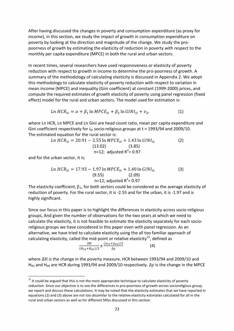
After having discussed the changes in poverty and consumption expenditure (as proxy for income), in this section, we study the impact of growth in consumption expenditure on poverty by looking at the direction and magnitude of the change. We study the pro-poorness of growth by estimating the elasticity of reduction in poverty with respect to the monthly per capita expenditure (MPCE) in both the rural and urban sectors. In recent times, several researchers have used responsiveness or elasticity of poverty reduction with respect to growth in income to determine the pro-poorness of growth. A summary of the methodology of calculating elasticity is discussed in Appendix 2. We adopt this methodology to calculate elasticity of poverty reduction with respect to variation in mean income (MPCE) and inequality (Gini coefficient) at constant (1999-2000) prices, and compute the required estimates of growth elasticity of poverty using panel regression (fixed effect) model for the rural and urban sectors. The model used for estimation is-

(1) where Ln HCR, Ln MPCE and Ln Gini are head count ratio, mean per capita expenditure and Gini coefficient respectively for ith socio-religious groups at t = 1993/94 and 2009/10. The estimated equation for the rural sector is:

(2) (13.02) (3.85)

n=12; adjusted R2= 0.97 and for the urban sector, it is:

(3) (9.55) (2.09)

n=12; adjusted R2= 0.97

The elasticity coefficient, 1, for both sectors could be considered as the average elasticity of reduction of poverty. For the rural sector, it is -2.55 and for the urban, it is -1.97 and is highly significant. Since our focus in this paper is to highlight the differences in elasticity across socio-religious groups, And given the number of observations for the two years at which we need to calculate the elasticity, it is not feasible to estimate the elasticity separately for each socio-religious groups we have considered in this paper even with panel regression. As an alternative, we have tried to calculate elasticity using the all too familiar approach of calculating elasticity, called the mid-point or relative elasticity15, defined as

(4)

where is the change in the poverty measure, HCR between 1993/94 and 2009/10 and H93 and H09 are HCR during 1993/94 and 2009/10 respectively. is the change in the MPCE

15

It could be argued that this is not the most appropriate technique to calculate elasticity of poverty reduction. Since our objective is to see the differences in pro-poorness of growth across socioreligious group, we report and discuss these calculations. It may be noted that the elasticity estimates that we have reported in equations (2) and (3) above are not too dissimilar to the relative elasticity estimates calculated for all in the rural and urban sectors as well as for different SRGs discussed in this section.

23

between 1993/94 and 2009/10 and y93 and y09 are the MPCEs during 1993/94 and 2009/10 respectively. The elasticities calculated using this traditional formula is also referred to as the relative elasticity. Table 10 presents the elasticity of reduction of poverty with respect to growth overall and for social and religious groups. For the rural sector, relative elasticity is - 2.4, which is lower than the estimated elasticity (though similar) reported in equation (2) above.16 If we compare relative elasticities across social groups, the STs have the lowest relative elasticity at -2.2, while Others have the highest at-2.6. The SCs have it at -2.3. Among religious groups, it is the highest among the Muslims (-3.0) and the lowest among ORMs (-2.0), while Hindus have lower (-2.4) than the Muslims. In the urban sector, the relative elasticity is -1.4 which is significantly lower than the estimated elasticity of -1.97. However, relatively elasticity calculation does allow us to see the differences across socio-religious groups. The relative elasticities reported in the table shows that among social groups, the SCs have the highest with -1.6, followed by the Others (-1.4). It is relatively low for the STs and the Muslims at -1.0 and -1.1, respectively.

Table 10: Relative Elasticities of Change in HCR for SRGs by Sector

SRGs 1993/94-2009/10

Rural Urban

ALL -2.4 -1.4

ST -2.2 -1.0

SC -2.3 -1.6

OTHERS -2.6 -1.4

Hindus -2.4 -1.5

Muslims -3.0 -1.1

ORM -2.0 -2.0

Note: As in Table Source: As in Table

7.1 Relative Elasticities for SRG by Household Type: Rural Sector Table 11 reports the elasticity of poverty for economic groups by their social and religious background. We have seen that during 1993/2010, the elasticity was 2.4. The elasticity of poverty was relatively higher for self-employed farmers at -3.0, followed by non-farm self- employed households and non-farm labour households at -2.5 in the second place. The elasticity of poverty reduction is the lowest for the farm wage labour.

Table 11: Relative Elasticities of HRC with respect to MPCE by HH Type and SRGs in the Rural Sector

(1993/94 to 2009/10)


SENA -1.9 -2.7 -2.6 -2.4 -3.5 -2.3 -2.5

AGLA -1.9 -2.4 -2.5 -2.3 -2.7 -3.1 -2.3

OLAH -2.8 -2.7 -2.6 -3.1 -2.5 -1.9 -2.5

16

The magnitude of elasticity discussed in this section is by disregarding the negative sign (-), e.g. though -2.4 > -2.55, by higher elasticity, we mean the latter.

24

SEAG -2.8 -2.1 -3.4 -3.3 -3.1 -0.8 -3.0

OTHE -2.8 -1.5 -2.5 -2.1 -2.1 -3.7 -2.2

ALL -2.2 -2.3 -2.6 -2.4 -2.9 -2.0 -2.4


Looking at the elasticity of poverty reduction for social groups by the household type, we find that the AGLA and OTHE have the lowest elasticity. In case of the self-employed households, elasticity of poverty reduction for the SC farmers is lower than the other SRGs during 1993/2010. The non-farm self-employed households had the highest elasticity of poverty overall. The level was also high for all social and religious groups, except STs during 1993/2010. Thus, during 1993/2010, the elasticity of poverty was relatively high for the self-employed farmers and the non-farm household and the non-farm labour households. The elasticity of poverty was the lowest among the farm wage labour, although it was relatively higher among the non-farm labour. 7.2 Elasticity of Poverty Reduction: Urban Sector During 1993/10, the elasticity of poverty reduction with respect to growth of MPCE in the urban sector, as reported in table 10, has been -1.4, which is lower than that in the rural sector (-2.4). The higher elasticity is observed for the RWSE among socio-religious groups, with the highest being for the SCs (-2.2), while elasticity has been lower for the STs in social groups and the Muslims in the religious groups among the households belonging to the RWSE category.

Table 12: Relative Elasticities of Decline in HCR with respect to MPCE by HH Type and SRGs in the Urban Sector

HH Type ST SC OTHERS HINDU MUSLIMS ORM All

1993/94-2009/10

SEMP -1.4 -1.4 -1.6 -1.7 -1.3 -2.3 -1.5

RWSE -1.5 -2.2 -1.8 -1.8 -1.4 -2.4 -1.8

CALA -0.6 -1.6 -1.3 -1.4 -0.8 -1.9 -1.3

OTHER -0.6 -1.0 -1.7 -1.5 -1.4 -2.3 -1.5

ALL -1.0 -1.6 -1.4 -1.5 -1.1 -2.0 -1.4


The lowest elasticity at -1.3 is observed for the casual labour households among the four household types in the urban sector. Among social groups, the STs (-0.6) and among religious groups, the Muslims (-0.8) have the lowest elasticity. For a large proportion of households belonging to the SEMP, the urban sector ranges from petty traders to highly- qualified professionals. The difference in the elasticity across socio-religious groups in this category to some extent reflects the differences in the skill levels and human capital accumulation. Accordingly, we find lower elasticity among the STs and SCs in the social groups and among the Muslims in the religious groups. Similar is the case with other

25

household type which has multiple sources of income. The differentiation across socio-religious groups is similar to that of the SEMP households.

8. Conclusions and Policy Implication for Pro-poor Growth In this section, we summarize the findings of our analysis and outline its implication for the policy. 8.1 Summary of the Findings and Conclusion In this paper, we examined the changes in incidence of poverty and its relationship with growth during nearly two decades, since the large-scale economic reforms were initiated. One of the consequences of the reforms has been the significantly higher rate of economic growth since early 1990s. How far the growth in income has affected decline in poverty has been widely debated and several studies have concluded that the decade of 1990s has been a ‘lost’ decade as far as decline in poverty is concerned. In this paper, we extend the period of analysis to 2000s and examine the changes in poverty in relation to growth between 1993/94 and 2009/10 and see how far the deterioration in the distribution has affected change in poverty. The analysis is carried out for rural and urban households, by socio-religious affiliation of these households as well as for the economic categories of the households classified by the sources of income of the households. We find that there has been a substantial decline in poverty that could be attributed to sustained average higher growth in income during 1993/94 and 2009/10. However, we also point out that there is evidence of rise in inequalities that has eroded to a large extent the potential of growth to reduce poverty. More significantly, we find that there are substantial differences across socio-religious groups as far as participation in the growth and reduction in poverty is concerned, as indicated by the responsiveness of the poverty to growth of income. In the light of the results on changes in poverty, monthly per capita expenditure and the pro-poorness of the growth by social and economic groups, we indicate the implications for the pro-poor policy. The findings point towards strengthening some well-known existing policies and suggesting some new ones. 8.2 Implications for the Policy: Farm Sector In the agriculture sector, the most poor are small farmers, and farm wage labour. The growth in the agriculture sector has been, by far, more poverty reducing in the rural areas. Relatively high elasticity of poverty “for self employed farmers" implying that agricultural growth has been most poverty reducing compared with any other rural livelihood household category and helped poor small and marginal farmers in reducing their poverty. This is a positive message of agriculture growth and poverty linkages that were established by several researchers (see, for example, Ahluwalia, 1976). Since agricultural growth has poverty reducing potential, there is a need to strengthen and continue the present pattern of growth. This would necessarily involve raising of productivity of small farmers through land development and water resources on small farms, ensuring easy supply of inputs

26

including improved inputs , credit, access to extension services, and above all, the remunerative prices for their products .There is an excellent opportunity for the Government to use the Mahatma Gandhi National Rural Employment Guarantee Scheme for land improvement and development of irrigation and water resources through well irrigation and watershed development and other water harnessing technologies. The land and water resources development of small farms has great potential for productivity enhancement and poverty reduction. While there is a potential to reduce poverty of small farmers, there is, however, a downside to it, which needs to be addressed through policy. In relative terms, agricultural growth lacks the potential to reduce farm wage labourers' poverty in the same measure as it did for small farmers. Distribution of gains from increased farm income seems to be shared unequally by poor farmers and poor farm wage labour households engaged in agriculture. The elasticity of reduction in poverty with respect to MPCE has been much less for farm wage labour compared with self-employed farmers. In fact, it has been the lowest for wage labourers engaged in agriculture. Low pro-poor character of the agricultural growth with respect to farm wage labour explains as to why the farm wage labourers' poverty has declined at the lowest rate compared with any other rural household during 1993/2010. Therefore, policy should make agriculture more ‘pro-farm wage labour’ or more poverty reducing for farm wage labourers. In this, however, the challenge is far more complex. Evidence from farm management studies shows that the employment potential of the farming based on small farm sector is less compared with medium and large farm sector, as the former tends to use more of family labour on their own farm compared with medium and large farms, and thus, less demand for hired wage farm labour (Rudra, Ashok 1982). Given the fact that the bulk of the farm sector is small, it has limitations to meet the employment need of wage labourers. Therefore, till the farm wage labourers are gainfully absorbed in rural non-farm and urban sectors, the only way for these assets-less wage labour households is the present NREGA. Therefore, NREGA needs to be strengthened so that it can serve as a supplementary to farm employment. There was another downside to the poverty reducing agricultural growth during 1993/10. Agricultural growth during this period had been less poverty reducing for poor small farmers from the SCs, as compared with their counterparts from the higher caste Hindus (which include the bulk of the higher castes) and the Muslims. The agricultural growth has also been less poverty reducing for the STs, although they did better than the SC farmers. Thus, agriculture growth has resulted in relatively less gains for the small and marginal farmers from the SC/ST categories than the ‘rest’. This requires development of additional policy measures for the small farmers from SC/ST category. Further, these policy measures would require a supplementary ‘affirmative action agriculture policy for small farmers belonging to the SC and ST categories". However, constrains faced by SC farmers are different from those face by the ST farmers. This indicates that small farmers belonging to the SC category face constrains in raising their income from farming which are specific to them. The studies have shown that the net and gross income per acre of the SC and ST farmers tends to be lower than ‘the rest’. Among other reasons, the lower performance of the SC farmers is linked with lower use of various inputs such as irrigation (particularly private tube- well irrigation), modern implements and other biochemical inputs (Berner, Thorat and Sirohi, 2008). However, part of the reason for the lower use of these inputs is the discriminatory access of

27

SC farmers to various markets selling these requisite inputs such as private tube well irrigation, modern implements and other bio-chemical inputs. The SC farmers also face discrimination in the sale of other products such as vegetables and milk, which in turn, affects their sale and agricultural productivity and profitability. So, caste-based discrimination in accessing these inputs and sale of farm outputs from the village markets is specific to the SCs (Thorat et al 2010). Therefore, to enable farmers from the SC community to access requisite inputs and safeguard them from discrimination, additional measures are required. These would necessarily include policies with respect to credit, irrigation, seeds and sale of farm outputs. Similar policies are required for the ST farmers to address their group specific problems. For example, the Government has developed a procurement policy in government purchase under which 20 percent of its purchase would come from the small and micro enterprises belonging to the SC/ST private entrepreneurs. The extension of this procurement policy to vegetables, fruits, milk and other such commodities where SC farmers face more discrimination will be a good step to overcome constrains faced by the SC/ST small farmers and to promote inclusive agriculture growth, which is the main objective of the 12th Plan. The Government’s proposed procurement policy for some agricultural products from SC small farmers should also be extended to purchases by private industrial sector. In the case of STs, the problems are different. The STs have relatively better access to agricultural land, however, their productivity is rather low. The farmlands operated by tribals are also of low quality. In view of this, it is imperative to develop situation specific agricultural technology that suits the agro-climatic condition. Technology is required not only for the crop sector, but also for forest cultivation, horticulture, grass cultivation for livestock, dairy and other such economic activities. Another downside of agriculture growth during this period was the lowest elasticity of poverty decline for farm wage labour belonging to the ST households in particular. The agricultural growth has been less pro-poor for the farm wage labour from the STs. The SC farm wage labour did better than the STs, but somewhat less than the higher caste and Muslim farm wage labourers. For the higher castes and the Muslims, the growth has been more pro-poor. The employment generating agricultural growth is, therefore, a necessary strategy to make agriculture growth more ‘pro-poor forfarm wage labour,’ which will benefit both SC/ST and the non-SC/ST farm wage labour. However, additional measures in the form of affirmative action policy in employment in rural area are also necessary. Evidence shows that the SC wage labour also faced discrimination in employment in selected agricultural operations and some non-farm activities and jobs, as a result of which, their unemployment rate was higher than their wage labour counterparts from the higher caste. (Thorat, Sadana and Mallick 2010). Therefore, supplementary employment with preference in public employment is necessary. This provides enough justification for the introduction of public employment and the preference for SC/ST wage labour by the Government in the form of employment guarantee. Thus, if we go by the experiences since the early 1990s and 2000s, the inclusive policy for farm sector would need changes such as:

a) Higher growth in agriculture with labour intensive technology

28

b) Focus on small farm sector as it constitutes the bulk of the poor among the farmers. Since agriculture has exhibited features of being pro-poor towards them, accelerated growth in farm output of small farmers will help to reduce poverty among them. The elements of such a ‘small farm pro-poor strategy’ will have to be clearly embedded in the pro-poor agricultural policy that the 12th Plan has proposed

c) Among the small farm segment, the small farmers from the SCs and STs will need special focus as agricultural growth has been less pro-poor for them. This will require an affirmative action policy for the SC/ST farmers to facilitate non- discriminatory access to the input and commodity markets and development of technology suited to agro-climate situation of ST farmers

d) Since the growth has been less pro-poor for farm wage labour, special attention is needed for them through employment enhancing agricultural growth. For the wage labour from SC/ST, strengthening of affirmative action policy in public employment programme is necessary

8.2 Implication for the Policy: Rural non–farm sector Both self-employed producers/business households and non-farm wage labour which constitute two livelihood groups seem to have benefited equally from the growth during the period under consideration. However, the pro-poorness varies across the social and religious groups. In the case of non-farm self-employed households engaged in production and business, the growth has been more poverty reducing for the Muslims, followed by the STs. The private enterprise/business owned by the STs is much less pro-poor. Therefore, it is necessary that the 12th Plan undertakes a serious review of the strategy for tribal enterprises and businesses and incorporates pro-poor element in the strategy. In the case of non-farm wage labour households, we observed less inter-group differences in the pro-poor character of the non-farm growth. 8.2 Implication for the Policy: Urban Sector Among the three livelihood household categories, namely self-employed, regular salaries/wage earner and casual labourer in the urban sector, the growth has been more pro-poor for the regular salaried followed by those in the self-employed and casual wage labour categories. However, in case of the regular salaried, growth has been relatively more poverty reducing for the SCs, followed by the higher castes, the STs and the Muslims. In other words, it has been the least pro-poor for the Muslims. Thus, it is important to promote regular salaried employment for both the Muslims and the STs residing in the urban areas. While expansion in employment in the urban sector should continue, there is also a need to enhance the employability through promotion of education and skills among the poor households from the SCs, STs and the Muslims. In addition to this, the policy should also address the issue of possible discrimination in employment in the private sector (Thorat and Attewell, 2010). There is empirical evidence that suggests that the reservation policy for the public sector has benefited the SCs and STs, hence higher elasticity of poverty reduction. In the case of self-employed, the higher caste benefits more than the other social and religious groups, namely the STs, SCs and the Muslims. Again, although the elasticity is the same for these three groups, it is particularly low for the Muslims. Therefore, it is important

29

that in the 12th Plan, the policy is revised in favour of the small and micro private enterprises owned by the Muslims, SCs and STs. As mentioned earlier, the Government has developed a policy under which 20 percent of its purchase from the small and micro enterprises would come from the private enterprises owned by the SCs and STs. It must be mentioned that almost 52% of the Muslim households are engaged in self-employed enterprises and businesses. Therefore, a policy to increase the productivity of the macro and small enterprises operated by the Muslims needs to be developed. The policy for modernization of the small and macro enterprises will go a long way in reducing the poverty of this group. Lastly, the casual wage labour households, who are the most poor among the four livelihood categories, have recorded the lowest decline in poverty and the lowest elasticity compared to the rest. This was particularly in the case of the STs and the Muslims. Increasing the employability through vocational and skill education is the only way of pulling them out from chronic poverty. This, too, calls for a public employment programme in urban areas, similar to that in rural areas.

30

References

Adelman I and C. T. Morris (1973), Economic Growth and Social Equity in Developing

Countries, Stanford University Press, Stanford.

Ahluwalia, Montek S. (1974), Income Inequality, Some dimensions of the problem, in

Redistribution and Growth (Edit) H. Chenery et al Oxford University Press, New York

Ahluwalia, Montek S. (1976a), Income Distribution and Development: Some Stylized Facts,

American Economic Review, Vol. 66, May, Pp. 128-35.

Ahluwalia, Montek S. (1976b), Inequality, poverty and development, Journal of

Development Economics, Vol. 3, Pp. 307-342.

Ahluwalia, Montek S. (1978), Rural Poverty and Agriculture Performance in India, Journal of

Development Studies, Vol. 14(3), pp 298-323.

Ahluwalia, Montek S., N. Carter and H. B. Chenery (1979), Growth and Poverty in Developing

Countries, Journal of Development Economics, Vol. 6, 299-341.

Bhanamurthy, N. R. and A. Mitra (2004), Economic Growth, Poverty and Inequality in Indian

States in the Pre-Reform and Reform Periods, Asian Development Review, Vol. 21 (2), pp 79-

99.

Datt, Gaurav and Martin Ravallion (2000), Why has Economic Growth been More Pro-poor

in some states of India than others?, Journal of Development Economics, Vol. 68(2), pp 381-

400

Datt, Gaurav and Martin Ravallion (1992): “Growth and Redistribution Component of

Changes in Poverty Measures: A Decomposition With Application to Brazil and India in

1980s”, Journal of Development Economics, Vol. 38 (2), pp 275-295.

de Haan, A. and A. Dubey (2005), Orissa: Poverty, Disparities, or the Development of Under-

Development?, Economic and Political Weekly, Vol. 40 No. 18 (May 28), pp. 2321-29.

Dubey, A. and S. Gangopadhyay (1998), “Counting the Poor: Where are the Poor in India?,

Central Statistical Organization, Ministry of Statistics and PI, New Delhi. Epaulard, A. (2003),

‘Macroeconomic Performance and Poverty Reduction, ’ IMF Working Paper No 03/72.

Foster, James, Joel Greer and Erick Thorbecke (1984), A Class of Decomposable Poverty

Measures”, Econometrica, Vol. 52 (3), pp 761-766.

Jain, L. and S. Tendulkar (1990), The Role of Growth and Distribution in the Observed

Change in Head-Count-Ration Measure of Poverty: A Decomposition Exercise for India,

Indian Economic Review, Vol. 25 (2), pp 165-205.

31

Kakwani, N. (2000), On Measuring Growth and Inequality Components

Government of India (2009), Eleventh Five Year Plan -2007- of Poverty with Application to

Thailand”, Journal of Quantitative Economics, Vol. 16 (1), pp 67-79.

Kalsen, Stephan (2010), Measuring and Monitoring Inclusive Growth: Multiple Definitions,

Open, Questions and Some Constructive Proposals, Asian Development Bank, Working

Paper Series No 12 June 2010

2012, Volume I, Inclusive Growth, Planning Commission, Government of India, New Delhi.

Government of India (2011), Faster, Sustainable and More Inclusive Growth :An Approach to

12th Five Year Plan Planning Commission,

Hull, K. (2009), Understanding the Relationship between Economic Growth, employment

and Poverty Reduction, OECD, Paris.

Kolenikov, S., and A. Shorrocks (2005), ‘A Decomposition Analysis of Regional Poverty in

Russia, ’ Review of Development Economics 9, 25-46.

Kraay, A. (2004), ‘When is Growth Pro-poor? Cross-country Evidence, ’ World Bank Policy

Research Working Paper, WPS 3225.

Mahendra Dev, S. (2005), Pro-poor Growth in India: What do we know about the

Employment Effects of Growth 1980-2000?, Working Paper No. 161, Overseas Development

Institute.

Palmer-Jones, R. and K. Sen (2003), ‘What Has Luck Got To Do With It? A Regional Analysis

of Poverty and Agricultural Growth in Rural India, ’ Journal of Development Studies 40, 1-31.

Papanek, G. (1978) Economic Growth, income distribution and political processes in LDCs, in

Income distribution and in economic inequality, (Edit) Griliches, Z. et al Campus Verlag –

Halstead Press Frankfurt –New York

Paukert, F. (1973) Income distribution at different levels of development, International

Labour Review, Vol. 108, Pp. 97-125.

Pernia, Ernesto (2003) Pro-poor growth: What is it and How is it Important Asian

Development Bank, ERD Policy Brief No.17

Ravallion, M. (1997), ‘Can High-Inequality Countries Escape Absolute Poverty?’ Economics

Letters, 56, 51-57.

Ravallion, M. (2001), ‘Growth, Inequality and Poverty: Looking Beyond Averages, ’ World

Development 29, 1803-1815.

32

Ravallion, M. and G. Datt (2002), ‘Why Has Economic Growth Been More Pro-poor in Some

States of India than Others?, Journal of Development Economics 68, 381-400.

Ravallion, M. and S. Chen (2003), ‘Measuring Pro-poor Growth, ’ Economics Letters 78, 93-

99.

Ravallion, M. (2009), Economic Growth and Poverty Reduction: Do Poor Countries Need to

Worry about Inequality?, in Joachim Barun, Ruth Varvas Hill and Rajul Pmadya-Lorch (ed)

The Poorest and Hungary- Assessment, Analysis and Action, IFPRI, Washington DC, Pp. 179-

86.

Rauniyar, Ganesh and Ravi Kanbur (2010), Inclusive Development: Two Papers on

Conceptualization, Applications, and the ADB Perspective. January draft Independent

Evaluation Department, ADB.

Rudra, Ashok (1982) Indian Agricultural Economic :Myth and Realities, Allied

Sen, Abhijit (1997), Agricultural Growth and rural poverty, in Growth, Employment and

poverty –Changes and continuity in rural India, (Edit) Chadha, G. K. and Sharma, A. K., Indian

Society of Labour Economics.

Shorrocks, A. (1999), ‘Decomposition Procedures for Distributional Analysis: A Unified

Framework Based on the Shapley Value, ’ mimeo, University of Essex.

Thorat, Amit (2010), Ethnicity, Caste, and Religion –Implications for Poverty Outcomes,

Economic and Politically Weekly, Vol XLV No 52, December 18-24, 2010

Thorat, Sukhadeo and Narandra Kumar (2008), B. R. Ambedkar - Social Exclusion and

Inclusive Policies –Perspective on Social Exclusion and Inclusive Policy, Oxford University

Press, New Delhi.

Thorat, Sukhadeo and Narandra Kumar (2008), In search of Inclusive Society – Addressing

the Graded Inequality, Rawat Publication, New Delhi.

Thorat, Sukhadeo (2008), Dalits in India - Search for Common Destiny, Sage Publication, New

Delhi.

Thorat, Sukhadeo, Peter Hazell and Shangeen Fan (2000), Government Spending, Growth

and Poverty in Rural India, American Journal of Agricultural Economics 82(4), 1038-1051,

November.

Thorat, Sukhadeo (with Shenggen Fan and Ashok Gulati) (2006) Investment, Subsidies and

Pro-poor Growth in Rural India Discussion Paper, IFPRI, Washington D. C.

33

Thorat, Sukhadeo (with M Mahamallick) (2006), "Chronic Poverty and Socially Disadvantage

Groups :Analysis of Causes and Remedies, Working Paper 33, Chronic Poverty Centre

London and Indian Institute of Public Administration.

Thorat, Sukahdeo (with S. Vanketsan and M Mahamallick) (2005) Human Poverty, Social

Exclusion and Marginalized Groups, Working Paper, UNDP.

Thorat, Sukahdeo and Katherine Newman (2010) Block By Caste :Economic Discrimination Modern India, Oxford

Tsakloglou, Panos ((1988), Development and Inequality Revisited, Applied Economics, Vol.

20, 509-531.

Tsui, K. (1996), ‘Growth-equity Decomposition of a Change in Poverty: An Axiomatic

Approach,’ Economics Letters 50, 417-423.

Villasenor, J. and B. C. Arnold (1989): “Elliptical Lorenz Curves”, Journal of Econometrics, Vol.

40 (2), pp. 327-338.

Zheng, B. (1993), ‘An Axiomatic Characterization of the Watts Index, ’ Economics Letters 42,

81-86.

34

Appendix 1: Statistical Tables

Table A1: Poverty Lines used in the calculations in this paper (Official Poverty Lines (old))

States

1993-94 2004-05 2009-10

Rural Urban Rural Urban Rural Urban

All India 205.84 281.35 356.30 538.60 551.76 801.53

Andhra Pradesh 163.02 278.14 292.95 542.89 575.25 826.65

Assam 232.05 212.42 387.64 378.84 541.95 658.95

Bihar 212.16 238.49 354.36 435.00 521.18 767.80

Gujarat 202.11 297.22 353.93 541.16 560.85 745.60

Haryana 233.79 258.23 414.76 504.49 612.88 815.72

Himachal Pradesh 233.79 253.61 394.28 504.49 473.90 728.93

J&K 233.79 253.61 391.26 553.77 610.49 728.93

Karnataka 186.63 302.89 324.17 599.66 557.04 823.82

Kerala 243.84 280.54 430.12 559.39 516.95 750.88

Madhya Pradesh 193.10 317.16 327.78 570.15 547.37 797.68

Maharashtra 194.94 328.56 362.25 665.90 585.77 885.99

Orissa 194.03 298.22 325.79 528.49 516.04 728.12

Punjab 233.79 253.61 410.38 466.16 610.49 728.93

Rajasthan 215.89 280.85 374.57 559.63 597.13 798.49

Tamil Nadu 196.53 296.63 351.86 547.42 535.07 771.36

Uttar Pradesh 213.01 258.65 365.84 483.26 557.79 841.08

West Bengal 220.74 247.53 382.82 449.32 524.72 815.59

New Delhi 233.79 309.48 410.38 612.91 617.29 896.72

Source: For 1993-94 and 2004-05 GOI (1993, 2007) and for 2009-10 authors' calculations

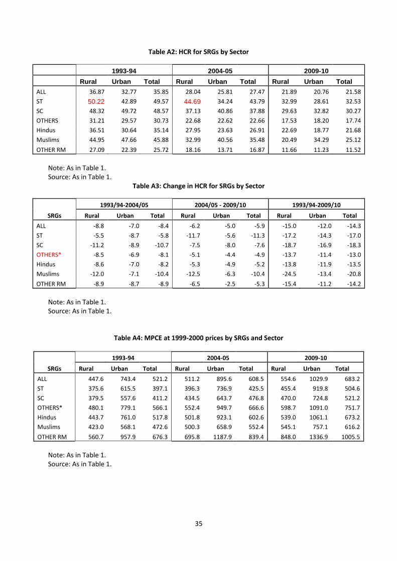
35

Table A2: HCR for SRGs by Sector

1993-94 2004-05 2009-10


ALL 36.87 32.77 35.85 28.04 25.81 27.47 21.89 20.76 21.58

ST 50.22 42.89 49.57 44.69 34.24 43.79 32.99 28.61 32.53

SC 48.32 49.72 48.57 37.13 40.86 37.88 29.63 32.82 30.27

OTHERS 31.21 29.57 30.73 22.68 22.62 22.66 17.53 18.20 17.74

Hindus 36.51 30.64 35.14 27.95 23.63 26.91 22.69 18.77 21.68

Muslims 44.95 47.66 45.88 32.99 40.56 35.48 20.49 34.29 25.12

OTHER RM 27.09 22.39 25.72 18.16 13.71 16.87 11.66 11.23 11.52


Table A3: Change in HCR for SRGs by Sector

SRGs

1993/94-2004/05 2004/05 - 2009/10 1993/94-2009/10


ALL -8.8 -7.0 -8.4 -6.2 -5.0 -5.9 -15.0 -12.0 -14.3

ST -5.5 -8.7 -5.8 -11.7 -5.6 -11.3 -17.2 -14.3 -17.0

SC -11.2 -8.9 -10.7 -7.5 -8.0 -7.6 -18.7 -16.9 -18.3

OTHERS* -8.5 -6.9 -8.1 -5.1 -4.4 -4.9 -13.7 -11.4 -13.0

Hindus -8.6 -7.0 -8.2 -5.3 -4.9 -5.2 -13.8 -11.9 -13.5

Muslims -12.0 -7.1 -10.4 -12.5 -6.3 -10.4 -24.5 -13.4 -20.8

OTHER RM -8.9 -8.7 -8.9 -6.5 -2.5 -5.3 -15.4 -11.2 -14.2


Table A4: MPCE at 1999-2000 prices by SRGs and Sector

SRGs

1993-94

2004-05

2009-10


ALL 447.6 743.4 521.2 511.2 895.6 608.5 554.6 1029.9 683.2

ST 375.6 615.5 397.1 396.3 736.9 425.5 455.4 919.8 504.6

SC 379.5 557.6 411.2 434.5 643.7 476.8 470.0 724.8 521.2

OTHERS* 480.1 779.1 566.1 552.4 949.7 666.6 598.7 1091.0 751.7

Hindus 443.7 761.0 517.8 501.8 923.1 602.6 539.0 1061.1 673.2

Muslims 423.0 568.1 472.6 500.3 658.9 552.4 545.1 757.1 616.2

OTHER RM 560.7 957.9 676.3 695.8 1187.9 839.4 848.0 1336.9 1005.5


36

Table A5: Head Count Ratio By HH Type and SRGs in the Rural Sector

HH Type ST SC OTHERS HINDU MUSLIMS OTHER RM Total

1993-94

SENA 43.6 41.9 30.0 31.7 41.5 18.8 32.9

AGLA 60.2 58.3 49.9 54.0 62.3 48.5 54.4

OLAH 54.5 46.3 37.0 41.7 50.8 31.0 42.2

SEAG 46.0 39.2 26.1 29.7 37.7 16.0 29.7

OTHE 21.0 20.7 17.3 16.5 32.1 12.0 18.1

ALL 50.6 48.6 31.5 36.8 45.2 26.8 37.2

2004-05

SENA 34.3 33.4 20.7 22.6 31.5 7.9 23.8

AGLA 56.0 46.4 39.3 44.0 50.1 36.3 44.1

OLAH 48.0 37.5 27.1 33.5 35.9 17.3 32.7

SEAG 39.9 28.4 17.7 21.5 25.5 13.2 21.4

OTHE 18.4 16.5 13.5 13.1 24.8 6.0 14.3

ALL 44.7 37.1 22.7 28.0 33.0 17.9 28.0

2009-10

SENA 24.2 24.4 15.0 17.7 18.6 6.7 17.4

AGLA 44.7 36.5 31.1 36.5 24.4 22.8 34.7

OLAH 36.5 30.8 20.7 26.9 23.3 6.5 25.5

SEAG 28.2 25.5 13.2 16.5 20.2 12.5 16.6

OTHE 11.1 15.2 6.7 8.9 11.9 1.8 8.8

ALL 33.0 29.6 17.5 22.7 20.5 11.7 21.9


37

Table A6: Change in Poverty Incidence by HH Type and SRGs in the Rural Sector


1993/94 - 2004/05

SENA -9.3 -8.5 -9.3 -9.1 -10.0 -10.9 -9.1

AGLA -4.2 -11.9 -10.6 -10.0 -12.2 -12.2 -10.3

OLAH -6.5 -8.8 -9.9 -8.2 -14.9 -13.7 -9.5

SEAG -6.1 -10.8 -8.4 -8.2 -12.2 -2.8 -8.3

OTHER -2.6 -4.2 -3.8 -3.4 -7.3 -6.0 -3.8

All -5.9 -11.5 -8.8 -8.8 -12.2 -8.9 -9.2

2004/05-2009/10

SENA -10.1 -9.0 -5.7 -4.9 -12.9 -1.2 -6.4

AGLA -11.3 -9.9 -8.2 -7.5 -25.7 -13.5 -9.4

OLAH -11.5 -6.7 -6.4 -6.6 -12.6 -10.8 -7.2

SEAG -11.7 -2.9 -4.5 -5.0 -5.3 -0.7 -4.8

OTHER -7.3 -1.3 -6.8 -4.2 -12.9 -4.2 -5.5

All -11.7 -7.5 -5.2 -5.3 -12.5 -6.2 -6.1

1993/94-2009/10

SENA -19.4 -17.5 -15.0 -14.0 -22.9 -12.1 -15.5

AGLA -15.5 -21.8 -18.8 -17.5 -37.9 -25.7 -19.7

OLAH -18.0 -15.5 -16.3 -14.8 -27.5 -24.5 -16.7

SEAG -17.8 -13.7 -12.9 -13.2 -17.5 -3.5 -13.1

OTHE -9.9 -5.5 -10.6 -7.6 -20.2 -10.2 -9.3

ALL -17.6 -19.0 -14.0 -14.1 -24.7 -15.1 -15.3


38

Table A7: MPCE at Constant (1999-2000) prices By HH Type in the Rural Sector

HH Type/SRG ST SC OTHERS HINDU MUSLIMS ORM Total

1993-94

SENA 421.7 412.9 484.8 471.5 427.2 582.5 468.5

AGLA 324.7 333.3 363.3 344.6 345.0 386.5 346.9

OLAH 367.9 393.2 451.3 425.1 379.1 477.2 422.5

SEAG 390.2 415.9 502.1 472.5 465.8 656.9 480.5

OTHER 553.6 538.1 629.5 615.3 479.2 770.2 609.5

All 374.6 379.7 479.5 443.0 421.0 565.5 446.9

2004-05

SENA 462.7 456.7 582.1 545.1 521.5 849.4 552.4

AGLA 331.7 372.3 398.8 375.7 390.9 436.4 380.0

OLAH 373.6 442.2 507.1 462.3 463.4 600.4 471.5

SEAG 414.6 466.7 564.0 524.4 526.1 774.9 536.1

OTHER 611.6 639.8 779.1 753.7 603.7 945.7 744.5

All 396.2 434.5 552.5 501.9 500.2 697.2 511.3

2009-10

SENA 571.3 501.2 627.3 600.0 530.3 884.4 598.4

AGLA 378.4 403.9 437.9 408.6 476.0 489.1 418.9

OLAH 423.5 455.4 561.3 489.5 511.2 964.6 513.7

SEAG 464.9 507.9 610.1 561.8 567.3 889.3 579.1

OTHE 690.5 657.7 902.2 820.5 748.9 1155.3 835.8

ALL 455.3 469.8 598.7 539.0 545.1 848.2 554.5


39

Table A8: Incidence of Poverty by HH Type and Socioreligious Groups in Urban Sector

HH Type ST SC OTHERS HINDU MUSLIMS ORM All

1993-94

SEMP 51.7 51.7 33.3 32.8 48.6 18.1 35.4

RWSE 31.4 35.8 19.0 20.5 36.9 16.8 21.7

CALA 67.7 71.4 60.8 63.8 68.0 58.4 64.2

OTHER 26.3 38.2 24.6 23.7 39.6 21.4 26.2

Total 43.1 49.5 29.5 30.5 47.9 22.3 32.7

2004-05

SEMP 40.6 45.5 24.4 24.7 39.8 8.8 27.1

RWSE 13.0 25.1 14.6 14.6 34.5 9.1 16.3

CALA 74.5 66.9 52.5 58.1 59.1 52.6 58.0

OTHER 13.5 25.5 13.9 12.6 30.5 6.4 15.0

Total 34.2 40.8 22.6 23.6 40.5 13.5 25.8

2009/10

SEMP 30.0 35.5 20.1 19.2 36.2 7.6 22.1

RWSE 14.8 18.9 9.5 10.1 21.4 7.2 11.1

CALA 61.2 51.9 42.6 45.2 52.6 37.4 46.0

OTHER 21.1 24.6 11.0 12.2 21.9 6.6 13.0

ALL 28.6 32.8 18.2 18.8 34.3 11.2 20.8


Table A9: Change in Incidence of Poverty by HH Type and Socioreligious Groups in Urban Sector


1993/94 - 2004/05

SEMP -11.1 -6.2 -8.8 -8.1 -8.8 -9.3 -8.3

RWSE -18.4 -10.7 -4.4 -5.8 -2.4 -7.7 -5.4

CALA 6.7 -4.5 -8.4 -5.6 -8.9 -5.8 -6.2

OTHER -12.7 -12.7 -10.7 -11.1 -9.1 -15.0 -11.2

ALL -9.0 -8.7 -6.9 -6.9 -7.3 -8.8 -6.9

2004/05-2009/10

SEMP -10.6 -9.9 -4.3 -5.6 -3.7 -1.3 -5.0

RWSE 1.8 -6.2 -5.1 -4.5 -13.1 -1.9 -5.2

CALA -13.3 -15.0 -9.9 -12.9 -6.5 -15.2 -12.0

OTHER 7.5 -0.8 -2.9 -0.4 -8.7 0.2 -2.0

ALL -5.6 -8.0 -4.4 -4.8 -6.3 -2.3 -5.0

1993/94-2009/10

SEMP -21.7 -16.2 -13.2 -13.6 -12.4 -10.6 -13.3

RWSE -16.6 -16.9 -9.5 -10.3 -15.5 -9.6 -10.6

CALA -6.5 -19.5 -18.3 -18.5 -15.4 -21.0 -18.2

OTHER -5.2 -13.5 -13.6 -11.5 -17.8 -14.8 -13.2

ALL -14.5 -16.7 -11.3 -11.7 -13.6 -11.1 -11.9


40

Table A10: MPCE at constant (1999-2000) prices by HH Type and SRGs in the Urban Sector


1993-94

SEMP 565.0 512.0 716.0 716.0 557.0 935.0 694.0

RWSE 700.0 666.0 901.0 867.0 648.0 1085.0 862.0

CALA 417.0 422.0 468.0 456.0 424.0 494.0 452.0

OTHER 727.0 630.0 889.0 891.0 624.0 975.0 853.0

ALL 613.0 559.0 780.0 762.0 565.0 957.0 744.0

2004-05

SEMP 673.0 561.0 875.0 857.0 647.0 1286.0 836.0

RWSE 891.0 789.0 1088.0 1055.0 742.0 1174.0 1031.0

CALA 426.0 452.0 520.0 497.0 476.0 521.0 494.0

OTHER 1001.0 829.0 1288.0 1264.0 856.0 1717.0 1234.0

ALL 737.0 644.0 950.0 924.0 659.0 1190.0 896.0

2009/10

SEMP 838.6 668.4 981.2 979.1 702.2 1344.7 942.2

RWSE 1128.5 882.6 1318.7 1259.4 948.8 1516.3 1243.9

CALA 493.0 512.5 618.2 581.4 579.9 623.3 583.5

OTHER 1056.0 961.4 1399.4 1372.4 949.5 1563.2 1334.8

ALL 919.8 724.8 1091.0 1061.1 757.1 1336.9 1029.9


41

Table A11: MPCE at constant (1999-2000) prices by HH Type and SRGs in the Urban Sector

SRGs Poor Non-poor


1993-94

ALL 255.2 349.1 276.6 560.0 935.8 658.0

ST 245.7 343.2 253.3 506.8 820.1 538.5

SC 250.1 337.2 266.0 500.7 775.1 548.4

OTHERS* 260.1 352.7 285.7 579.9 958.4 690.6

Hindus 253.7 350.6 273.4 553.1 942.5 650.3

Muslims 263.7 342.2 291.6 553.2 773.8 626.1

ORM 263.0 358.9 287.3 671.6 1131.6 811.4

2004-05

ALL 266.4 357.6 288.1 606.6 1082.8 729.9

ST 246.4 326.8 251.7 517.4 950.3 560.9

SC 265.3 350.5 283.9 534.4 846.2 594.4

OTHERS* 273.0 361.7 298.4 634.4 1121.6 774.4

Hindus 264.1 360.8 284.4 594.0 1097.1 719.7

Muslims 279.7 347.6 305.2 609.0 871.4 688.3

ORM 268.5 367.5 292.0 790.6 1318.2 950.4

2009-10

ALL 266.0 353.2 288.7 635.5 1207.2 791.7

ST 249.4 356.0 259.4 556.8 1145.8 622.8

SC 266.5 349.3 284.5 555.7 908.3 623.9

OTHERS* 270.8 354.3 297.4 668.4 1254.9 849.7

Hindus 263.8 355.9 284.3 619.8 1224.0 780.9

Muslims 283.3 344.1 311.1 612.6 972.5 718.5

ORM 269.3 367.1 300.0 924.4 1459.6 1097.4


42

Table A12: Gini Coefficient by Socio-religious Groups and Sector

Socio-religious Groups

1993-94 2004-05 2009-10


ALL 0.30 0.36 0.35 0.30 0.38 0.35 0.31 0.40 0.37

ST 0.28 0.34 0.30 0.27 0.34 0.30 0.28 0.39 0.32

SC 0.26 0.34 0.30 0.26 0.32 0.29 0.26 0.33 0.29

OTHERS 0.30 0.36 0.35 0.30 0.38 0.36 0.32 0.40 0.38

Hindus 0.29 0.36 0.35 0.29 0.37 0.35 0.30 0.40 0.37

Muslims 0.29 0.32 0.32 0.29 0.34 0.31 0.28 0.38 0.33

OTHER RM 0.33 0.39 0.38 0.35 0.37 0.38 0.40 0.41 0.42


Table A13: MPCE of the Poor at Constant (1999-00) prices

(by sector and socioreligious group)

SRGs

1993-94 2004-05 2009-10

Rural Urban Rural Urban Rural Urban

ALL 255.2 349.1 266.4 357.6 266.0 353.2

ST 245.7 343.2 246.4 326.8 249.4 356.0

SC 250.1 337.2 265.3 350.5 266.5 349.3

OTHERS 260.1 352.7 273.0 361.7 270.8 354.3

Hindus 253.7 350.6 264.1 360.8 263.8 355.9

Muslims 263.7 342.2 279.7 347.6 283.3 344.1

ORM 263.0 358.9 268.5 367.5 269.3 367.1


43

Table A14: Distribution of Households across Economic Categories by SRG in 2009/10

HH type/ SRG

Rural

ST SC Others* Hindus Muslims ORM Total

SENA 7.42 14.31 17.14 14.44 24.30 13.54 15.45

AGLA 32.95 37.49 22.21 27.46 23.61 22.99 26.81

OLAH 13.11 20.76 12.99 14.27 18.64 14.42 14.75

SEAG 36.67 17.84 35.52 32.91 21.04 33.35 31.67

OTHE 9.85 9.60 12.13 10.92 12.41 15.70 11.32

ALL 100.00 100.00 100.00 100.00 100.00 100.00 100.00

Urban

ST SC Others* Hindus Muslims ORM Total

SEMP 20.40 29.05 37.67 33.96 48.21 33.67 35.81

RWSE 42.44 37.73 38.86 40.45 28.03 40.51 38.83

CALA 18.91 24.17 11.45 13.46 15.07 11.64 13.55

OTHER 18.25 9.05 12.02 12.14 8.68 14.17 11.81

ALL 100.00 100.00 100.00 100.00 100.00 100.00 100.00

Note: These tables provide distribution of households for each SRG category across economic category, e.g. out of the total ST households in the rural sector in 2009/10, 7.42% were in SENA etc. Source: As in Table 1

44

Appendix 2: Decomposition of Changes in Poverty and Calculation of elasticity It has been pointed out that growth is a necessary condition for reducing poverty. However, it is still being debated as to what is the contribution of growth in reducing poverty? The methodology for finding the contribution revolves around two specific issues. First, there are a large number of studies that attempt to find out the contribution of (economic) growth and change in the distribution of income in the change in poverty incidence. Secondly, several studies try to look into the growth-poverty relationship by calculating the elasticity of reduction of poverty or measuring responsiveness of poverty decline to growth. In this appendix, we briefly describe the methodology used to decompose the changes in poverty in India during 1993/94-2009/10. The elasticity calculation is outlined briefly in section 7. Starting from the pioneering work of Jain and Tendulkar (1990) and Kakwani and Subbarao (1990), decomposition methodology has evolved with insightful contributions by Dutt and Ravallion (1992) and Kakwani (2000). Jain and Tendulkar (1990) and Kakwani and Subbarao (1990) suggested an exact decomposition method in which change in poverty incidence is fully explained by the mean and the redistribution effects. For estimation of poverty incidence for decomposition into the two components, Jain and Tendulkar (1990) used interpolation method to calculate actual and hypothetical poverty measurement while Kakwani and Subbarao (1990) used a polynomial of third degree to represent Lorenz curve within each income class except for the first and last classes for which a Pareto curve is fitted. However, Dutt and Ravallion (1992) argued that the decomposition of change in poverty incidence is unlikely to be exact, suggesting that there will be an unexplained residual. They showed that the residual component can disappear only if the mean or the Lorenz curve remained unchanged over the period. For parametric specifications of Lorenz curve, Dutt and Ravallion (1992) used General Quadratic (GQ) model suggested by Villasenor and Arnold (1989). Kakwani (2000) showed that axiomatically decomposition would always be the exact one. We have used the decomposition methodology as suggested by Dutt and Ravallion (1992) and as refined by Kakwani (2000). First, a parameterized Lorenz curve method is used to derive the actual and hypothetical poverty. For this, Lorenz curve is estimated from the distribution of consumption expenditure. General Quadratic method of estimation of parameters of Lorenz is used as it is more accurate over the entire distribution (Ravallion and Huppi, 1990) and it is also comparatively easier compared to other models, e.g. the Beta model. The Quadratic Lorenz curve is specified as: L(1-L) = a(P2 –L) + b L(P-1) + c(P-L) (1) where L is the cumulative proportion (or percentage) of consumption expenditure, P is the cumulative proportion of population and a, b, c are parameters of Lorenz curve. While estimating parameters of Lorenz curve, the last observation of P and L, which has value (1,1) are excluded since the functional form of Lorenz curve already forces it to pass through point (1,1). Now estimated parameters are used to calculate the actual and hypothetical index of poverty incidence. Poverty incidence is primarily a function of per capita mean consumption expenditure, distribution of consumption expenditure around mean measured by Lorenz curve parameters and exogenously determined poverty line as: P = P (µ, L(p), z) (2)

45

Where µ is the MPCE, L(p) is Lorenz equation and z is exogenously given poverty line. By using estimated parameters, HCR is estimated using the formulae, H=-1/2m [n+ r(b+2z/µ){ (b+2z/µ)2-m}-1/2] (3) Where e= -(a+b+c+1); m = b2-4a; n = 2be-4c; r = (n2-4me2)½ Poverty, P, at two points of time, j and k is given as, Pj = P(µj; πj: z) and Pk = P(µk; πk; z) (4) Where π is the parameters of Lorenz curve and µ and z are the same as above. The change in poverty, ∆P, between the two time periods is ∆Pjk = P (µk; πk; z) - P(µj; πj: z) (5) For decomposition, the actual and the hypothetical poverty index is calculated. Pj and Pk are the actual poverty ratios for periods j and k as both the Lorenz parameters and MPCE is used for the periods j and k, respectively. Next, we calculate hypothetical poverty ratios for the two periods by keeping Lorenz curve constant at jth period and MPCE at the terminal year, i.e. kth period. Next by keeping MPCE constant at jth period level and Lorenz curve at terminal year, kth level. Functional forms for these two cases are: Pjk = P (µk; πj; z) (6) where mean per capita expenditure ‘µ’ is at kth level and Lorenz parameters ‘π’ is used one for base year, and Pjk = P (µj; πk: z) (7) where Lorenz parameters ‘π’ is at kth level and mean per capita expenditure ‘µ’ is at base year level. Kakwani (2000) has shown that the decomposition will be exact as the following in equation holds: ∆Pjk = Ĝjk + Îjk (8) Using eq (9) the mean effect ‘Ĝ’ and eq (10) the distribution effect ‘Î’ is can be calculated as Ĝ = ½[{P (µk, Lj(p), z) – P(µj, Lj(p), z)}+ {P(µk, Lk(p), z) – P(µj, Lk(p), z)}] (9) and Î = ½[{P (µj, Lk(p), z) – P(µj, Lj(p), z)}+ {P(µk, Lk(p), z) – P(µk, Lj(p), z)}] (10)

46

United Nations Development Programme 55 Lodhi Estate, Post Box No. 3059 New Delhi 110003, India Tel: +91 11 46532333 Fax: +91 11 24627612 Email: [email protected] For more information: www.in.undp.org

how inclusive has growth been in india during 1993/94 …€¦ · · 2015-07-312 how inclusive...

Documents