how scale affects eia

How scale affects environmental

impact assessment

Elsa Joao*

Department of Geography, University of Strathclyde, Graham Hills Building, 50 Richmond Street,

Glasgow G1 1XN, Scotland, UK

Received 1 June 2001; received in revised form 1 April 2002; accepted 1 April 2002

Abstract

This paper evaluates the influence of geographical scale on the outcomes of

Environmental Impact Assessments (EIAs). The paper presents results obtained by using

spatial data with different scales for an EIA for a proposed road bypass in Southeast

England (the Hastings Bypass). Scale effects were measured separately for spatial extent

and spatial detail, and were measured both quantitatively using a Geographical

Information System (GIS) and qualitatively using the judgement of EIA experts. The

study found that changes in scale could affect the results of EIAs. For example, the impact

significance and the number of houses affected by air pollution from the road varied

according to the scale used. These observed scale-dependent changes suggest that scale

choice can have important repercussions for the accuracy of an EIA study. This situation is

made more serious when it is recognized that many environmental impact statements (EIS)

fail to mention in explicit terms the scale used. The paper concludes with

recommendations for future practice on how best to control the quality of EIAs in

relation to scale choice.

D 2002 Elsevier Science Inc. All rights reserved.

Keywords: Scale effects; Spatial extent; Amount of detail; Environmental impact assessment; Quality

control

0195-9255/02/$ – see front matter D 2002 Elsevier Science Inc. All rights reserved.

PII: S0195 -9255 (02 )00016 -1

* Tel.: +44-141-548-3601; fax: +44-141-552-7857.

E-mail address: [email protected] (E. Joao).

www.elsevier.com/locate/eiar

Environmental Impact Assessment Review

22 (2002) 289–310

1. Introduction

This paper investigates towhat extent the choice of scale can affect the outcomes

of Environmental Impact Assessments (EIAs). In other words, is it possible that

EIA results are more an artefact of the scale of the data used rather than the situation

in the real world being studied? If that was the case, and the scale effects were

ignored, then there could be serious repercussions for EIA accuracy and quality. To

date, EIA practitioners and researchers have largely ignored this topic. This study

puts scale under the spotlight to stimulate a debate about this important issue.

In this paper the word ‘scale’ is considered to have two key interrelated

meanings relevant to EIAs: scale as spatial extent of the assessment; and scale as

amount of geographical detail or granularity. The two are, however, related, as the

spatial extent of the assessment will usually affect how detailed the assessment will

be, i.e., an EIA of a larger area cannot afford the same amount of detail as a local

assessment. This suggests the existence of a ‘ratio’ between extent and detail that

constrains the data volume that is reasonable to analyse for a particular project

(Goodchild and Quattrochi, 1997). The notion of scale can be applied both to

temporal and spatial aspects, and both are important to EIAs. The research

presented in this paper, however, concentrates on the spatial scale only.

Scale is a key research topic in many disciplines, such as hydrology, archae-

ology and ecology, and much has been written describing the problem of scale and

the methods for studying scaling (e.g., Levin, 1992; Quattrochi and Goodchild,

1997; Tate andAtkinson, 2001; Turner andGardner, 1991;Wiens, 1989). But at the

same time scale remains a complex and misunderstood issue. ‘Scale is one of the

most fundamental yet poorly understood and confusing concepts underlying

research involving geographic information’ (Montello and Golledge, 1999, p. 3).

The importance of scale issues has even led some researchers to propose a new

science of scale (Goodchild and Quattrochi, 1997; Meentemeyer and Box, 1987).

Goodchild and Quattrochi (1997) suggested that a full science of scale would

include: which measures or properties are invariant with respect to scale; methods

to change scale; measures of the impact of scale change; scale as a parameter in

process models; and implementation of multiscale approaches. In this paper, the

emphasis is on measuring the impact of scale change.

Despite its importance, scale has long been a ‘Cinderella topic’ within EIAs.

EIA literature only very rarely addresses the issue of scale and how it can affect the

outcomes of impact assessments.When it does so, it is often couched in the vaguest

of terms. For example, the Canadian Environmental Assessment Agency briefly

commented on the difficulty of identifying spatial boundaries: ‘If large boundaries

are defined, only superficial assessment may be possible and uncertainty will

increase. If the boundaries are small, a more detailed examination may be feasible

but an understanding of the broad context may be sacrificed. Proponents may

perceive assessments with large boundaries as onerous or unfeasible, whereas the

public may think small boundaries do not adequately encompass all of the project’s

environmental effects’ (Canadian Environmental Assessment Agency, 1996, p.

E. Joao / Environmental Impact Assessment Review 22 (2002) 289–310290

13). This paper aims to redress this neglect by focusing exclusively on scale and

EIAs.

Besides a review of academic literature, this study also investigated the

importance of scale issues within EIAs by obtaining information directly from

environmental impact statements (EIS) and from the views of EIA practitioners

themselves. Given the nature of EIAs, where one of the written products is the EIS

itself rather than an academic paper, and where practitioners might not always

express in writing their thoughts on scale issues and EIAs, it was felt that an

exclusive review of academic papers on EIAs would be insufficient. Forty-two UK

EIS were reviewed to find any explicit mentions of scale—none were found. Also,

internet-based discussions with EIA practitioners were established that tapped into

a wide range of EIA expertise from different countries and backgrounds. In total,

during the course of this research, more than 230 research contacts were

established. The review of EIS, and the discussions with practitioners worldwide,

found that EIS, although they cannot escape dealing with scale, often do not state

the scale used explicitly. This is another symptom of the neglect of scale in EIAs. ‘In

my experience, geographical scale is an issue that receives inadequate attention in

the majority of EIS, and in many cases can represent a fundamental limitation to the

production of an effective EIS that provides a defensible basis for the identification

of potentially significant environmental impacts’ (David Broom, SGS United

Kingdom, 1999, personal communication). If scale is not explicitly included,

readers must guess and arbitrarily apply a scale of their own (Allen and Starr, 1982).

As a consequence, and because different scaled models define entities differently,

results using apparently identical models will appear inconsistent.

There is, however, literature on the specific effects of scale on disciplines related

to EIAs, such as water quality (Osterkamp, 1995), landscape studies (Meentemeyer

and Box, 1987), ecology (Fernandes et al., 1999), archaeology (Stein and Linse,

1993), soils studies (Julien and Frenette, 1986), and hydrology (Sposito, 1998). In a

study on land degradation, Gray (1999, p. 330) found that ‘one’s conclusions about

whether land is degraded are influenced by the scope and scale of the analysis. For

example, if we examined changes at the local or regional scale using aerial

photographs, we would most likely arrive at a different conclusion than if we

examined soils at the farm scale. The scale at which studies are undertaken affects

the conclusion because processes and parameters important at one scale may not be

important or predictive at another scale.’

Given the importance of scale in these disciplines it is unlikely in the extreme

that EIAs would be immune from the effects of scale. This is especially relevant,

given that most EIAs are done under strict budgetary and time constraints: ‘In

practice, budgets and schedules often get in the way of using sufficient detail’ (Ron

Bass, Jones and Stokes Associates, USA, 1998, personal communication) and

‘Unfortunately, scale is often directly related to funding. Although the overall

boundary of investigation may be less affected, the detail of investigation will be’

(Tim Huntington, MacAlister Elliott and Partners UK, 1999, personal commun-

ication). If budget and time allows, studies are done with more detail or for larger

E. Joao / Environmental Impact Assessment Review 22 (2002) 289–310 291

spatial extent (ironically, this study has found that this is probably more likely to

happen for small-sized projects with generally fewer impacts). This begs the

question of how many projects are done without sufficient detail and large enough

spatial extent, and how this is affecting the quality of EIAwork.

The potential effect that scale might have on the outcomes of EIAs (e.g., by

influencing the type of impacts found, their magnitude and significance, the type of

mitigation measures recommended, and ultimately the end decision regarding the

proposal) means that it is essential to try to quantify scale effects in EIAs. This

paper describes the results of such a study using an EIA of a controversial road

project. The paper starts by describing the methods used and the results of the

empirical study on the effects of scale on EIAs. The paper concludes with

suggestions on how best to control the quality of scale choice in EIAs.

2. Methods used in the empirical study on the effects of scale on EIAs

For the empirical study, parts of an existing EIA of a road bypass project were

redone using data at different scales to discover how the results differed. Scale

effects were measured separately for extent and detail. In order to measure changes

due to the amount of detail, areas of the same size but different detail were

compared, while to measure scale effects due to changes in spatial extent, areas

with the same detail but different spatial extent were used.

The empirical study consisted of two different but complementary approaches:

one study based on quantitative measurements using a Geographical Information

System (GIS) and a parallel study based on a qualitative analysis by EIA experts.

The inclusion of the qualitative judgements of EIA experts was important because

one of the most common EIA methodologies for evaluating impacts is ‘expert

opinion.’ An exclusively quantitative study of the effects of scale, therefore, would

have only offered a limited view of how scale can affect EIAs.

Through a preliminary investigation of possible UK case studies involving road

projects, seven road EIAs were shortlisted. Of these, the A259 Hastings Eastern

Bypass (6.2 km)was selected (see Fig. 1 for its location in Southeast England). Two

other proposed schemes were related to the Hastings Eastern Bypass: the Bexhill

and Hastings Western Bypass (14.7 km) and the Pevensey to Bexhill Improvement

(4 km) (also seen in Fig. 1). Together these three projects were nearly 25 km long,

which made them one of the longest, and most controversial, road projects in the

UK at the time.1

1 In July 2001, after the research described in this paper was concluded, the proposed Hastings

Bypass was cancelled. This was because of the controversy and strong environmental impacts of the

road project. The UK government reached this decision by using a new ‘multimodal approach’ that

looked at all the alternatives considering all the different modes of transport. This was the first time in

the UK that decisions regarding a road proposal were guided by the new multimodal methodology.


There were three main reasons why a road bypass project was selected for this

research, rather than another type of development such as a new factory. The first

reason had to do with the spatial aspects of road projects. Due to their linear

nature, and potential long length, roads pose interesting challenges related to the

choice of the spatial extent and detail of the study. The second reason was

because roads exert impacts at a range of scales: from localised, direct impacts on

particular areas, through to impacts affecting whole regions due, for example, to

habitat fragmentation and severance of human and wildlife communities. The

final reason had to do with the availability of EIA guidelines. Road projects are

one of the very few types of EIAs for which guidelines exist to advise on the

scale to use. These include the UK Design Manual for Roads and Bridges

(Highways Agency, 1998), and the World Bank publication on roads and the

environment (Tsunokawa and Hoban, 1997).

Data for the Hastings Eastern Bypass case study were obtained by digitising

different source-scale maps and by obtaining data directly from the Ordnance

Survey, the national mapping agency of Great Britain. Table 1 summarizes the

different data sources used for this research. Project EIA is usually done using very

detailed map data, and often culminates with fieldwork. For this reason very

detailed source scales were chosen: 1:10000 and 1:25000. For the 1:10000 scale

map, 1 mm in the map represents 10 m in the terrain, while for the 1:25000 scale

map 1mm in the map represents 25m. The review of EIS carried out (see Section 1)

found that both of these scales are the most common scales used for the EIA of

Fig. 1. Location in Southeast England of the proposed A259 Hastings Eastern Bypass (6.2 km)

(modified from DETR, 1998), and inset showing location of the town of Hastings in the south coast of

the UK.


projects by environmental consultancies in the UK. These two scales are also the

main scales recommended by the UK Highways Agency for the determination of

road impacts (Highways Agency, 1998).

By definition, the two source scale maps portray different amounts of detail or

resolution. The 1:25000 scale map is a generalised version of the 1:10000 scale

map. This means that many geographical features of the 1:25000 scale map would

have been displaced, enlarged, amalgamated or even eliminated (see Joao, 1998).

Other features would have been simplified, i.e., their representation will be

smoother and less sinuous. This means that the same river at the scale 1:25000

might be straighter, and therefore shorter, than at the scale 1:10000. It is worth

pointing out, of course, that even the more detailed 1:10000 is also a generalization

of reality. For example, the Ordnance Survey guidelines for the depiction of water

detail for the 1:10000 scale map state that ‘ponds smaller than 1 mm2 [on the map]

Table 1

Data sources for the empirical study on measuring scale effects on EIA

Data Source and scale

Major environmental features

(e.g., ancient woodland, ponds with

nature conservation value, etc.)

1:25 000 source scale map. Digitised by the author

directly from the mapped information contained in the

Environmental Impact Statement (EIS) of the Hastings

Eastern Bypass (covering one A3 sheet).a

Major environmental features (e.g.,

ancient woodland, ponds with nature

conservation value, etc.)

1:10000 source scale map (complemented by fieldwork

carried out for the EIA). Digitised by the author directly

from the mapped information contained in the EIS of

the Hastings Eastern Bypass (covering four A3 sheets).a

No. of buildings within 200 and 1000 m

of the Hastings Eastern Bypassb1:25000 Ordnance Survey paper map (1997).

No. of buildings within 200, 1000 and

2000 m of the Hastings Eastern Bypass

Land-Line Digital Data from the Ordnance Survey

(Feb 1999)—based on 1:1250, 1:2500 and 1:10000

source scales.c

No. of addresses within 200, 1000 and

2000 m of the Hastings Eastern Bypass

Address-Point Dataset from the Ordnance Survey

(Oct. 1999).d

a Date of publication of the EIS: September 1994.b Buildings had to be counted by hand. Because this was so time consuming, it was not done for

the 2000-m buffer.c Land-Line—is the family name for a range of Ordnance Survey Digital Data products, surveyed

to a high degree of accuracy, that provide detailed information about the topography of Great Britain

such as buildings, kerb-lines, hedges and fences, areas of woodland and even garages and telephone

kiosks (www.ordnancesurvey.co.uk/land-line/) (Ordnance Survey, 1997, 2001).d Address-Point—is a dataset product that uniquely defines and locates residential, business and

public postal addresses in Great Britain. It is created by matching information from Ordnance Survey

digital map databases with more than 25 million addresses recorded in the Royal Mail Postcode

Address File (Ordnance Survey, 2001).


www.ordnancesurvey.co.uk\land-line\

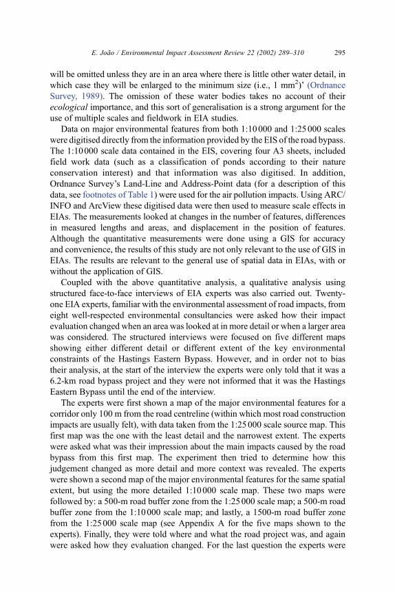
will be omitted unless they are in an area where there is little other water detail, in

which case they will be enlarged to the minimum size (i.e., 1 mm2)’ (Ordnance

Survey, 1989). The omission of these water bodies takes no account of their

ecological importance, and this sort of generalisation is a strong argument for the

use of multiple scales and fieldwork in EIA studies.

Data on major environmental features from both 1:10000 and 1:25000 scales

were digitised directly from the information provided by the EIS of the road bypass.

The 1:10000 scale data contained in the EIS, covering four A3 sheets, included

field work data (such as a classification of ponds according to their nature

conservation interest) and that information was also digitised. In addition,

Ordnance Survey’s Land-Line and Address-Point data (for a description of this

data, see footnotes of Table 1) were used for the air pollution impacts. Using ARC/

INFO and ArcView these digitised data were then used to measure scale effects in

EIAs. The measurements looked at changes in the number of features, differences

in measured lengths and areas, and displacement in the position of features.

Although the quantitative measurements were done using a GIS for accuracy

and convenience, the results of this study are not only relevant to the use of GIS in

EIAs. The results are relevant to the general use of spatial data in EIAs, with or

without the application of GIS.

Coupled with the above quantitative analysis, a qualitative analysis using

structured face-to-face interviews of EIA experts was also carried out. Twenty-

one EIA experts, familiar with the environmental assessment of road impacts, from

eight well-respected environmental consultancies were asked how their impact

evaluation changed when an area was looked at in more detail or when a larger area

was considered. The structured interviews were focused on five different maps

showing either different detail or different extent of the key environmental

constraints of the Hastings Eastern Bypass. However, and in order not to bias

their analysis, at the start of the interview the experts were only told that it was a

6.2-km road bypass project and they were not informed that it was the Hastings

Eastern Bypass until the end of the interview.

The experts were first shown a map of the major environmental features for a

corridor only 100 m from the road centreline (within which most road construction

impacts are usually felt), with data taken from the 1:25000 scale source map. This

first map was the one with the least detail and the narrowest extent. The experts

were asked what was their impression about the main impacts caused by the road

bypass from this first map. The experiment then tried to determine how this

judgement changed as more detail and more context was revealed. The experts

were shown a second map of the major environmental features for the same spatial

extent, but using the more detailed 1:10000 scale map. These two maps were

followed by: a 500-m road buffer zone from the 1:25000 scale map; a 500-m road

buffer zone from the 1:10000 scale map; and lastly, a 1500-m road buffer zone

from the 1:25000 scale map (see Appendix A for the five maps shown to the

experts). Finally, they were told where and what the road project was, and again

were asked how they evaluation changed. For the last question the experts were


asked, overall, what affected their judgement the most—was it the lack of detail or

was it the lack of extent?

3. Results of the empirical study that measured scale effects on EIAs

The changes to the EIAs caused by using maps with different amount of

geographical detail and those caused by maps with varying spatial extent were

measured separately. This section concentrates on the results from that study.

Firstly, the scale effects due to changes in the amount of detail (measured

quantitatively with a GIS) are presented. Secondly, the results of the scale effects

due to changes in spatial extent are shown. The section concludes with the results

from the study where the human experts analysed the five impact maps with

different spatial extent and different spatial detail.

3.1. Scale effects due to changes in the amount of detail

Scale effects due to changes in the amount of detail of the maps fell into three

main categories: (a) changes in the number of features; (b) difference in measured

lengths and areas and; (c) displacement in the position of features. As much as

possible the study concentrated on changes in features that were of environmental

significance, and the ramifications of these changes to the EIAs were made explicit.

3.1.1. Changes in the numbers of features

When all maps are generalised a large number of features can go missing (see

Joao, 1998 for numerous examples). The maps used for the Hastings Eastern

Bypass were no exception. In the cases of the category ‘recent woodland,’ 14 small

individual areas occupying 4.3 ha in the 1:10000 scale map (corresponding to 8%

of the total area occupied by recent woodland), were absent from the 1:25000 scale

map (within 500 m of road centerline). In some case whole feature classes

disappeared. The 1:10000 scale map had nine extra classes (e.g., ponds and

hedges) that were not present in the less detailed 1:25000 scale map. The effects

that the elimination of these features had in the evaluation of impacts are covered in

the human experts’ Section 3.3.

In the original Hastings EIS report, the most quantitative analysis was carried

out on potential air pollution. Because this was the environmental impact that relied

most on direct map measurements it was chosen as the key quantitative variable on

which to study the elimination of features. According to the UKHighways Agency

(1998, Section 3, part 1, page 6/1), in order to assess air quality ‘mark on a map of a

scale in the range 1:25000 to 1:10000 all buildings or areas where people might

possibly be subjected to a change in air quality. Only properties or areas within 200

m of the route or corridor need to be considered.’ This method advocated by the

Highways Agency, and used by most UK environmental consultancies when

conducting an EIA of road projects, requires that the number of properties be used


as a surrogate for population. It is assumed by the UK Highways Agency that

beyond 200 m the contribution of vehicle emissions is not significant because air

pollutants return to background levels.

The process used for the assessment of air-quality impacts was therefore a

powerful way of studying how specific changes in the number of features could

affect an EIA. Table 2 shows the results of calculating the number of buildings for

the two map scales recommended by the Highways Agency (1998) method.

Because more buildings are found when using the Land-Line data, air-pollution

impacts look more serious when using this data source than when using the

1:25000 scale map. So, depending on which one of these two scales is used,

different alternative routes might be selected in order to reduce air pollution

impacts caused by the road.

In addition to the 1:10000 and 1:25000 scale data, the table also shows the

results when using postcode addresses. This last data source was used because it is

considered bymany researchers to be amore accurate way of estimating population

than using maps (Raper et al., 1992). Surprisingly, the number of address point

seeds was less than the number of buildings in the very detailed Land-Line data.

Because there are multiple addresses in high-rise buildings, the opposite was

expected, i.e., that there would be more addresses than there were buildings. This

unexpected result was due to the way ‘building seeds’ are classified in the Land-

Line digital data. It covers all buildings with a minimum dimension of 5 m but this

includes uninhabited buildings such as greenhouses, detachedmonuments, cooling

towers and water tanks! Counterintuitively, in this example, the less detailed

1:25000 scale map (where less important buildings have been eliminated or

amalgamated) was therefore more accurate than the 1:10000 scale data for

calculating the population exposed to air pollution from the new road. This result

is useful in highlighting the importance of data quality for analysis, especially when

fieldwork is not available to corroborate the true meaning of map features.

3.1.2. Difference in measured lengths and areas

The quantitative analysis of key environmental linear and areal features also

demonstrated extensive changes for maps of different geographical detail. In order

to compare changes in lengths and areas, only features that were common to both

scales were used. For linear features, the length of the boundary of the Area of

Table 2

Number of buildings for different scales when measuring air pollution within 200 m of the Hastings

Eastern Bypass (6.2 km long)

1:25000

paper map

OS Land-Line digital

data (based on 1:1250,

1:2500 and 1:10000 scales)

Address-point

seeds

No. of buildings within 200 m

of the Hastings Eastern Bypass

56 160 58


Outstanding Natural Beauty (AONB) was 14% shorter in the less detailed map as

the line was simplified and therefore made less sinuous. However, the very straight

Roman road increased in length by 23% on the 1:25000 scale map, due mainly to

the EIS extending the length of the line to the wrong point.

For areal features there was very large variation in the changes in size (see Fig.

2). Of the 37 individual features common to both maps, 24 increased in area and 13

decreased in area. In general, areas got larger as the outline of areas got less

convoluted (see Fig. 3, which shows how an area of ancient woodland increased

from 22.9 to 26 ha) or small areas were exaggerated. The most dramatic increase in

areas (for example, feature 20 in Fig. 2, a recent woodland, nearly tripled in size)

were all due to very small features being enlarged in the less detailed map so that

they would not be eliminated. This is a common effect of map generalisation—see

the Ordnance Survey example on the guidelines for the depiction of water detail in

Section 2. The four areal features that increased the most (features 10, 17, 20 and 26

Fig. 2. Percentage change of area and perimeter for the 37 individual areas common to both 1:10000

and 1:25000 scales, for the zone 500 m from the proposed road centreline. The graph shows the

change in the features in the 1:25000-scale map in relation to the 1:10000 scale.


in Fig. 2) were the four smallest features. The cases where areas got smaller were

usually due to small or narrow peninsula-type shapes and small sections disappear-

ing on the less detailed scale.

One of the key impacts of the Hastings bypass was on the important ancient

woodland present along the route of the proposed road. Depending on the scale

used, the area of the woodland affected would vary. For example, the area of

ancient woodland within 500 m of the road using the 1:25000 scale map was 91.2

ha, while for the 1:10000 scale map the area was 87.5 ha. This means that the

impacts of the destruction and potential disturbance of ancient woodland for the

proposed Hastings road bypass could be found to be slightly more serious when

measured using the less detailed 1:25000 scale map. While the absolute difference

is small, if there was a threshold involved then the difference in areas could play a

crucial role.

3.1.3. Displacement of features

Displacement of features means that the features are not in the same geograph-

ical position in the two maps and this introduces errors of positional accuracy and

affects any subsequent spatial analysis. For example, it may affect which features

fall in or out of an impact zone and it can strongly alter the results of a map overlay

to determine, for example, the areas that will suffer the most cumulative impacts

(see Joao, 1998). In this study, there were several instances when displacement in

the position of features was observed between the two scales. The 14 listed

buildings (common to all maps) suffered, on average, 23.4 m displacement

(ranging from 9.4 to 42.8 m), while the Roman road had a maximum displacement

of 90.5 m and the boundary of the AONB had a maximum displacement of 51.1 m

(for a definition of maximum vector displacement see McMaster, 1987).

Displacement can lead to either finding false relationships between the data

or lead to a failure in finding important relationships that matter. In one case,

because of the close proximity between the Roman road and five listed

buildings, an environmental consultant interviewed judged that there could be

a possible archaeological relationship between the Roman road and the

Fig. 3. An area of ancient woodland measured using different source scale maps (although displayed

here at the same scale)—the feature labelled 1 in Fig. 2.


buildings, indicating an important archaeological area. However, that relation-

ship was no longer evident at the 1:10000 scale due to the different relative

positions of the features (see Fig. 4). This meant that at the scale 1:25000 the

area was considered more important archaeologically and, as a consequence,

the impacts of the road bypass would be found to be more serious than if the

study had been done at the 1:10000 scale.

3.2. Scale effects due to changes in spatial extent

In order to measure scale effects due to changes in spatial extent, areas

with the same detail but different spatial extent were compared. The main

effect on EIAs is how it influences the determination of the level of impact

significance, i.e., how important the impact is deemed to be. If only a small

spatial extent is considered, and a particular resource is widely available

within that small extent, then it would be assumed that losing part of that

locally abundant resource is not very important. If, however, a wider area is

studied and it is found that this resource is rare at a regional or national

level, then the same amount of resource loss would have a relatively greater

importance and the impact significance is deemed to be high.

This can be expressed quantitatively using the example in Table 3. In this

case, as the extent increases and more urban areas are included, the

percentage of population affected by air pollution decreases, and the impacts

therefore appear to take on less importance (when the study area is 1000 m

Fig. 4. Change in the position of five listed buildings (the black squares) and the Roman road (the

dashed line) for two different source scale maps (although displayed here at the same scale).


from the road centreline 3.5% of the population is affected by air pollution,

but when the study area is increased to 2000 m from the road centreline only

0.8% of the study population is affected by air pollution). The opposite could

also happen—the impacts could look more serious if fewer urban areas were

included when the area looked at was increased. Therefore, the homogeneity

of the study area has a role to play—if the area was completely homogen-

eous, then no such difference would occur.

This relationship means that it is possible to manipulate the results according

to the size of the area studied. Ross (1998, p. 271) noted this in relation to

cumulative effects assessment (CEA):

The greater the area assessed for CEA, the smaller will be the percentage of

impacts caused by the project, because more other sources of impact get

captured in the analysis. While I would not suggest this happens on purpose (a

proponent wishing to have it appear that a project causes only a small portion

of the impact), it is an interesting feature of this and other regionally based

CEAs.

The possibility of cynical manipulation of results according to the detail used or

the size of the area studied is obviously of crucial importance. A solution to this

problemmight be to set up guidelines or rules that give advice on suitable scales for

analysis (see Section 4). The Inter-American Development Bank, for example,

started to demand the use of particular scales in the ‘terms of reference’ both for

analysis and for presentation of the results, and as a consequence noted an

improvement in the quality of the EIA work (Luis Miglino, Inter-American

Development Bank, USA, 1998, personal communication). This was prompted

by the case of corrupt enterprises in Brazil that were using maps of poor detail to

help them get work commissioned—bearing in mind that the criteria of selection is

often to minimise cost and producing, say, a geologic map at the 1:50000 scale is

more expensive that at 1:500000 scale.

3.3. Study on the effects of scale on EIAs using human experts

Coupled with the above quantitative measurements, EIA experts were

asked to evaluate road impacts by analysing five different maps (see

Table 3

Percentage of addresses, of different-sized study areas, affected by air pollution caused by the Hastings

Eastern Bypass

No. of address-point seeds % affected by air pollution

Area within 200 m of road centreline 58 100

Area within 1000 m of road centreline 1653 3.5

Area within 2000 m of road centreline 7101 0.8

Note: It is assumed that only addresses within 200 m of the road centreline are affected by air pollution.


Appendix A) to see how their evaluation changed for different size areas and

areas with different detail. As more detail and greater spatial extent were

provided, a wider range of features and issues appeared. Most experts felt that

the impacts looked more serious both with increased detail and with increased

extent. The new features that appear with each new map can be seen in Table

4. With the exception of the 500-m buffer zone using the 1:10000 source

Table 4

Features that appeared when more detail or more extent was given to the EIA experts

Sequence of maps

given to experts

Initial features New features that had not

appeared before on any of the maps

Map 1: 100-m buffer zone, 1. Ancient woodland

1:25000 source scale map 2. Recent woodland

3. Copses and shaws—

possible ancient woodland

4. Conjectured Roman road

Map 2: 100-m buffer zone,

1:10000 source scale map

1. Grassland of nature conservation

interest

2. Pond of nature conservation

interest

3. Archaeological find-scatter,

identified from field walking

4. Line of trees

5. Hedges

6. Public footpath

7. Archaeological earthworks

8. Archaeological site

9. Archaeological find-spot

Map 3: 500-m buffer zone, 1. Public open space/recreation area

1:25000 source scale map 2. Archaeological significant area

3. Southern boundary of the Area of

Outstanding Natural Beauty (AONB)a

4. Listed building

5. Sites from ‘Sites and Monuments

Record’





1. Sites of Special Scientific

Interest (SSSI)b

2. Scheduled ancient monument

a The primary purpose of the AONB designation is to conserve natural beauty. Since 1949, 14%

of the countryside of England and Wales has been given AONB status. AONB are of national as well

as local importance.b SSSI are the finest sites for wildlife and natural features in England (covering approximately 8%

of England), supporting many characteristic, rare and endangered species, habitats and natural

features. SSSI are areas of national or international importance.


scale map, all maps presented the expert with some new information.

Particularly noteworthy, as observed by most experts were: the hedges,

footpaths and features of conservation interest that only appear on the

1:10000 scale map; the southern boundary of the AONB that only appears

with the 500-m buffer; and the two Sites of Special Scientific Interest (SSSI)

that only appear with the 1500-m buffer zone.

Overall the experts felt that it was the lack of spatial extent, rather than

lack of detail, that affected their judgement more. ‘In terms of EIA, context is

everything’ (Ruth Kelly, Environmental Resources Management, UK, 1999,

personal communication). As the consultants explained, they are accustomed

to evaluating sites with very limited data: ‘you can sort the detail in your

mind very quickly but what you can’t do is form any view of where it is and

what is the context you’re dealing with’ (Jon Grantham, Land Use Con-

sultants, UK, 2000, personal communication). It was even suggested by one

of the experts that information provided by using wider spatial extent could

be used to complement detail. For example, the existence of archaeological

sites within a wider extent (as wide as a 1-km buffer zone) can be used to

conjecture whether there might be archaeologically significant areas within the

narrow corridor of 100 m. This finding indicates that it is necessary to assess

environmental impacts with sufficient extent, otherwise the real importance of

a site might be disguised. Widening the study area supports the recommenda-

tion by English Nature to have all proposed roads evaluated with a minimum

buffer of 500 m and a maximum of 2000 m, on each side of the road (Bina

et al., 1995). An area this size is considerably larger than the recommendation

by the UK Highways Agency of using a 100-m buffer zone as the maximum

distance needed to calculate disruption due to construction.

Presented with the 100-m buffer most experts felt very uncomfortable and

stated that they could not do a fair judgement with such a narrow extent.

Some expressed how it was problematic to evaluate the significance of the

impacts. For example, it was not possible to determine the percentage of

woodland areas affected. It was also impossible to know if the road was

passing through the middle of an area of ancient woodland or if it was

merely cutting an edge of the woodland. It was also difficult to evaluate

alternatives with such a narrow corridor. ‘Can’t do any evaluation with just

100 m buffer—woodlands might only be 100 m wide—if so then you could

go around them’ (Philip Cumming, Dames and Moore, UK, 2000, personal

communication).

Although less so than in relation to lack of extent, some experts also felt

uncomfortable with the lack of the detail. With more detail, the majority of

experts felt that the impacts looked more problematic than before. ‘A key issue in

EIA is that the more you look, the more you find. This means that a site that is

looked at in more detail might appear more precious than other sites’ (Jon

Grantham, Land Use Consultants, UK, 2000, personal communication). With

increasing detail, it looked as if the road would have potential impacts along its


whole route while previously only the west area seemed problematic. ‘My first

impressions were wrong. I originally assumed that only the first two kilometres of

the road were vulnerable to impacts. With the extra detail it became obvious that

the whole length of road was an issue’ (Ana Teresa Chinita, PROCESL, Portugal,

1999, personal communication).

The experts’ analysis on the seriousness of impacts caused by the proposed

new road was affected by both different spatial extent and different geographical

detail. This finding, coupled with the quantitative measurement of scale effects in

EIAs, strongly supports the need for improved practice regarding how scale

issues are currently taken into account in EIAs.

4. Conclusions and recommendations for future practice

To the author’s knowledge, this was the first time an empirical study had been

carried out specifically to determine whether scale could affect the accuracy of

impact prediction. Parts of an existing EIA of a road project (the Hastings Eastern

Bypass in Southeast England) were redone at different scales to discover how the

results differed. Two complementary approaches were used: one study based on

measurements using a GIS, and a parallel study based on analysis by EIA experts.

Both aspects of the study found that changes in scale, in terms of detail and spatial

extent, can have important repercussions on the results of EIAs, such as in the

determination of impact significance and the measurement of environmental

parameters.

The ultimate consequence of the changes in EIA results, according to scale, is

that the outcomes of EIAs can be altered. A different EIA outcome might be, for

example, how much longer the road would need to be to avoid sensitive or

protected features apparent at one scale and not another. This means that,

according to the scale used, different decisions might be taken regarding the

proposal, or different alternatives might be chosen, or different mitigation

measures might be implemented. This is the ultimate ‘impact’ of scale in EIA.

It is impossible to know for sure whether the EIA of the Hastings Bypass would

have come to a widely differing conclusion overall if different scales had been

used. However, this study has demonstrated important scale effects such as in the

area of woodland affected, the importance of archaeological sites, and the number

of buildings affected by air pollution. The impact that these scale effects would

then have on the final outcome of the EIA would depend on the methodology

used for deciding on alternatives or what mitigation measures should be applied.

A quantitative methodology based on thresholds would be more sensitive even to

small changes in the determined values of impact significance or the measured

environmental parameters.

It may be argued that for most project EIAs, fieldwork would complement

and correct any incomplete or wrong information given in mapped data. If

this were always the case, scale effects might not manifest themselves as


seriously. For example, the number of houses within 200 m of a road might

be counted one by one in the field. This, however, would only apply to scale

effects caused by changes in detail and would not apply to the scale effects

caused by changes in spatial extent. It can also be argued that scale effects

(for both detail and spatial extent) will always be relevant in that (a) the field

study might not cover all areas; (b) scale influences the desk study, which in

turn affects the design of fieldwork; (c) the fieldwork itself is carried out

using a map (either paper copy or a digital copy on the computer screen) as a

base, with information added directly to the map in the field (such as in the

case of the 1:10000 source data used in this study); and (d) spatial scale will

always affect assessments that rely strongly on mapped information, such as

very large projects, cumulative effects assessment, and strategic environmental

assessment. Above all, it is crucial that practitioners are aware of the dangers

of ignoring scale effects in EIA or of being uncritical in relation to the choice

of scale. ‘Spatial scale is a last consideration in many studies, yet scale often

selects the nature of the results’ (Meentemeyer and Box, 1987, p. 22).

This research has discovered that scale, in terms of both detail and extent,

is an important issue that, to date, has been largely neglected in EIA. For this

reason, it is necessary to devise ways of improving existing environmental

assessments by taking scale into account. A key recommendation for future

practice is that the choice of scale in EIA should be public and transparent.

‘Scale is not a property of nature alone but, rather, is something associated

with observation and analysis’ (Allen and Hoekstra, 1991, p. 48). This means

that the chosen scale is one part of the observer bias, and therefore it is

fundamental to define the scale of observation. In other words, scale choice

should be explained, justified and explicitly stated in all EIS. Otherwise one

cannot accurately compare different environmental impact assessments or even

choose between them when they differ.

Another recommendation is that it is necessary to investigate the need for

new EIA guidelines on scale. These guidelines could be of three different

types: general qualitative recommendations (e.g., ‘Terms of reference should

consider scale issues explicitly’); specific quantitative guidelines linked to

processes (when possible) (e.g., ‘In reporting landscape pattern, grain should

be two to five times smaller than the spatial features of interest,’ O’Neill et

al., 1996, p. 169); and, ‘scale warnings’ indicating scales to be avoided (e.g.,

‘Map scales of less detail than 1:250000 should be avoided for baseline

studies of project EIA’). Where it is not possible or sensible to impose strict

rules like ‘100 m either side of a road,’ the scale guidelines could be

procedural rather than prescriptive.

A key aspect of these guidelines is the realisation that there isn’t necessarily

one ‘right’ scale but that there are instead multiple or a range of scales appropriate

for the description of a system. Although it might be unclear as to the ‘right’ set

of scales to use, it may be known which scales should be avoided. ‘That there is

no single correct scale or level at which to describe a system does not mean that


all scales serve equally well or that there are not scaling laws’ (Levin, 1992, p.

1960). What is fundamental is to recognise that, because change is taking place

on many scales, multiscale approaches might be required, and that we need ‘to

understand the consequences of suppressing or incorporating detail’ (Levin,

1992, p. 1947).

Future research will investigate multiscale approaches in EIAs and will propose

new scale guidelines in EIAs for both spatial and temporal aspects. Another major

line of research is the need to compare scale issues for project EIAs with strategic

environmental assessment (SEA). If SEA is defined prior to the EIAs of individual

projects, ensuring the SEA is as accurate as possible can be argued to be at least as

important (if not more).

Acknowledgments

This research was financed by a fellowship of the ESRC Global Environ-

mental Change Programme (Award Number L32027307397). I also would like to

thank the comments from three anonymous referees and the many EIA

practitioners and scale researchers around the world for their ideas, suggestions

and advice.

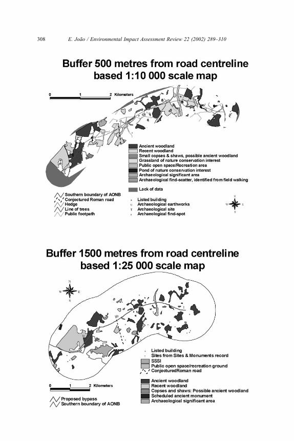
Appendix A. The five maps shown in sequence to the EIA experts

Note: Colour versions of these maps can be found in http://www.geog.gla.

ac.uk/~ejoao/maps.pdf


http:\\www.geog.gla.ac.uk\~ejoao\maps.pdf

References

Allen T, Hoekstra T. Role of heterogeneity in scaling of ecological systems under analysis. In: Kolasa

J, Pickett S, editors. Ecological heterogeneity. New York: Springer-Verlag; 1991. p. 47–68.

Allen TFH, Starr TB. Hierarchy: perspectives for ecological complexity. London: University of

Chicago Press; 1982.

Bina O, Briggs B, Bunting G. The impact of Trans-European Networks on nature conservation: a pilot

project. Bedfordshire: The Royal Society for the Protection of Birds; January 1995.

Canadian Environmental Assessment Agency. A reference guide for the Canadian Environmental

Assessment Act: assessing environmental effects on physical and cultural heritage resources. Hull,

Quebec: Canadian Environmental Assessment Agency; 1996.

DETR. A new deal for transport better for everyone—the government’s white paper on the future of

transport. London: Department of Environment, Transport and the Regions; 1998.

Fernandes TF, Huxham M, Piper SR. Predator caging experiments: a test of the importance of scale. J

Exp Mar Biol Ecol 1999;241:137–54.

Goodchild MF, Quattrochi DA. Introduction: scale, multiscaling, remote sensing, and GIS. In: Quat-

trochi DA, Goodchild MF, editors. Scale in remote sensing and GIS. Boca Raton, FL: Lewis

Publishers; 1997. p. 1–11.

Gray LC. Is land being degraded? A multi-scale investigation of landscape change in Southwestern

Burkina Faso. Land Degrad Dev 1999;10:329–43.

Highways Agency. Manual of highways, roads and bridges—environmental assessment, vol. 11.

London: HMSO; 1998 (First published in 1993, updates for 1994 and 1998).

Joao E. Causes and consequences of map generalisation. London: Taylor & Francis; 1998.

Julien P, Frenette M. Scale effects in predicting soil erosion. In: Hadley R, editor. Drainage basin

sediment delivery. IAHS-AISH Publ., vol. 159. 1986. p. 253–9 (Proceedings Symposium, Albu-

querque).

Levin S. The problem of pattern and scale in ecology. Ecology 1992;73(6):1943–67.

McMaster R. The geometric properties of numerical generalisation. Geogr Anal 1987;19(4):330–46.

Meentemeyer V, Box E. Scale effects in landscape studies. In: Turner MG, editor. Landscape hetero-

geneity and disturbance. New York: Springer Verlag; 1987. p. 15–34.

Montello DR, Golledge R. Scale and detail in the Cognition of Geographic Information—report of a

specialist meeting held under the auspices of the Varenius Project. Santa Barbara, CA: National

Centre for Geographical Information and Analysis; 1999.

O’Neill R, Hunsaker C, Timmins S, Jackson B, Jones K, Riitters K, Wickham J. Scale problems in

reporting landscape pattern at the regional scale. Landsc Ecol 1996;11(3):169–80.

Ordnance Survey. Ordnance survey specification module 7E for the 1:10000 scale map. Internal

Guidelines, most recent amendment June 1989. Southampton: Ordnance Survey; 1989.

Ordnance Survey. Land-Line user guide reference section. Southampton: Ordnance Survey; 1997.

Ordnance Survey. Business catalogue 2001. Southampton: Ordnance Survey; 2001.

Osterkamp W, editor. Effects of scale on interpretation and management of sediment and water

quality. IAHS Publication vol. 226. Wallingford, UK: International Association of Hydrological

Sciences, 1995.

Quattrochi DA, Goodchild MF, editors. Scale in remote sensing and GIS. Boca Raton, FL: Lewis

Publishers; 1997.

Raper J, Rhind D, Shepherd J. Postcodes: the new geography. Harlow: Longman Scientific and

Technical; 1992.

Ross W. Cumulative effects assessment: learning from Canadian case studies. Impact Assess Proj

Apprais 1998;16(4):267–76.

Sposito G, editor. Scale dependence and scale invariance in hydrology. Cambridge, New York: Cam-

bridge University Press; 1998.

Stein JK, Linse AR, editors. Effects of scale on archaeological and geoscientific perspectives. Boulder,

CO: Geological Society of America; 1993.


Tate N, Atkinson M, editors. Modelling scale in geographical information science. Chichester: Wiley;

2001.

Tsunokawa K, Hoban C, editors. Roads and the environment: a handbook. Washington, DC: World

Bank; 1997.

Turner MG, Gardner RH, editors. Quantitative methods in landscape ecology: the analysis and

interpretation of landscape heterogeneity. New York: Springer Verlag; 1991.

Wiens J. Spatial scaling in ecology. Funct Ecol 1989;3:385–97.


how scale affects eia

Documents