how the cbo works jonathan lewis

How the CBO works

Jonathan Lewis

www.jlcomp.demon.co.uk

© Jonathan Lewis2001 - 2003

NoCOUG 2003

Who am I

Independent Consultant.

18+ years experience.

Design, Strategy, Reviews, Briefings, Seminars, Tutorials, Trouble-shooting

www.jlcomp.demon.co.uk


NoCOUG 2003

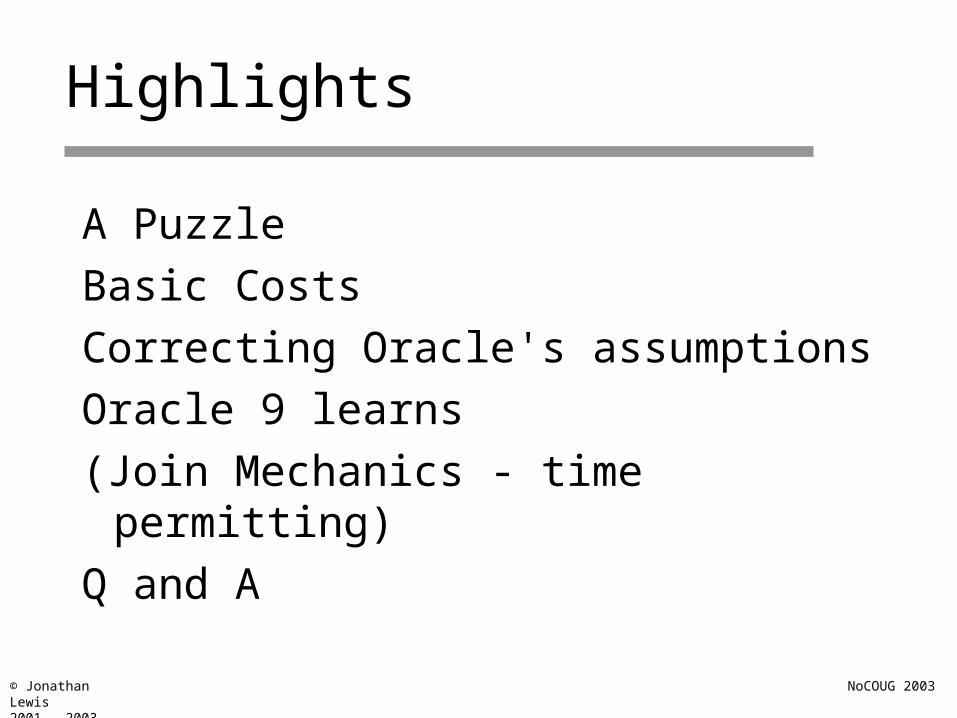
Highlights

A Puzzle

Basic Costs

Correcting Oracle's assumptions

Oracle 9 learns

(Join Mechanics - time permitting)

Q and A


NoCOUG 2003

A puzzle (v8.1 - 4K)

create table t1 asselect

trunc((rownum-1)/15) n1, trunc((rownum-1)/15) n2, rpad('x',100) v1

from all_objects where rownum <= 3000;

create table t2 asselect

mod(rownum,200) n1, mod(rownum,200) n2, rpad('x',100) v1

from all_objects where rownum <= 3000;

We construct two sets of data with identical content, although we do use two different mathematical methods to get 15 rows each for 200 different values.


NoCOUG 2003

A puzzle - indexed

create index t_i1 on t1(n1);

create index t_i2 on t2(n1);

analyze table t1 compute statistics;

analyze table t2 compute statistics;

We create indexes and generate statistics. In newer versions, we should use the dbms_stats package, not analyze. (Note- compute is often over-kill)


NoCOUG 2003

A puzzle - checking data

USER_TABLESTABLE_NAME BLOCKS NUM_ROWS AVG_ROW_LEN----------- ------ ---------- -----------T1 96 3000 111T2 96 3000 111

USER_TAB_COLUMNSTAB COL LOW_VALUE HIGH_VALUE NUM_DISTINCT--- ---- --------- ---------- ------------T1 N1 80 C20264 200T2 N1 80 C20264 200

We can check that statistics like number of rows, column values and column counts are identical. The data contents is identical across the two tables.


NoCOUG 2003

A puzzle - the problem

select * from t2 where n1 = 45;

SELECT STATEMENT Optimizer=CHOOSE (Cost=15 Card=15) TABLE ACCESS (FULL) OF 'T2' (Cost=15 Card=15)


SELECT STATEMENT Optimizer=CHOOSE (Cost=2 Card=15) TABLE ACCESS (BY INDEX ROWID) OF 'T1' (Cost=2 Card=15) INDEX (RANGE SCAN) OF 'T_I1' (NON-UNIQUE) (Cost=1 Card=15)

We now run exactly the same query against the two sets of data - with autotrace switched on - and find that the execution plans are different.


NoCOUG 2003

A puzzle - force it

select /*+ index(t2) */ * from t2 where n1 = 45;




Why has Oracle ignored the index on T2 ? Put in the hint(s) to make it happen, and see if we get any clues. The cost of a tablescan is cheaper !


NoCOUG 2003

A puzzle - the detail

select table_name tab,num_rows num_rows, avg_leaf_blocks_per_key l_blocks, avg_data_blocks_per_key d_blocks, clustering_factor cl_fac

from user_indexes;

TAB NUM_ROWS L_BLOCKS D_BLOCKS CL_FAC---- -------- -------- -------- ------T1 3000 1 1 96T2 3000 1 15 3000

Why is the tablescan cheaper ? We look at the data scattering, rather than the data content, and find the answer. The clustering is different.


NoCOUG 2003

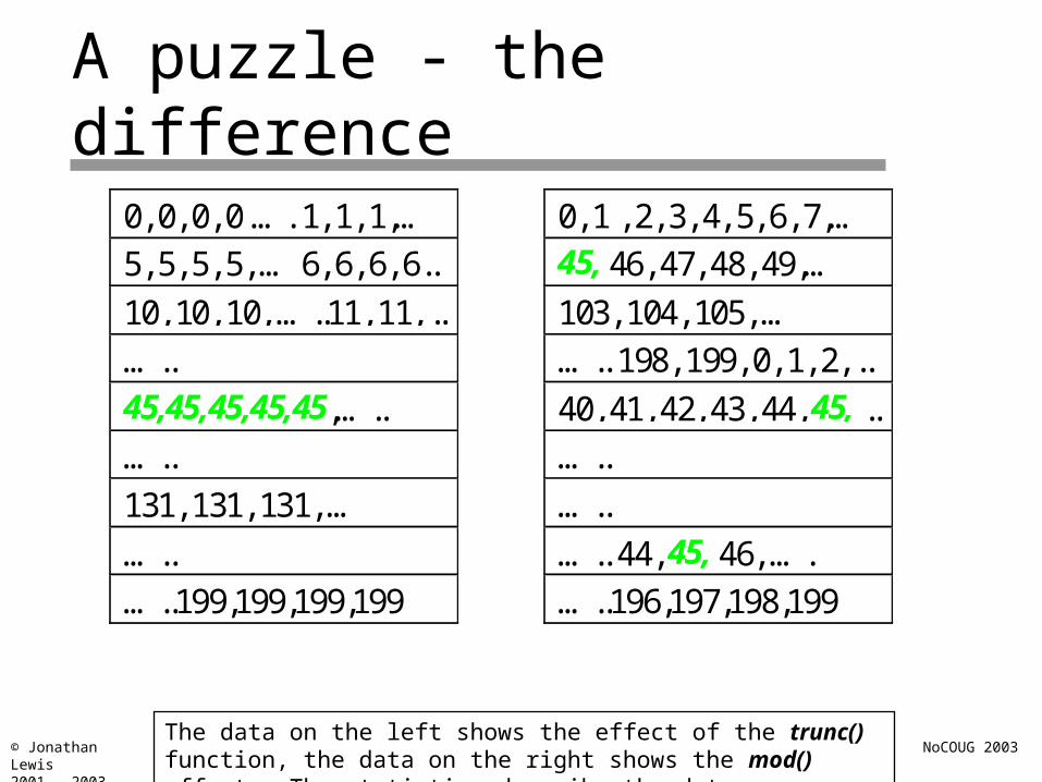
A puzzle - the difference

0, 0, 0, 0 …. 1, 1, 1,…

5, 5, 5, 5, … 6, 6, 6, 6..

10, 10, 10, …..11, 11, ..

…..45,45,45,45,45,…..46,46,..…..

131, 131, 131, …

…..

…..199,199,199,199

0, 1 , 2, 3, 4, 5, 6, 7,…45, 46, 47, 48, 49,…

103, 104, 105, …

….. 198, 199, 0, 1, 2, ..

40, 41, 42, 43, 44, 45, ..

…..

…..

….. 44, 45, 46, ….

…..196,197,198,199

The data on the left shows the effect of the trunc() function, the data on the right shows the mod() effect. The statistics describe the data perfectly.


NoCOUG 2003

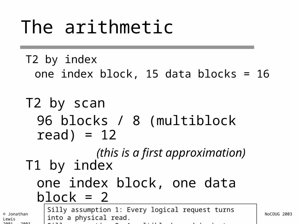
The arithmetic

T2 by indexone index block, 15 data blocks = 16

T2 by scan96 blocks / 8 (multiblock read) = 12

(this is a first approximation)

T1 by indexone index block, one data block = 2

Silly assumption 1: Every logical request turns into a physical read. Silly assumption 2: A multiblock read is just as fast as a single block read.


NoCOUG 2003

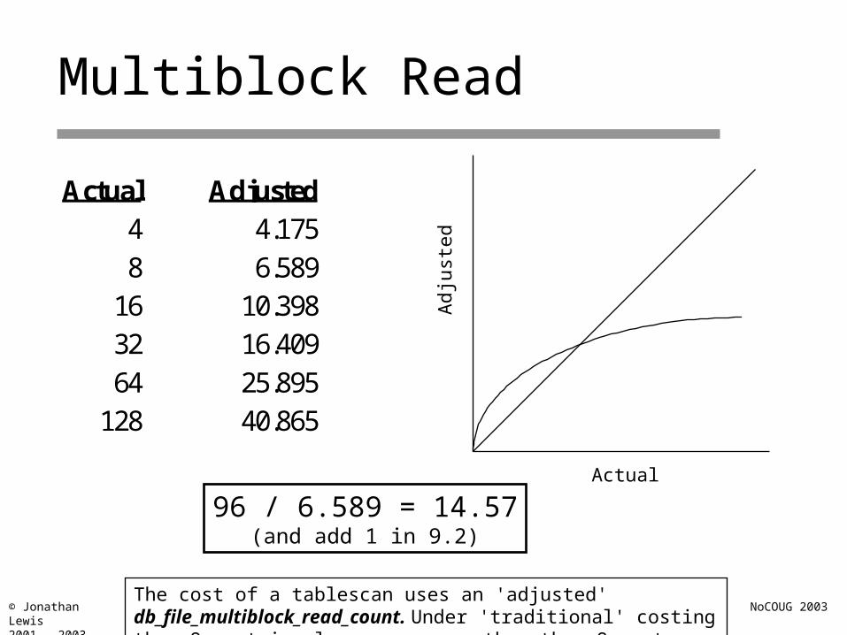
Multiblock Read

Actual Adjusted4 4.1758 6.589

16 10.39832 16.40964 25.895

128 40.865

Actual

Adj

uste

d

96 / 6.589 = 14.57(and add 1 in 9.2)

The cost of a tablescan uses an 'adjusted' db_file_multiblock_read_count. Under 'traditional' costing the v9 cost is always one more than the v8 cost..


NoCOUG 2003

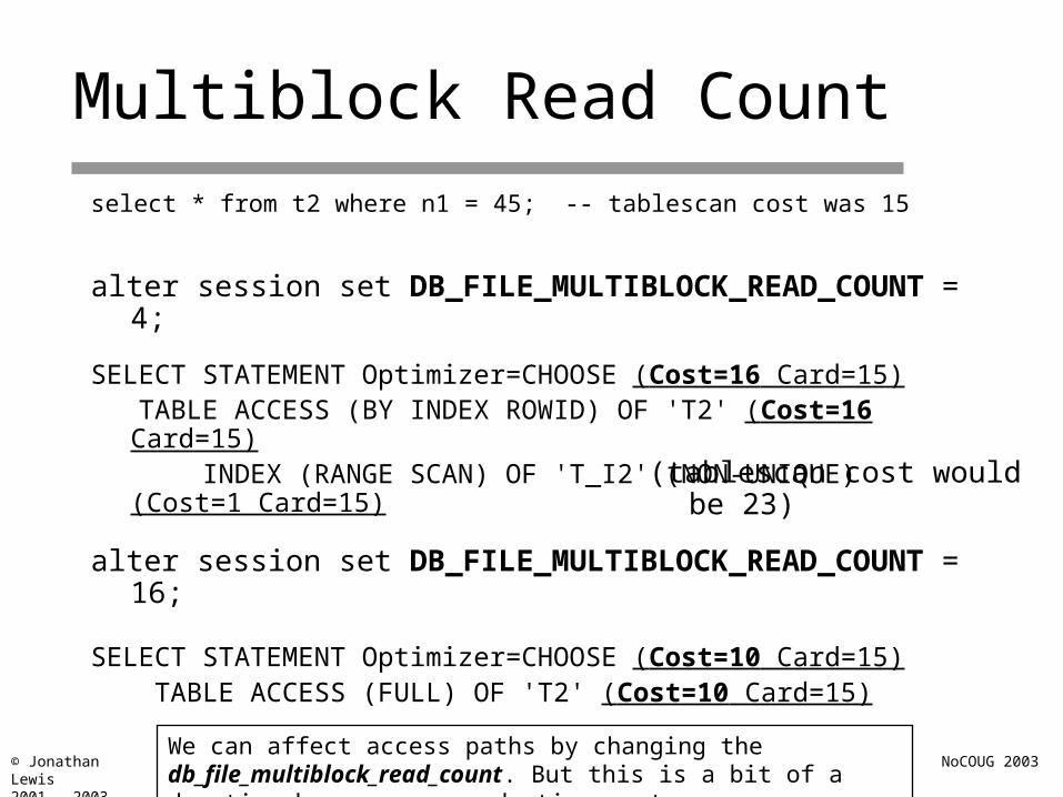
Multiblock Read Count

select * from t2 where n1 = 45; -- tablescan cost was 15

alter session set DB_FILE_MULTIBLOCK_READ_COUNT = 4;


(tablescan cost would be 23)

alter session set DB_FILE_MULTIBLOCK_READ_COUNT = 16;


We can affect access paths by changing the db_file_multiblock_read_count. But this is a bit of a drastic change on a production system.


NoCOUG 2003

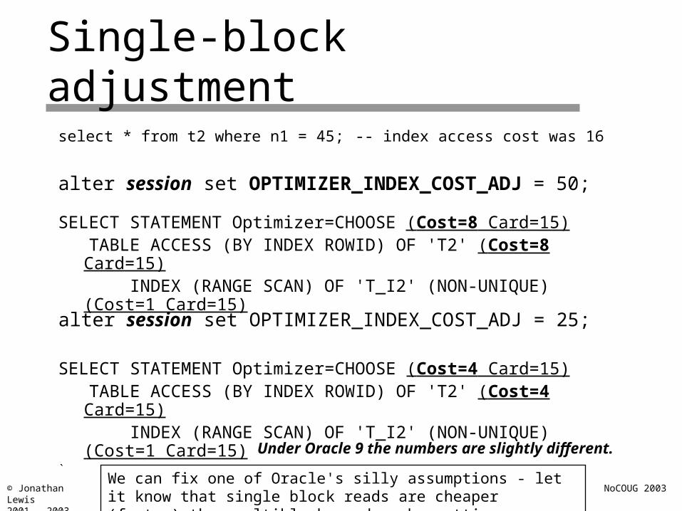
Single-block adjustment

select * from t2 where n1 = 45; -- index access cost was 16

alter session set OPTIMIZER_INDEX_COST_ADJ = 50;



SELECT STATEMENT Optimizer=CHOOSE (Cost=4 Card=15) TABLE ACCESS (BY INDEX ROWID) OF 'T2' (Cost=4 Card=15) INDEX (RANGE SCAN) OF 'T_I2' (NON-UNIQUE) (Cost=1 Card=15)`

Under Oracle 9 the numbers are slightly different.

We can fix one of Oracle's silly assumptions - let it know that single block reads are cheaper (faster) than multiblock reads - by setting a percentage cost


NoCOUG 2003

Single-block adjustment

select event, average_wait from v$system_event -- v$session_event

where event like 'db file s%read';

EVENT AVERAGE_WAITdb file sequential read 1.05db file scattered read 3.72

sequential read time / scattered read time = 1.05/3.72 = 0.28226alter session set optimizer_index_cost_adj = 28;init.ora or login trigger

Tim Gorman (www.evdbt.com) - The search for intelligent life in the CBO.*** but see Garry Robinson: http://www.oracleadvice.com/Tips/optind.htm

The really nice thing about this is that we can set a genuine and realistic cost factor by checking recent, or localised, history. (snapshot v$session_event)


NoCOUG 2003

Join cost-adjustment

select t2.n1, t1.n2from t2,t1where t2.n2 = 45 and t2.n1 = t1.n1;

SELECT STATEMENT (Cost=31 Card=225)

HASH JOIN (Cost=31 Card=25)

TABLE ACCESS (FULL) OF T2 (Cost=15 Card=15)

TABLE ACCESS (FULL) OF T1 (Cost=15 Card=3000)

31 = 15 + 15 + a bit

We can even see the effect of this price fixing in joins. Unhinted, or unfixed, the optimizer chooses a hash join as the cheapest way to our two tables.


NoCOUG 2003

Hash Join (1)

First (smaller)data set

Hashed

Second (larger)data set

The first table is hashed in memory, the second table is used to probe the hash (build) table for matches. In simple cases the cost is easy to calculate.


NoCOUG 2003

Force a nested loop

select /*+ ordered use_nl(t1) index(t1) */t2.n1, t1.n2

from t2,t1where t2.n2 = 45 and t2.n1 = t1.n1;

NESTED LOOPS (Cost=45 Card=225) TABLE ACCESS (FULL) OF T2 (Cost=15, Card=15) TABLE ACCESS (BY ROWID) OF T1(Cost=2,Card=3000) INDEX(RANGE SCAN) OF T_I1(NON-UNIQUE)(Cost=1)

As usual, to investigate why a plan is going wrong, we hint it to make it do what we want - and then look for clues in the resulting cost lines.


NoCOUG 2003

Forced NL cost

alter session set OPTIMIZER_INDEX_COST_ADJ = 100; -- defNESTED LOOPS (Cost=45 Card=225) TABLE ACCESS(FULL) OF T2 (Cost=15, Card=15) TABLE ACCESS(BY ROWID) OF T1(Cost=2, Card=3000) INDEX(RANGE SCAN) OF T_I1(NON-UNIQUE)(Cost=1)

T2 - cost = 15 Estimated rows = 15

For each row from T2 we access T1 by complete key valueT1 - Cost per access = 2

Cost for 15 accesses = 15 x 2 = 30

Total cost of query = cost of T2 + total cost of T1= 15 + 30 = 45

The nested loop algorithm is: for each row in the outer table, use the value in that row to access the inner table - hence the simple formula.


NoCOUG 2003

Nested Loop

T1

T2

The basic arithmetic of the nested loop join is visible in the picture. We do three indexed access into T2, but need the three driving rows from T1 first.


NoCOUG 2003

Nested Loops - recosted


NESTED LOOPS (Cost=30 Card=225) TABLE ACCESS(FULL) OF T2 (Cost=15, Card=15) TABLE ACCESS(BY ROWID) OF T1(Cost=1, Card=3000) INDEX(RANGE SCAN) OF T_I1(NON-UNIQUE)(Cost=1)

T2 - cost = 15 Estimated rows = 15

For each row from T2 we access T1 by complete key valueT1 - Cost per access = 2 x 50% = 1

Cost for 15 accesses = 15 x 1 = 15

Total cost of query = cost of T2 + total cost of T1= 15 + 15 = 30

What happens to the cost when we tell Oracle that single block reads cost half as much as it would otherwise charge ?


NoCOUG 2003

Index Caching (NL only)

Basic nested loop cost (hinted)

NESTED LOOPS (Cost=45 Card=225)TABLE ACCESS (FULL) OF 'T2' (Cost=15, Card=15)TABLE ACCESS (BY INDEX ROWID) OF 'T1' (Cost=2, Card=3000)

INDEX (RANGE SCAN) OF 'T_I1' (NON-UNIQUE) (Cost=1)

alter session set OPTIMIZER_INDEX_CACHING = 100;

NESTED LOOPS (Cost=30 Card=225)TABLE ACCESS (FULL) OF 'T2' (Cost=15, Card=15)TABLE ACCESS (BY INDEX ROWID) OF 'T1' (Cost=1, Card=3000)

INDEX (RANGE SCAN) OF 'T_I1' (NON-UNIQUE)

We can improve silly assumption 2 (every logical I/O is also a physical I/O). Index blocks are often cached. So tell the optimizer how good our cache is.


NoCOUG 2003

Simplifications

• What about the blevel ?

• What about multi-column indexes ?

• What about unbounded ranges ?

• What about unique indexes ?

• What about bitmap indexes ?

This was a visually helpful introduction

This walk-through is intended to give you a gut-feeling of how the optimizer. works. But there are plenty of special cases, and bits of funny arithmetic.


NoCOUG 2003

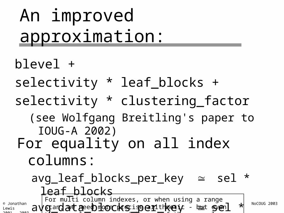
An improved approximation:

blevel +

selectivity * leaf_blocks +

selectivity * clustering_factor (see Wolfgang Breitling's paper to IOUG-A 2002)

For equality on all index columns:avg_leaf_blocks_per_key sel * leaf_blocks

avg_data_blocks_per_key sel * clustering_factor

For multi column indexes, or when using a range scan, we need more precise arithmetic - but even our example was a special case of the general formula


NoCOUG 2003

Adjusted cost:

(

(blevel + selectivity * leaf_blocks) *

(1 - optimizer_index_caching/100)

+

selectivity * clustering_factor

) *

optimizer_index_cost_adj / 100

The formula that Wolfgang Breitling proposed has to be adjusted to handle the two 'fudge factor' parameters. This formula seems to be about right.

Index bit

Table bit


NoCOUG 2003

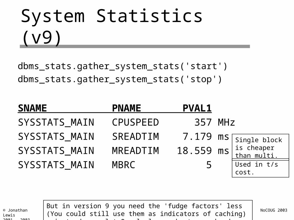
System Statistics (v9)

dbms_stats.gather_system_stats('start')

dbms_stats.gather_system_stats('stop')

SNAME PNAME PVAL1

SYSSTATS_MAIN CPUSPEED 357 MHz

SYSSTATS_MAIN SREADTIM 7.179 ms

SYSSTATS_MAIN MREADTIM 18.559 ms

SYSSTATS_MAIN MBRC 5

Single block is cheaper than multi.

Used in t/s cost.

But in version 9 you need the 'fudge factors' less (You could still use them as indicators of caching) - instead, you let Oracle learn about your hardware


NoCOUG 2003

Conclusions

• Understand your data

• Data distribution is important

• Think about your parameters

• Help Oracle with the truth

• Use system statistics in v9


NoCOUG 2003

Sort / Merge

select

count(t1.v1) ct_v1,

count(t2.v2) ct_v2

from big1 t1, big2 t2

where t2.n2 = t1.n1;

SELECT STATEMENT (choose) Cost (963)SORT (aggregate) MERGE JOIN Cost (963 = 174 + 789) SORT (join) Cost (174) TABLE ACCESS (analyzed) T1 (full) Cost (23) SORT (join) Cost (789) TABLE ACCESS (analyzed) T2 (full) Cost (115)

The cost of a sort-merge equi-join is typically the cost of acquiring each of the two data sets, plus the cost of making sure the two data sets are sorted.


NoCOUG 2003

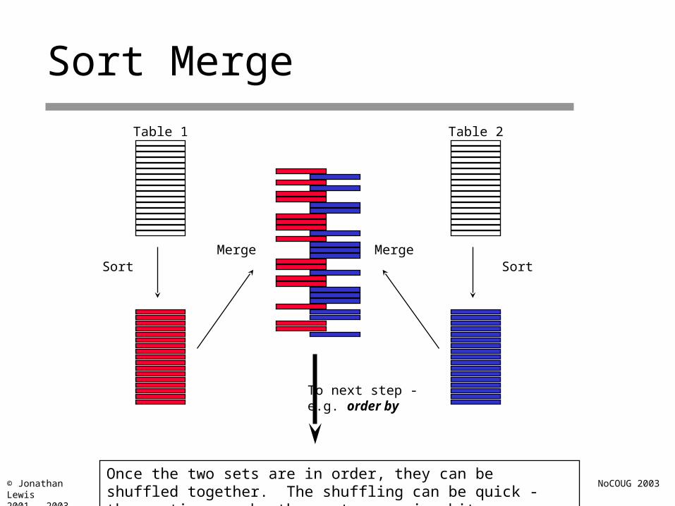
Sort Merge

Table 1

Sort

Table 2

SortMerge Merge

To next step -e.g. order by

Once the two sets are in order, they can be shuffled together. The shuffling can be quick - the sorting may be the most expensive bit.


NoCOUG 2003

In-memory sort

PGA

UGA (will be in SGA for Shared Servers (MTS))

sort_area_retained_size

Sort_area_size - sort_area_retained_sizeTo disc

sort_area_retained_size

In a merge join, even if the first sort completes in memory, it will still dump the excess over sort_area_retained_size to disc. (and so will the second sort)


NoCOUG 2003

Big Sorts

Sort Sort Sort

Merge MergeMerge

A one-pass sort. The data has been read, sorted, and dumped to disc in chunks, then re-read once to be merged into order, and dumped again.


NoCOUG 2003

Huge Sorts

Sort

Merge 1 Merge 2

Merge 3

Multipass sort. After sorting the data in chunks, Oracle was unable to re-read the top of every chunk simultaneously, so we have multiple merge passes.


NoCOUG 2003

Hash Join (1)

First (smaller)data set

Hashed

Second (larger)data set

The first table is hashed in memory, the second table is used to probe the hash (build) table for matches. In simple cases the cost is easy to calculate.


NoCOUG 2003

Hash Join (2)

Small data set

Hashed andpartitioned

Bit mapped

Dump to disc

Big data set

Dumpto disc

If the smaller data set cannot be hashed in memory, it partitioned, mapped, and partly dumped to disc. The larger data set is partitioned in the same way


NoCOUG 2003

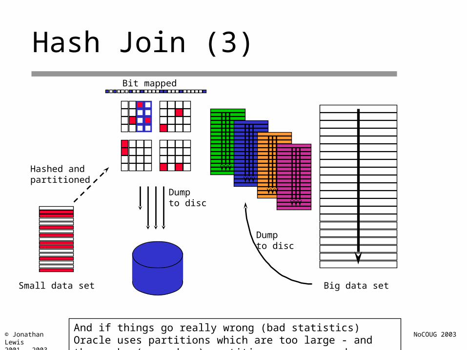
Hash Join (3)

Small data set

Hashed andpartitioned

Bit mapped

Dump to disc

Big data set

Dumpto disc

And if things go really wrong (bad statistics) Oracle uses partitions which are too large - and the probe (secondary) partitions are re-read many times.


NoCOUG 2003

Version 9 approach

v$sysstatSorts, hashes, bitmap creates (v.9)

workarea executions - optimal

The job completed in memory - perfect.

workarea executions - onepass

The job required a dump to disk and single re-read.

workarea executions - multipass

Data was dumped to disc and re-read more than once.

Under Oracle 9, you should be setting workarea_size_policy to true, and use the pga_aggregate_target to something big - the limit per user is 5%

pga_aggregate_target = 500M

worksize_area_policy = auto


NoCOUG 2003

Conclusions 2

• Sort joins have catastrophe points

• Hash joins have catastrophe points

• Work to avoid multi-pass

• pga_aggregate_target helps (v9)

how the cbo works jonathan lewis

Documents