OR I G I N A L AR T I C L E

How to compare sampling designs for mapping?

Alexandre M.J.-C. Wadoux1 | Dick J. Brus2

1Sydney Institute of Agriculture & Schoolof Life and Environmental Sciences, TheUniversity of Sydney, Sydney, Australia2Biometris, Wageningen University andResearch, Wageningen, The Netherlands

CorrespondenceDick J. Brus, Droevendaalsesteeg1, 6708 PB Wageningen, The Netherlands.Email: dick.brus@wur.nl

Funding informationNo funding has been received to carry outthis study.

Abstract

If a map is constructed through prediction with a statistical or non-statistical

model, the sampling design used for selecting the sample on which the model is

fitted plays a key role in the final map accuracy. Several sampling designs are avail-

able for selecting these calibration samples. Commonly, sampling designs for map-

ping are compared in real-world case studies by selecting just one sample for each

of the sampling designs under study. In this study, we show that sampling designs

for mapping are better compared on the basis of the distribution of the map quality

indices over repeated selection of the calibration sample. In practice this is only fea-

sible by subsampling a large dataset representing the population of interest, or by

selecting calibration samples from a map depicting the study variable. This is illus-

trated with two real-world case studies. In the first case study a quantitative vari-

able, soil organic carbon, is mapped by kriging with an external drift in France,

whereas in the second case a categorical variable, land cover, is mapped by random

forest in a region in France. The performance of two sampling designs for mapping

are compared: simple random sampling and conditioned Latin hypercube sam-

pling, at various sample sizes. We show that in both case studies the sampling dis-

tributions of map quality indices obtained with the two sampling design types, for

a given sample size, show large variation and largely overlap. This shows that

when comparing sampling designs for mapping on the basis of a single sample

selected per design, there is a serious risk of an incidental result.

Highlights

• We provide a method to compare sampling designs for mapping.

• Random designs for selecting calibration samples should be compared on

the basis of the sampling distribution of the map quality indices.

KEYWORD S

Kriging, machine learning, pedometrics, random forest, soil sampling, validation

1 | INTRODUCTION

In recent years, there has been an increase in digital soilmapping (DSM) activities (Arrouays, Lagacherie, &Hartemink, 2017). Digital maps of soil properties are

predicted from a geostatistical model or machine learningalgorithm fitted on a sample of units selected from the areato be mapped. Because the sample is the basis for mapping,its size and spatial pattern play a key role in the resulting soilmap accuracy. Hereafter a sample used for fitting a statistical

Received: 20 November 2019 Revised: 24 March 2020 Accepted: 25 March 2020

DOI: 10.1111/ejss.12962

This is an open access article under the terms of the Creative Commons Attribution-NonCommercial License, which permits use, distribution and reproduction in any

medium, provided the original work is properly cited and is not used for commercial purposes.

© 2020 The Authors. European Journal of Soil Science published by John Wiley & Sons Ltd on behalf of British Society of Soil Science.

Eur J Soil Sci. 2020;1–12. wileyonlinelibrary.com/journal/ejss 1

model or training a machine learning algorithm is referred toas a calibration sample. Sampling designs used for selectingcalibration samples that are subsequently used for mappingare referred to as sampling designs for mapping.

In the statistical and DSM literature, several solutionshave been proposed to select the sampling locations forfitting or training a model and mapping. For an overviewof common sampling designs for soil mapping, we redirectreaders to De Gruijter, Brus, Bierkens, and Knotters (2006)and Brus (2019). The large number of available samplingdesigns has logically led to studies comparing the effectsampling designs have on the resulting mapping accuracy.Schmidt et al. (2014) compared three different samplingdesigns and their effect on the mapping accuracy of fivesoil properties at field scale. In this study, with each designa single sample is collected in the field and used for modelfitting and prediction. Besides, to validate a map obtainedwith the calibration sample of a given design, the calibra-tion samples of the other designs were used, so that noreliable conclusions can be drawn from this study. Simi-larly, Werbylo and Niemann (2014) evaluated stratifiedrandom and conditioned Latin hypercube samplingdesigns for soil moisture downscaling at three local-scalecatchments. The selection of samples with the designsunder study is repeated 100 times and compared using theaveraged values of the Nash-Sutcliffe coefficient of effi-ciency between the observed and predicted downscaledpatterns. The authors found mixed results, stratified ran-dom sampling being more efficient than conditioned Latinhypercube sampling for small sample sizes (fewer than30 units) while it was the opposite for larger sample sizes.

Repeated selection of samples with a probability sam-pling design leads to different samples and different esti-mates of the population mean or total. This is also the casefor commonly used sampling designs for mapping, such asspatial coverage sampling supplemented by short distancepoints (Lark & Marchant, 2018), feature space coveragesampling (Brus, 2019), conditioned Latin hypercube sam-pling (Minasny & McBratney, 2006) and model-baseddesigns for mapping, such as the designs proposed by VanGroenigen (2000), Brus and Heuvelink (2007), Marchantand Lark (2007) or Wadoux, Marchant, and Lark (2019),among others. In all these sampling designs a randomnumber generator is used at some stage in the selectionprocess. In the design proposed by Lark and March-ant (2018) the points of the supplemental sample areselected randomly at a fixed but random distance from a(random) subset of the spatial coverage sample. In featurespace coverage sampling, k-means is used to minimize acriterion. The initial clustering is chosen randomly. In con-ditioned Latin hypercube sampling and model-based sam-pling designs for mapping a criterion is minimized bysimulated annealing in which proposal samples are

generated by random selection of one point of the currentsample and shifting it to a random selected location. Therandomness in the selection of the locations of a calibrationsample may have an impact on the resulting map accuracy.This has as yet been disregarded in previous studies evalu-ating and comparing sampling designs for mapping.

The aim of our paper is to show the importance ofrepeated selection of calibration samples from real-world orsimulated populations when comparing sampling designsfor mapping in which randomness is involved. Similar tocomparing probability sampling designs for estimating thepopulation mean on the basis of the sampling distribution ofthe estimated population mean, not just on the basis of theerror obtained with a single probability sample, samplingdesigns should be compared on the basis of the distributionof map quality indices over repeated selection of samples.We illustrate this with two real-world case studies, one for aquantitative variable and one for a categorical variable. Wecompare simple random sampling (SRS) and conditionedLatin hypercube sampling (cLHS) at various sample sizes.

2 | THEORY AND METHODS

2.1 | Map quality indices

A wide variety of map quality indices is available(Congalton, 1991; Janssen & Heuberger, 1995;Stehman, 1997). Commonly used quality indices of contin-uous maps are the population means of the prediction error(ME) and of the squared prediction error (MSE), defined as:

ME=1N

XNi=1

ɛ sið Þ, ð1Þ

MSE=1N

XNi=1

ɛ sið Þ2, ð2Þ

where ɛ sið Þ= z sið Þ−z sið Þ is the error, in which z and zdenote the measured and predicted soil variable at loca-tion si, i = 1, …, N, respectively, and N is the total numberof population units.

The quality of categorical maps is commonly quanti-fied by the overall accuracy (OA), defined as:

OA=1N

XNi=1

a sið Þ, ð3Þ

where a(si) is an indicator defined as follows:

a sið Þ= 1 c sið Þ= c sið Þ0 c sið Þ 6¼ c sið Þ

�, ð4Þ

2 WADOUX AND BRUS

with c sið Þ the predicted class for population unit i andc sið Þ the true class for that unit. For infinite populations,the summation in Equations (1)–(3) is approximated by anintegral.

2.2 | Evaluation of sampling designs formapping

We propose to evaluate random designs for mapping onthe basis of the sampling distribution of map quality indi-ces: fp(ME), fp(MSE) and fp(OA). The subscript p refers toa sampling design for selecting the calibration samples.Of special interest are the expectation and variance ofthese distributions. The expectation and variance of theMSE are defined as:

Ep MSEð Þ=XSMSE Sð Þ p Sð Þ, ð5Þ

Vp MSEð Þ=XS

MSEðSÞ−EpðMSEÞ� �2p Sð Þ, ð6Þ

with MSE Sð Þ being the population MSE for calibrationsample S and p Sð Þ the selection probability of sample S .By replacing MSE in Equations (5) and (6) by ME andOA we obtain the definition of the expectation and vari-ance of the mean error and overall accuracy, respectively.Note that Ep(MSE) = Vp(ME)+ {Ep(ME)}2. Although aninfinite number of samples S can be selected, in practicewe proceed by selecting a large but finite number of sam-ples from the population.

These are sampling distributions of the overall mapquality. For mapping we propose to evaluate the sam-pling designs also on the basis of the sampling distribu-tions for individual units (points), fp{ɛ(si)}, fp{ɛ

2(si)} andfp{a(si)}, i = 1, …, N. Maps of the expectation and vari-ance of these point-wise distributions may reveal perfor-mance characteristics that remain undiscovered whenlooking at the distribution of overall map quality indicesonly. The expectation and variance of the squared errorare defined as:

Ep ɛ2i� �

=XSɛ2i Sð Þ p Sð Þ, ð7Þ

Vp ɛ2i� �

=XS

ɛ2i Sð Þ−Ep ɛ2i� �� �2

p Sð Þ, ð8Þ

with ɛi = ɛ sið Þ. The expectation and variance of the errorsand accuracy indicators for individual units are obtainedby replacing ɛ2i in Equations 7 and 8 by ɛi and ai, respec-tively. Note that Ep ɛ2i

� �=Vp ɛið Þ+ Ep ɛið Þ� �2

.

The sampling distributions are approximated by inde-pendent selection of a large number, say R, of calibrationsamples. The expectation and variance of the populationmean of the quality indices and of the point-wise mapquality indices are estimated by the average and varianceacross these R calibration samples. In the case study withthe continuous variable R = 1,000, whereas R = 400 inthe case study for the categorical variable. For thesquared errors the estimators are:

Ep MSEð Þ= 1R

XRS=1

MSE Sð Þ, ð9Þ

Vp MSEð Þ= 1R−1

XRS=1

MSE Sð Þ− 1R

XRS=1

MSE Sð Þ !2

, ð10Þ

Ep ɛ2i� �

=1R

XRS=1

ɛ2i Sð Þ, ð11Þ

Vp ɛ2i� �

=1

R−1

XRS=1

ɛ2i Sð Þ− 1R

XRS=1

ɛ2i Sð Þ !2

: ð12Þ

To avoid confusion we would like to stress that in thispaper the indices to quantify the quality of a map are notdefined across realizations of a model used for prediction(mapping), but across realizations of a sampling designused to select a calibration sample for mapping, as indi-cated by the subscript p in fp, Ep and Vp. This is also thecase when a statistical model is used for prediction (map-ping), such as in the second case study hereafter, inwhich kriging with an external drift is used. This impliesthat, given a calibration sample, the prediction errors atpoints, as well as the population mean of the (squared)errors are fixed quantities, not random variables. By con-sidering all calibration samples that can be selected bythe sampling design, both the point-wise predictionerrors, as well as the population mean of the errorsbecome random quantities. The distributions of theserandom quantities are not model distributions, but sam-pling distributions, as indicated by the subscript p in fp.In a model-based approach the statistical inference isconditioned on the calibration sample. No other samplesthan the one actually selected are considered. Random-ness is introduced via the statistical model that is used inthe inference, so that the prediction errors at points andthe population mean of the (squared) errors become ran-dom variables, despite the conditioning on the calibrationsample. The distributions of these random variables aremodel distributions, i.e., distributions defined over allpossible realizations of the statistical model, which are

WADOUX AND BRUS 3

fundamentally different from sampling distributions,which we considered in this paper.

2.3 | Sampling designs for mapping

Two sampling designs for mapping are compared, condi-tioned Latin hypercube (cLHS) and simple random sam-pling (SRS).

Conditioned Latin hypercube sampling (cLHS,Minasny and McBratney (2006)) is an adaptation of theexperimental design Latin hypercube sampling (LHS)for observational research. The adaptation is neededbecause not all combinations of factor levels may be rep-resented in the population of interest. In cLHS the factorlevels are marginal strata of equal size, i.e., with equalnumber of pixels. In total, there are nc marginal strata,with n the total sample size and c the number ofcovariates. With continuous covariates only, a cLHS isselected by minimizing a weighted sum of two compo-nents. The first component is the sum over all marginalstrata of the absolute difference of the marginal stratumsample size and the targeted sample size of one unit.The second component is the sum of the absolute differ-ence of the entries of the sample correlation matrix andpopulation correlation matrix. So in cLHS the marginaldistributions of the covariates are uniformly covered,while accounting for the correlation between thecovariates.

Simple random sampling is the simplest form of sam-pling design. It does not require any prior knowledge onthe spatial variation and does not exploit environmentalcovariates. In SRS, each unit in the population has equalprobability of being selected and the units are selectedindependently from each other.

3 | CASE STUDIES

3.1 | Mapping topsoil organic carboncontent

We used the measurements collected over France withinthe framework of the European Land Use/Cover Areaframe Statistical Survey (LUCAS). The database is com-posed of N = 2,947 georeferenced values of the topsoil(0–30 cm) organic carbon (SOC, in g kg−1) as measuredby an automated vario MAX CN analyzer (ElementarAnalysensysteme GmbH, Germany) (Tóth, Jones, &Montanarella, 2013). The SOC values were log-transformed to correct for the highly skewed (skew-ness = 6.12) distribution. In this study, the N = 2,947 log-transformed SOC values are considered as our population

of interest. In other words, we ignore that the LUCASdata are a sample of another area of interest (France). Inaddition, we collected five environmental covariates formodelling the mean (spatial trend). The covariates wereeither resampled using bilinear interpolation or aggre-gated to conform with a resolution of 1 km × 1 km, andtheir value was extracted to the location of the N = 2,947LUCAS sampling locations. The covariates were theLandsat Band 3 (red) for the year 2014, the long-termaveraged mean annual surface temperature (daytime)MODIS (in degrees Kelvin), the total annual precipitation(in mm/year), the elevation (in metre) and the multi-resolution index of valley bottom flatness (MRVBF) inmetre × 100.

In this study, predictions of the topsoil log-transformed organic carbon were obtained by krigingwith an external drift (Webster & Oliver, 2007). We fittedan exponential variogram model to the residuals of thesoil property using ordinary least square in an automaticfitting and prediction procedure (Hiemstra, 2015). Thelinear trend was composed of the covariates describedabove.

For each calibration sample the MSE was computedby using the calibrated model to predict log-transformedorganic carbon for all LUCAS points, including the pointsused for calibrating the model.

3.2 | Land cover classification

In the second case study, we used the CORINE LandCover (CLC) inventory map updated in 2018 (Feranec,Soukup, Hazeu, & Jaffrain, 2016) as our variable of inter-est. The CLC map is a categorical map of 44 classes cover-ing the whole of Europe with grid cells of 100 m × 100 mresolution. We used a subset of 39,151 km2 of this map,covering the French region Centre-Val de Loire. In thisregional area, 26 out of the 44 land cover classes are pre-sent. To speed up computation, we further selected alarge sub-grid of the CLC map with a spacing of 400 m,resulting in N = 247,061 grid points. This large subsam-ple is used as a basis to collect the calibration samples. Aset of 12 environmental covariates were used as predictorin the model. The covariates were the water table depthin metre, the average soil and sedimentary-deposit thick-ness in metre, the Landsat Band 4 (NIR) for the year2014, the Landsat Band 3 (red) for the year 2014, theLandsat Band 5 (SWIR) for year 2014, the Landsat Band7 (SWIR) for year 2014, the long-term averaged meanannual surface temperature (daytime) MODIS(in Kelvin), the total annual precipitation (in mm/year),the elevation (in metre), the terrain slope in radian× 100, SAGA Wetness Index in metre × 10 and the

4 WADOUX AND BRUS

multiresolution index of valley bottom flatness (MRVBF)in metre × 100.

For categorical variables, predictions were made by arandom forest (Breiman, 2001) model using thecovariates listed above. We used the implementation pro-vided by Wright and Ziegler (2017), and set the tuningparameters nodesize and mtry to their default values andntree to 1,000.

4 | RESULTS

4.1 | Quality of organic carbon map

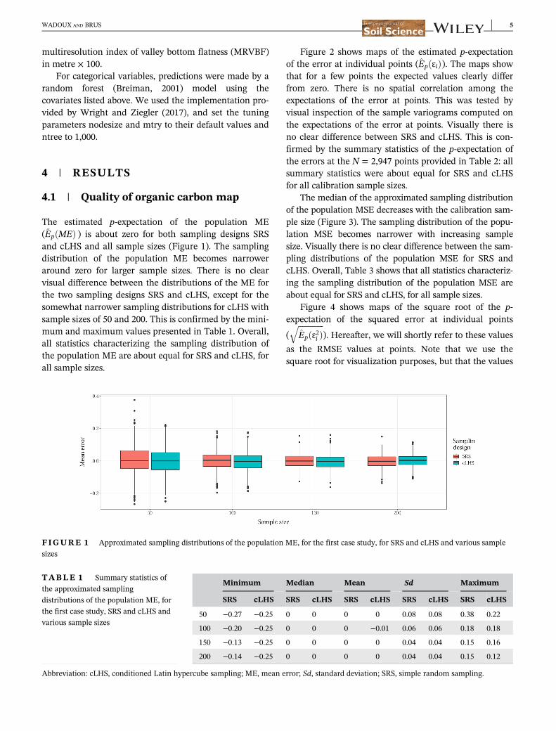
The estimated p-expectation of the population ME(Ep MEð Þ ) is about zero for both sampling designs SRSand cLHS and all sample sizes (Figure 1). The samplingdistribution of the population ME becomes narroweraround zero for larger sample sizes. There is no clearvisual difference between the distributions of the ME forthe two sampling designs SRS and cLHS, except for thesomewhat narrower sampling distributions for cLHS withsample sizes of 50 and 200. This is confirmed by the mini-mum and maximum values presented in Table 1. Overall,all statistics characterizing the sampling distribution ofthe population ME are about equal for SRS and cLHS, forall sample sizes.

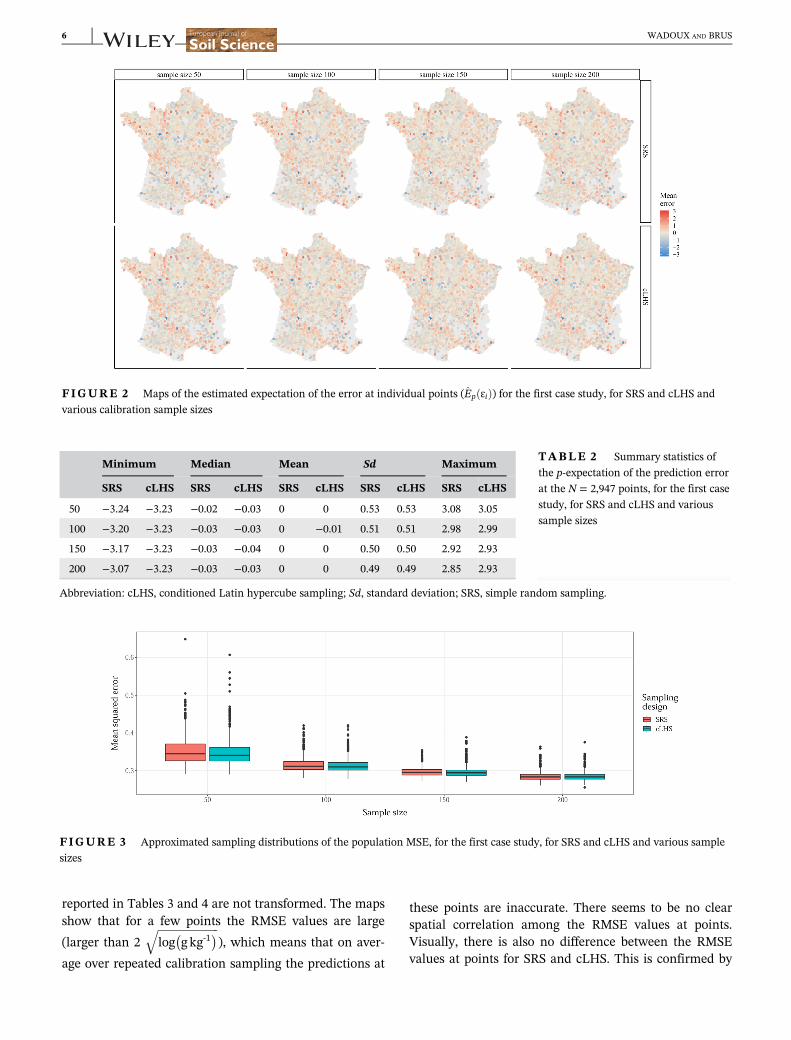
Figure 2 shows maps of the estimated p-expectationof the error at individual points (Ep ɛið Þ). The maps showthat for a few points the expected values clearly differfrom zero. There is no spatial correlation among theexpectations of the error at points. This was tested byvisual inspection of the sample variograms computed onthe expectations of the error at points. Visually there isno clear difference between SRS and cLHS. This is con-firmed by the summary statistics of the p-expectation ofthe errors at the N = 2,947 points provided in Table 2: allsummary statistics were about equal for SRS and cLHSfor all calibration sample sizes.

The median of the approximated sampling distributionof the population MSE decreases with the calibration sam-ple size (Figure 3). The sampling distribution of the popu-lation MSE becomes narrower with increasing samplesize. Visually there is no clear difference between the sam-pling distributions of the population MSE for SRS andcLHS. Overall, Table 3 shows that all statistics characteriz-ing the sampling distribution of the population MSE areabout equal for SRS and cLHS, for all sample sizes.

Figure 4 shows maps of the square root of the p-expectation of the squared error at individual points

(ffiffiffiffiffiffiffiffiffiffiffiffiffiEp ɛ2ið Þ

q). Hereafter, we will shortly refer to these values

as the RMSE values at points. Note that we use thesquare root for visualization purposes, but that the values

FIGURE 1 Approximated sampling distributions of the population ME, for the first case study, for SRS and cLHS and various sample

sizes

TABLE 1 Summary statistics of

the approximated sampling

distributions of the population ME, for

the first case study, SRS and cLHS and

various sample sizes

Minimum Median Mean Sd Maximum

SRS cLHS SRS cLHS SRS cLHS SRS cLHS SRS cLHS

50 −0.27 −0.25 0 0 0 0 0.08 0.08 0.38 0.22

100 −0.20 −0.25 0 0 0 −0.01 0.06 0.06 0.18 0.18

150 −0.13 −0.25 0 0 0 0 0.04 0.04 0.15 0.16

200 −0.14 −0.25 0 0 0 0 0.04 0.04 0.15 0.12

Abbreviation: cLHS, conditioned Latin hypercube sampling; ME, mean error; Sd, standard deviation; SRS, simple random sampling.

WADOUX AND BRUS 5

reported in Tables 3 and 4 are not transformed. The mapsshow that for a few points the RMSE values are large

(larger than 2ffiffiffiffiffiffiffiffiffiffiffiffiffiffiffiffiffiffiffiffiffiffilog g kg-1� �q

), which means that on aver-

age over repeated calibration sampling the predictions at

these points are inaccurate. There seems to be no clearspatial correlation among the RMSE values at points.Visually, there is also no difference between the RMSEvalues at points for SRS and cLHS. This is confirmed by

FIGURE 2 Maps of the estimated expectation of the error at individual points (Ep ɛið Þ) for the first case study, for SRS and cLHS and

various calibration sample sizes

TABLE 2 Summary statistics of

the p-expectation of the prediction error

at the N = 2,947 points, for the first case

study, for SRS and cLHS and various

sample sizes

Minimum Median Mean Sd Maximum

SRS cLHS SRS cLHS SRS cLHS SRS cLHS SRS cLHS

50 −3.24 −3.23 −0.02 −0.03 0 0 0.53 0.53 3.08 3.05

100 −3.20 −3.23 −0.03 −0.03 0 −0.01 0.51 0.51 2.98 2.99

150 −3.17 −3.23 −0.03 −0.04 0 0 0.50 0.50 2.92 2.93

200 −3.07 −3.23 −0.03 −0.03 0 0 0.49 0.49 2.85 2.93

Abbreviation: cLHS, conditioned Latin hypercube sampling; Sd, standard deviation; SRS, simple random sampling.

FIGURE 3 Approximated sampling distributions of the population MSE, for the first case study, for SRS and cLHS and various sample

sizes

6 WADOUX AND BRUS

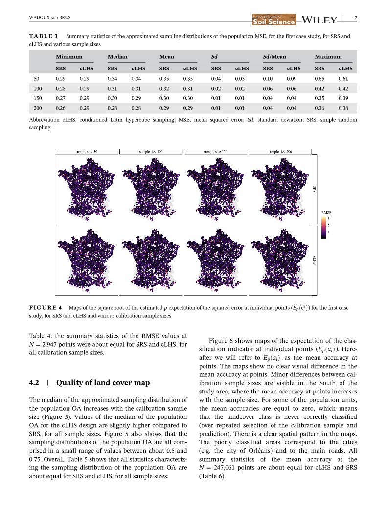
Table 4: the summary statistics of the RMSE values atN = 2,947 points were about equal for SRS and cLHS, forall calibration sample sizes.

4.2 | Quality of land cover map

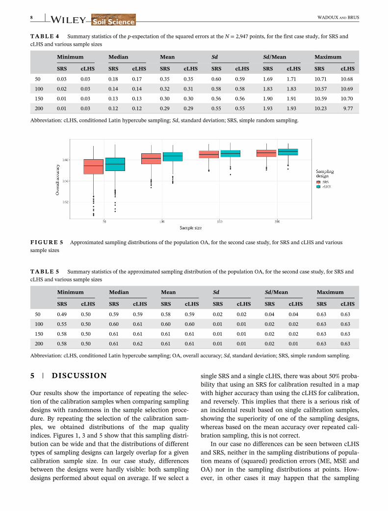
The median of the approximated sampling distribution ofthe population OA increases with the calibration samplesize (Figure 5). Values of the median of the populationOA for the cLHS design are slightly higher compared toSRS, for all sample sizes. Figure 5 also shows that thesampling distributions of the population OA are all com-prised in a small range of values between about 0.5 and0.75. Overall, Table 5 shows that all statistics characteriz-ing the sampling distribution of the population OA areabout equal for SRS and cLHS, for all sample sizes.

Figure 6 shows maps of the expectation of the clas-sification indicator at individual points (Ep aið Þ). Here-after we will refer to Ep aið Þ as the mean accuracy atpoints. The maps show no clear visual difference in themean accuracy at points. Minor differences between cal-ibration sample sizes are visible in the South of thestudy area, where the mean accuracy at points increaseswith the sample size. For some of the population units,the mean accuracies are equal to zero, which meansthat the landcover class is never correctly classified(over repeated selection of the calibration sample andprediction). There is a clear spatial pattern in the maps.The poorly classified areas correspond to the cities(e.g. the city of Orléans) and to the main roads. Allsummary statistics of the mean accuracy at theN = 247,061 points are about equal for cLHS and SRS(Table 6).

TABLE 3 Summary statistics of the approximated sampling distributions of the population MSE, for the first case study, for SRS and

cLHS and various sample sizes

Minimum Median Mean Sd Sd/Mean Maximum

SRS cLHS SRS cLHS SRS cLHS SRS cLHS SRS cLHS SRS cLHS

50 0.29 0.29 0.34 0.34 0.35 0.35 0.04 0.03 0.10 0.09 0.65 0.61

100 0.28 0.29 0.31 0.31 0.32 0.31 0.02 0.02 0.06 0.06 0.42 0.42

150 0.27 0.29 0.30 0.29 0.30 0.30 0.01 0.01 0.04 0.04 0.35 0.39

200 0.26 0.29 0.28 0.28 0.29 0.29 0.01 0.01 0.04 0.04 0.36 0.38

Abbreviation cLHS, conditioned Latin hypercube sampling; MSE, mean squared error; Sd, standard deviation; SRS, simple randomsampling.

FIGURE 4 Maps of the square root of the estimated p-expectation of the squared error at individual points (Ep ɛ2i� �

) for the first case

study, for SRS and cLHS and various calibration sample sizes

WADOUX AND BRUS 7

5 | DISCUSSION

Our results show the importance of repeating the selec-tion of the calibration samples when comparing samplingdesigns with randomness in the sample selection proce-dure. By repeating the selection of the calibration sam-ples, we obtained distributions of the map qualityindices. Figures 1, 3 and 5 show that this sampling distri-bution can be wide and that the distributions of differenttypes of sampling designs can largely overlap for a givencalibration sample size. In our case study, differencesbetween the designs were hardly visible: both samplingdesigns performed about equal on average. If we select a

single SRS and a single cLHS, there was about 50% proba-bility that using an SRS for calibration resulted in a mapwith higher accuracy than using the cLHS for calibration,and reversely. This implies that there is a serious risk ofan incidental result based on single calibration samples,showing the superiority of one of the sampling designs,whereas based on the mean accuracy over repeated cali-bration sampling, this is not correct.

In our case no differences can be seen between cLHSand SRS, neither in the sampling distributions of popula-tion means of (squared) prediction errors (ME, MSE andOA) nor in the sampling distributions at points. How-ever, in other cases it may happen that the sampling

TABLE 4 Summary statistics of the p-expectation of the squared errors at the N = 2,947 points, for the first case study, for SRS and

cLHS and various sample sizes

Minimum Median Mean Sd Sd/Mean Maximum

SRS cLHS SRS cLHS SRS cLHS SRS cLHS SRS cLHS SRS cLHS

50 0.03 0.03 0.18 0.17 0.35 0.35 0.60 0.59 1.69 1.71 10.71 10.68

100 0.02 0.03 0.14 0.14 0.32 0.31 0.58 0.58 1.83 1.83 10.57 10.69

150 0.01 0.03 0.13 0.13 0.30 0.30 0.56 0.56 1.90 1.91 10.59 10.70

200 0.01 0.03 0.12 0.12 0.29 0.29 0.55 0.55 1.93 1.93 10.23 9.77

Abbreviation: cLHS, conditioned Latin hypercube sampling; Sd, standard deviation; SRS, simple random sampling.

FIGURE 5 Approximated sampling distributions of the population OA, for the second case study, for SRS and cLHS and various

sample sizes

TABLE 5 Summary statistics of the approximated sampling distribution of the population OA, for the second case study, for SRS and

cLHS and various sample sizes

Minimum Median Mean Sd Sd/Mean Maximum

SRS cLHS SRS cLHS SRS cLHS SRS cLHS SRS cLHS SRS cLHS

50 0.49 0.50 0.59 0.59 0.58 0.59 0.02 0.02 0.04 0.04 0.63 0.63

100 0.55 0.50 0.60 0.61 0.60 0.60 0.01 0.01 0.02 0.02 0.63 0.63

150 0.58 0.50 0.61 0.61 0.61 0.61 0.01 0.01 0.02 0.02 0.63 0.63

200 0.58 0.50 0.61 0.62 0.61 0.61 0.01 0.01 0.02 0.01 0.63 0.63

Abbreviation: cLHS, conditioned Latin hypercube sampling; OA, overall accuracy; Sd, standard deviation; SRS, simple random sampling.

8 WADOUX AND BRUS

distributions of overall map quality indices such as OAand MSE are about equal, but not so the distributions atpoints. For instance, when the p-expectation of the popu-lation ME is close to zero, the p-expectation of the errorat points still can largely differ from zero as long as posi-tive and negative errors are in balance. A samplingdesign with a p-expectation of ME close to zero andbesides small values for the p-expectation of the point-wise errors, is to be preferred over a sampling design withlarger values for the p-expectation of the point-wiseerrors.

Similarly, two designs with about equal values for thep-expectation of the population MSE can be quite differ-ent when looking at the spatial variation of thep-expectation of the squared errors at points.

In our case studies, SRS and cLHS were equivalent interms of map accuracy. Several studies (e.g., Castro-Franco, Costa, Peralta, & Aparicio, 2015; Chu, Lin,

Jang, & Chang, 2010; Contreras, Ballari, De Bruin, &Samaniego, 2019; Domenech, Castro-Franco, Costa, &Amiotti, 2017; Schmidt et al., 2014) concluded that cLHSin combination with kriging or random forest for map-ping gave the most accurate prediction. These studiespromote the use of cLHS as an effective sampling designfor mapping. We emphasize that the results of the studiespreviously cited are possible outcomes (as shown by Fig-ures 3 and 5), but, their conclusion on a sampling designperforming better than another is potentially incidentalbecause the selection of the calibration sample was notrepeated. Our case studies, conversely, confirm someearlier conclusions made by Worsham, Markewitz,Nibbelink, and West (2012) and later Wadoux, Brus, andHeuvelink (2019) and Ma, Brus, Zhu, Zhang, andScholten (2020). Worsham et al. (2012) compared SRS,stratified random sampling and cLHS for selecting cali-bration samples on the basis of the root mean squared

FIGURE 6 Maps of the estimated mean accuracy at points of the second case study, for both SRS and cLHS and different calibration

sample sizes

TABLE 6 Summary statistics of the estimated mean accuracy (Ep aið Þ) at the N = 247,061 points, for the second case study, for SRS and

cLHS and various sample sizes

Minimum Median Mean Sd Sd/Mean Maximum

SRS cLHS SRS cLHS SRS cLHS SRS cLHS SRS cLHS SRS cLHS

50 0 0 0.73 0.75 0.58 0.59 0.41 0.41 0.69 0.69 1 1

100 0 0 0.80 0.82 0.60 0.60 0.41 0.41 0.69 0.69 1 1

150 0 0 0.84 0.85 0.61 0.61 0.42 0.42 0.69 0.69 1 1

200 0 0 0.85 0.86 0.61 0.61 0.42 0.42 0.69 0.68 1 1

Abbreviation: cLHS, conditioned Latin hypercube sampling; Sd, standard deviation; SRS, simple random sampling.

WADOUX AND BRUS 9

error of the mapped soil C content over a 12ha field. Byrepeating the selection of the calibration sample 10 timesfrom the population, they showed that while there was aclear advantage in terms of resulting map accuracy(RMSE) for stratified random sampling and cLHS overSRS, the authors did not find an apparent improvementwhen using cLHS over stratified random sampling. Thiswas further confirmed by Wadoux et al. (2019) and Maet al. (2020) when comparing sampling designs for map-ping with random forest. There is need for furtherresearch in this direction.

In practice we do not have exhaustive knowledge ofthe population values, so that the map accuracy obtainedwith a given calibration sample must be estimated from aprobability sample. The validation sampling error con-tributes to the total variance of the map quality index.We estimated this contribution by estimating the expecta-tion over repeated calibration sampling of the validationsampling variance of the estimated map quality index.The results (reported in the Appendix) show that the con-tribution of the validation sampling error to the total var-iance of the map quality index was large in both casestudies, even with a validation sample size of 200. Inmost DSM studies, the validation sample size is limited,and often much smaller than the calibration sample size.One can then expect that the uncertainty about the mapaccuracy is large. In these cases, it is best to compute con-fidence intervals of the map quality indices (ME, MSEand OA) and to test whether differences in the estimatedmap quality indices are significant using a paired t-test orWilcoxon signed-rank test. This is only feasible when thevalidation locations are selected by probability sampling(Brus, Kempen, & Heuvelink, 2011). Since in practice theobjective is to obtain a map (not to estimate the mapquality index) and it is likely that an additional samplingeffort is integrated into the calibration sample rather thanused for validation, we did not pursue any further in thisdirection.

5.1 | Various types of study to comparedesigns for mapping

We emphasize the need for various types of study to com-pare sampling designs for mapping: (a) real-world casestudies, (b) studies where a very large dataset is treated asthe population of interest, (c) studies in which a map ofthe study variable is treated as error free so that we haveexhaustive knowledge of the study variable, and(d) geostatistical simulation studies.

Real-world case studies are by far the most commonapproaches to date. In a real-world case study, the cali-bration samples of the sampling designs under study are

collected in a study area, used to calibrate a model, andcompared based on some map quality indices. An advan-tage of these studies is that the data are real-world datathat generally do not perfectly behave according to ourprobability models. An important disadvantage is that ingeneral we cannot afford to repeat the selection of cali-bration samples, so our conclusion about the relative per-formance of sampling designs for mapping is necessarilyconditioned on the two samples selected. Another disad-vantage is that the map accuracy is unknown and mustbe estimated from a probability sample.

Similar to the real-world case studies, an advantage ofstudies where a large dataset is treated as the populationof interest is that the data are real-world data. Anotheradvantage is that the selection of calibration samples canbe repeated, so that the sampling distribution of the mapquality index can be assessed, and more general conclu-sions about the relative performance of sampling designsfor mapping can be drawn. The main drawback is thatthe population is a sample of the true population of inter-est. The dataset must be sufficiently large to cover thecharacteristics of the true population. Also, the samplingfraction of the calibration sample must be very small, sothat approximately errorless estimates of the map qualityindex can be obtained.

When using a map as reality, we either have a verylarge but finite population of raster cells or an infinitepopulation (polygon map). As a consequence, selection ofcalibration samples can be repeated, and the map qualitycan be assessed from a very large validation sample, sothat the computed map quality index can be treated aserrorless. However, we treat the predictions as depictedon the map as errorless predictions. But actually we arecomparing two predictions, one of which is treated as theground truth. The map quality indices are only realisticestimates of the map accuracy in real-world surveys ofthe area depicted on the map when the quality of themap used as reality is very high. It is hard to say whetherthe computed map quality index over- or under-estimatesthe map quality with real-world surveys. Under theassumption that the systematic error in the map qualityindex is equal for the sampling designs under study, thistype of study still may give valuable information aboutthe relative performance of sampling designs for mappingbased on the sampling distribution.

In geostatistical simulation studies, a large number ofspatial populations can be generated using variousmodels of spatial variation. With this type of study, thesampling distributions of the model expectation of themap quality index can be computed for the samplingdesigns under study. This gives insight into the relativeperformance of sampling designs for mapping under vari-ous models of spatial variation.

10 WADOUX AND BRUS

We recommend that, before a novel sampling designfor selecting calibration samples is published, the perfor-mance of this novel design is compared with existingsampling designs, not only on the basis of the map accu-racies obtained with a single sample per design, but pref-erably on the basis of the sampling distributions of themap accuracy over repeated calibration sampling. This isto avoid that a novel design is embraced by many scien-tists, and after many applications it appears that thenovel design performed worse than existing designs.

The alternative to these empirical studies is to reasonfrom theory that the proposed design performs betterthan existing designs. For instance, in an experimentaldesign with numerous factors and many levels for eachfactor, Latin hypercube sampling is more efficient than afully random design of the same size (Pebesma &Heuvelink, 1999). Minasny and McBratney (2006) there-fore proposed the cLHS design for observational research,implicitly assuming that the efficiency of the experimen-tal design is maintained when applied in observationalstudies, despite that the sampling design is necessarilyconstrained to factor level combinations that are presentin the study area. They fully relied on this assumption,and in their paper they did not compare the samplingdesigns on the basis of the quality indices of mapsobtained with these samples. Now there is growing evi-dence (e.g. by Worsham et al. (2012); Wadoux, Brus, andHeuvelink (2019); Ma et al. (2020) that the performanceof this design is quite poor compared to other samplingdesigns for mapping. Studies are needed to understandhow this poor performance can be explained.

6 | CONCLUSIONS

Based on the results and the discussion of these resultswe draw the following conclusions:

• Sampling designs for selecting calibration samples inwhich randomness is involved should be compared onthe basis of the sampling distribution of map qualityindices at the level of the population as well as thelevel of individual points.

• In the two case studies, with simple random samplingand conditioned Latin hypercube there was consider-able variation in the map quality index over repeatedsampling for all calibration sample sizes.

• When sampling designs for mapping are compared onthe basis of one sample per design, the difference inthe map quality index between the two samplingdesigns for mapping may largely deviate from the dif-ference in the expectation of the map quality indexover repeated sampling.

• In both case studies there was no benefit in using con-ditioned Latin hypercube sampling over simple ran-dom sampling for mapping.

• We recommend to compare sampling designs for map-ping based on a combination of (a) real-world casestudies, (b) studies in which calibration samples arerepeatedly selected from a very large sample rep-resenting the population and/or from a map, and(c) simulation studies in which populations are gener-ated with various models of spatial variation.

DATA AVAILABILITY STATEMENTData sharing is not applicable to this article as no newdata were created or analyzed.

ORCIDAlexandre M.J.-C. Wadoux https://orcid.org/0000-0001-7325-9716Dick J. Brus https://orcid.org/0000-0003-2194-4783

REFERENCESArrouays, D., Lagacherie, P., & Hartemink, A. E. (2017). Digital soil

mapping across the globe. Geoderma Regional, 9, 1–4.Breiman, L. (2001). Random forests. Machine Learning, 45, 5–32.Brus, D. J. (2019). Sampling for digital soil mapping: A tutorial

supported by R scripts. Geoderma, 338, 464–480.Brus, D. J., & Heuvelink, G. B. M. (2007). Optimization of sample

patterns for universal kriging of environmental variables. Geo-derma, 138, 86–95.

Brus, D. J., Kempen, B., & Heuvelink, G. B. M. (2011). Sampling forvalidation of digital soil maps. European Journal of Soil Science,62, 394–407.

Castro-Franco, M., Costa, J. L., Peralta, N., & Aparicio, V. (2015).Prediction of soil properties at farm scale using a model-basedsoil sampling scheme and random forest. Soil Science, 180,74–85.

Chu, H.-J., Lin, Y.-P., Jang, C.-S., & Chang, T.-K. (2010). Delineat-ing the hazard zone of multiple soil pollutants by multivariateindicator kriging and conditioned Latin hypercube sampling.Geoderma, 158, 242–251.

Congalton, R. G. (1991). A review of assessing the accuracy of clas-sifications of remotely sensed data. Remote Sensing of Environ-ment, 37, 35–46.

Contreras, J., Ballari, D., De Bruin, S., & Samaniego, E. (2019).Rainfall monitoring network design using conditioned Latinhypercube sampling and satellite precipitation estimates: Anapplication in the ungauged Ecuadorian Amazon. InternationalJournal of Climatology, 39, 2209–2226.

De Gruijter, J. J., Brus, D. J., Bierkens, M. F. P., & Knotters, M.(2006). Sampling for natural resource monitoring. Dordrecht,NL: Springer Science & Business Media.

Domenech, M. B., Castro-Franco, M., Costa, J. L., & Amiotti, N. M.(2017). Sampling scheme optimization to map soil depth topetrocalcic horizon at field scale. Geoderma, 290, 75–82.

Feranec, J., Soukup, T., Hazeu, G., & Jaffrain, G. (2016). Europeanlandscape dynamics: CORINE land cover data. Boca Raton:CRC Press.

WADOUX AND BRUS 11

Hiemstra, P. (2015). Package “automap”. R package version 1.0–14.Retrieved from https://CRAN.R-project.org/package=automap

Janssen, P. H. M., & Heuberger, P. S. C. (1995). Calibration ofprocess-oriented models. Ecological Modelling, 83, 55–66.

Lark, R. M., & Marchant, B. P. (2018). How should a spatial-coverage sample design for a geostatistical soil survey be sup-plemented to support estimation of spatial covariance parame-ters? Geoderma, 319, 89–99.

Ma, T., Brus, D. J., Zhu, A.-X., Zhang, L. and Scholten, T. (2020)Comparison of conditioned latin hypercube and feature spacecoverage sampling for predicting soil classes using simulationfrom soil maps. Geoderma, 370. https://doi.org/10.1016/j.geoderma.2020.114366

Marchant, B. P., & Lark, R. M. (2007). Optimized sample schemesfor geostatistical surveys. Mathematical Geology, 39, 113–134.

Minasny, B., & McBratney, A. B. (2006). A conditioned Latin hyper-cube method for sampling in the presence of ancillary informa-tion. Computers & Geosciences, 32, 1378–1388.

Pebesma, E. J., & Heuvelink, G. B. M. (1999). Latin hypercube sam-pling of gaussian random fields. Technometrics, 41, 303–312.

Schmidt, K., Behrens, T., Daumann, J., Ramirez-Lopez, L.,Werban, U., Dietrich, P., & Scholten, T. (2014). A comparisonof calibration sampling schemes at the field scale. Geoderma,232, 243–256.

Stehman, S. V. (1997). Selecting and interpreting measures of the-matic classification accuracy. Remote Sensing of Environment,62, 77–89.

Tóth, G., Jones, A. and Montanarella, L. (2013). Lucas topsoil sur-vey: Methodology, data and results (JRC Technical Report). Lux-embourg: Publications Office of the European Union.

Van Groenigen, J. W. (2000). The influence of variogram parame-ters on optimal sampling schemes for mapping by kriging. Geo-derma, 97, 223–236.

Wadoux, A. M. J.-C., Brus, D. J., & Heuvelink, G. B. M. (2019). Sam-pling design optimization for soil mapping with random forest.Geoderma, 355, 113913.

Wadoux, A. M. J.-C., Marchant, B. P., & Lark, R. M. (2019). Effi-cient sampling for geostatistical surveys. European Journal ofSoil Science, 70, 975–989.

Webster, R., & Oliver, M. A. (2007). Geostatistics for environmentalscientists. Chichester, UK: John Wiley & Sons.

Werbylo, K. L., & Niemann, J. D. (2014). Evaluation of samplingtechniques to characterize topographically-dependent variabil-ity for soil moisture downscaling. Journal of Hydrology, 516,304–316.

Worsham, L., Markewitz, D., Nibbelink, N. P., & West, L. T. (2012).A comparison of three field sampling methods to estimate soilcarbon content. Forest Science, 58, 513–522.

Wright, M. N., & Ziegler, A. (2017). Ranger: A fast implementationof random forests for high dimensional data in C++ and R.Journal of Statistical Software, 77, 1–17.

How to cite this article: Wadoux AMJ-C,Brus DJ. How to compare sampling designs formapping? Eur J Soil Sci. 2020;1–12. https://doi.org/10.1111/ejss.12962

12 WADOUX AND BRUS