how to deal with covert child labor and give children an...

How to Deal with Covert Child Labor and GiveChildren an Effective Education, in a Poor

Developing Country

Alessandro Cigno*

Because credit and insurance markets are imperfect and intrafamily transfers and howchildren use their time outside school hours are private information, the second-bestpolicy makes school enrollment compulsory, forces overt child labor below its efficientlevel (if positive), and uses a combination of need- and merit-based grants, financedby earmarked taxes, to relax credit constraints, redistribute, and insure. Existing con-ditional cash transfer schemes can be made to approximate the second-best policy byincorporating these principles in some measure.child labor, education, uncertainty,moral hazard, optimal taxation. JEL codes: D82, H21, H31, I28, J24

Developing country governments and international development agencies havelong been aware that human capital accumulation, more than physical capitalaccumulation, is the mainspring of economic and civil progress. But many chil-dren in poor developing countries fail to complete even primary education, andsome do not go to school at all. The reasons are well known.1 Baland andRobinson (2000) demonstrate that child labor will be inefficiently high ifparents are either credit or bequest constrained.2 Evidence that parent inabilityto borrow discourages education and encourages child labor is reported by ahost of researchers, including Jacoby (1994) and Fuwa and others (2009).Loury (1981) and Pouliot (2006) demonstrate that parent inability to insureagainst the risk of a low return causes education investment to be inefficientlylow and child labor to be inefficiently high, even when credit is not rationed

* Alessandro Cigno ([email protected]) is a professor of economics at the University of Florence. Work

on this article was completed while the author was visiting the Institute of Economic Research at

Hitotsubashi University. Comments by three anonymous referees and editorial advice by Alain de

Janvry are gratefully acknowledged.

1. For a systematic exposition, see Cigno and Rosati (2005).

2. Cigno (1993, 2006) shows, however, that the problem is alleviated when a set of self-enforcing,

renegotiation-proof family rules oblige working-age family members to support their young children

and elderly parents.

THE WORLD BANK ECONOMIC REVIEW, VOL. 26, NO. 1, pp. 61–77 doi:10.1093/wber/lhr038Advance Access Publication July 26, 2011# The Author 2011. Published by Oxford University Press on behalf of the International Bankfor Reconstruction and Development / THE WORLD BANK. All rights reserved. For permissions,please e-mail: [email protected]

61

Pub

lic D

iscl

osur

e A

utho

rized

Pub

lic D

iscl

osur

e A

utho

rized

Pub

lic D

iscl

osur

e A

utho

rized

Pub

lic D

iscl

osur

e A

utho

rized

Pub

lic D

iscl

osur

e A

utho

rized

Pub

lic D

iscl

osur

e A

utho

rized

Pub

lic D

iscl

osur

e A

utho

rized

Pub

lic D

iscl

osur

e A

utho

rized

WB456286

Typewritten Text

81284

and bequests are interior.3 Ram and Schultz (1979) and Jacoby and Skoufias(1997) find evidence that parent inability to insure against the risk of a lowreturn discourages education investment in developing countries. Parentincomes may also be uncertain. Evidence in Beegle, Dehejia, and Gatti (2006),that parents respond to a negative income shock by making their children workmore, suggests that households cannot insure against that kind of risk either.Fitzsimons (2007) reports, however, that parents respond in this way to adownturn not in their own income, but in village aggregate income, suggestingthat idiosyncratic income shocks are neutralized by informal insurance arrange-ments at the local level.4

Because idiosyncratic shocks even out on average, governments face less riskthan do individual households. Partly because of this lower risk, governmentsalso have easier access to international money markets than do most citizens.Thus in imperfect domestic credit and insurance markets there is an efficiencyargument for governments to lend to and insure parents of school-age children.Given evidence of diminishing absolute risk aversion in an education context(Kodde 1986, for example) and given an unequal distribution of parent wealth,there is also an equity argument. Efficiency-enhancing policies are politicallyeasier to implement when they do not involve redistribution, but it is difficultto see how redistribution could be avoided. Even if the government couldfinance the education of poor children entirely by borrowing against theirfuture tax payments, insuring families against the risk of a low return to edu-cation would still imply redistribution from rich to poor school leavers.Similarly, insuring families against the risk of a downturn in parent incomewould involve redistribution from rich parents to poor parents.5 The tensionbetween equity and efficiency will be minimal for a small-scale project,especially if financed largely by international aid,6 but not for a large-scaleone. It is also difficult to imagine that any project, large or small, could be sup-ported by the international community forever.

Information asymmetries give rise to another set of problems. In developingcountries many children work, but much of what they do is invisible to thegovernment. A small fraction of this covert child labor involves physicallydamaging or morally degrading activities—the “worst forms” of child labor—which national governments are committed by international treaty to eradicate.

3. According to Levhari and Weiss (1974), the return to education is uncertain because a child’s

learning ability is fully revealed only after the education investment is carried out. For evidence of that,

see Belzil and Hansen (2002). According to Razin (1976), the uncertainty concerns the rental price of

the human capital accumulated through education. In developing countries the uncertainty also

concerns the length of time for which the future adult will be able to enjoy the benefit.

4. Evidence of such arrangements in a developing country is reported by Besley (1995) and

Townsend (1994), among others.

5. See Johnson (1987).

6. It will not even arise when education is privately financed by migrant remittances. Dessy and

Rambeloma (2010), Epstein and Kahana (2008), and Hanson and Woodruffs (2003), report evidence

that such remittances reduce child labor in the families left behind.

62 T H E W O R L D B A N K E C O N O M I C R E V I E W

But most covert child labor consists of activities conducted for and under thedirect supervision of the child’s parents (such as helping in the home, workingon the family farm, and contributing to the family business).7 While compara-tively harmless in themselves, these activities conflict with education and thushave an opportunity cost in terms of forgone future earnings. The governmentmight want to regulate them, but it cannot because they are private infor-mation; this creates a moral hazard problem.

Similar considerations apply from an education standpoint. Scholastic perform-ance depends not only on how much time children spend attending school, butalso on how much time they spend doing homework and on how alert and wellrested they are when doing both. A child who falls asleep during lessons and doesnot find the time or is too tired to give homework the necessary attention will havepoorer results in school than will a child of the same learning ability who comes toschool well rested and with homework conscientiously done. Because schoolenrollment and school attendance are common knowledge but much of what chil-dren do outside school is private information, another moral hazard problemexists. And a similar problem arises from the fact that intrafamily transfers areprivate information, because the government cannot be sure that a public subsidyintended for children does not end up as extra consumption for the parents.

This article describes the second-best policy and compares it with twobenchmarks—a low one represented by a laissez-faire policy and a high one rep-resented by the first-best policy—in a situation where parents can neither borrownor insure, where parents are better informed than the government about theirchildren’s time allocation, and where the government does not observe intrafam-ily transfers. The analysis assumes that the expected return to education is posi-tive.8 Fasih (2008) reports evidence of high returns to education, especially inlow- and middle-income countries. The same study reports that these returns arelower for poor children than for rich children. That may be a sign that the poorcan afford only poor-quality schools,9 but the line of reasoning in this articlesuggests another (not necessarily rival) explanation: that children in poor familiesstudy less, or less effectively, per year of school enrollment or day of schoolattendance than do children in rich families. The worst forms of child labor raisemoral issues that transcend the materialistic calculations underlying this article10

and are thus omitted from the formal analysis, but the analysis argues that theproposed policy reduces child labor in all its forms.

The policy optimization has an optimal taxation, or principal-agent,format.11 This type of analysis does not appear to have been attempted before

7. See Cigno and Rosati (2005).

8. For evidence of a causal effect of education on future earnings, see Card (1999) and Oreopoulos

(2006).

9. On the subject, see Alderman, Orazem, and Paterno (2001).

10. See Dessy and Pallage (2005) for a strictly economic analysis.

11. For a survey of the ways in which the approach can be used in a family policy context, see

Cigno (2011). For an application in higher education, see Cigno and Luporini (2009).

Cigno 63

in the context of a poor developing country. Given the context, “school age” istaken to mean primary school age. Assuming that children in that age rangeare under parent control, parents, rather than the children themselves, aretaken to be the agents and are modeled as risk-averse, expected-utility maxi-mizers.12 Because the implications of an education externality are well under-stood and allowing for it would merely reinforce the argument for publicintervention, the analysis excludes it (but finds that the policy itself gives riseto a fiscal externality). Because the argument for having the policy financed outof general tax revenue is weak in the absence of an education externality, andassuming that international aid cannot go on forever, the constraint that thepolicy must be self-financing is imposed. Section I lays down the technicalassumptions and characterizes parent decisions. Section II examines the laissez-faire equilibrium. Section III derives the first- and second-best policies. Andsection IV discusses actual policy practice (including conditional cash transferschemes) in the light of the theoretical findings.

I . T E C H N I C A L A S S U M P T I O N S A N D P A R E N T D E C I S I O N S

There are a large number of families, i ¼ 1, 2 . . . n, each consisting of a couplewith a given number of children, the same for every family and normalized tounity. The assumption that all parents have the same number of children is lessthan realistic, but the normative implications of departing from it have beenexamined in depth elsewhere13 and do not impinge on the points at issue here.Learning ability is randomly distributed across children and imperfectly obser-vable until the education investment is carried out. Parent income variesexogenously across families and is observable by the government. Later in theanalysis income will be allowed to be either uncertain or private information.

There are two periods, t ¼ 1, 2. Children are alive in both, parents only inthe first. For brevity, the child in the ith family is referred to as i. Ex post, i’sutility will be Ui ¼ u(ci1) þ u(ci2), where ci

t denotes i’s consumption in period t.

12. That is not the only possible representation of individual behavior in the face of uncertainty. In

prospect theory (Kahneman 2003) individuals are assumed to be risk averse in the domain of gains and

risk lovers in that of losses. Although this alternative approach has some empirical justification, it is not

followed here for two reasons. First, in a situation where most people live slightly above the subsistence

level, little risk-loving behavior is likely to be observed. Second, the policymaker may not approve of

such behavior and may consequently maximize an objective function that is not a mere aggregation of

the individual ones. Kanbur, Pirttila, and Tuomala (2008) show that if the government corrects for

what it considers an aberrant behavior, the solution to an optimal taxation problem with moral hazard

may have the same properties as if the agents were risk-averse, expected-utility maximizers.

13. If the number of children is exogenous and parent income or work effort are private

information, the optimal income tax rate is zero for the family with the highest income. If the number

of children is exogenous but varies across families as in Cremer, Dellis, and Pestieau (2003), the optimal

policy will redistribute in favor of families with more children. Neither of these properties necessarily

applies, however, if the number of children is endogenous, as in Cigno (2001) and Balestrino, Cigno,

and Pettini (2002): the first one (no distortion at the top) because children’s visibility makes mimicking

much harder, the second one (children reduce tax liability) because children yield utility.


Assuming descending altruism, the ex post utility of i’s parents may be writtenas Vi ¼ v(ai) þ bUi, 0 , b , 1, where ai denotes parent consumption and b isa measure of altruism. The functions u(.) and v(.) are assumed to be increasingand concave, with u

0(0)¼ v

0(0)¼ 1. In an uncertain environment concavity

implies risk aversion. Assuming that marginal utility becomes very large asconsumption approaches zero implies that subsistence consumption is normal-ized to zero. Because utility does not depend on time allocation, this impliesthat leisure is not a good and that work does not yield direct disutility. Thismay be justified by saying that, with the worst forms of child labor out of thepicture and consumption likely to be low, the marginal utility of income islikely to be higher than that of leisure.

In period 1 a child may or may not be enrolled at school. Enrollment has afixed cost p, equal to the average cost of tuition.14 The previous section arguedthat effective education time is increasing in school attendance, homework,and rest time and decreasing in work time. If i is enrolled, effective educationtime will be positive (or there would be no point in paying p). To simplify,effective education time is measured as the amount of time that the child doesnot work. If i is not enrolled, effective education time will be zero.15

Child labor may be overt or covert. Overt child labor consists of work donefor an employer other than the child’s parents and carries a wage. Covert childlabor involves either participating in a family-run, income-generating activity,such as farming or retailing, or replacing the child’s parents in performinghousehold chores such as cooking, cleaning, fetching water, and gatheringfuel.16 Although neither form of covert child labor carries a wage, the formerproduces income directly, and the latter indirectly by allowing the child’sparents to spend more time raising income. Let ei denote i’s effective education,and let Li denote i’s overt labor. Normalizing a child’s time endowment tounity, i’s covert child labor is then (1 – ei – Li).

Because children can contribute to the production of family income, parentincome in period 1 is defined as family income if child labor in both its formsare zero. Let yi denote parent income in family i. The income generated byovert child labor is Li w1, where w1 is the child wage rate, and income gener-ated by covert child labor is z(1 – ei – Li), where z(.) is a revenue function,increasing and concave, with z(0) ¼ 0 and z

0(0) ¼1. By definition of revenue

14. Tuition fees are usually per year (or shorter period such as the semester) of school enrollment,

so the total a family spends for a child’s tuition reflects the number of years for which the child is

enrolled at school but not the number of days for which the child actually attends school or the number

of hours during which the child studies at home, in each of those years. This lumpiness of tuition fees is

accounted for by treating p as a constant.

15. In many developing countries a substantial minority of school-age children is reported as neither

working nor studying. This can be explained without introducing leisure by allowing for the existence

of fixed costs of access to school and work; see Cigno and Rosati (2005).

16. See Cigno and Rosati (2005) for an analysis of the incidence of these activities and for the

effects of making fetching water and gathering fuel unnecessary by providing homes with electricity and

running water.

Cigno 65

function, z(1 – ei – Li) is the maximum amount of income that the family canproduce with (1 – ei – Li) units of i’s time by optimally allocating this timebetween direct participation in income-raising activities conducted by i’sparents and replacement of i’s parents in performing household chores.Concavity reflects diminishing marginal rates of technical substitution betweenadult and child work. Assuming that marginal revenue gets very large as covertchild labor gets very small is realistic in a poverty context like the present oneand ensures that such labor will never be zero. In period 2 i will earn w2 þ xi,where w2 denotes the income of an unskilled adult and xi denotes the individ-ual skill premium. If i does not enroll at school, xi will be zero. In period 1, ireceives a transfer, mi, from i’s parents,17 and another, gi, from the govern-ment. In period 2 i will make a transfer to the government, ui. All these trans-fers can be positive, negative, or zero.

Parents make their decisions in period 1, after the government has announcedits policy. Anticipating a result to be obtained in section III, gi is taken to be afunction of yi, and ui to be a function of xi. While w1, w2, and gi are certain, xi

and consequently ui are uncertain. Because ei must be chosen in period 1, edu-cation is a risky investment. The supplementary assumption (to be relaxed later)is made that xi is independent and identically distributed over the closed interval[0, x ] [ Rþ with density f(.jei) conditional on ei and f(.j0) ¼ 0. To simplify thenotation, xi is used to measure both the final school result and the skillpremium.18 The cumulative distribution of xi, F(xijei), associated with a higherei, first-order stochastically dominates the one associated with a lower ei,

Feixijeið Þ � 0:ð1Þ

In other words, the more i studies and the less i works, the more of a chance ihas of getting good marks and thus of attracting a high skill premium. For eachei there will be values of xi such that equation (1) holds as an inequality. Thestandard convexity of distribution function assumption, that F(xijei) is convex in

ei, and monotone likelihood ratio assumption, thatfei

:jeið Þf :jeið Þ is increasing in xi,

19

are made, which allow the first-order approach to be adopted.

17. One might be tempted to simplify the analysis by taking the utility aggregation problem as

solved and viewing Vi as a family welfare function. This would allow intrafamily transfers to be left out

and all costs and revenues to be treated as pertaining to the family as a whole, but doing so would be

misleading, because, as Baland and Robinson (2000) show, transfers from parents to children may be

inefficiently low.

18. Using one random variable with density conditional on study time to represent the school result

and another with density conditional on the school result to represent the skill premium would make no

substantive difference to the results so long as both are independent and identically distributed and the

skill premium is not conditional on some decision variable.

19. This property might not hold if xi depended on systemic factors and (1 – ei) depended on

employment opportunities. In the present context, however, it seems reasonable to assume that there is

nothing to stop wi from falling low enough to clear the (overt) child labor market and that there will

also be plenty of opportunities for covert child labor.


If i enrolls for school and overt child labor is not regulated by the govern-ment, i’s parents will choose the (ei, Li, mi) that maximizes

E Við Þ ; vi þ b ui1 þÐxi

ui2f idxi

� �, where vi ; v(yi þ zi – mi), zi ; z(1 – Li –

ei), ui1 ; u(mi þ w1Li þ gi – p}), ui2 ; u(w2 þ xi – ui), and fi ; f(xijei), subjectto

ei � 0;ð2Þ

Li � 0ð3Þ

and

1� ei � Li � 0:ð4Þ

Because equation (4) will never be binding for the restrictions imposed on therevenue function, the first-order conditions are

� v0iz0i þ b

ðxi

ui2f ieidxi þ ji ¼ 0 for eið5Þ

� v0iz0i þ ci þ bu0i1w1 ¼ 0 for Lið6Þ

and

� v0i þ bu0i1 ¼ 0 for mið7Þ

where ji is the Lagrange multiplier of equation (2) and ci that of equation (3).If i does not enroll, ei cannot be positive. Again assuming that overt child laboris free to vary, i’s parents will then choose (Li, mi) to maximize V(Li, mi) ;v(yi þ z(1 – Li) – mi) þ b [ u(mi þ w1 Li) þ u(w2) ], subject to equation (3) –equation (4). The solution will satisfy equation (6) – equation (7) for p ; ei ;0. If Li is regulated by the government, equation (6) need not hold. Irrespectiveof whether i is enrolled and Li is regulated, it is clear from equation (7) that mi

is decreasing in gi. In other words, public transfers crowd out private transfers.

I I . L A I S S E Z - F A I R E E Q U I L I B R I U M

Under laissez-faire school enrollment is not compulsory, overt child labor isfree to vary, and gi ; ui ; 0. The payoff of enrolling i at school is

pS yi; pð Þ ; maxLi;ei;mið Þ

E Við Þ; subject to equation ð2Þ � equation ð4Þð8Þ

and the payoff of not enrolling is

pW yið Þ ; maxLi;mið Þ

V Li;mið Þ; subject to equation ð2Þ � equation ð4Þ:ð9Þ

Cigno 67

The child will enroll if pS (yi, p) is at least as large as pW (yi). There is then athreshold value of yi, ~y, defined by pS ~y; pð Þ ¼ pWð~yÞ, below which i will not beenrolled. ~y is the same for every i, because the expected return to education isthe same for all of them, so if any children are not enrolled, it will be thosewhose parents have a low income. This result differs from the one in Ranjan(2001), where children’s learning ability is assumed to be directly observableex ante and the threshold is consequently lower for parents of high-ability chil-dren than for parents of low-ability children.

Given that ji will be zero if ei is positive, equation (5) implies

either ei ¼ 0 or v0iz0i ¼ b

ðxi

ui2f ieidxi:ð10Þ

Therefore, either ei is zero and i is not enrolled or ei is positive and increasingin yi. Taken together with equation (7) and given that ci will be zero if Li ispositive, equation (6) similarly implies

either Li ¼ 0 or z0 1� Li � eið Þ ¼ w1:ð11Þ

Therefore, Li is either zero, or positive and increasing in w1. It is then clearthat overt child labor is the same in all families.20 What differs is effective edu-cation and total (overt plus covert) child labor.

Proposition 1. Under laissez-faire children from very poor families are not enrolled at school;

children from less poor families are enrolled, but their effective education increases with parent

income; and overt child labor is either zero or increasing in the child wage rate.

The second part of this proposition provides a possible explanation for theempirical finding that poor children get a smaller increase in their futureincome in return for an extra year of school enrollment or an extra day ofschool attendance than do rich children, because it says that poor childrenreceive less effective education during that extra year or day than do richchildren.

I I I . F I R S T - A N D S E C O N D - B E S T P O L I C I E S

The government’s preferences are represented by the Benthamite social welfarefunction,

SW ¼Xn

i¼1

E Við Þ:ð12Þ

Because there are many parents and children and because risks are assumed tobe uncorrelated, the government does not face any uncertainty about its tax

20. It would vary across families if the z() function did (for example, if the return to covert child

labor were higher in a farming family that owns land than in one that does not).


revenue and thus has easier access to international credit than individual citi-zens. The usual “small country” assumption—that the real interest rate is con-stant and normalized to zero—is made. Because the expected return toeducation is the same for every i, and assuming it is positive, the governmentwill then make school enrollment compulsory. Because the optimization candetermine only relative tax rates, the tax on w2 is normalized to zero, and thesocially optimal values of gi and ui are investigated.

Because the government does not face budget uncertainty, it will choose (ei,Li, mi, gi, ui), for i ¼ 1, 2, . . . n, to maximize equation (12), subject to thebudget constraint,

Xn

i¼1

gi �ð

xi

uifidxi

� �¼ 0;ð13Þ

and equation (2) – equation (4). If (ei, mi) is private information, the maximi-zation will also be subject to incentive-compatibility constraints. Because E(Vi)is concave in (e1, Li, mi), SW will be concave in it too. For the independentand identically distributed assumption, the optimal (gi, ui) can depend only on(ei, mi, xi, yi) and not on any (ej, mj, xj, yj) for j = i.

First-Best Policy

Under the first-best policy the government prescribes (ei, Li, mi) and designspersonalized lump-sum transfers, (gi, ui), for each i. Because there are noincentive-compatibility constraints, and denoting the Lagrange multiplier ofequation (13) as l, the first-order conditions are equation (6) for Li, equation(7) for mi,

� v0iz0i þð

xi

bui2 þ luið Þf ieidxi þ ji ¼ 0 for ei;ð14Þ

bu0i1 � l ¼ 0 for gi;ð15Þ

and, at each possible realization of xi,

� bu0i2 � l� �

f i ¼ 0 for ui:ð16Þ

Because equation (11) must still hold, it is clear that the first-best Li is the samefor every i, Li ¼ LFB, and not necessarily zero. The first-order condition on ei isnot the same as under laissez-faire because it takes account of the expectedmarginal benefit of tax revenue for society as a whole, l

Ðxiuif

ieidxi. Given this

fiscal externality, ei will be larger than under laissez-faire for every i.In view of equations (7), (15), and (16), it is also clear that ai ¼ aFB, ci1 ¼

ci2 ¼ cFB, and mi ¼ mFB. Because this implies that parent income is equalizedacross families and children are ex ante identical, the first-best level of ei is thesame for every i, ei ¼ eFB.

Cigno 69

Proposition 2. Under the first-best policy the government uses lump-sum taxes and subsidies to

achieve perfect equity, perfect consumption smoothing, and full insurance; all school-age children

allocate their time in the same way; overt child labor is either zero or increasing in the child

wage rate; each school-age child receives more effective education than under laissez-faire.

The last part of this proposition implies that the laissez-faire level of effectiveeducation is inefficiently low.

Second-Best Policy

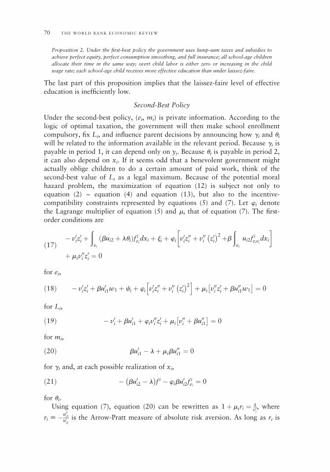
Under the second-best policy, (ei, mi) is private information. According to thelogic of optimal taxation, the government will then make school enrollmentcompulsory, fix Li, and influence parent decisions by announcing how gi and ui

will be related to the information available in the relevant period. Because gi ispayable in period 1, it can depend only on yi. Because ui is payable in period 2,it can also depend on xi. If it seems odd that a benevolent government mightactually oblige children to do a certain amount of paid work, think of thesecond-best value of Li as a legal maximum. Because of the potential moralhazard problem, the maximization of equation (12) is subject not only toequation (2) – equation (4) and equation (13), but also to the incentive-compatibility constraints represented by equations (5) and (7). Let wi denotethe Lagrange multiplier of equation (5) and mi that of equation (7). The first-order conditions are

� v0iz0i þð

xi

bui2 þ luið Þf ieidxi þ ji þ wi v0iz

00i þ v00i z0i

� �2þbð

xi

ui2f ieiei

dxi

�

þ miv00i z0i ¼ 0

ð17Þ

for ei,

� v0iz0i þ bu0i1w1 þ ci þ wi v0iz

00i þ v00i z0i

� �2h i

þ mi v00i z0i þ bu00i1w1

�¼ 0ð18Þ

for Li,

� v0i þ bu0i1 þ wiv00i z0i þ mi v00i þ bu00i1

�¼ 0ð19Þ

for mi,

bu0i1 � lþ mibu00i1 ¼ 0ð20Þ

for gi and, at each possible realization of xi,

� bu0i2 � l� �

f i � wibu0i2f iei¼ 0ð21Þ

for ui.Using equation (7), equation (20) can be rewritten as 1þ miri ¼ l

v0i, where

ri ; �u00i1

u0i1

is the Arrow-Pratt measure of absolute risk aversion. As long as ri is


nonincreasing in i’s income,21 and given that v0i is decreasing in yi,

gi ¼ g yið Þ; g0 , 0:ð22Þ

Condition (21) may be similarly rewritten as 1þ wifei

f i ¼ lbu0

i2. Because

fei

f i is

increasing in xi, and u0i2 in ui,

ui ¼ u xið Þ; u0 , 0:ð23Þ

Because there is nothing to prevent gi from falling below zero for some yi, gi

can be interpreted as the difference between an education grant equal to p22

and an earmarked tax increasing in parent income. Similarly, because there isnothing to stop ui from being negative for some xi, ui can be interpreted as thedifference between another earmarked tax, equal to p, and another educationgrant, this time increasing in the school result.

Having established that g(.) and u (.) are decreasing functions, it is clear thatthe policy redistributes from the rich to the poor and insures parents and chil-dren against the risk of a low return to effective education. Comparingequation (20) with equation (15), and equation (21) with equation (16),however, it is also clear that the policy does not go as far as the first-bestpolicy does. The reason is that redistribution has an efficiency cost, because thegovernment cannot use personalized lump-sum transfers as under the first-bestpolicy. What happens to (ei, Li, mi)? Compare equation (17) with equations (4)and (5) to see that ei is lower than under the first-best policy. In particular,because (yi þ gi) is not the same for all i, ei increases with yi, as (albeit moreslowly than) under laissez-faire. Because gi can be negative, it cannot be ruledout that ei will be lower than under laissez-faire for some i. Because the govern-ment can borrow against

Ðxiuif

idxi, however, gi will be negative only if yi isvery high. Because the government is also insuring parents against the risk of alow return to effective education, it is thus unlikely that ei will be lower thanunder laissez-faire for any i. Comparing equation (18) with equation (6) alsoshows that Li will be no higher than under either the first-best policy or laissez-faire. The intuition is that if w1 is high enough for the efficient Li to be posi-tive, imposing a ceiling on overt child labor will distort the allocation of i’stotal working time between overt and covert labor and thus make work as awhole less attractive than education. Comparing equation (19) with equation(7) shows that mi will be lower than under either the first-best policy orlaissez-faire.

Proposition 3. Under the second-best policy school enrollment is compulsory, and all school-age

children, with the possible but unlikely exception of those from very rich families, receive more

effective education than under laissez-fare; the government uses a net subsidy decreasing in

21. For evidence, see Johnson (1987).

22. Recall that subsistence consumption is normalized to zero.

Cigno 71

parent income, and a net tax decreasing in the individual skill premium, to redistribute and

insure, but stops short of perfect equity, full insurance, and perfect consumption smoothing; if

the efficient level of overt child labor is positive, the government sets a limit, lower than the effi-

cient level, on the amount of paid work a child can legally do.

The implications of relaxing some of the assumptions made so far can beintuited without formal analysis. Suppose that the returns to education invest-ment have an aggregate as well as an idiosyncratic component. Because aggre-gate risks cannot be insured against by redistributing within cohorts, thegovernment must use its ability to borrow and lend on the international creditmarket to redistribute not only within, but also between, cohorts. A similarargument applies to parent incomes. If the shocks to parent income are purelyidiosyncratic, the policy prescription remains qualitatively the same, becauseredistributing from rich parents to poor parents will insure families against therisk of a downturn in that income. The prescription also remains the samewhen the shocks have an area component, because the policy redistributes notonly within, but also between, areas. If the shocks have a countrywide com-ponent, however, the government must use its ability to borrow and lend onthe international credit market to redistribute not only within, but alsobetween, cohorts (as in the case where the aggregate shocks concern the returnto education investment).

I V. P O L I C Y P R A C T I C E I N T H E L I G H T O F T H E O R E T I C A L F I N D I N G S

Under laissez-faire, if credit and insurance markets are imperfect or contractsbetween parents and young children are unenforceable, effective education isinefficiently low. If parent income is below a certain threshold, the child willnot enroll at school. Above that threshold, the child will enroll, but childrenfrom poor families will receive less effective education than children from richfamilies. This prediction is consistent with evidence in Ram and Schultz(1979), Jacoby (1994), Jacoby and Skoufias (1997), Belzil and Hansen (2002),and Fuwa and others (2009) that inability to borrow and insure reduces edu-cation investment. It is consistent also with evidence, surveyed in Fasih (2008),that the return to measurable education inputs such as school enrollment orattendance is positive and particularly large in low- to middle-income countriesbut lower for poor children than for rich children. Because the amount of effec-tive education that children receive in a year of school enrollment or day ofschool attendance is lower if they come from a family with low parent incomethan if they come from one with high parent income, the return to enrollmentor attendance will in fact understate the return to effective education of poorchildren relative to that of rich children. This explanation does not conflictwith other possible explanations, such as that poor children have access topoor quality schools only.

The optimal (first- or second-best) policy relaxes the credit constraint oneducation investment by giving parents an advance on the expected return and


provides insurance against the risk of a low return by redistributing from luckyto unlucky school leavers. Because it redistributes from rich parents to poorparents, it will also reduce inequality and, if parent income is uncertain,provide insurance against the risk of a downturn in that income. The first-bestpolicy uses personalized lump-sum transfers to achieve perfect equity, fullinsurance, and perfect consumption smoothing. Because children are ex anteidentical, all parents enroll their children at school and give each child thesame efficient amount of effective education. The second-best policy also redis-tributes and insures. Because it cannot use personalized lump-sum transfers,however, it stops short of perfect equity, full insurance, and perfectconsumption-smoothing. It also raises effective education above the laissez-faire level for most children, but not to the efficient level. Although the worstforms of child labor are outside the scope of this analysis, a policy thatencourages effective education will discourage all forms of covert child labor,including the worst ones.

Under the second-best policy school enrollment is compulsory (whereasunder the first-best policy, it does not need to be compulsory because it is inthe interest of all parents to send their children to school). If the child wagerate is high enough for the efficient level of overt child labor to be positive, thegovernment will also impose a legal ceiling, lower than the efficient level, onsuch labor. This distorts the mix of overt and covert child labor and thusmakes child labor as a whole less attractive relative to education. Furthermore,the government makes a transfer decreasing in parent income to every schoolchild and exacts a transfer decreasing in the individual education result fromevery school leaver. The first transfer can be interpreted as the differencebetween a need-based education grant, covering maintenance and tuition, andan earmarked tax increasing in parent income. Similarly, the second transfercan be interpreted as the difference between an earmarked tax, equal to (thecapitalized value of) the need-based education grant, and a merit-based edu-cation grant increasing in the school result. The first transfer may be negativefor school-age children from families with high parent income. If the expectedreturn to effective education is high enough, however, this transfer may bepositive for anyone. The second transfer may be negative for school leaverswith a high education result. In the model the first transfer occurs at the begin-ning of the education process, and the second at the end. In practice, however,the government could deliver the need-based grant and collect the tax onparent income in installments over the education period. Similarly, it coulddeliver the merit-based grant in installments over the education period, aspartial results become available, and collect the tax on school leavers, again ininstallments, as the individual skill premia gradually unfold.

The analysis here is tailored for a poor developing country; it may be inter-esting to compare the results with those of a model tailored for a rich devel-oped economy. Hanushek, Leung, and Yilmaz (2003) use a calibrated generalequilibrium model to assess the welfare effects of a range of policy instruments,

Cigno 73

including need- and merit-based education grants, under the assumptions thatchild labor is out of the question and that parents are rich enough to be riskneutral (or, equivalently, that there is a well developed insurance market). Insuch a world, education subsidies generally perform worse than other forms ofredistribution, and a merit-based education grant can be justified only in thepresence of an education externality (while the current study finds that it isoptimal anyway). These differences highlight the importance of the stage ofdevelopment in designing education policy.

In most countries primary school enrollment is compulsory, and work at avery young age is forbidden (though enforcement is not always effective). Inpoor developing countries education is subsidized only through the price ofschool enrollment, if at all. Is that better than nothing? That question is bestanswered in two steps. First, starting from laissez-faire, would compulsoryschool enrollment raise social welfare? The answer is no, because it wouldoblige all parents, including those who would not let their children studyanyway, to bear the tuition cost. Forbidding child labor instead, or on top, ofthat would also reduce welfare, because the ban would apply only to overtchild labor, thereby distorting time allocation. Second, given compulsoryenrollment, and with or without a ban on child labor, would a price subsidyraise welfare? If the subsidy is financed by a poll tax, the policy will affectwelfare to the extent that the number of children varies across families. If allfamilies had the same number of children, the policy would have no effect,because the parents would be taking a lump-sum subsidy with one hand andgiving it back with the other. If the number varies exogenously across families,the policy will affect welfare, but the effect will be positive only if the marginalutility of income is higher in families with many children than in families withfew children (in other words, if income and fertility are not positively corre-lated). If fertility is endogenous, the policy could actually reduce welfare,because it will trigger a substitution of quantity for quality of children; seeCigno (1986). If the subsidy is financed by a tax increasing in parent income,the net transfer schedule will look almost like g(.), though not exactly the samebecause a price subsidy cannot be larger than the price, and may thus be insuf-ficient for a second-best policy. In any case, a second-best policy would alsorequire some form of insurance against the risk of a low return to effective edu-cation. In other words, the u(.) schedule is needed too.

Finally, considerable attention has been given to schemes that effectively paychildren to attend school, such as Mexico’s Programa de Educacion, Salud yAlimentacion.23 Skoufias and Parker (2001) find evidence that such schemesencourage school attendance and discourage child labor. If the nonobservabledeterminants of effective education were positively correlated with the observa-ble ones, one could be confident that offering transfers conditional on observa-ble determinants would encourage nonobservable determinants. But there is

23. For a comprehensive exposition, see Fiszbein, Schady, and Ferreira (2009).


evidence that the correlation is actually negative. Ravallion and Woodon(2000) report that the increase in school attendance elicited by an enrollmentsubsidy is four to eight times larger than the corresponding reduction in childlabor. Consistent with this finding, Fuwa and others (2009) estimate that acredit constraint reduces average school attendance by 60 percent, but raiseschild labor by double that percentage. Why? The answer given by the currentstudy’s model is that paying a child to attend school triggers a substitutionaway from not only labor but also homework and rest. This has an efficiencycost and may actually reduce effective education time. The model furthershows that paying a child to attend school will crowd out parent transfers(parents will give their children less money or take more money away fromthem).

In the light of these theoretical results and empirical findings, cash transfersshould be made conditional not only on the child attending school, but also onthe child doing no more than a certain amount of overt labor (less than the effi-cient amount, if that is positive). Furthermore, cash transfers to children in thescheme should be increasing in education results and decreasing in parentincome. Such corrections would improve the scheme but would not be enoughfor a second-best policy, because the parents would still get no insuranceagainst the risk of a low-skill premium, let alone against the risk of a negativeshock to their own income. Of course, the distance from the second best willbe even greater if parent income is private information or if overt child labor isnot overt after all, because it will then be impossible to make cash transfersconditional on either or both of these variables.

The optimal taxation approach adopted in this study gives new insights intohow best to discourage labor at a very young age and provide all children aneffective education, in poor developing countries. One such insight is that sub-sidizing school attendance without rewarding school attainment at the sametime is not optimal and may even be counterproductive. Another is that, in asecond-best perspective, it is optimal to force overt child labor below its effi-cient level, if this is positive, despite the fact that (indeed, precisely because)covert child labor cannot be similarly regulated. The analysis lends support tothe notion that school enrollment should be made compulsory but not necess-arily to the notion that overt child labor should be banned. These resultsshould help in designing a universal education system and in improving partialforms of public intervention such as conditional cash transfers.

RE F E R E N C E S

Alderman, H., P. F. Orazem, and E. M. Paterno. 2001. “School Quality, School Cost, and the Public/

Private School Choices of Low-Income Households in Pakistan.” Journal of Human Resources 36:

304–26.

Baland, J. M., and J. A. Robinson. 2000. “Is Child Labor Inefficient?” Journal of Political Economy

108: 663–79.

Cigno 75

Balestrino, A., A. Cigno, and A. Pettini. 2002. “Endogenous Fertility and the Design of Family

Taxation.” International Tax and Public Finance 9: 175–93.

Beegle, K., R. H. Dehejia, and R. Gatti. 2006. “Child Labor and Agricultural Shocks.” Journal of

Development Economics 81: 80–96.

Belzil, C., and J. Hansen (2002). “Unobserved Ability and the Return to Schooling.” Econometrica 70:

2075–91.

Besley, T. 1995. “Non-Market Institutions for Credit and Risk-Sharing in Low-Income Countries.”

Journal of Economic Perspectives 9: 115–27.

Card, D. 1999. “The Causal Effect of Education on Earnings.” In O. Ashenfelter, and D. Card, eds.,

Handbook of Labor Economics. Vol. 3. Amsterdam: North Holland.

Cigno, A. 1986. “Fertility and the Tax-Benefit System: A Reconsideration of the Theory of Family

Taxation.” Economic Journal 96: 1035–51.

———. 1993. “Intergenerational Transfers Without Altruism: Family, Market and State.” European

Journal of Political Economy 9: 505–18.

———. 2001. “Comparative Advantage, Observability, and the Optimal Tax Treatment of Families

With Children.” International Tax and Public Finance 8: 455–70.

———. 2006. “A Constitutional Theory of the Family.” Journal of Population Economics 19: 259–83.

———. 2011. “Agency in Family Policy: A Survey.” CESifo Economic Studies 57: 305–31.

Cigno, A., and A. Luporini. 2009. “Scholarships or Student Loans? Subsidizing Higher Education in the

Presence of Moral Hazard.” Journal of Public Economic Theory 11: 55–87.

Cigno, A., and F. C. Rosati. 2005. The Economics of Child Labour. New York and Oxford: Oxford

University Press.

Cremer, H., A. Dellis, and P. Pestieau. 2003. “Family Size and Optimal Income Taxation.” Journal of

Population Economics 16: 37–54.

Dessy, S. E., and S. Pallage. 2005. “A Theory of the Worst Forms of Child Labor.” Journal of

Development Economics 115: 68–87.

Dessy, S. E., and T. Rambeloma. 2010. “Is Temporary Emigration of Unskilled Workers a Solution to

the Child Labor Problem?” Cahiers de Recherche 1037. Centre Interuniversitaire sur le Risque, les

Politiques Economiques et l’Emploi, Montreal, Canada.

Epstein, G. S., and N. Kahana. 2008. “Child Labor and Temporary Emigration.” Economics Letters

99: 545–48.

Fasih, T. 2008. Linking Education Policy to Labor Market Outcomes. Washington, DC: World Bank.

Fiszbein, A., N. Schady, and F. H. G. Ferreira. 2009. Conditional Cash Transfers: Reducing Present and

Future Poverty. Washington, DC: World Bank.

Fitzsimons, E. 2007. “The Effects of Risk on Education in Indonesia.” Economic Development and

Cultural Change 56: 1–25.

Fuwa, N., S. Ito, K. Kubo, T. Kurosaki, and Y. Sawada. 2009. “How Does Credit Access Affect

Children’s Time Allocation? Evidence from Rural India.” Discussion Paper 183. Japan External

Trade Organization, Institute of Developing Economies, Chiba, Japan.

Hanson, G. H., and C. Woodruff. 2003. “Emigration and Education Attainment.” University of

California–San Diego.

Hanushek, E. A., C. K. Y. Leung, and K. Y. I. Yilmaz. 2003. “Redistribution through Education and

Other Transfer Mechanisms.” Journal of Monetary Economics 50: 1719–50.

Jacoby, H. 1994. “Borrowing Constraints and Progress Through School: Evidence from Peru.” Review

of Economics and Statistics LXXVI: 151–60.

Jacoby, H., and E. Skoufias. 1997. “Risk, Financial Markets and Human Capital in Developing

Countries.” Review of Economic Studies 64: 311–35.

Johnson, W. R. 1987. “Income Redistribution as Human Capital Insurance.” Journal of Human

Resources 22: 269–80.


Kahneman, D. 2003. “Maps of Bounded Rationality: Psychology for Behavioral Economics.” American

Economic Review 93: 1449–75.

Kanbur, R., J. Pirttila, and M. Tuomala. 2008. “Moral Hazard, Income Taxation and Prospect

Theory.” Scandinavian Journal of Economics 110: 321–37.

Kodde, A. D. 1986. “Uncertainty and the Demand for Education.” Review of Economics and Statistics

68: 460–67.

Levhari, D., and Y. Weiss. 1974. “The Effect of Risk on the Investment in Human Capital.” American

Economic Review 64: 950–63.

Loury, G. 1981. “Intergenerational Transfers and the Distribution of Earnings.” Econometrica 49:

843–67.

Oreopoulos, P. 2006. “Average Treatment Effects of Education when Compulsory School Laws Really

Matter.” American Economic Review 96: 152–75.

Pouliot, W. 2006. “Introducing Uncertainty in Baland and Robinson’s Model of Child Labour.”

Journal of Development Economics 79: 264–72.

Ram, R., and T. Schultz. 1979. “Life Span, Health, Savings and Productivity.” Economic Development

and Cultural Change 13: 399–421.

Ranjan, P. 2001. “Credit Constraints and the Phenomenon of Child Labor.” Journal of Development

Economics 64: 81–102.

Ravallion, M., and Q. Woodon. 2000. “Does Child Labour Displace Schooling? Evidence on

Behavioural Responses to an Enrolment Subsidy.” Economic Journal 110: c158–c175.

Razin, A. 1976. “Lifetime Uncertainty, Human Capital and Physical Capital.” Economic Enquiry 14:

439–48.

Skoufias, E., and S. Parker. 2001. “Conditional Cash Transfers and the Impact on Child Work and

Schooling. Evidence from Mexico’s Progresa Program.” Economia 2: 45–96.

Townsend, R. 1994. “Risk and Insurance in Village India.” Econometrica 62: 539–92.

Cigno 77

how to deal with covert child labor and give children an...

Documents