how to design target-date funds? - thierry roncallithierry-roncalli.com/download/lwp-tdf.pdf · how...

How to Design Target-Date Funds?∗

Benjamin BruderResearch & Development

Lyxor Asset Management, [email protected]

Léo CulerierResearch & Development


Thierry RoncalliResearch & Development


September 2012

AbstractSeveral years ago, the concept of target-date funds emerged to complement tra-

ditional balanced funds in defined-contribution pension plans. The main idea is todelegate the dynamic allocation with respect to the retirement date of individuals tothe portfolio manager. Owing to its long-term horizon, a target-date fund is uniqueand cannot be compared to a mutual fund. Moreover, the objective of the individualis to contribute throughout their working life by investing a part of their income inorder to maximise their pension benefits. The main purpose of this article is to analyseand understand dynamic allocation in a target-date fund framework. We show thatthe optimal exposure in the risky portfolio varies over time and is very sensitive tothe parameters of both the market and the investor’s. We then deduce some practicalguidelines to better design target-date funds for the asset management industry.

Keywords: target-date fund, retirement system, dynamic asset allocation, stochastic opti-mal control, market portfolio, risk aversion, stock/bond asset mix policy.

JEL classification: C61, D91, G11, J26.

1 IntroductionIn 1952, Markowitz introduced the first mathematical formulation for portfolio optimisa-tion. For Markowitz, “the investor does (or should) consider expected return a desirablething and variance of return an undesirable thing”. Indeed, Markowitz shows that an effi-cient portfolio is the portfolio that maximises the expected return for a given level of risk(corresponding to the variance of return). Markowitz concludes that there is not only oneoptimal portfolio, but a set of optimal portfolios which is called the ‘efficient frontier’. Bystudying the liquidity preference, Tobin (1958) shows that the efficient frontier becomes astraight line in the presence of a risk-free asset. In this case, optimal portfolios correspondto a combination of the risk-free asset and one particular efficient portfolio named the tan-gency portfolio. Sharpe (1964) summarises Markowitz and Tobin’s results as follows: “the

∗We are grateful to Karl Eychenne and Nicolas Gaussel for their helpful comments.

How to Design Target-Date Funds?

process of investment choice can be broken down into two phases: first, the choice of aunique optimum combination of risky assets1; and second, a separate choice concerning theallocation of funds between such a combination and a single riskless asset”. This two-stepprocedure is today known as the separation theorem (Lintner, 1965).

In Figure 1, we have illustrated these results. The first panel represents the efficient fron-tier of Markowitz between equities and bonds. By combining the mean-variance optimisedportfolio with the higher Sharpe ratio and the risk-free rate, we obtain the capital marketline. In the second panel, we have reported the risk/return profile of optimal portfolios cor-responding to different values for the risk aversion parameter. The aggressive (A) investorleverages the tangency portfolio in order to take more risk and to expect better performance.For the moderate (M) investor, the optimal portfolio is closed to the tangency portfolio. Theconservative (C) investor will take less risk, hence the reason why they allocate their wealthbetween the tangency portfolio (risky assets) and the risk-free asset. This theoretical viewof asset allocation is however far from the ‘popular advice’ on portfolio allocation. In thethird panel, we have shown typical diversified funds designed by the asset management in-dustry. Generally, we distinguish three fund profiles: defensive, balanced and dynamic. Thedifference between them comes from the relative proportion of stocks and bonds2. It meansthat in practice, the composition of the risky portfolio varies according to the investor’s riskaversion. This portfolio construction contradicts the separation theorem, which states thatthe composition of the risky portfolio should be the same for all investors. This paradox,known as the asset allocation puzzle (Canner et al., 1997), has resulted in wealth of literaturebeing written in an attempt to find some explanations (see Campbell (2000) for a survey).

Figure 1: The asset allocation puzzle

1It is precisely the tangency portfolio.2For a defensive fund, the proportion of stocks and bonds is 20% and 80% respectively, whereas they are

the reverse for the dynamic fund. In the case of the balanced fund, we have the same proportions.

2


Another puzzle concerns lifecycle funds or target-date funds. In a lifestyle fund likediversified funds, the asset mix policy depends on the risk aversion (or the lifestyle) of theinvestor. In a target-date fund, the asset mix policy depends on the time to retirement ofthe investor. In Figure 2, we have reported the dynamic asset allocation of a typical target-date fund3. When the individual is young, they invest principally in equities whereas theallocation will be more heavily weighted toward bonds (or cash) as they approach retirement.The speed with which a target-date fund changes its asset allocation is known as the ‘glidepath’.

Figure 2: An example of glide path

These funds have been gaining popularity since early 21st century. One of the reasons isthe major shift from defined benefit (DB) toward defined contribution (DC) pension plansand the transfer of investment risk from the corporate sector to households. Another reasonconcerns certain regulatory reform and tax benefits. For example, the Pension ProtectionAct of 2006 in the US requires companies who have underfunded their pension plans to payhigher premiums to the Pension Benefit Guaranty Corporation. DB liabilities may inducelarge pension costs for the sponsor and incite it to promote DC pension plans. In thiscontext, it is not surprising that target-date funds encounter high growth:

“Target-date funds are fast becoming a fixed feature of the defined-contributionlandscape. Over the past half dozen years, assets in target-date funds havegrown more than fivefold from $71 billion at the end of 2005 to approximately$378 billion at year-end 2011. In its most recent study, Vanguard reported that82% of its retirement plans offered target-date funds, and nearly one fourth ofparticipants invested only in a target-date fund. The consultant Casey Quirkestimates that target-date funds will consume more than half of all defined-contribution assets by 2020” (Morningstar [39], 2012).

3τ = T − t is the remaining time until the retirement.

3


It is also a concentrated industry, because, according to the Morningstar report, three assetmanagers (Fidelity, Vanguard and T. Rowe Price) hold 78% of the target-date mutual funds.The previous figures only concern open target-date assets and not the overall target-dateassets managed in retirement systems. The Investment Company Institute (2012) reportsthat U.S. retirement assets were $17.9 trillion at year-end 2011. The largest components areIRAs ($4.9), DC plans ($4.5) and private-sector DB pension funds ($2.4). For DC plans,the asset allocation depends on the age of participants:

“On average, younger participants allocate a larger portion of their portfolio toequities [...] According to research conducted by ICI and the Employee Ben-efit Research Institute (EBRI), at year-end 2010, individuals in their twentiesinvested 44% of their assets in equity funds and company stock, 37% in target-date funds and non-target-date balanced funds [...] All told, participants intheir twenties had 74 percent of their 401(k) assets in equities. By comparison,at year-end 2010, individuals in their sixties invested 41% of their assets in eq-uity funds and company stock, 16% in target-date funds and non-target-datebalanced funds [...] All told, participants in their sixties had 49% of their 401(k)assets in equities” (Investment Company Institute [27], 2012).

Indeed, target-date funds represent 27% and 9% respectively of the DC plan assets forindividuals in their twenties and in their sixties. This therefore confirms the appeal oftarget-date funds for younger participants.

Figure 3: Allocation of the Fidelity ClearPath R⃝ 2045 Retirement Portfolio

Source: www.fidelity.ca/cs/Satellite/en/public/products/managed_solutions/clearpath.

One of the big challenges of target-date funds is the design of glide paths. Let usconsider for example the Fidelity ClearPath R⃝ Retirement Portfolios. In Figure 3, we havereported the dynamic allocation for Canadian individuals who will retire in 40 years using

4


the simulation tool provided on Fidelity’s web site. We notice how the split between stocks,bonds and cash evolves in relation to time. The allocation becomes more conservative whenwe approach the retirement date: equities represent more than 80% of the portfolio todaywhereas their weight is only 31% in 50 years’ time; the bond allocation increases during25 years and then stabilises at around 30%; the weight of the high yield asset class variesbetween 7% and 5% and therefore is very stable; the allocation in cash begins 12 yearsbefore the retirement date and represents 35% at the end. If we consider other target-datefunds, glide paths present similar patterns on average. But differences among target-datefunds may be very large. For example, Morningstar (2012) reports that equity allocationvaries between 20% (38% and 85% respectively) and 78% (86% and 100% respectively) ifthe target year is 2015 (2025 and 2055 respectively). It is rather surprising to obtain suchbroad allocation range particularly for shorter target dates.

There are many popular justifications given for these allocations (Quinn, 1991), but mostof them does not make economic sense (Jagannathan and Kocherlakota, 1996). Hence thereason why academic research may help to understand this asset allocation puzzle. Theseminal work of Merton (1969, 1971) is the usual framework used to analyse dynamic assetallocation. Most research introduces some clarifications of the Merton model. For example,Munk et al. (2004) consider the mean-reverting property of equity returns and the uncer-tainty of inflation risk. By calibrating their model with historical US data from the period1951-2003, they found results consistent with the investment recommendation “more stocksfor longer-term investors”. This research confirms the conclusion made by Brennan and Xia(2002) that the optimal stock-bond mix depends on the investor’s horizon in the presence ofinflation risk and highlights the influence of mean reversion4. Other clarifications concernthe behaviour of optimal allocation in the latter years before the retirement date (Basu andDrew, 2009), the effect of the stock-bond correlation on hedging demand (Henderson, 2005),the labour supply flexibility (Bodie et al., 1992), the longevity risk (Cocco and Gomez, 2012),the effect of real estate assets (Martellini and Milhau, 2010) and the return predictability(Larsen and Munk, 2012).

Although the various clarifications are interesting to understand the allocation of target-date funds, they are not enough to explain the dynamics of glide paths. Labour incomeis generally the key factor to understanding their behaviour. It explains the breadth ofliterature on the relationship between stock-bond asset mix and labour income5. Our paperadopts this approach by considering stochastic permanent contribution to the target-datefund. In this case, we show that the behaviour of optimal exposure is similar to many glidepaths used in the investment industry. Nevertheless, we also notice that the solution is verysensitive to input parameters like the equity risk premium, the contribution uncertainty orthe stock-bond correlation. But the most important factor concerns the personal profile ofthe individual. The degree of risk aversion, retirement date and income perspective of theinvestor are certainly the key elements to design target-date funds.

Our paper is organised as follows. Section two presents the theoretical model based onthe Merton framework. Since we assume that interest rates and permanent contribution arestochastic, we have to solve the optimisation problem by considering numerical analysis. InSection three, we analyse the dynamics of risky exposure and define the glide path. Then,we highlight some patterns for the design of target-date funds with respect to our theoreticalmodel. Section five offers some concluding remarks.

4See also Barberis (2000), Campbell et al. (2001) or Wachter (2002) for related results.5We could cite for example the works of Bodie et al. (2004), Cocco et al. (2005), Gomes and Michaelides

(2005), Henderson (2005), Munk and Sørensen (2010) or Viceira (2001).

5


2 A theoretical modelWe consider the intertemporal model of Merton (1971) in which we introduce a stochasticpermanent contribution πt. It is the main difference between the design of a mutual fundand a target-date fund:

• In a mutual fund, the individual makes an initial investment and seeks to maximisethe net asset value for a given horizon. Generally, the investment horizon for suchfunds is three or five years;

• In a target-date fund, the individual makes an initial investment and continues tocontribute throughout their working life. The investor’s objective is then to maximisetheir pension benefits during retirement.

Another difference between a mutual fund and a target-date fund concerns then the invest-ment horizon. The latter is typically equal to forty years.

Generally, retirement system models do not use permanent contribution πt as a statevariable, but prefer to consider labour income Lt. Of course, most of the permanent contri-bution comes from a savings component related to labour income and we can link these twostate variables as follows:

πt = ϖtLt

where ϖt is the savings ratio of the individual. But this equation ignores the possibilitythat the permanent contribution could come from family heritage, from inheritance or evenfrom the employer’s funding contribution system6. Hence why we prefer to consider thepermanent contribution, and not the labour income, as a (exogenous) state variable.

2.1 The frameworkLet us first introduce some notations. We consider a target-date fund with maturity Towned by only one investor. Its value at time t is denoted by Xt. It could be invested in arisky portfolio St with a proportion αt and in a zero-coupon bond Bt,T with a proportion1 − αt. Since the investor has some income or private wealth and would like to use thetarget-date fund for retirement pension benefits, they regularly contribute to the fund. Wenote their contribution as πt. The dynamics of the target-date fund is then:

dXt

Xt= αt

dSt

St+ (1− αt)

dBt,T

Bt,T+

πt dt

Xt

Let us now precise the dynamics of St, Bt,T and πt. For this last one, we assume thatπt = ptQt where pt is the average contribution behaviour for the representative agent andQt is a random factor related to contribution uncertainty. The state variable Qt is important,because the investor does not know exactly what their contribution will be in the future.We then have:

dSt = µtSt dt+ σtSt dWSt

dQt = θtQt dt+ ζtQt dWQt

dBt,T = rtBt,T dt+ Γt,TBt,T dWBt

6This last case may be illustrated by the French PERCO retirement system. The individual contributionis completed by a (capped) employer contribution πE

t . It implies that the permanent contribution becomes:

πt = ϖtLt + πEt

The objective of individuals is generally to obtain the maximum contribution πEmax of the employer meaning

that the permanent contribution is not a proportion of the labour income.

6


Let Wt =(WS

t ,WQt ,WB

t

)be the vector of brownian motions. We assume that:

E[WtW

⊤t

]=

1 ρS,Q ρS,BρS,Q 1 ρQ,B

ρS,B ρQ,B 1

dt

2.2 Optimal solutionLet U (x) be the investor’s utility function which depends on the value x reached by thefund. We assume that their objective is to maximise their utility at time T . We then have:

α∗t = argmaxEt [U (XT )]

The investor’s problem is then to find the optimal level of exposure α∗t to the risky portfolio

depending on the behaviour of the assets and the investor’s contribution policy. Since wecannot obtain a closed formula for α∗

t , we use stochastic optimal control.

We use the zero-coupon bond Bt,T of maturity T as the numéraire. We introduce thenotation Xt,T = Xt/Bt,T . As the self-financing condition is invariant by change of numéraire(El Karoui et al., 1995), we obtain:

dXt,T

Xt,T= αt

dSt,T

St,T+

πt dt

Bt,TXt,T

In Appendix A.1, we show that the forward dynamics of (Xt, Qt) is:{dXt,T = (αtµt,TXt,T + ptQt,T ) dt+ αtσt,TXt,T dBS

t

dQt,T = θt,TQt,T dt+ ζt,TQt,T dBQt

with7: µt,T = µt − rt + Γ2

t,T − ρS,BσtΓt,T

σt,T =√σ2t + Γ2

t,T − 2ρS,BσtΓt,T

θt,T = θt − rt + Γ2t,T − ρQ,BζtΓt,T

ζt,T =√ζ2t + Γ2

t,T − 2ρQ,BζtΓt,T

BSt and BQ

t are two brownian motions such that E[BS

t BQt

]= ρ⋆ dt with:

ρ⋆ =ρS,Qσtζt − ρS,BσtΓt,T − ρQ,BζtΓt,T + Γ2

t,T

σt,T ζt,T(1)

Let J be the function defined by:

J (t, x, q) = supα

Et [U (XT ) | Qt,T = q,Xt,T = x]

The optimal exposure is then given by this relationship8:

α∗t = −

µt,T∂xJ (t, x, q) + ρ⋆σt,T ζt,T q∂2x,qJ (t, x, q)

xσ2t,T∂

2xJ (t, x, q)

(2)

7To obtain this result and to solve our model, we have to introduce some technical restrictions to theprocess µt − rt and θt − rt so that Xt,T and Qt,T are two Markov processes. For example, our analysis isvalid if µt − rt and θt − rt are deterministic.

8See Appendix A.2 for more details.

7


2.3 Some specific casesLet us first consider that the investor does not contribute to the fund. In this case, πt = 0and the solution (2) reduces to:

α∗t = − µt,T∂xJ (t, x)

xσ2t,T∂

2xJ (t, x)

(3)

Moreover, if we assume that the interest rate is constant and the parameters µt and σt donot depend on time t, we obtain Merton’s well-known result (1969):

α∗t = − (µ− r)

σ2· ∂xJ (t, x)

x∂2xJ (t, x)

In the case of the CRRA utility function U (x) = xγ/γ with γ < 1, the proportion of therisky portfolio remains constant for the entire period [0, T ] and does not depend on the valuex of the fund:

α∗t =

(µ− r)

(1− γ)σ2= α (4)

The constant mix strategy is then the optimal dynamic allocation strategy.

If Qt = 1, it means that there is no uncertainty on the future contribution of the investor.Moreover, if we assume that the interest rate is nul, Merton’s results (4) become:

α∗t = α+

µ∫ T

tπu du

(1− γ)σ2x(5)

Therefore, the optimal exposure depends on the future contributions to be made by theinvestor. This result was already found by Merton (1971) when he introduced noncapitalgain income:

“ [...] one finds that, in computing the optimal decision rules, the individualcapitalizes the lifetime flow of wage income as the market (risk-free) rate ofinterest and then treats the capitalized value of an addition to the current stockof wealth ” (Merton (1971), page 395).

3 Dynamics of the risky exposureIn this section, we study the dynamics of the risky exposure α∗

t with respect to the differentparameters. First, we analyse the impact of permanent contribution. Second, we defineprecisely what the glide path of a target-date fund is and how it is related to the opti-mal allocation. Then, we measure the impact of the different input parameters (stochasticcontribution, stochastic interest rates and correlations) on the solution.

3.1 Comparison with the optimal solution of MertonLet us consider the equation (5). We notice that α∗

t is an increasing function of the expectedreturn µ and the risk aversion parameter γ and a decreasing function of the volatility σ.We retrieve Merton’s stylised fact. We also notice that α∗

t is larger than α if πt ≥ 0. Itmeans that the investor is more exposed in a target-date fund than in the constant mixstrategy, because of the contribution effect. The difference between α∗

t and α depends onthe behaviour of the contribution function πt and the value of the wealth x of the investor.

8


It is an increasing function of the ratio between the future contributions and the actual valueof the target-date fund. In Table 1, we have shown the numerical values taken by α∗

t whenµ = 3%, σ = 15%, γ = −3 and πt = π. In this case, the optimal exposure of the constantmix strategy is 33.3%. If we suppose that the investor plans to have a future cumulativecontribution Πt =

∫ T

tπu du equal to their actual wealth, the optimal exposure is then twice

the exposure α obtained by Merton9. If the future contribution is relatively small comparedto the actual wealth, the exposure is close to the exposure of the constant mix strategy. Wecould then deduce the following economic behaviour of the investor:

• the exposure is an increasing function of the maturity because the future contributionΠt is an increasing function of the remaining time T − t; It implies, for example, thata young worker has greater exposure than an individual close to retirement;

• the exposure is smaller for an investor who does not expect to have significant futureincome with respect to their initial wealth than for an investor for whom future growthis expected to be significant; this implies that individuals take less risk if they havemore initial wealth.

These different properties are illustrated in Figure 4 with the previous values of the param-eters µ, σ and γ. We assume that πt = 5% while T is fixed to 40 years. In the first panel,we confirm that exposure decreases with the value of the wealth x and the time10 t. In thetop-right panel, we illustrate the impact of the wealth x. The smaller the wealth, the greaterthe risk exposure.

Table 1: Optimal exposure α∗t (in %) with respect to x and π

T − t = 1 year T − t = 10 yearsx/π 0 100 1000 10000 0 100 1000 100001000 33.3 36.7 66.7 366.7 33.3 66.7 366.7 3366.72000 33.3 35.0 50.0 200.0 33.3 50.0 200.0 1700.05000 33.3 34.0 40.0 100.0 33.3 40.0 100.0 700.010000 33.3 33.7 36.7 66.7 33.3 36.7 66.7 366.7100000 33.3 33.4 33.7 36.7 33.3 33.7 36.7 66.7

The initial wealth x is reported in rows whereas the future contribution π correspondsto columns. Their values are in dollars. For example, if the initial wealth is 10000

dollars and the future contribution is 1000 dollars per year, the optimal exposure α∗t

is 36.7% (respectively 66.7%) if the time to retirement T − t is 1 year (respectively10 years).

Remark 1 We notice that if we multiply the initial wealth x and the future contributionπt by the same factor, the optimal exposure does not change. We could then normalize theresults, because they only depend on the relative ratio between the future contribution andthe current wealth. For example, we verify in Table 1 that the optimal exposure for x = 1000dollars and π = 100 dollars is the same for x = 10000 dollars and π = 1000 dollars. Thisis why we normalize x and set it to 1.

9It is the case when the actual wealth x is equal to 10000 dollars, the future contribution π is 1000 peryear and the time to retirement T − t is 10 years.

10meaning that it increases with the remaining time T − t.

9


Figure 4: Computation of the risky exposure α∗t

3.2 Defining the glide pathThe glide path of the target-date fund is generally defined as dynamic asset allocation{α∗

t , t ≤ T}. In Figure 4, the bottom-left panel corresponds to two simulations of the wealthx whereas the bottom-right panel indicates the corresponding optimal exposure α∗

t . Wefirst notice that the allocation depends on the path of the wealth. It implies that optimalexposure and wealth are both endogenous:

Xt −→ α∗t −→ dXt −→ Xt+dt

Therefore, there is not one dynamic asset allocation path as illustrated in bottom-left panel.Hence why it is more pertinent to define the glide path as the expected dynamic assetallocation:

gt = E0 [α∗t ] = E [α∗

t | X0 = x0]

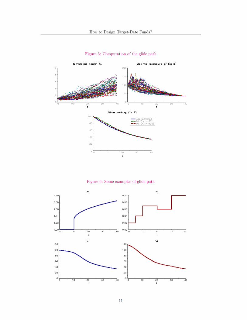
The glide path can be calculated using Monte Carlo simulations. In the case where theinterest rate is nul and the contribution function is linear, we obtain the approximatedformula given in Appendix A.4. In Figure 5, we have reported the glide path computed byMonte Carlo and by approximation11. We notice that the approximated formula gives agood result12.

The glide path depends on the shape of the contribution function πt. We give two exam-ples in Figure 6. In the first example (top-left panel), the investor does not contribute whenthey are relatively young, whereas upon retirement their contribution is at its maximum. Inthis case, we obtain the glide path given in the bottom-left panel. During 10 years, the glide

11We use the same parameters values as before. For the contribution function, a and b are set to 0.002and 0.01.

12The small difference comes from the convexity bias due to Jensen’s inequality.

10


Figure 5: Computation of the glide path

Figure 6: Some examples of glide path

11


path is approximatively constant because their future contribution remains constant. Wecould also consider an example where the contribution function is not a monotone function(top-right panel). In this case, the shape of the glide path is more complex as illustrated inthe bottom-right panel. We notice in this example that the exposure of the investor to therisky asset is leveraged at the beginning of their working life.

3.3 Introducing uncertainty on the contribution functionIn the sequel, we assume that µt = 3%, σt = 15%, θt = 0, ζt = 3%, rt = 1% and Γt,T = 0.Moreover, all the correlations are set to zero. For the utility function, we continue touse the CRRA function with γ = −3. The contribution πt is calibrated using the Frenchsaving report done by INSEE (ref. [26], Figure 6, page 114). We obtain the functionpt reported in the first panel in Figure 7. In order to better understand these data, wehave indicated the corresponding monthly contribution in the second panel. The averagemonthly contribution is equal to 1650 dollars whereas the minimum and the maximum arerespectively 880 and 1900 dollars. In the third panel, we have represented the probabilitydensity function of Qt. We verify that the variance of Qt increases with the time t due tothe economic uncertainty. Finally, the fourth panel corresponds to the quantile distributionof the cumulative contribution

∫ t

0πu du.

Figure 7: Dynamics of the contribution function πt

The representation of the optimal exposure α∗t is complicated because it depends on

three state variables: the time t, the wealth Xt and the degree of economic uncertainty Qt.Hence why we prefer to compute the glide path gt:

gt = E0 [α∗t ] = E [α∗

t | X0 = x0, Q0 = q0]

For the illustration, x0 is set to USD 10 000 and q0 is equal to 1. We have reported the glidepath gt in Figure 8. If we consider the first panel, we retrieve the typical behaviour of glide

12


paths used in the investment industry. But this glide path is valid for an investor with aninitial wealth of USD 10 000 and an average total contribution of USD 800 000 (see Figure7). If the initial wealth is equal to USD 500 000, the glide path is completely different.So, the glide paths used in the investment industry correspond to investors whose initialwealth is very small compared with their future revenues. In the second panel, we show theinfluence of economic uncertainty of future contributions. We notice that the influence ofQt is similar to the ratio between the actual wealth and the future contributions. Of course,the level of the glide path is highly dependent of the risk premium µ− r and the volatilityσ of the risky asset (Panels 3 and 4 in Figure 8). More precisely, we observe that the mostimportant factor is the Sharpe ratio divided by the volatility. This result has been alreadyexhibited by Merton (1969).

Figure 8: Glide path with random economic factor

The first panel corresponds to the glide path using default values for parameters.The second panel represents the influence of Qt which is the state variable of thecontribution uncertainty. In average, Qt is equal to 1. If Qt < 1, the realized futurecontribution is then below the expected future contribution. The third panel showsthe impact of the expected return µ of the risky asset whereas the fourth panelindicates how the glide path changes with the volatility of the risky asset.

Remark 2 More surprising is the influence of the volatility ζt, which measures the standarddeviation of the future contribution. As expected, it reduces the risky exposure, but theimpact is small (see Figure 9). One explanation is the leptokurtic behavior of the log-normaldistribution of Qt. Increasing ζt implies a more dispersed probability distribution, but withoccurrences of high values of Qt. This second effect partially compensates the effect ofdispersion. Nevertheless, the impact of ζt implies that stable future contribution induces morerisky exposures than random future contributions (the typical example concerns individualsworking in the public sector compared to individuals working in the private sector).

13


Figure 9: Influence of the volatility ζt on the glide path

3.4 Implications of stochastic interest ratesIn the previous paragraph, we assumed that the volatility Γt,T of the zero-coupon bond isequal to zero. We now consider that interest rates are stochastic. For that, we use the Hoand Lee (1995) specification:

Γt,T = φ · (T − t)

When φ = 0.1%, we obtain the results of the first panel in Figure 10. Introducing thevolatility of interest rates reduces the optimal exposure, particularly at the beginning of thetime period. To understand this result, we notice that the interest rates volatility Γt,T hasthree effects:

1. it increases the forward volatility σt,T of the risky asset St;

2. it increases the forward volatility ζt,T of the economic factor Qt;

3. it introduces a positive forward correlation ρ∗ between the risky asset and the economicfactor.

All these three effects have a negative impact on the optimal exposure α⋆t . From an economic

point of view, we could interpret this effect because the zero-coupon bond is the only asset tohedge the liabilities (which corresponds to the terminal wealth) in our model. The hedgingexposure increases then with interest rate volatilities. Hence why this effect is likely todisappear if we introduce the cash or short-term bonds in the asset universe.

3.5 What is the impact of the correlations?We continue our example by studying the influence of the correlations. The parameter φ ofthe interest rates volatility is always set to 0.1%. In Figure 10, we observe that a positive

14


Figure 10: Impact of stochastic interest rates and correlations

In the first panel, we compare the glide path with and without interest rates volatilityφ. The impact of the correlation ρS,Q between the risky asset returns and thecontribution πt is represented in the second panel. The third panel illustrates theimpact of the stock-bond correlation ρS,B .

correlation between St and Qt or a negative correlation between St and Bt,T decreases theoptimal exposure.

The parameter ρS,Q measures the correlation between the return of the risky asset andthe contribution to the fund. It is generally admitted that when the equity market performswell, the contribution is improved because the investor is encouraged to participate in thegrowth of the equity market. Another reason is that the economy is more likely to be ina period of expansion because of the positive correlation between equity performance andthe business cycle. In the Lucas (1978) model, the payoff of the risky asset has a positivecovariance with consumption, which implies that the correlation with savings is negative.For these reasons, we could admit than when St increases, Qt also increases. This explainswhy we assume that the correlation ρS,Q is positive.

For the correlation ρS,B between the risky asset and the zero-coupon bond, it is morecomplicated. Empirical works show that the stock-bond correlation is time-varying. In thelong-run, this correlation is generally positive because of the present value model. However,it is negative in periods of flight-to-quality (Ilmanen, 2003) or periods of low inflation (Ey-chenne et al., 2011). This has been the case for the past 15 years and is the reason why weprefer to impose negative correlation ρS,B .

Indeed, the impact of the correlations ρS,Q and ρS,B is more complex than presentedhere because Equation (1) shows that the results depend on the volatility of Qt, Bt,T and

15


St. Appendix A.5 presents an in-depth analysis. For the single effects, we could summarisethe results as follows:

Parameter ρS,Q ρS,B ρQ,B Γt,T σt (Γt,T ≃ 0) ζtImpact + − − ? sign of ρS,Q ?

For the multi-effects, it depends on the numerical values of the parameters.

Remark 3 ρS,Q measures the correlation between the risky asset and the permanent con-tribution. If ρS,Q is close to one, the exposure to the risky asset tends to 0. In this case,it is preferable that the individual invest a large part of their savings component into bonds.This is the typical case for employee savings plan. By investing a large part of their moneyinto the stocks of their company, individuals face the simultaneous risk of losing their joband experiencing large losses for their financial assets. But when financial income is highlycorrelated with labour income (or the economic cycle), individuals demand a high risk pre-mium. It is one of the lessons of the Lucas model and is certainly more rational to diversifyfinancial income and labour income. This explains why the exposure to the risky asset fallsto zero when the correlation tends to one.

4 Patterns of target-date fundsIn this section, we exhibit the four patterns that characterise a target-date fund. First, itis very sensitive to the personal profile of the investor. Second, a target-date fund exhibitsa contrarian allocation strategy. Third, the risk budget must be controlled. And finally,tactical asset allocation has to be considered. These four patterns help us to better designtarget-date funds as shown in the last paragraph of this section.

4.1 The personal profile of the investorWe may divide the parameters of our model into two families:

• some parameters concern the financial assets;

• other parameters relate to the individual.

These two types of parameters influence the design of the target-date fund in a different way.For example, asset parameters, like the expected return or the volatility of the risky asset,are defined by the portfolio manager. Indeed, the fund manager has the mandate to changethe allocation according to their short-term or long-term views on the different asset classes.In some sense, these parameters are endogenous and change from one portfolio manager toanother. The investors’ parameters are more exogenous and concern:

1. the retirement date of the investor;

2. the risk aversion of the investor;

3. the actual and future wealth of the investor.

These three parameters are very important for designing the target-date fund.

Most of the time in the industry, target-date funds are only structured according to retire-ment date. For example, Fidelity manages nine target-date funds called Fidelity ClearPath R⃝

Retirement Portfolios, each of them corresponding to a specific retirement date13. Thereby,13The retirement dates begin in 2005 and end in 2045 on a constant scale of 5 years.

16


the Fidelity ClearPath R⃝ Retirement Portfolio 2045 is designed for investors who will retirein or around the year 2045.

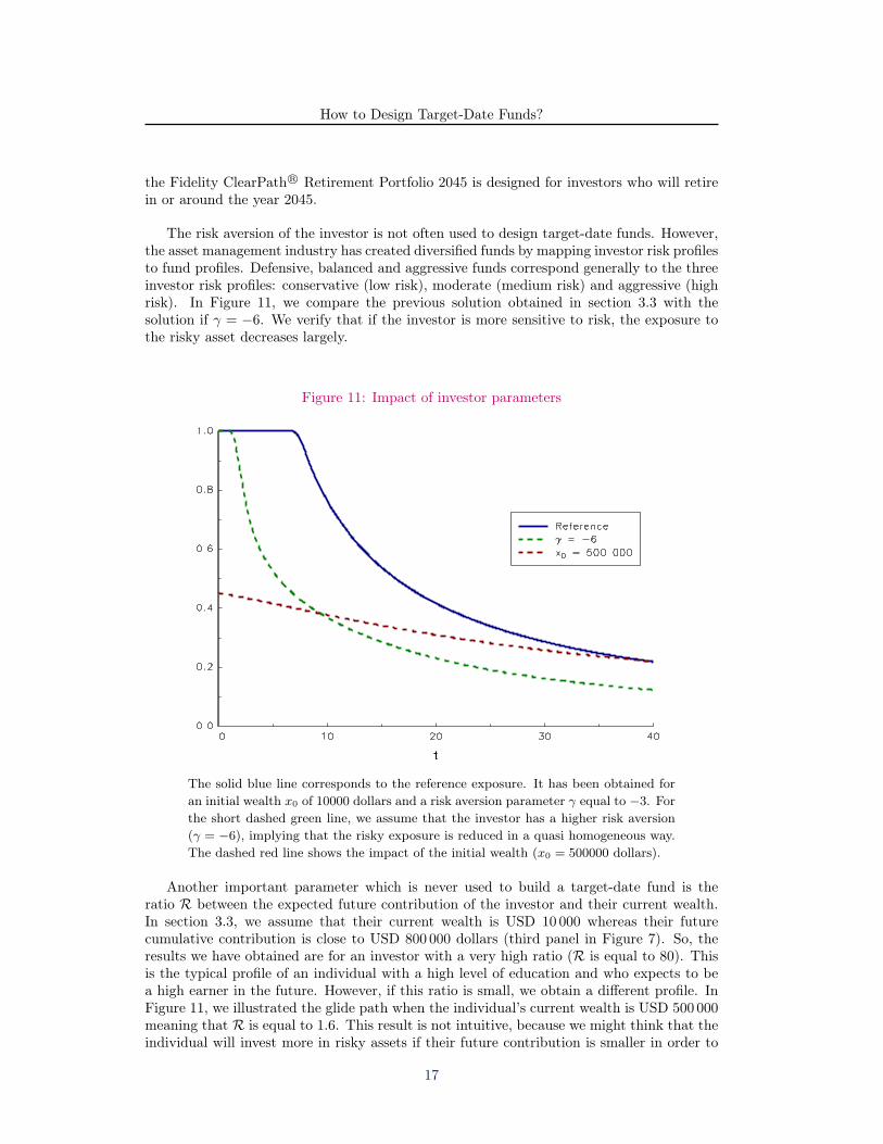
The risk aversion of the investor is not often used to design target-date funds. However,the asset management industry has created diversified funds by mapping investor risk profilesto fund profiles. Defensive, balanced and aggressive funds correspond generally to the threeinvestor risk profiles: conservative (low risk), moderate (medium risk) and aggressive (highrisk). In Figure 11, we compare the previous solution obtained in section 3.3 with thesolution if γ = −6. We verify that if the investor is more sensitive to risk, the exposure tothe risky asset decreases largely.

Figure 11: Impact of investor parameters

The solid blue line corresponds to the reference exposure. It has been obtained foran initial wealth x0 of 10000 dollars and a risk aversion parameter γ equal to −3. Forthe short dashed green line, we assume that the investor has a higher risk aversion(γ = −6), implying that the risky exposure is reduced in a quasi homogeneous way.The dashed red line shows the impact of the initial wealth (x0 = 500000 dollars).

Another important parameter which is never used to build a target-date fund is theratio R between the expected future contribution of the investor and their current wealth.In section 3.3, we assume that their current wealth is USD 10 000 whereas their futurecumulative contribution is close to USD 800 000 dollars (third panel in Figure 7). So, theresults we have obtained are for an investor with a very high ratio (R is equal to 80). Thisis the typical profile of an individual with a high level of education and who expects to bea high earner in the future. However, if this ratio is small, we obtain a different profile. InFigure 11, we illustrated the glide path when the individual’s current wealth is USD 500 000meaning that R is equal to 1.6. This result is not intuitive, because we might think that theindividual will invest more in risky assets if their future contribution is smaller in order to

17


maintain their pension benefits. But this argument means that the individual has a lowerlevel of risk aversion.

Remark 4 The previous figures of the initial wealth and the future contribution may appearto be high. Nevertheless, the glide path remains the same if we divide these two quantitiesby the same factor. For example, if x0 is equal to USD 1 000 and the future contribution isUSD 80 000, the solution always corresponds to the same reference curve.

4.2 The contrarian nature of target-date fundsLet us consider the optimal exposure α∗

t (x) at time t. If we consider the deterministic case,we obtain:

∂ α∗t (x)

∂ x≤ 0 (6)

This result remains valid if we assume that14 ∂xJ (t, x, q) ≥ 0, ∂2xJ (t, x, q) ≤ 0 and ρ⋆ = 0.

It means that the investment strategy is contrarian.

By defining the dynamic asset allocation by the glide path, the effect of the wealthdynamics vanishes. In particular, if the risky asset has performed very well during a period,the wealth of the investor increases and is certainly larger than the wealth expected:

Xt ≥ E [Xt] ⇒ α∗t ≤ gt

In this case, the target-date fund takes more risk if the dynamic asset allocation is given bythe glide path gt. We have illustrated this difference of behaviour15 in Figure 12. X (T ; gt)(resp. X (T ;α⋆

t )) is the terminal value of the target-date fund when the dynamic assetallocation corresponds to the glide path (resp. the optimal exposure). We verify that forlarge values of X (T ;α⋆

t ), X (T ; gt) is bigger. If the performance of the fund is not verygood, the difference is not significant.

These results are biased however, because we assume that the risky asset is a geometricbrownian motion. If the risky asset is mean-reverting, the glide path will give a smallerperformance than the optimised exposure. The reason for this is that the risky exposure ofthe fund will be the highest at the top of the market and the smallest at the bottom of themarket in the case of the glide path. For the optimised exposure, the opposite applies.

Remark 5 The previous result (6) remains valid if we assume that the contribution isstochastic and if ρ⋆ ≥ 0 (see Appendix A.5 for the proof).

4.3 Managing the risk budgetIn the original Merton’s model, the volatility of the strategy is constant. Indeed, we have:

σ

(dXt

Xt

)= σ

(α⋆t

dSt

St

)=

(µ− r)

(1− γ)σ2σ√dt

=SR

(1− γ)

√dt

14The first two hypotheses are generally verified because the investor is risk averse meaning that the utilityfunction is concave.

15We use the same parameters as those in Figure 5.

18


Figure 12: Glide path versus optimal exposure

Moreover, we do not make the distinction between the instantaneous volatility σt (dXt/Xt)and the unconditional volatility σ0 (dXt/Xt). In the target-date fund, this result does nothold. The instantaneous volatility depends on the level of the wealth Xt:

σt

(dXt

Xt

)= σ

(α⋆t

dSt

St

)= α

(1 +

µ∫ T

tπu du

Xt

)σ√dt

=SR

(1− γ)

(1 +

µ∫ T

tπu du

Xt

)√dt

For the unconditional volatility, we obtain:

σ20

(dXt

Xt

)= σ2

0 (α⋆t )σ

2 dt+ g2t σ2 dt

The two measures σt (dXt/Xt) and σ0 (dXt/Xt) are then different. They are equal if thedynamic asset allocation is based on the glide path. In this case, we obtain:

σ

(dXt

Xt

)= σ

(gtdSt

St

)= gtσ

√dt

Using the glide path in a target-date fund is then equivalent to targeting a volatility budgetwhich is a decreasing function of the time t. Figure 13 illustrates this property using ourprevious deterministic example.

Remark 6 This result is similar to another one when we introduce stochastic volatility inthe Merton model. In this last case, the optimal solution is to consider the volatility targetstrategy.

19


Figure 13: Volatility budget of the target-date fund

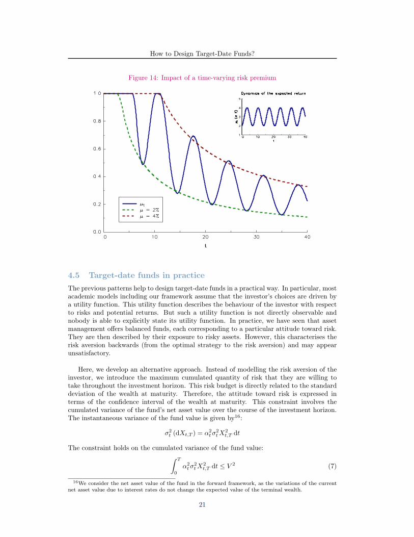
4.4 The importance of tactical asset allocationIn the previous paragraphs, we assume that the risk premium and the volatility of the riskyasset are constant. In real life, however, this is not the case. For example, the volatilityof the equity market exhibits some regimes or may be viewed as a mean-reverting process.Since the work of Lucas (1978), we know that risk premia are time-varying. In particular,we observe a covariance effect with the consumption behaviour of investors due to the factthat output exhibits some cycle (Darolles et al., 2010). In this context, defining a glide pathwith a constant risk premium and a constant volatility is suboptimal.

Suppose for example that the expected return of the risky asset is given by a sine function:

µt = 3%+ 1% · sin(2π

7(T − t)

)It implies that the expected return varies between 2% and 4% and that the cycle period is7 years. We have illustrated the corresponding glide path in Figure 14. We observe thatthe glide path is located between two curves, which are the glide paths for the lower andupper bounds of µt. The variations may be very large. For example, if t is equal to 11years, the optimal exposure is 100% while it becomes 30% three years later. If we assumethat the volatility is time-varying, we obtain similar conclusions. In finance, we generallyobserve that performance is negatively correlated to risk. It is especially true for equities. Inthis case, we will have a double effect: a negative outlook on expected return will decreasethe optimal exposure, and this jump will be amplified because of the increase in volatility.Taking into account the short-run behaviour of asset classes is also necessarily in orderto optimise the glide path. Using strategic asset allocation to estimate the long-run pathof financial assets in terms of performance and risk is insufficient and therefore must besupplemented by tactical asset allocation.

20


Figure 14: Impact of a time-varying risk premium

4.5 Target-date funds in practiceThe previous patterns help to design target-date funds in a practical way. In particular, mostacademic models including our framework assume that the investor’s choices are driven bya utility function. This utility function describes the behaviour of the investor with respectto risks and potential returns. But such a utility function is not directly observable andnobody is able to explicitly state its utility function. In practice, we have seen that assetmanagement offers balanced funds, each corresponding to a particular attitude toward risk.They are then described by their exposure to risky assets. However, this characterises therisk aversion backwards (from the optimal strategy to the risk aversion) and may appearunsatisfactory.

Here, we develop an alternative approach. Instead of modelling the risk aversion of theinvestor, we introduce the maximum cumulated quantity of risk that they are willing totake throughout the investment horizon. This risk budget is directly related to the standarddeviation of the wealth at maturity. Therefore, the attitude toward risk is expressed interms of the confidence interval of the wealth at maturity. This constraint involves thecumulated variance of the fund’s net asset value over the course of the investment horizon.The instantaneous variance of the fund value is given by16:

σ2t (dXt,T ) = α2

tσ2tX

2t,T dt

The constraint holds on the cumulated variance of the fund value:∫ T

0

α2tσ

2tX

2t,T dt ≤ V 2 (7)

16We consider the net asset value of the fund in the forward framework, as the variations of the currentnet asset value due to interest rates do not change the expected value of the terminal wealth.

21


where V 2 is the total variance budget of the strategy from inception date to maturity.Once the risk has been constrained, the investor can focus on achieving the highest possibleaverage return. This is a translation of Markowitz problem in a dynamical framework. Theobjective is to maximise the expected wealth at maturity, under the constraint (7):

α∗t = argmaxE0 [XT ] such that

∫ T

0

α2tσ

2tX

2t,T dt ≤ V 2

We suppose that the Sharpe ratio of the forward price St,T of the risky asset is constant,and that the interest rates are deterministic. In this case, the optimal allocation policy isgiven by:

α∗t =

V

σt

√TXt,T

The optimal proportion of risky assets is a linear function of the total risk budget V , andit is inversely proportional to the forward wealth and the volatility of the risky asset. Letv⋆ = V/E [Xt] be the risk budget expressed in terms of the terminal wealth. The glidepath may be approximated by the following system if we assume that the sharpe ratioSR = (µt − rt) /σt is constant:

gt =V

σt

√Txt

dxt =V

xtSR dt+ πt dt (8)

xt = v⋆xT

We could then use a classical optimisation algorithm and the Runge-Kutta method to de-termine the glide path gt, the associated expected wealth xt and the risk budget V .

Let us consider our previous example defined in Section 3.3 page 12. We assume thatµ = 3%, σ = 15% and r = 1%. In Figure 15, we have reported in the first panel theglide path17 corresponding to different values of the risk budgeting ratio v⋆. For example,v⋆ = 10% corresponds to a volatility budget V equal to USD 82 600. In this case, XT takesthe value USD 826 00018. If the investor finds this volatility budget V too high, they couldreduce it by choosing a smaller value for v⋆. For example, he could fix v⋆ to 1% implyingthat the risky exposure is largely reduced. In the second panel, we show the influence of thecontribution function. Please note that our results are based on an initial wealth X0 equalto USD 10 000 and a cumulative contribution Π0 close to USD 800 000. If the contributionis divided by a factor of 10, we observe a significant impact on the risky exposure. Finally,the last panel illustrates the relationship between the glide path and the parameters of therisky asset. In the previous theoretical model, an increase of µ is equivalent to a decreasein σ. In this practical model, it is not the case, because of the risk budget constraint. Thismodel then has an appealing property, because it contains a volatility target mechanism.

From a professional point of view, the model (8) is more powerful than the theoreticalmodel based on the Merton approach, because the results are quite similar to the glidepaths obtained via the utility framework although it is more tractable. Moreover, insteadof relying on an abstract risk aversion parameter, it uses an explicit standard deviationparameter V , which is the risk budget of the investor. Finally, we could easily extend themodel by considering tactical asset allocation.

17with a maximum exposure of 100%18We verify that the ratio between V and XT is 10%.

22


Figure 15: Glide path with the risk budgeting approach

5 Conclusion

This paper proposes a model to understand the design of target-date funds. Our model isbased on the seminal work of Merton (1969, 1971) in which we introduce stochastic interestrates and stochastic contribution. We show that the optimal exposure to risky assets couldbe obtained by solving a two-dimensional PDE. We illustrate the impact of the differentparameters such as the risk premium or the volatility of the risky asset, the correlationsbetween the risky asset, the interest rate and the savings component, etc. We notice that themost important factors for designing a target-date fund relate to the investors’ parameters:retirement date, level of risk aversion and income perspective.

This paper highlights the role of the glide path. In the investment industry, these glidepaths are defined on creation of the target-date fund and are hardly revisited. By analysingthe theoretical behaviour of the solution, we find that defining the optimal exposure issomewhere equivalent to defining a risk budget path. This is why we propose to designtarget-date funds by using a glide path, not in terms of weighting but rather in terms ofrisk19. This practical solution has the advantage of encompassing the risk aversion of theindividual and verifying the target risk pattern.

Our model may be improved in three ways. First, we assume that the retirement date isconstant. Introducing a stochastic retirement date is more realistic for two reasons: ageingpopulation in developed countries forces governments to delay retirement20 and the joblessof individuals in their fifties or sixties imply that they will use perhaps their pension savings

19This approach is related to risk parity portfolios defined in Maillard et al. (2010) and Bruder andRoncalli (2012).

20See Lachance (2008) for an example of a lifecycle model with a stochastic retirement date.

23


before their retirement date. Second, our model assumes that retirement is the maturity ofthe optimization problem. By assuming that, we ignore how many years the individual willlive after retirement and if the pension benefits will be sufficient, especially if the individuallives a long time. A more realistic model consists then in considering the financial life ofthe individual after the retirement date. Last, but not least, the investment policy of theindividual does not take the housing problem (Kraft and Munk, 2011) into consideration.This last issue leads to a fundamental question for individuals: how will renting or owningresidential real estate modify optimal exposure to risky assets?

24


A Mathematical results

A.1 Forward dynamics

We have:

St,T =St

Bt,T

=S0

B0,Texp

(∫ t

0

(µu − ru − 1

2

(σ2u − Γ2

u,T

))du+

∫ t

0

σu dWSu − Γu,T dWB

u

)St,T is then a log-normal process and could be written as follows:

St,T = S0,T exp

(∫ t

0

(µu,T − 1

2σ2u,T

)du+

∫ t

0

σu,T dBSu

)By construction, BS

t is a brownian motion and we have:

σ2t,T dt = var

(σtW

St − Γt,TW

Bt

)=

(σ2t + Γ2


)dt

It implies that:

µt,T = µt − rt −1

2

(σ2t − Γ2

t,T

)+

1

2σ2t,T

= µt − rt + Γ2t,T − ρS,BσtΓt,T

In a similar way, we deduce that Qt,T is a log-normal process:

Qt,T = Q0,T exp

((θt,T − 1

2ζ2t,T

)t+ ζt,TB

Qt

)with: {

θt,T = θt,T − rt + Γ2t,T − ρQ,BζtΓt,T

ζt,T =√ζ2t + Γ2


Let ρ⋆ be the correlation between the two brownian motions BSt and BQ

t . It satisfies thefollowing relationship:

⟨dSt,T ,dQt,T ⟩ = ρ⋆σt,T ζt,T dt

We have also:

ρ⋆σt,T ζt,T dt =⟨σtdW

St − Γt,TdW

Bt , ζtdW

Qt − Γt,TdW

Bt

⟩=

(ρS,Qσtζt − ρQ,BζtΓt,T − ρS,BσtΓt,T + Γ2

t,T

)dt

We deduce that:

ρ⋆ =ρS,Qσtζt − ρQ,BζtΓt,T − ρS,BσtΓt,T + Γ2

t,T√σ2t + Γ2


√ζ2t + Γ2


25


A.2 Solving the HJB equationLet J be the function defined by:

J (t, x, q) = supα

Et [U (XT ) | Qt,T = q,Xt,T = x]

We may show that J verifies the following HJB equation (Pham, 2009, Prigent, 2007):

∂tJ (t, x, q) + maxα

H (t, x, q, α) = 0

where H is the associated Hamiltonian:

H (t, x, q, α) = (αµt,Tx+ ptq) ∂xJ (t, x, q) + θt,T q∂qJ (t, x, q) +

1

2α2σ2

t,Tx2∂2

xJ (t, x, q) + αρ⋆σt,T ζt,Txq∂2x,qJ (t, x, q) +

1

2ζ2t,T q

2∂2qJ (t, x, q)

At the optimum, we have:

∂H (t, x, q, α)

∂ α= µt,TxJ (t, x, q) + ασ2

t,Tx2∂2

xJ (t, x, q) +

ρ⋆σt,T ζt,Txq∂2x,qJ (t, x, q)

= 0

We deduce that the optimal exposure is:

α∗t = −

µt,T∂xJ (t, x, q) + ρ⋆σt,T ζt,T q∂2x,qJ (t, x, q)

xσ2t,T∂

2xJ (t, x, q)

The HJB equation becomes a two-dimensional PDE:

∂tJ (t, x, q) +H (t, x, q, α∗t ) = 0 (9)

From a numerical point of view, the HJB equation (9) is solved on the space [x−, x+]×[q−, q+] with t ∈ [0, T ]. We impose boundary on the allocation such that 0 ≤ αt ≤1. For the boundary conditions, we assume that J (T, x, q) = U (x), ∂qJ (t, x, q−) =∂qJ (t, x, q− + dq), ∂qJ (t, x, q+) = ∂qJ (t, x, q+ − dq), ∂xJ (t, x−, q) = x−

γ−1∂2xJ (t, x−, q)

and ∂xJ (t, x+, q) =x+

γ−1∂2xJ (t, x+, q). We consider that q− = 0 and q+ = 2 whereas the

bounds x− and x+ depend on the initial wealth and the expected future contribution ofthe investor. For our example, we have taken x− ≃ 0 and x+ = 2 × 106. We then use theHopscotch algorithm to solve the HJB equation numerically (Kurpiel and Roncalli, 1999).

A.3 Derivation of the relationship (5)Without interest rates and uncertainty of savings (πt = pt), the dynamics of the wealthbecomes:

dXπt

Xπt

= αtdSt

St

with Xπt = Xt +

∫ T

tπu du and αt = αtXt/X

πt . It comes that:

Xπt = Xπ

0 exp

(∫ t

0

(αuµu − 1

2α2uσ

2u

)du+

∫ t

0

αuσu dBu

)26


With U (x) = xγ/γ, we have:

maxαt

Et [U (XπT )] ⇔ max

αt

γ

(αtµt −

1

2α2tσ

2t

)+

1

2γ2α2

tσ2t

The optimal solution is then:α⋆t =

µt

(1− γ)σ2t

or:

α⋆t =

µt

(1− γ)σ2t

(1 +

∫ T

tπu du

x

)

A.4 Computation of the glide path when the contribution functionis linear

Let mt = E [Xt]. If πt is deterministic, we have:

dmt = αtµmt dt+ πt dt

= αµmt dt+

(αµ

∫ T

t

πu du+ πt

)dt

In the case where πt = at+ b, It comes that:

dmt = αµmt dt+

(αµ

[1

2au2 + bu

]Tt

+ at+ b

)dt

= αµmt dt+

(αµ

(1

2a(T 2 − t2

)+ b (T − t)

)+ at+ b

)dt

and:

mt = x0eαµt + αµ

(1

2aT 2 + bT

)t− αµ

(1

6at2 +

1

2bt

)t+

(1

2at+ b

)t

If the wealth is sufficient high21, we have :

gt ≃ α+µ(12a(T 2 − t2

)+ b (T − t)

)(1− γ)σ2mt

A.5 Impact of the correlations on optimal exposure

We notice that the correlation parameters ρS,Q, ρS,B and ρQ,B influence the optimal solutionα⋆t because they modify the forward correlation ρ⋆. So, if we are able to quantify the impact

of ρ⋆, we are able to analyse the impact of these correlation parameters.

Let us first consider the relationship (1) between the correlation parameters and theforward correlation. We consider the previous values of parameters: σt = 15%, ζt = 3%and T = 40 years. In Figure 16, we have reported the value of ρ⋆ with respect to time tfor three values of ρS,Q. If φ is set to zero and if there is not correlation between the riskyasset St and the economic factor Qt or the bond Bt,T , ρ⋆ is exactly equal to ρS,Q. If φ

21in order to diminish the convexity effect in Jensen’s inequality.

27


increases, the correlation ρ⋆ increases too. In particular22, we have ρ⋆ → ρS,Q when t → T ,ρ⋆ ≥ ρ⋆ when t → 0 and ρ⋆ → 1 when t → 0 and φ → ∞. These behaviors are illustratedin the second and third panels in Figure 16, whereas the impact of ζt is reported in thefourth panel. Figures 17 and 18 shows how the forward correlation changes with respect tothe correlations ρS,B and ρQ,B. The forward correlation is a decreasing function of thesetwo parameters, but the impact depend on the respective magnitude of the volatility of Qt,Bt, T and St. It explains that the impact of ρQ,B is small in Figure 18.

Figure 16: The case ρS,B = ρS,Q = 0

Because J (t, x, q) is a utility function, we could assume that ∂xJ (t, x, q) ≥ 0 and∂2xJ (t, x, q) ≤ 0. Another expression of the equation (2) is:

α∗t,x =

µt,T

σ2t,T

(− ∂xJ (t, x, q)

x∂2xJ (t, x, q)

)− ρ⋆

ζt,Tσt,T

(q∂2

x,qJ (t, x, q)

x∂2xJ (t, x, q)

)

=1

R (t, x, q)

µt,T

σ2t,T

− ρ⋆1

Ex (t, x, q)ζt,Tσt,T

where R (t, x, q) ≥ 0 is the relative risk aversion and Ex (t, x, q) ≥ 0 is a function whichdepends on the derivatives of the marginal utility. It comes that:

∂ α∗t,x

∂ ρ⋆≤ 0

22In the case ρS,B = ρQ,B = 0, the formula (1) reduces to:

ρ⋆ =ρS,Qσtζt + φ2T 2√

σ2t + φ2T 2

√ζ2t + φ2T

28


Figure 17: The case φ = 20 bps

Figure 18: The case φ = 1%

29


References[1] Bajeux-Besnainou I., Jordan J.V. and Portait R. (2003), Dynamic Asset Alloca-

tion for Stocks, Bonds, and Cash, Journal of Business, 76(2), pp. 263-287.

[2] Barberis N. (2000), Investing for the Long Run When Returns Are Predictable, Jour-nal of Finance, 55(1), pp. 225-264.

[3] Basu A. and Drew M.E. (2009), Portfolio Size Effect in Retirement Accounts: Whatdoes it imply for Lifecycle Asset Allocation Funds?, Journal of Portfolio Management,35(3), pp. 61-72.

[4] Bodie Z. (2003), Life-Cycle Investing in Theory and Practice, Financial Analysts Jour-nal, 59, pp. 24-29.

[5] Bodie Z., Merton R. and Samuelson W.F. (1992), Labor Supply Flexibility andPortfolio Choice in a Life Cycle Model, Journal of Economic Dynamics and Control,16(3-4), pp. 427-449.

[6] Bodie Z., Detemple J.B., Otruba S. and Walter S. (2004), Optimal Consumption-Portfolio Choices and Retirement Planning, Journal of Economic Dynamics and Con-trol, 28(6), pp. 1115-1148.

[7] Bodie Z., Detemple J. and Rindisbacher M. (2009), Life Cycle Finance and theDesign of Pension Plans, www.ssrn.com/abstract=1396835.

[8] Booth P. and Yakoubov Y. (2000), Investment Policy for Defined-Contribution Pen-sion Scheme Members close to Retirement: An Analysis of the Lifestyle Concept, NorthAmerican Actuarial Journal, 4(2), pp. 1-19.

[9] Brennan M.J. and Xia Y. (2002), Dynamic Asset Allocation under Inflation, Journalof Finance, 57(3), pp. 1201-1238.

[10] Bruder B., Jamet G. and Lasserre G. (2010), Beyond Liability-Driven Investment:New Perspectives on Defined Benefit Pension Fund Management, Lyxor White PaperSeries, 2, www.lyxor.com.

[11] Bruder B. and Roncalli T. (2012), Managing Risk Exposures using the Risk Bud-geting Approach, Working Paper, www.ssrn.com/abstract=2009778.

[12] Campbell J.Y. (2000), Asset Pricing at the Millennium, Journal of Finance, 55(4),pp. 1515-1567.

[13] Campbell J.Y., Cocco J., Gomes F., Maenhout P.J. and Viciera L.M. (2001),Stock Market Mean Reversion and the Optimal Equity Allocation of a Long-LivedInvestor, Review of Finance, 5(3), pp. 269-292.

[14] Campbell J.Y. and Viciera L.M. (2002), Strategic Asset Allocation, Oxford Univer-sity Press.

[15] Canner N., Mankiw N.G. and Weil D.N. (1997), An Asset Allocation Puzzle, Amer-ican Economic Review, 87(1), pp. 181-191.

[16] Cochrane J.H. (2001), Asset Pricing, Princeton University Press.

[17] Cocco J.F. and Gomes F.J. (2012), Longevity Risk, Retirement Savings, and FinancialInnovation, Journal of Financial Economics, 103(3), pp. 507-529.

30


[18] Cocco J.F., Gomes F.J. and Maenhout P.J. (2005), Consumption and PortfolioChoice over the Life Cycle, Review of Financial Studies, 18(2), pp. 491-533.

[19] Darolles S., Eychenne K. and Martinetti S. (2010), Time Varing Risk Premiums& Business Cycles: A Survey, Lyxor White Paper Series, 4, www.lyxor.com.

[20] Geman H., El Karoui N. and Rochet J-C. (1995), Changes of Probability Measureand Option Pricing, Journal of Applied Probability, 32(2), pp. 443-458.

[21] Eychenne K., Martinetti S. and Roncalli T. (2011), Strategic Asset Allocation,Lyxor White Paper Series, 6, www.lyxor.com.

[22] Gomes F. and Michaelides A. (2005), Optimal Life-Cycle Asset Allocation: Under-standing the Empirical Evidence, Journal of Finance, 60(2), pp. 869-904.

[23] Henderson V. (2005), Explicit Solutions to an Optimal Portfolio Choice Problem withStochastic Income, Journal of Economic Dynamics and Control, 29(7), pp. 1237-1266.

[24] Ho T.S.Y. and Lee S-B. (1986), Term Structure Movements and Pricing Interest RateContingent Claims, Journal of Finance, 41(5), pp. 1011-1029.

[25] Ilmanen A. (2003), Stock-Bond Correlations, Journal of Fixed Income, 13(2), pp. 55-66.

[26] INSEE (2006), Épargne et Patrimoine des Ménages, L’Économie Française,www.insee.fr/fr/ffc/docs_ffc/ecofrac06c.pdf.

[27] Investment Company Institute (2012), Investment Company Fact Book – A Reviewof Trends and Activity in the U.S. Investment Company Industry, 52nd edition,www.icifactbook.org.

[28] Jagannathan R. and Kocherlakota N.R. (1996), Why Should Older People In-vest Less in Stocks Than Younger People?, Quarterly Review, Federal Reserve Bank ofMinneapols, 20(3), pp. 11-23.

[29] Kraft H. and Munk C. (2011), Optimal Housing, Consumption, and InvestmentDecisions over the Life Cycle, Management Science, 57(6), pp. 1025-1041.

[30] Kurpiel A. and Roncalli T. (2000), Hopscotch Methods for Two State FinancialModels, Journal of Computational Finance, 3/2, pp. 53-89.

[31] Lachance M-E. (2008), Pension Reductions: Can Welfare be Preserved by DelayingRetirement?, Journal of Pension Economics and Finance, 7(2), pp. 157-177.

[32] Larsen L.S. and Munk C. (2012), The Costs of Suboptimal Dynamic Asset Allocation:General Results and Applications to Interest Rate Risk, Stock Volatility Risk, andGrowth/Value Tilts, Journal of Economic Dynamics and Control, 36(2), pp. 266-293.

[33] Lucas R.E. (1978), Asset Prices in an Exchange Economy, Econometrica, 46(6), pp.1429-1445.

[34] Maillard S., Roncalli T. and Teiletche J. (2010), The Properties of EquallyWeighted Risk Contributions Portfolios, Journal of Portfolio Management, 36(4), pp.60-70.

[35] Markowitz H. (1952), Portfolio Selection, Journal of Finance, 7(1), pp. 77-91.

31


[36] Martellini L. and Milhau V. (2010), From Deterministic to Stochastic Life-Cycle In-vesting: Implications for the Design of Improved Forms of Target Date Funds, EDHEC-Risk Institute Publication.

[37] Merton R.C. (1969), Lifetime Portfolio Selection under Uncertainty: The Continuous-Time Case, Review of Economics and Statistics, 51(3), pp. 247-257.

[38] Merton R.C. (1971), Optimum Consumption and Portfolio Rules in a Continuous-Time Model, Journal of Economic Theory, 3(4), pp. 373-413.

[39] Morningstar Fund Research (2012), Target-Date Series Research Paper: 2012 IndustrySurvey, corporate.morningstar.com.

[40] Munk C. and Sørensen C. (2010), Dynamic Asset Allocation with Stochastic Incomeand Interest Rates, Journal of Financial Economics, 96(3), pp. 433-462.

[41] Munk C., Sørensen C. and Vinther T.N. (2004), Dynamic Asset Allocation underMean-reverting Returns, Stochastic Interest Rates and Inflation Uncertainty: Are Pop-ular Recommendations Consistent with Rational Behavior?, International Review ofEconomics and Finance, 13(2), pp. 141-166.

[42] Pham H. (2009), Continuous-time Stochastic Control and Optimization With FinancialApplications, Stochastic Modeling and Applied Probability Series, 61, Springer.

[43] Prigent J.-L. (2007), Portfolio Optimization and Performance Analysis, Chapman &Hall.

[44] Quinn J.B. (1991), Making the Most of Your Money, Simon and Schuster.

[45] Poterba J., Rauh J., Venti S. and Wise D. (2009), Lifecycle Asset Allocation Strate-gies and the Distribution of 401(k) Retirement Wealth, in D. Wise (ed.), Developmentsin the Economics of Aging , University of Chicago Press, pp. 15-50.

[46] Shiller R.J. (2006), Life-Cycle Personal Accounts Proposal for Social Security: AnEvaluation of President Bush’s Proposal, Journal of Policy Modeling, 28, pp. 427-444.

[47] Viceira L.M. (2001), Optimal Portfolio Choice for Long-Horizon Investors with Non-tradable Labor Income, Journal of Finance, 56(2), pp. 433-470.

[48] Wachter, J.A. (2002), Portfolio and Consumption Decisions under Mean-RevertingReturns: An Exact Solution for Complete Markets, Journal of Financial and Quanti-tative Analysis, 37(1), pp. 63-91.

32

how to design target-date funds? - thierry roncallithierry-roncalli.com/download/lwp-tdf.pdf · how...

Documents