• Discrete Fourier Transform (in short, DFT)

• Remember we have introduced three kinds of Fourier transforms.

• However, what we are able to deal with in the discrete-time domain is usually a finite-duration signal.

• DFT is the final (fourth) Fourier transform, where its input is a discrete-time finite-duration signal.

How to manipulate Frequencies in Discrete-time Domain?

Two Main Approaches

Details will be introduced in later courses

• Difference Equations (an LTI system, Z-transform)

x[n]: input, y[n]: output

• That is, building a system that

makes use of the current and previous inputs x[n], x[n-1], x[n-2] …. as well as the previous outputs y[n-1], y[n-2], …

What is Spectrum in general?

• Remember that there are four kinds of Fourier transforms.

• What is the one that defines generally the concept of “spectrum?”

• Answer: The continuous Fourier transform (CFT) defines the spectrum in general.

• CFT pair

dtetfjwF

jwt

dwejwFtfjwt

2

1

Recall: Sampling for Processing

• In DSP, we always have to sample continuous-time (analog) signals into discrete-time signals for processing.

• Sampling in time domain: remember that if we perform sampling on an analog signal xa,

• Sampling in frequency domain: the spectrum becomes the sum of infinite many shifted copies of the original spectrum,

1 2

s a

r

rX jw X jw j

T T

( ) ( ) ( )s a

n

x t x nT t nT

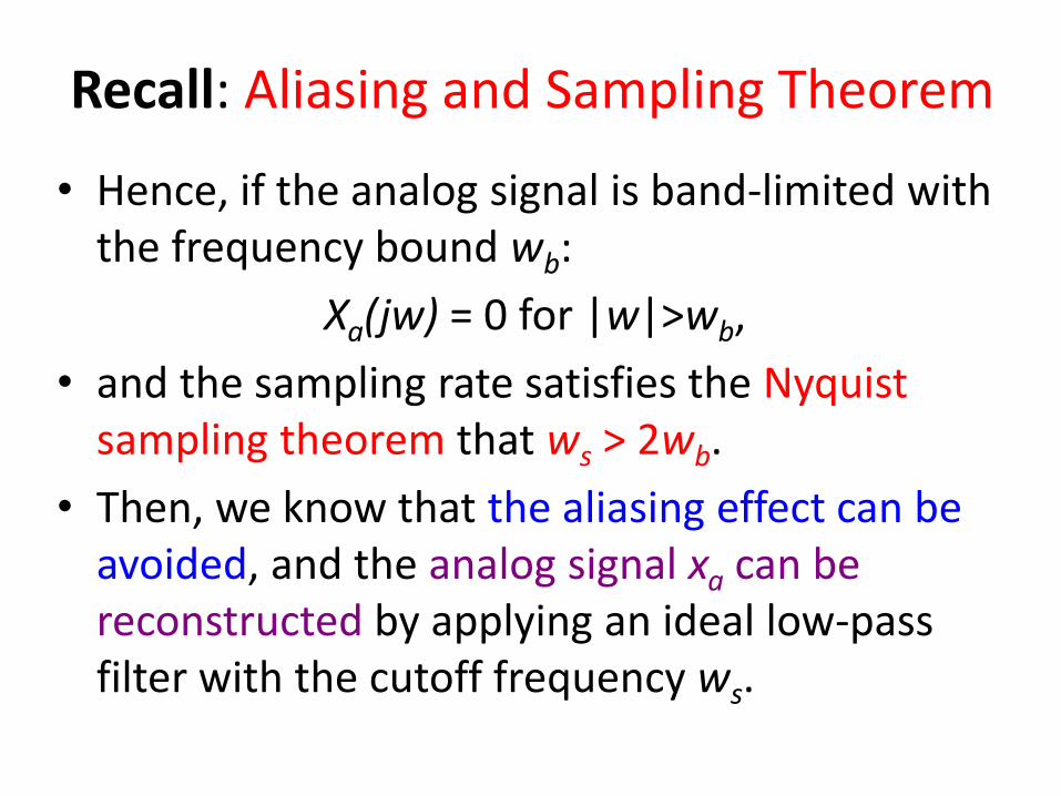
Recall: Aliasing and Sampling Theorem

• Hence, if the analog signal is band-limited with the frequency bound wb:

Xa(jw) = 0 for |w|>wb,

• and the sampling rate satisfies the Nyquist sampling theorem that ws > 2wb.

• Then, we know that the aliasing effect can be avoided, and the analog signal xa can be reconstructed by applying an ideal low-pass filter with the cutoff frequency ws.

Continuous signal Sampled signal

The magnitude spectrum of the continuous signal The spectrum of the sampled signal

Recall: Exact Reconstruction (without aliasing)

Recall: Why using DTFT • Since we have always to deal with discrete-time

signals in DSP, we have defined a Fourier transform, DTFT, particularly for discrete-time signal processing.

• DTFT pair:

• The spectrum of DTFT is defined in [-, ], and is periodic in the frequency domain with the period 2 (repeated when w w+2).

dweeXnx

jwnjw

2

1

n

jwnjwenxeX

Recall: How DTFT approximates CFT?

• If x[n] is sampled from the analog signal xa(t) with x[n]=xa(nT),

• and remember in the analog domain, these samples are represented as

• Relationship between X(ejw) (i.e., the DTFT of x[n]) and Xs(jw) (i.e., the CFT of xs(t)) is

• That is, Xs(jw) can be obtained by simply stretching X(ejw) with wwT.

• Xs(jw) is a periodic function in w with the period 2/T, and a single period within [-/T, /T].

)( jwXeXs

jwT

( ) ( ) ( )s a

n

x t x nT t nT

Recall: How DTFT approximates CFT? • More specifically, we have the relationship between X(ejw) (i.e.,

the DTFT of x[n]) and Xa(jw) (i.e., the CFT of xa(t)) as

• Exact recovery: when the Xa(jw) is band-limited and the sampling rate is high enough such that the sampling theorem is satisfied, Xa(jw) can be exactly recovered from the DTFT X(ejwT) (by investigating the range only in w[-/T, /T ]).

• Approximation: When the sampling rate is not high enough or Xa(jw) is not band-limited, X(ejwT) is only an approximation of Xa(jw) because of the aliasing effect (some high-frequency part will be folded to the range [-/T, /T ]).

• How DTFT approximates CFT can be completely characterized by sampling theorem and aliasing effect.

r

as

jwT

T

rjjwX

TjwXeX )

2(

1)(

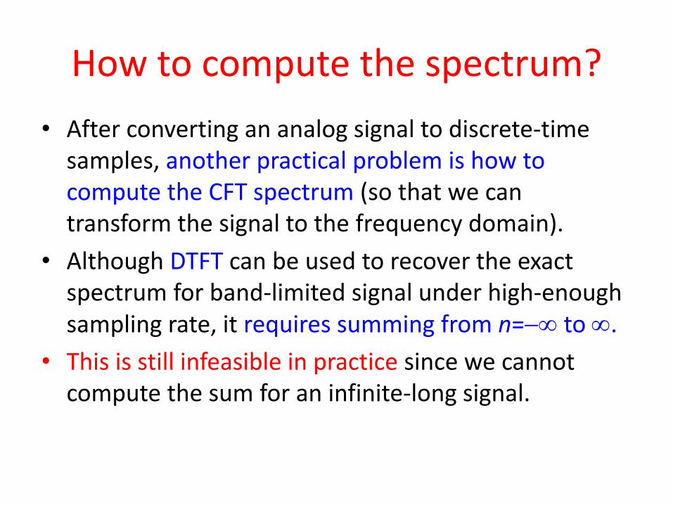
How to compute the spectrum?

• After converting an analog signal to discrete-time samples, another practical problem is how to compute the CFT spectrum (so that we can transform the signal to the frequency domain).

• Although DTFT can be used to recover the exact spectrum for band-limited signal under high-enough sampling rate, it requires summing from n= to .

• This is still infeasible in practice since we cannot compute the sum for an infinite-long signal.

Approximation by Finite-duration Signals

• So, what can we do? • A practical way commonly employed is to use a finite range t[-T/2,

T/2] of the analog signal xa(t), and see how it can approximate the spectrum of the entire signal defined in t(, ).

• After sampling with x[n]=xa(nT), there are N=T/T samples in the range t[-T/2, T/2], resulting a finite-duration discrete-time signal y[n] from x[n],

• Compute the DTFT for the finite-duration signal y[n] (now it is feasible in practice), and see how it can approximate the DTFT of x[n].

• We can expect that, the larger is N (or equivalently, the larger is the range T), the better is the approximated spectrum.

otherwise

Nnnxny

,0

10],[][

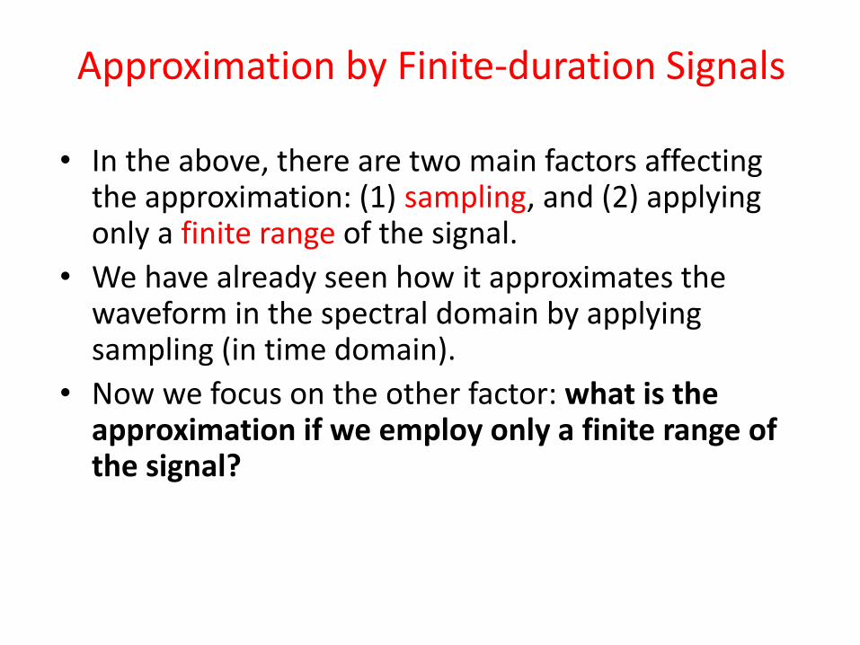
Approximation by Finite-duration Signals

• In the above, there are two main factors affecting the approximation: (1) sampling, and (2) applying only a finite range of the signal.

• We have already seen how it approximates the waveform in the spectral domain by applying sampling (in time domain).

• Now we focus on the other factor: what is the approximation if we employ only a finite range of the signal?

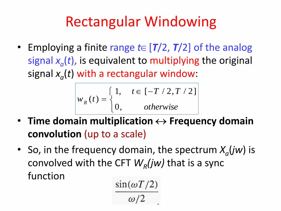
Rectangular Windowing

• Employing a finite range t[T/2, T/2] of the analog signal xa(t), is equivalent to multiplying the original signal xa(t) with a rectangular window:

• Time domain multiplication Frequency domain convolution (up to a scale)

• So, in the frequency domain, the spectrum Xa(jw) is convolved with the CFT WR(jw) that is a sync function

otherwise

TTttw

R,0

]2/,2/[,1)(

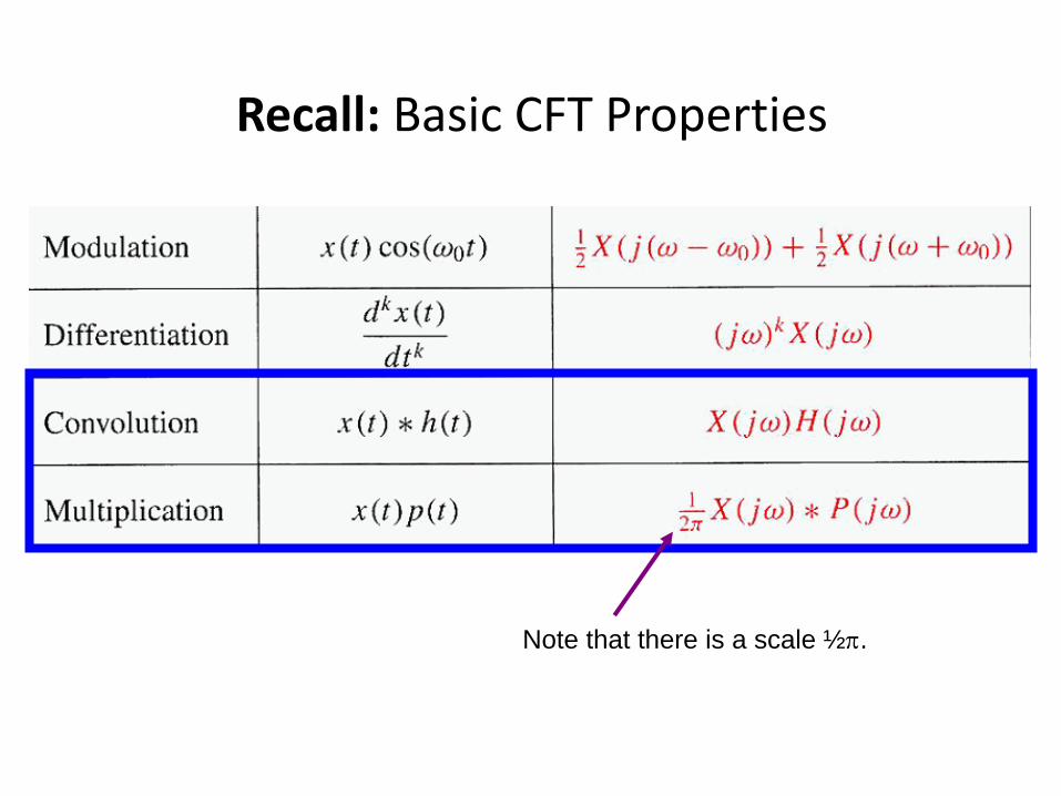
Recall: Basic CFT Properties

Note that there is a scale ½ .

Multiplication with a rectangular window in the analog domain

)(twR

Multiplication with the

rectangular window,

Convolution with the

following sync

function then divided

by 2,

Convolution with Sync Function

• What is the effect of convolution with a sync function?

• Note that when T (that is, wR(t) 1), the sync function approaches to the delta function 2(w).

• Convolution with a delta function and the divided by 2 recovers exactly the original spectrum.

w

Convolution with Sync Function

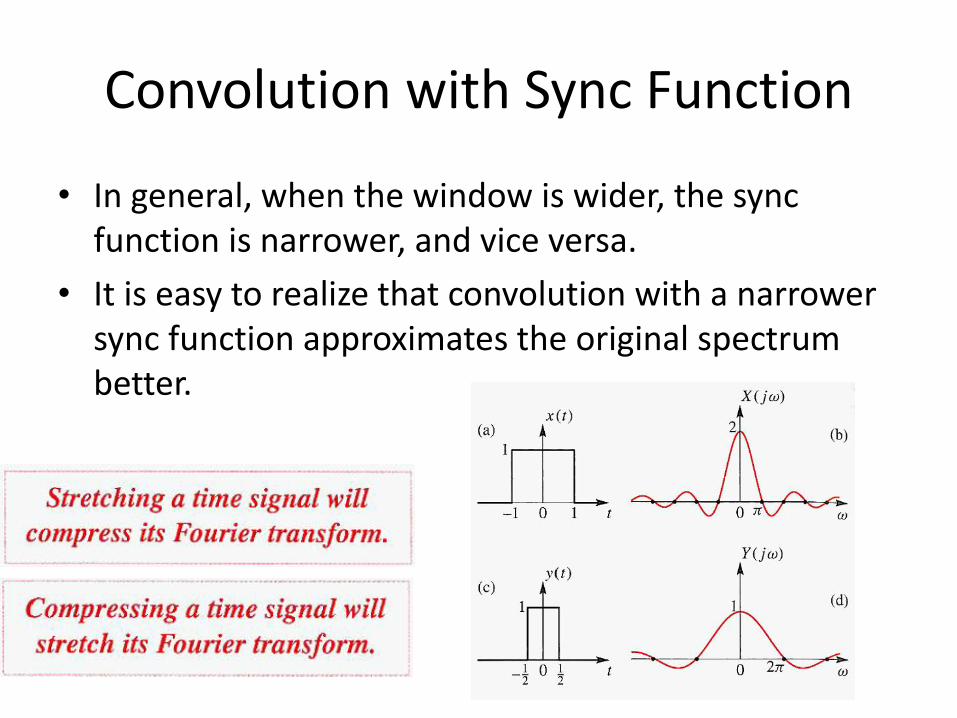
• In general, when the window is wider, the sync function is narrower, and vice versa.

• It is easy to realize that convolution with a narrower sync function approximates the original spectrum better.

Example: approximation for a single sinusoid

• Assume that there is a single sinusoidal signal applied by the rectangular window in time domain:

• Let us consider the magnitude response of the sync function:

Example: approximation for a single sinusoid

• Then, convolution of a spectrum of a single sinusoid with the sync function looks like

Approximation by rectangular windowing in the Analog domain

• It can be seen that, by using a finite-length portion of an analog signal, the approximation can be analyzed by convolving a sync function in the frequency domain.

• This convolution disturbs the original spectrum: the spectrum is blurred and somewhat oscillated.

• The narrower is the sync function (i.e., the longer is the window), the more accurate is the approximation.

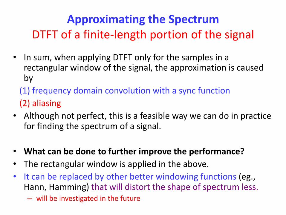
Approximating the Spectrum DTFT of a finite-length portion of the signal

• In sum, when applying DTFT only for the samples in a rectangular window of the signal, the approximation is caused by

(1) frequency domain convolution with a sync function

(2) aliasing

• Although not perfect, this is a feasible way we can do in practice for finding the spectrum of a signal.

• What can be done to further improve the performance?

• The rectangular window is applied in the above.

• It can be replaced by other better windowing functions (eg., Hann, Hamming) that will distort the shape of spectrum less. – will be investigated in the future

Spectrogram

• In the above, we only use a single segment of the signal and compute its DTFT.

• It is natural to extend this idea by separating a signal into multiple segments in time, and compute the DTFT for each segment along the time axis.

• In this way, we can obtain a two-dimensional map, where the horizontal axis is time index of the segment, and the vertical axis is the frequency in [-/T, /T].

• Spectrogram is the common way for viewing the spectral domain response for a signal in practice.

Spectrogram Examples

Synthesized notes, C,D,E,F,G,A,B,C Spectrogram of Fur Elise played on

a piano

Spectrogram Examples

Further Improvement

• In the above, we compute the DTFT for a finite-length signal (of length N).

• To record the frequency domain of DTFT, we have to record a continuous function in the range of [-, ].

• However, to record exactly a continuous function in a digital device is difficult in practice.

Example of a finite-length x(n) and its DTFT X(ejw).

A finite-length signal

Its magnitude spectrum of DTFT

Its phase spectrum of DTFT

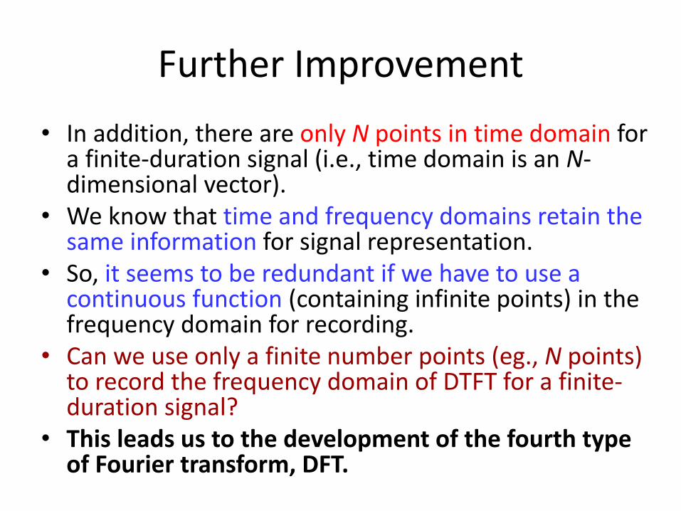
Further Improvement

• In addition, there are only N points in time domain for a finite-duration signal (i.e., time domain is an N-dimensional vector).

• We know that time and frequency domains retain the same information for signal representation.

• So, it seems to be redundant if we have to use a continuous function (containing infinite points) in the frequency domain for recording.

• Can we use only a finite number points (eg., N points) to record the frequency domain of DTFT for a finite-duration signal?

• This leads us to the development of the fourth type of Fourier transform, DFT.

DTFT of a discrete and periodic signal

• The DTFT spectrum of a discrete and periodic signal is also discrete and periodic.

A discrete-time periodic signal

Its magnitude spectrum (sampled)

Its phase spectrum (sampled)

Discrete Fourier Transform (DFT)

• Consider both the signal and the spectrum only within one period (N-point signals both in time and frequency domains)

where is a root of WN=1.

DFT

IDFT (inverse DFT)

NjeW

/2

From Kuhn 2005

DFT in matrix form

Relation between DFT and DTFT for finite-length signals

• The frequency coefficients of DFT are the N-point uniform samples of DTFT with [0, 2].

• The two equations DFT and IDFT give us a numerical algorithm to obtain the frequency response at least at the N discrete frequencies.

• Question: Can we reconstruct the DTFT spectrum (continuous in w) from the DFT?

• Since the N-length signal can be exactly recovered from both the DFT coefficients and the DTFT spectrum, we expect that the DTFT spectrum (that is within [0, 2]) can be exactly reconstructed by the DFT coefficients.

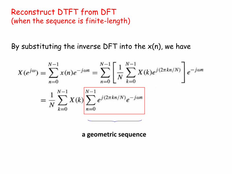
Reconstruct DTFT from DFT (when the sequence is finite-length)

By substituting the inverse DFT into the x(n), we have

a geometric sequence

By applying the geometric-sequence formula

magnitude

phase

So

The reconstruction formula From X(k), the spectrum of DFT , we can reconstruct the spectrum of DTFT, X(ejw) by the above interpolation.

Hence, instead of computing the DTFT of a finite-duration signal directly, we always use DFT for the computation, and the DTFT spectrum can be exactly reconstructed for any w.

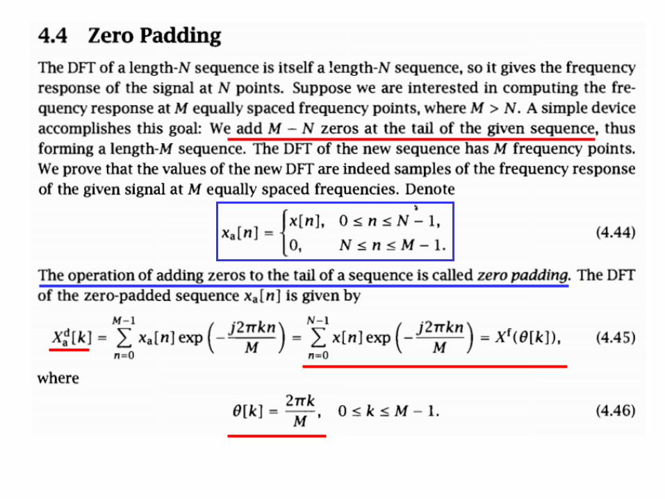
Another way to interpolate X(ejw) from X(k) is zero-padding

that will be shown below.

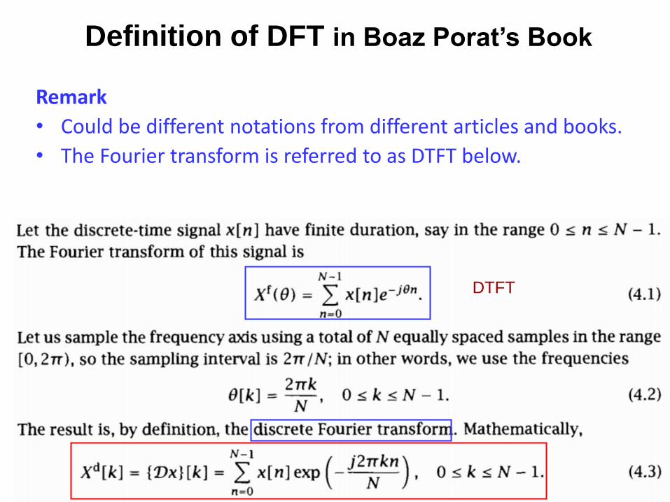
Definition of DFT in Boaz Porat’s Book

Remark

• Could be different notations from different articles and books.

• The Fourier transform is referred to as DTFT below.

DTFT

Fast Fourier Transform (FFT) An important characteristic of DFT is that it can be computed very fast DFT pairs:

WN = ej2/N is a root of the equation WN=1.

It requires N2 complex multiplications and (N1)N complex additions for direct computation.

1

0

1...,1,0 ,][][

N

n

kn

NNkWnxkX

1

0

1...,1,0 ,][1

][

N

k

kn

NNnWkX

Nnx

Decimation-in-time FFT algorithm

Most conveniently illustrated by considering the special case of N an integer power of 2, i.e, N=2v.

Since N is an even integer, we can consider computing X[k] by separating x[n] into two (N/2)-point sequence consisting of the even numbered point in x[n] and the odd-numbered points in x[n].

dd

][][][

on

nk

N

evenn

nk

NWnxWnxkX

Decimation-in-time FFT algorithm

With the substitution of variable n=2r for n even and n=2r+1 for n odd:

By the key property:

We have

1)2/(

0

)12(

1)2/(

0

2]12[]2[][

N

r

kr

N

N

r

rk

NWrxWrxkX

( / 2 ) 1 ( /2 ) 1

2 2

0 0

[ ] [2 ]( ) [2 1]( )

N N

rk k rk

N N N

r r

X k x r W W x r W

2/

)2//(2)/2(22

N

NjNj

NWeeW

( / 2 ) 1 ( /2 ) 1

/2 /2

0 0

[2 ]( ) [2 1]( )

N N

rk k rk

N N N

r r

x r W W x r W

In sum, • Both G[k] and H[k] can be computed by (N/2)-point DFT

• G[k]: the (N/2)-point DFT of the even numbered points of the original sequence

• H(k): the (N/2)-point DFT of the odd-numbered point of the original sequence.

• Although the index ranges over N values, k = 0, 1, …, N-1, they must be computed only for k between 0 and (N/2)-1, since G[k] and H[k] are each periodic in k with period N/2.

1,...,1,0 ],[][ NkkHWkGk

N

( / 2 ) 1 ( /2 ) 1

/2 /2

0 0

[ ] [2 ]( ) [2 1]( )

N N

rk k rk

N N N

r r

X k x r W W x r W

Decomposing N-point DFT into two (N/2)-point DFT for the case of N=8

We can further decompose the (N/2)-point DFT into two (N/4)-point DFTs. For example, the upper half of the previous diagram can be decomposed as

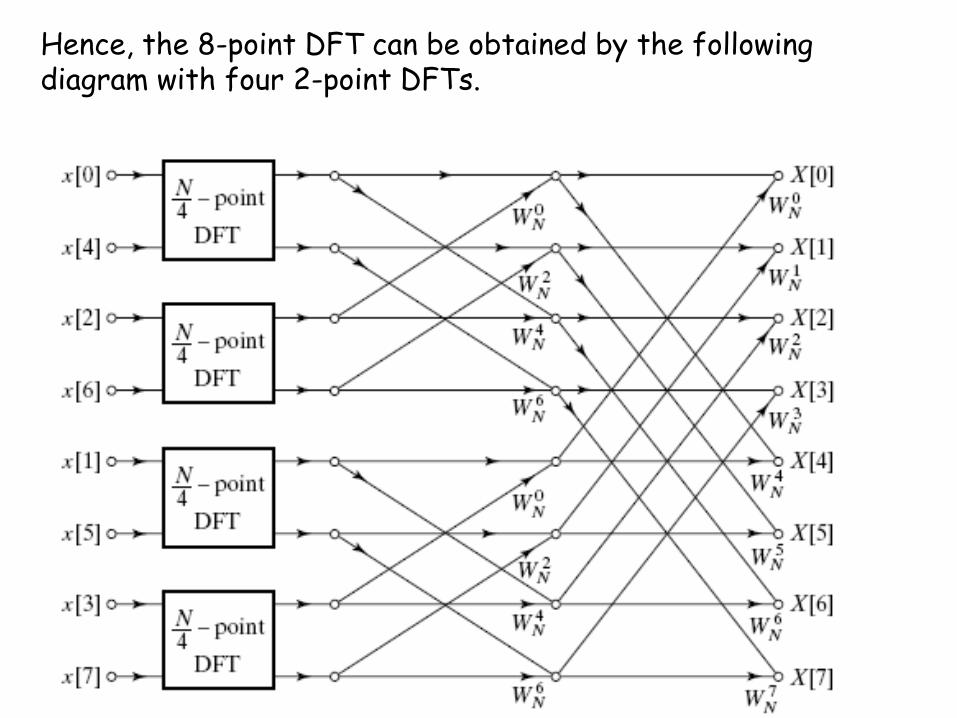
Hence, the 8-point DFT can be obtained by the following diagram with four 2-point DFTs.

Flow graph of a 2-point DFT

Finally, each 2-point DFT can be implemented by the following signal-flow graph, where no multiplications are needed.

Flow graph of complete decimation-in-time decomposition of an 8-point DFT.

In each stage of the decimation-in-time FFT algorithm, there are a basic structure called the butterfly computation: The butterfly computation can be simplified as follows:

Flow graph of a basic

butterfly computation in FFT.

Simplified butterfly computation.

][][][

][][][

11

11

qXWpXqX

qXWpXpX

m

r

Nmm

m

r

Nmm

Flow graph of 8-point FFT using the simplified butterfly computation

• In the above, we have introduced the decimation-in-time algorithm of FFT.

• Here, we assume that N is the power of 2. For N=2v, it requires v=log2N stages of computation.

• The number of complex multiplications and additions required was N+N+…N = Nv = N log2N.

• When N is not the power of 2, we can apply the same principle that were applied in the power-of-2 case when N is a composite integer. For example, if N=RQ, it is possible to express an N-point DFT as either the sum of R Q-point DFTs or as the sum of Q R-point DFTs.

• The FFT algorithm of power-of-two is also called the Cooley-Tukey algorithm since it was first proposed by them.