How You Export Matters: Export Mode,Learning and Productivity in China

Xue Bai, Kala Krishna and Hong Ma1

June 26, 2016

1Bai: Brock University, xbai@brocku.ca. Krishna: The Pennsylvania StateUniversity, NYU and NBER, kmk4@psu.edu. Ma: Tsinghua University, ma-hong@sem.tsinghua.edu.cn. Krishna is grateful to the Cowles Foundation at Yale and tothe Economics Department at NYU for support as a visitor, and to the World Bank forresearch support. The authors are grateful to the National Natural Science Foundation ofChina (NSFC) for support under Grant No. 71203114. We thank the China Data Cen-ter at Tsinghua University for access to the datasets. We are extremely grateful to MarkRoberts for his intellectual generosity and for sharing his codes with us. We also thankAndrew Bernard, Paula Bustos, Russell Cooper, Paul Grieco, Min Hua, Wolfgang Keller,Amit Khandelwal, Jicheng Liu, Chia Hui Lu, Nina Pavcnik, Joel Rodrigue, Daniel Tre-fler, James Tybout, Neil Wallace, Shang-Jin Wei, Adrian Wood, Stephen Yeaple, and JingZhang for extremely useful comments on an earlier draft. We would like to thank partici-pants at the Penn State-Tsinghua Conference on the Chinese Economy, 2012, the CES-IFOArea Conference on the Global Economy, 2012, the Midwest International Trade Meetings,2012, the Tsinghua-Columbia Conference in International Economics, 2012, the YokohamaConference, 2012, the NBER ITI spring meetings, 2013, the Penn State JMP conference,2013, the Cornell PSU Macro Conference, 2013, ERWIT, 2013, InsTED, 2013, PrincetonSummer Workshop, 2013 and the Yale International Trade workshop 2013, NBER ChineseEconomy Meeting 2014, Barcelona GSE Summer Forum 2014 for comments. We are alsograteful to seminar participants at the University of Virginia, Toronto, Toulouse, Paris, Na-mur, Kentucky, Brock, Auckland, and the City University of Hong Kong, Fudan University,BNU and CUFE for comments.

Abstract

This paper shows that how firms export (directly or indirectly via intermediaries)matters. We develop and estimate a dynamic discrete choice model that allowslearning-by-exporting on the cost and demand side as well as sunk/fixed costs todiffer by export mode. We find that demand and productivity evolve more favor-ably under direct exporting, though the fixed/sunk costs of this option are higher.Our results suggest that had China not liberalized its direct trading rights when itjoined the WTO, its exports and export participation would have been 26 and 33percent lower respectively.

Keywords. Export modes, Productivity evolution, Learning-by-exporting, Dy-namic discrete choice

1 Introduction

Firms can choose how they export: directly or indirectly through intermediaries.What are the costs and benefits of such choices? On the one hand, intermediariesprovide smaller firms the opportunity to engage in foreign trade without incurringthe many costs associated with direct exporting. On the other hand, indirect ex-porters face lower variable profits because intermediaries take a cut. The existingliterature on heterogeneous firms focuses on this static trade-off between export-ing directly and indirectly. However it neglects the dynamic trade-offs that mightexist if there were different learning-by-exporting effects for direct versus indirectexporters.

Learning-by-exporting refers to the mechanism whereby firms improve theirperformance (on the productivity and/or demand side) after entering export mar-kets. Case study evidence points to the importance of learning about cost-cuttingtechnologies and profit-boosting product designs through buyer-seller relationships.Egan and Mody (1992) give some examples of how direct engagement with buyersenhances learning. They say “importers are also more likely to employ designers,

engineers, and marketing experts who can provide technical assistance to suppli-

ers” and point to Schwinn, a well known brand in the US bicycle market, whichprovided technical assistance to its Chinese supplier to help it access the US mar-ket (see page 324). Regarding the footwear industry, they say that “Buyers may

assist sellers...by providing marketing information as to what products are selling

in a particular season and product specifications” (see page 328). Since firms whoexport through intermediaries usually do not engage in direct contact with their for-eign buyers and do not maintain employees in foreign markets, the pass-through ofknowledge may be less effective than that of direct exporters. Hence, firms whoexport directly may have more opportunities to improve than indirect ones. Con-sequently, firms’ current export mode choices can affect their future profits. Thesedynamic considerations can be vital in shaping the effects of policy.

In theory, learning effects could be bigger for indirect exporters than for directones: for example, it could be that indirect exporters acquire the cumulative knowl-edge of the intermediaries they are using. This may be particularly relevant in terms

1

of learning to deal with customs procedures and learning the ins and outs of howto get things done in settings where procedures are less transparent. Also, interme-diaries like Costco and Walmart may also provide significant input into what sortsof products to produce. These large intermediaries have vast experience about whatsells and often conduct a lot of market research that others could not. Thus, thequestion is an empirical one and one of the contributions of the paper is to see whatseems to hold in the data, at least for China.

Governments have long had a tendency to intervene in markets, often with whatthey see as the best of reasons. However, such interventions can have unanticipated,and often, detrimental effects.1 Before 2004, a large share of domestically ownedChinese firms were not allowed to trade directly,2 but these restrictions were relaxedas part of joining the WTO. Prior to the reform, they had to export only through in-termediaries unless their registered capital was quite large.3 If direct exporters learnmore than indirect ones, then limiting the ability to export directly could have hadsignificant adverse effects. We use this reform as a natural experiment and estimatea structural dynamic model that allows us to quantify the static and dynamic trade-offs and evaluate the cost of the restrictions on direct trading. We recover not onlythe sunk and fixed costs of exporting according to mode, but also the evolution ofproductivity and demand under different export modes. We find that the evolutionof both demand and productivity is more favorable under direct exporting. Ourcounterfactuals suggest that China’s restrictions on direct exporting reduced Chi-nese export growth considerably. Exports would have been 26 percent lower and

1For example, the Multi Fibre Agreement which set bilateral and product-specific quotas ontextile, yarn and apparel exported by the majority of less developed countries in most of the lastsixty years left the implementation of these quotas up to the developing country exporter. However,many of these countries implemented the quotas in ways that created further distortions instead ofjust having tradable quota licenses. See Krishna and Tan (1998) for more on this.

2These restrictions were part and parcel of China’s being a planned economy. Part of the con-cern was that unrestricted exporting would result in unrestricted importing as exports earn foreignexchange. In planned economies, access to foreign exchange is usually restricted as the exchangerate is not market driven. Mr. Long Yongtu, head of the Chinese delegation, described the removalof such restrictions as “ revolutionary” at the third working party meeting on China’s accession tothe WTO.

3Registered capital is also known as the authorized capital. It is the maximum value of securitiesthat a company can legally issue. This number is specified in the memorandum of association whena company is incorporated.

2

the export participation rate would have been 33 percent lower had there been noliberalization of trading rights.

This paper is most closely related to the literature on firm export decisions andlearning by exporting. The work of Dixit (1989a,b) and Baldwin and Krugman(1989), among others, drew attention to the hysteresis created by the sunk costs ofentering the export market. Das, Roberts and Tybout (2007) develop a dynamicstructural model of export decisions, which embodies uncertainty, firm heterogene-ity in export profits, and sunk entry costs. They quantify the sunk entry costs andobtain estimated sunk costs in Colombian industries that are large.

Most studies find little or no evidence of improved productivity as a result ofbeginning to export. Clerides, Lach and Tybout (1998) studied export participa-tion and the effect of exporting on learning, and find no evidence of learning-by-exporting using Colombian data. Bernard and Jensen (1999) find evidence amongU.S. firms that the more productive firms select into exporting rather than exportingraising productivity. However, recent research finds some evidence of productiv-ity improvement after entry. Van Biesebroeck (2005) and De Loecker (2007) findevidence that exporting firms have an advantage in productivity growth after entryinto the export market among Saharan African and Slovenian firms. Aw, Robertsand Xu (2011) estimate a dynamic structural model of producers’ decision rules forR&D investment and exporting, allowing for an endogenous productivity evolutionpath. They quantify the linkages between the export decision, R&D investmentand endogenous productivity growth. They find that firms that select into exportingand/or R&D investments tend to already be more productive than their domesticcounterparts, and the decisions to export and/or to invest in R&D raise exporters’productivity levels further in turn. This paper builds on their work.

Our work is also related to a recent literature on intermediation which has be-come a topic of growing interest. There is substantial evidence suggesting thatintermediaries facilitate international trade. About 80 percent of Japanese exportsand imports in the early 1980s were handled by 300 trade intermediaries (Rossman,1984). In 2005, roughly half of exporting firms in Sweden were wholesalers (Ak-erman, 2010). U.S. wholesalers and retailers account for approximately 11 and 24percent of exports and imports, respectively (Bernard, Jensen, Redding and Schott,

3

2007). In China, at least 35 percent of exports in 2000 and 22 percent in 2005went through intermediaries (Ahn, Khandelwal and Wei, 2011). In some coun-tries, like Columbia, there are few intermediaries or middlemen, and concern hasbeen expressed that this has discouraged potential exporters and suppressed exports(Roberts and Tybout, 1997).

The literature on intermediaries has focused on their role in facilitating trade asthey help match firms with potential trade partners and reduce information asym-metries (Rubinstein and Wolinsky, 1987; Biglaiser, 1993). Feenstra and Hanson(2004) find evidence of intermediaries’ role in quality control in the context ofChina’s re-exports through Hong Kong between 1988 and 1993. More recent workhas either focused on the network and matching process between buyers and sellers(Antràs and Costinot, 2011; Blum, Claro and Horstmann, 2009, 2010) or has ex-tended the model of Melitz (2003) and modeled intermediation as involving lowerfixed costs than exporting directly, but lower variable profits as the intermediarytakes his cut (Ahn et al., 2011; Akerman, 2010). An insight that emerges is sortingin the cross-sectional distribution of firms across the modes of exporting: the mostproductive firms choose to export directly, less productive firms export through in-termediaries, and the least productive firms sell only to the domestic market. (Blumet al., 2009, 2010) show that the data is consistent with a model of heterogeneousimporters and exporters and that most importer exporter pairs involve at least onelarge firm, which is often an intermediary, and this is particularly so in smaller mar-kets. Thus, they argue, intermediaries play a critical role in allowing niche productsto penetrate smaller markets.

We build on Ahn et al. (2011) who use a standard static heterogeneous firmsetting with costs of exporting that vary by mode. They show that for China, firmssort into export modes based on productivity; that exports by intermediaries aremore expensive; and that countries that are harder to access (higher trade costs orsmaller market sizes) have relatively more intermediated trade.4 We extend their

4In contrast, Akerman (2010) models wholesalers as having economies of scope as they canspread the fixed cost of exporting over more than one good. In order to cover their fixed cost,wholesalers charge a markup over the manufacturer’s price resulting in higher prices and lowerrevenue abroad than direct exporters. The economies of scope in fixed costs and the markup overdomestic price cause productivity sorting among producers as regards export mode. Using Swedish

4

model to be dynamic, incorporate additional heterogeneity on the demand and costside, and allow for learning by exporting that can vary by export mode. Our focusis not on modeling the intermediation process. We treat it as just one technology ofexporting with associated costs.

It is worth noting that much of this work looks for correlations between variablesas predicted by theory, i.e., does reduced form analysis rather than structural esti-mation. In contrast, we estimate a dynamic discrete choice model of firms choosingexport modes. This allows us to estimate the structural parameters of interest (likefixed and sunk costs of different modes of exporting and the process of productivityand demand shock evolution) rather than just verify that the patterns in the data areconsistent with their existence. It also allows us to do counterfactual exercises.

A tangential but related literature in trade looks at the effects of other policyreforms. One strand looks at the effect of lower export tariffs. It is well understoodthat China already had de facto MFN treatment for its exports to most countriesby the time it joined the WTO. Joining the WTO just made it more certain. Forexample, China obtained MFN status in 1980 from the US and never lost it afterthat. Even adverse events like Tiananmen square and the Rare Earths controversydid not result in MFN status being revoked, though it may well have come close.Losing MFN status could have been significant as the alternative tariff could havebeen much higher. Handley and Limão (2013) make the point that “in 2000 forexample, the average U.S. MFN tariff was 4% but if China had lost its MFN statusit would have faced an average tariff of 35% with about one fifth of product tarifflines going up to at least 50%.” They show that, consistent with this idea, productswhere the difference in the alternative tariff and the MFN tariff was high also tendedto grow the most after China joined the WTO. Using data on Chinese exports byindustry at the HS 6 level, along with a model that captures how such uncertaintymight operate to reduce the willingness to invest by firms, they argue that 22-30percent of the growth in exports after China joined the WTO could be due to thisone feature. Pierce and Schott (2012) use US Census data to show that the plants inindustries where trade policy uncertainty declined more, had greater employment

cross-sectional data, he finds evidence to support the main prediction of his model that wholesalersexport less per firm within a product category than do producers.

5

losses, especially of low skilled workers, as these plants substituted towards humanand physical capital. They also show using firm level US trade data that productswith higher gaps in the alternative and MFN tariffs exhibit larger increases in im-port value from China relative to all other U.S. trading partners. Their firm levelevidence confirms the chilling effect of uncertainty.5

Another branch of the literature looks at the effect on productivity of greateraccess to intermediate inputs. China did drop its import tariffs quite significantlyas part of joining the WTO and this may have also had positive consequences.Access to a greater variety of intermediate inputs could affect productivity as inEthier (1979, 1982), where greater variety reduces unit costs of production. Recentwork suggests that a reduction in tariffs on intermediate goods can raise domesticproductivity and expand product scope and exports by allowing firms access tohigh quality inputs essential for exporting. See Goldberg, Khandelwal, Pavcnikand Topalova (2010) who show that this seems to be the case for India, and Amitiand Konings (2007) for similar results for Indonesia, and Feng, Li and Swenson(2016) for China. The latter also show that a fall in tariffs on final goods raisesproductivity but by half as much. Kasahara and Lapham (2013) use a dynamicstructural model to argue that taxing imports destroys exports because policies thatinhibit the import of foreign intermediate inputs also have a large adverse effecton the export of final goods. Kasahara and Rodrigue (2008) estimate a dynamicmodel that incorporates the choice of using imported intermediates using plant-level Chilean manufacturing panel data and show that plant productivity improvesby doing so. Zhang (2013), using Colombian plant-level data, performs a similarexercise and further decomposes the gains from importing into a static effect and adynamic effect with the latter predominating. We contribute to this literature on thefactors behind China’s growth of exports by looking at a less well-understood, butimportant reform on which there is, to our knowledge, no formal work: namely theremoval of restrictions on direct trading.

5They seem to argue that changes in the direct trading rules do not affect US employment. Theyshow that US employment did not fall by more in industries where more firms were constrainedby these rules in 1999. There are two problems with this: first they do not use information on thetemporal variation in the rules and their impact on US employment, only on cross sectional variation.Second, the effect may have been limited if US products were not close substitutes for Chinese ones.

6

The rest of the paper is organized as follows. In the following section we de-scribe the data and the background of the restrictions of direct trading. In Section 3we lay out the basis for firms’ dynamic decisions over modes of exporting. Section4 describes the estimation method. Section 5 summarizes the parameter estimates.We conduct counterfactual exercises to examine the costs and benefits of the tradingright liberalization and different trade policies in Section 6. We conclude in the lastsection.

2 Data and Background

This analysis utilizes two Chinese data sets that we have matched. The first con-sists of firm-level data from the Annual Surveys of Industrial Production from 1998through 2007 conducted by the Chinese government’s National Bureau of Statistics.This survey includes all State-Owned Enterprises (henceforth SOEs) and non-SOEswith revenue over 5 million Chinese Yuan (about 600,000 US dollars). The datacontains information on the firms’ industry of production, ownership type, age, em-ployment, capital stocks, and revenues, as well as export values. The second dataset is the Chinese Customs transaction-level data. We observe the universe of trans-actions by Chinese firms that participated in international trade over the 2000-2006period. This data set includes basic firm information, the value of each transaction(in US dollars) by product and trade partner for 243 destination/origin countries and7,526 different products in the 8-digit Harmonized System.6

We infer firms’ exporting modes as follows. Firms from the Annual Survey aretagged as exporters if they report positive exports, and as direct exporters if theyare also observed in the customs data set.7 The fact that we observe the universeof transactions through Chinese customs allows us to tag the remaining exportingfirms (those which are not observed in the customs data set) as indirect exporters.Firms that report exports larger than their exports in the customs data are takento be exporting both directly and indirectly and are tagged as direct exporters in

6Details of this matching are given in Table A.2 and Table A.3 in the Appendix.7According to the survey documentation, export value includes direct exports, indirect exports,

and all kinds of processing and assembling exports.

7

this paper. We would like to emphasize that our classification of firms accordingto export mode is not based on a survey question as this question is rarely asked;export mode is inferred.8 If we did a poor job matching the customs and surveydata, then we would be at risk of classifying unmatched direct exporters as indirectones. We perform a number of checks to convince the reader and ourselves that weare not doing this.9

Moreover, intermediaries can operate in China or outside China. For example,intermediaries in China could buy from Chinese producers and sell to foreign buy-ers. In this case, the producers would be labelled as indirect exporters in our paper.Alternatively, Chinese producers could sell to intermediaires outside China whoserve as importing intermediaries in the destination country, as suggested by Blumet al. (2009, 2010). Here the interemdiary abroad would buy directly from Chineseproducers. In our paper such exporters would be labelled as direct exporters eventhough they are also working through intermediaries. This could bias our results.

However, if intermediaries in China operated in the same way as those operatingabroad, this mis-classification would bias our estimates of productivity and demandshock evolution for direct exporters downward as we would be mis-classifying in-direct exporters as direct ones, and work against finding direct exporters having amore favorable evolution of productivity and demand shocks. Of course, if interme-diaries in China differed from those outside in terms of their learning effects, thiscould work against the results we find. Head, Jing and Swenson (2014) do examinethe role of procurement centers set up by western multinationals. They find thatcurrent retailer presence is associated with enhanced city export capability. Theytake this as an indication that such procurement centers may serve the same role asintermediaries in the promotion of exports. Unfortunately, we do not have informa-tion on the importing country side, so we cannot directly test the learning effectsfrom exporting via foreign intermediaries.

8The Ghana Manufacturing Enterprise Survey Dataset used by Ahn et al. (2011) does asks firmsto identify themselves as direct or indirect exporters and has a panel, but this seems to be the onlysuch example.

9The basic idea is to predict the probability of each firm at each time of being classified as adirect exporter. If our classification is accurate, this predicted probability should be higher for firmswe do classify as direct exporters relative to other groups. This is exactly what we see. Details areprovided in the Appendix.

8

In recent work, Bernard, Blanchard, Van Beveren and Vandenbussche (2012)argue that carry-along trade is important in the data. This refers to firms who exportfor other firms, thereby acting as intermediaries. In this paper we do not distinguishbetween such firms and those that export only their own products. We also drop pureproducer intermediaries, those who show up in the customs data but do not reportexporting in the survey data. As processing trade is very different from ordinarytrade,10 sunk cost and learning opportunities could be very different for processingtrade. For this reason we exclude processing firms from our main sample.11

2.1 The Restrictions on Direct Trading

The restrictions on direct trading were eliminated over the period 2000-2004, atdifferent rates for different regions, industries and types of firms, as part of theaccession agreement for joining the WTO. The details of the rules governing theability to trade directly in the period 1999-2004 are laid out in Table A.1 in theAppendix. 56.1 percent of the firms in the sample were not eligible for direct tradingrights in 2000. This number dropped to 45.5 percent the next year, 6.2 percent in2003, and all firms became eligible in 2004.

We leverage the institutional features that are present, namely eligibility varia-tions, and look at firms below and above the threshold of eligibility. We find theseare indeed different in terms of their probability of exporting, export and revenuegrowth. We also find that there is evidence that the restrictions were binding tobegin with, and became less so as they were relaxed, see Bai and Krishna (2014).

To study the choice of export modes (direct versus indirect) we distinguish be-tween firms that were eligible to trade directly and the ones that were not eligible.We assume that firms are fully informed about policy changes now and in the futureand incorporate this into their calculations. We restrict their export option sets whenthey are ineligible to account for the policy. Consequently, indirect exporting willbe less attractive to a constrained non-exporter than to an unconstrained one sincethe former does not have the option of becoming a direct exporter in the future.

10See Feenstra and Hanson (2005) for details.11See the Appendix for robustness checks when including processing firms.

9

2.2 Summary Statistics

In this section, we document patterns in the data that drive our modeling choices.We focus on one industry: Manufacture of Rubber and Plastic Products (2-digitISIC Rev3 25).12 We abstract from modeling firms’ entry and exit decisions sincethe main focus of our study is firms’ choice of export modes. Table 1 provides asummary of firms’ export status and their modes of export over the sample years.Note that the share of direct exporters has risen over time and that the numbers arein line with those for other large countries.

Table 2 summarizes and compares firm size, measured in employment, capitalstock, domestic revenue and export revenue among different types of exporters. Onaverage, direct exporters are larger in all these dimensions than indirect exporterswho are larger than non exporters. This makes sense as firms need to be large and/orproductive enough to cover the sunk costs and fixed costs of direct exporting.

The correlation between capital stock and export value is 0.674, and that ofdomestic revenue and exports is 0.595. Thus, success in the domestic market doesnot necessarily translate into success in the foreign market. This suggests multi-dimensional heterogeneity: productivity and other persistent firm-level differencesare needed to explain the data. We call this factor foreign demand shocks and theyrepresent differences in product-specific appeal across destinations of all kinds. Wesee from Table 2 that the distributions of firm sizes and firm revenue are highlyskewed with a right tail for exporting firms (as the mean is significantly more thanthe median), and even more s among firms that export indirectly. In order to explainthe existence of many small exporters, we assume that fixed and sunk costs are

12We choose this industry for two reasons. First, it was not subject to other restrictions on trading(for example, state trading or designated trading only) before the accession to the WTO. Second,this industry has a fairly low R&D rate (on average 7.1 percent of the firms have positive R&Dexpenditure). The latter is important as our model does not incorporate R&D decisions. If R&Dwas important, and high R&D firms tended to export directly, our estimate on the evolution ofproductivity and demand shocks of direct exporters could be biased upwards. We have also donerobustness checks by allowing R&D activities to affect productivity evolution, using a shorter panelthat has R&D information. The results are in line with the patterns we find in our baseline estimationand are presented in the Appendix.

We have also estimated the evolution of productivity for a number of other industries. Theseresults are given in Table 5 below.

10

randomly drawn in each period.13

2.3 Empirical Transition Patterns

Before estimating the model, we first describe the dynamic exporting patterns whichlie behind estimated parameter values. Table 3 reports the average transition of ex-port status and export modes over the sample period among all eligible firms.14 Thepatterns reported here highlight the importance of distinguishing between indirectand direct exporters in studying their cost structures. Column 1 shows the exportmode of a firm in year t−1, and Columns 2–4 show the three possible export modesin year t. The high persistence of non-exporting (96.2%) suggests the existence ofsignificant sunk export costs that prevent firms from starting to export. The factthat more non-exporting firms start exporting indirectly than directly suggests thatstarting to export directly requires a higher sunk entry cost that less productive firmsmay not wish to cover.

The second row shows the transition rates of indirect exporters. The high entryinto and exit from indirect exporting suggests that the sunk cost of entry may notbe quite as high as that of direct exporting. The much higher rate of starting directexporting as indirect exporters is consistent with firms self-selecting into differentexport modes based on their productivity levels. It is also possible that interme-diaries help small firms learn about foreign markets, reducing the cost of marketresearch, promoting matching with potential buyers, and facilitating their entry intoforeign markets directly in later years at lower costs.

The last row shows quite different transition rates for firms that exported di-rectly in the previous period. Among exporting firms, the average exit rate of indi-rect exporters is ten times higher than that of direct exporters. The high turnover inindirect exporting and the high persistence in direct exporting reflect very differentsunk/fixed costs for the two modes. This churning may also come from different

13These random costs of exporting are meant to capture situations such as a relative moving tocountry X which makes it cheaper to export there. Arkolakis (2010) chooses to account for smallfirms by allowing fixed/sunk costs to depend on the size of the market the firm chooses to reach.

14It is reasonable to exclude ineligible firms for this table because part of the ineligible firms werebound by the policy when export decisions were made and including them would complicate thepatterns observed.

11

long-run payoffs generated by different learning-by-exporting effects. High sunkcosts of entry and large learning-by-exporting in direct exporting would provide asubstantial incentive for direct exporters to remain as such even if they are makingshort-run losses. The existing theoretical and empirical literature shows that indi-rect exporters on average tend to be less productive than direct exporters, and thus,more vulnerable to bad demand shocks. This higher productivity of direct exporterswould also help explain their lower exit from exporting.15

3 The Model

Our model is based on Das et al. (2007), Aw et al. (2011), and Ahn et al. (2011).Heterogeneous firms (who differ in costs and demand shocks) engage in monopolis-tic competition in segmented domestic and foreign markets. In addition to alwaysserving the domestic market, they can choose - not to export, export through in-termediaries, and export by themselves (dm

it = 0,1, m=Home, Indirect, Direct).Firms also face different entry costs and fixed costs of exporting. Based on its cur-rent and expected future value, a firm chooses whether or not to export, and themode in which to export. These decisions in turn affect the future productivity anddemand shocks making the problem dynamic.

An advantage of exporting through intermediaries could be to avoid some ofthe sunk start-up costs and fixed costs of exporting.16 Such costs may include thosegenerated by establishing and maintaining a foreign distribution network, learningabout and dealing with bureaucratic procedures, and so on. Firms need to be largeto make it worth their while to export directly. On the other hand, firms exporting

15The Ghanian data has similar patterns in terms of order, though persistence as a direct or indirectexporter is much lower. See Ahn et al. (2011)

16In order to get a better idea of the export cost structure of manufacturing firms and trading in-termediaries, we interviewed a small number of firms including both manufacturing exporters andtrading intermediaries. From our survey we found that the major costs manufacturing firms face toexport directly come from market research, searching for foreign clients, setting up and maintainingforeign currency accounts, hiring specialized accountants and custom declarants, and finding financ-ing. Small manufacturers may find some of these activities cost more than what they wish to bearand choose to export through trading intermediaries. On the other hand, wages, warehouse rents,and marketing costs constitute some of the major costs of trading intermediaries.

12

indirectly must pay for the services provided by intermediaries.17 As a result, firmsreceive lower variable revenue from indirect exports than from direct exports.18

3.1 Static Decisions

Each firm supplies a single variety of the final consumption good at a constantmarginal cost. Firms set their prices in each market by maximizing profits fromthat market, taking the price index as given, and do not compete “strategically”with other firms. Firms’ domestic revenue are not perfectly correlated with exportrevenue as there are firm and market specific demand shocks.

3.1.1 Demand Side

We assume consumers in both domestic and foreign markets have CES prefer-ences with elasticity of substitution σH and σX , respectively, and where σH andσX exceed unity. The utility functions in the home and foreign markets are:

UHt =

(UHH

t)a (

UXHt)1−a

, (1)

UHHt =

[∫i∈ΩH

(qH

it)σH−1

σH di] σH

σH−1, (2)

UXt =

(UXX

t)b (

UHXt)1−b

, (3)

and

UHXt =

[∫i∈ΩX

(qX

it)σX−1

σX (ezit )1

σX di] σX

σX−1, (4)

17Intermediary firms provide services such as matching with foreign clients, dictating qualityspecifications required in foreign markets, repackaging products for different buyers, consolidatingshipments with products from other firms, acting as customs agents, etc., and are paid for theseservices by some sort of a commission.

18Ahn et al. (2011) document that intermediaries’ unit values are higher than those of directexporters and that this difference is not related to proxies for the extent of differentiation as it wouldbe if intermediaries were acting as quality guarantors.

13

where H denotes the home market and X the foreign market, i denotes the firm thatprovides variety i, and ΩH (ΩX) denotes the set of total available varieties in marketH (X). Home utility has two components: the part that comes from consuming do-mestic goods (UHH

t ) and the part that comes from consuming foreign goods (UXHt ).

Consumers at home spend a given share (α) of their income on domestic goods andthe remainder on imports. Substitution between domestic goods is parametrized byσH which differs from that between foreign goods parametrized by σX . We assumethat the demand in the foreign market for each firm is also subject to a firm-specificdemand shock zit .19 Foreign utility is analogously defined. Demand for Chinesegoods comes from home consumers who substitute between Chinese goods accord-ing to σH and from foreign consumers who substitute between them according toσX as Chinese goods are exports for them.

The corresponding price indices in each market for Chinese goods are given by

PHt =

[∫i∈ΩH

(pH

it)1−σH

di] 1

1−σH

, (5)

and

PXt =

[∫i∈ΩX

(pX

it)1−σX

ezit di] 1

1−σX

, (6)

where pHit (pX

it ) is the price firm i charges at time t in market H (X). Let the expen-diture in market H (X) on Chinese goods be Y H

t(Y X

t). The firm-level demand from

these two markets are:

qHit =

(pH

itPH

t

)−σHY H

t

PHt, (7)

and

qXmit =

(pXm

itPX

t

)−σXY X

t

PXt

ezit , m = I,D, (8)

where the demand for direct exports qXDit and demand for indirect exports qXI

it de-pend on their prices pXD

it and pXIit and a firm-market specific shock zit , which cap-

tures firm-level heterogeneity other than productivity that affects a firm’s revenue

19Note that the demand shocks can be interpreted as something that affect exports differently fromthe domestic market, or as a shock to foreign demand relative to that in the domestic market.

14

and profit. Persistence in this firm-market specific shock introduces a source of per-sistence in a firm’s export status and mode in addition to that provided by firm-levelproductivity and the sunk costs of exporting.

3.1.2 The Intermediary Sector

As in Ahn et al. (2011), we assume the intermediary sector is perfectly competitive.We do not focus on modeling the intermediation process in international trade buttreat the intermediation as one technology of exporting. Intermediaries purchasegoods from manufacturers at pI

it and sell them at price pXIit = λ pI

it . Thus, (λ −1) isthe commission rate charged by the intermediary and the corresponding demand is

qXIit =

(pXI

itPX

t

)−σXY X

tPX

tezit from equation (8). The intermediary’s cut can be thought of

as a service fee or it can be any per-unit cost associated with re-packaging and re-labeling at the intermediary sector. Consequently, the price of indirectly exportedgoods is higher than that of the same good had it been directly exported. In orderto start to export indirectly, firms must pay a sunk cost. They also need to pay anongoing fixed cost which could be very low.

Manufacturing firms set the price they charge intermediaries, pIit , taking into

account that intermediaries take their cut so that the price facing consumers is λ pIit ,

λ > 1. Thus, they maximize

maxpI

it

πXIit =

(pI

it−mcit)(λ pI

itPX

t

)−σXY X

t

PXt

ezit , (9)

where mcit denotes the firm’s marginal cost of production, which we assumed tobe constant and the same for servicing local and foreign markets, and PX

t is theaggregate price index in the export market. Thus, the price the manufacturer chargesthe intermediary is 20

pIit =

σX

σX −1mcit . (10)

20As λ−σXmultiplies the whole expression, the profit maximizing price is not affected by the

intermediary’s cut and the usual markup rule for pricing applies. Another way of seeing this is thatas an indirect exporter’s variable profit is a monotonic transformation of his profits had he chosen tobe a direct exporter, the price charged by a firm is unaffected by his export mode.

15

3.1.3 Supply Side

We assume as in Aw et al. (2011) that short-run marginal costs are given by:

lnmcit = ln(c(wwwit)e−ωit

)= β0 +βk lnkit +βtDt +βsDs +βlDl−ωit. (11)

Since we do not have data on firm-time specific factor prices, wwwit , these are proxiedfor by the time, industry and location dummies Dt , Ds, and Dl . Dt is a year dummyand Ds denotes the dummy at the 4-digit industry level. Dl is a dummy for location(inland v.s. coastal provinces).21

Firm-time specific productivity levels are given by ωit . The capital stock, lnkit ,

can be thought of as a firm-level cost shifter as only factor prices enter the costfunction.22 Short-run cost heterogeneity can come from differences in scale of pro-duction, and this is captured by the firm’s capital stock. Constant marginal costs ofproduction allow firms to make their static decisions separately for the two markets.

Firms choose their prices for each market after observing their demand shocksand marginal costs. They charge constant mark-ups so that pH

it =σH

σH−1mcit , pXDit =

σX

σX−1mcit , while the price of indirectly exported goods is pXIit = λ

σX

σX−1mcit .

Let a j =(1−σ j) ln

(σ j

σ j−1

)and Φ

jt =

Y jt(

P jt

)1−σ j , j = H,X . Then revenues for

home markets, exporting indirectly, and exporting directly are as follows:

lnrHit = aH + lnΦ

Ht +

(1−σ

H)(β0 +βkkit +βtDt +βsDs +βlDl−ωit) ,(12)

lnrXmit = aX + lnΦ

Xt +

(1−σ

X)(β0 +βkkit +βtDt +βsDs +βlDl−ωit)

+zit−dIitσ

X lnλ (13)

where m = I,D. The last term of equation (13)(σX lnλ

)is positive (λ > 1) when

21We could have included dummies at a more detailed level, for example, for provinces as theresults were similar. However, they increase the state space and make second stage estimation muchmore complicated.

22We could also replace capital with size dummies to capture the fact that firms with differentscales of production may utilize different technology in their production processes or have access todifferent factor prices.

16

the firm is indirectly exporting (dIit = 1). Firms’ revenues in each market depend

on the aggregate market conditions23 (captured by ΦHt and ΦX

t ), the firm-specificproductivity, and capital stock, while the revenue in the foreign market also dependson firms’ choices of export modes. The log-revenue from exporting indirectly is lessthan that from exporting directly by the amount of σX lnλ .

Given the assumption on the Dixit-Stiglitz form of consumer preferences andmonopolistic competition, firm’s home market profits can be written as:

πHit =

1σH rH

it(Φ

Ht ,wwwit ,ωit

), (14)

and profits from the foreign market if the firm exports indirectly and directly are:

πXIit =

1σX rXI

it(Φ

Xt ,wwwit ,ωit ,zit ,λ

), (15)

andπ

XDit =

1σX rXD

it(Φ

Xt ,wwwit ,ωit ,zit

). (16)

The short-run profits together with firms’ draws from the sunk costs and fixed costsdistributions and the future evolution of productivity determine firms’ decisions toexport and their choices of export modes.

Note that productivity enters both domestic and export revenue while demandshocks enter only export revenue. This is how the impact of productivity is sep-arated from that of demand shocks: productivity shocks are anything that affectrevenue in both domestic and export markets, while demand shocks only affect ex-port revenue. In interpreting the demand and productivity shocks, it is importantto realize that we call all shocks that affect both the domestic and foreign revenueas productivity shocks because in our model, productivity shocks affect costs andimpact both domestic and foreign revenues. Shocks that operate in the foreign mar-ket alone are called demand shocks. We also assume these shocks are independent.To the extent that foreign and domestic demand shocks are positively correlated, wewould be picking up part of the demand shocks in what we call productivity shocks.

23Market conditions could vary by period. However, in the estimation we assume that they arefixed at the average level.

17

3.2 Transition of State Variables

In each period, firms observe their current productivity, foreign market demandshocks, and previous period mode of exporting 24 before they make their decisions.This section describes the transitions of these state variables. We assume productiv-ity ωit evolves over time as a Markov process that depends on the previous period’sproductivity and the firm’s export decision - export or not, and if yes, what mode ofexport to use. We use a cubic polynomial to approximate this evolution.

ωit = g(ωit−1,dit−1)+ξit

= α0 +3

∑k=1

αk (ωit−1)k +α4dI

it−1 +α5dDit−1 +ξit (17)

where dmit−1 = 0,1, m = I,D, are dummy variables that indicate firm i’s export

mode at period t−1. We assume exporting firms either export directly or indirectly.If α4 < α5, then productivity will grow faster with direct exporting than with indi-rect exporting.

By allowing the choice of export modes to endogenously affect the evolution ofproductivity, we can separate the role of learning-by-exporting and the sorting byproductivity.25 Note that if firms expect their productivity to grow quickly with di-rect exporting, they may choose to export directly even though it is not profitable inthe static sense.26 ξit is an i.i.d. shock with mean 0 and variance σ2

ξthat captures the

stochastic nature of the evolution of productivity. ξit is assumed to be un-correlatedwith ωit−1 and dit−1. It is also well known that more-productive firms self-selectinto export markets. When estimating productivity with learning-by-exporting, theconcern is that when we compare an exporter to a non-exporter, we would attributethe future productivity differences to the act of exporting, although they merelyreflect selection. Under the model’s structure, productivity differences that might

24The assumption is that the firm does some test marketing to see how well its product would bereceived. As a result, it knows its demand shock.

25De Loecker (2013) points out that if the evolution of productivity is not allowed to depend onprevious export experience, then the estimates obtained would be biased. Of course, this criticismdoes not apply to us.

26Of course, if firms differ not just in their productivity, but also in terms of the growth of produc-tivity, there could still be bias. We check for this later on in Section 5.5.

18

have existed prior to the entry into export markets are controlled for through theinclusion of lagged productivity in the productivity evolution. Thus, potential self-selection into export markets is controlled for.27

The firm’s export demand shock is assumed to be a first-order Markov pro-cess with the constant terms dependent on the firm’s previous export status andmode. This allows possible different mean values of the AR(1) process for demandshock evolutions of different export modes, which captures the different learning-by-exporting effects on the demand shocks.

zit = ψ1dIit−1 +ψ2dD

it−1 +ηzzit−1 +µit , µit ∼ N(

0,σ2µ

). (18)

This source of persistent firm-level heterogeneity allows firms to perform differ-ently in local and export markets, and together with stochastic firm-level entry costsand fixed costs, allows for imperfect productivity sorting into export modes. Forcomputational simplicity, we assume firms’ sizes, captured by capital stocks kit , donot change over time and we capture the market sizes ΦH

t and ΦXt by time dummies,

which we also treat as fixed over time in the estimation.

3.3 Dynamic Decisions

At the beginning of each period, firm i observes the current state,

sit =(ωit ,zit ,dddit−1,Φ

Ht ,Φ

Xt ,wwwit

)which includes its current productivity and demand shocks (ωit ,zit) and its pastdecision regarding which markets to serve and its export mode (dddit−1). Firm i

observes the price indices in the markets (ΦHt ,Φ

Xt ) as well as the firm-time specific

factor prices it faces, wwwit . We will suppress wwwit ,ΦHt ,Φ

Xt , as these are not chosen by

the firm and call the state space sit = (ωit ,zit ,dddit−1) from now on. It then draws itsfixed and sunk costs for all the relevant options open to it and then chooses whetherto sell only domestically, export indirectly, or export directly. Ineligible firms can

27A possible extension might be to allow selection and learning to vary across observables andunobservables. Another extension could allow learning to vary by productivity by incorporatinginteractions.

19

only choose whether to stay domestic or export indirectly, and their export dynamicproblems are adjusted accordingly. We omit the detailed equations here since thisis merely a special case. How these costs vary by firm is explained below.

We allow the distributions of the costs, both fixed and sunk, of exporting to dif-fer depending on the firm’s past exporting status and mode. We assume firms drawfrom distributions of fixed and sunk costs rather than having common values ofthese. Without this assumption, firms that look alike in terms of mode, productivityand demand shocks would make the same decisions in entering/exiting markets andchanging modes. These fixed and sunk costs are drawn from separate independentdistributions Gl .28 For example, firm i faces the sunk cost γHDS

it drawn from thedistribution GHDS if it did not export last period and is looking to export directlytoday, while it draws γ IDS

it from the distribution GIDS, if it was already exportingindirectly.29 All this is summarized in Table 4. We assume that all sunk costs arepaid in the current period. Since choices will involve comparing the difference inpayoffs from pair-wise options as explained below, we will not be able to pin downall the elements of the table. We can only identify their relative sizes and so assumezero sunk costs associated with exiting exporting.

Exporters also have to pay a fixed cost to remain in the export market. Wedenote these costs by γDF

it drawn from GDF for direct exporters and γ IFit for indirect

exporters. Firms pay only the sunk costs (not the fixed costs) when switching andonly the fixed costs (not the sunk costs) when not switching modes. For this reason,the fixed costs have only two letters in the superscript.

Knowing sit , the firm’s value function in year t, before it observes its fixed andsunk costs, can be written as the integral over these costs when the firm choosesthe best option today (it maximizes over dddit = (dH

it ,dIit ,d

Dit )) and optimizes from the

28l can take the value HDS when the draw is for the Sunk cost to be incurred by a Home firmlooking to become a Direct exporter (hence the HDS label). Thus, the first letter defines the firm’spast status (H, I, D) and the second defines where it might transition to (H, I, D) with the under-standing that there are no sunk costs for staying put. Thus we have the labels HIS, IDS, DIS as otherpossibilities. We normalize the sunk costs of exiting exports, the IHS, DHS cases, to be zero.

29As intermediaries could help small firms lower their future entry cost into direct exporting (sayby providing a match with foreign clients the firm can use to export directly later on) it could bethat γ IDS

it tends to be far smaller than γHDSit so that the means of these distributions would differ.

Intermediaries can also provide information on adjusting product characteristics or packaging styleto meet foreign market standards which may also reduce sunk costs of exporting directly.

20

next period onwards:

V (sit) =∫

maxdddit

[u(dddit ,sit |γγγ it)+δEtV (sit+1 |dddit )]dGγγγ , (19)

where u(dddit ,sit |γγγ it) is the current period payoff and depends on the choice of exportstatus and mode, dddit , the state sit (which includes last period’s demand and produc-tivity draws as well as export status and mode of exporting) and the relevant sunkand fixed cost shocks drawn, γγγ it :

u(dddit ,sit |γγγ it) = πHit +dI

it

[π

XIit −

(dH

it−1γHISit +dI

it−1γIFit +dD

it−1γDISit

)]+ dD

it

[π

XDit −

(dH

it−1γHDSit +dI

it−1γIDSit +dD

it−1γDFit

)]. (20)

For example, if firm i exported indirectly last period (so that dIit−1 = 1) and decides

to export directly this period (so that dDit = 1), then he gets πH

it from the domesticmarket and πXD

it from exporting directly and has to pay the sunk cost of directexporting γ IDS

it so that his current period payoff is u(dddit ,sit |γγγ it) = πHit +πXD

it −γ IDSit .

The continuation value is

EtV (sit+1 |dddit ) =∫

z′

∫ω′ V(

s′)

dF(

ω′ |ωit ,dddit

)dF(

z′ |zit ,dddit

), (21)

where dF(

ω′ |ωit ,dddit

)and dF

(z′ |zit ,dddit

)are the evolutions of productivity and

demand shocks as defined in equations (17) and (18).For any state vector, denote the choice-specific continuation value from choos-

ing dmit = 0,1, as EtV m

it+1 = EtV (sit+1 |dmit = 1) , m = H, I,D. Firms’ export deci-

sions depend on the difference in the pair-wise marginal benefits between any twooptions and the associated sunk/fixed costs. The marginal benefits of being an in-direct exporter versus being a non-exporter, the marginal benefits of being a directexporter versus not exporting, and the marginal benefits of being a direct exporterversus being an indirect one, are defined in equations (22), (23) and (24) respec-

21

tively.30

∆IHit = πXIit +δ

(EtV I

it+1−EtV Hit+1), (22)

∆DHit = πXDit +δ

(EtV D

it+1−EtV Hit+1), (23)

∆DIit = πXDit −π

XIit +δ

(EtV D

it+1−EtV Iit+1). (24)

For example, if a firm was an indirect exporter last period, it will choose tobecome a direct exporter today if this is its best option. The options facing an indi-rect exporter are laid out pictorially in Figure 1. An indirect exporter will becomea direct exporter if it is more profitable than either staying an indirect exporter orbecoming a non-exporter.31 The probability of this event is

PIDit = Pr[γ IDS

it ≤min

∆DHit ,γIFit +∆DIit

].

Thus, these marginal benefits pin down the probability of switching given the dis-tributions of costs.32

The benefit an indirect exporter gains from choosing to export directly com-pared to exporting indirectly can be decomposed into the static and the dynamicparts. The static part is the difference between the current period payoffs from thesetwo modes of exporting, (πXD

it − γ IDSit )− (πXI

it − γ IFit ). The difference between the

discounted future payoff from these two modes of exporting, δ(EtV D

it+1−EtV Iit+1),

captures the dynamic part.Intuitively, higher fixed costs of exporting (directly or indirectly) will reduce the

30∆HIit , ∆HDit , and ∆IDit could be similarly defined but simple calculations show that they aremerely the negative of ∆IHit , ∆DHit , and ∆DIit .

31The probability that becoming a direct exporter is the best option for a previous indirect exporteris

PIDit = Pr[(πH

it +πXDit − γ

IDSit +δEtV D

it+1 ≥ πHit +δEtV H

it+1) &

(πHit +π

XDit − γ

IDSit +δEtV D

it+1 ≥ πHit +π

XIit − γ

IFit +δEtV I

it+1)].

32More details on constructing unconditional and conditional choice probabilities are provided inthe Appendix.

22

continuation value of being an exporter and thus decrease the marginal benefits ofbeing an exporter versus not exporting, i.e., ∆IHit or ∆DHit fall. However, highersunk costs will decrease the continuation value of being a non-exporter, and therebyincrease ∆IHit or ∆DHit . Similarly, better learning-by-exporting effects increase∆IHit and ∆DHit , and if firms learn more through direct exporting or the service feeλ rises, ∆DIit will be larger, ceteris paribus. Firms make draws from the sunk andfixed costs distributions each period independently, but the marginal benefit of oneoption over another has some persistence due to the persistence in productivity anddemand shocks.

4 Estimation

Following Das et al. (2007) and Aw et al. (2011), we estimate the model using atwo-stage approach. In the first stage of the estimation, we estimate the firms’ staticdecisions regarding production to obtain estimates of the domestic revenue functionand of the productivity evolution process. The following parameters are recovered:the elasticities of substitution in the two markets, σH and σX , the home market sizeintercept ΦH

t , the marginal cost parameter βk, the productivity evolution functiong(ωit−1,dit−1), and the variance of transient productivity shocks σ2

ξ. In the second

stage, we exploit information on firms’ discrete choices regarding export marketparticipation modes, and the productivity estimates obtained in the first stage of theestimation procedure, to obtain the parameters on the sunk and fixed costs of twoexporting modes.33 Parameters of Gγ (the distribution of sunk and fixed costs), theparameters ηz, σµ , ψ1, ψ2 of Markov process zit followed by the demand shock,and the foreign market size intercept ΦX

t are also recovered in the second stage.

33Recall, we normalize these costs to be zero for non-exporters.

23

4.1 Stage 1: Elasticities and Productivity Evolution

4.1.1 Elasticities

To estimate the elasticity of substitution in each market we use the approach in Daset al. (2007). Each firm’s total variable cost can be written as

TVCit = mcitqHit +mcitqXm

it (25)

=

(σH−1

σH

)pH

it qHit +

(σX −1

σX

)[dD

it pXDit qXD

it +dIit pI

itqXIit]+ εit .

The first line in equation (25) is an identity. The second comes from using the modelto substitute for marginal costs in terms of price. In the estimating equation, we addan error term which reflects measurement error in variable costs. As total variablecosts and revenues are data we can estimate equation (25) by OLS to recover theelasticities of substitution.

4.1.2 Productivity and Productivity Evolution

We can rewrite equation (12) as being made up of a part that does not vary overtime, a part that does, and a part that varies by firm and time as follows:

lnrHit = φ

H0 +

T

∑t=1

φHt Dt +

S

∑s=1

φHs Ds +

L

∑l=1

φHl Dl

+(1−σ

H)(βk lnkit−ωit)+uit , (26)

where φ H0 =

(1−σH) ln

(σH

σH−1

)+(1−σH)β0, φ H

t = lnΦHt +(1−σH)βt which

captures the time varying factor prices and the home market size, φ Hs = (1−σH)βs

and φ Hl = (1−σH)βl . kit denotes the firm’s capital,34 ωit is productivity, and uit is

an i.i.d. error term reflecting measurement error.35

As in Levinsohn and Petrin (2003), we proxy for unobserved productivity using

34We convert book values of capital stock into real capital stock following the perpetual inventorymethod used in Brandt, Van Biesebroeck and Zhang (2012).

35We could have estimated the model separately for different kinds of firms. However, given thatwe estimate the model industry by industry, this would reduce the size of our sample a lot.

24

the fact that more productive firms will use more materials. Thus we can replace(1−σH)(βk lnkit−ωit) with h(kit ,mit). We estimate the function (26) using ordi-

nary least squares and approximate h(kit ,mit) by a third-degree polynomial of itsarguments. This gives us estimates of φ H

0 , φ Ht and the values of h(kit ,mit).36 Thus

we can rewrite productivity as follows:

ωit =−(

11−σH

)h(kit ,mit)+βk lnkit . (27)

We know−(

11−σH

)h(kit ,mit) and lnkit , but still have to estimate βk and the param-

eters for the evolution of productivity. Recall that productivity evolves according to

ωit = α0 +3

∑k=1

αkωkit−1 +α4dI

it−1 +α5dDit−1 +ξit .

Thus, if we substitute for ωit and ωit−1 using equation (27) into the above equation,we can estimate the remaining parameters (αi, i = 0, ...,5 and βk ), using non-linearleast squares. The variance of ξit is pinned down by the sample variance of theresidual.37

So far we have estimates of φ H0 and φ H

t , which capture the home market condi-tion, φ H

s and φ Hl for 4-digit industry and location specific effects on factor prices,

elasticities σH and σX , the marginal cost parameters βk, the productivity evolutionfunction g(ωit−1,dit−1), and the variance of transient productivity shocks σ2

ξ. What

remains to be estimated are the parameters of the distributions of the sunk and fixedcosts, i.e., of Gγ , for each mode, the demand shocks and their evolution, and theforeign market size intercept ΦX

t .

36Note that for the purposes of solving the model, we only need φ H0 +φ H

t , not the separate compo-nents. The ΨH reported in Table 5 is the average φ H

0 +φ Ht over all time periods. The same holds for

ΨX reported in Table 6. These average variables are used in the second stage estimation. We couldallow them to change over time and to reach steady state at the end of the period for which we havedata so that we could solve for the dynamic problem. As we have a short panel, after controlling for4-digit industry and location dummies, it does not make much difference if we do this or do whatwe have done as a shortcut, namely just set them to be constant. The estimates on 4-digit industryand location dummies (βs and βl) are not reported in the tables to conserve space.

37We also experimented with incorporating additional firm specific factors in marginal costs suchas the wage bill, location by province, and ownership (domestic, foreign or SOE). This did notchange the patterns in the evolution of productivity we focus on below.

25

One might think that we could take the same approach as above and estimatedemand shocks from the export revenue data given our estimates of productivityand its evolution. However, not all firms export in all years, resulting in censoreddata. Thus a different approach is needed here: we will be able to estimate demandshocks jointly with the dynamic discrete choice component in the second stage.38

4.2 Stage 2: Dynamic Estimation

We exploit information on the transitions of export modes and export revenues ofexporting firms to estimate a dynamic multinomial discrete choice model. Intu-itively, sunk entry costs of an export mode are identified by the persistence in themode and the frequency of entry into the mode across firms, given their previousexporting mode. High sunk costs make a firm less willing to enter, and once it hasentered, less willing to exit. Given sunk cost levels, the variable export profit levelsat which firms choose to exit from being indirect or direct exporters help to identifythe fixed costs of different export modes. Firms tend to stay in their current export-ing mode if the sunk cost of exporting in that export mode is high and the fixed costis relatively low. Ceteris paribus, we would observe frequent exits from a particularmode of exporting if the fixed cost was high.

Without additional data we have no way to pin down intermediation cost. Forthis reason we assume the intermediary market is relatively competitive and setthe commission rate obtained by the intermediary at 1% of the export revenue.Thus, λ = 1.01.39 Given productivity and capital stock, the export revenues ofboth types of exporters provide information on foreign market demand shocks whenfirms choose to export. We observe a firm’s choice of export modes and its exportrevenue only if it exports. Note that the level and evolution of demand shocksis reflected in the level and behavior of export revenue for firms in a given exportmode. The sunk and fixed costs are identified by the patterns in transitions in export

38We do not consider entry and exit or attempt to estimate their costs. This is not the focus of thispaper. In addition, since the survey data covers all SOEs and all non-state firms above a certain size(5 million Yuan in annual revenue), we cannot distinguish exit from the industry and exit from thedata, though we do observe firm’s age and hence its entry date.

39Intermediaries tend to have thin margins and make up for them in terms of volume. A onepercent cut is not out of line with observed contracts.

26

modes. Variable profits and revenues are tightly linked in the model so that oncewe have revenues and demand elasticities, we have variable profits. These profitsplay a key role in the dynamic estimation below. Given variable profits and theremaining parameters of the model, the value functions can be found as a solutionto a fixed point problem.

We estimate the rest of the model (export demand shocks and their evolution bymode of exporting and the various levels of fixed and sunk costs) by maximizingthe likelihood function for the observed participation and modes of exporting alongwith the observed export revenue (which boils down to observing a particular de-mand shock). The level of each firm’s export revenue provides information on thedemand shocks once we know the firm’s industry and location, productivity, cap-ital stock (a cost shifter) and market sizes. For the exporter to sell the amount hehas, the demand shocks must have taken a particular value. We can back out thisvalue from the data given the estimated parameters from the first-stage estimationand the foreign market condition which is to be estimated in the second stage. Thisinformation goes into the likelihood function which we maximize to obtain our pa-rameter estimates. This information is only observable conditioning on exporting.Hence the demand shock distribution is censored so that we do not observe the de-mand shocks of non-exporters. We follow Das et al. (2007) and Aw et al. (2011) toinfer the unconditional distribution for the demand shocks based on the conditionaldistribution given the functional form assumptions. Based on the first-stage param-eter estimates and productivity estimates, we can write firm i’s contribution to thelikelihood function as

P(dddi,rXm

i |ωi,ki,Φ)= P

(dddi∣∣ωi,ki,Φ,z+i

)f(z+i)

(28)

where f (·) is the marginal distribution of z and z+i is the series of foreign marketdemand shocks in the years when firm i exports. In the evaluation of the likelihoodfunction, we followed Das et al. (2007) and Aw et al. (2011) to construct the densityf (·) and simulate the unobserved export market shocks. The technical details arein the Appendix.

To provide some idea of how this works, consider an indirect exporter who be-

27

comes a direct one and sells a particular amount. The probability of an indirectexporter becoming a direct exporter is given in equation (25). This requires knowl-edge of the distribution of γ IDS and γ IF as well as ∆DHit and ∆DIit . We assumethat the γ ′s are drawn from exponential distributions. The values of ∆DHit and∆DIit as defined in equations (23) and (24) depend on variable profits from export-ing directly (which from equation (16) we know depend on parameters estimatedin the first stage and the ones remaining to be estimated) and on the value functionsfor exporting directly, indirectly, and not exporting. For every guess of the parame-ters remaining to be estimated, we can calculate these value functions by essentiallysolving a fixed point problem, and then obtain the probability of an indirect exporterbecoming a direct exporter.

Thus, by assuming that the export sunk costs and fixed costs for each firm andyear are i.i.d. draws from separate independent exponential distributions, we canwrite the choice probabilities of each export status and mode in a closed form.40

It is worth reiterating that these choice probabilities are conditional on the firm’sstate.

5 Estimation Results

First, we report the estimates of demand, marginal cost and productivity evolutionin the Rubber and Plastic industry as well as a number of other industries. Wethen confirm the pattern of productivity sorting regarding different export modes.Following this, we report the results of the dynamic estimation, summarize themarginal returns to different modes of exporting and the hidden costs of being con-strained from direct trading, and analyze the model fitness. Finally, we conductsome robustness checks.

5.1 Productivity Evolution

The revenue estimates as well as the productivity evolution are reported in Table5. In the first column, we report our estimates for the Rubber and Plastic industry.

40Derivation of these choice probabilities is available upon request.

28

The elasticities of substitution imply markups of 27 percent in home market and 29percent in foreign market. The coefficient on log capital implies that the marginalcosts are lower for larger scale. The coefficients α1, α2 and α3 imply a non-linearand positive marginal effect of lagged productivity on current productivity. α4 andα5, the coefficients on previous export modes, are critical parameters.41 Previ-ous indirect exporters have a 0.7 percent higher productivity relative to previousnon-exporters, while previous direct exporters have productivity that is 2.5 percenthigher. This confirms the dynamic trade-off between direct and indirect exportingin terms of learning-by-exporting. This long-run benefit gives firms an incentive tostay in the direct exporting mode even if they are making short-run losses.

In Columns 2–4 of Table 5, we also report our estimates of the productivity evo-lution process in three other industries - Chemicals and Chemical Products (2-digitISIC Rev3 24), Machinery and Equipment (2-digit ISIC Rev3 29), and Furniture(2-digit ISIC Rev3 36).42 Direct exporting always has larger effects on firm pro-ductivity than indirect exporting in all these industries.

5.2 Productivity Sorting

When we look at the productivity distributions for non-exporters, indirect exportersand direct exporters separately, we have a clear pattern of productivity sorting. TheKolmogorov-Smirnov test affirms that non-exporters, indirect exporters and directexporters are significantly different from each other. Moreover, the distributionfor direct exporters first order stochastically dominates that of indirect exporterswhich first order stochastically dominates that of non-exporters. Figure 2 shows thekernel density and cumulative density estimates of these three distributions. Therandomness of sunk and fixed costs of different exporting modes and the persistenceof the firm-level heterogeneous foreign demand shocks predict that the productivitysorting will not be a strict hierarchy just as observed here.

In addition, if direct exporters have an advantage in terms of productivity evo-

41Recall that ω is the natural log of productivity. Thus, α4 and α5 are the percentage change inproductivity when exporting indirectly and directly.

42These industries are important in China’s exports in terms of both export revenue and numberof exporters. Other industries are presented in the working paper version of the paper.

29

lution, we should observe that direct exporters have actually experienced a largerimprovement in productivity than that of indirect exporters and non-exporters. Tocheck if this is indeed present in the data, in Figure 3 we look at firms who werepresent in the period 2001-2006 and never switched export mode. In the top panelwe depict the productivity distributions of non-exporters in these two years, in themiddle and lower panels we do the same for indirect and direct exporters respec-tively. The vertical lines give the means of the distributions. It is clear to the nakedeye that the distributions move to the right over time in each panel. The increase inthe mean for direct exporters is significantly higher than that for indirect exportersand non exporters. However, there is no significant difference in the increase in themeans of indirect exporters and non-exporters.

5.3 Dynamic Estimates

First, the estimate of ΨX in Table 6 (which proxies for average foreign market size)is smaller than that for the domestic market, ΨH , which we estimated in the firststage. This is in line with what we see in Table 2 that exporters on average sell 63to 75 percent less in the foreign market than in the domestic market.

The coefficients γHIS,γHDS,γ IDS,γDIS reported in Table 6 are the mean param-eters of the exponential distributions for, respectively, the sunk costs of a non-exporter to start indirect and direct exporting, the sunk cost of an indirect exporterto become a direct one and that of a direct exporter to start to export indirectly. Notethat γHDS is much higher than γHIS. This is consistent with the observed transitionpatterns in the data and suggests that on average, it is much less costly to enter theindirect exporting market than the direct exporting market. γ IDS is also much lowerthan what γHDS. This indicates that using an intermediary to export in the previousperiod helps firms to start direct exporting in the current period by lowering theirsunk costs. Moreover, we can see that on average, climbing the export ladder bystarting off as an indirect exporter and then moving into direct exporting is cheaperthan exporting directly to begin with. The relatively small average sunk costs ofstarting indirect exporting as a direct exporter (γDIS) indicates that it is much easierfor a direct exporter to become an indirect exporter.

30

The coefficients γ IF and γDF are relatively small compared to the sunk costs ofstarting such exporting. This is what creates hysteresis. γ IF is also smaller than γDF

confirming the cost advantage of exporting through intermediaries.What do firms actually pay? Firms with high cost draws do not avail of the

option to export. Table 7 gives average costs incurred and the ratio of these coststo average export revenues earned (in brackets). These costs are measured as thetruncated mean of the exponential distributions incorporating the fact that only fa-vorable draws result in a firm exporting.43 Table 7 presents these numbers for firmsat the mean productivity levels of a non-exporter, indirect exporter and direct ex-porter respectively.44

The last four parameters describe the evolution of foreign market demand shocks,zit . The parameters ηz and σµ characterize the serial correlation and standard de-viation of zit which is assumed to evolve as a first-order Markov process. The highserial correlation shows the persistence in firm-level demand shocks, which also in-duces persistence in firms’ export status and export revenue. The parameter on thedummy of indirect exporting ψ1 is positive but not significant, while the parameteron the dummy of direct exporting ψ2 is significantly positive. These two parametersgive the growth in the demand shocks if firms were indirectly or directly exportinglast period, compared to non-exporters.

5.4 Model Fit

Using our estimates in Table 5 and Table 6 we simulate the model thirty times toassess its performance. Specifically, we use the actual data in the initial year of each

43For each combination of the state variables, the mean fixed and sunk costs of the firms thatchoose to export are the truncated means of the corresponding exponential distributions with trun-cation point given by the pairwise marginal benefits.

44It is worth noting that one of the main points made above, namely that it is “cheaper to climbthe ladder than jump a rung” does not on first glance look like it holds in Table 7. For example,1.393+ 1.492 > 2.228 so that the actual costs incurred by a non-exporter to export directly afterexporting indirectly are actually more than that of exporting directly to begin with. This is notsurprising: though the mean of the sunk costs of exporting directly for a non-exporter is higher,costs actually incurred could be lower if the option is exercised only for low cost draws. In otherwords, the numbers in Table 7 come partly from selection and partly from the the distributions costsare drawn from and so cannot be interpreted in the same way as those in Table 6 in terms of climbingthe ladder versus jumping a rung.

31

firm observed in the sample and simulate their evolutions of productivity and deci-sions of export modes in the following years based on simulated draws of foreignmarket demand shocks and export costs. Table 8 compares the actual and simulatedaverage productivity and the participation rates of each mode of exporting. Overall,the model predicts the average productivity and the participation rates of two ex-port modes well. In Table 9, we report the actual and simulated transitions betweeneach export status and mode. The simulated transitions for non-exporters whichaccount for 81 percent of the sample are very close to the actual transition rates,indicating that our model performs well in estimating the sunk costs of starting twomodes of exporting as non-exporter, specifically γHDS and γHIS. The model slightlyoverestimate the fixed costs of two modes of exporting and thus under predicts thepersistence of indirect and direct exporters.

5.5 Robustness Checks

We check on the robustness of our first stage estimates. As the second stage isvery computationally intensive, we cannot do the same for it. The complete set ofrobustness checks are in the Appendix. We present them in four tables. In TableA.4, we look at the evolution of productivity estimated in a variety of ways. Column1 is our benchmark. Most important is Column 2 which follows Brandt et al. (2012)which uses the same data set as ours. We match the technology parameters to inputshares, thereby backing out productivity firm by firm and estimating its evolutionallowing learning by exporting. Other variations are described in the the remainingcolumns, but the thing to note is that in each case, the evolution of productivity ismore favorable for direct exporters than for indirect ones.

Table A.5 in the appendix looks at productivity evolution when alternative def-initions of export modes are considered. This alleviates concerns about out defini-tions and enriches the results in a number of dimensions. First, if there is a delayin customs in recording export shipments at the end of a calendar year, a firm couldreport positive exports in year t while its shipment only show up in year t + 1. Inthis case, we could have mis-classified direct exporters as indirect exporters. Todeal with this we reclassify firms allowing for such delays and find this makes no

32

difference, see Column 2. Second, there may also be producers who say they didnot export in the survey data and show up in the customs data.45 We interpret thisto mean that such firms exported on someone else’s behalf, making them “producerintermediaries”. These firms were dropped in our baseline estimation. To check ifthis made a difference we ran the first stage of the estimation including them as aseparate type of export mode. This did not affect the estimates of productivity evo-lution and these firms seemed to learn even faster than direct exporters, see Column3. Third, we performed the same exercise in Column 4 for processing firms whomwe originally dropped. Processing firms’ learning is in between that of indirect anddirect exporters which makes sense as they have less control over their product.Finally, in Column 5, we also estimate the evolution of productivity allowing it todiffer by the share of direct exports and not just classify firms as one or the other.We find that the higher the share of direct exports, the greater the learning gains.

Next we focus on whether productivity evolution differs according to destina-tion and product type. One might expect there is more to learn from exporting torich countries than poor ones as they are likely to be ahead in technology and havemore sophisticated consumers. There is also a concern that exports to Hong Kongmay actually be mis-classified as direct since Hong Kong often acts like an inter-mediary and re-exports to the final destination, see Feenstra and Hanson (2004).Neither of these seem to matter once export mode is controlled for. The results arein Columns 2 and 3 of Table A.6 in the Appendix.

One might also suspect that direct exporters export different products than doindirect exporters. For example, it is well understood (see Ahn et al. (2011)) thatintermediaries are used to sell differentiated goods. By classifying firms as being indifferentiated goods sectors, or not, using the Rauch classification, we can explorethis idea. However, we find that controlling for type of product (differentiated ornot) in estimating productivity evolution does not seem to have an effect. Similarly,when we control for the propensity of a shipment to be sold by an intermediary,we find no significant change in the patterns of the coefficients of interest. Theseresults are reported in Columns 4 and 5 of Table A.6 in the Appendix.

It is also natural to ask if we could use eligibility as an instrument in the choice

45These comprise about 4 percent of the observations in the survey data.

33

of export mode. This is not as easy as it seems. If firms choose to become indirectexporters on the way to exporting directly, eligibility would both make firms morelikely export indirectly as well as directly. This would make eligibility a poor in-strument and this is exactly why we are unable to exploit this institutional feature.However, we could run our productivy evolution regression on eligible firms onlyto see if the results differ. As is evident in Column 2 of Table A.7, the pattern isunchanged. It could also be that firms that know they are on a good productiv-ity evolution path self select into exporting so that the usual problem of causationreappears. To deal with this, we restrict our attention to firms that exported throughout and never switched export mode in Column 3. Note that the patterns are un-changed. Omitting other firm decisions that could be affecting productivity mayalso confound our results. For example, if direct exporters tend to import interme-diate inputs and due to this have a better productivity evolution, our results couldbe spurious. Other dimensions in which firms may differ include their behaviorin investing in R&D or actively increasing their registered capital to obtain directtrading rights. Adjusting for such variations in our first-stage estimation does notchange the learning-by-exporting patterns we have in our baseline estimation as isevident in Columns 4 and 5 in Table A.7 in the Appendix. Direct exporters have amore favorable evolution of productivity in each of the columns of Table A.7, andwhat is more, this is so year by year as shown in Column 6.

6 Counterfactuals

In this section we use our estimated model to conduct some counterfactual exper-iments. These include liberalization of restrictions on direct exports and subsidypolicies of different kinds.

6.1 Direct Trading Liberalization

Using our estimates, we compare firms’ growth under different liberalization sce-narios. As described above, the liberalization of direct trading rights that took placewas gradual and expected. We simulate firms’ growth in average productivity, ex-

34

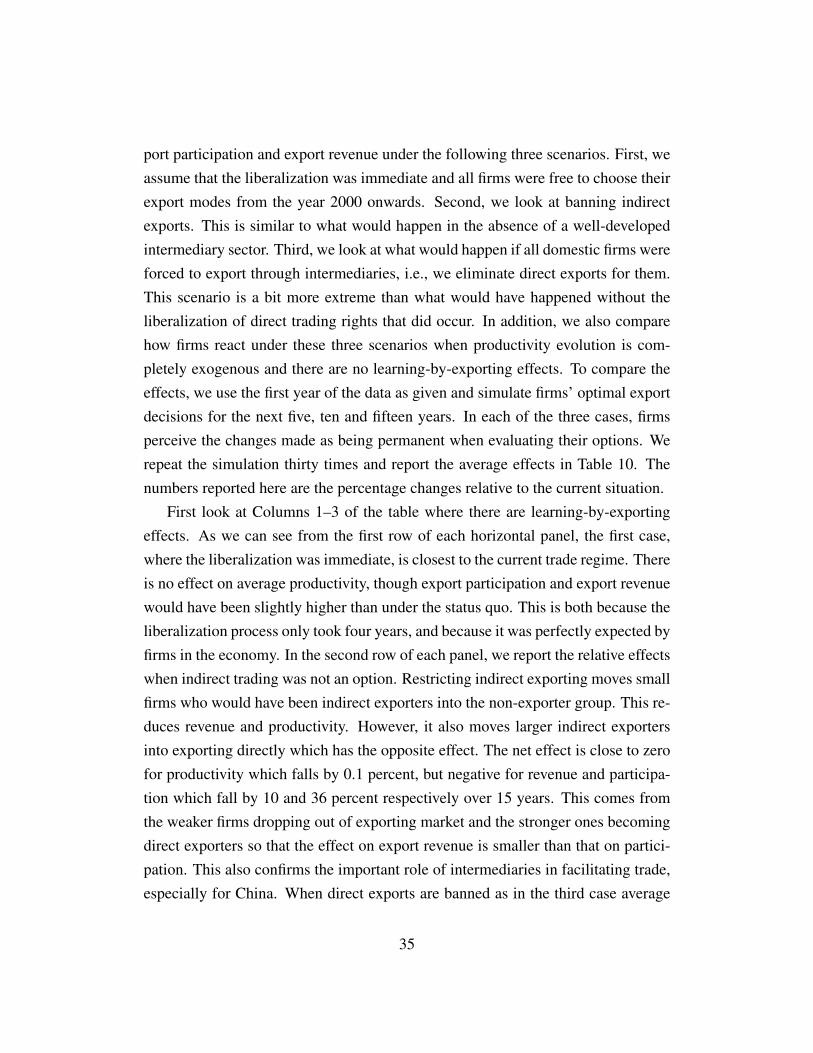
port participation and export revenue under the following three scenarios. First, weassume that the liberalization was immediate and all firms were free to choose theirexport modes from the year 2000 onwards. Second, we look at banning indirectexports. This is similar to what would happen in the absence of a well-developedintermediary sector. Third, we look at what would happen if all domestic firms wereforced to export through intermediaries, i.e., we eliminate direct exports for them.This scenario is a bit more extreme than what would have happened without theliberalization of direct trading rights that did occur. In addition, we also comparehow firms react under these three scenarios when productivity evolution is com-pletely exogenous and there are no learning-by-exporting effects. To compare theeffects, we use the first year of the data as given and simulate firms’ optimal exportdecisions for the next five, ten and fifteen years. In each of the three cases, firmsperceive the changes made as being permanent when evaluating their options. Werepeat the simulation thirty times and report the average effects in Table 10. Thenumbers reported here are the percentage changes relative to the current situation.

First look at Columns 1–3 of the table where there are learning-by-exportingeffects. As we can see from the first row of each horizontal panel, the first case,where the liberalization was immediate, is closest to the current trade regime. Thereis no effect on average productivity, though export participation and export revenuewould have been slightly higher than under the status quo. This is both because theliberalization process only took four years, and because it was perfectly expected byfirms in the economy. In the second row of each panel, we report the relative effectswhen indirect trading was not an option. Restricting indirect exporting moves smallfirms who would have been indirect exporters into the non-exporter group. This re-duces revenue and productivity. However, it also moves larger indirect exportersinto exporting directly which has the opposite effect. The net effect is close to zerofor productivity which falls by 0.1 percent, but negative for revenue and participa-tion which fall by 10 and 36 percent respectively over 15 years. This comes fromthe weaker firms dropping out of exporting market and the stronger ones becomingdirect exporters so that the effect on export revenue is smaller than that on partici-pation. This also confirms the important role of intermediaries in facilitating trade,especially for China. When direct exports are banned as in the third case average

35

productivity falls by 0.6 percent over the 15 years. Export participation and exportrevenue fall by 33 and 26 percent respectively.

Had there been no learning-by-exporting effects, shutting down the intermedi-ary sector would have decreased export revenue and participation by much more asthere are fewer benefits from exporting directly. In the same vein, without learning-by-exporting, the decreases in export revenue and participation from banning directexports would have been much smaller. This suggests that the effects via learning-by-exporting are critical. It is worth pointing out that this liberalization of directtrading rights was “revolutionary” (see footnote 2) given where China was comingfrom. In sum, the counterfacutals show that liberalizing direct trading rights wasimportant and exports would have been roughly a third lower had this not beendone. Our estimates have direct exporters have productivity growing at 2.5 percentcompared to 0.7 percent for indirect exporters, see Table 5. De Loecker (2013)shows that across all sectors, exporting and investing raises future productivity perannum from 1 to 8 percent and our estimates are of a similar magnitude.

6.2 Subsidies

A variety of trade policies have been used to encourage exports in developing coun-tries. The most commonly used tools include direct subsidies based on firms’ exportperformances, such as export revenue subsidies and duty-free access to importedinputs in export processing zones. Both of these tools have been used intensivelyby the Chinese government. This type of subsidy targets incumbent exporters andaffects exports on the intensive margin. At the same time, it increases exporters’survival rates and encourages entry just like a fall in variable costs. Other subsidies,like those to fixed and sunk costs, directly focus on reducing the cost of exportingand encourage net entry.

In this section, we simulate the effects of such subsidies. First, we simulate theeffect of a 5 and 10 percent subsidy on exports.46 We also simulate the effect ofa 25 and 50 percent reduction in fixed or sunk costs of exporting. In addition, we

46This can also be interpreted as the effect of a lower variable transportation cost or the develop-ment of transportation technologies or/and port facilities (as costs are of the iceberg variety) or VATrebates. This is because revenues are multiplicatively related to productivity and costs in our setting.

36

target the subsidies to different types of exporters. We take the first year of the dataand simulate trajectories of firm performance for future years. We compare all theresults to the case with no subsidies. In each of the three cases, firms perceive thepolicy to be permanent when evaluating their options.

Table 11 presents the results of this exercise ten years after the policy was in-troduced. We compare three measures of the effects of the subsidy: the increase inexport participation, export revenue and the ratio of increases in export revenue tothe subsidy costs. The last is the benefit to cost ratio and we focus on this.

First, we see that a 10 percent subsidy on exports increases the export partic-ipation rate by 4.7 percent and export revenue by 12.1 percent. The differencesuggests that this type of subsidy mainly operates through the intensive margin ofexports. In contrast, subsidizing the costs of exporting has a larger effect on in-creasing export participation than on export revenue. This is because subsidizingcosts operates through the entry-exit of firms into exporting. It is worth noting thatthe benefit-cost ratio of the export subsidy is higher when targeting direct exporters.This makes sense as they tend to be more productive. However, the benefit-cost ra-tio of cost subsidies is higher for indirect exporters as the costs of indirect exportingare lower.

7 Conclusion

Massive amounts of money has been allocated to “Aid for Trade” initiatives in de-veloping countries. The aim is to help developing countries overcome “trade-relatedconstraints” and to bring growth and reduce poverty. Yet, little is known aboutwhere the constraints are. Our paper has little to say about this and work in thisarea is sorely needed.

The policy conclusions we wish to highlight from our results are straightfor-ward. First, learning-by-exporting is important and is dramatically different acrossexport mode. Direct exporters seem to learn more about how to produce and whatto produce than indirect ones. For this reason alone, policies that encourage directexporting might be worth considering. We make the case that a hitherto less stud-ied policy, that of removing controls on direct exporting, had a significant effect on

37

promoting Chinese export growth. Of course, all the other policies that changedalso had an effect. In future work we hope to better understand the extent to whichChina’s domestic reforms, tariff reforms, and tariffs it faced, as well as its selectiveencouragement of sectors by fine-tuning VAT rebate levels, contributed to its exportgrowth.

References

Ahn, JaeBin, Amit K. Khandelwal, and Shang-Jin Wei, “The Role of Interme-diaries in Facilitating Trade,” Journal of International Economics, 2011, 84 (1),73–85.

Akerman, Anders, “A Theory on the Role of Wholesalers in International TradeBased on Economies of Scope,” Research Papers in Economics, 2010, 1.

Amiti, Mary and Jozef Konings, “Trade Liberalization, Intermediate Inputs, andProductivity: Evidence from Indonesia,” The American Economic Review, 2007,97 (5), 1611–1638.

Antràs, Pol and Arnaud Costinot, “Intermediated Trade,” The Quarterly Journal

of Economics, 2011, 126 (3), 1319–1374.

Arkolakis, Costas, “Market Penetration Costs and the New Consumers Margin inInternational Trade,” Journal of Political Economy, 2010, 118 (6), 1151–1199.

Aw, Bee Yan, Mark J. Roberts, and Daniel Yi Xu, “R&D Investment, Exporting,and Productivity Dynamics,” American Economic Review, 2011, 101 (4), 1312–44.

Bai, Xue and Kala Krishna, “Self Inflicted Wounds? China’s Restrictions onDirect Exporting,” 2014. Unpublished manuscript.

Baldwin, Richard and Paul Krugman, “Persistent Trade Effects of Large Ex-change Rate Shocks,” The Quarterly Journal of Economics, 1989, 104 (4), 635–654.

38

Bernard, Andrew B. and J. Bradford Jensen, “Exceptional Exporter Perfor-mance: Cause, Effect, or Both?,” Journal of International Economics, 1999, 47

(1), 1–25.

, Emily J. Blanchard, Ilke Van Beveren, and Hylke Y. Vandenbussche,“Carry-Along Trade,” NBER Working Paper Series, 2012, 18246.

, J. Bradford Jensen, Stephen J. Redding, and Peter K. Schott, “Firms inInternational Trade,” The Journal of Economic Perspectives, 2007, 21 (3), 105–130.

Biesebroeck, Johannes Van, “Exporting Raises Productivity in sub-SaharanAfrican Manufacturing Firms,” Journal of International Economics, 2005, 67

(2), 373–391.

Biglaiser, Gary, “Middlemen as Experts,” The RAND Journal of Economics, 1993,pp. 212–223.

Bloom, Nicholas, Mirko Draca, and John Van Reenen, “Trade Induced TechnicalChange? The Impact of Chinese Imports on Innovation, IT and Productivity,” The

Review of Economic Studies, 2016, 83 (1), 87–117.

Blum, Bernardo S., Sebastian Claro, and Ignatius Horstmann, “Intermediationand the Nature of Trade Costs: Theory and Evidence,” University of Toronto,

Mimeograph, 2009.

, , and , “Facts and figures on intermediated trade,” The American Economic

Review, 2010, 100 (2), 419–423.

Brandt, Loren, Johannes Van Biesebroeck, and Yifan Zhang, “Creative Ac-counting or Creative Destruction? Firm-level Productivity Growth in ChineseManufacturing,” Journal of Development Economic, 2012, 97 (2), 339–351.

Clerides, Sofronis K., Saul Lach, and James R. Tybout, “Is Learning by Ex-porting Important? Micro-dynamic Evidence from Colombia, Mexico, and Mo-rocco,” The Quarterly Journal of Economics, 1998, 113 (3), 903–947.

39

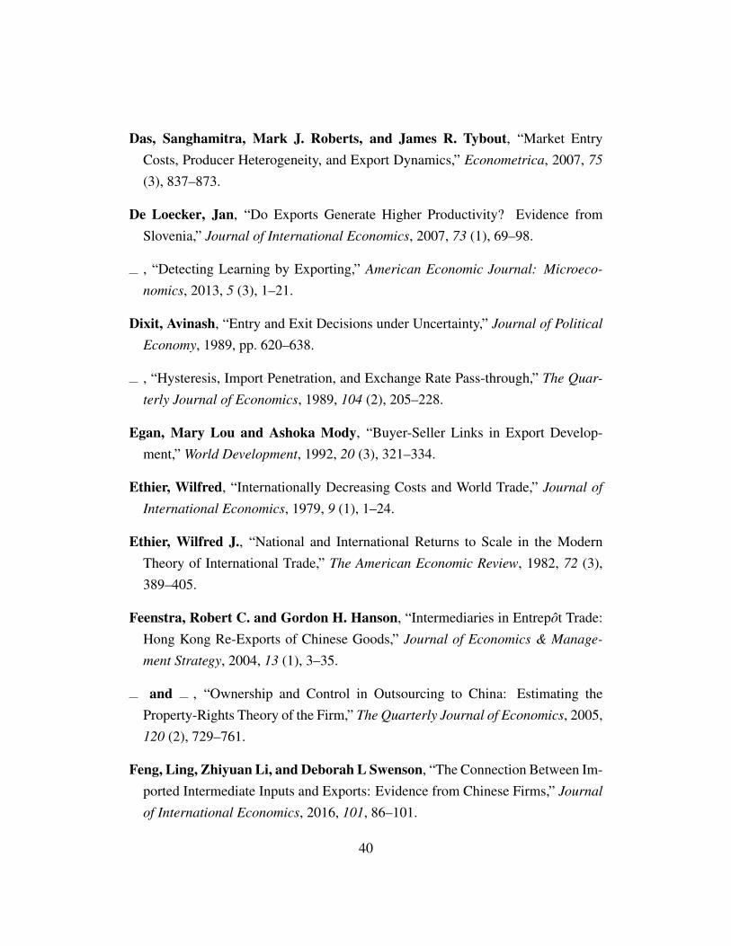
Das, Sanghamitra, Mark J. Roberts, and James R. Tybout, “Market EntryCosts, Producer Heterogeneity, and Export Dynamics,” Econometrica, 2007, 75

(3), 837–873.

De Loecker, Jan, “Do Exports Generate Higher Productivity? Evidence fromSlovenia,” Journal of International Economics, 2007, 73 (1), 69–98.

, “Detecting Learning by Exporting,” American Economic Journal: Microeco-

nomics, 2013, 5 (3), 1–21.

Dixit, Avinash, “Entry and Exit Decisions under Uncertainty,” Journal of Political

Economy, 1989, pp. 620–638.

, “Hysteresis, Import Penetration, and Exchange Rate Pass-through,” The Quar-

terly Journal of Economics, 1989, 104 (2), 205–228.

Egan, Mary Lou and Ashoka Mody, “Buyer-Seller Links in Export Develop-ment,” World Development, 1992, 20 (3), 321–334.

Ethier, Wilfred, “Internationally Decreasing Costs and World Trade,” Journal of

International Economics, 1979, 9 (1), 1–24.

Ethier, Wilfred J., “National and International Returns to Scale in the ModernTheory of International Trade,” The American Economic Review, 1982, 72 (3),389–405.

Feenstra, Robert C. and Gordon H. Hanson, “Intermediaries in Entrepot Trade:Hong Kong Re-Exports of Chinese Goods,” Journal of Economics & Manage-

ment Strategy, 2004, 13 (1), 3–35.

and , “Ownership and Control in Outsourcing to China: Estimating theProperty-Rights Theory of the Firm,” The Quarterly Journal of Economics, 2005,120 (2), 729–761.

Feng, Ling, Zhiyuan Li, and Deborah L Swenson, “The Connection Between Im-ported Intermediate Inputs and Exports: Evidence from Chinese Firms,” Journal

of International Economics, 2016, 101, 86–101.

40

Goldberg, Pinelopi K., Amit K. Khandelwal, Nina Pavcnik, and PetiaTopalova, “Imported Intermediate Inputs and Domestic Product Growth: Evi-dence from India,” The Quarterly Journal of Economics, 2010, 125 (4), 1727–1767.

Handley, Kyle and Nuno Limão, “Policy Uncertainty, Trade and Welfare: Theoryand Evidence for China and the US,” NBER Working Paper Series, 2013, 19376.

Head, Keith, Ran Jing, and Deborah L Swenson, “From Beijing to Bentonville:Do Multinational Retailers Link Markets?,” Journal of Development Economics,2014, 110, 79–92.

Kasahara, Hiroyuki and Beverly Lapham, “Productivity and the Decision to Im-port and Export: Theory and Evidence,” Journal of International Economics,2013, 89 (2), 297–316.

and Joel Rodrigue, “Does the Use of Imported Intermediates Increase Produc-tivity? Plant-level Evidence,” Journal of Development Economics, 2008, 87 (1),106–118.

Krishna, Kala and Ling Hui Tan, Rags and Riches: Implementing Apparel Quo-

tas under the Multi-Fibre Arrangement, University of Michigan Press, 1998.

Levinsohn, James and Amil Petrin, “Estimating Production Functions Using In-puts to Control for Unobservables,” The Review of Economic Studies, 2003, 70

(2), 317–341.

Melitz, Marc J., “The Impact of Trade on Intra-Industry Reallocations and Aggre-gate Industry Productivity,” Econometrica, 2003, 71 (6), 1695–1725.

Pierce, Justin R. and Peter K. Schott, “The Surprisingly Swift Decline of USManufacturing Employment,” NBER Working Paper Series, 2012, 18655.

Roberts, Mark J. and James R. Tybout, “The Decision to Export in Colombia:An Empirical Model of Entry with Sunk Costs,” The American Economic Review,1997, 87 (4), 545–564.

41

Rossman, Marlene L, “Export Trading Company Legislation: US Response toJapanese Foreign Market Penetration,” Journal of Small Business Management,1984, 22 (4), 62–64.

Rubinstein, Ariel and Asher Wolinsky, “Middlemen,” The Quarterly Journal of

Economics, 1987, 102 (3), 581–593.

Zhang, Hongsong, “Static and Dynamic Gains from Importing Intermediate In-puts: Theory and Evidence,” The Pennsylvania State University, Mimeograph,2013.

42

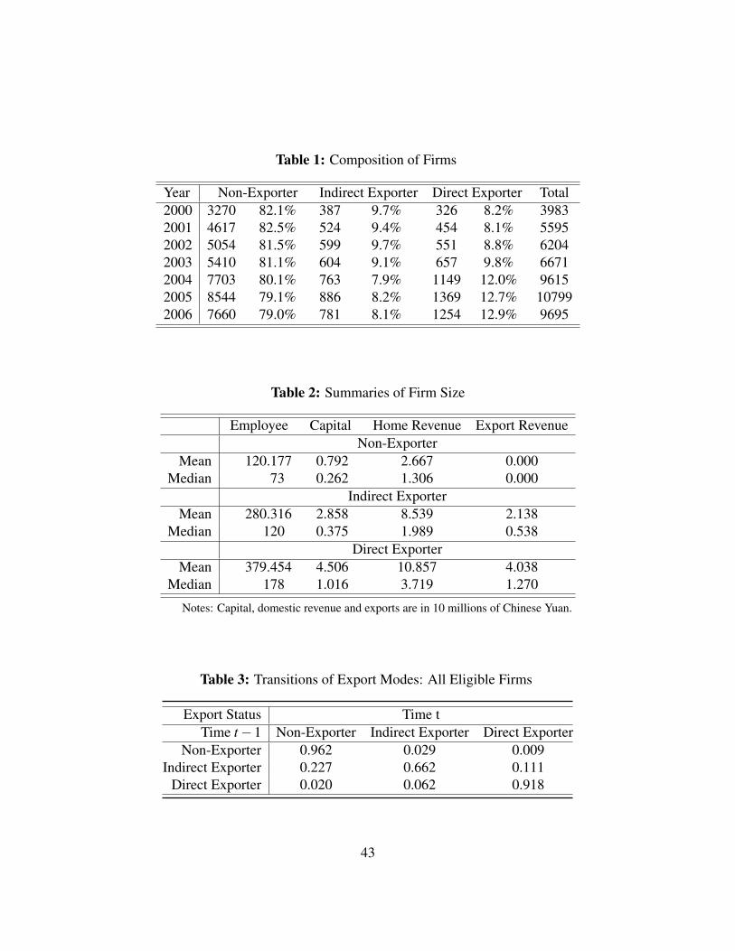
Table 1: Composition of Firms

Year Non-Exporter Indirect Exporter Direct Exporter Total2000 3270 82.1% 387 9.7% 326 8.2% 39832001 4617 82.5% 524 9.4% 454 8.1% 55952002 5054 81.5% 599 9.7% 551 8.8% 62042003 5410 81.1% 604 9.1% 657 9.8% 66712004 7703 80.1% 763 7.9% 1149 12.0% 96152005 8544 79.1% 886 8.2% 1369 12.7% 107992006 7660 79.0% 781 8.1% 1254 12.9% 9695

Table 2: Summaries of Firm Size

Employee Capital Home Revenue Export RevenueNon-Exporter

Mean 120.177 0.792 2.667 0.000Median 73 0.262 1.306 0.000

Indirect ExporterMean 280.316 2.858 8.539 2.138

Median 120 0.375 1.989 0.538Direct Exporter

Mean 379.454 4.506 10.857 4.038Median 178 1.016 3.719 1.270

Notes: Capital, domestic revenue and exports are in 10 millions of Chinese Yuan.

Table 3: Transitions of Export Modes: All Eligible Firms

Export Status Time tTime t−1 Non-Exporter Indirect Exporter Direct Exporter

Non-Exporter 0.962 0.029 0.009Indirect Exporter 0.227 0.662 0.111

Direct Exporter 0.020 0.062 0.918

43

Table 4: Costs of Exporting

Export Status Time tTime t−1 Non-Exporter Indirect Exporter Direct Exporter

Non-Exporter 0 γHISit γHDS

it

Indirect Exporter 0 γ IFit γ IDS

it

Direct Exporter 0 γDISit γDF

it

Indirect Exporter at t − 1

StopExporting

Continue IndirectExporting

Start DirectExporting

domestic profit

− no extra cost

+ δEV H

domestic profit

+ foreign IE profit

− fixed cost γIF

+ δEV I

domestic profit

+ foreign DE profit

− sunk cost γIDS

+ δEV D

Figure 1. Example of a Firm’s Dynamic Decisions

44

Table 5: Demand Elasticities, Marginal Cost, and Productivity Evolution

Rubber Chemical Machinery FurnitureParameters & Plastic & Eqpt

Domestic Elasticity σH 4.679*** 5.506*** 5.401*** 5.539***(0.003) (0.002) (0.002) (0.006)

Foreign Elasticity σX 4.405*** 3.530*** 4.581*** 7.059***(0.008) (0.009) (0.004) (0.010)

Capital βk -0.070*** -0.057*** -0.057*** -0.043***(0.002) (0.001) (0.001) (0.002)

Constant α0 0.542*** 0.515*** 0.323*** -0.273***(0.032) (0.017) (0.014) (0.093)

ωωω t−1 α1 0.303*** 0.188*** 0.549*** 1.730***(0.068) (0.041) (0.034) (0.172)

ωωω2t−1 α2 0.264*** 0.398*** 0.206*** -0.488***

(0.050) (0.034) (0.027) (0.104)ωωω3

t−1 α3 -0.028** -0.061*** -0.032*** 0.096***(0.012) (0.008) (0.007) (0.020)

Indirect Exportt−1 α4 0.007*** 0.004*** 0.006*** -0.001(0.002) (0.001) (0.001) (0.002)

Direct Exportt−1 α5 0.025*** 0.017*** 0.019*** 0.014***(0.002) (0.001) (0.001) (0.002)

ΨH 2.392 2.161 1.799 0.072σω 0.129 0.115 0.116 0.104

∗∗∗,∗∗ and ∗ indicate significance at the 1%, 5% and 10% levels, respectively.

45

0.2

.4.6

.81

Den

sity

.14 .5 1 1.5 2 2.62Productivity

Non-ExportersIndirect ExportersDirect Exporters

kernel = epanechnikov, bandwidth = 0.3200

Kernel Density Estimates of Productivity by Export Modes - ISIC 25

Figure 2. Productivity Distributions by Export Modes

46

0.2

.4.6

.81

Den

sity

.29 .5 1 1.5 2 2.51Productivity

Non-Exporters 2001Non-Exporters 2006

kernel = epanechnikov, bandwidth = 0.3200

Productivity Distribution 2001 v.s. 2006: Non-Exporters0

.2.4

.6.8

1D

ensi

ty

.29 .5 1 1.5 2 2.51Productivity

Indirect Exporters 2001Indirect Exporters 2006

kernel = epanechnikov, bandwidth = 0.3200

Productivity Distribution 2001 v.s. 2006: Indirect Exporters

0.2

.4.6

.81

Den

sity

.29 .5 1 1.5 2 2.51Productivity

Direct Exporters 2001Direct Exporters 2006

kernel = epanechnikov, bandwidth = 0.3200

Productivity Distribution 2001 v.s. 2006: Direct Exporters

Figure 3. Evolution of Productivity Distributions: 2001 & 2006

47

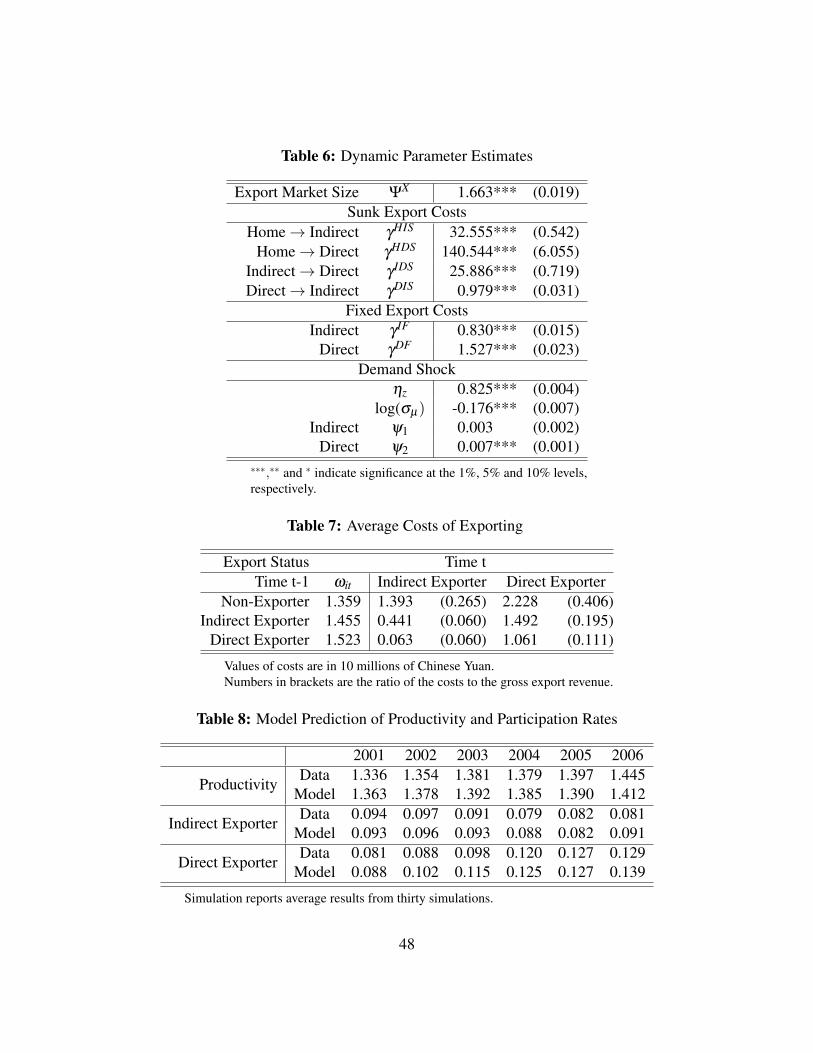
Table 6: Dynamic Parameter Estimates

Export Market Size ΨX 1.663*** (0.019)Sunk Export Costs

Home→ Indirect γHIS 32.555*** (0.542)Home→ Direct γHDS 140.544*** (6.055)

Indirect→ Direct γ IDS 25.886*** (0.719)Direct→ Indirect γDIS 0.979*** (0.031)

Fixed Export CostsIndirect γ IF 0.830*** (0.015)

Direct γDF 1.527*** (0.023)Demand Shock

ηz 0.825*** (0.004)log(σµ) -0.176*** (0.007)

Indirect ψ1 0.003*** (0.002)Direct ψ2 0.007*** (0.001)

∗∗∗,∗∗ and ∗ indicate significance at the 1%, 5% and 10% levels,respectively.

Table 7: Average Costs of Exporting

Export Status Time tTime t-1 ωit Indirect Exporter Direct Exporter

Non-Exporter 1.359 1.393 (0.265) 2.228 (0.406)Indirect Exporter 1.455 0.441 (0.060) 1.492 (0.195)

Direct Exporter 1.523 0.063 (0.060) 1.061 (0.111)

Values of costs are in 10 millions of Chinese Yuan.Numbers in brackets are the ratio of the costs to the gross export revenue.

Table 8: Model Prediction of Productivity and Participation Rates

2001 2002 2003 2004 2005 2006

ProductivityData 1.336 1.354 1.381 1.379 1.397 1.445

Model 1.363 1.378 1.392 1.385 1.390 1.412

Indirect ExporterData 0.094 0.097 0.091 0.079 0.082 0.081

Model 0.093 0.096 0.093 0.088 0.082 0.091

Direct ExporterData 0.081 0.088 0.098 0.120 0.127 0.129

Model 0.088 0.102 0.115 0.125 0.127 0.139

Simulation reports average results from thirty simulations.

48

Table 9: Model Prediction of Transition Rates

Export Status Time tTime t−1 Non-Exporter Indirect Exporter Direct Exporter

Non-ExporterData 0.962 0.029 0.009

Model 0.942 0.038 0.020

Indirect ExporterData 0.227 0.662 0.111

Model 0.247 0.616 0.137

Direct ExporterData 0.020 0.062 0.918

Model 0.065 0.066 0.869

Simulation reports average results from thirty simulations.

Table 10: Firm Response Under Different Liberalization Scenarios

Policy Regimes Learning No LearningYears since 2000 5 10 15 5 10 15

Average ProductivityNo Restriction 0.0 0.0 0.0 0.0 0.0 0.0No Intermediary 0.0 -0.1 -0.1 0.0 0.0 0.0No Liberalization -0.1 -0.4 -0.6 0.0 0.0 0.0

Export ParticipationNo Restriction 0.3 0.0 0.0 0.1 0.0 0.0No Intermediary -34.6 -35.2 -35.8 -51.0 -53.7 -53.3No Liberalization -21.3 -30.6 -33.4 -5.8 -6.8 -6.7

Export RevenueNo Restriction 0.2 0.1 0.0 0.0 0.0 0.0No Intermediary -21.1 -17.6 -9.7 -23.1 -23.3 -21.0No Liberalization -13.5 -21.6 -25.7 -3.4 -3.6 -3.7

Numbers in the table represent the percentage change compared to the currentscenario.

49

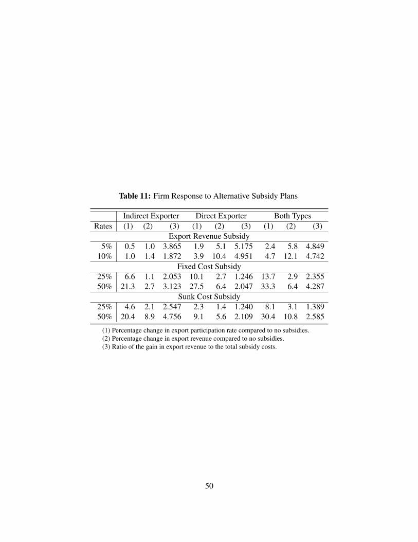
Table 11: Firm Response to Alternative Subsidy Plans

Indirect Exporter Direct Exporter Both TypesRates (1) (2) (3) (1) (2) (3) (1) (2) (3)

Export Revenue Subsidy5% 0.5 1.0 3.865 1.9 5.1 5.175 2.4 5.8 4.849

10% 1.0 1.4 1.872 3.9 10.4 4.951 4.7 12.1 4.742Fixed Cost Subsidy

25% 6.6 1.1 2.053 10.1 2.7 1.246 13.7 2.9 2.35550% 21.3 2.7 3.123 27.5 6.4 2.047 33.3 6.4 4.287

Sunk Cost Subsidy25% 4.6 2.1 2.547 2.3 1.4 1.240 8.1 3.1 1.38950% 20.4 8.9 4.756 9.1 5.6 2.109 30.4 10.8 2.585

(1) Percentage change in export participation rate compared to no subsidies.(2) Percentage change in export revenue compared to no subsidies.(3) Ratio of the gain in export revenue to the total subsidy costs.

50

Appendix

This appendix provides supplemental information on details of second-stage estimation, the re-strictions on direct trading rights in China, the data sets used in this paper and robustness checksfor the model.

A Details on Second-Stage Estimation

Following Das et al. (2007) and Aw et al. (2011), we estimate the model using a two-stage ap-proach. In the first stage of the estimation, we recovered the following parameters using data ontotal variable cost, domestic revenue, export revenue, capital size, intermediate materials, exportmodes, year, industry and location: the elasticities of substitution in the two markets (σHand σX ),the home market size intercept (ΦH

t ), the marginal cost parameter (βk), the productivity evolutionfunction (g(ωit−1,dit−1)), and the variance of transient productivity shocks (σ2

ξ).

In the second stage, based on the estimates from the first stage, we construct and estimatethe dynamic discrete choice problem to obtain the parameters on the foreign market size (ΦX

t ),demand shock evolution (ηz, σµ , ψ1, ψ2) and the distribution of both sunk and fixed costs (Gγ ).In the following sections, we provide details on the construction and estimation of the dynamicdiscrete choice problem.

A.1 Dynamic Optimization Problem

At the beginning of each period, firm i observes the current state, sit =(ωit ,zit ,dddit−1,Φ

Ht ,Φ

Xt ,wwwit

)which includes its current productivity and demand shocks (ωit ,zit) and its past decision regardingwhich markets to serve and its export mode (dddit−1), the price indices in the markets (ΦH

t ,ΦXt ) as

well as the firm-time specific factor prices it faces, wwwit . We will suppress wwwit ,ΦHt ,Φ

Xt , as these are

not chosen by the firm and call the state space sit = (ωit ,zit ,dddit−1) from now on. It then draws itsfixed and sunk costs for all the relevant options open to it and then chooses whether to sell onlydomestically, export indirectly, or export directly.47 We allow the distributions of the costs, bothfixed and sunk, of exporting to differ depending on the firm’s past and current exporting status andmode. All this is summarized in Table 4.

Knowing sit , the firm’s value function in year t, before it observes its fixed and sunk costs, canbe written as the integral over these costs when the firm chooses the best option today (it maximizes

47Firms that don’t have direct trading rights can only choose whether to stay domestic or export indirectly, and theirexport dynamic problems are adjusted accordingly.

51

over dddit = (dHit ,d

Iit ,d

Dit )) and optimizes from the next period onwards:

V (sit) =∫

maxdddit

[u(dddit ,sit |γγγ it)+δEtV (sit+1 |dddit )]dGγγγ , (A.1)

where u(dddit ,sit |γγγ it) is the current period payoff and depends on the choice of export status andmode, dddit , the state sit (which includes last period’s demand and productivity draws as well asexport status and mode of exporting) and the relevant sunk and fixed cost shocks drawn, γγγ it :

u(dddit ,sit |γγγ it) = πHit +dI

it

[π

XIit −

(dH

it−1γHISit +dI

it−1γIFit +dD

it−1γDISit

)](A.2)

+ dDit

[π

XDit −

(dH

it−1γHDSit +dI

it−1γIDSit +dD

it−1γDFit

)].

where per-period variable profits (before the sunk and fixed costs) in different markets are givenby

πHit =

1σH rH

it =1

σH

[σH

σH−1c(wwwit)

eωit

]1−σHY H

t(PH

t)1−σX ezit

πXIit =

1σX rXI

it =1

σX λ−σX

[σX

σX −1c(wwwit)

eωit

]1−σXY X

t(PX

t)1−σX ezit (A.3)

πXDit =

1σX rXD

it =1

σX

[σX

σX −1c(wwwit)

eωit

]1−σXY X

t(PX

t)1−σX ezit

The continuation value is

EtV (sit+1 |dddit ) =∫

z′

∫ω′ V(

s′)

dF(

ω′ |ωit ,dddit

)dF(

z′ |zit ,dddit

), (A.4)

where dF(

ω′ |ωit ,dddit

)and dF

(z′ |zit ,dddit

)are the evolutions of productivity and demand shock

as defined in equations (17) and (18).

A.2 Choice Probability and Value Function

For any state vector, denote the choice-specific continuation value from choosing dmit = 0,1, as

EtV mit+1 = EtV (sit+1 |dm

it = 1) , m = H, I,D. Firms’ export decisions depend on the difference inthe pair-wise marginal benefits between any two options and the associated sunk/fixed costs. Themarginal benefits of being an indirect exporter versus being a non-exporter, the marginal benefitsof being a direct exporter versus not exporting, and the marginal benefits of being a direct exporter

52

versus being an indirect one, are defined in equations (A.5), respectively.48

∆IHit = πXIit +δ

(EtV I

it+1−EtV Hit+1)

∆DHit = πXDit +δ

(EtV D

it+1−EtV Hit+1)

(A.5)

∆DIit = πXDit −π

XIit +δ

(EtV D

it+1−EtV Iit+1)

Given the distribution of costs, these marginal benefits and export modes in the last periodpin down the probability of switching export modes or not doing so. Specifically, for any set ofrealized export costs, γγγ t =

(γHDS

it ,γ IDSit ,γDF

it ,γHISit ,γDIS

it ,γ IFit), the following show the differences in

life-time payoff between any two different current export modes that are unconditional on previousexport mode.

yDHit = ∆DHit− I (dit−1 = H)γ

HDSit − I (dit−1 = I)γ

IDSit − I (dit−1 = D)γ

DFit

yIHit = ∆IHit− I (dit−1 = H)γ

HISit − I (dit−1 = D)γ

DISit − I (dit−1 = I)γ

IFit (A.6)

yDIit = ∆DIit− [I (dit−1 = H)γ

HDSit + I (dit−1 = I)γ

IDSit + I (dit−1 = D)γ

DFit

− I (dit−1 = H)γHISit − I (dit−1 = D)γ

DISit − I (dit−1 = I)γ

IFit ]

Thus, the unconditional choice probability between any two different export modes are givenas

P(yDHit > 0) = P

[I (dit−1 = H)γ

HDSit + I (dit−1 = I)γ

IDSit + I (dit−1 = D)γ

DFit ≤ ∆DHit

]P(yIH

it > 0) = P[I (dit−1 = H)γ

HISit + I (dit−1 = D)γ

DISit + I (dit−1 = I)γ

IFit ≤ ∆IHit

]P(yDI

it > 0)

= P[I (dit−1 = H)γ

HDSit + I (dit−1 = I)γ

IDSit + I (dit−1 = D)γ

DFit

](A.7)[

− I (dit−1 = H)γHISit − I (dit−1 = D)γ

DISit − I (dit−1 = I)γ

IFit ≤ ∆DIit

]Hence, conditioning on the previous export mode, the probability of firm i at time t can be

written as the following. This corresponds to the empirical transition matrix in Table 3. For a

48∆HIit , ∆HDit , and ∆IDit could be similarly defined but simple calculations show that they are merely the negativeof ∆IHit , ∆DHit , and ∆DIit .

53

previous non-exporter, the probability to stay as non-exporter, to become an indirect exporter andto become a direct exporter are given as follows respectively.

PHHit = P(yIH

it ≤ 0 & yDHit ≤ 0) = P

[γ

HISit ≥ ∆IHit

]·P[γ

HDSit ≥ ∆DHit

]PHI

it = P(yIHit > 0 & yDI

it ≤ 0) = P[γ

HISit < min

∆IHit ,γ

HDSit −∆DIit

](A.8)

PHDit = P(yDH

it > 0 & yDIit > 0) = P

[γ

HDSit < min

∆DHit ,γ

HISit +∆DIit

]Thus, after rewriting equation (A.1), the value function for a previous non-exporter updates ac-cording to the following formula.

V Hit = π

Hit + PHH

it ·[δEtV H

it+1]

+ PHIit ·

[π

XIit −E

(γ

HISit

∣∣∣γHISit < min

∆IHit ,γ

HDSit −∆DIit

)+δEtV I

it+1

](A.9)

+ PHDit ·

[π

XDit −E

(γ

HDSit

∣∣∣γHDSit < min

∆DHit ,γ

HISit +∆DIit

)+δEtV D

it+1

]Similarly, given his previous export mode, a previous indirect exporter optimizes according to thefollowing choice probabilities

PIHit = P(yIH

it ≤ 0 & yDHit ≤ 0) = P

[γ

IFit ≤ ∆IHit

]·P[γ

IDSit ≤ ∆DHit

]PII

it = P(yIHit > 0 & yDI

it ≤ 0) = P[γ

IFit < min

∆IHit ,γ

IDSit −∆DIit

](A.10)

PIDit = P(yDH

it > 0 & yDIit > 0) = P

[γ

IDSit < min

∆DHit ,γ

IFit +∆DIit

],

and value function updating rule,

V Iit = π

Hit + PIH

it ·[δEtV H

it+1]

+ PIIit ·[π

XIit −E

(γ

IFit

∣∣∣γ IFit < min

∆IHit ,γ

IDSit −∆DIit

)+δEtV I

it+1

](A.11)

+ PIDit ·[π

XDit −E

(γ

IDSit

∣∣∣γ IDSit < min

∆DHit ,γ

IFit +∆DIit

)+δEtV D

it+1

].

For a previous direct exporter, we can write the same choice probabilities and value function

54

iteration.

PDHit = P(yIH

it ≤ 0 & yDHit ≤ 0) = P

[γ

DISit > ∆IHit

]·P[γ

DFit > ∆DHit

]PDI

it = P(yIHit > 0 & yDI

it ≤ 0) = P[γ

DISit < min

∆IHit ,γ

DFit −∆DIit

](A.12)

PDDit = P(yDH

it > 0 & yDIit > 0) = P

[γ

DFit < min

∆DH,γDIS +∆DIit

]V D

it = πHit + PDH

it ·[δEtV H

it+1]

+ PDIit ·

[π

XIit −E

(γ

DISit

∣∣∣γDISit < min

∆IHit ,γ

DFit −∆DIit

)+δEtV I

it+1

](A.13)

+ PDDit ·

[π

XDit −E

(γ

DFit

∣∣∣γDFit < min

∆DHit ,γ

DISit +∆DIit

)+δEtV D

it+1

]A.3 Dynamic Estimation

We estimate the dynamic parameters by maximizing the likelihood function for the observed par-ticipation and modes of exporting along with the observed export revenue. The level of each firm’sexport revenue provides information on the demand shocks once we know the firm’s industry andlocation, productivity, capital stock (a cost shifter), market size. This information is observableconditioning on exporting. Hence the demand shock distribution is censored so that we do notobserve the demand shocks of non-exporters. We follow Das et al. (2007) and Aw et al. (2011)to infer the unconditional distribution for the demand shocks based on the conditional distribu-tion. Based on the first-stage parameter estimates and productivity estimates, we can write firm i’scontribution to the likelihood function as

P(dddi,rXm

i |ωi,ki,Φ)= P

(dddi∣∣ωi,ki,Φ,z+i

)f(z+i)

(A.14)

where f (·) is the marginal distribution of z and z+i is the series of foreign market demand shocksin the years when firm i exports. In the evaluation of the likelihood function, we followed Das etal. (2007) and Aw et al. (2011) to construct the density f (·) and simulate the unobserved exportmarket shocks.

We solve each firm’s dynamic optimization problem using the following algorithm:

1. Begin with an initial guess of parameters (ΦX0t ,η0

z ,σ0µ ,ψ

01 ,ψ

02 ,G

γγγ0)

2. Given the parameters, backout and simulate z shocks based on observed export values, basedthe export profit functions (A.3) and guessed parameters (ΦX0

t ,η0z ,σ

0µ ,ψ

01 ,ψ

02 ). Then cal-

55

culate F(

z′ |z,ddd

)based on equations (18). F

(ω′ |ω,ddd

)can be calculated outside the loop

based on parameters from the first-stage estimation.

3. Iterate on the following inner loop to find fixed points of value functions.

(a) Start with a set of initial guess of value functions V m0(s),m = H, I,D, where s =(ω,z,ddd−1,Φ

H ,ΦX ,www)

(b) According to equations (A.1) and (A.4), calculate the continuation values for every ex-port mode EV m0 =

∫z′∫

ω′ V m0

(s′)

dF(

ω′ |ω,dm

it = 1)

dF(

z′ |z,dm

it = 1)

, where m =

H, I,D.

(c) Update value functions for every export mode according to equations (A.9), (A.11) and(A.13). The choice probabilities are calculated based on equations (A.8), (A.10) and(A.12). For example, for a previous non-exporter:

V H1(s) = πH + PHH ·

[δEV H0]

+ PHI ·[π

XI−E(

γHIS∣∣∣γHIS < min

∆IH,γHDS−∆DI

)+δEV I0

]+ PHD ·

[π

XD−E(

γHDS

∣∣∣γHDS < min

∆DH,γHIS +∆DI)

+δEV D0]

(d) Iterate step (a)-(c) until |V mn+1−V mn|< ε for every m = H, I,D.

4. Evaluate the likelihood function for every observation.

We followed the methods in Aw et al. (2011) to discretize the state space. For data points thatare not on the grid we use the same procedure as in Aw et al. (2011).

B Restriction on Direct Trading Rights

China began to open up its economy in the late 1970s. Before a series of trade policy reforms,Chinese trade was dominated by a few Foreign Trade Corporations (FTC) with monopoly tradingrights. By the end of 1978, there were less than 20 such FTCs and around 100 subsidiaries of theseFTCs controlled by the central government. The Foreign Trade Law adopted in 1994 formalizedthe so called “approval system” of foreign trade rights. Restrictions on direct trading rights appliedonly to domestically-owned firms while foreign-invested firms automatically had direct tradingrights. In 1998, the State Council approved the issuing of direct trading rights to private domesticentities whose registered capital, revenue, net assets, and exports exceeded certain threshold lev-

56

els.49 The thresholds were reduced and the restrictions eliminated over the period 2000 to 2004 aspart of the accession agreement for joining the WTO. The details of the rules governing the abilityto trade directly in the period 1999-2004 are laid out in Table A.1 below. Before 2001, privatedomestic firms faced multiple threshold requirements as explained above, but after 2001, they onlyneeded to qualify in terms of their registered capital. Until 2001, they needed to formally apply forapproval while after 2001, approval was automatically given.

Before 2001, State or Public-owned enterprises and firms in Special Economic Zones facedthresholds only on registered capital. In 2001, the requirements were made homogeneous acrossall types of firms, other than those in SEZs, whose requirements were less restrictive. In the middleof 2001 and then again later on, this common threshold for registered capital was lowered. By July2004, the Chinese government removed all restrictions on direct trading rights.

Firms in Pudong were only treated differently from other firms (of the same type) in that theregistered capital requirement was reduced for them in 2002, a year and a half before it was reducedfor other firms.

C Data Matching

This section provides detailed information on the quality of the match between the firm-level sur-vey data and the transaction-level customs data used in this paper. The difficulty of matchingthese two data sets lies in the fact that the firm identification codes used in the two data sets arecompletely different. Thus we matched the data on the basis of firm name, region code, address,legal representative, and other information that identifies the firm. Firms were matched in multipledimensions and a score was assigned which increased with the dimensions in which the recordsmatched. All matches above a cutoff score were accepted. Below the cutoff, each case was manu-ally examined.

Table A.2 and Table A.3 provide information on the percentage of the total number of exportersand total value of exports matched based on the customs data. In each of these two tables, the firsthorizontal panel shows the number of exporters or the value of exports accounted for by interme-diaries. Below this is their share of the total. As in Ahn et al. (2011), we identify intermediaries inthe customs data based on their names. For example, in 2004, intermediaries account for 18.1 per-cent of the total number of exporters. This means that in 2004, 81.9 percent of the total exporters

49Registered capital is also known as the authorized capital. It is the maximum value of securities that a company canlegally issue. This number is specified in the memorandum of association (or articles of incorporation in the US) whena company is incorporated. It is also called authorized stock, nominal capital, nominal share capital. Registered capitalmay be divided into (1) issued capital: par value of the shares actually issued; (2) paid up capital: money receivedfrom the shareholders in exchange for shares; (3) uncalled capital: money remaining unpaid by the shareholders forthe shares they have bought. By law, in China, a firm’s paid up capital should be equal to its registered capital.

57

are producing exporters, matched, unmatched, and unsurveyed.The second horizontal panel of these two tables shows the number of exporters or the value of

exports that have been matched. Below this is their share in the total. From the second panel ofA.2, we can see that 46.8 percent of the total number of exporters observed in the customs data arematched with the firm-level data in 2004.

The third horizontal panel then shows the share of exporters that are unmatched or unsurveyedor the exports that are accounted for by these exporters. Below this is their share in the total. Wecan see that we have matched about 50 percent of the data in terms of the number of producingexporters and about 80 percent in terms of export values that belong to these producing exporters.

We can better understand the third panel by looking at the Census data. Based on the Censusdata from 2004, 39 percent of the producers who export are below the Census threshold and accountfor 2 percent of the total export value.

D Inferred Export Modes

Recall that we infer export modes as firms are not directly asked about their mode of export.Hence, mis-reporting in the survey and errors or mismatches in the process of merging the twodata sets could create errors in our classification.50 For example, some firms may say they didnot export because they did not realize the intermediary they sold to was exporting their goods.Consequently, we could have mis-classified indirect exporters as non-exporters. This is unlikely asexporting intermediaries have names that clearly differentiate them from domestic ones as madeclear in Ahn et al. (2011). In any case, this mis-classification would work in our favor as it wouldreduce growth of demand shocks and productivity of exporters relative to non-exporters.

More importantly, we could be mis-classifying firms because our match of the survey to thecustoms data is poor. If this were the case, there would be many firms who are actually in bothdata sets but whom we cannot match and so end up being mis classified as indirect exporters. Weexamine the robustness of our definition of indirect and direct exporters by comparing the evermatched and never matched indirect exporters. Ever matched indirect exporters are the inferredindirect exporters who have been matched at least once with the customs data. Once these exportersare matched, we know their identification number in the customs data and are able to track theirexport modes over time. They are the ones who we can see switching between indirect and directexport modes. Never matched indirect exporters are the ones who could be wrongly labeled asindirect exporters, just because they are not matched with the customs data in any sample year.Could these never matched indirect exporters actually be unmatched direct exporters? This is whatwe want to check.

50Evidence on match quality is discussed in the second section C of the Appendix.

58

We estimate the predicted probability of each firm-time observation being (observed as) a directexporter using a probit model.

eit = 111 [βeit−1 +ηDomt +Xitφ +νit > 0]

eit equals one if exporter i is directly exporting (or being matched with the customs data) at timet. Domt is a set of ownership, industry and time dummies and Xit includes other firm-time levelcovariates such as log capital, log employee, eligibility of direct trading rights, log revenue, previ-ous export modes, etc. Figure A.1 compares the distribution of the predicted probability of beinga direct exporter for firms we classify as direct exporters, ever matched indirect exporters, nevermatched indirect exporters and non-exporters.

From these histograms we can see that the distribution of the never matched looks like it liesbetween that of non-exporters and ever matched indirect exporters, which makes them closer toindirect exporters than to direct exporters. This gives us some confidence that we are not mis-classifying firms. We further examine the robustness of our model to alternative definitions ofexport modes in the next section.

E Robustness Checks

In this section, we provide robustness checks of our benchmark model in terms of productivityevolution, especially learning effects from different export modes. Specifically, we re-estimatethe first stage of our model using alternative productivity measures, alternative definitions of ex-port modes, different evolution processes of productivity. We also control for types of products,destination countries and other firm decisions.

E.1 Other Productivity Measures

All previous robustness checks are based on the model assumptions that consumers have CESpreferences while firms compete monopolistically and produces at constant marginal cost. We alsoused time, industry, location dummies and log capital stock to capture time-varying and firm-timevarying cost shifters. These productivity measures are identified within the model from firms’ do-mestic revenue function. Table A.4 shows the productivity evolution using alternative productivitymeasures. In column 2, we replicate the Tornqvist index productivity measure in Brandt et al.(2012) and show the evolution of productivity allowing for learning-by-exporting. In Columns 3and 4, we show the estimates of productivity evolution where the productivity is estimated from aCobb-Douglas production á la De Loecker (2013). Specifically, we use total revenue and value-added as measures of total output respectively. In column 5, we add log wage rate to the benchmark

59

model to capture the firm-time level cost shifters. Note that direct exporters productivity evolutionis always more favorable than that of indirect exporters who tend to have productivity evolve morefavorably than non-exporters.

E.2 Definition of Export Modes

In Table A.5, we report the estimates of productivity evolution based on four variations. The base-line estimation is given in the first column. The second column shows the estimates reclassifyingwhich firms are direct versus indirect exporters. An issue that could arise is that delays in the cus-toms could make us wrongly classify firms. For example, a firm exporting at the end of a calendaryear could report positive exports though its shipments only show up in the following year. Suchfirms would be wrongly classified as indirect exporters though they are really direct ones. To dealwith this we redefine firms that report positive exports in year t who do not show up in the customsdata and have records of exporting in the customs data during the first two months in year t +1 asdirect exporters in t.51 Column 2 in Table A.5 shows that this reclassification does not change theestimates of the productivity evolution.

The third column shows the results when we include “producer intermediaries” as a separatetype of export mode. “Producer intermediaries” are firms that do not report exports in the surveydata and show up in the customs data. They comprise about 4 percent of the observations inthe survey data. As we can see from column 3, producer intermediaries have a slightly betterproductivity evolution than do direct exporters. We also do the same exercise for processing firmsand report the results in column 4. Processing firms are somewhere in between indirect and directexporters in their productivity evolution. Also note that the coefficients on direct and indirectexporters are pretty stable across all the first four columns.

The fifth column shows the estimates when we use the ratio of direct exports to all exports (i.e.,the exports in the customs data relative to the survey data) as a continuous measure of export modeinstead of the dummy variables we used originally. The positive and significant coefficient on thisvariable confirms our results that the more the firm exports directly, the larger are the learning-by-exporting effects.

E.3 Products and Destinations

Firms may also differ in other dimensions in their exporting behavior. Could this be what liesbehind our results? For example, direct exporters tend to sell to easier (i.e., rich and close) markets.If revenue grow faster in such markets, we could be spuriously obtaining our results. In this section,direct exporters are differentiated by their exports to rich markets, and the goods they export. In

51Other possible cases of such types of mis-identifications are also checked and not discussed here.

60

the second column, direct exporters that export more than 50 percent to rich and close countries areseen as selling to rich destinations. The third column shows the estimates on productivity evolutionwhen we differentiate direct exporters who export to Hong Kong and those who do not. SinceHong Kong often acts like an intermediary for Chinese exports, it is possible for us to mis-classifyindirect exporters who exports to a Hong Kong intermediary as direct exporters. We can see thatthe coefficient on direct exporters exporting to Hong Kong is not significant. In fact, our baselinepatterns still hold even if we classify all direct exporters who export to Hong Kong as indirectexporters. Columns 4 and 5 treat direct exporters that export different types of goods separately.The estimates in the fourth column show that even if goods that are more differentiated tend to behandled diffently than more homogeneous goods in terms of the export modes, it is not biasing ourresults on the learning effects from different export modes. Column 5 shows the estimates whenwe control for the propensity for a shipment to be sold by an intermediary, aggregated to the firmlevel. We find no significant change in the patterns of the coefficients of interest. Thus, thoughdirect exporters do sell different products and to different countries than do indirect ones, this isnot what lies behind their difference in productivity growth.

E.4 Selection and Other Firm Activities

In Table A.7 we examine the effects of other controls on productivity evolution, especially someunobserved heterogeneity that can bias our benchmark estimates. Firms can be actively increasingtheir registered capital to obtain direct trading rights and in turn affecting their productivity. Col-umn 2 shows the estimates when we drop firms who are ineligible to export directly from the data.Column 3 serves as a sensitivity test for self-selection into export modes, where we restrict thesample to firms that never switched export modes through out the whole period. In this way, weexclude pottential selection effects that are not captured by the model’s structure by excluding en-try and exits. Columns 4 and 5 add controls for firms in investing in R&D or importing.52 We seethat R&D has positive effects on the evolution of productivity as in Aw et al. (2011). The smallereffects of learning-by-exporting are possibly due to the short time series of the data. Nonetheless,we still find that direct exporters experience better learning-by-exporting effects on productivity.Being an importer is not significant in the evolution of productivity. In the last column, we includeinteractions of time dummies and export modes. Note also that the learning-by-exporting patternswe see in the baseline estimation are robust throughout.

52Column 4 uses a shorter panel (2005-2006) of data given the unavailability of R&D information in the earlieryears of the data set.

61

Tabl

eA

.1:P

olic

yan

dC

hang

es19

99-2

004

Tim

e19

99-2

000

1/20

01-6

/200

17/

2001

-12/

2001

1/20

02-8

/200

39/

2003

-6/2

004

SEZ

•Reg

.K≥

2M•R

eg.K≥

2M•R

eg.K≥

2M•R

eg.K≥

2M•R

eg.K≥

0.5M

•Reg

iste

r•R

egis

ter

Reg

.K≥

1Mif

M&

ER

eg.K≥

1Mif

M&

E•R

egis

ter

•Reg

iste

r•R

egis

ter

Pudo

ngN

odi

ffer

ence

from

No

diff

eren

cefr

omN

odi

ffer

ence

from

•Reg

.K≥

0.5M

•Reg

.K≥

0.5M

New

Are

ath

ere

stof

Chi

nath

ere

stof

Chi

nath

ere

stof

Chi

na•R

egis

ter

•Reg

iste

r

Stat

eor

•Reg

.K≥

5M•R

eg.K≥

5M•R

eg.K≥

3M•R

eg.K≥

3M•R

eg.K≥

0.5M

Publ

icR

eg.K≥

3Mif

MW

Reg

.K≥

3Mif

MW

Reg

.K≥

2Mif

MW

Reg

.K≥

2Mif

MW

•Reg

iste

rO

wne

dR

eg.K≥

2Mif

M&

ER

eg.K≥

2Mif

M&

ER

eg.K≥

1Mif

M&

ER

eg.K≥

1Mif

M&

ED

omes

ticR

eg.K≥

2Mif

Inst

.R

eg.K≥

2Mif

Inst

.R

eg.K≥

1Mif

Inst

.R

eg.K≥

1Mif

Inst

.Fi

rm•R

egis

ter

•Reg

iste

r•R

egis

ter

•Reg

iste

r

Priv

ate

•Reg

.K≥

8.5M

•Reg

.K≥

5M•R

eg.K≥

3M•R

eg.K≥

3M•R

eg.K≥

0.5M

Ow

ned

Net

Ass

ets≥

8.5M

Reg

.K≥

3Mif

MW

Reg

.K≥

2Mif

MW

Reg

.K≥

2Mif

MW

•Reg

iste

rD

omes

ticR

even

ue≥

50M

for2

yrs

Reg

.K≥

2Mif

M&

ER

eg.K≥

1Mif

M&

ER

eg.K≥

1Mif

M&

EFi

rmE

xpor

t≥1M

USD

Reg

.K≥

2Mif

Inst

.R

eg.K≥

1Mif

Inst

.R

eg.K≥

1Mif

Inst

.R

even

ue≥

30M

ifM

&E•A

pply

forA

ppro

val•R

egis

ter

•Reg

iste

r•A

pply

forA

ppro

val

Sour

ce:M

inis

try

ofC

omm

erce

ofC

hina

;M

:Mill

ion

Chi

nese

Yua

n;SE

Z:S

peci

alE

cono

mic

Zon

es;R

eg.

K:R

egis

tere

dC

apita

l;M

&E

:Mec

hani

cala

ndE

lect

rica

lpro

duct

s;M

W:M

idw

est;

Inst

.:R

esea

rch

Inst

itutio

n;

62

Tabl

eA

.2:D

ata

Mat

ch:N

umbe

rofE

xpor

ters

Mat

chSt

atus

2000

2001

2002

2003

2004

2005

2006

Tota

l

(1)

Num

ber

8,11

68,

931

10,6

5714

,520

21,8

1329

,367

41,5

4313

4,94

7Pe

rcen

tage

12.9

13.0

13.6

15.2

18.1

20.5

24.3

18.2

(2)

Num

ber

23,7

0827

,704

32,3

8338

,425

56,3

1358

,537

63,2

0930

0,27

9Pe

rcen

tage

37.8

40.5

41.2

40.2

46.8

40.8

37.0

40.6

(3)

Num

ber

30,9

0031

,824

35,5

3142

,685

42,2

3955

,682

65,9

4130

4,80

2Pe

rcen

tage

49.3

46.5

45.2

44.6

35.1

38.8

38.6

41.2

Tota

lN

umbe

r62

,724

68,4

5978

,571

95,6

3012

0,36

514

3,58

617

0,69

374

0,02

8

Sour

ce:C

hine

seC

usto

ms

2000

-200

6.M

atch

stat

us:(

1)In

term

edia

ries

;(2)

Mat

ched

prod

ucer

s;(3

)Uns

urve

yed

and

unm

atch

edpr

oduc

-er

s.

63

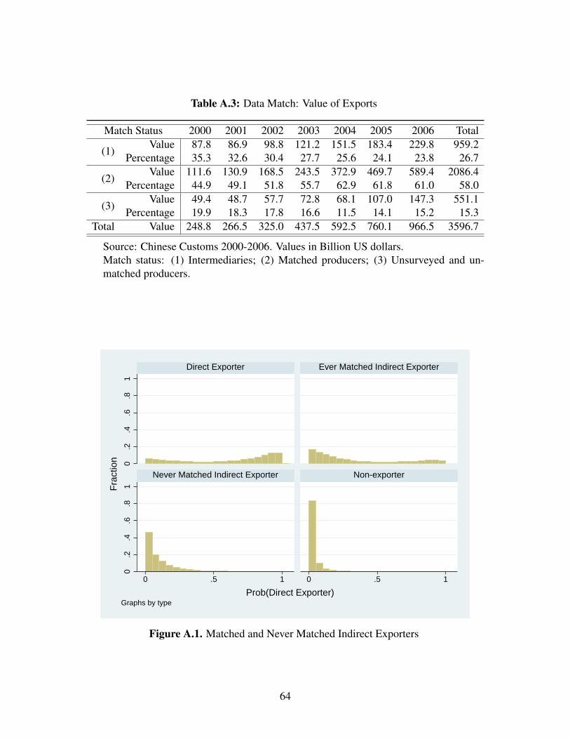
Table A.3: Data Match: Value of Exports

Match Status 2000 2001 2002 2003 2004 2005 2006 Total

(1)Value 87.8 86.9 98.8 121.2 151.5 183.4 229.8 959.2

Percentage 35.3 32.6 30.4 27.7 25.6 24.1 23.8 26.7

(2)Value 111.6 130.9 168.5 243.5 372.9 469.7 589.4 2086.4

Percentage 44.9 49.1 51.8 55.7 62.9 61.8 61.0 58.0

(3)Value 49.4 48.7 57.7 72.8 68.1 107.0 147.3 551.1

Percentage 19.9 18.3 17.8 16.6 11.5 14.1 15.2 15.3Total Value 248.8 266.5 325.0 437.5 592.5 760.1 966.5 3596.7

Source: Chinese Customs 2000-2006. Values in Billion US dollars.Match status: (1) Intermediaries; (2) Matched producers; (3) Unsurveyed and un-matched producers.

0.2

.4.6

.81

0.2

.4.6

.81

0 .5 1 0 .5 1

Direct Exporter Ever Matched Indirect Exporter

Never Matched Indirect Exporter Non-exporter

Fra

ctio

n

Prob(Direct Exporter)Graphs by type

Figure A.1. Matched and Never Matched Indirect Exporters

64

Tabl

eA

.4:P

rodu

ctiv

ityE

volu

tion:

Alte

rnat

ive

Prod

uctiv

ityM

easu

res

(1)

(2)

(3)

(4)

(5)

Ben

chm

ark

Torn

qvis

tT

FPR

TFP

VA

TFP

w/

TFP

Inde

xE

xtra

Con

trol

sC

onst

ant

α0

0.54

2***

0.38

2***

-1.9

85**

*0.

223*

**0.

620*

**(0

.032

)(0

.008

)(0

.028

)(0

.008

)(0

.035

)ωω ω

t−1

α1

0.30

3***

0.78

7***

-0.3

84**

*0.

781*

**0.

291*

**(0

.068

)(0

.009

)(0

.014

)(0

.008

)(0

.067

)ωω ω

2 t−1

α2

0.26

4***

0.03

9***

0.01

30.

054*

**0.

243*

**(0

.050

)(0

.004

)(0

.008

)(0

.006

)(0

.043

)ωω ω

3 t−1

α3

-0.0

28**

-0.0

09**

*0.

097*

**-0

.004

***

-0.0

25**

*(0

.012

)(0

.001

)(0

.003

)(0

.001

)(0

.008

)In

dire

ctE

xpor

t t−1

α4

0.00

7***

0.02

8***

-0.0

010.

017*

*0.

008*

**(0

.002

)(0

.010

)(0

.001

)(0

.007

)(0

.003

)D

irec

tExp

ort t−

1α

50.

025*

**0.

093*

**0.

004*

**0.

076*

**0.

028*

**(0

.002

)(0

.009

)(0

.001

)(0

.007

)(0

.003

)∗∗∗ ,∗∗

and∗

indi

cate

sign

ifica

nce

atth

e1%

,5%

and

10%

leve

l,re

spec

tivel

y.

65

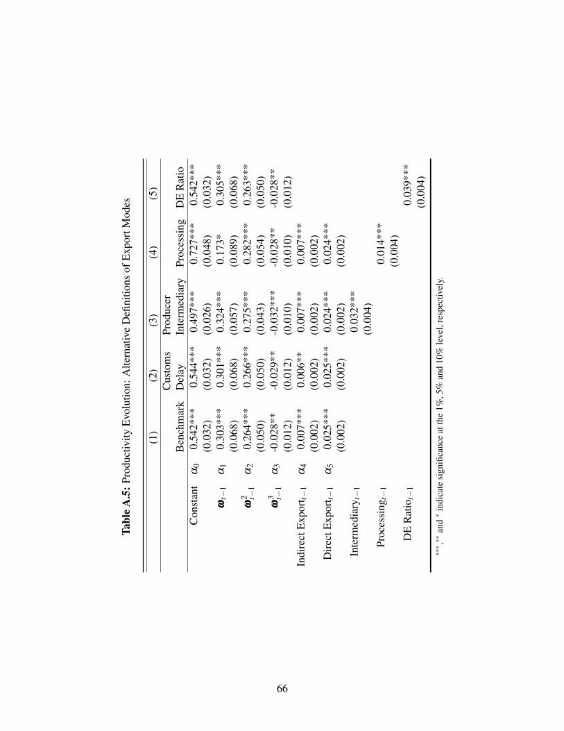
Tabl

eA

.5:P

rodu

ctiv

ityE

volu

tion:

Alte

rnat

ive

Defi

nitio

nsof

Exp

ortM

odes

(1)

(2)

(3)

(4)

(5)

Cus

tom

sPr

oduc

erB

ench

mar

kD

elay

Inte

rmed

iary

Proc

essi

ngD

ER

atio

Con

stan

tα

00.

542*

**0.

544*

**0.

497*

**0.

727*

**0.

542*

**(0

.032

)(0

.032

)(0

.026

)(0

.048

)(0

.032

)ωω ω

t−1

α1

0.30

3***

0.30

1***

0.32

4***

0.17

3*0.

305*

**(0

.068

)(0

.068

)(0

.057

)(0

.089

)(0

.068

)ωω ω

2 t−1

α2

0.26

4***

0.26

6***

0.27

5***

0.28

2***

0.26

3***

(0.0

50)

(0.0

50)

(0.0

43)

(0.0

54)

(0.0

50)

ωω ω3 t−

1α

3-0

.028

**-0

.029

**-0

.032

***

-0.0

28**

-0.0

28**

(0.0

12)

(0.0

12)

(0.0

10)

(0.0

10)

(0.0

12)

Indi

rect

Exp

ort t−

1α

40.

007*

**0.

006*

*0.

007*

**0.

007*

**(0

.002

)(0

.002

)(0

.002

)(0

.002

)D

irec

tExp

ort t−

1α

50.

025*

**0.

025*

**0.

024*

**0.

024*

**(0

.002

)(0

.002

)(0

.002

)(0

.002

)In

term

edia

ryt−

10.

032*

**(0

.004

)Pr

oces

sing

t−1

0.01

4***

(0.0

04)

DE

Rat

iot−

10.

039*

**(0

.004

)∗∗∗ ,∗∗

and∗

indi

cate

sign

ifica

nce

atth

e1%

,5%

and

10%

leve

l,re

spec

tivel

y.

66

Tabl

eA

.6:P

rodu

ctiv

ityE

volu

tion:

Prod

ucts

and

Des

tinat

ions

ofD

irec

tExp

ortin

g

(1)

(2)

(3)

(4)

(5)

Ben

chm

ark

GD

Pp/

cH

ong

Kon

gR

auch

Prob

(IE t−

1)C

onst

ant

α0

0.54

2***

0.57

7***

0.57

8***

0.57

7***

0.57

7***

(0.0

32)

(0.0

45)

(0.0

45)

(0.0

45)

(0.0

45)

ωω ωt−

1α

10.

303*

**0.

163*

0.16

3*0.

164*

0.16

4*(0

.068

)(0

.086

)(0

.086

)(0

.086

)(0

.086

)ωω ω

2 t−1

α2

0.26

4***

0.39

5***

0.39

5***

0.39

5***

0.39

5***

(0.0

50)

(0.0

57)

(0.0

57)

(0.0

57)

(0.0

57)

ωω ω3 t−

1α

3-0

.028

**-0

.061

***

-0.0

61**

*-0

.061

***

-0.0

61**

*(0

.012

)(0

.013

)(0

.013

)(0

.013

)(0

.013

)In

dire

ctE

xpor

t t−1

α4

0.00

7***

0.00

8***

0.00

8***

0.00

8***

0.00

8***

(0.0

02)

(0.0

03)

(0.0

03)

(0.0

03)

(0.0

03)

Dir

ectE

xpor

t t−1

α5

0.02

5***

0.02

1***

0.02

1***

0.01

4*0.

018*

**(0

.002

)(0

.004

)(0

.003

)(0

.008

)(0

.003

)R

ich

Des

tinat

ion*

DE t−

1-0

.002

(0.0

04)

Hon

gK

ong*

DE t−

1-0

.010

(0.0

10)

Diff

eren

tiate

dG

oods

*DE t−

10.

006

(0.0

08)

Prob

(IE t−

1)*D

E t−

10.

008

(0.0

08)

∗∗∗ ,∗∗

and∗

indi

cate

sign

ifica

nce

atth

e1%

,5%

and

10%

leve

l,re

spec

tivel

y.

67

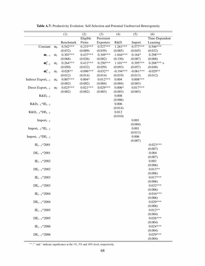
Table A.7: Productivity Evolution: Self-Selection and Potential Unobserved Heterogeneity

(1) (2) (3) (4) (5) (6)Eligible Persistent Time-Dependent

Benchmark Firms Exporters R&D Import LearningConstant α0 0.542*** 0.233*** 0.527*** 1.261*** 0.577*** 0.546***

(0.032) (0.009) (0.039) (0.085) (0.045) (0.032)ωωω t−1 α1 0.303*** 0.437*** 0.349*** -1.044*** 0.164* 0.298***

(0.068) (0.026) (0.082) (0.150) (0.087) (0.068)ωωω2

t−1 α2 0.264*** 0.412*** 0.250*** 1.101*** 0.395*** 0.268*** >(0.050) (0.032) (0.059) (0.093) (0.057) (0.048)

ωωω3t−1 α3 -0.028** -0.096*** -0.032** -0.194*** -0.061*** -0.029**

(0.012) (0.014) (0.014) (0.019) (0.013) (0.012)Indirect Exportt−1 α4 0.007*** 0.004* 0.012*** 0.004 0.008***

(0.002) (0.002) (0.004) (0.004) (0.003)Direct Exportt−1 α5 0.025*** 0.021*** 0.029*** 0.006* 0.017***

(0.002) (0.002) (0.003) (0.003) (0.003)R&Dt−1 0.008

(0.006)R&Dt−1*IEt−1 0.006

(0.014)R&Dt−1*DEt−1 0.012

(0.010)Importt−1 0.001

(0.004)Importt−1*IEt−1 0.001

(0.013)Importt−1*DEt−1 0.006

(0.007)IEt−1*2001 -0.023***

(0.007)DEt−1*2001 -0.004

(0.007)IEt−1*2002 0.003

(0.006)DEt−1*2002 0.013**

(0.006)IEt−1*2003 0.017***

(0.006)DEt−1*2003 0.032***

(0.006)IEt−1*2004 -0.016***

(0.006)DEt−1*2004 0.029***

(0.006)IEt−1*2005 0.012**

(0.004)DEt−1*2005 0.026***

(0.004)IEt−1*2006 0.024***

(0.004)DEt−1*2006 0.029***

(0.004)∗∗∗,∗∗ and ∗ indicate significance at the 1%, 5% and 10% level, respectively.

68