hp 9g graphing calculator contents
TRANSCRIPT
E-1
hp 9g Graphing Calculator Contents Chapter 1 : General Operations ................................... 4
Power Supply .................................................................... 4 Turning on or off ........................................................................... 4 Battery replacement ...................................................................... 4 Auto power-off function ................................................................ 4 Reset operation ............................................................................. 4
Contrast Adjustment .......................................................... 4 Display Features ................................................................ 5
Graph display............................................................................... 5 Calculation display........................................................................ 5
Chapter 2 : Before Starting a Calculation ...................... 6 Changing Modes ............................................................... 6 Selecting an Item from a Menu........................................... 6 Key Labels......................................................................... 6 Using the 2nd and ALPHA keys .......................................... 7 Cursor .............................................................................. 7 Inserting and Deleting Characters....................................... 7 Recalling Previous Inputs and Results .................................. 8 Memory............................................................................ 8
Running memory........................................................................... 8 Standard memory variables .......................................................... 8 Storing an equation ...................................................................... 8 Array Variables............................................................................. 8
Order of Operations .......................................................... 9 Accuracy and Capacity .................................................... 10 Error Conditions .............................................................. 12
Chapter 3 : Basic Calculations .................................... 13 Arithmetic Calculation...................................................... 13
E-2
Display Format ................................................................ 13 Parentheses Calculations .................................................. 14 Percentage Calculations ................................................... 14 Repeat Calculations ......................................................... 14 Answer Function.............................................................. 14
Chapter 4 : Common Math Calculations...................... 15 Logarithm and Antilogarithm ........................................... 15 Fraction Calculation ......................................................... 15 Converting Angular Units ................................................. 15 Trigonometric and Inverse Trigonometric functions............. 16 Hyperbolic and Inverse Hyperbolic functions ..................... 16 Coordinate Transformations ............................................. 16 Mathematical Functions ................................................... 16 Other Functions ( x-1, , , ,x 2, x 3, ^ ).................... 17 Unit Conversion............................................................... 17 Physics Constants ............................................................ 18 Multi-statement functions ................................................. 19
Chapter 5 : Graphs .................................................... 19 Built-in Function Graphs................................................... 19 User-generated Graphs .................................................... 19 Graph ↔ Text Display and Clearing a Graph.................... 20 Zoom Function ................................................................ 20 Superimposing Graphs .................................................... 20 Trace Function ................................................................. 20 Scrolling Graphs.............................................................. 21 Plot and Line Function ...................................................... 21
Chapter 6 : Statistical Calculations.............................. 21 Single-Variable and Two-Variable Statistics....................... 21 Process Capability ........................................................... 22 Correcting Statistical Data ................................................ 23
E-3
Probability Distribution (1-Var Data) ................................. 23 Regression Calculation..................................................... 24
Chapter 7 : BaseN Calculations .................................. 24 Negative Expressions....................................................... 25 Basic Arithmetic Operations for Bases............................... 25 Logical Operation............................................................ 25
Chapter 8 : Programming........................................... 25 Before Using the Program Area ........................................ 26 Program Control Instructions ............................................ 26
Clear screen command.................................................................26 Input and output commands.........................................................26 Conditional branching..................................................................27 Jump commands ..........................................................................27 Mainroutine and Subroutine.........................................................27 Increment and decrement............................................................ 28 For loop ...................................................................................... 28 Sleep command .......................................................................... 28 Swap command .......................................................................... 28
Relational Operators........................................................ 29 Creating a New Program ................................................. 29 Executing a Program ....................................................... 29 Debugging a Program ..................................................... 30 Using the Graph Function in Programs.............................. 30 Display Result Command.................................................. 30 Deleting a Program ......................................................... 30 Program Examples .......................................................... 31
E-4
Chapter 1 : General Operations
Power Supply
Turning on or off To turn the calculator on, press [ ON ].
To turn the calculator off, press [ 2nd ] [ OFF ].
Battery replacement The calculator is powered by two alkaline button batteries (GP76A or LR44). When battery power becomes low, LOW BATTERY appears on the display. Replace the batteries as soon as possible.
To replace the batteries:
1. Remove the battery compartment cover by sliding it in the direction of the arrow.
2. Remove the old batteries. 3. Install new batteries, each with positive polarity facing outward. 4. Replace the battery compartment cover. 5. Press [ ON ] to turn the power on. Auto power-off function The calculator automatically turns off if it has not been used for 9–15 minutes. It can be reactivated by pressing [ ON ]. The display, memory, and settings are retained while the calculator is off.
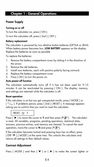
Reset operation If the calculator is on but you get unexpected results, press [ MODE ] or [ CL/ESC ]. If problems persist, press [ 2nd ] [ RESET ]. A message appears asking you to confirm that you want to reset the calculator.
RESET : N Y
Press [ ] to move the cursor to Y and then press [ ]. The calculator is reset. All variables, programs, pending operations, statistical data, answers, previous entries, and memory are cleared. To cancel the reset operation, move the cursor to N and press [ ].
If the calculator becomes locked and pressing keys has no effect, press [ EXP ] [ MODE ] at the same time. This unlocks the calculator and returns all settings to their default values.
Contrast Adjustment
Press [ MODE ] and then [ ] or [ ] to make the screen lighter or
E-5
darker.
Display Features
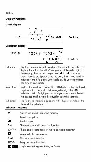
Graph display
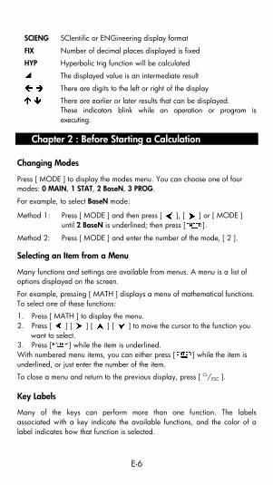
Calculation display
Entry line Displays an entry of up to 76 digits. Entries with more than 11 digits will scroll to the left. When you input the 69th digit of a single entry, the cursor changes from to to let you know that you are approaching the entry limit. If you need to input more than 76 digits, you should divide your calculation into two or more parts.
Result line Displays the result of a calculation. 10 digits can be displayed, together with a decimal point, a negative sign, the x10 indicator, and a 2-digit positive or negative exponent. Results that exceed this limit are displayed in scientific notation.
Indicators The following indicators appear on the display to indicate the status of the calculator.
Indicator Meaning
M Values are stored in running memory
– Result is negative
Invalid action
2nd The next action will be a 2nd function
X = Y = The x- and y-coordinates of the trace function pointer
Alphabetic keys are active
STAT Statistics mode is active
PROG Program mode is active
Angle mode: Degrees, Rads, or Grads
E-6
SCIENG SCIentific or ENGineering display format
FIX Number of decimal places displayed is fixed
HYP Hyperbolic trig function will be calculated
The displayed value is an intermediate result
There are digits to the left or right of the display
There are earlier or later results that can be displayed. These indicators blink while an operation or program is executing.
Chapter 2 : Before Starting a Calculation
Changing Modes
Press [ MODE ] to display the modes menu. You can choose one of four modes: 0 MAIN, 1 STAT, 2 BaseN, 3 PROG.
For example, to select BaseN mode:
Method 1: Press [ MODE ] and then press [ ], [ ] or [ MODE ] until 2 BaseN is underlined; then press [ ].
Method 2: Press [ MODE ] and enter the number of the mode, [ 2 ].
Selecting an Item from a Menu
Many functions and settings are available from menus. A menu is a list of options displayed on the screen.
For example, pressing [ MATH ] displays a menu of mathematical functions. To select one of these functions:
1. Press [ MATH ] to display the menu. 2. Press [ ] [ ] [ ] [ ] to move the cursor to the function you
want to select. 3. Press [ ] while the item is underlined. With numbered menu items, you can either press [ ] while the item is underlined, or just enter the number of the item.
To close a menu and return to the previous display, press [ CL/ESC ].
Key Labels
Many of the keys can perform more than one function. The labels associated with a key indicate the available functions, and the color of a label indicates how that function is selected.
E-7
Label color Meaning
White Just press the key
Yellow Press [ 2nd ] and then the key
Green In Base-N mode, just press the key
Blue Press [ ALPHA ] and then the key
Using the 2nd and ALPHA keys
To execute a function with a yellow label, press [ 2nd ] and then the corresponding key. When you press [ 2nd ], the 2nd indicator appears to indicate that you will be selecting the second function of the next key you press. If you press [ 2nd ] by mistake, press [ 2nd ] again to remove the 2nd indicator
Pressing [ ALPHA ] [ 2nd ] locks the calculator in 2nd function mode. This allows consecutive input of 2nd function keys. To cancel this, press [ 2nd ] again.
To execute a function with a blue label, press [ ALPHA ] and then the corresponding key. When you press [ ALPHA ], the indicator appears to indicate that you will be selecting the alphabetic function of the next key you press. If you press [ ALPHA ] by mistake, press [ ALPHA ] again to remove the indicator.
Pressing [ 2nd ] [ ALPHA ] locks the calculator in alphabetic mode. This allows consecutive input of alphabetic function keys. To cancel this, press [ ALPHA ] again.
Cursor
Press [ ] or [ ] to move the cursor to the left or the right. Hold down a cursor key to move the cursor quickly.
If there are entries or results not visible on the display, press [ ] or [ ] to scroll the display up or down. You can reuse or edit a previous entry when it is on the entry line.
Press [ ALPHA ] [ ] or [ ALPHA ] [ ] to move the cursor to the beginning or the end of the entry line. Press [ ALPHA ] [ ] or [ ALPHA ] [ ] to move the cursor to the top or bottom of all entries.
The blinking cursor indicates that the calculator is in insert mode.
Inserting and Deleting Characters
To insert a character, move the cursor to the appropriate position and enter the character. The character is inserted to the immediate left of the cursor.
E-8
To delete a character, press [ ] or [ ] to move the cursor to that character and then press [ DEL ]. (When the cursor is on a character, the character is underlined.) To undo the deletion, immediately press [ 2nd ] [ ].
To clear all characters, press [ CL/ESC ]. See Example 1.
Recalling Previous Inputs and Results
Press [ ] or [ ] to display up to 252 characters of previous input, values and commands, which can be modified and re-executed. See Example 2.
Note: Previous input is not cleared when you press [ CL/ESC ] or the power is turned off` but it is cleared when you change modes.
Memory
Running memory Press [ M+ ] to add a result to running memory. Press [ 2nd ] [ M– ] to subtract the value from running memory. To recall the value in running memory, press [ MRC ]. To clear running memory, press [ MRC ] twice. See Example 4.
Standard memory variables The calculator has 26 standard memory variables—A, B, C, D, …, Z—which you can use to assign a value to. See Example 5. Operations with variables include:
• [ SAVE ] + Variable assigns the current answer to the specified variable (A, B, C, … or Z).
• [ 2nd ] [ RCL ] displays a menu of variables; select a variable to recall its value.
• [ ALPHA ] + Variable recalls the value assigned to the specified variable.
• [ 2nd ] [ CL-VAR ] clears all variables.
Note: You can assign the same value to more than one variable in one step. For example, to assign 98 to variables A, B, C and D, press 98 [ SAVE ] [ A ] [ ALPHA ] [ ~ ] [ ALPHA ] [ D ].
Storing an equation Press [ SAVE ] [ PROG ] to store the current equation in memory.
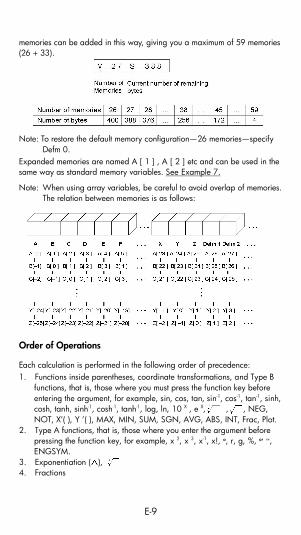
Press [ PROG ] to recall the equation. See Example 6. Array Variables In addition to the 26 standard memory variables (see above), you can increase memory storage by converting program steps to memory variables. You can convert 12 program steps to one memory. A maximum of 33
E-9
memories can be added in this way, giving you a maximum of 59 memories (26 + 33). Note: To restore the default memory configuration—26 memories—specify
Defm 0. Expanded memories are named A [ 1 ] , A [ 2 ] etc and can be used in the same way as standard memory variables. See Example 7.
Note: When using array variables, be careful to avoid overlap of memories. The relation between memories is as follows:
Order of Operations
Each calculation is performed in the following order of precedence: 1. Functions inside parentheses, coordinate transformations, and Type B
functions, that is, those where you must press the function key before entering the argument, for example, sin, cos, tan, sin-1, cos-1, tan-1, sinh, cosh, tanh, sinh-1, cosh-1, tanh-1, log, ln, 10 X , e X, , , NEG, NOT, X’( ), Y ’( ), MAX, MIN, SUM, SGN, AVG, ABS, INT, Frac, Plot.
2. Type A functions, that is, those where you enter the argument before pressing the function key, for example, x 2, x 3, x-1, x!, º, r, g, %, º΄ ΄΄, ENGSYM.
3. Exponentiation ( ), 4. Fractions
E-10
5. Abbreviated multiplication format involving variables, π, RAND, RANDI.
6. ( – ) 7. Abbreviated multiplication format in front of Type B functions, ,
Alog2, etc. 8. nPr, nCr 9. × , 10. +, – 11. Relational operators: = =, < , >, ≠, ≤ , ≥ 12. AND, NAND (BaseN calculations only) 13. OR, XOR, XNOR (BaseN calculations only) 14. Conversion (A b/c d/e, F D, DMS) When functions with the same priority are used in series, execution is performed from right to left. For example:
e X ln120 → e X { ln (120 ) }
Otherwise, execution is from left to right.
Compound functions are executed from right to left.
Accuracy and Capacity
Output digits: Up to 10 digits
Calculating digits: Up to 24 digits Where possible, every calculation is displayed in up to 10 digits, or as a 10-digit mantissa together with a 2-digit exponent up to 10 ±99.
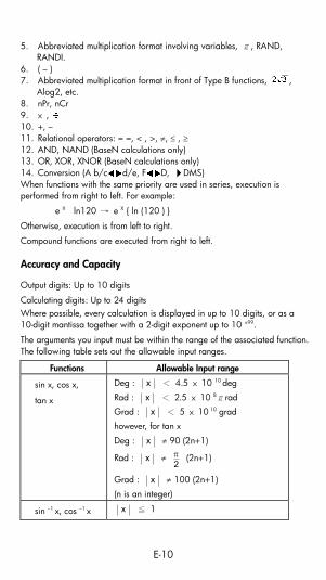
The arguments you input must be within the range of the associated function. The following table sets out the allowable input ranges.
Functions Allowable Input range
sin x, cos x,
tan x
Deg : x < 4.5 × 10 10 deg
Rad : x < 2.5 × 10 8πrad
Grad : x < 5 × 10 10 grad
however, for tan x
Deg : x ≠ 90 (2n+1)
Rad : x ≠ 2π (2n+1)
Grad : x ≠ 100 (2n+1)
(n is an integer)
sin –1 x, cos –1 x x ≦ 1
E-11
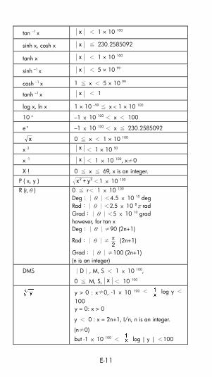
tan –1 x x < 1 × 10 100
sinh x, cosh x x ≦ 230.2585092
tanh x x < 1 × 10 100
sinh –1 x x < 5 × 10 99
cosh –1 x 1 ≦ x < 5 × 10 99
tanh –1 x x < 1
log x, ln x 1 × 10 –99 ≦ x < 1 × 10 100
10 x –1 × 10 100 < x < 100
e x –1 × 10 100 < x ≦ 230.2585092
x 0 ≦ x < 1 × 10 100
x 2 x < 1 × 10 50
x -1 x < 1 × 10 100, x≠0
X ! 0 ≦ x ≦ 69, x is an integer.
P ( x, y ) 22 y+x <1 × 10 100 R (r,θ) 0 ≦ r< 1 × 10 100
Deg:│θ│<4.5 × 10 10 deg Rad:│θ│<2.5 × 10 8πrad Grad:│θ│<5 × 10 10 grad however, for tan x Deg:│θ│≠90 (2n+1)
Rad:│θ│≠2π (2n+1)
Grad:│θ│≠100 (2n+1) (n is an integer)
DMS │D│, M, S < 1 × 10 100,
0 ≦ M, S, x < 10 100
y > 0 : x≠0, -1 × 10 100 < log y <
100 y = 0: x > 0
y < 0 : x = 2n+1, I/n, n is an integer.
(n≠0)
but -1 × 10 100 < log | y | <100
E-12
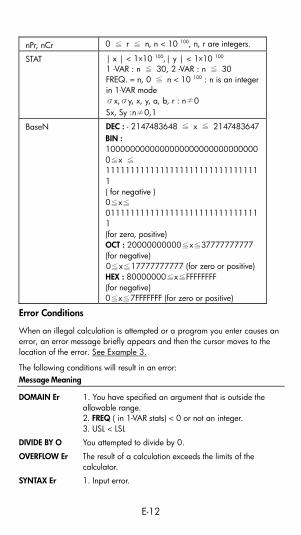
nPr, nCr 0 ≦ r ≦ n, n < 10 100, n, r are integers.
STAT | x | < 1×10 100,| y | < 1×10 100 1 -VAR : n ≦ 30, 2 -VAR : n ≦ 30 FREQ. = n, 0 ≦ n < 10 100 : n is an integer in 1-VAR mode σx,σy, x, y, a, b, r : n≠0 Sx, Sy :n≠0,1
BaseN DEC : - 2147483648 ≦ x ≦ 2147483647BIN : 10000000000000000000000000000000≦x ≦11111111111111111111111111111111 ( for negative ) 0≦x≦01111111111111111111111111111111 (for zero, positive) OCT : 20000000000≦x≦37777777777 (for negative) 0≦x≦17777777777 (for zero or positive) HEX : 80000000≦x≦FFFFFFFF (for negative) 0≦x≦7FFFFFFF (for zero or positive)
Error Conditions
When an illegal calculation is attempted or a program you enter causes an error, an error message briefly appears and then the cursor moves to the location of the error. See Example 3.
The following conditions will result in an error: Message Meaning
DOMAIN Er 1. You have specified an argument that is outside the allowable range. 2. FREQ ( in 1-VAR stats) < 0 or not an integer. 3. USL < LSL
DIVIDE BY O You attempted to divide by 0.
OVERFLOW Er The result of a calculation exceeds the limits of the calculator.
SYNTAX Er 1. Input error.
E-13
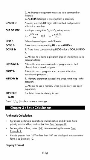
2. An improper argument was used in a command or function. 3. An END statement is missing from a program.
LENGTH Er An entry exceeds 84 digits after implied multiplication with auto-correction.
OUT OF SPEC You input a negative CPU or CPL value, where
σ3
x–USL=CPU and σ3LSL–x=C
PL
NEST Er Subroutine nesting exceeds 3 levels.
GOTO Er There is no corresponding Lbl n for a GOTO n.
GOSUB Er 1. There is no corresponding PROG n for a GOSUB PROG n.
2. Attempt to jump to a program area in which there is no program stored.
EQN SAVE Er Attempt to save an equation to a program area that already has a stored program.
EMPTY Er Attempt to run a program from an area without an equation or program.
MEMORY Er 1. Memory expansion exceeds the steps remaining in the program.
2. Attempt to use a memory when no memory has been expanded.
DUPLICATE The label name is already in use.
LABEL
Press [ CL/ESC ] to clear an error message.
Chapter 3 : Basic Calculations
Arithmetic Calculation
• For mixed arithmetic operations, multiplication and division have priority over addition and subtraction. See Example 8.
• For negative values, press [ (–) ] before entering the value. See Example 9.
• Results greater than 1010 or less than 10-9 are displayed in exponential form. See Example 10.
Display Format
E-14
• A decimal format is selected by pressing [ 2nd ] [ FIX ] and selecting a value from the menu (F0123456789). To set the displayed decimal places to n, enter a value for n directly, or press the cursor keys until the value is underlined and then press [ ]. (The default setting is floating point notation (F) and its n value is •). See Example 11.
• Number display formats are selected by pressing [ 2nd ] [ SCI/ENG ] and choosing a format from the menu. The items on the menu are FLO (for floating point), SCI (for scientific), and ENG (for engineering). Press [ ] or [ ] until the desired format is underlined, and then press [ ]. See Example 12.
• You can enter a number in mantissa and exponent format using the [ EXP ] key. See Example 13.
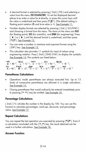
• This calculator also provides 11 symbols for input of values using engineering notation. Press [ 2nd ] [ ENG SYM ] to display the symbols. See Example 14. The symbols are listed below:
Parentheses Calculations
• Operations inside parentheses are always executed first. Up to 13 levels of consecutive parentheses are allowed in a single calculation. See Example 15.
• Closing parentheses that would ordinarily be entered immediately prior to pressing [ ] may be omitted. See Example 16.
Percentage Calculations
[ 2nd ] [ % ] divides the number in the display by 100. You can use this function to calculate percentages, mark-ups, discounts, and percentage ratios. See Example 17.
Repeat Calculations
You can repeat the last operation you executed by pressing [ ]. Even if a calculation concluded with the [ ] key, the result obtained can be used in a further calculation. See Example 18.
Answer Function
E-15
When you enter a numeric value or numeric expression and press [ ], the result is stored in the Answer function, which you can then quickly recall. See Example 19.
Note: The result is retained even if the power is turned off. It is also retained if a subsequent calculation results in an error.
Chapter 4 : Common Math Calculations
Logarithm and Antilogarithm
You can calculate common and natural logarithms and antilogarithms using [ log ], [ ln ], [ 2nd ] [ 10 x ], and [ 2nd ] [ e x ]. See Example 20.
Fraction Calculation
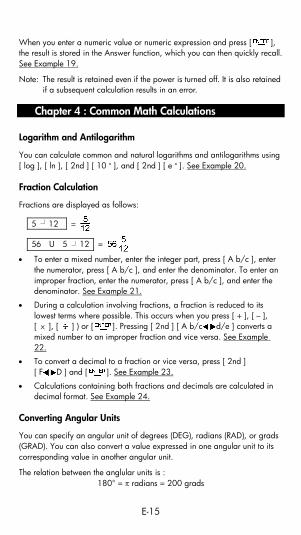
Fractions are displayed as follows:
5 ┘12 =
56 U 5 ┘12 =
• To enter a mixed number, enter the integer part, press [ A b/c ], enter the numerator, press [ A b/c ], and enter the denominator. To enter an improper fraction, enter the numerator, press [ A b/c ], and enter the denominator. See Example 21.
• During a calculation involving fractions, a fraction is reduced to its lowest terms where possible. This occurs when you press [ + ], [ – ], [ × ], [ ] ) or [ ]. Pressing [ 2nd ] [ A b/c d/e ] converts a mixed number to an improper fraction and vice versa. See Example 22.
• To convert a decimal to a fraction or vice versa, press [ 2nd ] [ F D ] and [ ]. See Example 23.
• Calculations containing both fractions and decimals are calculated in decimal format. See Example 24.
Converting Angular Units
You can specify an angular unit of degrees (DEG), radians (RAD), or grads (GRAD). You can also convert a value expressed in one angular unit to its corresponding value in another angular unit.
The relation between the anglular units is : 180° = π radians = 200 grads
E-16
To change the angular unit setting to another setting, press [ DRG ] repeatedly until the angular unit you want is indicated on the display.
The conversion procedure follows (also see Example 25): 1. Change the angle units to the units you want to convert to. 2. Enter the value of the unit to convert. 3. Press [ 2nd ] [ DMS ] to display the menu. The units you can select are
°(degrees), ’ (minutes), ” (seconds), r (radians), g (gradians) or DMS (Degrees-Minutes-Seconds).
4. Select the units you are converting from. 5. Press [ ] twice. To convert an angle to DMS notation, select DMS. An example of DMS notation is 1° 30’ 0” (= 1 degrees, 30 minutes, 0 seconds). See Example 26.
To convert from DMS notation to decimal notation, select °(degrees), ’(minutes), ”(seconds). See Example 27.
Trigonometric and Inverse Trigonometric functions
The calculator provides standard trigonometric functions and inverse trigonometric functions: sin, cos, tan, sin-1, cos-1 and tan-1. See Example 28.
Note: Before undertaking a trigonometric or inverse trigonometric calculation, make sure that the appropriate angular unit is set.
Hyperbolic and Inverse Hyperbolic functions
The [ 2nd ] [ HYP ] keys are used to initiate hyperbolic and inverse hyperbolic calculations using sinh, cosh, tanh, sinh-1, cosh-1 and tanh-1. See Example 29.
Note: Before undertaking a hyperbolic or inverse hyperbolic calculation, make sure that the appropriate angular unit is set.
Coordinate Transformations
Press [ 2nd ] [ R P ] to display a menu to convert rectangular coordinates to polar coordinates or vice versa. See Example 30.
Note: Before undertaking a coordinate transformation, make sure that the appropriate angular unit is set.
Mathematical Functions
E-17
Press [ MATH ] repeatedly to is display a list of mathematical functions and their associated arguments. See Example 31. The functions available are:
! Calculate the factorial of a specified positive integer n , where n≦69.
RAND Generate a random number between 0 and 1.
RANDI Generate a random integer between two specified integers, A and B, where A ≦ random value≦ B.
RND Round off the result.
MAX Determine the maximum of given numbers. (Up to 10 numbers can be specified.)
MIN Determine the minimum of given numbers. (Up to 10 numbers can be specified.)
SUM Determine the sum of given numbers. (Up to 10 numbers can be specified.)
AVG Determine the average of given numbers. (Up to 10 numbers can be specified.)
Frac Determine the fractional part of a given number.
INT Determine the integer part of a given number.
SGN Indicate the sign of a given number: if the number is negative, –1 is displayed; if zero, 0 is displayed; if positive, 1 is displayed.
ABS Display the absolute value of a given number.
nPr Calculate the number of possible permutations of n items taken r at a time.
nCr Calculate the number of possible combinations of n items taken r at a time.
Defm Memory expansion.
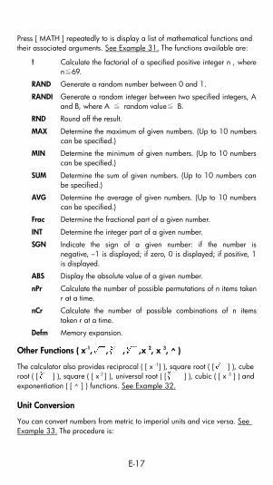
Other Functions ( x-1, , , ,x 2, x 3, ^ )
The calculator also provides reciprocal ( [ x -1] ), square root ( [ ] ), cube root ( [ ] ), square ( [ x 2 ] ), universal root ( [ ] ), cubic ( [ x 3 ] ) and exponentiation ( [ ^ ] ) functions. See Example 32.
Unit Conversion
You can convert numbers from metric to imperial units and vice versa. See Example 33. The procedure is:
E-18
1. Enter the number you want to convert. 2. Press [ 2nd ] [ CONV ] to display the units menu. There are 7 menus,
covering distance, area, temperature, capacity, weight, energy, and pressure.
3. Press [ ] or [ ] to scroll through the list of units until the appropriate units menu is shown, then press [ ] .
4. Press [ ] or [ ] to convert the number to the highlighted unit.
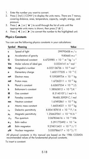
Physics Constants
You can use the following physics constants in your calculations:
Symbol Meaning Value
c Speed of light 299792458 m / s
g Acceleration of gravity 9.80665 m.s -2
G Gravitational constant 6.6725985 × 10 -11 m 3 kg -1 s -2
Vm Molar volume of ideal gas 0.0224141 m 3 mol -1
NA Avogadro’s number 6.022136736 × 10 23 mol -1
e Elementary charge 1.602177335 × 10 -19 C
me Electron mass 9.109389754 × 10 -31 kg
mp Proton mass 1.67262311 × 10 -27 kg
h Planck’s constant 6.62607554 × 10 -34 J.S
k Boltzmann’s constant 1.38065812 × 10 -23J.K -1
IR Gas constant 8.3145107 J / mol • k
IF Faraday constant 96485.30929 C / mol
mn Neutron constant 1.67492861 × 10 -27 kg
µ Atomic mass constant 1.66054021 × 10 -27 kg
ε0 Dielectric permittivity 8.854187818 × 10 -12 F / m
µ0 Magnetic permittivity 1.256637061 × 10 -6 N A -2 φ0 Flux quantum 2.067834616 × 10 -15 Wb
a 0 Bohr radius 5.291772492 × 10 -11m
µB Bohr magneton 9.274015431 × 10 -24 J / T
µN Nuclear magneton 5.050786617 × 10 -27J / T
All physical constants in this manual are based on the 1986 CODATA recommended values of the fundamental physical constants.
To insert a constant:
E-19
1. Position your cursor where you want the constant inserted. 2. Press [ 2nd ] [ CONST ] to display the physics constants menu. 3. Scroll through the menu until the constant you want is underlined. 4. Press [ ]. (See Example 34.)
Multi-statement functions
Multi-statement functions are formed by connecting a number of individual statements for sequential execution. You can use multi-statements in manual calculations and in the program calculations.
When execution reaches the end of a statement that is followed by the display result command symbol ( ), execution stops and the result up to that point appears on the display. You can resume execution by pressing [ ]. See Example 35.
Chapter 5 : Graphs
Built-in Function Graphs
You can produce graphs of the following functions: sin, cos, tan, sin -1, cos -1, tan -1, sinh, cosh, tanh, sinh -1, cosh -1, tanh -1, , , x 2 , x 3 , log, ln, 10
x, e x, x –1. When you generate a built-in graph, any previously generated graph is cleared. The display range is automatically set to the optimum. See Example 36.
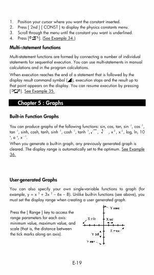
User-generated Graphs
You can also specify your own single-variable functions to graph (for example, y = x 3 + 3x 2 – 6x – 8). Unlike built-in functions (see above), you must set the display range when creating a user generated graph.
Press the [ Range ] key to access the range parameters for each axis: minimum value, maximum value, and scale (that is, the distance between the tick marks along an axis).
E-20
After setting the range, press [ Graph ] and enter the expression to be graphed. See Example 37.
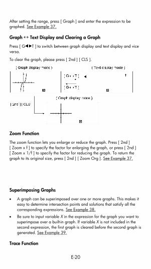
Graph ↔ Text Display and Clearing a Graph
Press [ G T ] to switch between graph display and text display and vice versa.
To clear the graph, please press [ 2nd ] [ CLS ].
Zoom Function
The zoom function lets you enlarge or reduce the graph. Press [ 2nd ] [ Zoom x f ] to specify the factor for enlarging the graph, or press [ 2nd ] [ Zoom x 1/f ] to specify the factor for reducing the graph. To return the graph to its original size, press [ 2nd ] [ Zoom Org ]. See Example 37.
Superimposing Graphs
• A graph can be superimposed over one or more graphs. This makes it easy to determine intersection points and solutions that satisfy all the corresponding expressions. See Example 38.
• Be sure to input variable X in the expression for the graph you want to superimpose over a built-in graph. If variable X is not included in the second expression, the first graph is cleared before the second graph is generated. See Example 39.
Trace Function

E-21
This function lets you move a pointer around a graph by pressing [ ] and [ ]. The x- and y-coordinates of the current pointer location are displayed on the screen. This function is useful for determining the intersection of superimposed graphs (by pressing [ 2nd ] [ X Y ]). See Example 40.
Note: Due to the limited resolution of the display, the position of the pointer may be an approximation.
Scrolling Graphs
After generating a graph, you can scroll it on the display. Press [ ] [ ] [ ] [ ] to scroll the graph left, right, up or down respectively. See Example 41.
Plot and Line Function
The plot function is used to mark a point on the screen of a graph display. The point can be moved left, right, up, or down using the cursor keys. The coordinates of the point are displayed.
When the pointer is at the desired location, press [ 2nd ] [ PLOT ] to plot a point. The point blinks at the plotted location.
Two points can be connected by a straight line by pressing [ 2nd ] [ LINE ]. See Example 42.
Chapter 6 : Statistical Calculations
The statistics menu has four options: 1-VAR (for analyzing data in a single dataset), 2-VAR (for analyzing paired data from two datasets), REG (for performing regression calculations), and D-CL (for clearing all datasets).
Single-Variable and Two-Variable Statistics
1. From the statistics menu, choose 1-VAR or 2-VAR and press [ ]. 2. Press [ DATA ], select DATA-INPUT from the menu and press [ ]. 3. Enter an x value and press [ ]. 4. Enter the frequency ( FREQ ) of the x value (in 1-VAR mode) or the
corresponding y value ( in 2-VAR mode ) and press [ ]. 5. To enter more data, repeat from step 3. 6. Press [ 2nd ] [ STATVAR ].
E-22
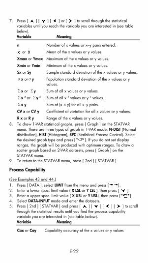
7. Press [ ] [ ] [ ] or [ ] to scroll through the statistical variables until you reach the variable you are interested in (see table below). Variable Meaning
n Number of x values or x–y pairs entered.
or Mean of the x values or y values.
Xmax or Ymax Maximum of the x values or y values.
Xmin or Ymin Minimum of the x values or y values.
Sx or Sy Sample standard deviation of the x values or y values.
σx orσy Population standard deviation of the x values or y values.
Σx or Σy Sum of all x values or y values.
Σx 2 or Σy 2 Sum of all x 2 values or y 2 values. Σx y Sum of (x × y) for all x–y pairs.
CV x or CV y Coefficient of variation for all x values or y values.
R x or R y Range of the x values or y values. 8. To draw 1-VAR statistical graphs, press [ Graph ] on the STATVAR
menu. There are three types of graph in 1-VAR mode: N-DIST (Normal distribution), HIST (Histogram), SPC (Statistical Process Control). Select the desired graph type and press [ ]. If you do not set display ranges, the graph will be produced with optimum ranges. To draw a scatter graph based on 2-VAR datasets, press [ Graph ] on the STATVAR menu.
9. To return to the STATVAR menu, press [ 2nd ] [ STATVAR ].
Process Capability
(See Examples 43 and 44.) 1. Press [ DATA ], select LIMIT from the menu and press [ ]. 2. Enter a lower spec. limit value ( X LSL or Y LSL ), then press [ ]. 3. Enter a upper spec. limit value ( X USL or Y USL), then press [ ] . 4. Select DATA-INPUT mode and enter the datasets. 5. Press [ 2nd ] [ STATVAR ] and press [ ] [ ] [ ] [ ] to scroll
through the statistical results until you find the process capability variable you are interested in (see table below). Variable Meaning
Cax or Cay Capability accuracy of the x values or y values
E-23
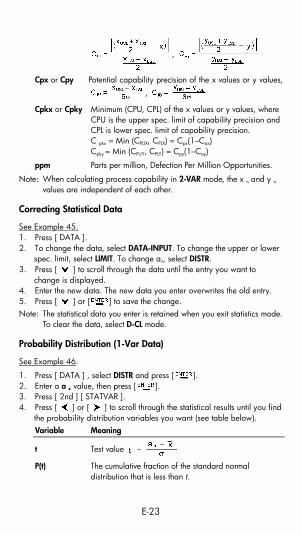
,
Cpx or Cpy Potential capability precision of the x values or y values, ,
Cpkx or Cpky Minimum (CPU, CPL) of the x values or y values, where CPU is the upper spec. limit of capability precision and CPL is lower spec. limit of capability precision. C pkx = Min (CPUX, CPLX) = Cpx(1–Cax) Cpky = Min (CPUY, CPLY) = Cpy(1–Cay)
ppm Parts per million, Defection Per Million Opportunities.
Note: When calculating process capability in 2-VAR mode, the x n and y n values are independent of each other.
Correcting Statistical Data
See Example 45. 1. Press [ DATA ]. 2. To change the data, select DATA-INPUT. To change the upper or lower
spec. limit, select LIMIT. To change ax, select DISTR. 3. Press [ ] to scroll through the data until the entry you want to
change is displayed. 4. Enter the new data. The new data you enter overwrites the old entry. 5. Press [ ] or [ ] to save the change. Note: The statistical data you enter is retained when you exit statistics mode.
To clear the data, select D-CL mode.
Probability Distribution (1-Var Data)
See Example 46.
1. Press [ DATA ] , select DISTR and press [ ]. 2. Enter a a x value, then press [ ]. 3. Press [ 2nd ] [ STATVAR ]. 4. Press [ ] or [ ] to scroll through the statistical results until you find
the probability distribution variables you want (see table below). Variable Meaning
t Test value
P(t) The cumulative fraction of the standard normal distribution that is less than t.
E-24
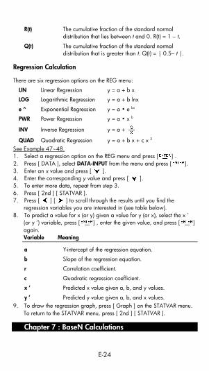
R(t) The cumulative fraction of the standard normal distribution that lies between t and 0. R(t) = 1 – t.
Q(t) The cumulative fraction of the standard normal distribution that is greater than t. Q(t) = | 0.5– t |.
Regression Calculation
There are six regression options on the REG menu:
LIN Linear Regression y = a + b x
LOG Logarithmic Regression y = a + b lnx
e ^ Exponential Regression y = a • e bx
PWR Power Regression y = a • x b
INV Inverse Regression y = a +
QUAD Quadratic Regression y = a + b x + c x 2 See Example 47~48. 1. Select a regression option on the REG menu and press [ ] . 2. Press [ DATA ], select DATA-INPUT from the menu and press [ ]. 3. Enter an x value and press [ ]. 4. Enter the corresponding y value and press [ ]. 5. To enter more data, repeat from step 3. 6. Press [ 2nd ] [ STATVAR ]. 7. Press [ ] [ ] to scroll through the results until you find the
regression variables you are interested in (see table below). 8. To predict a value for x (or y) given a value for y (or x), select the x ’
(or y ’) variable, press [ ] , enter the given value, and press [ ] again. Variable Meaning
a Y-intercept of the regression equation.
b Slope of the regression equation.
r Correlation coefficient.
c Quadratic regression coefficient.
x ’ Predicted x value given a, b, and y values.
y ’ Predicted y value given a, b, and x values. 9. To draw the regression graph, press [ Graph ] on the STATVAR menu.
To return to the STATVAR menu, press [ 2nd ] [ STATVAR ].
Chapter 7 : BaseN Calculations
E-25
You can enter numbers in base 2, base 8, base 10 or base 16. To set the number base, press [ 2nd ] [ dhbo ], select an option from the menu and press [ ]. An indicator shows the base you selected: d, h, b , or o. (The default setting is d: decimal base). See Example 49.
The allowable digits in each base are:
Binary base (b): 0, 1
Octal base (o): 0, 1, 2, 3, 4, 5, 6, 7
Decimal base (d): 0, 1, 2, 3, 4, 5, 6, 7, 8, 9
Hexadecimal base (h): 0, 1, 2, 3, 4, 5, 6, 7, 8, 9, IA, IB, IC, ID, IE, IF
Note: To enter a number in a base other than the set base, append the corresponding designator (d, h, b, o) to the number (as in h3).
Press [ ] to use the block function, which displays a result in octal or binary base if it exceeds 8 digits. Up to 4 blocks can be displayed. See Example 50.
Negative Expressions
In binary, octal, and hexadecimal bases, negative numbers are expressed as complements. The complement is the result of subtracting that number from 10000000000 in that number’s base. You do this by pressing [ NEG ] in a non-decimal base. See Example 51.
Basic Arithmetic Operations for Bases
You can add, subtract, multiply, and divide binary, octal, and hexadecimal numbers. See Example 52.
Logical Operation
The following logical operations are available: logical products (AND), negative logical (NAND), logical sums (OR), exclusive logical sums (XOR), negation (NOT), and negation of exclusive logical sums (XNOR). See Example 53.
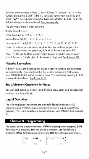
Chapter 8 : Programming
The options on the program menu are: NEW (for creating a new program), RUN (for executing a program), EDIT (for editing a program), DEL (for deleting a program), TRACE (for tracing a program), and EXIT (for exiting program mode).
E-26
Before Using the Program Area
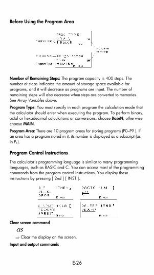
Number of Remaining Steps: The program capacity is 400 steps. The number of steps indicates the amount of storage space available for programs, and it will decrease as programs are input. The number of remaining steps will also decrease when steps are converted to memories. See Array Variables above.
Program Type: You must specify in each program the calculation mode that the calculator should enter when executing the program. To perform binary, octal or hexadecimal calculations or conversions, choose BaseN; otherwise choose MAIN.
Program Area: There are 10 program areas for storing programs (P0–P9 ). If an area has a program stored in it, its number is displayed as a subscript (as in P1).
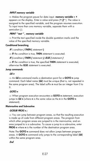
Program Control Instructions
The calculator’s programming language is similar to many programming languages, such as BASIC and C. You can access most of the programming commands from the program control instructions. You display these instructions by pressing [ 2nd ] [ INST ].
Clear screen command
CLS
⇒ Clear the display on the screen.
Input and output commands
E-27
INPUT memory variable
⇒ Makes the program pause for data input. memory variable = appears on the display. Enter a value and press [ ]. The value is assigned to the specified variable, and the program resumes execution. To input more than one memory variable, separate them with a semicolon (;).
PRINT “ text ” , memory variable
⇒ Print the text specified inside the double quotation marks and the value of the specified memory variable.
Conditional branching
IF ( condition ) THEN { statement }
⇒ IF the condition is true, THEN statement is executed.
IF ( condition ) THEN { statement }; ELSE { statement }
⇒ IF the condition is true, the specified THEN statement is executed, otherwise the ELSE statement is executed.
Jump commands
Lbl n
⇒ An Lbl n command marks a destination point for a GOTO n jump command. Each label name (Lbl) must be unique (that is, not repeated in the same program area). The label suffix n must be an integer from 0 to 9.
GOTO n
⇒ When program execution encounters a GOTO n statement, execution jumps to Lbl n (where n is the same value as the n in the GOTO n statement).
Mainroutine and Subroutine
GOSUB PROG n ;
⇒ You can jump between program areas, so that the resulting execution is made up of code from different program areas. The program from which other program areas are jumped to is the mainroutine, and an area jumped to is a subroutine. To cause a jump to a subroutine, enter PROG n where n is the number of the destination program area.
Note: The GOTO n command does not allow jumps between program areas. A GOTO n command only jumps to the corresponding label (Lbl) within the same program area.
End
E-28
⇒ Each program needs an END command to mark the end of the program. This is displayed automatically when you create a new program.
Increment and decrement
Post-fixed: Memory variable + + or Memory variable – –
Pre-fixed: + + Memory variable or – – Memory variable
⇒ A memory variable is decreased or increased by one. For standard memory variables, the + + ( Increment ) and – – ( Decrement ) operators can be either post-fixed or pre-fixed. For array variables, the operators must be pre-fixed.
With pre-fixed operators, the memory variable is computed before the expression is evaluated; with post-fixed operators, the memory variable is computed after the expression is evaluated.
For loop
FOR ( start condition; continue condition; re-evaluation ) { statements }
⇒ A FOR loop is useful for repeating a set of similar actions while a specified counter is between certain values.
For example:
FOR ( A = 1 ; A ≤ 4 ; A + + )
{ C = 3 × A ; PRINT ” ANS = ” , C }
END
⇒ Result : ANS = 3, ANS = 6, ANS = 9, ANS = 12
The processing in this example is: 1. FOR A = 1: This initializes the value of A to 1. Since A = 1 is consistent
with A ≤ 4, the statements are executed and A is incremented by 1. 2. Now A = 2. This is consistent with A ≤ 4, so the statements are
executed and A is again incremented by 1. And so on. 3. When A = 5, it is no longer true that A ≤ 4, so statements are not
executed. The program then moves on to the next block of code. Sleep command
SLEEP ( time )
⇒ A SLEEP command suspends program execution for a specified time (up to a maximum of 105 seconds). This is useful for displaying intermediate results before resuming execution.
Swap command
SWAP ( memory variable A, memory variable B )
E-29
⇒ The SWAP command swaps the contents in two memory variables.
Relational Operators
The relational operators that can be used in FOR loops and conditional branching are:
= = (equal to), < (less than), > (greater than), ≠ (not equal to), ≤ (less than or equal to), ≥ (greater than or equal to).
Creating a New Program
1. Select NEW from the program menu and press [ ]. 2. Select the calculation mode you want the program to run in and press
[ ]. 3. Select one of the ten program areas (P0123456789) and press [ ]. 4. Enter your program’s commands.
• You can enter the calculator’s regular functions as commands. • To enter a program control instruction, press [ 2nd ] [ INST ] and make your selection. • To enter a space, press [ ALPHA ] [ SPC ].
5. A semicolon (;) indicates the end of a command. To enter more than one command on a command line, separate them with a semicolon. For example: Line 1: INPUT A ; C = 0.5 × A ; PRINT ” C = ” , C ; END You can also place each command or group of commands on a separate line, as follows. In this case, a trailing semicolon can be omitted. Line 1: INPUT A ; C = 0.5 × A [ ] Line 2: PRINT ” C = ” , C ; END
Executing a Program
1. When you finish entering or editing a program, press [ CL/ESC ] to return to the program menu, select RUN and press [ ]. (Or you can press [ PROG ] in MAIN mode.)
2. Select the relevant program area and press [ ] to begin executing the program.
3. To re-execute the program, press [ ] while the program’s final result is on the display.
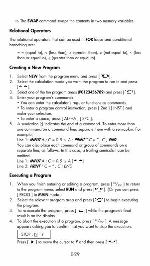
4. To abort the execution of a program, press [ CL/ESC ]. A message appears asking you to confirm that you want to stop the execution.
STOP : N Y
Press [ ] to move the cursor to Y and then press [ ].
E-30
Debugging a Program
A program might generate an error message or unexpected results when it is executed. This indicates that there is an error in the program that needs to be corrected.
• Error messages appear for approximately 5 seconds, and then the cursor blinks at the location of the error.
• To correct an error, select EDIT from the program menu.
• You also can select TRACE from the program menu. The program is then checked step-by-step and a message alerts you to any errors.
Using the Graph Function in Programs
Using the graph function within programs enables you to graphically illustrate long or complex equations and to overwrite graphs repeatedly. All graph commands (except trace and zoom) can be included in programs. Range values can also be specified in the program.
Note that values in some graph commands must be separated by commas (,) as follows:
• Range ( Xmin, Xmax, Xscl, Ymin, Ymax, Yscl )
• Factor ( Xfact, Yfact )
• Plot ( X point, Y point )
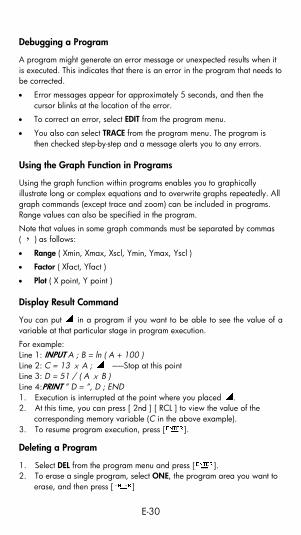
Display Result Command
You can put in a program if you want to be able to see the value of a variable at that particular stage in program execution.
For example: Line 1: INPUT A ; B = ln ( A + 100 ) Line 2: C = 13 × A ; -------Stop at this point Line 3: D = 51 / ( A × B ) Line 4:PRINT ” D = ”, D ; END 1. Execution is interrupted at the point where you placed . 2. At this time, you can press [ 2nd ] [ RCL ] to view the value of the
corresponding memory variable (C in the above example). 3. To resume program execution, press [ ].
Deleting a Program
1. Select DEL from the program menu and press [ ]. 2. To erase a single program, select ONE, the program area you want to
erase, and then press [ ]

E-31
3. To erase all the programs, select ALL. 4. A message appears asking you to confirm that you want to delete the
program(s).
Press [ ] to move the cursor to Y and then press [ ]. 5. To exit DEL mode, select EXIT from the program menu.
Program Examples
See Examples 54 to 63.
Example 1 Change 123 × 45 to 123 × 475
123 [ × ] 45 [ ]
[ ] [ ] [ ] [ DEL ]
[ 2nd ] [ ]
[ ] [ ] 7 [ ]
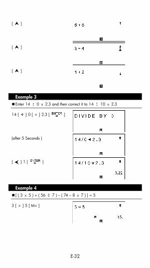
Example 2 After executing 1 + 2, 3 + 4, 5 + 6, recall each expression
1 [ + ] 2 [ ] 3 [ + ] 4 [ ] 5 [ + ] 6 [ ]
E-32
[ ]
[ ]
[ ]
Example 3 Enter 14 0 × 2.3 and then correct it to 14 10 × 2.3
14 [ ] 0 [ × ] 2.3 [ ]
(after 5 Seconds )
[ ] 1 [ ]
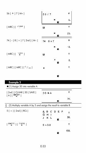
Example 4 [ ( 3 × 5 ) + ( 56 7 ) – ( 74 – 8 × 7 ) ] = 5
3 [ × ] 5 [ M+ ]
E-33
56 [ ] 7 [ M+ ]
[ MRC ] [ ]
74 [ – ] 8 [ × ] 7 [ 2nd ] [ M– ]
[ MRC ] [ ]
[ MRC ] [ MRC ] [ CL / ESC ]
Example 5 (1) Assign 30 into variable A
[ 2nd ] [ CL-VAR ] 30 [ SAVE ] [ A ] [ ]
0 (2) Multiply variable A by 5 and assign the result to variable B
5 [ × ] [ 2nd ] [ RCL ]
[ ] [ ]
E-34
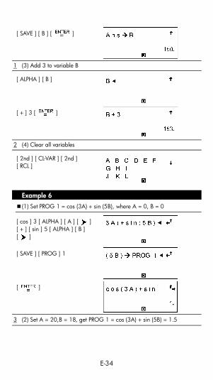
[ SAVE ] [ B ] [ ]
1 (3) Add 3 to variable B
[ ALPHA ] [ B ]
[ + ] 3 [ ]
2 (4) Clear all variables
[ 2nd ] [ CL-VAR ] [ 2nd ] [ RCL ]
Example 6 (1) Set PROG 1 = cos (3A) + sin (5B), where A = 0, B = 0
[ cos ] 3 [ ALPHA ] [ A ] [ ] [ + ] [ sin ] 5 [ ALPHA ] [ B ] [ ]
[ SAVE ] [ PROG ] 1
[ ]
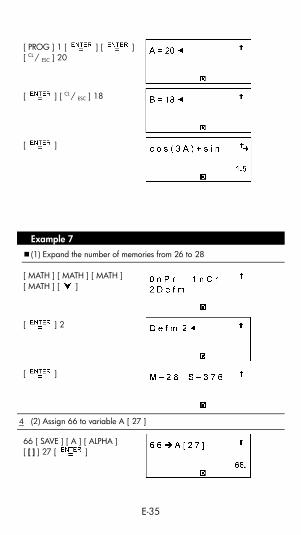
3 (2) Set A = 20,B = 18, get PROG 1 = cos (3A) + sin (5B) = 1.5
E-35
[ PROG ] 1 [ ] [ ] [ CL / ESC ] 20
[ ] [ CL / ESC ] 18
[ ]
Example 7 (1) Expand the number of memories from 26 to 28
[ MATH ] [ MATH ] [ MATH ] [ MATH ] [ ]
[ ] 2
[ ]
4 (2) Assign 66 to variable A [ 27 ]
66 [ SAVE ] [ A ] [ ALPHA ] [ [ ] ] 27 [ ]

E-36
5 (3) Recall variable A [ 27 ]
[ ALPHA ] [ A ] [ ALPHA ] [ [ ] ] 27 [ ]
6 (4) Return memory variables to the default configuration
[ MATH ] [ MATH ] [ MATH ] [ MATH ] [ ]
[ ] 0 [ ]
Example 8 7 + 10 × 8 2 = 47
7 [ + ] 10 [ × ] 8 [ ] 2 [ ]
Example 9 – 3.5 + 8 4 = –1.5
[ ( – ) ] 3.5 [ + ] 8 [ ] 4 [ ]
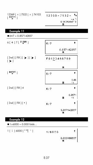
Example 10 12369 × 7532 × 74103 = 6903680613000
E-37
12369 [ × ] 7532 [ × ] 74103 [ ]
Example 11 6 7 = 0.857142857
6 [ ] 7 [ ]
[ 2nd ] [ FIX ] [ ] [ ] [ ]
[ ]
[ 2nd ] [ FIX ] 4
[ 2nd ] [ FIX ] [ • ]
Example 12 1 6000 = 0.0001666...
1 [ ] 6000 [ ]
E-38
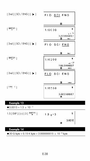
[ 2nd ] [ SCI / ENG ] [ ]
[ ]
[ 2nd ] [ SCI / ENG ] [ ]
[ ]
[ 2nd ] [ SCI / ENG ] [ ]
[ ]
Example 13 0.0015 = 1.5 × 10 – 3
1.5 [ EXP ] [ (–) ] 3 [ ]
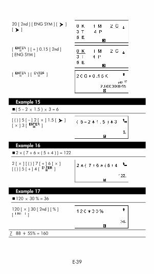
Example 14 20 G byte + 0.15 K byte = 2.000000015 × 10 10 byte
E-39
20 [ 2nd ] [ ENG SYM ] [ ] [ ]
[ ] [ + ] 0.15 [ 2nd ] [ ENG SYM ]
[ ] [ ]
Example 15 ( 5 – 2 × 1.5 ) × 3 = 6
[ ( ) ] 5 [ – ] 2 [ × ] 1.5 [ ] [ × ] 3 [ ]
Example 16 2 × { 7 + 6 × ( 5 + 4 ) } = 122
2 [ × ] [ ( ) ] 7 [ + ] 6 [ × ] [ ( ) ] 5 [ + ] 4 [ ]
Example 17 120 × 30 % = 36
120 [ × ] 30 [ 2nd ] [ % ] [ ]
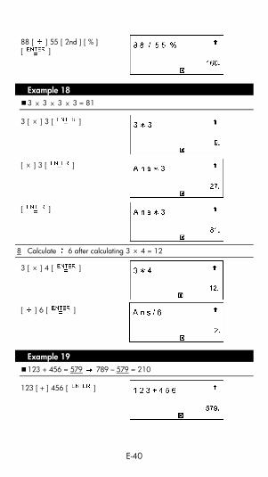
7 88 55% = 160
E-40
88 [ ] 55 [ 2nd ] [ % ] [ ]
Example 18 3 × 3 × 3 × 3 = 81
3 [ × ] 3 [ ]
[ × ] 3 [ ]
[ ]
8 Calculate 6 after calculating 3 × 4 = 12
3 [ × ] 4 [ ]
[ ] 6 [ ]
Example 19 123 + 456 = 579 789 – 579 = 210
123 [ + ] 456 [ ]
E-41
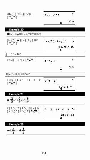
789 [ – ] [ 2nd ] [ ANS ] [ ]
Example 20 ln7 + log100 = 3.945910149
[ ln ] 7 [ ] [ + ] [ log ] 100 [ ]
9 10 2 = 100
[ 2nd ] [ 10 x ] 2 [ ]
10 e –5 = 0.006737947
[ 2nd ] [ e x ] [ ( – ) ] 5 [ ]
Example 21
7 [ A b/c ] 2 [ A b/c ] 3 [ + ] 14 [ A b/c ] 5 [ A b/c ] 7 [ ]
Example 22
E-42
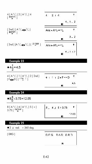
4 [ A b/c ] 2 [ A b/c ] 4 [ ]
[ 2nd ] [ A b/cd/e ]
[ ]
[ 2nd ] [A b/cd/e ] [ ]
Example 23
4 [ A b/c ] 1 [ A b/c ] 2 [ 2nd ] [ F D ] [ ]
Example 24
8 [ A b/c ] 4 [ A b/c ] 5 [ + ] 3.75 [ ]
Example 25 2 rad. = 360 deg.
[ DRG ]
E-43
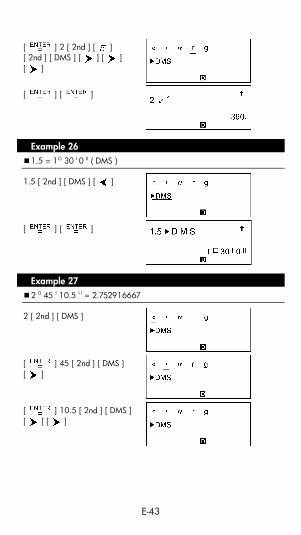
[ ] 2 [ 2nd ] [ ] [ 2nd ] [ DMS ] [ ] [ ] [ ]
[ ] [ ]
Example 26 1.5 = 1O 30 I 0 II ( DMS )
1.5 [ 2nd ] [ DMS ] [ ]
[ ] [ ]
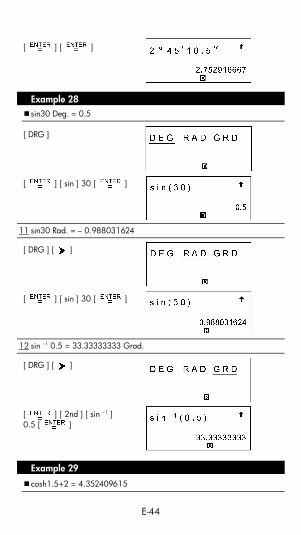
Example 27 2 0 45 I 10.5 I I = 2.752916667
2 [ 2nd ] [ DMS ]
[ ] 45 [ 2nd ] [ DMS ] [ ]
[ ] 10.5 [ 2nd ] [ DMS ] [ ] [ ]
E-44
[ ] [ ]
Example 28 sin30 Deg. = 0.5
[ DRG ]
[ ] [ sin ] 30 [ ]
11 sin30 Rad. = – 0.988031624
[ DRG ] [ ]
[ ] [ sin ] 30 [ ]
12 sin –1 0.5 = 33.33333333 Grad.
[ DRG ] [ ]
[ ] [ 2nd ] [ sin –1 ] 0.5 [ ]
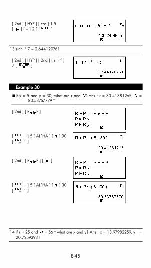
Example 29 cosh1.5+2 = 4.352409615
E-45
[ 2nd ] [ HYP ] [ cos ] 1.5 [ ] [ + ] 2 [ ]
13 sinh –1 7 = 2.644120761
[ 2nd ] [ HYP ] [ 2nd ] [ sin –1 ] 7 [ ]
Example 30
If x = 5 and y = 30, what are r and ? Ans : r = 30.41381265, = 80.53767779 o
[ 2nd ] [ R P ]
[ ] 5 [ ALPHA ] [ ] 30 [ ]
[ 2nd ] [ R P ] [ ]
[ ] 5 [ ALPHA ] [ ] 30 [ ]
14 If r = 25 and = 56 o what are x and y? Ans : x = 13.97982259, y = 20.72593931
E-46
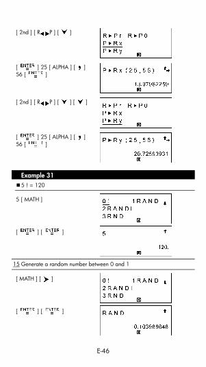
[ 2nd ] [ R P ] [ ]
[ ] 25 [ ALPHA ] [ ] 56 [ ]
[ 2nd ] [ R P ] [ ] [ ]
[ ] 25 [ ALPHA ] [ ] 56 [ ]
Example 31 5 ! = 120
5 [ MATH ]
[ ] [ ]
15 Generate a random number between 0 and 1
[ MATH ] [ ]
[ ] [ ]
E-47
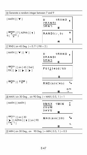
16 Generate a random integer between 7 and 9
[ MATH ] [ ]
[ ] 7 [ ALPHA ] [ ] 9 [ ]
17 RND ( sin 45 Deg. ) = 0.71 ( FIX = 2 )
[ MATH ] [ ] [ ]
[ ] [ sin ] 45 [ 2nd ] [ FIX ] [ ] [ ] [ ]
[ ] [ ]
18 MAX ( sin 30 Deg. , sin 90 Deg. ) = MAX ( 0.5, 1 ) = 1
[ MATH ] [ MATH ]
[ ] [ sin ] 30 [ ] [ ALPHA ] [ ] [ sin ] 90 [ ]
19 MIN ( sin 30 Deg., sin 90 Deg. ) = MIN ( 0.5, 1 ) = 0.5
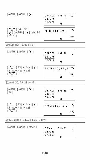
E-48
[ MATH ] [ MATH ] [ ]
[ ] [ sin ] 30 [ ] [ ALPHA ] [ ] [ sin ] 90 [ ]
20 SUM (13, 15, 23 ) = 51
[ MATH ] [ MATH ] [ ]
[ ] 13 [ ALPHA ] [ ] 15 [ ALPHA ] [ ] 23 [ ]
21 AVG (13, 15, 23 ) = 17
[ MATH ] [ MATH ] [ ] [ ]
[ ] 13 [ ALPHA ] [ ] 15 [ ALPHA ] [ ] 23 [ ]
22 Frac (10 8 ) = Frac ( 1.25 ) = 0.25
[ MATH ] [ MATH ] [ MATH ]

E-49
[ ] 10 [ ] 8 [ ]
23 INT (10 8 ) = INT ( 1.25 ) = 1
[ MATH ] [ MATH ] [ MATH ] [ ]
[ ] 10 [ ] 8 [ ]
24 SGN ( log 0.01 ) = SGN ( – 2 ) = – 1
[ MATH ] [ MATH ] [ MATH ] [ ]
[ ] [ log ] 0.01 [ ]
25 ABS ( log 0.01) = ABS ( – 2 ) = 2
[ MATH ] [ MATH ] [ MATH ] [ ] [ ]
[ ] [ log ] 0.01 [ ]
E-50
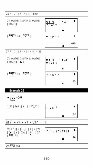
26 7 ! [ ( 7 – 4 ) ! ] = 840
7 [ MATH ] [ MATH ] [ MATH ] [ MATH ]
[ ] 4 [ ]
27 7 ! [ ( 7 – 4 ) ! × 4 ] = 35
7 [ MATH ] [ MATH ] [ MATH ] [ MATH ] [ ]
[ ] 4 [ ]
Example 32
1.25 [ 2nd ] [ X –1 ] [ ]
28
2 [ X 2 ] [ + ] [ ] 4 [ + ] 21 [ ] [ + ] [ 2nd ] [ ] 27 [ ]
29
E-51
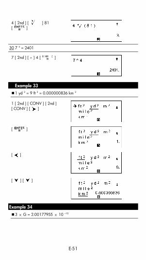
4 [ 2nd ] [ ] 81 [ ]
30 7 4 = 2401
7 [ 2nd ] [ ^ ] 4 [ ]
Example 33 1 yd 2 = 9 ft 2 = 0.000000836 km 2
1 [ 2nd ] [ CONV ] [ 2nd ] [ CONV ] [ ]
[ ]
[ ]
[ ] [ ]
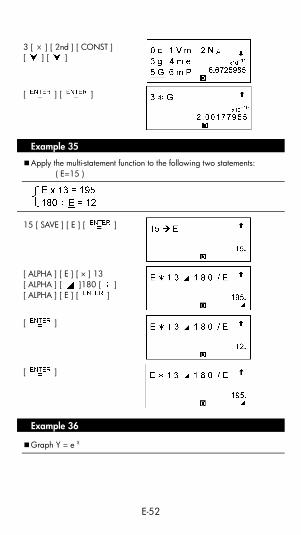
Example 34 3 × G = 2.00177955 × 10 –10
E-52
3 [ × ] [ 2nd ] [ CONST ] [ ] [ ]
[ ] [ ]
Example 35
Apply the multi-statement function to the following two statements: ( E=15 )
15 [ SAVE ] [ E ] [ ]
[ ALPHA ] [ E ] [ × ] 13 [ ALPHA ] [ ]180 [ ] [ ALPHA ] [ E ] [ ]
[ ]
[ ]
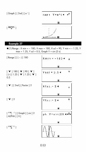
Example 36
Graph Y = e X
E-53
[ Graph ] [ 2nd ] [ e x ]
[ ]
Example 37
(1) Range : X min = – 180, X max = 180, X scl = 90, Y min = – 1.25, Y max = 1.25, Y scl = 0.5, Graph Y = sin (2 x)
[ Range ] [ ( – ) ] 180
[ ] 180 [ ] 90 [ ] [ (–) ] 1.25 [ ] 1.25 [ ] 0.5
[ ] [ 2nd ] [ Factor ] 2
[ ] 2
[ ] [ Graph ] [ sin ] 2 [ ALPHA ] [ X ]
[ ]
E-54
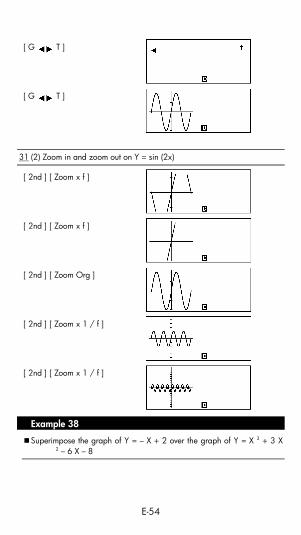
[ G T ]
[ G T ]
31 (2) Zoom in and zoom out on Y = sin (2x)
[ 2nd ] [ Zoom x f ]
[ 2nd ] [ Zoom x f ]
[ 2nd ] [ Zoom Org ]
[ 2nd ] [ Zoom x 1 / f ]
[ 2nd ] [ Zoom x 1 / f ]
Example 38
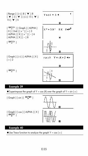
Superimpose the graph of Y = – X + 2 over the graph of Y = X 3 + 3 X 2 – 6 X – 8
E-55
[ Range ] [ (–) ] 8 [ ] 8 [ ] 2 [ ] [ (–) ] 15 [ ] 15 [ ] 5
[ ] [ Graph ] [ ALPHA ] [ X ] [ 2nd ] [ x 3 ] [ + ] 3 [ ALPHA ] [ X ] [ x 2 ] [ – ] 6 [ ALPHA ] [ X ] [ – ] 8
[ ]
[ Graph ] [ (–) ] [ ALPHA ] [ X ] [ + ] 2
[ ]
Example 39
Superimpose the graph of Y = cos (X) over the graph of Y = sin ( x )
[ Graph ] [ sin ] [ ]
[ Graph ] [ cos ] [ ALPHA ] [ X ] [ ]
Example 40
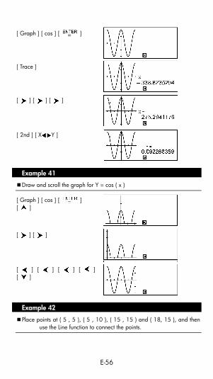
Use Trace function to analyze the graph Y = cos ( x )
E-56
[ Graph ] [ cos ] [ ]
[ Trace ]
[ ] [ ] [ ]
[ 2nd ] [ X Y ]
Example 41
Draw and scroll the graph for Y = cos ( x )
[ Graph ] [ cos ] [ ] [ ]
[ ] [ ]
[ ] [ ] [ ] [ ] [ ]
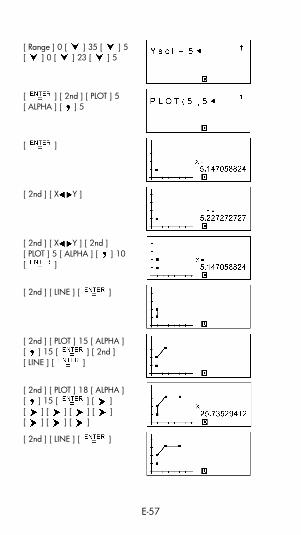
Example 42
Place points at ( 5 , 5 ), ( 5 , 10 ), ( 15 , 15 ) and ( 18, 15 ), and then use the Line function to connect the points.
E-57
[ Range ] 0 [ ] 35 [ ] 5 [ ] 0 [ ] 23 [ ] 5
[ ] [ 2nd ] [ PLOT ] 5 [ ALPHA ] [ ] 5
[ ]
[ 2nd ] [ X Y ]
[ 2nd ] [ X Y ] [ 2nd ] [ PLOT ] 5 [ ALPHA ] [ ] 10 [ ]
[ 2nd ] [ LINE ] [ ]
[ 2nd ] [ PLOT ] 15 [ ALPHA ] [ ] 15 [ ] [ 2nd ] [ LINE ] [ ]
[ 2nd ] [ PLOT ] 18 [ ALPHA ] [ ] 15 [ ] [ ] [ ] [ ] [ ] [ ] [ ] [ ] [ ]
[ 2nd ] [ LINE ] [ ]
E-58
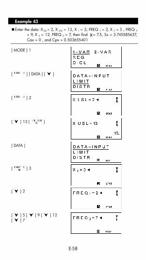
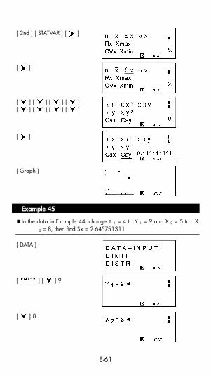
Example 43
Enter the data: X LSL = 2, X USL = 13, X 1 = 3, FREQ 1 = 2, X 2 = 5 , FREQ 2 = 9, X 3 = 12, FREQ 3 = 7, then find = 7.5, Sx = 3.745585637, Cax = 0 , and Cpx = 0.503655401
[ MODE ] 1
[ ] [ DATA ] [ ]
[ ] 2
[ ] 13 [ ]
[ DATA ]
[ ] 3
[ ] 2
[ ] 5 [ ] 9 [ ] 12 [ ] 7
E-59
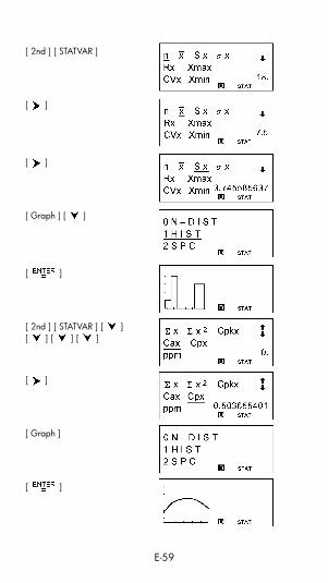
[ 2nd ] [ STATVAR ]
[ ]
[ ]
[ Graph ] [ ]
[ ]
[ 2nd ] [ STATVAR ] [ ] [ ] [ ] [ ]
[ ]
[ Graph ]
[ ]
E-60
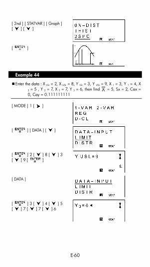
[ 2nd ] [ STATVAR ] [ Graph ] [ ] [ ]
[ ]
Example 44
Enter the data : X LSL = 2, X USL = 8, Y LSL = 3, Y USL = 9, X 1 = 3, Y 1 = 4, X 2 = 5 , Y 2 = 7, X 3 = 7, Y 3 = 6, then find = 5, Sx = 2, Cax = 0, Cay = 0.111111111
[ MODE ] 1 [ ]
[ ] [ DATA ] [ ]
[ ] 2 [ ] 8 [ ] 3 [ ] 9 [ ]
[ DATA ]
[ ] 3 [ ] 4 [ ] 5 [ ] 7 [ ] 7 [ ] 6
E-61
[ 2nd ] [ STATVAR ] [ ]
[ ]
[ ] [ ] [ ] [ ] [ ] [ ] [ ] [ ]
[ ]
[ Graph ]
Example 45
In the data in Example 44, change Y 1 = 4 to Y 1 = 9 and X 2 = 5 to X 2 = 8, then find Sx = 2.645751311
[ DATA ]
[ ] [ ] 9
[ ] 8
E-62
[ 2nd ] [ STATVAR ] [ ] [ ]
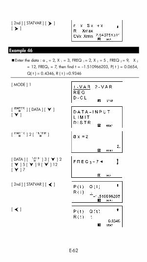
Example 46
Enter the data : a x = 2, X 1 = 3, FREQ 1 = 2, X 2 = 5 , FREQ 2 = 9, X 3
= 12, FREQ3 = 7, then find t = –1.510966203, P( t ) = 0.0654,
Q( t ) = 0.4346, R ( t ) =0.9346
[ MODE ] 1
[ ] [ DATA ] [ ] [ ]
[ ] 2 [ ]
[ DATA ] [ ] 3 [ ] 2 [ ] 5 [ ] 9 [ ] 12 [ ] 7
[ 2nd ] [ STATVAR ] [ ]
[ ]
E-63
[ ]
[ ]
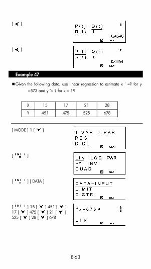
Example 47
Given the following data, use linear regression to estimate x ’ =? for y
=573 and y ’= ? for x = 19
X 15 17 21 28
Y 451 475 525 678
[ MODE ] 1 [ ]
[ ]
[ ] [ DATA ]
[ ] 15 [ ] 451 [ ] 17 [ ] 475 [ ] 21 [ ] 525 [ ] 28 [ ] 678
E-64
[ 2 nd ] [ STATVAR ] [ Graph ]
[ 2nd ] [ STATVAR ] [ ] [ ] [ ]
[ ] 573 [ ]
[ 2nd ] [ STATVAR ] [ ] [ ] [ ] [ ]
[ ] 19 [ ]
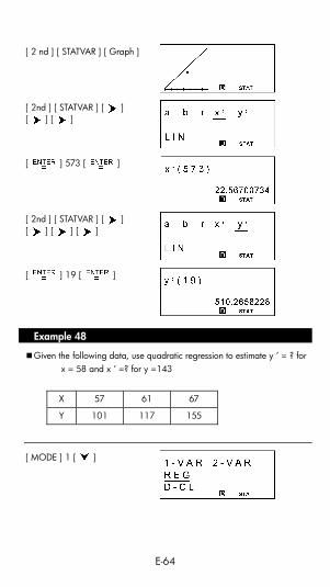
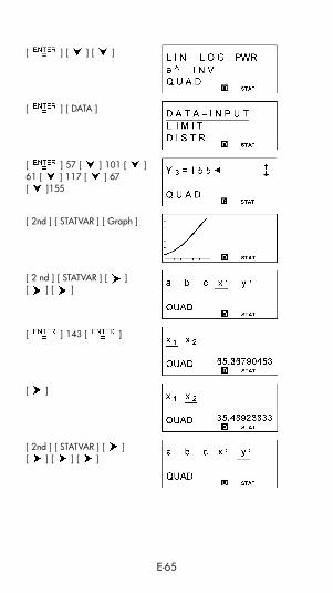
Example 48
Given the following data, use quadratic regression to estimate y ’ = ? for x = 58 and x ’ =? for y =143
X 57 61 67
Y 101 117 155
[ MODE ] 1 [ ]
E-65
[ ] [ ] [ ]
[ ] [ DATA ]
[ ] 57 [ ] 101 [ ] 61 [ ] 117 [ ] 67 [ ]155
[ 2nd ] [ STATVAR ] [ Graph ]
[ 2 nd ] [ STATVAR ] [ ] [ ] [ ]
[ ] 143 [ ]
[ ]
[ 2nd ] [ STATVAR ] [ ] [ ] [ ] [ ]
E-66
[ ] 58 [ ]
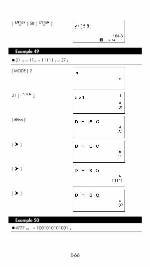
Example 49
31 10 = 1F16 = 11111 2 = 37 8
[ MODE ] 2
31 [ ]
[ dhbo ]
[ ]
[ ]
[ ]
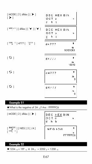
Example 50 4777 10 = 1001010101001 2
E-67
[ MODE ] 2 [ dhbo ] [ ] [ ]
[ ] [ dhbo ] [ ] [ ]
[ ] 4777 [ ]
[ ]
[ ]
[ ]
Example 51 What is the negative of 3A 16? Ans : FFFFFFC6
[ MODE ] 2 [ dhbo ] [ ]
[ ] [ NEG ] 3 [ /A ] [ ]
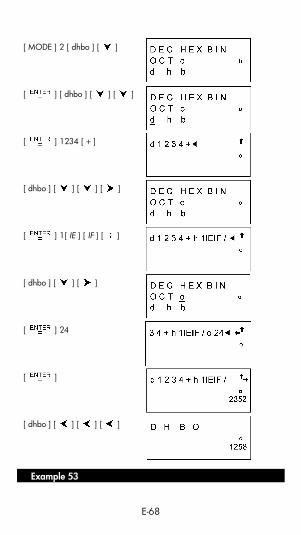
Example 52 1234 10 + 1EF 16 24 8 = 2352 8 = 1258 10
E-68
[ MODE ] 2 [ dhbo ] [ ]
[ ] [ dhbo ] [ ] [ ]
[ ] 1234 [ + ]
[ dhbo ] [ ] [ ] [ ]
[ ] 1[ IE ] [ IF ] [ ]
[ dhbo ] [ ] [ ]
[ ] 24
[ ]
[ dhbo ] [ ] [ ] [ ]
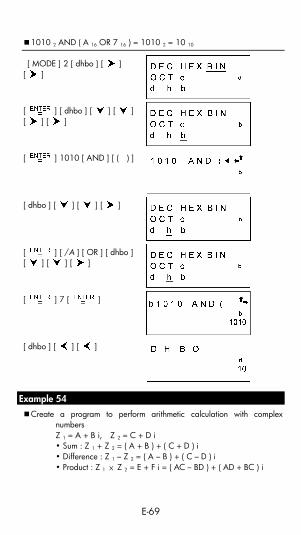
Example 53
E-69
1010 2 AND ( A 16 OR 7 16 ) = 1010 2 = 10 10
[ MODE ] 2 [ dhbo ] [ ] [ ]
[ ] [ dhbo ] [ ] [ ] [ ] [ ]
[ ] 1010 [ AND ] [ ( ) ]
[ dhbo ] [ ] [ ] [ ]
[ ] [ /A ] [ OR ] [ dhbo ] [ ] [ ] [ ]
[ ] 7 [ ]
[ dhbo ] [ ] [ ]
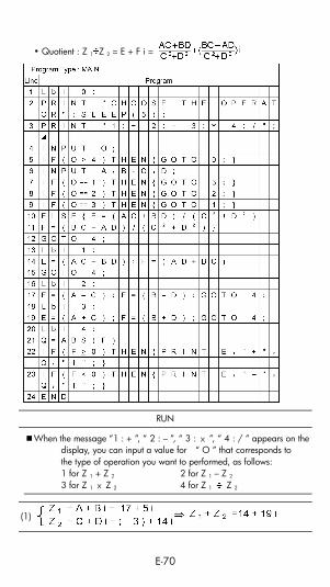
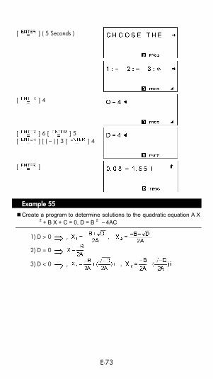
Example 54 Create a program to perform arithmetic calculation with complex
numbers Z 1 = A + B i, Z 2 = C + D i • Sum : Z 1 + Z 2 = ( A + B ) + ( C + D ) i • Difference : Z 1 – Z 2 = ( A – B ) + ( C – D ) i • Product : Z 1 × Z 2 = E + F i = ( AC – BD ) + ( AD + BC ) i
E-70
• Quotient : Z 1 Z 2 = E + F i =
RUN
When the message “1 : + ”, “ 2 : – ”, “ 3 : × ”, “ 4 : / ” appears on the display, you can input a value for “ O ” that corresponds to the type of operation you want to performed, as follows: 1 for Z 1 + Z 2 2 for Z 1 – Z 2 3 for Z 1 × Z 2 4 for Z 1 Z 2
(1)
E-71
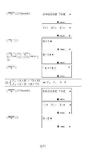
[ ] ( 5 Seconds )
[ ] 1
[ ] 17 [ ] 5 [ ] [ ( – ) ] 3 [ ] 14
[ ]
(2)
[ ] ( 5 Seconds )
[ ] 2
E-72
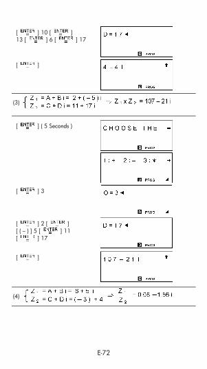
[ ] 10 [ ] 13 [ ] 6 [ ] 17
[ ]
(3)
[ ] ( 5 Seconds )
[ ] 3
[ ] 2 [ ] [ ( – ) ] 5 [ ] 11 [ ] 17
[ ]
(4)
E-73
[ ] ( 5 Seconds )
[ ] 4
[ ] 6 [ ] 5 [ ] [ ( – ) ] 3 [ ] 4
[ ]
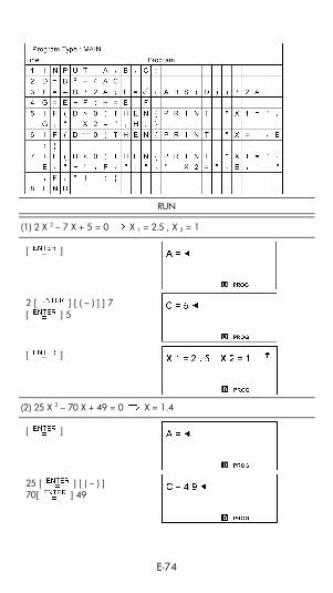
Example 55 Create a program to determine solutions to the quadratic equation A X
2 + B X + C = 0, D = B 2 – 4AC
1) D > 0 , ,
2) D = 0
3) D < 0 , ,
E-74
RUN
(1) 2 X 2 – 7 X + 5 = 0 X 1 = 2.5 , X 2 = 1
[ ]
2 [ ] [ ( – ) ] ] 7 [ ] 5
[ ]
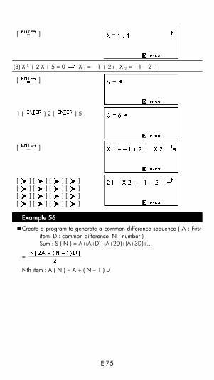
(2) 25 X 2 – 70 X + 49 = 0 X = 1.4
[ ]
25 [ ] [ ( – ) ] 70[ ] 49
E-75
[ ]
(3) X 2 + 2 X + 5 = 0 X 1 = – 1 + 2 i , X 2 = – 1 – 2 i
[ ]
1 [ ] 2 [ ] 5
[ ]
[ ] [ ] [ ] [ ] [ ] [ ] [ ] [ ] [ ] [ ] [ ] [ ] [ ] [ ] [ ] [ ]
Example 56 Create a program to generate a common difference sequence ( A : First
item, D : common difference, N : number ) Sum : S ( N ) = A+(A+D)+(A+2D)+(A+3D)+...
=
Nth item : A ( N ) = A + ( N – 1 ) D
E-76
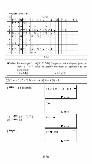
RUN
When the message “ 1: A(N), 2 :S(N) ” appears on the display, you can input a “ P ” value to specify the type of operation to be performed: 1 for A(N) 2 for S(N)
32 (1) A = 3 , D = 2, N = 4 A(N) = A (4) = 9
[ ] ( 5 Seconds )
1 [ ] 3 [ ] 2 [ ] 4
[ ]
E-77
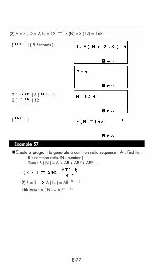
(2) A = 3 , D = 2, N = 12 S (N) = S (12) = 168
[ ] ( 5 Seconds )
2 [ ] 3 [ ] 2 [ ] 12
[ ]
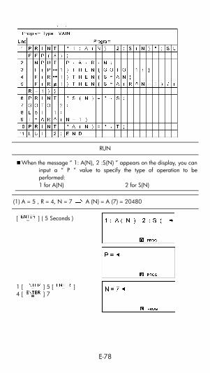
Example 57 Create a program to generate a common ratio sequence ( A : First item,
R : common ratio, N : number ) Sum : S ( N ) = A + AR + AR 2 + AR3....
1) R 1
2) R = 1 A ( N ) = AR ( N – 1 )
Nth item : A ( N ) = A ( N – 1 )
E-78
RUN
When the message “ 1: A(N), 2 :S(N) ” appears on the display, you can input a “ P ” value to specify the type of operation to be performed: 1 for A(N) 2 for S(N)
(1) A = 5 , R = 4, N = 7 A (N) = A (7) = 20480
[ ] ( 5 Seconds )
1 [ ] 5 [ ] 4 [ ] 7
E-79
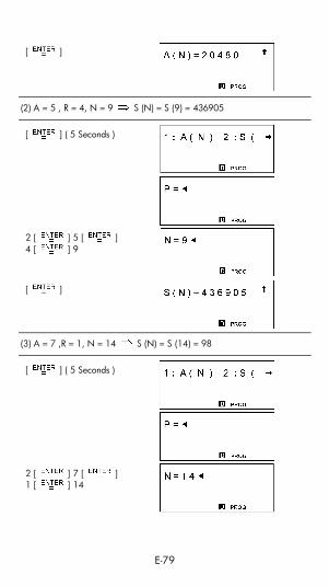
[ ]
(2) A = 5 , R = 4, N = 9 S (N) = S (9) = 436905
[ ] ( 5 Seconds )
2 [ ] 5 [ ] 4 [ ] 9
[ ]
(3) A = 7 ,R = 1, N = 14 S (N) = S (14) = 98
[ ] ( 5 Seconds )
2 [ ] 7 [ ] 1 [ ] 14
E-80
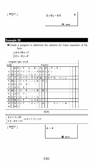
[ ]
Example 58 Create a program to determine the solutions for linear equations of the
form:
RUN
[ ]

E-81
4
[ ] [ ( – ) ] 1 [ ] 30 [ ] 5 [ ] 9 [ ] 17
[ ]
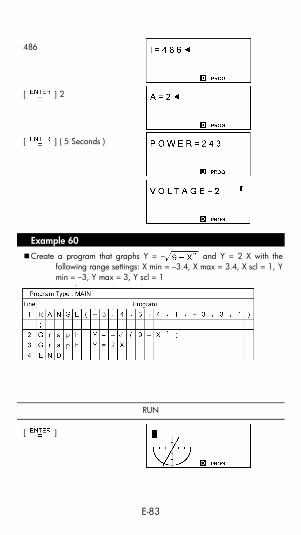
Example 59
Create three subroutines to store the following formulas and then use the GOSUB-PROG command to write a mainroutine to execute the subroutines. Subroutine 1 : CHARGE = N × 3 Subroutine 2 : POWER = I A Subroutine 3 : VOLTAGE = I ( B × Q × A )

E-82
RUN
N = 1.5, I = 486, A = 2 CHARGE = 4.5, POWER = 243, VOLTAGE = 2
[ ]
1.5
[ ] ( 5 Seconds )
E-83
486
[ ] 2
[ ] ( 5 Seconds )
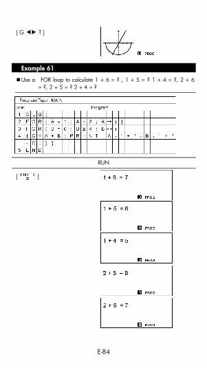
Example 60 Create a program that graphs Y = – and Y = 2 X with the
following range settings: X min = –3.4, X max = 3.4, X scl = 1, Y min = –3, Y max = 3, Y scl = 1
RUN
[ ]
E-84
[ G T ]
Example 61
Use a FOR loop to calculate 1 + 6 = ? , 1 + 5 = ? 1 + 4 = ?, 2 + 6 = ?, 2 + 5 = ? 2 + 4 = ?
RUN
[ ]

E-85
Example 62 Set the program type to “BaseN” and evaluate
ANS = 1010 2 AND ( Y OR 7 16 )
(1) If Y = /A 16 , Ans = 10 10
[ ]
[ dhbo ] [ ] [ ] [ ]
[ ] / A
[ ]
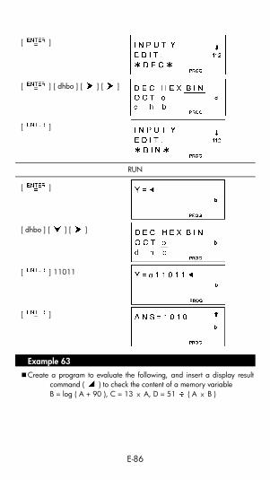
(2) If Y =11011 8 , Ans = 1010 2
EDIT
E-86
[ ]
[ ] [ dhbo ] [ ] [ ]
[ ]
RUN
[ ]
[ dhbo ] [ ] [ ]
[ ] 11011
[ ]
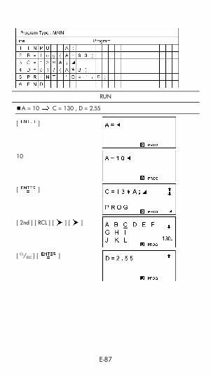
Example 63 Create a program to evaluate the following, and insert a display result
command ( ) to check the content of a memory variable B = log ( A + 90 ), C = 13 × A, D = 51 ( A × B )
E-87
RUN
A = 10 C = 130 , D = 2.55
[ ]
10
[ ]
[ 2nd ] [ RCL ] [ ] [ ]
[ CL/ESC ] [ ]