hp boundary element modeling of the external human auditory system––goal-oriented adaptivity...

hp Boundary element modeling of the external humanauditory system––goal-oriented adaptivity with

multiple load vectors

Timothy Walsh, Leszek Demkowicz *

Texas Institute for Computational and Applied Mathematics, The University of Texas at Austin, SHC 304,

Campus Code C0200 105 W. 26th Street, ACES 6.332, Austin, TX 78712, USA

Received 5 February 2001

Abstract

In this paper we consider two common problems encountered in boundary element analysis of acoustical scattering

problems. The first is the need to resolve the solution only in a finite subregion of the domain, instead of resolving the

solution in a global energy norm. This could occur, for example, when attempting to match experimental data that

involved microphones placed at discrete points of the domain. The second unresolved issue is multiple right-hand sides,

which correspond to rotating angles of incidence of an impinging plane or spherical wave. Constructing a separate

adaptive mesh for each right-hand side would quickly become impractical. In this work we present a goal-oriented

adaptivity procedure for resolving the boundary element solution only in a finite subregion of the domain, and we

implement the method within a multiple right-hand sides context, so that the resulting meshes will be optimized not

only for the selected subdomain, but also for all right-hand sides simultaneously. All of this work is part of a general

effort to model the external human auditory system. More extensive results on using the above methodology for

computing the head-related transfer function of a typical human head/ear will be presented in a forthcoming publi-

cation.

� 2002 Elsevier Science B.V. All rights reserved.

Keywords: hp Boundary element method; HRTF; External ear; Geometry reconstruction; Goal-oriented adaptivity

1. Introduction

1.1. Motivation

Adaptive refinement is a critical feature of the boundary element method, even more so than in the finite

element method. In the case of boundary elements, every degree of freedom that is omitted by using localrefinement rather than uniform refinement eliminates a row and column of a dense matrix. This eliminates

*Corresponding author. Tel.: +1-512-471-3312; fax: +1-512-471-8694.

E-mail address: [email protected] (L. Demkowicz).

0045-7825/03/$ - see front matter � 2002 Elsevier Science B.V. All rights reserved.

PII: S0045-7825 (02 )00536-4

Comput. Methods Appl. Mech. Engrg. 192 (2003) 125–146

www.elsevier.com/locate/cma

mail to: [email protected]

the need for storing the row and column, as well as the extra work involved in forming and factorizing thelinear system. By comparison, the finite element method usually produces only a banded matrix, and so in

this case adaptive refinement will have a less dramatic reduction on the tasks of matrix storage, formation,

and factorization. And yet, the literature on adaptive finite element methods is much more extensive than

in the case of boundary element methods. In particular, the quantity of interest or goal-oriented error esti-

mation and mesh refinement techniques, which have recently been introduced into the finite element

method, have not been applied to boundary element techniques. In this paper we will present an imple-

mentation of the goal-oriented error estimation technique within the context of the boundary element

method for the Helmholtz integral equation.The head-related transfer function (HRTF), used by acousticians and audiologists in understanding

the localization process, as well as in the design of hearing aids, virtual acoustic simulators, and in tests

for hearing system damage, is normally measured using a rotating frame in an anechoic chamber.

This procedure is time consuming and expensive, and does not allow for parametric studies of the effects

of various geometrical features on the overall response. Numerical simulations of the HRTF provide

the advantage that parametric studies can be performed simply by changing the input parameters to the

code.

However, simulations of this type present two immediate challenges to the numerical analyst, both ofwhich are common to most acoustical scattering applications. The first is that the microphone measuring

the pressure is placed only at the eardrum of the subject, and thus an adaptive refinement strategy is needed

that accelerates the convergence of the pressure in this small subregion of the domain. In this case, classical

refinement strategies based on global energy norms are not the optimal choice. Second, from the appli-

cation standpoint the goal is not so much to compute the solution due to a single source location, but to

compute the response as a function of the source location. One approach would be to divide the angular 360�space into several increments, and compute the corresponding pressure solution for each source location.

However, even with a goal-oriented adaptive approach, one would have to compute a separate adaptivemesh for each source location, and this would quickly become impractical.

This motivates the following two algorithms for consideration in this paper:

• A goal-oriented adaptivity procedure for boundary element methods to allow for resolving the acoustic

pressure only in a selected subregion of the domain, rather than in a global energy norm.

• An adaptivity procedure for the case of multiple right-hand sides, to allow for generation of a single hpmesh which is optimized for all right-hand sides, which correspond to rotating angles of incidence of the

impinging plane wave.

1.2. Numerical modeling of the acoustics of the outer ear

Recent efforts in modeling the response of the external ear have shed new light on the relevant physics

and corresponding computational challenges. Here we briefly review these references.

Ciskowski [10] studied both the plug and the earmuff-type hearing protection devices (HPD) in an

attempt to characterize the best possible design for attenuating strong pulses in the ear canal. He modeled

the plugged ear canal as a structure/acoustic cavity that coupled an elastodynamic BE model for the plug toa pressure BE model for the cavity. The resonances of the acoustic cavity were reproduced and compared

with experimental measurements.

Katz [21] computed the HRTF of real subjects using a boundary element method applied to the

Helmholtz integral equation. In this study the finite impedance of the skin and hair was experimentally

measured and incorporated into the numerical models. The frequency range of the simulations was 1–5

kHz. Linear triangulations were used, and a decimation scheme was employed to provide appropriate mesh

densities for the desired range of frequencies.

126 T. Walsh, L. Demkowicz / Comput. Methods Appl. Mech. Engrg. 192 (2003) 125–146

Kahana et al. [19] also modeled the HRTF of a dummy head using a similar procedure, only that in thiscase the maximum frequency was 15 kHz. The principle of reciprocity was used to deal with sources at

variable locations, simply by locating the source at the blocked meatus position and computing the re-

sponse at the original locations of the sources. A drawback to this approach was that the source could not

be located directly on the surface, and had to be lifted off of the surface a small amount. This introduced an

additional error in the approximation, which seems difficult to quantify a priori. An alternative approach

would be to construct an adaptive mesh that is well resolved for all incident waves, and then solve the linear

system with multiple right-hand sides. This is certainly a more general approach, and will be useful for

problems in which the principle of reciprocity is not applicable.

1.3. Geometry reconstruction from MRI scans

In many applications, including the current one, the geometry is too complicated to be modeled by

standard CAD systems, and only a linear scan obtained by MRI or CT techniques is available. In the CAD

supported case, generation of higher order meshes is possible simply by interpolating the surface para-

metrization provided by the CAD modeler. In the case of scans, the generation of higher order meshes is

not straightforward, since, a priori, only a linear triangulation is available. A number of different proce-dures are available that will produce higher order meshes from linear triangulations, including element

clustering, decimation schemes, etc. A C1 surface reconstruction has many advantages from the viewpoint

of scattering problems in acoustics, including the elimination of element clustering around artificial C0

edges, and a lowering of the order of singularities in the integral kernels. One approach for generating a C1

representation from a linear triangulation has been given by Bajaj and Xu [3,4], and this scheme will be

considered later in this paper.

1.4. Goal-oriented mesh optimization

It has been widely recognized for about two decades that the local residual should drive the mesh re-

finements. Computation of the local residuals depends upon the equation being solved and its functional

setting. Finite element (FE) approximations are based on variational (weak) formulations for partial dif-

ferential equations (PDEs), equivalent to a functional equation involving an operator acting on a Sobolev

space with values in its topological dual. Consequently, the residual must be identified with an element from

the dual space, and its estimation involves calculation of the norm of a linear functional.

Computation of the residual for an integral equation is simpler, provided the equation is set up in L2 (Lp)space. This is possible for the classical Helmholtz integral equation and a smooth boundary. The residual is

then simply an L2 function and its evaluation involves the computation of the L2 norm. For non-smooth

domains or formulations involving the hypersingular operator, the integral equation has to be set up in a

fractional Sobolev space. Consequently, estimation of the residual involves the calculation of expensive

fractional Sobolev norms [25,26].

Contrary to FEM, when evaluating the L2 residual for the integral equation, we do not utilize the

orthogonality of the error to the discrete space. This led to the idea of using the Helmholtz equation for a

posteriori error estimation, even if the solution has been obtained using other, equivalent integral equations[11,12] (in our case the Burton–Miller integral equation [7]).

Helmholtz integral equation falls into the category of equations of second type, where the operator is the

sum of identity operator and a compact perturbation. Sloan was the first one to notice [28] that, asymp-

totically in mesh size h, the L2 residual coincides with the BE error, and the evaluation of the residual can be

viewed as a (highly accurate) postprocessing of the BE solution (see, e.g., [8,11,12,17,18] for extensive

experiments illustrating the point).

T. Walsh, L. Demkowicz / Comput. Methods Appl. Mech. Engrg. 192 (2003) 125–146 127

If one needs the solution in the whole domain, the residual driven refinement strategies are the right tool.In many cases, however, we are interested in using the solution to compute a specific quantity of interest, e.g.

value of the solution at some point, or some lumped quantity computed by integrating the solution. The

quality of the answer, i.e. the error in the quantity of interest does not depend uniformly on the local

residuals. The desired quantity may be sensitive to the residual in some places only.

Identifying this sensitivity with respect to local residuals led to the notion of the influence function and

the goal-oriented refinements introduced by Becker and Rannacher [6]. The technique has been further

expanded and developed by Paraschivoiu and Patera [22], Cirak and Ramm [9], Babu�sska et al. [2], and

Prudhomme et al. [23,24]. All these contributions deal with the finite elements only.In this work we show how the idea of the goal-oriented error estimation and adaptivity can be extended

to boundary elements in context of the acoustic simulations and the L2 residuals calculations. Since the

ultimate goal of our computations is to determine the acoustic transfer functions, our quantity of interest is

naturally the average value of the acoustical pressure on the ear drum.

2. The hp BE technology

2.1. Burton–Miller integral equation formulation

The problem of interest is shown schematically in Fig. 1. Given an incident wave pinc, and a bounded

domain X with a boundary C, we wish to find a scattered pressure ps satisfying the Helmholtz differential

equation,

Dps þ k2ps ¼ 0 in X̂X ¼ R3 � X; ð2:1Þ

Sommerfeld radiation condition,

ops

oR

�� ikps�� ¼ O

1

R2

� �for R ! 1; ð2:2Þ

and rigid boundary condition on C,

oðps þ pincÞon

¼ 0 on C: ð2:3Þ

This exterior boundary-value problem is next replaced with the Burton–Miller integral formulation [7].Contrary to the classical Helmholtz and hypersingular formulations, the BM integral equation has no

fictitious frequencies, and is equivalent to the original problem for all wave numbers k.

Fig. 1. The model scattering problem in R3.


The BM formulation is cast into a weak form that reads as follows:

Find total pressure p ¼ pinc þ ps 2 H 1=2ðCÞ such that

dðp; qÞ ¼ lðqÞ 8q 2 H 1=2ðCÞ; ð2:4Þwhere the sesquilinear and antilinear forms are defined as follows:

dðp; qÞ ¼ a1

2

ZCpðxÞ�qqðxÞdx

��Z

C

ZC

oUony

ðx; yÞpðyÞ�qqðxÞdy dx�

þ ð1� aÞ i

k

ZC

ZC

Uðx; yÞrotpðyÞrot�qqðxÞdy dx�

� ikZ

C

ZC

Uðx; yÞnxnypðyÞ�qqðxÞdy dx�;

lðqÞ ¼ aZ

CpincðxÞ�qqðxÞdxþ ð1� aÞ i

k

ZC

opinc

onxðxÞ�qqðxÞdx;

where a 2 ½0; 1� is a coupling parameter, and Uðx; yÞ ¼ eikjx�yj=jx� yj is the fundamental solution of theHelmholtz differential equation, and rot denotes the rotation, e.g. rotpðyÞ ¼ rp � ny .

It has been shown [1,13] that the inf–sup (BB) constant governing the formulation decreases slowly and

monotonically with wave number k. For k ! 0, the coupling coefficients have to be modified [13].

2.2. hp Boundary element discretizations

The present work is a continuation of the earlier work at TICAM on hp-adaptive boundary elements

for the solution of exterior and structure–fluid interaction problems in underwater acoustics [8,11,12,17,18].

The present boundary element code has been implemented within a new, FORTRAN 90 implementation of

a two-dimensional hp-adaptive package described in [14]. The code is interfaced with a geometrical model-

ing package (GMP) [15]. A 2-D manifold is represented as a union of curvilinear triangles. For each of thetriangles, GMP provides a parametrization mapping a reference triangle, onto the figure, constructed in

such a way that the resulting parametrizations for an edge common from two triangles, are identical. This

lays down a foundation for a multi-block, initial mesh generator. Given a number of subdivisions M and an

order p, 1 each of the reference triangles is covered with a uniform mesh of M2 triangles, and the geometry

dof 2 are calculated by performing hp-interpolation of the GMP parametrizations.

The interface is maintained during the mesh refinements. Once an element is marked for an h or p re-

finement, the corresponding element is identified, and the refinement takes place on the reference mesh.

Once again, new geometry dof are generated by interpolating the parametrizations coming from GMP.

2.3. Geometric reconstruction using triangular A-patches

The surface triangulation of the head/ear used in this study was obtained from MRI scans, and consisted

of a set of vertices and element connectivities. A three-step approach of Bajaj et al. [4,5] for reconstructing

the head and ear canal geometry from the fine grid triangulations has been adopted. First, the vertex

normals are estimated on the original fine mesh, using the algorithms described in [3]. Second, to eliminate

the need for unrefinements, the original triangular mesh is decimated adaptively using a vertex normal-based decimation scheme [3]. This involves vertex deletion, retriangulation, and retention of the fine mesh

1 The order may vary for different triangles.2 Elements are isoparametric.


normals. Finally, an A-patch, C1 surface reconstruction is generated on the decimated mesh. The corre-

sponding parametrizations are stored within GMP which allows for the standard mesh generation and

refinements, as discussed earlier.Fig. 2 shows an example of the effects of the reconstruction. The first mesh is the original linear tri-

angulation of the head/ear, obtained from an MRI scan. The succeeding meshes have increasing orders of

shape function approximation to the A-patches. The smoothness increases with polynomial order, even

though the number and distribution of elements does not change. As usual, in the BE calculations, the A-

patch is replaced by its hp-interpolant [14].Also, for the case of a sphere, we have added the capability of using the exact geometry in the com-

putations of the element stiffness matrices, rather than using the classical isoparametric representation. This

was necessary for an error analysis involving the exact solution for the scattering on a rigid sphere, where itwas found that using only the approximate geometry resulted in an error in computing the exact solution.

Obviously, in the case of the head or other complicated geometries, we do not know the exact geometry and

have to resort to an A-patch or some other technique for geometry reconstruction, but for the sphere this

has been possible and we mention it here for completeness.

2.4. Parallel computations

The parallelization of the hp boundary element method involves three separate tasks: formation ofthe linear system, dense solve, and error estimation. Fig. 3 shows a schematic of the adaptive process in the

parallel environment. Both the formation and the factorization of the (dense) linear system utilize the

PLAPACK software of van de Geijn [29]. The computation of the elementwise residuals for the purpose of

error estimation is trivially parallelizable and thus is simply distributed across the processors. All com-

putations were performed on the CRAY T3E distributed memory parallel architecture.

2.5. Integration of almost singular integrals

By virtue of the BE discretization, the double integral in (2.4) is split over finite elements. For each pair

of elements K1, K2, the corresponding stiffness matrix is defined using formula (2.4) with the two integrals

extended over elements K1, K2, and solution p and test function q replaced with the elements� shapefunctions.

For the case of almost singular integrals, wherein K1 and K2 are different but near one another, which

consumes the majority of the computational time, we use the hp integration scheme of Schwab [27]. The

Fig. 2. Head/ear mesh with and without surface smoothing.


scheme is based on a geometrically graded integration mesh with order of quadrature decreasing linearly

towards the singularity. The advantages of such a scheme are as follows:

• integration mesh is constructed a priori using known location of singularity,

• geometrically graded integration mesh guarantees a fast (exponential) convergence in terms of the num-

ber of integration points,

• no convergence checks are necessary.

The hp integration algorithm is used when the distance between elements K1, K2 is of the order of the element

diameters. For two distant elements K1, K2, based on the results of Karafiat [20], we use the standard

Gaussian quadrature. Another recent reference on the numerical integration of singular integrals can be

found in [16].

3. Goal-oriented mesh optimization

In this section we consider two common problems encountered in boundary element analysis of

acoustical scattering problems. The first is the need to resolve the solution only in a finite subregion of the

domain, instead of resolving the solution in a global energy norm. This could occur, for example, when

attempting to match experimental data that involved microphones placed at discrete points of the domain.

The second unresolved issue is multiple right-hand sides, which correspond to rotating angles of incidence

of an impinging plane or spherical wave. Constructing a separate adaptive mesh for each right-hand side

would quickly become impractical. In this work we present a goal-oriented adaptivity procedure for re-solving the boundary element solution only in a finite subregion of the domain, and we implement the

method within a multiple right-hand sides context, so that the resulting meshes will be optimized not only

for the selected subdomain, but also for all right-hand sides simultaneously.

3.1. A single load vector (right-hand side)

Given a Hilbert space V , a sesquilinear and continuous form bðp; qÞ on V � V , and an antilinear,

continuous form l on V , we consider the following variational problem:

EndSend to parallel matrix

Compute (Elemi,Elemj) interaction Do j = 1, NRELES

End

Do i = 1, NRELESIf (Elemi belongs to current processor)

Endif

Distributed matrix

Formation of Linear System

Error Estimation(Trivially parallel)

A-Posteriori Solve Ax=bPLAPACK

Solve A^Tx = bgoal-oriented adaptivity

Fig. 3. The parallelization of the hp boundary element method.


Find p 2 V such that

bðp; qÞ ¼ lðqÞ 8q 2 V : ð3:5ÞWe heretofore only consider the case when Eq. (3.5) has a unique solution.

Next, given a sequence of finite dimensional spaces Vh � V , we construct the usual Galerkin approxi-

mation to (3.5) as follows:

Find ph 2 Vh such that

bðph; qhÞ ¼ lðqhÞ 8qh 2 Vh: ð3:6ÞThe resulting orthogonality relationship is

bðeh; qhÞ ¼ 0 8qh 2 Vh; ð3:7Þ

where eh ¼ p � ph is the error in the numerical approximation.

By adding and subtracting bðph; qÞ from both sides of (3.5), we obtain the usual relation between the

error and the residual,

bðeh; qÞ ¼ rhðqÞ 8q 2 V ; ð3:8Þ

where rhðqÞ ¼ lðqÞ � bðph; qÞ. Here rh is a linear functional acting on functions from V . This gives an explicit

relationship between the approximation error and the residual.

In goal-oriented error estimation, one is generally interested in accelerating the convergence of the

adaptive process with regard to specific quantities of interest, which are described as linear, continuous

functionals in V 0. The standard example is the average value of the solution over a subregion of the domain,

e.g.

sðqÞ ¼RD�X qdx

mðDÞ ; ð3:9Þ

where mðDÞ is the measure of subdomain D. In the case of goal-oriented adaptivity, we seek to minimize theerror in the quantity of interest, e.g. sðpÞ � sðphÞ ¼ sðp � phÞ ¼ sðehÞ.

The standard approach in goal-oriented adaptivity is to seek a linear functional q̂q that relates the residualto the error in the quantity of interest:

q̂qðrhÞ ¼ sðehÞ: ð3:10ÞIt is clear that q̂q must lie in the bidual of V and, by the reflexivity of Hilbert spaces and Eq. (3.8), we get

q̂qðrhÞ ¼ rhðqÞ ¼ bðeh; qÞ ¼ sðehÞ; ð3:11Þwhere q is now understood to be in V . In the general case, q must satisfy the following variational problem:

Find q 2 V such that

bðp; qÞ ¼ sðpÞ 8p 2 V : ð3:12ÞThis is the so-called dual problem, and q is called the influence function.

In general, we do not know the solution to (3.12), and thus we can only find an approximation qh. Inpractice qh is obtained on the same mesh as for ph from forward and back substitution sweeps, using the

transpose of the matrix given in Eq. (3.6).By the definition of the influence function and the orthogonality of error p � ph to the finite element

space, we have the following representation of the error in the quantity of interest:

sðpÞ � sðphÞ ¼ sðp � phÞ ¼ bðp � ph; qÞ ¼ bðp � ph; q� qhÞ: ð3:13Þ


In what follows, we shall assume that approximate solution ph has been obtained using the Helmholtzintegral formulation, even though in practice we may use the Burton–Miller formulation to avoid fictitious

frequencies. The assumption may be justified when coupling parameter a is close to one. In such a case, the

role of the hypersingular contribution is reduced to that of eliminating fictitious frequencies, with the

convergence properties corresponding to the solution of the standard Helmholtz formulation.

The strong form of the Helmholtz integral equation is

12p � Bp ¼ pinc; ð3:14Þ

where B is the double layer potential operator

BpðxÞ ¼Z

C

oUony

ðx; yÞpðyÞdy: ð3:15Þ

Similarly, the dual problem takes the form

12q� Cq ¼ H ; ð3:16Þ

where C is the adjoint of the double layer potential, and H is defined as

HðxÞ ¼ 1=mðDÞ if x 2 D;0 otherwise:

�

Both approximate solutions ph and qh can be postprocessed using the Sloan idea [28]

ppost ¼ 2ðpinc þ BphÞ;

qpost ¼ 2ðH þ CqhÞ:

This leads to the standard relations

12ðp � ppostÞ ¼ Bðp � phÞ ¼ B 1

2I

�� B

��1res1;

12ðq� qpostÞ ¼ Cðq� qhÞ ¼ C 1

2I

�� C

��1res2;

where

res1 ¼ pinc � 12I

�� B

�ph ¼ 1

2ðppost � phÞ;

res2 ¼ H � 12I

�� C

�ph ¼ 1

2ðqpost � qhÞ

ð3:17Þ

are the residuals corresponding to the primal and dual equations.

We now recall the fundamental result on compact operators first used by Sloan [28]. Given a Hilbert

space V with inner product ð�; �Þ, we consider an abstract linear problem

12I

�� K

�u ¼ f ; ð3:18Þ

where f 2 V is given data, I denotes the identity operator, and K : V ! V is a compact operator. We shall

assume that (3.18) has a unique solution.

Next, we introduce a sequence of nested finite dimensional subspaces of V ,

V1 � V2 � V3 � � � � ð3:19Þ

leading to the approximate, Galerkin solutions uk 2 Vk,12I

�� K

�uk; vk

�¼ ðf ; vkÞ 8vk 2 Vk; ð3:20Þ


and corresponding postprocessed solutions upostk 2 V ,

upostk ¼ 2ðf þ KukÞ ð3:21ÞAgain, we assume that each of the discrete problems (3.20) has a unique solution.

The following general result can be found in [28].

Theorem (Sloan). Assume that the union of approximate subspaces

[1k¼1

Vk ð3:22Þ

is dense in V , i.e.

8v 2 V 9vk 2 Vk : kv� vkk ! 0; ð3:23Þ

then

ku� upostk ¼ oðku� ukkÞ: ð3:24Þ

Outline of proof. Let Pk be the orthogonal projection onto Vk with respect to the inner product ð�; �Þ. We

have the following algebraic result:

u� upostk ¼ ðI � KPkÞ�1KðI � PkÞðu� ukÞ:

This leads to the estimate

ku� upostk k6 kðI � KPkÞ�1k|fflfflfflfflfflfflfflfflfflfflffl{zfflfflfflfflfflfflfflfflfflfflffl}bounded

kKðI � PkÞk|fflfflfflfflfflfflfflfflffl{zfflfflfflfflfflfflfflfflffl}!0

ku� ukk:

The proofs of the boundedness and convergence to zero of the two operator norms can be found in [17].

The theorem simply states that the postprocessed solution is superconvergent. �

Corollary. If kreskk ¼ kf � ð12I � KÞukk ! 0 then ku� ukk ! 0 and, consequently ku� upostk k ¼ oðku� ukkÞ:

The previous result will form a basis for our mesh refinement strategies. If any of the residuals is driven

to zero in norm by a refinement strategy, by the L2 boundedness of the involved operators, the corre-

sponding BE error converges strongly to zero, and Sloan�s superconvergence results applies. Consequently,the three quantities: error p � ph, residual 2ðres1Þ, and best approximation error approach one another in

the limit. This phenomenon was documented in [8,11,12,17].

Returning now to our main line of thought, we recall the definition of the residuals (3.17) and the strongform of the Helmholtz integral equation (3.14). Subtracting 1

2ph � Bph from both sides of (3.14), we obtain

12I

�� B

�ðp � phÞ ¼ pinc � 1

2ph þ Bph ¼ 1

2ðppost � phÞ ¼ res1: ð3:25Þ

Next, we consider the weak form of the Helmholtz integral equation.

Find p 2 V such that

bðp; qÞ ¼ 12I

�� B

�p; q

�¼ ðpinc; qÞ 8q 2 V : ð3:26Þ

Recalling Eq. (3.13), and using (3.26) and (3.25), we have

sðp � phÞ ¼ bðp � ph; q� qhÞ ¼ 12I

�� B

�ðp � phÞ; q� qh

�¼ 1

2ðppost � ph; q� qhÞ: ð3:27Þ


This result is quite remarkable. Not only does this result hold for any functional s 2 V 0, but the last equality

shows that the error in the quantity of interest is directly related to the postprocessed solution ppost. Inci-dently, the previous result is symmetric in the sense that we can move the postprocessing onto the influence

function,

sðp � phÞ ¼ bðp � ph; q� qhÞ ¼ 12I

�� B

�ðp � phÞ; q� qh

�¼ 1

2ðppost � ph; q� qhÞ

¼ p�

� ph; 12I

�� B��ðq� qhÞ

�¼ 1

2ðp � ph; qpost � qhÞ:

Continuing, we split the inner product in (3.27) into two parts,

12ðppost � ph; q� qhÞ ¼ 1

2ðppost � ph; qpost � qhÞ þ 1

2ðppost � ph; q� qpostÞ

¼ 2ðres1; res2Þ þ ðres1; 2Cðq� qhÞÞ: ð3:28Þ

Since the first term in (3.28) is computable, while the second term is not, one strategy would be to do

refinements in such a way that the second term is negligible with respect to the first. Then, the first term

could be used as an error estimate.One approach would be to split the two terms into their elementwise contributions, and then apply

Cauchy–Schwartz inequality on the element level:

jðres1; res2Þj ¼XK

ðres1; res2ÞK

��6

XK

kres1kKkres2kK : ð3:29Þ

Then, we would use each elementwise term in the above sum as the respective element error indicator.

However, with this error estimate we cannot guarantee that at least one of the global residuals tends to

zero. Instead, we can only guarantee that the elementwise product of the residuals tends to zero, and this is

not a sufficient condition for applying the previous corollary. Therefore, with this strategy we cannot

neglect the second term in (3.28) with respect to the first, and thus with this strategy we do not have a

computable error estimate.

With the idea of using the previous corollary in some way, we derive an even stronger condition byemploying a global Cauchy–Schwartz inequality in (3.29):

jðres1; res2Þj2 6 kres1k2Ckres2k2

C 6

XKi

XKj

kres1k2Kikres2k2Kj

: ð3:30Þ

We shall assume that both residuals decrease monotonically with mesh refinements. This is certainly true

asymptotically when the residuals coincide with the best approximation errors and the refinements producenested spaces. By driving the right-hand side of the above estimate to zero, we can guarantee that at least

one of the residuals res1, res2 must go to zero in global norm, if not both. 3 Then, in the case when res2 ! 0,

we have by the corollary

12ðppost � ph; q� qhÞ ¼ 1

2ðppost � ph; qpost � qhÞ þ 1

2ðppost � ph; q� qpostÞ

6 2kres1kCkres2kC þ lðres2Þkres1kCkres2kC;

where lðres2Þ ! 0 as kres2kC ! 0. The same situation is obtained in the case when kres1kC ! 0, due to the

symmetry in the postprocessing shown earlier. Thus, in either case, the second term can be neglected with

respect to the first, and we can use the (computable) first term as an error estimate. Asymptotically, then,

3 We are grateful to Prof. Mark Ainsworth for pointing out to us the necessity of making the assumption on the monotonic behavior

of the residuals.


this term is equal to the error in the quantity of interest. This strategy implies the following element error

indicator:

gk ¼ max maxi¼1;...;N e

kres1kikres2kk; maxj¼1;...;N e

kres1kkkres2kj� �

; k ¼ 1; . . . ;N e; ð3:31Þ

where N e is the number of elements.

Following the arguments given above, two additional strategies could be the L2 residual-based refine-

ments for either the solution of the dual or the primal problem alone. In fact, these are two special cases of

the procedure discussed in the preceding paragraph, and thus the error estimate 12ðppost � ph; qpost � qhÞ is

valid in both cases. Here the contributions due to one of the approximate solutions would be ignored, and

the refinements would be based only on the other. Of course, for the L2 residual of the primal function, thisreduces to the classical L2 residual adaptivity, described in detail by [8,11,12,17]. If the L2 residual of the

dual problem is driven to zero, it is expected that the convergence of the error in the quantity of interest will

be optimal only for problems in which the residuals of the primal problem are more or less uniform. The

advantage of the strategy based on the product of the global L2 residuals is that it accounts for both so-

lutions simultaneously, and thus should be closer to optimal than either of the other two strategies, under

general conditions. However, for generality we present the other two schemes, both here and in the nu-

merical experiments. The error indicators for these schemes would be given as

gk ¼ kres1kk ð3:32Þ

for the primal problem, and

gk ¼ kres2kk ð3:33Þ

for the dual problem.

Finally, an additional strategy could be derived by using the Neumann series

sðeÞ ¼ 12ðppost � ph; q� qhÞ ¼ res1;

12I

�� C

��1res2

�¼ ðres1; ðI þ 2C þ ð2CÞ2 þ � � �Þres2Þ; ð3:34Þ

where the Neumann series expansion has been used

12I

�� C

��1 ¼ 12ðI � 2CÞ�1 ¼ 1

2ðI þ 2C þ ð2CÞ2 þ � � �Þ:

We immediately see that the first term in this series gives the first strategy proposed in the beginning,

(3.29). By including more terms in the series in (3.34), we get better and better error estimates for sðeÞ, andthese could be used to drive mesh refinement strategies. However, computing even the second term in (3.34)

requires an additional evaluation of the global operator C, and this is very computationally expensive. The

higher order terms are increasingly more expensive. Thus expression (3.34), while useful for theoretical

purposes, appears to be too costly for practical implementations.

With the possibility of estimating both p � ph and q� qh using the postprocessing technique describedabove, we now present the mesh adaptivity procedure. In the present work we restrict ourselves only to hrefinements, keeping order of approximation p fixed throughout the mesh. Given a desired error tolerance �for the quantity of interest, the algorithm looks as follows:

do while err < �solve the primal problem for ph, and the dual problem for qhevaluate residuals res1 and res2for each element k, estimate gk

arrange the elements in order of decreasing gk


refine all elements for which gk P 0:6gmax

estimate the error as err ¼ 12ðppost � ph; qpost � qhÞ

endwhile

3.2. Multiple loads

The goal-oriented adaptivity procedure described above only considers the case in which a single in-cident pressure is prescribed. If one wished to compute the scattered pressure resulting from plane waves

from several directions (one at a time), then in principal, the adaptive procedure would have to be re-

peated for each right-hand side vector. By comparison, a single, sufficiently resolved uniform mesh could

be used to solve the multiple right-hand side problem, completely bypassing the adaptive procedure.

Eventually, when the number of desired load vectors reached a critical value, this procedure would be

faster and more efficient than the adaptive procedure which requires a separate mesh for each solution.

Thus, we need an adaptive method that would allow for all of the solutions to be resolved with a single,

adaptive mesh.Let pi denote the solution for the ith input data (the incident wave corresponding to the ith loca-

tion of the source of sound). The error in the quantity of interest corresponding to solution pi is estimated

as

sðpi � pihÞ ¼ 12ðpposti � pih; qpost � qhÞ: ð3:35Þ

Notice that the influence function q is independent of the load, and thus is fixed in this context. Then, for

N different loads, we follow the same procedure for determining the element indicators as in the single right-

hand side case, only that we take the maximum over all approximate solutions,

gk ¼ max16 i6N

gik; ð3:36Þ

where gik is the same element error indicator used in the single right-hand side case, but corresponding to the

ith right-hand side. The quantity on the left-hand side will serve as an error indicator for element K in the

context of multiple right-hand sides.After a number of iterations, this process will produce a single mesh that resolves well each of the so-

lutions pi, i ¼ 1; . . . ;N . Furthermore, the cost of postprocessing N solutions is essentially the same as for

postprocessing only one, since an identical hp integration quadrature is used for all quantities (including the

influence function).

4. Numerical examples

4.1. A single right-hand side

In the numerical simulations we will compare the following three refinement strategies, all of which were

shown in the previous section to asymptotically render the quantity 12ðppost � ph; qpost � qhÞ as the com-

putable error estimate:

1. classical L2 residual refinement based on the primal solution,

2. classical L2 residual refinement based on the dual solution,3. goal-oriented refinement based on the product of the global L2 residuals of the primal and dual solu-

tions.


These strategies correspond to the following error indicators:

• gk ¼ kres1kk,• gk ¼ kres2kk,• gk ¼ maxðmaxi¼1;...;N e kres1kikres2kk;maxj¼1;...;N e kres1kkkres2kjÞ.

4.1.1. The sphere problem

The model problem for this study is scattering of a plane wave on a rigid sphere. The area of interest isthe triangular region shown in red in Fig. 4a. Fig. 4b shows the approximate influence function, which is

largest around the triangular area of interest and decays away from there, as expected.

Figs. 5–7 show the performances of the three estimators for plane wave scattering on a rigid sphere. In

each plot, the following four quantities are reported:

Fig. 4. Initial mesh and approximate influence function for scattering of a plane wave, where the area of interest is the triangular

region illustrated in the top figure.


1. 12ðp � ph; qpost � qhÞ,

2. 12ðppost � ph; qpost � qhÞ,

3. sðppost � phÞ,4. sðp � phÞ,

where p is the well-known exact solution for this problem. Note that quantities 1 and 4 should be exactly

equal. Quantity 2 should be asymptotically equal to quantities 1 and 4, in the case when the L2 residual of

either the primal or dual problems tends to zero. This will be the case for all three refinement strategies

Fig. 5. L2 residual-based mesh adaptivity (strategy 1).

Fig. 6. Goal-oriented mesh adaptivity (strategy 2).


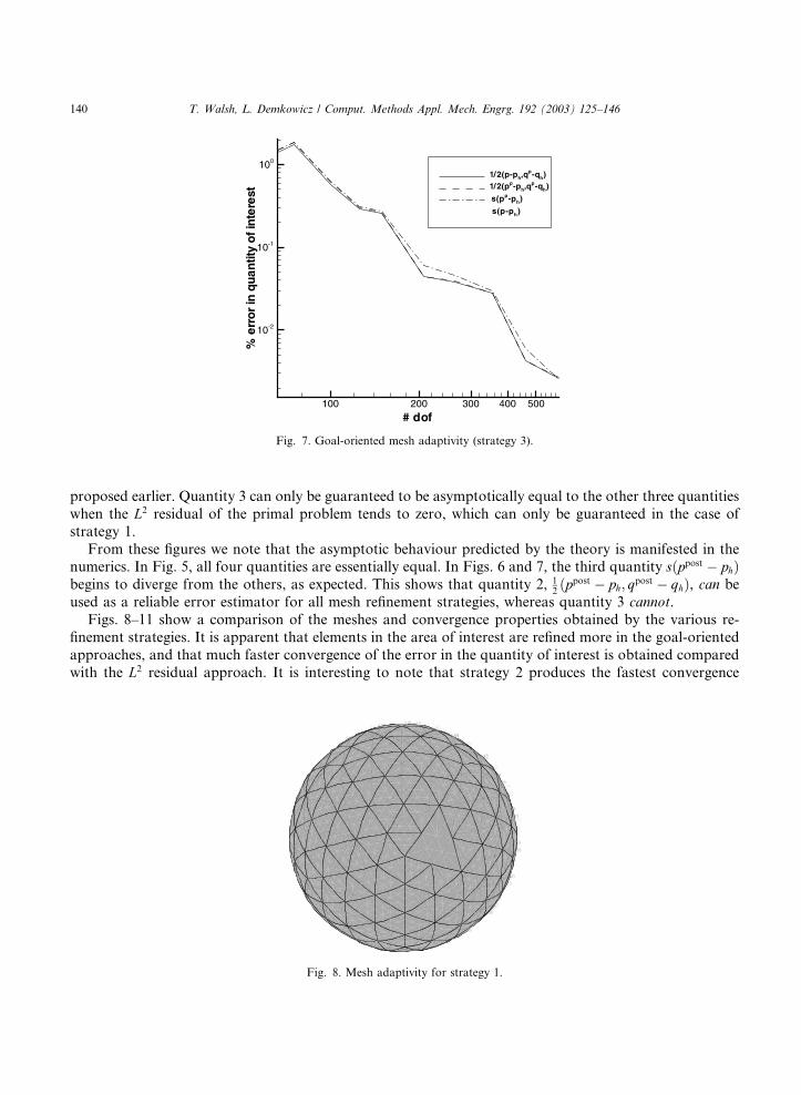
proposed earlier. Quantity 3 can only be guaranteed to be asymptotically equal to the other three quantities

when the L2 residual of the primal problem tends to zero, which can only be guaranteed in the case of

strategy 1.

From these figures we note that the asymptotic behaviour predicted by the theory is manifested in thenumerics. In Fig. 5, all four quantities are essentially equal. In Figs. 6 and 7, the third quantity sðppost � phÞbegins to diverge from the others, as expected. This shows that quantity 2, 1

2ðppost � ph; qpost � qhÞ, can be

used as a reliable error estimator for all mesh refinement strategies, whereas quantity 3 cannot.

Figs. 8–11 show a comparison of the meshes and convergence properties obtained by the various re-

finement strategies. It is apparent that elements in the area of interest are refined more in the goal-oriented

approaches, and that much faster convergence of the error in the quantity of interest is obtained compared

with the L2 residual approach. It is interesting to note that strategy 2 produces the fastest convergence

Fig. 7. Goal-oriented mesh adaptivity (strategy 3).

Fig. 8. Mesh adaptivity for strategy 1.


initially, but that after several levels of refinement. Strategy 3 results in a slightly faster overall convergence.

As expected, strategy 1 is the least effective in reducing the error in the quantity of interest.

4.1.2. The head problem

Fig. 12 shows the area of interest for the head mesh without ear canal, which consists of a small area

around the entrance to the ear canal. Fig. 13 compares typical meshes obtained for goal-oriented and L2

residual-based adaptivity for a plane wave scattering problem, and at first glance they look very similar.

However, a zoom on the area of interest reveals a different story, as shown in Fig. 14. Here significantelement clustering is seen in the goal-oriented case, whereas no refinements at all are seen in the L2 residual

case. Fig. 15 compares typical meshes for the two refinement strategies, in this case within the ear canal. In

this case the area of interest is the eardrum, which is at the end of the canal. Significantly more element

clustering is seen in the goal-oriented case.

Figs. 16 and 17 show estimates of the percent error in the quantity of interest for a scattering simulation

on the head without and with the canal, respectively, again using the estimate 12ðppost � ph; qpost � qhÞ. In




both cases strategy 3 outperforms. It should be noted, however, that in some cases of simulations on thehead, the meshes and error estimates obtained by strategies 1 and 3 were similar. This is in contrast to the

case of a sphere, where strategy 3 significantly outpeformed strategy 1 in all cases tested.

Fig. 11. Goal-oriented and L2 residual-based mesh adaptivity.

Fig. 12. The area of interest (indicated in red) for the scattering simulations on the head.


4.2. Multiple right-hand sides

Finally, we consider a comparison of strategies 1 and 3 in the case of multiple right-hand sides. In this

experiment the orientation of the incident plane wave was varied from 0� to 360�, at increments of 60�.

Fig. 13. Goal-oriented and L2 residual adaptivity applied to plane wave scattering from head/ear mesh.

Fig. 14. Goal-oriented and L2 residual adaptivity applied to plane wave scattering from head/ear mesh––a closeup of the area of

interest.

Fig. 15. Goal-oriented and L2 residual adaptivity applied to plane wave scattering from head/ear mesh––a closeup of the ear canal.


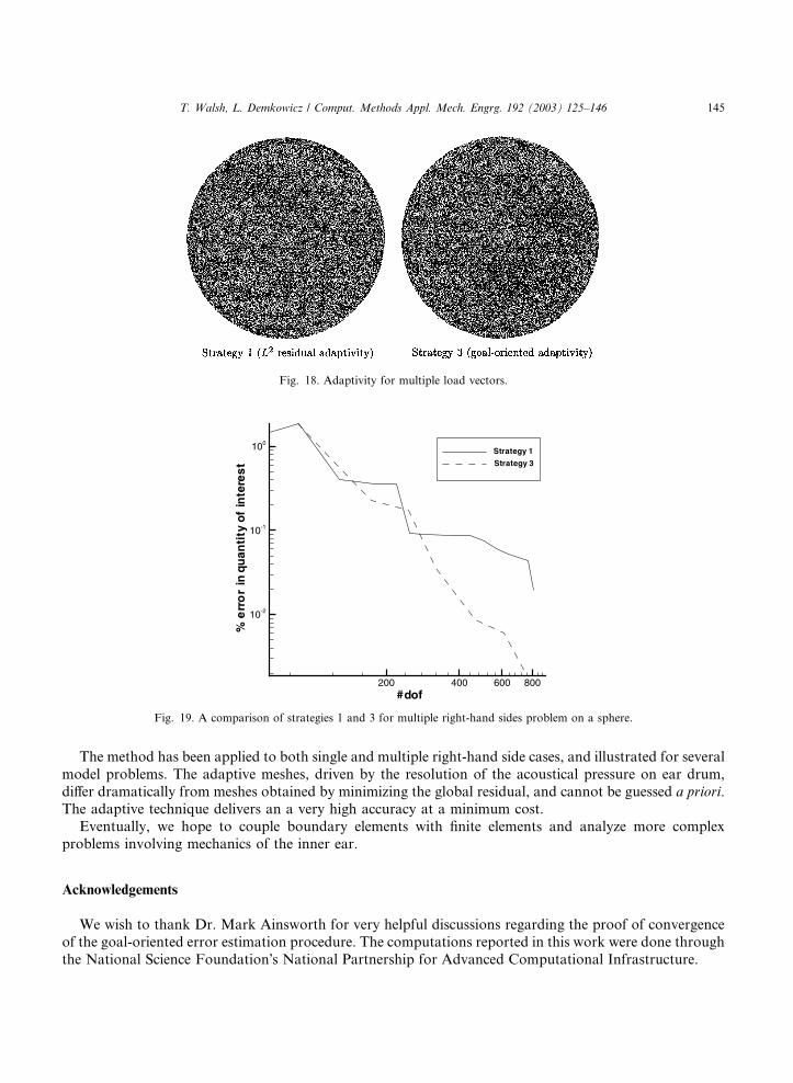
Using the procedure described above, a single mesh was generated that simultaneously resolved all six

solutions. Fig. 18 compares the meshes for the two cases, and they appear to have some resemblance to

Figs. 8 and 10, obtained for the single load case. Fig. 19 shows the maximum relative error in the quantity

of interest for all six solutions. We see that the goal-oriented procedure converged at a faster rate than the

L2 residual-based adaptivity procedure, for all right-hand sides.

5. Conclusions and future work

In the paper, a new goal-oriented error estimation technique, and a corresponding selective mesh re-

finement strategy for adaptive BEM, have been presented. The method generalizes the well known, ana-

logous technique used for adaptive FEMs [6,9,22–24], and builds upon the use of the L2 residual and

superconvergence for error estimation [8,11,12,17,18].

Fig. 16. Goal-oriented and L2 residual adaptivity applied to plane wave scattering from head/ear mesh, without ear canal.

Fig. 17. Goal-oriented and L2 residual adaptivity applied to plane wave scattering from head/ear mesh, with ear canal.


The method has been applied to both single and multiple right-hand side cases, and illustrated for several

model problems. The adaptive meshes, driven by the resolution of the acoustical pressure on ear drum,

differ dramatically from meshes obtained by minimizing the global residual, and cannot be guessed a priori.The adaptive technique delivers an a very high accuracy at a minimum cost.

Eventually, we hope to couple boundary elements with finite elements and analyze more complex

problems involving mechanics of the inner ear.

Acknowledgements

We wish to thank Dr. Mark Ainsworth for very helpful discussions regarding the proof of convergence

of the goal-oriented error estimation procedure. The computations reported in this work were done through

the National Science Foundation�s National Partnership for Advanced Computational Infrastructure.

Fig. 19. A comparison of strategies 1 and 3 for multiple right-hand sides problem on a sphere.

Fig. 18. Adaptivity for multiple load vectors.


References

[1] S. Amini, On the choice of the coupling parameter in boundary integral formulations of the exterior acoustic problem, Appl. Anal.

35 (1990) 75–92.

[2] I. Babu�sska, T. Strouboulis, K. Copps, S.K. Gangaraj, C. Upadhyay, a-posteriori error estimation for finite element and

generalized finite element method, TICAM Report 98-01, January 1998.

[3] C. Bajaj, G. Xu, Smooth reconstruction and deformation of free-form fat surfaces, TICAM report 99-08.

[4] C. Bajaj, Surface fitting with implicit algebraic surface patches, in: H. Hagen (Ed.), Topics in Surface Modeling, SIAM,

Philadelphia, PA, 1992, pp. 23–52.

[5] C. Bajaj, J. Chen, G. Xu, Modeling with cubic A-patches, ACM Trans. Graphics 14 (2) (1995) 103–133.

[6] R. Becker, R. Rannacher, Weighted a posteriori error control in FE method, ENUMATH-95, Paris, September 1995.

[7] A. Burton, G. Miller, The application of integral equation methods to the numerical solution of some exterior boundary-value

problems, Proc. Roy. Soc. London Ser. A 323 (1971) 201–210.

[8] Y. Chang, Scattering of acoustic waves on viscoelastic structures modeled by means of hp adaptive BE/FE methods, Doctoral

dissertation, The University of Texas at Austin, 1996.

[9] F. Cirak, E. Ramm, A posteriori error estimation and adaptivity for linear elasticity using the reciprocal theorem, Comput.

Methods Appl. Mech. Engrg. 156 (1998) 351–362.

[10] R. Ciskowski, Applications in bioacoustics, in: R. Ciskowski, C. Brebbia (Eds.), Boundary Element Method in Acoustics,

Computational Mechanics Publications, 1991.

[11] L. Demkowicz, J. Oden, M. Ainsworth, P. Geng, Solution of elastic scattering problems in linear acoustics using hp boundary

element methods, J. Comput. Appl. Math. 36 (1991) 29–63.

[12] L. Demkowicz, A. Karafiat, J.T. Oden, Solution of elastic scattering problems in linear acoustics using hp boundary element

method, Comput. Methods Appl. Mech. Engrg. 101 (1992) 251–282.

[13] L. Demkowicz, Asymptotic convergence in finite and boundary element methods: Part 2: The LBB constant for rigid and elastic

scattering problems, Comput. Math. Appl. 28 (6) (1994) 93–109.

[14] L. Demkowicz, K. Gerdes, C. Schwab, A. Bajer, T. Walsh, HP90: a general and flexible Fortran 90 hp-FE code, Comput.

Visualization Sci. 1 (1998) 145–163.

[15] L. Demkowicz, A. Bajer, K. Banas, Geometrical modeling package, TICOM Report 92-06, The University of Texas at Austin,

August 1992.

[16] N.A. Dumont, M.A.M. Noronha, A simple, accurate scheme for the numerical evaluation of quasi-singular, singular, and strongly

singular integrals, Comput. Mech. 22 (1998) 42–49.

[17] P. Geng, Parallel hp methods for coupled BE/FE analysis of structural acoustics problems, Doctoral dissertation, The University

of Texas at Austin, 1994.

[18] P. Geng, J.T. Oden, R.A. van de Geijn, Massively parallel computation for acoustical scattering problems using boundary element

methods, J. Sound Vibration 191 (1) (1996) 145–165.

[19] Y. Kahana, P. Nelson, M. Petyt, S. Choi, Numerical modeling of the transfer functions of a dummy-head and of the external ear,

in: AES 16th International Conference on Spatial Sound Reproduction, Finland, 1999.

[20] A. Karafiat, Analysis of boundary element method for acoustic scattering problems, Habilitation thesis, Politechnika Krakowska,

Krakow, 1996.

[21] B. Katz, Measurement and calculation of individual head related transfer functions using a boundary element model including the

measurement and effect of skin and hair impedance, Doctoral dissertation, The Pennsylvania State University, May 1998.

[22] M. Paraschivoiu, A.T. Patera, A hierarchical duality approach to bounds for the outputs of partial differential equations, Comput.

Methods Appl. Mech. Engrg. 158 (1998) 389–407.

[23] S. Prudhomme, J.T. Oden, On goal-oriented error estimation for elliptic problems: application to the control of pointwise errors,

Comput. Methods Appl. Mech. Engrg. 176 (1999) 313–331.

[24] S. Prudhomme, Adaptive control of error and stability of h–p approximations of the transient Navier–Stokes equations, Doctoral

dissertation, The University of Texas at Austin, 1999.

[25] E. Rank, Adaptive h, p, and hp versions for boundary integral element methods, IJNME 28 (1989) 1335–1349.

[26] E. Rank, Adaptivity and accuracy estimation for finite element and boundary integral element methods, in: I. Babuska, O.C.

Zienkiewicz, J. Gago, A.E. Oliveira, A. de (Eds.), Accuracy Estimates and Adaptive Refinements in Finite Element Computations,

Wiley, New York, 1986, pp. 79–84.

[27] C. Schwab, Variable order composite quadrature of singular and nearly singular integrals, Computing 53 (1994) 173–194.

[28] I.H. Sloan, Improvement by iteration for compact operator equations, Math. Comput. 30 (136) (1976) 758–764.

[29] R.A. van de Geijn, Using PLAPACK, The MIT Press, 1997.


hp boundary element modeling of the external human auditory system––goal-oriented adaptivity...

Documents