HPC et Mécanique des Fluides

A. Cadiou, Ch. PeraMarc Buat, Lionel Le Penven

Laboratoire de Mécanique des Fluides et d'AcoustiqueCNRS, Université Lyon I, École Centrale de Lyon, INSA de Lyon

École calcul intensif, Lyon, Septembre 2013

avec

Fluid Mechanics

Navier-Stokes equations

Claude Louis NAVIER

(1785-1836)

For incompressible ow, homogeneous uid

velocity U , pressure p

∂tU +U .∇U = −1/ρ ∇p + ν∆U

∇.U = 0

density ρ, viscosity ν

+ initial and boundary conditions

George Gabriel STOKES

(1819-1903)

Well-known equations, but open mathematical problems ....

Fluid Mechanics

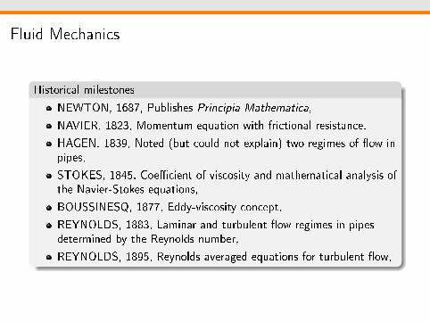
Historical milestones

NEWTON, 1687, Publishes Principia Mathematica,

NAVIER, 1823, Momentum equation with frictional resistance,

HAGEN, 1839, Noted (but could not explain) two regimes of ow inpipes,

STOKES, 1845, Coecient of viscosity and mathematical analysis ofthe Navier-Stokes equations,

BOUSSINESQ, 1877, Eddy-viscosity concept,

REYNOLDS, 1883, Laminar and turbulent ow regimes in pipesdetermined by the Reynolds number,

REYNOLDS, 1895, Reynolds-averaged equations for turbulent ow,

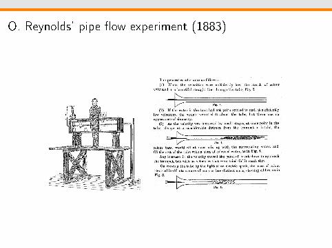
O. Reynolds' pipe ow experiment (1883)

Laminar/turbulent

Laminar jet Re = 2000

P. Chassaing, IMFT

Turbulent jet Re = 50000

P. Chassaing, IMFT

⇓

Observation :In the laminar jet, the uid layers are rectilinear.

When increasing the velocity, a transition is observed :layers oscillate, scramble and have a disorderly appearenceThe turbulent state is characterized by an agitated motion

Practical consequences of turbulence

Promote energy transfer to smaller scales and increase dissipation.

L

u

=⇒

Lη ≈ Re

3/4t

η Ret =uLν

Increase spatial transfer for mass, momentum, energy.

momentum transfer on solid wall ⇒ force,

y

T = µd<U>dy

T = µdUdy

Consequences may be favorable or not, depending on applications.

Example

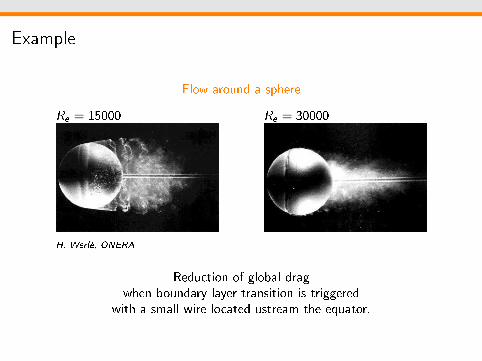
Flow around a sphere

Re = 15000

H. Werlé, ONERA

Re = 30000

H. Werlé, ONERA

Reduction of global dragwhen boundary layer transition is triggered

with a small wire located ustream the equator.

Example

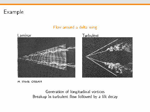
Flow around a delta wing

Laminar

H. Werlé, ONERA

Turbulent

H. Werlé, ONERA

Generation of longitudinal vorticesBreakup in turbulent ow followed by a lift decay

Near wall behaviour

Development of boundary layers

Laminar

M. Van Dyke

Turbulent

M. Van Dyke

Modication of turbulent properties in the wall vicinity

F. Laadhari, LMFA

Boundary layer : from analytical to numerical solution

Historical milestones

PRANDTL, 1904 Boundary-layer concept,

BLASIUS, 1908 Solution for laminar at-plate boundary layer,

VON KÁRMÁN 1921 Momentum integral theory for at-plate boundary layer,

PRANDTL, 1925, Mixing length concept,

TOLLMIEN, 1929, Theoretical critical Reynolds number for instability of thezero-pressure-gradient at-plate boundary layer,

NIKURADSE, 1933, Friction factor for articially-roughened pipes,

COLEBROOK and WHITE, 1937, transition formula for commercial pipe friction,

CLAUSER, 1954, Turbulent boundary layers with pressure gradient,

KLEBANOFF, 1955, Detailed experimental measurements in a at-plate boundary layer,

COLES, 1956, Law of the wake in the outer layer,

1968, Stanford Conference: Computing the turbulent boundary layer,

SPALART, 1988, Direct numerical simulation of a turbulent at-plate boundary layer upto Re = 1400.

D. Apsley, University of Manchester

L.F. Richardson's numerical solution (1910)

Lewis Fry RICHARDSON

(1881-1953)

Weather forecast calculation (V. Bjerknes, 1904)

First numerical solutionto dierential equation, by hand, 1910⇒ predict at a single point locationa pressure change in weather over a six-hour period⇒ took him six weeks to calculateand the prediction turned out to becompletely unrealistic

"Weather Forecast Factory",with 64000 people (human computer)

Computational Fluid Dynamics

Milestones

RICHARDSON, 1910, hand calculation, 2000 operations per week

Relaxation methods (1920's-50's), solve potential linearizedequations

COURANT, FRIEDRICHS and LEWY, 1928, Landmark paper forhyperbolic equations

VON NEUMANN, 1950, Stability criteria for parabolic problems

RICHARDSON, 1950, Climate prediction on ENIAC, iterativemethod

HARLOW and FROMM, 1963, computed unsteady vortex streetusing a digital computer

PATANKAR and SPALDING, 1972, Solution techniques forincompressible ows (SIMPLE)

JAMESON, 1981, Compute Euler ow over complete aircraft

Computational challenge

Mainly associated to the resolution of small-scale turbulence phenomena

Wide range of spatial and temporal scales

Large scale L, scale of most kinetic energy containing eddies

Kolmogorov scale η, smallest eddies

L

η= Re

3/4t

where Ret = uL/ν turbulent Reynolds number,u turbulent velocity scale

η =

(ν3

ε

)1/4 where ε dissipation of turbulent kinetic energyK = 2/3 u2

Taylor scale λ, most dissipative eddies ε = 15 ν u2

λ2

Scale speparation increases with Rλ ∼ Re1/2t

Atmospheric ows Re ∼ 108

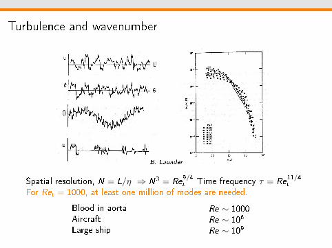
Turbulence and wavenumber

B. Launder

Spatial resolution, N = L/η ⇒ N3 = Re9/4t Time frequency τ = Re

11/4t

For Ret = 1000, at least one million of modes are needed.

Blood in aortaAircraftLarge ship

Re ∼ 1000Re ∼ 106

Re ∼ 109

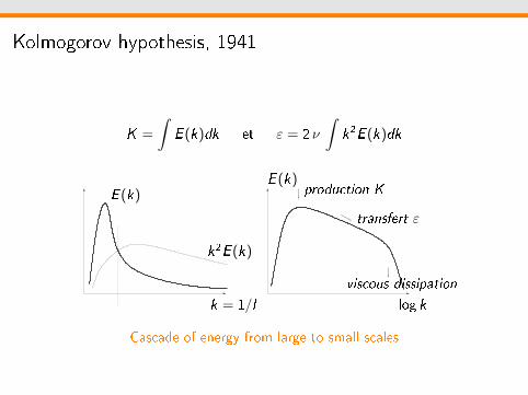
Kolmogorov hypothesis, 1941

K =

∫E (k)dk et ε = 2 ν

∫k2E (k)dk

E (k)

k2E (k)

k = 1/l

E (k)production K

viscous dissipation

log k

transfert ε

Cascade of energy from large to small scales

Numerical simulation of turbulence

Historical milestones

Orszag 1969-1971: spectral and pseudo-spectral methods

Riley and Patterson, 1972: particle tracking (323), Rλ ∼ 35

Leonard, 1974: large-eddy simulation

Rogallo, 1981: homogeneous turbulence (1283)

Kim, Moin and Moser, 1987: channel ow (Chebyshev)

5123 simulations, Rλ ∼ 200

Kaneda, Ishihara, Yokokawa, Itakura and Uno, 2002: 40963 on EarthSimulator, Japan, Rλ ∼ 1200

Wide range of numerical methods and strategies for CFD

Eulerian methods

Finite Dierence Method (FDM),

Finite Element Method (FEM),

Finite Volume Method (FVM),

Spectral Methods

Particle methods

lattice gas automata (LGA),

lattice Boltzmann equation (LBE),

discrete velocity methods (DVM),

dissipative particle dynamics (DPD),

smoothed-particle hydrodynamics (SPH),

direct simulation Monte Carlo (DSMC),

stochastic rotation dynamics (SRD),

molecular dynamics (MD)

Hybrid methods

Coupled Eulerian/Lagrangian methods

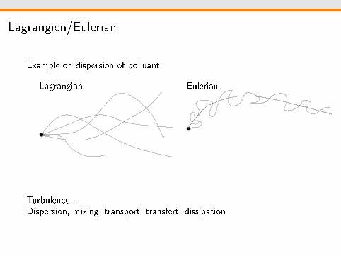
Lagrangien/Eulerian

Example on dispersion of polluant

Lagrangian Eulerian

Turbulence :Dispersion, mixing, transport, transfert, dissipation

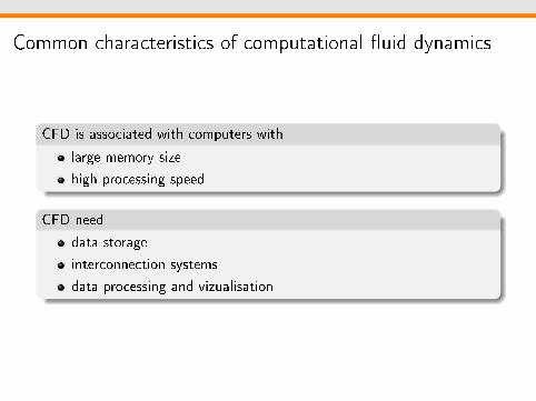
Common characteristics of computational uid dynamics

CFD is associated with computers with

large memory size

high processing speed

CFD need

data storage

interconnection systems

data processing and vizualisation

CFD process

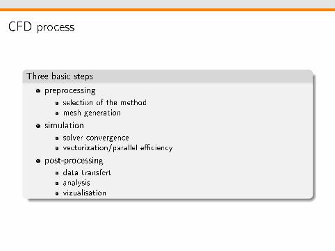
Three basic steps

preprocessingselection of the methodmesh generation

simulationsolver convergencevectorization/parallel eciency

post-processingdata transfertanalysisvizualisation

Fluid Mechanics and GENCI resources

Increasing number of project requesting more than 1 million of core hours.Largest projects in

CT2 (mécanique des uides, uides réactifs, uides complexes),

CT4 (astrophysique et géophysique),

CT5 (physique théorique et physique des plasmas),

...

What is expected from HPC resources ?

V. Moureau, CORIA

Complex geometry and coupled physics.FV solver for massively parallel platforms. 2.6 billions of tetrahedrons.

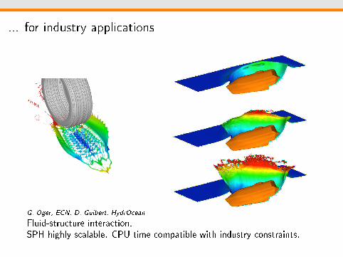
... for industry applications

G. Oger, ECN, D. Guibert, HydrOcean

Fluid-structure interaction.SPH highly scalable. CPU time compatible with industry constraints.

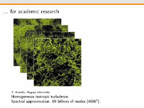
... for academic research

Y. Kaneda, Nagoya University

Homogeneous isotropic turbulence.Spectral approximation. 69 billions of modes (40963).

What did we learn ?

Y. Kaneda et al., 2003

Catch the tail of universality by scalingDiculty : small scale activity dominated by dissipation and enstrophyIntermittency : strong localized uctuations in space and time at high Rλ

What is expected from larger resolution ?

D. Donzis

Le Laboratoire de Mécanique des Fluides et d'Acoustique

Domaines de recherche

Physique et modélisation de la turbulence,

instabilités hydrodynamiques,

écoulements diphasiques,

mécanique des uides environnementale,

aérodynamique interne,

phénomènes thermiques couplés,

aéroacoustique,

propagation acoustique,

méthodes de résolution numérique des équations de Navier-Stokes,

contrôle actif ou passif des écoulements,

microuidique.

Le Laboratoire de Mécanique des Fluides et d'Acoustique

Secteurs d'application et partenaires industriels

Aéronautique et Spatial : SAFRAN/SNECMA, CNES, ONERA,Turbomeca, EADS, Dassault

Automobile Renault, Volvo, Valeo, Delphi, IAV, CNRT, PO, PôlesLUTB, Moveo, ID4car

Environnement - Bruit DGA, CNES, ONERA, SNCF, Eurocopter,EADS, PSA, CEA DAM

Environnement - atmosphérique, hydrologique EDF, INERIS,CEA, CEMAGREF, Total, Londres, Turin, Air Parif...

Génie des procédés, Energie CEA, Aventis, Geoservices, Andritz...

Computational challenge:Numerical experiments of turbulent transitionof spatially evolving ows

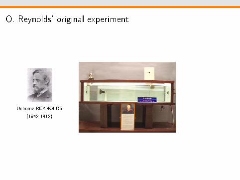
O. Reynolds' original experiment

Osborne REYNOLDS

(1842-1912)

Dye visualization

N.H Johannesen, C. Lowe

Critical Reynolds number

Re pipe Poiseuilleexp. ∼ 2000 ∼ 1000crit. ∞ 5772

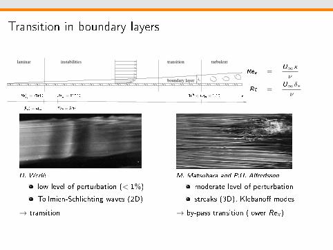
Transition in boundary layers

boundary layer

transitioninstabilitieslaminar turbulent

Rec = 520

Rexc = 91080

Re ′c = 461

Re ′xc = 71680 105 < Rext < 3.106 x

δ∗

Rex =U∞x

ν

Re =U∞δ∗

ν

H. Werlé

low level of perturbation (< 1%)

Tollmien-Schlichting waves (2D)

→ transition

M. Matsubara and P.H. Alfredsson

moderate level of perturbation

streaks (3D), Klebano modes

→ by-pass transition (lower Rex )

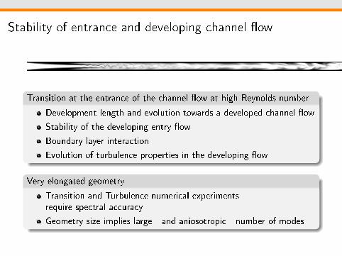
Stability of entrance and developing channel ow

Transition at the entrance of the channel ow at high Reynolds number

Development length and evolution towards a developed channel ow

Stability of the developing entry ow

Boundary layer interaction

Evolution of turbulence properties in the developing ow

Very elongated geometry

Transition and Turbulence numerical experimentsrequire spectral accuracy

Geometry size implies large - and aniosotropic - number of modes

Spectral approximation

Numerical experiment: need to resolve the ow at all scales .

As(Lη

)3∼ Re9/4 , increasingly stringent condition for turbulence.

Spectral methods are attractive, due to their high spatial accuracy.

Spatial derivatives are calculatedexactly.

Exponential convergence forsmooth solutions (faster than FE,FD ...).

0 1 2 3kh

1

0

(dudx)h−dudx

spectral

DF order 2

DF order 4

Since the 70's, extensively applied to simulation of turbulent owsbut, their implementation on new HPC must be carefully considered.

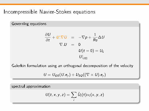
Incompressible Navier-Stokes equations

Governing equations

∂U

∂t+ U.∇U = −∇p +

1Re

∆U

∇.U = 0

U(t = 0) = U0

U|∂Ω

Galerkin formulation using an orthogonal decomposition of the velocity

U = UOS(U.ey ) + USQ((∇× U).ey )

spectral approximation

U(t, x , y , z) =∑i

Ui (t)αi (x , y , z)

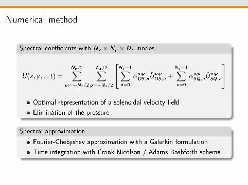
Numerical method

Spectral coecients with Nx × Ny × Nz modes

U(x , y , z , t) =

Nx/2∑m=−Nx/2

Nz/2∑p=−Nz/2

Ny−1∑n=0

αmpOS,nUmpOS,n +

Ny−1∑n=0

αmpSQ,nUmpSQ,n

Optimal representation of a solenoidal velocity eld

Elimination of the pressure

Spectral approximation

Fourier-Chebyshev approximation with a Galerkin formulation

Time integration with Crank Nicolson / Adams Bashforth scheme

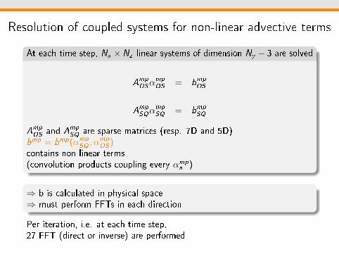
Resolution of coupled systems for non-linear advective terms

At each time step, Nx ×Nz linear systems of dimension Ny − 3 are solved

AmpOSα

mpOS = b

mpOS

AmpSQα

mpSQ = b

mpSQ

AmpOS and A

mpSQ are sparse matrices (resp. 7D and 5D)

bmp = bmp(αmpSQ , αmpOS)

contains non-linear terms(convolution products coupling every αmpn )

⇒ b is calculated in physical space⇒ must perform FFTs in each direction

Per iteration, i.e. at each time step,27 FFT (direct or inverse) are performed

Challenge: from 100 to 10000 cores OutlineExample of conguration: computational domain size 280× 2× 6.4

34560× 192× 768 modes (∼ 5. billions of modes)

travel 1 length with it=600000 iterations. (∼ 16 millions of FFT)

Memory constraint

N = Nx × Ny × Nz , with N very large

- large memory requirement (∼ 2To)

- BlueGene/P 0.5 Go per core ⇒ ∼ 4000 cores needed

Nx >> Ny ,Nz , elongated in one direction

- 1D domain decomposition ⇒ limited to ∼ 100 cores

- can only simulate a 40 times shorter channel length

Wall clock time constraint

CPU time 150h ∼ 6 days on ∼ 16000 cores

- with 100 cores (if possible), 160 times slower, 24000h ∼ 3 years

Implementation on HPC platforms

MPI strategy to scale from O(100) to O(10 000) core

Hybrid strategy to migrate on many-core platform

Additional constraint for optimization

Data manipulation during simulation

Data manipulation for analysis and post-treatment

2D domain decomposition Outline

SPECTRAL SPACE

SPECTRAL SPACE

PHYSICAL SPACEudu/dx

Non linear terms

udu/dx

Non linear terms

udu/dx

FFT inverse axe x

FFT axe x

FFT inverse axe z

FFT axe z

Chebyshev between walls(y direction, Ny + 1 modes)

2D FFT in periodical directions(x direction and z direction)

Transpose fromy−pencil to x−pencil,x−pencil to z−pencil and back

Increase the number of MPI processes and reduce wall clock time

1D decomposition: MPI ≤ Ny

34560× 192× 768 → max. of MPI processes: nproc=192

2D decomposition: MPI ≤ Ny × Nz

34560× 192× 768 → max. of MPI processes: nproc=147 456

Perform data communications and remapping

Choose data rearrangement to limit the increase in communications

Implementation on HPC platforms

MPI strategy to scale from O(100) to O(10 000) core

Hybrid strategy to migrate on many-core platform

Additional constraint for optimization

Data manipulation during simulation

Data manipulation for analysis and post-treatment

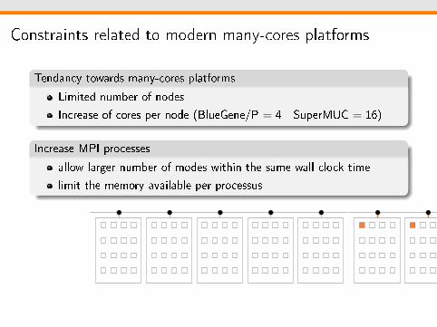
Constraints related to modern many-cores platforms

Tendancy towards many-cores platforms

Limited number of nodes

Increase of cores per node (BlueGene/P = 4 - SuperMUC = 16)

Increase MPI processes

allow larger number of modes within the same wall clock time

limit the memory available per processus

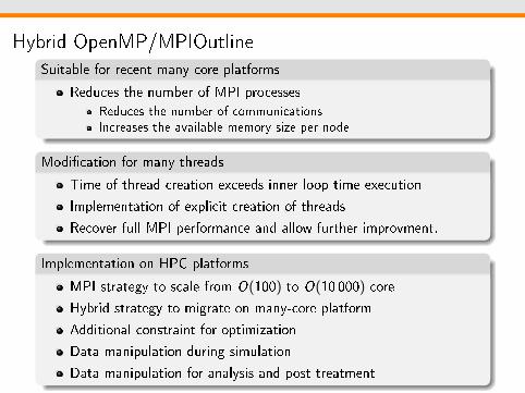
Hybrid OpenMP/MPIOutlineSuitable for recent many-core platforms

Reduces the number of MPI processesReduces the number of communicationsIncreases the available memory size per node

Modication for many threads

Time of thread creation exceeds inner loop time execution

Implementation of explicit creation of threads

Recover full MPI performance and allow further improvment.

Implementation on HPC platforms

MPI strategy to scale from O(100) to O(10 000) core

Hybrid strategy to migrate on many-core platform

Additional constraint for optimization

Data manipulation during simulation

Data manipulation for analysis and post-treatment

More than domain decomposition ...OutlineTasks parallelization : mask communications by execution time

reduces by 20% time per iteration

less loss in communications - waist ∼ 10%

Placement of processus

specic on each platform, optimize interconnection communications

avoid threads to migrate from one core to another

example: TORUS versus MESH in BlueGene/P platform - 50% faster

Implementation on HPC platforms

MPI strategy to scale from O(100) to O(10 000) core

Hybrid strategy to migrate on many-core platform

Additional constraint for optimization

Data manipulation during simulation

Data manipulation for analysis and post-treatment

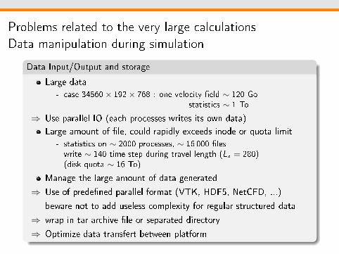
Problems related to the very large calculationsData manipulation during simulation

Data Input/Output and storage

Large data- case 34560× 192× 768 : one velocity eld ∼ 120 Go

statistics ∼ 1 To

⇒ Use parallel IO (each processes writes its own data)

Large amount of le, could rapidly exceeds inode or quota limit- statistics on ∼ 2000 processes, ∼ 16 000 les- write ∼ 140 time step during travel length (Lx = 280)(disk quota ∼ 16 To)

Manage the large amount of data generated

⇒ Use of predened parallel format (VTK, HDF5, NetCFD, ...)

beware not to add useless complexity for regular structured data

⇒ wrap in tar archive le or separated directory

⇒ Optimize data transfert between platform

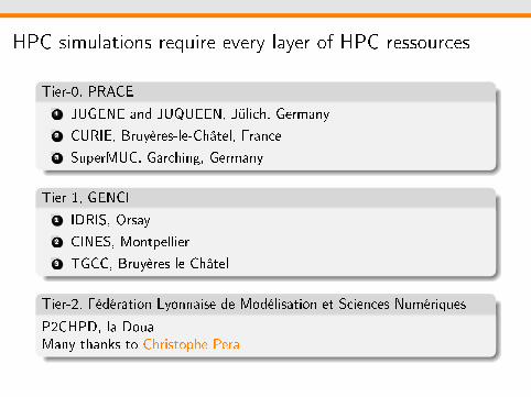
HPC simulations require every layer of HPC ressources

Tier-0, PRACE1 JUGENE and JUQUEEN, Jülich, Germany2 CURIE, Bruyères-le-Châtel, France3 SuperMUC, Garching, Germany

Tier-1, GENCI1 IDRIS, Orsay2 CINES, Montpellier3 TGCC, Bruyères-le-Châtel

Tier-2, Fédération Lyonnaise de Modélisation et Sciences Numériques

P2CHPD, la DouaMany thanks to Christophe Pera

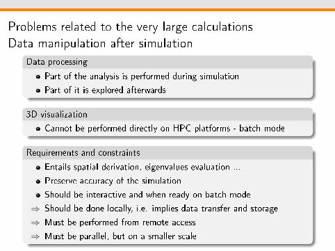
Problems related to the very large calculationsData manipulation after simulation

Data processing

Part of the analysis is performed during simulation

Part of it is explored afterwards

3D visualization

Cannot be performed directly on HPC platforms - batch mode

Requirements and constraints

Entails spatial derivation, eigenvalues evaluation ...

Preserve accuracy of the simulation

Should be interactive and when ready on batch mode

⇒ Should be done locally, i.e. implies data transfer and storage

⇒ Must be performed from remote access

⇒ Must be parallel, but on a smaller scale

Example

Simulation (multi-run batch) onLRZ SUPERMUC∼ 5 billions of modes34560× 192× 768run with ∼ 1s/dt on 16 384 cores2048 partitions

Analysis of the Big Data

In situ analysis not possible(batch and remote display)=⇒transfert of data=⇒parallel analysis mandatory=⇒script mode mandatory(reproductible)

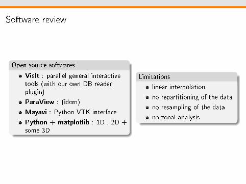
Software review

Open-source softwares

VisIt : parallel general interactivetools (with our own DB readerplugin)

ParaView : (idem)

Mayavi : Python VTK interface

Python + matplotlib : 1D , 2D +some 3D

Limitations

linear interpolation

no repartitioning of the data

no resampling of the data

no zonal analysis

Parallel client-server analysis tools

Parallel server

automatic repartitioning

resampling of the data

spectral interpolation

Python + NUMPY +MPI4PY + SWIG

Python UDF

Multiple clients1 matplotlib 1D + 2D2 mayavi lib 3D visualization3 VisIt 3D //e visualization

(using libsim, i.e. wo le)

Python + UDF + script

TCP connection

Workow for the analysis

Client screen

In situ (real computational time) analysis

Requirements

Analysis at a lower parallel scalethan the simulation

Pertinent variables for analysis farfrom simulations variables

Should know what andwhere to look at

Being able to repeat simulations⇒ fast enough

Act on simulation parameters(like in experiment)

Open-source software

VisIt

ParaView

Python + matplotlib

Limitations

should be run with the samegranularity as the simulation

no zonal analysis

no resampling of the data

poor accuracyin spatial operators

speed of calculation

Parallel in situ analysis tool

HP

Coupling of HPC simulation and visualization

Analysis of large 4D data Solve the I/O bottleneck Interactive visualization of time

dependant problem

projet hébergé EQUIP@MESO

In-situ visualizationof very large CFD simulations

Simulation code (O 1000 cores)

Analysis code (O 100 cores)

In situ co-processing Interpolation, data processing

PluginLibsim

Visit

PluginPython Numpy

Matplotlib

HPC Cluster

Visualizationworkstation

MPI

socket

socketScript python

Equipe aero-interne

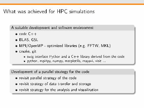
What was achieved for HPC simulations

A suitable development and software environment

code C++

BLAS, GSL

MPI/OpenMP - optimized libraries (e.g. FFTW, MKL)

cmake, gitswig interface Python and a C++ library derived from the codepython, mpi4py, numpy, matplotlib, mayavi, visit ...

Development of a parallel strategy for the code

revisit parallel strategy of the code

revisit strategy of data transfer and storage

revisit strategy for the analysis and visualization

Resulting method

Characterictics

Ecient solver for hybrid multicore massively parallel platformsOriginal coarse grained MPI/OpenMP strategyTasks overlapping

Pre- and post- processing tools for smaller MPI platformsparallel VTK format (paraview)Parallel Client/Server programs in Python calling a spectral library2D/3D parallel visualization - (matplotlib/mayavi/visit)

Properties

Fairly portable

Small time spent in communications ∼ 10%

Rapid wall clock time for a global scheme(1 billion of modes: 1.3s/it on BlueGene/P - 0.2s/it on SuperMUC)

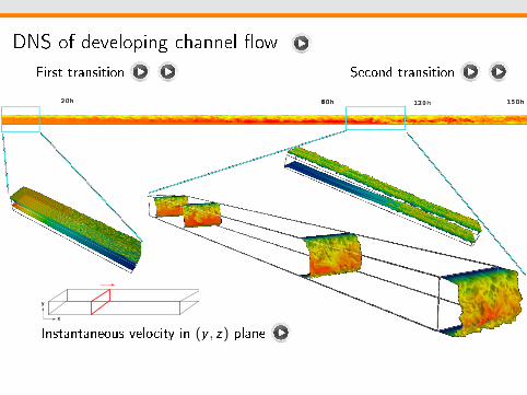
DNS of developing channel ow

First transition Second transition

x

y

Instantaneous velocity in (y , z) plane

DNS of turbulent transition in channel entrance ow

Parametric study with the Reynolds number

At high Reynolds number, similarity with the Boundary Layer instabilityAt low Reynolds number, the optimal mode has 180 phase shiftbetween up and low array of vortices

Identication of two non-linear streaks instability

Large amplitude of the optimalperturbation

Varicose instability

Small amplitude of the optimalperturbation

Sinuous instability

decaying amplitude of pertubation

Fédération Lyonnaise de Modélisation et SciencesNumériques

La FLMSN regroupe l'ancienne structure fédérative Fédération Lyonnaise

de Calcul Haute Performances (FLCHP), L'Institut rhône-alpin des

systèmes complexes (IXXI) et le Centre Blaise Pascal (CBP)

La FLMSN est une structure fédérative qui regroupe un méso-centre decalcul HPC pour la région lyonnaise, et deux structures d'animations etde recherche autour de la modélisation numérique et du calcul HPC :l'IXXI et le CBP.Le méso-centre FLCHP a des infrastructures localisées sur 3 sites

le site de la DOUA (P2CHPD avec PRABI)pour l'Université Lyon1, l'INSA de Lyon

le site de Gerland (PSMN) pour l'ENS Lyon

le site d'Écully (PMS2I) pour l'ECL Lyon

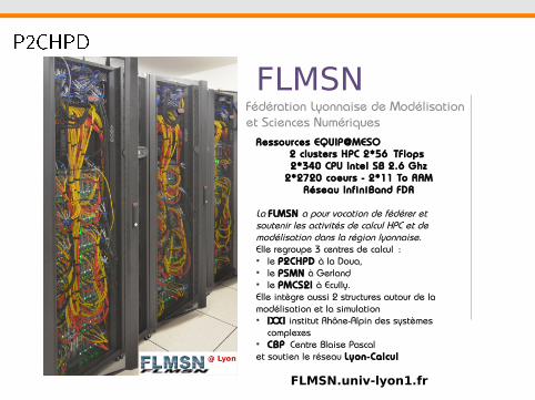
P2CHPD

Ressources EQUIP@MESO2 clusters HPC 2*56 TFlops 2*340 CPU Intel SB 2.6 Ghz

2*2720 coeurs - 2*11 To RAMRéseau InfiniBand FDR

La FLMSN a pour vocation de fédérer et soutenir les activités de calcul HPC et de modélisation dans la région lyonnaise. Elle regroupe 3 centres de calcul : le P2CHPD à la Doua, le PSMN à Gerland le PMCS2I à Ecully.Elle intègre aussi 2 structures autour de la modélisation et la simulation IXXI institut Rhône-Alpin des systèmes

complexes CBP Centre Blaise Pascal et soutien le réseau Lyon-Calcul

FLMSN.univ-lyon1.fr

Fédération Lyonnaise de Modélisation et Sciences Numériques

FLMSN

2D Parallel strategy - illustration

64 128 256 512 1024 2048 4096number of cores

10-1

100

101

time

1D2D

Figure : Time per iteration for a 1024× 256× 256 case.

improve the maximum of MPI processes

could be limited by memory availability

OpenMP

64 128 256 512 1024 2048 4096number of cores

10-1

100

101

time

T1T8

64 128 256 512 1024 2048 4096number of cores

10-1

100

101

time

T1T2T4T8

Figure : Time per iteration for a 1024× 256× 256 case.

Suitable for recent many-core platforms

Reduces the number of MPI processesReduces the number of communicationsIncreases the available memory size per node

Implementation of explicit creation of threadsCoarse grained OpenMP needed for fast inner loopDene a new synchronization barrier

Speedup and eciency

2048 4096 8192 16384ncore

10242048

4096

8192

16384

spee

dup

idealBabel

2048 4096 8192 16384ncore

0.0

0.2

0.4

0.6

0.8

1.0

1.2

1.4

effic

ienc

y

idealBabel

Figure : 4096× 512× 512 ∼ 109 modes

Decent wall clock time :109 modes : 0.9 s/iteration for 16384 cores

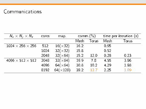
Communications

Nx × Ny × Nz cores map. comm.(%) time per iteration (s)Mesh Torus Mesh Torus

1024× 256× 256 512 16(×32) 16.2 - 0.95 -1024 32(×32) 15.8 - 0.52 -2048 32(×64) 15.2 12.0 0.28 0.23

4096× 512× 512 2048 32(×64) 19.9 7.8 4.55 3.964096 64(×64) 30.8 10.2 4.29 1.988192 64(×128) 39.2 12.7 2.25 1.09

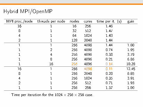
Hybrid MPI/OpenMP

MPI proc./node threads per node nodes cores time per it. (s) gain16 1 16 256 1.468 1 32 512 1.474 1 64 1024 1.432 1 128 2048 1.441 1 256 4096 1.44 1.001 2 256 4096 0.74 1.951 4 256 4096 0.38 3.791 8 256 4096 0.21 6.861 16 256 4096 0.14 10.2816 1 256 4096 0.11 12.458 1 256 2048 0.20 6.854 1 256 1024 0.35 3.912 1 256 512 0.71 1.931 1 256 256 1.37 1.00

Time per iteration for the 1024× 256× 256 case.

To read more :J. Montagnier, A. Cadiou, M. Buat, L. Le Penven,Towards petascale spectral simulations for transition analysis in wall

bounded ow (2012), Int. Journal for Numerical Methods in Fluids,doi:10.1002/d.3758