HPC I/O Throughput Bottleneck Analysis withExplainable Local Models

Mihailo Isakov∗, Eliakin del Rosario∗, Sandeep Madireddy†,Prasanna Balaprakash†, Philip Carns†, Robert B. Ross†, Michel A. Kinsy∗

∗ Adaptive and Secure Computing Systems (ASCS) LaboratoryDepartment of Electrical and Computer Engineering, Texas A&M University, College Station, TX 77843

{mihailo,eliakin.drosario,mkinsy}@tamu.edu† Argonne National Laboratory, Lemont, IL 60439

smadireddy@anl.gov, {pbalapra,carns,rross}@mcs.anl.gov

Abstract—With the growing complexity of high-performancecomputing (HPC) systems, achieving high performance can bedifficult because of I/O bottlenecks. We analyze multiple years’worth of Darshan logs from the Argonne Leadership ComputingFacility’s Theta supercomputer in order to understand causes ofpoor I/O throughput. We present Gauge: a data-driven diagnostictool for exploring the latent space of supercomputing job features,understanding behaviors of clusters of jobs, and interpretingI/O bottlenecks. We find groups of jobs that at first sight arehighly heterogeneous but share certain behaviors, and analyzethese groups instead of individual jobs, allowing us to reducethe workload of domain experts and automate I/O performanceanalysis. We conduct a case study where a system owner usingGauge was able to arrive at several clusters that do not conformto conventional I/O behaviors, as well as find several potentialimprovements, both on the application level and the system level.

Index Terms—HPC, I/O, diagnostics, machine learning, clus-tering

I. INTRODUCTION

Because of the scale and evolving complexity of high-performance computing (HPC) systems, critical gaps stillremain in our understanding of HPC applications’ runtimebehaviors, specifically, compute, communication, and storagebehaviors. This situation is further complicated by the factthat HPC applications come from a diverse set of scientificdomains, can have vastly different characteristics, and are exe-cuted simultaneously, thereby contending for shared resources.

One such gap is the understanding of I/O utilization inthese systems. Currently, application programmers and sys-tems administrators still heavily rely on limited observations,anecdotes, and scattered experiences to develop design patternsfor applications and manage their runtime performance eitherat the node level or at the system level. This approach istractable only to the extent permitted by limited applicationdeveloper and facility support staff resources and their exper-tise. Therefore, automated data-driven methods are needed tostreamline this process and reduce the turnaround time fromcapturing information to understanding and enacting improve-ments in I/O utilization and efficiency. One intuitive way toapproach this situation is not by simply considering applicationperformance in isolation but by identifying commonalitiesthat reduce the volume of characterization data, simplify

KiB MiB GiB TiB PiB

I/O Volume

KiB / s

MiB / s

GiB / s

TiB / s

I/O

Th

rou

ghp

ut

1 16 256 4096 65536Number of processes

100

101

102

103

104

Nu

mb

erof

job

s

Fig. 1: Frequency of jobs with respect to I/O throughput andthe total number of bytes transferred. Data are collected fromthe Argonne Leadership Computing Facility (ALCF) Thetasupercomputer. Note that the color bar is logarithmic.

performance modeling efforts, and exploit opportunities forperformance improvement across application domains.

Machine learning (ML) is a promising approach for thedata-driven analysis of I/O performance data. This is evidencedby the growing interest in the design and development ofML-based methods for various I/O performance analysis andmodeling tasks [1]–[6]. However, analyzing I/O performanceis not trivial. Figure 1 shows that I/O throughput spansalmost 14 orders of magnitude and can vary as much as fiveorders of magnitude for jobs with the same amount of I/Ovolume. Given the complexity of the I/O performance data,the relationship between the I/O performance and the factorsthat affect it are often nonlinear. Consequently, there is atrade-off between explainability and predictive accuracy whenout-of-the-box ML methods are adopted for I/O performanceanalysis. In particular, the models that are explainable andintuitive to I/O experts are often simple and based on linearmodels. The models that have high predictive accuracy areoften black box and cannot be used directly for explaining theI/O performance.

We develop an explainable ML platform for I/O perfor-mance analysis to answer a number of I/O performancequestions: how can we cluster applications together? Givenan application or task execution, what existing I/O behaviorcluster does the job fall into? What are the key characteristicsof the cluster itself? Does it match the expected executionor performance profile, for example, the requested resources

SC20, November 9-19, 2020, Is Everywhere We Are978-1-7281-9998-6/20/$31.00 ©2020 IEEE

and the optimality of those resources’ utilization? How doesthis job’s performance rank with the rest of the cluster? Whatparameters influence the job placement within the cluster?How does the cluster rank with other clusters?The goal of this work is to answer these questions, and to thisend our contributions are as follows:

• We introduce a log-based feature engineering pipeline forHPC applications. Our analysis uses 89,844 Darshan logs ofI/O volume greater than 100 MiB collected on the ArgonneLeadership Computing Facility (ALCF) Theta supercom-puter from 2017 to 2020.

• We show that agglomerative clustering can reveal a largeamount of structure in the dataset and that training modelson fine-grained (local) clusters instead of on the wholedataset yields more robust and useful predictions.

• Using different ML methods, we demonstrate that despiteI/O throughput varying across many orders of magnitude,we can on average predict individual job I/O throughputwithin ∼20% of the real value. Furthermore, we show howthe interpretation of ML prediction models can yield usefuladvice for increasing application performance.

• To validate the practicality of the proposed feature engi-neering pipeline and the clustering techniques, we introduceGauge, an exploratory I/O throughput analysis tool withadjustable data granularity and interpretable I/O throughputmodels. We illustrate how it can be used by system ownersand I/O experts to optimize the HPC clusters for theworkload present or by application developers to optimizetheir jobs.

• We release a web-based version of Gauge, information aboutthe tool is available at http://ascslab.org/research/gauge.

II. EXPLORATION OF THE APPLICATION SPACE

A. Darshan Log Dataset GenerationDarshan [6] is an HPC I/O characterization tool that

transparently captures I/O access pattern information aboutapplications running on a system. It collects information suchas numbers of POSIX operations, I/O access patterns withinfiles, and timestamps of events such as opening or closing files.We have collected 661,553 Darshan logs from the ALCF’sTheta supercomputer, ranging from January 2017 to March2020. Since using Darshan is optional and as many legacyapplications do not support it, our dataset covers only 28% ofall jobs run on Theta.

For each job, Darshan can be used with a number of instru-mentation modules, such as POSIX, MPI-IO, stdio, HDF5, andLustre. In this work, since we focus on I/O characterization,two modules are of interest: POSIX and MPI-IO. We chooseto use only POSIX for two reasons: (1) since the MPI-IO layerpasses through the POSIX layer, POSIX operation counters arestrictly equal to or larger than that of MPI-IO and (2) MPI-IO requires POSIX to be enabled, but only 28.2% of the jobsinstrumented with POSIX are also instrumented with MPI-IO.

The POSIX module measures 86 features, such as numberof bytes read and written; number of accesses per each of

the 10 bins; number of consecutive and sequential read andwrite operations; file and memory aligned operations; sizesand strides of the top four most common POSIX accesssizes; number of common POSIX calls such as seek(),stat(), and fsync(); cumulative time spent reading,writing, and in other operations such as seek(), stat(),and fsync(); and timestamps of the first and last POSIXopen/read/write/close operations. More information can befound in the Darshan-util documentation [7]. On top of thisset, we appended 10 Darshan metaparameters including thejob’s I/O throughput; number of unique or shared files opened;and number of read-only, read/write, and write-only files. Logscontaining all of these features serve as the raw dataset, whichwe process with a data sanitization and normalization pipelinedescribed below.

B. Sanitization and Normalization PipelineOur data preprocessing pipeline consists of several steps:

1) Data sanitization: In this step, we remove jobs that arenot instrumented with POSIX or have invalid values (e.g.,negative values). Negative values are typically presentwhen a job was not closed properly or when a hardwarefault occurred. Similarly, we remove features that have alarge number of missing values. These typically arise sincethe version of Darshan running on Theta has changed overthe years and new features were introduced. Hence, wechoose to ignore these new features.

2) Feature pruning: We remove common access size featuresand all time-sensitive features. Common access size fea-tures store the most common access sizes in bytes. Becauseof the difficulty in converting these values to a moreML-digestible format, we choose to remove them. Time-sensitive features measure timestamps such as when filesare first opened or closed last. The rationale for removingthem is that Darshan uses some of these features in calcu-lating job throughput. By leaving them in, we risk that anML model might pick up Darshan’s implementation details,instead of the wanted insight. In Section III-B, we provideevidence that models trained on datasets that have onlyfive features (four time-based features and I/O volume)significantly outperform models trained on datasets withall non-time-based features (Table I). Note that other thantime-sensitive features, all other features are a function ofthe application and input parameters; that is, these valuesare largely independent of the actual system the applicationis running on.

3) Data normalization: We apply feature engineering to forcethe values to a more manageable range. Quick investigationshows that the majority of features in our dataset havevalues in a wide range; for example, the total number ofbytes a job has transferred can vary from tens of bytesto multiple petabytes—almost 15 orders of magnitude.This distribution is consistent across features; and withouttreating it in a special way, it is hard to use ML methodson such wide ranges of values. To tackle this problem, weconvert the majority of the features from absolute values

to values relative to some other features. We can do sobecause many of the features represent quantities that areportions of other quantities. For example, Darshan recordsboth the number of read operations and the number ofconsecutive and sequential reads. Therefore, since the lasttwo features are at most equal to the number of reads, wecan convert them to a percentage of total reads. Arguably,this approach cannot be universally applied; for example,the number of POSIX seek operations cannot be expressedas a ratio of a different feature. To tackle this situation, wereplace the values of feature f with log10(f). We use log10instead of ln since it is simpler to interpret and translateback to the original value. Since all of the features in thedataset are positive or zero, we increment the feature by asmall constant (e.g., 10−5) so that the logarithm is alwaysdefined. Doing so forces the values into a more controllablerange: a majority of the values lie in (-5, 12).

We are left with 45 percentage features and 12 logarithmicfeatures, not counting I/O throughput (also logarithmic). InTable I we give a brief overview of several sets of features,and we refer the reader to our open-source repository with theexperiments for this work [8]. We also prune the set of jobs.From the 661,553 collected jobs, we first discarded 163 jobsthat contained corrupted instrumentation data, 284,464 jobs(43.0%) for which Darshan did not instrument POSIX calls,and 287,082 jobs (43.3%) that have less than 100 MiB of totalI/O volume, leaving us with 89,844 (13.6%) jobs. Since thesesmall jobs occupy a fraction of the total traffic [9] (small jobstransferred 974 GiB in total, while large jobs transferred 58.9PiB), in this work we focus on analyzing large jobs. In futurework, we plan to investigate both large and smaller jobs, aswell as the impact of many smaller jobs on the system.

Note that because we do not have full visibility into the sys-tem, we are unable to reconstruct the system’s I/O utilizationat a given timestamp. Therefore, our analysis is geared moretoward explaining internal reasons for a job’s I/O throughput(e.g., by detecting good or bad I/O patterns), and less onexternal reasons (e.g., I/O contention).

C. Exploring Dataset StructureOnce we have preprocessed the dataset, it is ready for

analysis. Since every job in the dataset can be representedas a point in a 57-dimensional space and since we haveonly ∼90,000 jobs, the majority of this space is unoccupied.Furthermore, since these jobs are derived from a small numberof applications (the top 6 applications account for 50% ofall jobs), we expect that the majority of the dataset existsin clusters. Since we expect the jobs to sparsely occupythis high-dimensional space, we are interested in exploringwhat underlying structure the dataset has and whether we canexploit any statistical properties to reduce the dimensionalityof the data.

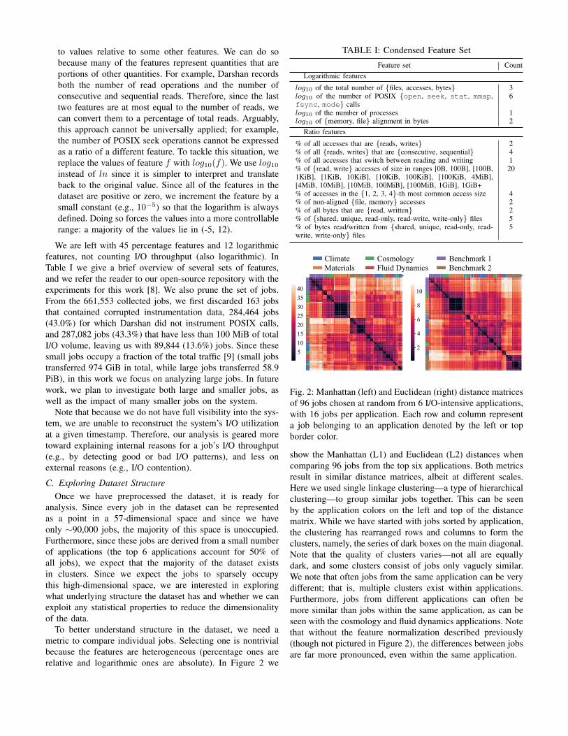
To better understand structure in the dataset, we need ametric to compare individual jobs. Selecting one is nontrivialbecause the features are heterogeneous (percentage ones arerelative and logarithmic ones are absolute). In Figure 2 we

TABLE I: Condensed Feature Set

Feature set CountLogarithmic features

log10 of the total number of {files, accesses, bytes} 3log10 of the number of POSIX {open, seek, stat, mmap,fsync, mode} calls

6

log10 of the number of processes 1log10 of {memory, file} alignment in bytes 2

Ratio features

% of all accesses that are {reads, writes} 2% of all {reads, writes} that are {consecutive, sequential} 4% of all accesses that switch between reading and writing 1% of {read, write} accesses of size in ranges [0B, 100B], [100B,1KiB], [1KiB, 10KiB], [10KiB, 100KiB], [100KiB, 4MiB],[4MiB, 10MiB], [10MiB, 100MiB], [100MiB, 1GiB], 1GiB+

20

% of accesses in the {1, 2, 3, 4}-th most common access size 4% of non-aligned {file, memory} accesses 2% of all bytes that are {read, written} 2% of {shared, unique, read-only, read-write, write-only} files 5% of bytes read/written from {shared, unique, read-only, read-write, write-only} files

5

403530252015105

10

8

6

4

2

ClimateMaterials

CosmologyFluid Dynamics

Benchmark 1Benchmark 2

Fig. 2: Manhattan (left) and Euclidean (right) distance matricesof 96 jobs chosen at random from 6 I/O-intensive applications,with 16 jobs per application. Each row and column representa job belonging to an application denoted by the left or topborder color.

show the Manhattan (L1) and Euclidean (L2) distances whencomparing 96 jobs from the top six applications. Both metricsresult in similar distance matrices, albeit at different scales.Here we used single linkage clustering—a type of hierarchicalclustering—to group similar jobs together. This can be seenby the application colors on the left and top of the distancematrix. While we have started with jobs sorted by application,the clustering has rearranged rows and columns to form theclusters, namely, the series of dark boxes on the main diagonal.Note that the quality of clusters varies—not all are equallydark, and some clusters consist of jobs only vaguely similar.We note that often jobs from the same application can be verydifferent; that is, multiple clusters exist within applications.Furthermore, jobs from different applications can often bemore similar than jobs within the same application, as can beseen with the cosmology and fluid dynamics applications. Notethat without the feature normalization described previously(though not pictured in Figure 2), the differences between jobsare far more pronounced, even within the same application.

89844

10775

8831

70621

65021

1278

60293

103368204

48671

16672551

34326

1156

1145

33121

13644

1141

3937

1356

14644

1522

10989503

62264497

11088

6799

1571

3919

1001

1101

3290

1779

1170

1280 172317941203 1485

2211

Alpha:6408jobs

Beta:4827jobs

Gamma:17159jobs

Delta:11961jobs

4

5

6

7

8

9

Epsi

lon

para

met

er: t

he d

ista

nce

at w

hich

clu

ster

s mer

ge o

r spl

it

Percentage of bytes to/from read/write files < 100%? (98% accuracy) YN

Number of POSIX reads > 0? (88% accuracy) Percentage of

unique files > 25%? (100% accuracy)

YN

YN

Number of reads in 0-100 B > 0? (90% accuracy)

Y

NYN

Number of reads in 100KiB - 1MiB > 0? (94% accuracy), or

percentage of unique files < 95%?(92% accuracy)

# of R/W switches > 0? (98% accuracy)

Y

N

Fig. 3: HDBSCAN single linkage tree, pruned of clusters smaller than 1,000 jobs and of clusters clustered at ε < 3. Note thefour clusters marked Alpha to Delta. These clusters are hand-selected using this tree and are used later in the analysis.

The existence of these clusters and of clusters of varyingdensities motivated us to further explore the structure ofthe dataset. For that purpose, we used HDBSCAN [10], ahierarchical version of the DBSCAN agglomerative clusteringalgorithm. Briefly, DBSCAN works by clustering togetherpoints within a certain distance ε and connecting graphs ofthese neighboring points into larger clusters. DBSCAN ishighly sensitive to the choice of this distance parameter ε,with small values leading to many small “islands” of jobsand large values leading to the whole dataset being placedin a single cluster. HDBSCAN allows us to visualize whatthe original DBSCAN algorithm would arrive at clustering atany ε value. HDBSCAN is sensitive to a second parameter k,which controls the minimal size of clusters. As we decrease ε,clusters will periodically split; and when these smaller “child”clusters contain less than k points, their contents will be treatedas outliers. In our experiments, we use the default value ofk = 5. A small k value allows us to explore clusters withfine granularity. In Figure 3, we show HDBSCAN’s singlelinkage tree, with both color and position of nodes on the yaxis specifying the ε value at which the cluster merges andsplits. We can see that the whole dataset gets clustered ina single cluster for large ε values and that, as we decreasethe value, the cluster gets progressively split into smaller andsmaller clusters. The lines connecting the clusters specifywhich clusters get split into or merge into which, with theline thickness being proportional to the number of jobs going

to that cluster. The values in clusters specify the number ofjobs in that cluster. The number of jobs between parent andchildren clusters may not always add up; some jobs are lostas they belong to smaller clusters that we do not plot, in orderto avoid visual clutter.

Note that we have four clusters with larger circles markedAlpha, Beta, Gamma, and Delta. We have selected theseclusters for further analysis in Section V. These specificclusters were selected because they are far from each otherin the tree and hence may have very different behaviors.Additionally, we wanted to explore the impact of granularityin our analysis. That is why we have selected the cluster Delta(bottom right) to be a sub-cluster of cluster Gamma (right).Gamma contains all of the jobs in Delta, plus 5,000 other jobs.

D. Interpreting Dataset StructureWhile Figure 3 reveals the existence of a rich structure in

the dataset, it does not increase our understanding of it. To getbetter intuition about the data distribution, we perform a simpleexperiment: since every node of the HDBSCAN single linkagetree consists of a number of smaller merged clusters, we traina decision tree that predicts where each job in the cluster willend up once the cluster splits. To help interpretability, we traindecision trees only of depth 1, namely, trees with only 2 leavesand a single decision splitting the dataset. The annotations andarrows pointing to nodes in Figure 3 explain what the decisiontrees at those nodes have learned.

Right away, the clustering splits the dataset into jobs that

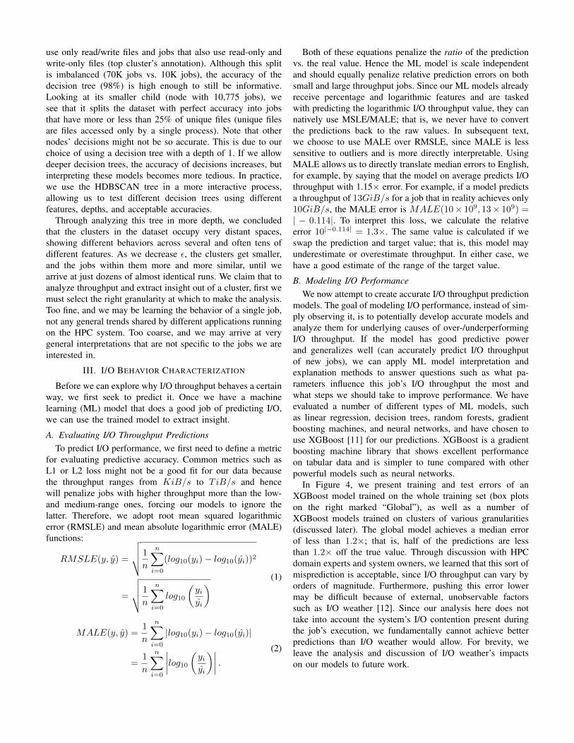
use only read/write files and jobs that also use read-only andwrite-only files (top cluster’s annotation). Although this splitis imbalanced (70K jobs vs. 10K jobs), the accuracy of thedecision tree (98%) is high enough to still be informative.Looking at its smaller child (node with 10,775 jobs), wesee that it splits the dataset with perfect accuracy into jobsthat have more or less than 25% of unique files (unique filesare files accessed only by a single process). Note that othernodes’ decisions might not be so accurate. This is due to ourchoice of using a decision tree with a depth of 1. If we allowdeeper decision trees, the accuracy of decisions increases, butinterpreting these models becomes more tedious. In practice,we use the HDBSCAN tree in a more interactive process,allowing us to test different decision trees using differentfeatures, depths, and acceptable accuracies.

Through analyzing this tree in more depth, we concludedthat the clusters in the dataset occupy very distant spaces,showing different behaviors across several and often tens ofdifferent features. As we decrease ε, the clusters get smaller,and the jobs within them more and more similar, until wearrive at just dozens of almost identical runs. We claim that toanalyze throughput and extract insight out of a cluster, first wemust select the right granularity at which to make the analysis.Too fine, and we may be learning the behavior of a single job,not any general trends shared by different applications runningon the HPC system. Too coarse, and we may arrive at verygeneral interpretations that are not specific to the jobs we areinterested in.

III. I/O BEHAVIOR CHARACTERIZATION

Before we can explore why I/O throughput behaves a certainway, we first seek to predict it. Once we have a machinelearning (ML) model that does a good job of predicting I/O,we can use the trained model to extract insight.

A. Evaluating I/O Throughput PredictionsTo predict I/O performance, we first need to define a metric

for evaluating predictive accuracy. Common metrics such asL1 or L2 loss might not be a good fit for our data becausethe throughput ranges from KiB/s to TiB/s and hencewill penalize jobs with higher throughput more than the low-and medium-range ones, forcing our models to ignore thelatter. Therefore, we adopt root mean squared logarithmicerror (RMSLE) and mean absolute logarithmic error (MALE)functions:

RMSLE(y, y) =

√√√√ 1

n

n∑i=0

(log10(yi)− log10(yi))2

=

√√√√ 1

n

n∑i=0

log10

(yiyi

) (1)

MALE(y, y) =1

n

n∑i=0

|log10(yi)− log10(yi)|

=1

n

n∑i=0

∣∣∣∣log10(yiyi)∣∣∣∣ .

(2)

Both of these equations penalize the ratio of the predictionvs. the real value. Hence the ML model is scale independentand should equally penalize relative prediction errors on bothsmall and large throughput jobs. Since our ML models alreadyreceive percentage and logarithmic features and are taskedwith predicting the logarithmic I/O throughput value, they cannatively use MSLE/MALE; that is, we never have to convertthe predictions back to the raw values. In subsequent text,we choose to use MALE over RMSLE, since MALE is lesssensitive to outliers and is more directly interpretable. UsingMALE allows us to directly translate median errors to English,for example, by saying that the model on average predicts I/Othroughput with 1.15× error. For example, if a model predictsa throughput of 13GiB/s for a job that in reality achieves only10GiB/s, the MALE error is MALE(10× 109, 13× 109) =| − 0.114|. To interpret this loss, we calculate the relativeerror 10|−0.114| = 1.3×. The same value is calculated if weswap the prediction and target value; that is, this model mayunderestimate or overestimate throughput. In either case, wehave a good estimate of the range of the target value.

B. Modeling I/O PerformanceWe now attempt to create accurate I/O throughput prediction

models. The goal of modeling I/O performance, instead of sim-ply observing it, is to potentially develop accurate models andanalyze them for underlying causes of over-/underperformingI/O throughput. If the model has good predictive powerand generalizes well (can accurately predict I/O throughputof new jobs), we can apply ML model interpretation andexplanation methods to answer questions such as what pa-rameters influence this job’s I/O throughput the most andwhat steps we should take to improve performance. We haveevaluated a number of different types of ML models, suchas linear regression, decision trees, random forests, gradientboosting machines, and neural networks, and have chosen touse XGBoost [11] for our predictions. XGBoost is a gradientboosting machine library that shows excellent performanceon tabular data and is simpler to tune compared with otherpowerful models such as neural networks.

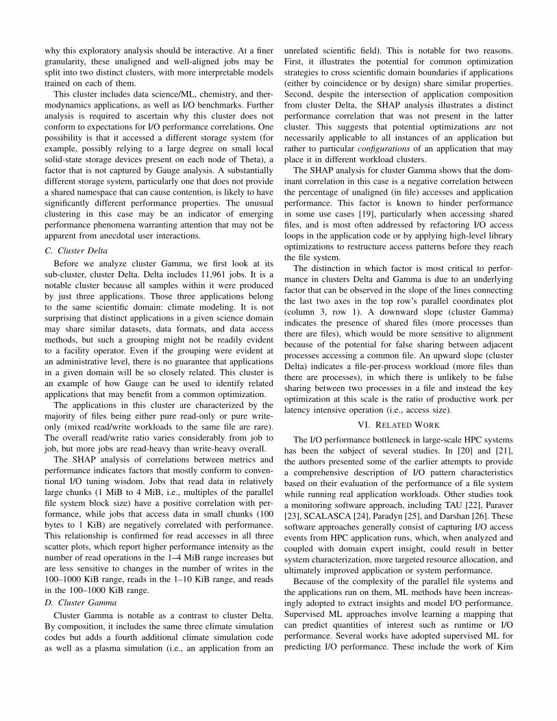
In Figure 4, we present training and test errors of anXGBoost model trained on the whole training set (box plotson the right marked “Global”), as well as a number ofXGBoost models trained on clusters of various granularities(discussed later). The global model achieves a median errorof less than 1.2×; that is, half of the predictions are lessthan 1.2× off the true value. Through discussion with HPCdomain experts and system owners, we learned that this sort ofmisprediction is acceptable, since I/O throughput can vary byorders of magnitude. Furthermore, pushing this error lowermay be difficult because of external, unobservable factorssuch as I/O weather [12]. Since our analysis here does nottake into account the system’s I/O contention present duringthe job’s execution, we fundamentally cannot achieve betterpredictions than I/O weather would allow. For brevity, weleave the analysis and discussion of I/O weather’s impactson our models to future work.

1.8×1.7×1.6×1.5×1.4×1.3×

1.2×

1.1×

1.0×

Cluster Training Errors Cluster Test ErrorsAv

erag

e Pr

edic

tion

Rat

io E

rror

1.8×1.7×1.6×1.5×1.4×1.3×

1.2×

1.1×

1.0×

Aver

age

Pred

ictio

n R

atio

Err

or

1077 267 79 10 GlobalNumber of Clusters

1077 267 79 10 GlobalNumber of Clusters

Perc

enta

ge o

f Job

s

100%

80%

60%

40%

20%

0%

Perc

enta

ge o

f Job

s100%

80%

60%

40%

20%

0%

Average Prediction Ratio Error1.0× 1.2× 1.4× 1.6× 1.8× 2.0×

Average Prediction Ratio Error1.0× 1.2× 1.4× 1.6× 1.8× 2.0×

10772677910Global

10772677910Global

Fig. 4: I/O throughput prediction results. Top row shows thetraining and test error distribution of XGBoost models trainedon clusters of various granularities. The rightmost model is asingle model trained on the whole dataset. The bottom rowshows the cumulative histogram of the above error.

Given that the global model is performing well, we seek togain insight into how the model is arriving at its predictions.To do so, we use the permutation feature importance (PFI),a statistical method [13] that evaluates the impact of everyfeature on the trained model output. The method works bytaking the trained model, selecting a feature whose importancewe want to test, and permuting its values from differentrows. This approach guarantees that the input distributionof that feature remains the same but carries no information.It permutes values instead of, for example, zeroing out thatfeature, since this may additionally hurt the model’s predictiveperformance. In Figure 5, we show the top features selectedby PFI using XGBoost predictors, on two different datasets(blue and orange). The first PFI experiment (orange lineand labels) shows feature importance of models trained ona dataset consisting of all jobs larger than 100 MiB and withfeatures from Table I. The second PFI experiment (blue lineand labels) uses the same jobs but now has ten additional time-based features: runtime; cumulative read, meta, and write timerelative to runtime; maximum read / write operation durationsrelative to runtime; and time periods between first and lastopen, close, read, and write operations relative to runtime.The figure can be interpreted as follows: For each row, theclassifier is trained on that row’s selected feature, in additionto the features from the rows above. For example, the thirdrow’s orange XGBoost predictor is trained on the total numberof bytes, read / write accesses, and percentage of reads in the[1, 10] KiB range.

First, let us look at PFI values on the original (orange)dataset, which does not contain time-based features. We briefly

analyze why these features may have been selected. We notethat important features do not necessarily imply that increasingthose feature values is beneficial for performance; in otherwords, strong negative correlations will also be treated asimportant. The total number of bytes transferred is selectedas the most important feature. The reason is that I/O-heavyapplications typically have higher throughput than smallerapplications have (Figure 1), so just from volume the modelcan narrow down throughput to two orders of magnitude.Throughput can scale with volume for a variety of reasons,for example, because larger applications being able to amortizesome of the slower operations or because more effort may bespent on optimizing more intensive applications. The numberof read and write calls likely helps the model estimate theaverage transfer size, another rough predictor of throughput.Similarly, small accesses in the 1–10 KiB range are likelycorrelated with low throughput. The number of files can beimportant, especially for applications that open one file perprocess (in Section V we analyze a cluster of such jobs).Consecutive and sequential reads and writes are preferable torandom access operations. Other features are less intuitive,such as the number of stat() calls or why PFI selectedthe percentage of the third most common access size vs. allaccesses. One of the reasons some of the later features maybe less intuitive is that XGBoost’s performance is relativelyconstant once the top 6 or 7 features are provided. If addingless important features only slightly improves model predic-tions, PFI has a high chance of incorrectly ordering features.Therefore, we should not invest too much time analyzingfeatures that are not in the top of Figure 5.

Looking at PFI results on the dataset that has additionaltime-based features, we see that just with the top four or fivefeatures the model can outperform any model trained on thedataset without time-based features. The reason is likely dueto the model learning the details of Darshan’s I/O throughputcalculation implementation. The model therefore relies heavilyon time-based features and does not utilize the rest of thedataset. This reliance prevents us from using model explana-tion techniques on it, since in our experiments the techniquesonly reinforce that time-based features are important. Hence,in order to force the model to learn relationships betweenthe I/O patterns and throughput, we remove the time-basedfeatures.

While the feature importance obtained here matches theinsights from domain experts, it does not significantly changehow we would analyze misbehaving jobs or systems. In otherwords, if we were to extract from the model advice suchas “higher I/O volume is typically correlated with higherthroughput,” “consecutive reads and writes are faster than non-consecutive,” or “unique files are preferable to shared files,”1

this advice does not help with diagnosis. We therefore focus ondeveloping more personalized, “local” advice that is applicableonly to a specific family or cluster of jobs. By trying to detect

1In Darshan, unique files are files that are accessed only by a single process.If two or more processes access the same file, that file is considered shared.

motifs in parallel execution, we hope to arrive at a greaterunderstanding of a smaller subset of jobs, instead of generalunderstanding of all the jobs.

Cumulative read time

Runtime

I/O Volume

Cumulative write timeCumulative meta time

App size(nprocs)

% of read ops in 1-10 KiB

File notaligned %

Time btw. 1st and last openTime btw. 1st and last close

Max read duration

Feature Importance in Descending Order

% of read ops in 1-10 KiB

Read/Write Acesses

I/O Volume

Number of accessed filesConsecutiveread ops %

Sequentialread ops %Number ofstat() ops

% of accessesin bin 4

Consecutivewrite ops %

Sequentialwrite ops %% of write ops in 100-1000B

Average Prediction Ratio Error1.0×1.1×1.2×1.3×1.4×1.5×1.6×1.7×1.8×

Fig. 5: Permutation feature importance (PFI) [13] of XGBoostmodels on two datasets. The blue line and labels represent PFIon a dataset with time-based features, and the orange line andlabels represent PFI on a dataset without time-based features.

IV. I/O MODEL INTERPRETATION

In this section, we focus on developing local models of I/Othroughput and interpreting them. By local, we mean cluster-specific models, instead of the whole dataset. As seen inFigure 4, by using different ε values in DBSCAN clustering,we have selected several clustering granularities that result insplitting the whole dataset into different numbers of clusters.At each granularity, we split each cluster into a training and atest set, with a 70−−30 ratio. We train one XGBoost modelper cluster and predict I/O throughput on the cluster’s testset. In Figure 4, we present a box plot of the concatenatederrors of all clusters. As we can see, with higher granularitywe achieve better I/O predictions. Note that since we areevaluating the models on a different set of data from what themodel was trained on, we are confident that the model is notsimply memorizing job-throughput pairs but has generalizedwell enough. However, notice that in Figure 4 the global modeland models trained on coarse-grained clusters (red and greenbars) achieve similar performance on both the training and testsets. On the other hand, when the dataset is split into hundredsof clusters (orange and blue bars), where each of the per-cluster models is trained on a small portion of the total data,the models that have excellent performance on the trainingset have a considerably worse performance on the test set.This is evidence of overfitting, pointing to the conclusion that

for smaller clusters we should use simpler models or strongerregularization. Even with possible overfitting, however, on thetest set these small-cluster models achieve considerably betteraccuracies compared with the global model. Therefore weseek to interpret these local models. For the interpretations,we use SHapley Additive exPlanations (SHAP) [14], [15], agame theoretic approach to interpreting black-box ML models.SHAP allows us to gain insight into the impact of each featureon a per-job level, providing us with information not onlyabout which features are important but also about how theyaffect the prediction and how they react to other features.

To apply SHAP on these local models, we design aninteractive HPC job analysis tool we call Gauge. It allowssystem administrators and I/O experts to select clusters fromthe HDBSCAN tree from Figure 3 and plot each cluster’sinformation on a dashboard. In Figure 6, we present a screen-shot of Gauge’s dashboard, showing information about fourclusters, with one cluster per column. Gauge succinctly showsthe general information about each cluster in the first tworows. Note that the same clusters that were highlighted inFigure 3 are plotted here. We have selected these clustersto better illustrate behavior of dissimilar jobs and clusters atdifferent granularities (note the large difference in ε betweenthe clusters, as shown in Figure 3).

A. Gauge DashboardThe first row shows parallel plots of logarithmic features

deemed most important by I/O experts. These plots allow theuser to quickly gain insight into the cluster’s I/O throughputvolume, numbers of files, processes, and their relationships.Note the different units: we display throughput in MiB / s,volume in GiB, and the number of accesses in thousands, whilenumbers of processes and files are not modified. We selectedMiB / s, GiB, and accesses in thousands so that the values canbe plotted on the same logarithmic scale.

The second row shows another parallel plot, this time forratio features. Note that jobs within the same cluster often havesimilar percentage features but differ in logarithmic ones. Thereason is that jobs from, say, the same application may exhibitidentical behavior but, because they were run with differentinputs, show different IO volumes, throughputs, runtimes, andso forth.

The third row shows the error distribution of three MLmodels for predicting I/O throughput. The first is simply amedian predictor—its prediction is a constant, selected as themedian I/O throughput for the whole cluster. While trivial,this predictor is useful because it often outperforms otherpredictors once the cluster is very fine-grained, and it can serveas a baseline. The second classifier is a linear regression, andthe third one is XGBoost. The linear regression performs wellon medium-granularity clusters (with hundreds or thousandsof jobs), where typically only one application’s jobs exist inthe cluster and XGBoost may overfit. For anything larger,XGBoost outperforms the constant and linear predictors, ascan be seen in the third row of Figure 6.

The fourth row shows SHAP’s summary plot for the ML

R/W Ops (in 1000s)10

0

103

106

Cluster Alpha: 6418 jobs Cluster Beta: 4833 jobs

0%25%50%75%100%

Cluster Gamma: 17197 jobs Cluster Delta: 11961 jobs

Constant Linear XGBoost

2×

3×4×

10 8

I/O Volume [GB]

0%

50%

-0.5 0.0SHAP value (impact on model output)

10 2

10 4

0 1

10 2

10 5

-0.5 -0.25 0 0.25 -0.5 -0.25 0 0.25

100

103

106

100

103

106

100

103

106

0%25%50%75%100%

0%25%50%75%100%

0%25%50%75%100%

Rel

ativ

e Er

ror

1×Constant Linear XGBoost

2×

3×4×

Rel

ativ

e Er

ror

1×Constant Linear XGBoost

2×

3×4×

Rel

ativ

e Er

ror

1×Constant Linear XGBoost

2×

3×4×

Rel

ativ

e Er

ror

1×

% R/Wswitches

Sequentialread op %

% of read opsin 4-10 MiB

I/Ovolume

SHAP value (impact on model output)

# of openoperations

# of filesopened

Memory notaligned %

App size(# of processes)

File notaligned %

I/OVolume

% of read opsin 1-4 MiB

% of consectivewrite ops

% of read opsin 1-4 MiB

% if write ops in100-1000 KiB% of read ops

in 1-10 KiB% of read ops in

100-1000 KiB

SHAP value (impact on model output) SHAP value (impact on model output)

Sequ

entia

lre

ad o

p %

10 10 10 12# of open operations

10 2 10 4I/O Volume [GB]

10 10 10 12 0%% of read ops in 1-4 MiB

20%

10 2

10 5

# of

file

s ope

ned

0%

50%

100%

File

not

alig

ned

%

10 2 10 110 210 3

% o

f writ

e op

sin

100

-100

0 K

iB

0%

50%

10 1

10 2

10 3

10 8

I/O Volume [GB]10 10 10 12

10 2

10 5

10 8

I/O Volume [GB]10 10 10 12

10 2

10 5

# of open operations10 2 10 4

# of open operations10 2 10 4

10 2

10 5

10 2

10 2

10 5

10 2

I/O Volume [GB]10 10 10 12

I/O Volume [GB]10 10 10 12

10 110 210 3

10 110 210 3

0%% of read ops in 1-4 MiB

20%

0%% of read ops in 1-4 MiB

20%

10 1

10 2

10 3

10 1

10 2

10 3

% o

f rea

d op

sin

4-1

0 M

iB

0%

50%

% R

/Wsw

itche

s

0%

50%

100%

0%

50%

100%

Mem

ory

not

alig

ned

%

10 2

10 4

App

size

(# o

f pro

cess

es)

0%

25%

50%

% o

f rea

d op

sin

1-4

MiB

0%

50%

100%

% o

f con

sect

ive

writ

e op

s

0%

20%%

of r

ead

ops

in 1

-10

KiB

0%

25%

50%

% o

f rea

d op

s in

100-

1000

KiB

Throughput [MB/s]

I/O Volume [G

B]

Runtime [s]

App size (nprocs)

R/W Ops (in 1000s)

Throughput [MB/s]

I/O Volume [G

B]

Runtime [s]

App size (nprocs)

Files (count)

R/W Ops (in 1000s)

Throughput [MB/s]

I/O Volume [G

B]

Runtime [s]

App size (nprocs)

Files (count)

R/W Ops (in 1000s)

Throughput [MB/s]

I/O Volume [G

B]

Runtime [s]

App size (nprocs)

Files (count)

Read accesses

Read-only files

Read/write file

s

Write-only file

s

Unique files

Read accesses

Read-only files

Read/write file

s

Write-only file

s

Unique files

Read accesses

Read-only files

Read/write file

s

Write-only file

s

Unique files

Read accesses

Read-only files

Read/write file

s

Write-only file

s

Unique files

Files (count)

I/O th

roug

hput

I/O th

roug

hput

I/O th

roug

hput

I/O th

roug

hput

I/O th

roug

hput

I/O th

roug

hput

I/O th

roug

hput

I/O th

roug

hput

I/O th

roug

hput

I/O th

roug

hput

I/O th

roug

hput

I/O th

roug

hput

Fig. 6: The Gauge Dashboard. The first and second rows show parallel coordinate plots of the logarithmic and percentagefeatures for four different clusters. The third row shows the performance of three different ML models trained on each cluster.The fourth row shows the SHAP summary plot for each of the clusters. The last three rows show scatter plots of featuresselected by SHAP, with the color indicating the I/O throughput.

models. These graphs should be interpreted as follows, Thereexist four rows per plot (though this is parameterizable), andeach row represents a feature. Red markers correspond tojobs with higher values and blue markers to lower values ofthat feature. The position of these markers indicates SHAP’spredicted impact of the feature on the model’s prediction.Markers on the right indicate that that job’s feature has apositive impact on predicted I/O throughput, and markers on

the left indicate that the impact is negative. As an example,the first column’s “Data volume row” has red markers (highvalues) on the right, indicating that higher data volume resultsin higher throughput for that cluster. Alternatively, the “% ROps 1–10 KiB” row in the fourth column has red markers onthe left. Thee mean that larger numbers of reads in the [1–10]KiB range result in decreased I/O throughput. Note that thescale allows us to compare the impact of different features on

I/O throughput. This is further analyzed in Section V.Rows five, six, and seven show scatter plots of different

features, colored with I/O throughput. The top feature accord-ing to SHAP is used for the x axis on all three scatter plots,while for the three y axes we use the second, third, and fourthmost important features, respectively. These scatter plots areuseful for getting a better understanding of any correlationsor relationships between features. For example, looking at thebottom three plots in the second column (cluster Beta) we canimmediately spot a linear relationship between the numberof open() operations and the number of files accessed, aswell as the number of processes. Gauge supports increasingthe numbers of SHAP features and scatter plots, as well asusing other types of plots such as correlation matrices showingfeature correlations, but these are not shown because of spaceconstraints.

Note that Gauge is an interactive tool. The user is expectedto explore different clustering granularities (perhaps arounda certain job or application) and different cluster sizes, an-alyze ML models at those granularities, compare local andglobal patterns, and explore the (often nonlinear) relationshipbetween the features using the scatter plots. Next, we providea case study using Gauge to analyze jobs from ALCF’s Thetasupercomputer.

V. CASE STUDIES

The conventional approach to I/O performance analysis inthe context of user/facility interactions is to work collabora-tively with individual users to address specific concerns or im-prove the productivity of high-profile applications. This hands-on focus has proven effective in numerous examples [16]–[18]but fails to capitalize on the potential of guidance derived frombroader contextual analysis:

• Does a given application conform to a contemporary I/Omotif at this facility that is amenable to known optimiza-tions?

• Would novel improvements to this application likely beapplicable to other production applications?

• Is this I/O motif widespread enough to warrant strategicadjustments to provisioning or procurement?

• Beyond ad hoc user feedback, how can administratorsallocate limited support resources for maximum impact?

In this section we focus on four candidate clusters identifiedusing Gauge to illustrate how its capabilities could impactproduction workloads observed on the Theta system. Theclusters are named Alpha to Delta and correspond to thelarge nodes with the same names in Figure 3 and columnsin Figure 6.

A. Cluster AlphaCluster Alpha is notable because it goes against common

access pattern expectations in that it is dominated by jobsthat perform read/write access to almost all files. There arefew pure read-only or write-only files. Read/write access to asingle file could be caused by out-of-core computations, butin this case we see a different cause. The two most common

codes in this cluster are an I/O benchmark application and adata science/ML application.

I/O benchmarks generally measure performance as theelapsed time needed to write a file (or files) and then thesubsequent elapsed time needed to read it back. Its prominentpresence in an unguided analysis of production I/O activity isnot directly relevant to scientific productivity, but it may helpa facility operator better understand the impact of performancemeasurement on the system.

The second most common code in this cluster is a datascience/ML application, which is a relatively new type ofworkload for HPC systems. Its presence and the fact that it hasa pointedly different access pattern from other clusters couldpotentially help inform strategic provisioning or procurementdecisions that are more responsive to the mix of productionapplications running at a facility, for example, by providingmore storage resources that are optimized for that particularworkload.

The SHAP analysis shows a correlation between perfor-mance and the number of times that the job alternates betweenread and write access. This is not an intuitive correlation atfirst glance, but it may indirectly indicate applications thatbenefit most from caching of recently accessed data, whichis also an indicator of potential procurement optimizations byproviding burst buffer resources to such applications. Othercorrelations indicate positive associations with data volume(which can amortize startup and metadata costs), read accesssize, and sequential property of accesses.

The third scatter plot (first column, seventh row) indicatesthat increased data volumes improve performance regardlessof how frequently applications switch between read and writeaccess patterns.

B. Cluster BetaCluster Beta is a notable case study because it does not

conform to conventional I/O tuning expectations in the SHAPanalysis. The most prominent correlations identified by Gaugeare positive correlations with the number of times that theopen() system call was invoked and the number of filesaccessed: behaviors that are not intuitively associated withimproved throughput. The first scatter plot (second column,fifth row) exhibits a diagonal pattern corresponding to jobsfor which each file was opened exactly once, but there arealso points below the diagonal that indicate jobs for whichindividual files were opened multiple times. The third corre-lation appears only in this cluster: a positive correlation withunaligned memory accesses. The second scatter plot gives anindication of why this may be misleading, however. It appearsthat the jobs are either exclusively well aligned in memoryor heavily unaligned in memory, and all of the larger jobs(and thus higher-performing jobs) fall into the latter category,producing a misleading correlation with memory alignment.Memory alignment is indeed a performance factor, but itusually is not prominent on an HPC system because of theproportionally larger impact of file alignment due to secondarystorage latency. However, this cluster is a good example of

why this exploratory analysis should be interactive. At a finergranularity, these unaligned and well-aligned jobs may besplit into two distinct clusters, with more interpretable modelstrained on each of them.

This cluster includes data science/ML, chemistry, and ther-modynamics applications, as well as I/O benchmarks. Furtheranalysis is required to ascertain why this cluster does notconform to expectations for I/O performance correlations. Onepossibility is that it accessed a different storage system (forexample, possibly relying to a large degree on small localsolid-state storage devices present on each node of Theta), afactor that is not captured by Gauge analysis. A substantiallydifferent storage system, particularly one that does not providea shared namespace that can cause contention, is likely to havesignificantly different performance properties. The unusualclustering in this case may be an indicator of emergingperformance phenomena warranting attention that may not beapparent from anecdotal user interactions.

C. Cluster DeltaBefore we analyze cluster Gamma, we first look at its

sub-cluster, cluster Delta. Delta includes 11,961 jobs. It is anotable cluster because all samples within it were producedby just three applications. Those three applications belongto the same scientific domain: climate modeling. It is notsurprising that distinct applications in a given science domainmay share similar datasets, data formats, and data accessmethods, but such a grouping might not be readily evidentto a facility operator. Even if the grouping were evident atan administrative level, there is no guarantee that applicationsin a given domain will be so closely related. This cluster isan example of how Gauge can be used to identify relatedapplications that may benefit from a common optimization.

The applications in this cluster are characterized by themajority of files being either pure read-only or pure write-only (mixed read/write workloads to the same file are rare).The overall read/write ratio varies considerably from job tojob, but more jobs are read-heavy than write-heavy overall.

The SHAP analysis of correlations between metrics andperformance indicates factors that mostly conform to conven-tional I/O tuning wisdom. Jobs that read data in relativelylarge chunks (1 MiB to 4 MiB, i.e., multiples of the parallelfile system block size) have a positive correlation with per-formance, while jobs that access data in small chunks (100bytes to 1 KiB) are negatively correlated with performance.This relationship is confirmed for read accesses in all threescatter plots, which report higher performance intensity as thenumber of read operations in the 1–4 MiB range increases butare less sensitive to changes in the number of writes in the100–1000 KiB range, reads in the 1–10 KiB range, and readsin the 100–1000 KiB range.D. Cluster Gamma

Cluster Gamma is notable as a contrast to cluster Delta.By composition, it includes the same three climate simulationcodes but adds a fourth additional climate simulation codeas well as a plasma simulation (i.e., an application from an

unrelated scientific field). This is notable for two reasons.First, it illustrates the potential for common optimizationstrategies to cross scientific domain boundaries if applications(either by coincidence or by design) share similar properties.Second, despite the intersection of application compositionfrom cluster Delta, the SHAP analysis illustrates a distinctperformance correlation that was not present in the lattercluster. This suggests that potential optimizations are notnecessarily applicable to all instances of an application butrather to particular configurations of an application that mayplace it in different workload clusters.

The SHAP analysis for cluster Gamma shows that the dom-inant correlation in this case is a negative correlation betweenthe percentage of unaligned (in file) accesses and applicationperformance. This factor is known to hinder performancein some use cases [19], particularly when accessing sharedfiles, and is most often addressed by refactoring I/O accessloops in the application code or by applying high-level libraryoptimizations to restructure access patterns before they reachthe file system.

The distinction in which factor is most critical to perfor-mance in clusters Delta and Gamma is due to an underlyingfactor that can be observed in the slope of the lines connectingthe last two axes in the top row’s parallel coordinates plot(column 3, row 1). A downward slope (cluster Gamma)indicates the presence of shared files (more processes thanthere are files), which would be more sensitive to alignmentbecause of the potential for false sharing between adjacentprocesses accessing a common file. An upward slope (clusterDelta) indicates a file-per-process workload (more files thanthere are processes), in which there is unlikely to be falsesharing between two processes in a file and instead the keyoptimization at this scale is the ratio of productive work perlatency intensive operation (i.e., access size).

VI. RELATED WORK

The I/O performance bottleneck in large-scale HPC systemshas been the subject of several studies. In [20] and [21],the authors presented some of the earlier attempts to providea comprehensive description of I/O pattern characteristicsbased on their evaluation of the performance of a file systemwhile running real application workloads. Other studies tooka monitoring software approach, including TAU [22], Paraver[23], SCALASCA [24], Paradyn [25], and Darshan [26]. Thesesoftware approaches generally consist of capturing I/O accessevents from HPC application runs, which, when analyzed andcoupled with domain expert insight, could result in bettersystem characterization, more targeted resource allocation, andultimately improved application or system performance.

Because of the complexity of the parallel file systems andthe applications run on them, ML methods have been increas-ingly adopted to extract insights and model I/O performance.Supervised ML approaches involve learning a mapping thatcan predict quantities of interest such as runtime or I/Operformance. Several works have adopted supervised ML forpredicting I/O performance. These include the work of Kim

et al. [27], who modeled key characteristics of HPC systems,such as bandwidth distribution, the ratio of request size toperformance, and idle time. Unfortunately, there is no evidenceshowing these characteristics correlate to application behavior.Dorier et al. [1] proposed the Omnisc’IO approach, whichbuilds a grammar-based model of the I/O behavior and is thenused to predict when future I/O events will happen. Madireddyet al. [3] proposed a sensitivity-based modeling approachthat leverages application and file system parameters to findpartitions in I/O performance data from benchmark applicationjobs and builds Gaussian process regression models for eachpartition to predict the I/O performance. In their follow-upwork [28], the authors adopted a neural-network-based ap-proach to build global models to predict I/O performance whileconsidering the application and file-system parameters ascategorical variables. McKenna et al. [29] manually extractedfeatures from job logs and used several ML methods to predictHPC job runtime and I/O behavior. Rodrigues et al. [30] usedfeatures extracted from log files and batch scheduler logs andpresented an ML-based tool that integrates several methods topredict resource allocation for HPC environments. Matsunagaet al. [31] presented a Predicting Query Runtime Regression(PQR2) algorithm that was used on selected features from adataset generated by running bioinformatics applications topredict execution time, memory, and disk requirements. In amore recent study, Li et al. [4] presented PIPULS, a longshort-term memory neural network implementation coupledwith a hardware prototype used for online prediction of futureI/O patterns, for applications such as flash memory solid-statedrives scheduling and garbage collection. These approachesare designed primarily for predicting the I/O performancesfor specific scenarios but provide limited insights into thesimilarities in I/O characteristics across applications and I/Obottlenecks.

Unsupervised ML approaches have been used as well to un-cover features or patterns from a dataset, instead of predictingI/O throughput. This approach was explored by [5] to discoverI/O behaviors, where k-means clustering was used to groupsimilar jobs, and identified nine access patterns representing72% of the I/O behavior. Liu et al. [32] proposed AID (Auto-matic I/O Diverter), a tool for automatic I/O characterizationand I/O scheduling. Deployed on the Titan supercomputer,AID identified I/O-heavy applications and reduced their I/Ocontention through better scheduling. Our approach uses acombination of unsupervised and supervised techniques toprovide greater model stability and robustness.

VII. FUTURE WORK

Our future work will explore three directions:Investigating external impacts on I/O performance: in thiswork, we focus primarily on internal, job-specific impacts onI/O throughput and have ignored external impacts (e.g., I/Ocontention). To explore external impacts, we plan to integratelogs from systems that measure I/O contention, as well asinclude jobs smaller than 100 MiB in our analysis, which mayallow us to better estimate I/O contention.

Improving model generalization and explanations: weplan to explore how we can further preprocess Darshan logs,as well as to investigate better models of I/O, both in orderto increase I/O throughput prediction accuracy and to arriveat models that better encapsulate I/O behavior. With betterexplainability, we hope to reduce the reliance on manualanalysis, allowing broader usage of Gauge.

Exploring sources of errors: there are four possible reasonswhy our models make errors: either the system or distributionof applications may have changed, I/O contention may affectjobs, or our models require further tuning. We hope to arrive ata better understanding of how much each of these componentscontributes to prediction error.

VIII. CONCLUSION

Writing and tuning high-performing HPC applications re-quires significant domain expertise, as well as a good under-standing of the HPC system the application will be runningon. Often, developers and system owners find that despitetheir best effort, their HPC jobs utilize only a fraction of thepromised I/O throughput. In this work, we tackled the problemof modeling application I/O performance in order to extractinsight into why applications are behaving as they do, andgeneralize this insight to larger groups of jobs. While domainexperts can analyze individual logs and give feedback on thecauses of poor I/O, such an approach is not scalable. In thiswork we set out to build tools for automated, unsupervisedgrouping of jobs with similar I/O behaviors, as well asmethods for analyzing these groups. We present Gauge: anexploratory, interactive tool for clustering jobs into a hierarchyand analyzing these groups of jobs at different granularities.Gauge consists of two parts: a clustering hierarchy of HPCjobs and a dashboard allowing a system owner or developerto gain insight into these clusters. We build this hierarchy using89,884 Darshan logs from the Argonne Leadership ComputingFacility (ALCF) Theta supercomputer, collected in the periodbetween 2017 and 2020. Using this tool and data, we ran a casestudy from the perspective of a Theta’s system administrator,showing how Gauge can detect families of applications andspot strange I/O behavior that may require further fine-tuningand optimization of these applications, hardware provisioning,or further investigation. Gauge provides novel informationthat leads to new insights, but it still requires guidance froma domain expert. Future work lies in reducing this relianceso that the techniques from Gauge can lead to more agileimprovements in the field.

ACKNOWLEDGMENTS

This work was supported by the U.S. Department of Energy,Office of Science, Advanced Scientific Computing Research,under Contract DE-AC02-06CH11357. This research usedresources of the Argonne Leadership Computing Facility atArgonne National Laboratory, which is supported by the Officeof Science of the U.S. Department of Energy under contractDE-AC02-06CH11357.

REFERENCES

[1] M. Dorier, S. Ibrahim, G. Antoniu, and R. Ross, “Omnisc’IO: agrammar-based approach to spatial and temporal I/O patterns predic-tion,” in SC’14: Proceedings of the International Conference for HighPerformance Computing, Networking, Storage and Analysis. IEEE,2014, pp. 623—634.

[2] B. Xie, Y. Huang, J. S. Chase, J. Y. Choi, S. Klasky, J. Lofstead, andS. Oral, “Predicting output performance of a petascale supercomputer,”in 26th International Symposium on High-Performance Parallel andDistributed Computing. New York: ACM, 2017, pp. 181–192.

[3] S. Madireddy, P. Balaprakash, P. Carns, R. Latham, R. Ross, S. Sny-der, and S. M. Wild, “Machine learning based parallel I/O predictivemodeling: A case study on Lustre file systems,” in High PerformanceComputing. Springer, June 2018, pp. 184–204.

[4] D. Li, Y. Wang, B. Xu, W. Li, W. Li, L. Yu, and Q. Yang, “PIPULS:Predicting I/O patterns using LSTM in storage systems,” in 2019International Conference on High Performance Big Data and IntelligentSystems (HPBD&IS). IEEE, 2019, pp. 14–21.

[5] P. J. Pavan, J. L. Bez, M. S. Serpa, F. Z. Boito, and P. O. A. Navaux,“An unsupervised learning approach for I/O behavior characterization,”in 2019 31st International Symposium on Computer Architecture andHigh Performance Computing (SBAC-PAD), 2019, pp. 33–40.

[6] S. Snyder, P. Carns, K. Harms, R. Ross, G. K. Lockwood, and N. J.Wright, “Modular HPC I/O Characterization with Darshan,” in 20165th Workshop on Extreme-Scale Programming Tools (ESPT), 2016, pp.9–17.

[7] Darshan-util installation and usage, 2020 (accessed April 22, 2020),https://www.mcs.anl.gov/research/projects/darshan/docs/darshan-util.html# darshan parser.

[8] Gauge supporting experiments, 2020 (accessed June 5, 2020), https://anonymous.4open.science/r/1c9a3777-0133-4db8-bff8-deffed0cad95/.

[9] H. Luu, M. Winslett, W. Gropp, R. Ross, P. Carns, K. Harms, M. Prabhat,S. Byna, and Y. Yao, “A multiplatform study of I/O behavior on petascalesupercomputers,” in Proceedings of the 24th International Symposiumon High-Performance Parallel and Distributed Computing, ser. HPDC’15. New York, NY, USA: Association for Computing Machinery,2015, pp. 33––44.

[10] L. McInnes, J. Healy, and S. Astels, “hdbscan: Hierarchical densitybased clustering,” The Journal of Open Source Software, vol. 2, no. 11,mar 2017.

[11] T. Chen and C. Guestrin, “XGBoost: A scalable tree boosting system,”in Proceedings of the 22nd ACM SIGKDD International Conference onKnowledge Discovery and Data Mining, ser. KDD ’16. New York, NY,USA: ACM, 2016, pp. 785–794.

[12] G. K. Lockwood, W. Yoo, S. Byna, N. J. Wright, S. Snyder, K. Harms,Z. Nault, and P. Carns, “UMAMI: A recipe for generating meaningfulmetrics through holistic i/o performance analysis,” in Proceedings ofthe 2nd Joint International Workshop on Parallel Data Storage & DataIntensive Scalable Computing Systems, ser. PDSW-DISCS ’17. NewYork, NY, USA: Association for Computing Machinery, 2017, pp. 55–60.

[13] A. Altmann, L. Tolosi, O. Sander, and T. Lengauer, “Permutationimportance: a corrected feature importance measure,” Bioinformatics,vol. 26, no. 10, pp. 1340–1347, 04 2010.

[14] S. M. Lundberg and S.-I. Lee, “A unified approach to interpreting modelpredictions,” in Advances in Neural Information Processing Systems30, I. Guyon, U. V. Luxburg, S. Bengio, H. Wallach, R. Fergus,S. Vishwanathan, and R. Garnett, Eds. Curran Associates, Inc., 2017,pp. 4765–4774.

[15] S. M. Lundberg, G. Erion, H. Chen, A. DeGrave, J. M. Prutkin,B. Nair, R. Katz, J. Himmelfarb, N. Bansal, and S.-I. Lee, “From localexplanations to global understanding with explainable AI for trees,”Nature Machine Intelligence, vol. 2, no. 1, pp. 2522–5839, 2020.

[16] R. Latham, C. Daley, W. keng Liao, K. Gao, R. Ross, A. Dubey, andA. Choudhary, “A case study for scientific I/O: improving the FLASHastrophysics code,” Computational Science & Discovery, vol. 5, no. 1,p. 015001, mar 2012.

[17] J. Kodavasal, K. Harms, P. Srivastava, S. Som, S. Quan, K. Richards,and M. Garcıa, “Development of a Stiffness-Based Chemistry Load Bal-ancing Scheme, and Optimization of Input/Output and Communication,to Enable Massively Parallel High-Fidelity Internal Combustion EngineSimulations,” Journal of Energy Resources Technology, vol. 138, no. 5,02 2016, 052203.

[18] A. Srinivasan, C. D. Sudheer, and S. Namilae, “Optimizing massivelyparallel simulations of infection spread through air-travel for policyanalysis,” in 2016 16th IEEE/ACM International Symposium on Cluster,Cloud and Grid Computing (CCGrid), May 2016, pp. 136–145.

[19] X. Zhang, K. Liu, K. Davis, and S. Jiang, “ibridge: Improving unalignedparallel file access with solid-state drives,” in 2013 IEEE 27th Interna-tional Symposium on Parallel and Distributed Processing, May 2013,pp. 381–392.

[20] A. N. Reddy and P. Banerjee, “A study of I/O behavior of perfect bench-marks on a multiprocessor,” ACM SIGARCH Computer ArchitectureNews, vol. 18, no. 2SI, pp. 312–321, 1990.

[21] P. E. Crandall, R. A. Aydt, A. A. Chien, and D. A. Reed, “Input/outputcharacteristics of scalable parallel applications,” in Proceedings of the1995 ACM/IEEE conference on Supercomputing, 1995, pp. 59–es.

[22] S. S. Shende and A. D. Malony, “The TAU parallel performance system,”The International Journal of High Performance Computing Applications,vol. 20, no. 2, pp. 287–311, 2006.

[23] V. Pillet, J. Labarta, T. Cortes, and S. Girona, “Paraver: A tool tovisualize and analyze parallel code,” in Proceedings of WoTUG-18:transputer and occam developments, vol. 44, no. 1. Citeseer, 1995,pp. 17–31.

[24] M. Geimer, F. Wolf, B. J. Wylie, E. Abraham, D. Becker, and B. Mohr,“The Scalasca performance toolset architecture,” Concurrency and Com-putation: Practice and Experience, vol. 22, no. 6, pp. 702–719, 2010.

[25] B. P. Miller, M. D. Callaghan, J. M. Cargille, J. K. Hollingsworth,R. B. Irvin, K. L. Karavanic, K. Kunchithapadam, and T. Newhall, “TheParadyn parallel performance measurement tool,” Computer, vol. 28,no. 11, pp. 37–46, 1995.

[26] P. Carns, R. Latham, R. Ross, K. Iskra, S. Lang, and K. Riley, “24/7characterization of petascale I/O workloads,” in 2009 IEEE InternationalConference on Cluster Computing and Workshops. IEEE, 2009, pp. 1–10.

[27] Y. Kim, R. Gunasekaran, G. M. Shipman, D. A. Dillow, Z. Zhang,and B. W. Settlemyer, “Workload characterization of a leadershipclass storage cluster,” in 2010 5th Petascale Data Storage Workshop(PDSW’10). IEEE, 2010, pp. 1–5.

[28] S. Madireddy, P. Balaprakash, P. Carns, R. Latham, R. Ross, S. Snyder,and S. Wild, “Modeling I/O performance variability using conditionalvariational autoencoders,” in 2018 IEEE International Conference onCluster Computing (CLUSTER). IEEE, 2018, pp. 109–113.

[29] R. McKenna, S. Herbein, A. Moody, T. Gamblin, and M. Taufer,“Machine learning predictions of runtime and IO traffic on high-endclusters,” in 2016 IEEE International Conference on Cluster Computing(CLUSTER). IEEE, 2016, pp. 255–258.

[30] E. R. Rodrigues, R. L. Cunha, M. A. Netto, and M. Spriggs, “HelpingHPC users specify job memory requirements via machine learning,” in2016 Third International Workshop on HPC User Support Tools (HUST).IEEE, 2016, pp. 6–13.

[31] A. Matsunaga and J. A. Fortes, “On the use of machine learning topredict the time and resources consumed by applications,” in 201010th IEEE/ACM International Conference on Cluster, Cloud and GridComputing. IEEE, 2010, pp. 495–504.

[32] Y. Liu, R. Gunasekaran, X. Ma, and S. S. Vazhkudai, “Server-sidelog data analytics for I/O workload characterization and coordinationon large shared storage systems,” in SC ’16: Proceedings of theInternational Conference for High Performance Computing, Networking,Storage and Analysis, 2016, pp. 819–829.

Appendix: Artifact Description/Artifact Evaluation

SUMMARY OF THE EXPERIMENTS REPORTEDWe ran 6 experiments, and each of the experiments corresponds to afigure in our paper: 1. some simple statistical plots that showed thedistribution of our data, 2. we ran permutation feature importanceexperiments to analyze XGBoost models and how they attributeimportance, 3. we ran hierarchical clustering on our dataset andhave trained predictors on individual clusters as well as the wholedataset, 4. we have ran hierarchical clustering visualizations, 5.we have plotted distance matrices of points in our dataset, and 6.we have a script that shows our tool (Gauge). Gauge runs a lot ofsmall plots, as well as training XGBoost models, and running SHAPanalysis on them (https://github.com/slundberg/shap).

ARTIFACT AVAILABILITYSoftware Artifact Availability: All author-created software arti-

facts are maintained in a public repository under an OSI-approvedlicense.

Hardware Artifact Availability: There are no author-created hard-ware artifacts.

Data Artifact Availability: All author-created data artifacts aremaintained in a public repository under an OSI-approved license.

Proprietary Artifacts: None of the associated artifacts, author-created or otherwise, are proprietary.

Author-Created or Modified Artifacts:

Persistent ID: https://anonymous.4open.science/r/1c9 ⌋

a3777-0133-4db8-bff8-deffed0cad95/↪→

Artifact name: Code supporting the submission

BASELINE EXPERIMENTAL SETUP, ANDMODIFICATIONS MADE FOR THE PAPER

Applications and versions: Python3.6

Libraries and versions: cycler==0.10.0 Cython==0.29.16 dec-orator==4.4.2 graphviz==0.13.2 hdbscan==0.8.26 joblib==0.14.1kiwisolver==1.2.0 matplotlib==3.1.2 networkx==2.4 numpy==1.18.1pandas==1.0.0 pydot==1.4.1 pyparsing==2.4.7 python-dateutil==2.8.1 pytz==2019.3 scikit-learn==0.22.1 scipy==1.4.1seaborn==0.10.0 shap==0.35.0 six==1.14.0 sklearn==0.0tqdm==4.45.0 xgboost==1.0.2

Key algorithms: HDBSCAN, SHAP, gradient boosting machines

ARTIFACT EVALUATIONVerification and validation studies: For the several machine learn-

ing models we have trained, we have always used 70-30 ratio cross-validation.

Accuracy and precision of timings: Our work does not performany timings.

Used manufactured solutions or spectral properties: /

Quantified the sensitivity of results to initial conditions and/orparameters of the computational environment: Our experiments are(for the most part) deterministic. We might have not hardcodedseeds in all of the experiments, but the only place where resultscould change is in the ML models, and all of the ML models we use(XGBoost for the most part), are robust to initial conditions.

Controls, statistics, or other steps taken to make the measurementsand analyses robust to variability and unknowns in the system. Mul-tiple of our experiments use box plots to provide an estimate ofclassifier error.