hp–pseudospectral method for solving continuous …
TRANSCRIPT

HP–PSEUDOSPECTRAL METHOD FOR SOLVING CONTINUOUS-TIME NONLINEAROPTIMAL CONTROL PROBLEMS
By
CHRISTOPHER L. DARBY
A DISSERTATION PRESENTED TO THE GRADUATE SCHOOLOF THE UNIVERSITY OF FLORIDA IN PARTIAL FULFILLMENT
OF THE REQUIREMENTS FOR THE DEGREE OFDOCTOR OF PHILOSOPHY
UNIVERSITY OF FLORIDA
2011

c© 2011 Christopher L. Darby
2

ACKNOWLEDGMENTS
I would like to thank my advisor, Dr. Anil V. Rao for guiding me through the journey
of obtaining a PhD. He has taught me to pursue excellence in all that I do. I thank him for
his guidance. I thank him for never holding me to the standard, but instead, holding me
to a higher standard.
I would also like to thank the members of my committee: Dr. William Hager,
Dr. Warren Dixon, and Dr. Norman Fitz-Coy. Dr. Hager’s experience and wisdom
has given me new perspectives on how to continue to grow as a researcher and my
conversations with Dr. Dixon and Dr. Fitz-Coy have always given me motivation to
continue my work.
I would like to also thank my fellow members of VDOL. I will never forget the times
we have shared while I have been a member of this lab. While each member of our
laboratory has enriched my life, I would specifically like to thank Divya Garg for her
ever willingness to look into and answer or ponder questions I may have regarding our
research. No matter how easy or far fetched my questions may be, she is always willing
to ponder them with me.
Finally, I would like to thank my friends, family and Christie for being there to
support and encourage me not only during my pursuit for a PhD, but, in always being
there for me for all of my pursuits in life. I know that whatever I do and wherever I go,
they will always be my constant.
3

TABLE OF CONTENTS
page
ACKNOWLEDGMENTS . . . . . . . . . . . . . . . . . . . . . . . . . . . . . . . . . . 3
LIST OF TABLES . . . . . . . . . . . . . . . . . . . . . . . . . . . . . . . . . . . . . . 7
LIST OF FIGURES . . . . . . . . . . . . . . . . . . . . . . . . . . . . . . . . . . . . . 8
ABSTRACT . . . . . . . . . . . . . . . . . . . . . . . . . . . . . . . . . . . . . . . . . 10
CHAPTER
1 INTRODUCTION . . . . . . . . . . . . . . . . . . . . . . . . . . . . . . . . . . . 12
2 MATHEMATICAL BACKGROUND . . . . . . . . . . . . . . . . . . . . . . . . . 21
2.1 Optimal Control . . . . . . . . . . . . . . . . . . . . . . . . . . . . . . . . . 212.2 Finite-Dimensional Optimization . . . . . . . . . . . . . . . . . . . . . . . 25
2.2.1 Unconstrained Minimization of a Function . . . . . . . . . . . . . . 252.2.2 Equality Constrained Minimization of a Function . . . . . . . . . . . 282.2.3 Inequality Constrained Minimization of a Function . . . . . . . . . . 302.2.4 Inequality and Equality Constrained Minimization of a Function . . 312.2.5 Finite-Dimensional Optimization As Applied to Optimal Control . . 32
2.3 Numerical Quadrature . . . . . . . . . . . . . . . . . . . . . . . . . . . . . 332.3.1 Low-Order Numerical Integrators . . . . . . . . . . . . . . . . . . . 342.3.2 Gaussian Quadrature . . . . . . . . . . . . . . . . . . . . . . . . . 352.3.3 Multiple-Interval Gaussian Quadrature . . . . . . . . . . . . . . . . 412.3.4 Summary . . . . . . . . . . . . . . . . . . . . . . . . . . . . . . . . 42
2.4 Lagrange Polynomial Approximation . . . . . . . . . . . . . . . . . . . . . 442.4.1 Single-Interval Lagrange Polynomial Approximations . . . . . . . . 442.4.2 Multiple-Interval Lagrange Polynomial Approximations . . . . . . . 482.4.3 Summary . . . . . . . . . . . . . . . . . . . . . . . . . . . . . . . . 49
3 MOTIVATION FOR AN HP–PSEUDOSPECTRAL METHOD . . . . . . . . . . . 52
3.1 Motivating Example 1: Problem with a Smooth Solution . . . . . . . . . . 523.2 Motivating Example 2: Problem with a Nonsmooth Solution . . . . . . . . 533.3 Discussion of Results . . . . . . . . . . . . . . . . . . . . . . . . . . . . . 56
4 HP–PSEUDOSPECTRAL METHOD . . . . . . . . . . . . . . . . . . . . . . . . 58
4.1 Multiple-Interval Continuous-Time Optimal Control Problem Formulation . 584.2 hp-Legendre-Gauss Transcription . . . . . . . . . . . . . . . . . . . . . . . 61
4.2.1 The hp–LG Pseudospectral Transformed Adjoint System . . . . . . 654.2.2 Sparsity of the hp–LG Pseudospectral Method . . . . . . . . . . . . 70
4.3 hp–Legendre-Gauss-Radau Transcription . . . . . . . . . . . . . . . . . . 734.3.1 The hp-LGR Pseudospectral Transformed Adjoint System . . . . . 78
4

4.3.2 Sparsity of the hp–LGR Pseudospectral Method . . . . . . . . . . . 824.4 Examples . . . . . . . . . . . . . . . . . . . . . . . . . . . . . . . . . . . . 86
4.4.1 Example 1 - Problem with a Smooth Solution . . . . . . . . . . . . 874.4.2 Example 2 - Bryson-Denham Problem . . . . . . . . . . . . . . . . 90
4.4.2.1 Case 1: Location of Discontinuity Unknown . . . . . . . . 934.4.2.2 Case 2: Location of Discontinuity Known . . . . . . . . . 93
4.5 Summary . . . . . . . . . . . . . . . . . . . . . . . . . . . . . . . . . . . . 97
5 HP–MESH REFINEMENT ALGORITHMS . . . . . . . . . . . . . . . . . . . . . 100
5.1 Approximation of Errors in a Mesh Interval . . . . . . . . . . . . . . . . . . 1015.2 hp–Mesh Refinement Algorithm 1 . . . . . . . . . . . . . . . . . . . . . . . 103
5.2.1 Increasing Degree of Approximation or Subdividing . . . . . . . . . 1035.2.2 Location of Intervals or Increase of Collocation Points . . . . . . . 1055.2.3 Stopping Criteria . . . . . . . . . . . . . . . . . . . . . . . . . . . . 1065.2.4 hp–Mesh Refinement Algorithm 1 . . . . . . . . . . . . . . . . . . . 106
5.3 hp–Mesh Refinement Algorithm 2 . . . . . . . . . . . . . . . . . . . . . . . 1075.3.1 Increasing Degree of Approximation or Subdividing . . . . . . . . . 1075.3.2 Increase in Polynomial Degree in Interval k . . . . . . . . . . . . . 1085.3.3 Determination of Number and Placement of New Mesh Points . . . 108
5.4 hp–Mesh Refinement Algorithm 2 . . . . . . . . . . . . . . . . . . . . . . . 109
6 EXAMPLES . . . . . . . . . . . . . . . . . . . . . . . . . . . . . . . . . . . . . . 112
6.1 Example 1 - Motivating Example 1 . . . . . . . . . . . . . . . . . . . . . . 1136.2 Example 2 - Reusable Launch Vehicle Re-entry Trajectory . . . . . . . . . 1166.3 Example 3: Hyper-Sensitive Problem . . . . . . . . . . . . . . . . . . . . . 120
6.3.1 Solutions for tf = 50 . . . . . . . . . . . . . . . . . . . . . . . . . . 1206.3.2 Solutions for tf = 1000 . . . . . . . . . . . . . . . . . . . . . . . . . 1216.3.3 Solutions for tf = 5000 . . . . . . . . . . . . . . . . . . . . . . . . . 1236.3.4 Summary of Example 6.3 . . . . . . . . . . . . . . . . . . . . . . . 124
6.4 Example 4: Motivating Example 2 . . . . . . . . . . . . . . . . . . . . . . 1286.5 Example 5: Minimum Time-to-Climb of a Supersonic Aircraft . . . . . . . 1306.6 Discussion of Results . . . . . . . . . . . . . . . . . . . . . . . . . . . . . 134
7 AEROASSISTED ORBITAL INCLINATION CHANGE MANEUVER . . . . . . . 138
7.1 Equations of Motion . . . . . . . . . . . . . . . . . . . . . . . . . . . . . . 1397.1.1 Constraints On the Motion of the Vehicle . . . . . . . . . . . . . . . 140
7.1.1.1 Initial and final conditions . . . . . . . . . . . . . . . . . . 1417.1.1.2 Interior point constraints . . . . . . . . . . . . . . . . . . . 1417.1.1.3 Vehicle path constraints . . . . . . . . . . . . . . . . . . . 142
7.1.2 Trajectory Event Sequence . . . . . . . . . . . . . . . . . . . . . . 1427.1.3 Performance Index . . . . . . . . . . . . . . . . . . . . . . . . . . . 143
7.2 Re-Formulation of Problem . . . . . . . . . . . . . . . . . . . . . . . . . . 1457.3 Optimal Control Problem . . . . . . . . . . . . . . . . . . . . . . . . . . . . 1467.4 All-Propulsive Inclination Change Maneuvers . . . . . . . . . . . . . . . . 147
5
7.5 Results . . . . . . . . . . . . . . . . . . . . . . . . . . . . . . . . . . . . . 1477.5.1 Unconstrained Heating Rate . . . . . . . . . . . . . . . . . . . . . . 1497.5.2 Constrained Heating Rate . . . . . . . . . . . . . . . . . . . . . . . 1537.5.3 Optimal Trajectory Structure . . . . . . . . . . . . . . . . . . . . . . 153
7.6 Discussion . . . . . . . . . . . . . . . . . . . . . . . . . . . . . . . . . . . 1597.7 Conclusions . . . . . . . . . . . . . . . . . . . . . . . . . . . . . . . . . . . 161
8 CONCLUSIONS . . . . . . . . . . . . . . . . . . . . . . . . . . . . . . . . . . . 162
8.1 Dissertation Summary . . . . . . . . . . . . . . . . . . . . . . . . . . . . . 1628.2 Future Work . . . . . . . . . . . . . . . . . . . . . . . . . . . . . . . . . . . 164
8.2.1 Continued Work on Mesh Refinement . . . . . . . . . . . . . . . . 1648.2.2 Discontinuous Costate . . . . . . . . . . . . . . . . . . . . . . . . . 165
REFERENCES . . . . . . . . . . . . . . . . . . . . . . . . . . . . . . . . . . . . . . . 166
BIOGRAPHICAL SKETCH . . . . . . . . . . . . . . . . . . . . . . . . . . . . . . . . 173
6
LIST OF TABLES
Table page
3-1 Matrix Density and CPU Time for p– and h–LGR Methods for Example 2. . . . 57
6-1 Initial Grid used in Example 6.1 . . . . . . . . . . . . . . . . . . . . . . . . . . . 114
6-2 Summary of Accuracy and Speed for Example 6.1 . . . . . . . . . . . . . . . . 115
6-3 Initial Grid used in Example 6.2 . . . . . . . . . . . . . . . . . . . . . . . . . . . 119
6-4 Summary of Accuracy and Speed for Example 6.2 . . . . . . . . . . . . . . . . 119
6-5 Initial Grid used in Example 6.3.1 . . . . . . . . . . . . . . . . . . . . . . . . . . 121
6-6 Summary of Accuracy and Speed for Example 6.3.1 . . . . . . . . . . . . . . . 121
6-7 Initial Grid used in Example 6.3.2 . . . . . . . . . . . . . . . . . . . . . . . . . . 123
6-8 Summary of Accuracy and Speed for Example 6.3.2 . . . . . . . . . . . . . . . 124
6-9 Initial Grid used in Example 6.3.3 . . . . . . . . . . . . . . . . . . . . . . . . . . 124
6-10 Summary of Accuracy and Speed for Example 6.3.3 . . . . . . . . . . . . . . . 127
6-11 Initial Grid used in Example 6.4 . . . . . . . . . . . . . . . . . . . . . . . . . . . 130
6-12 Summary of Accuracy and Speed for Example 6.4 . . . . . . . . . . . . . . . . 130
6-13 Initial Grid used in Example 6.5 . . . . . . . . . . . . . . . . . . . . . . . . . . . 133
6-14 Summary of Accuracy and Speed for Example 6.5 . . . . . . . . . . . . . . . . 134
7-1 Physical and Aerodynamic Constants. . . . . . . . . . . . . . . . . . . . . . . . 140
7

LIST OF FIGURES
Figure page
2-1 An Extremal Curve x∗(t) and a Comparison Curve x(t). . . . . . . . . . . . . . 23
2-2 eτ vs. τ and a Three Interval Trapezoid Rule Approximation. . . . . . . . . . . . 34
2-3 Error vs. Number of Intervals for Trapezoid Rule Approximation of Eq. (2-66). . 35
2-4 Legendre-Gauss Points Distribution. . . . . . . . . . . . . . . . . . . . . . . . . 39
2-5 Legendre-Gauss-Radau Points Distribution. . . . . . . . . . . . . . . . . . . . . 40
2-6 Error vs. Number of LG Points for Approximation of Eq. (2-66). . . . . . . . . . 41
2-7 Error vs. Number of LG or LGR Points for Approximation of Eq. (2-66) . . . . . 43
2-8 Approximation of f (τ) = 1/(1 + 25τ 2) Using Uniformly Spaced Support Points. 46
2-9 Approximation of f (τ) = 1/(1 + 25τ 2) Using LG Support Points. . . . . . . . . 47
2-10 Error vs. Number of Linear Approximating Intervals of Eq. (2-86) . . . . . . . . 49
2-11 Error vs. Number of Support Points for Approximating Eq. (2-86) . . . . . . . . 50
2-12 Error vs. Number of LG or LGR Intervals for Approximation of Eq. (2-86) . . . . 51
3-1 Error for p and h–LGR Approximation to Eqs. (3-1)–(3-3). . . . . . . . . . . . . 54
3-2 Error vs. Collocation Pts for p– and h–LGR Approximation to Eqs. (3-5)–(3-8) . 56
4-1 Collocation and Discretization Points by LG Methods. . . . . . . . . . . . . . . 65
4-2 Qualitative Representation of constraint Jacobian for LG points with Large Nk . 74
4-3 Qualitative Representation of constraint Jacobian for LG points with Small Nk . . 75
4-4 Collocation and Discretization Points by LGR Methods. . . . . . . . . . . . . . 79
4-5 Qualitative Representation of constraint Jacobian for LGR points with Large Nk . 85
4-6 Qualitative Representation of constraint Jacobian for LGR points with Small Nk . 86
4-7 Solution to Example 4.4.1 . . . . . . . . . . . . . . . . . . . . . . . . . . . . . . 89
4-8 Convergence Rates for LG Methods for Example 4.4.1. . . . . . . . . . . . . . 90
4-9 Convergence Rates for LGR Methods for Example 4.4.1. . . . . . . . . . . . . 91
4-10 Case 1: Convergence for LG methods for Example 4.4.2. . . . . . . . . . . . . 94
4-11 Case 1: Convergence for LGR methods for Example 4.4.2. . . . . . . . . . . . 95
8

4-12 Case 1: Solution by a Uniform h–2-Method. . . . . . . . . . . . . . . . . . . . . 96
4-13 Case 2: Convergence for p and h–3–LG and LGR Methods for Example 4.4.2 . 98
5-1 Location of Intervals if Subdivision is Chosen. . . . . . . . . . . . . . . . . . . . 105
5-2 Location of Intervals based on Curvature. . . . . . . . . . . . . . . . . . . . . . 110
6-1 State vs. Time on the Final Mesh for Example 6.2 . . . . . . . . . . . . . . . . 118
6-2 State and Control vs. Time on the Final Mesh for Example 6.3.1 . . . . . . . . 122
6-3 State and Control vs. Time on the Final Mesh for Example 6.3.3. . . . . . . . . 125
6-4 State vs. Time on the Final Mesh for Example 6.3.3. . . . . . . . . . . . . . . . 126
6-5 Control vs. Time on the Final Mesh for Example 6.4. . . . . . . . . . . . . . . . 131
6-6 State vs. Time on the Final Mesh for Example 6.5 for hp(2)–3 and ǫ = 10−4 . . . 133
7-1 Schematic of Trajectory Design for Aeroassisted Orbital Transfer Problem. . . . 144
7-2 Schematic of All-Propulsive Single Impulse and Bi-Parabolic Transfers. . . . . . 148
7-3 ∆Vmin, vs. if , and m(tf )/m0 vs. n. . . . . . . . . . . . . . . . . . . . . . . . . . 150
7-4 ∆V1, ∆V2, ∆V3, and ∆VD Impulses vs. n. . . . . . . . . . . . . . . . . . . . . . . 151
7-5 Change in i by Atmosphere, ∆iaero, and transfer time, T , vs. n for Q =∞. . . . 152
7-6 ∆Vmin, vs. n for Various Max Heating Rates and Final Inclinations. . . . . . . . 154
7-7 m(tf )/m0, vs. n for Various Qmax, and if = (20, 40, 60, 80) deg. . . . . . . . . . 155
7-8 Smax, vs. n, for Various Qmax and if = (20, 40, 60, 80) deg. . . . . . . . . . . . . 156
7-9 h vs. v , Q vs. t, and h vs. γ for if = 40-deg. . . . . . . . . . . . . . . . . . . . . 157
7-10 α and σ vs. t for n = 1 and if = 40 deg. . . . . . . . . . . . . . . . . . . . . . . 158
7-11 h vs. v for n = (1, 2, 3, 4) and if = 40 deg and Qmax = 400 (W/cm2). . . . . . . . 159
7-12 Q, vs. t for n = (1, 2, 3, 4), if = 40 deg and Qmax = 400 (W/cm2). . . . . . . . . 160
9

Abstract of Dissertation Presented to the Graduate Schoolof the University of Florida in Partial Fulfillment of theRequirements for the Degree of Doctor of Philosophy
HP–PSEUDOSPECTRAL METHOD FOR SOLVING CONTINUOUS-TIME NONLINEAROPTIMAL CONTROL PROBLEMS
By
Christopher L. Darby
May 2011
Chair: Anil V. RaoMajor: Mechanical Engineering
In this dissertation, a direct hp–pseudospectral method for approximating the
solution to nonlinear optimal control problems is proposed. The hp–pseudospectral
method utilizes a variable number of approximating intervals and variable-degree
polynomial approximations of the state within each interval. Using the hp–discretization,
the continuous-time optimal control problem is transcribed to a finite-dimensional
nonlinear programming problem (NLP). The differential-algebraic constraints of the
optimal control problem are enforced at a finite set of collocation points, where the
collocation points are either the Legendre-Gauss or Legendre-Gauss-Radau quadrature
points. These sets of points are chosen because they correspond to high-accuracy
Gaussian quadrature rules for approximating the integral of a function. Moreover,
Runge phenomenon for high-degree Lagrange polynomial approximations to the state is
avoided by using these points. The key features of the hp–method include computational
sparsity associated with low-order polynomial approximations and rapid convergence
rates associated with higher-degree polynomials approximations. Consequently, the
hp–method is both highly accurate and computationally efficient. Two hp–adaptive
algorithms are developed that demonstrate the utility of the hp–approach. The
algorithms are shown to accurately approximate the solution to general continuous-time
optimal control problems in a computationally efficient manner without a priori knowledge
of the solution structure. The hp–algorithms are compared empirically against local (h)
10
and global (p) collocation methods over a wide range of problems and are found to be
more efficient and more accurate.
The hp–pseudospectral approach developed in this research not only provides a
high-accuracy approximation to the state and control of an optimal control problem,
but also provides high-accuracy approximations to the costate of the optimal control
problem. The costate is approximated by mapping the Karush-Kuhn-Tucker (KKT)
multipliers of the NLP to the Lagrange multipliers of the continuous-time first-order
necessary conditions. It is found that if the costate is continuous, the hp–pseudospectral
method is a discrete representation of the continuous-time first-order necessary
conditions of the optimal control problem. If the costate is discontinuous, however,
and a mesh point is at the location of a discontinuity, the hp–method is an inexact
discrete representation of the continuous-time first-order necessary conditions.
The computational efficiency and accuracy of the proposed hp–method is
demonstrated on several examples ranging from problems whose solutions are smooth
to problems whose solutions are not smooth. Furthermore, a particular application
of a multiple-pass aeroassisted orbital maneuver is studied. In this application, the
minimum-fuel transfer of a small maneuverable spacecraft between two low-Earth
orbits (LEO) with an inclination change is analyzed. In the aeroassisted maneuvers,
the vehicle deorbits into the atmosphere and uses lift and drag to change its inclination.
It is found that the aeroassisted maneuvers are more fuel efficient than all-propulsive
maneuvers over a wide range of inclination changes. The examples studied in this
dissertation demonstrate the effectiveness of the hp–method.
11

CHAPTER 1INTRODUCTION
The objective of an optimal control problem is to determine the state and control
that optimize a performance index subject to dynamic constraints, boundary conditions,
and path constraints. The performance index generally represents a desired metric or
combination of metrics (e.g., fuel consumption, time, energy). Solving optimal control
problems fundamentally has its roots in the calculus of variations. Variational calculus
is used to formulate a set of necessary conditions that define extremal solutions to
an optimal control problem [1–3]. Using the calculus of variations, analytic solutions
can be found to a narrow range of simple optimal control problems. Unfortunately, in
practice, analytic solutions to general optimal control problems are difficult or impossible
to determine. Instead, such problems must be solved numerically.
Numerical methods for optimal control fall into two categories: indirect and direct
methods [4, 5]. In an indirect method, the necessary conditions from the calculus
of variations are derived and these necessary conditions result in a Hamiltonian
boundary-value problem (HBVP). Examples of indirect methods include shooting,
multiple shooting [6, 7], finite difference [8], and collocation [9, 10]. Indirect methods
are highly accurate and optimality of the continuous-time system is readily verifiable
because these methods compute extremal solutions. It is noted, however, that indirect
methods are impractical. The first disadvantage is that the necessary conditions from
the calculus of variations must be formulated which is difficult for problems of even
simple to moderate complexity. Next, the first-order optimality conditions are most often
extremely difficult to solve. Furthermore, an indirect method can only be used if good
initial guesses to the state and costate (a quantity inherent in the necessary conditions)
are provided. In particular, guesses on the costate are very difficult to generate because
the costate has no physical interpretation. Finally, for problems whose solutions have
12
active path constraints, a priori knowledge of the switching structure of the solution must
be known.
In a direct method, the optimal control problem is transcribed into a finite-dimensional
nonlinear programming problem (NLP). Many well-known and robust algorithms exist
to solve NLPs [11–13]. In a direct method, the necessary conditions from the calculus
of variations are not formulated. Moreover, direct methods do not require guesses on
the costate. In general, direct methods are not as accurate as indirect methods and
in general the first-order necessary conditions from the calculus of variations are not
satisfied.
Direct shooting [14–16] is a method which has been extensively used for launch
vehicle and orbit transfer applications [4]. A well-known computer implementation
of direct shooting is POST [17]. Successful direct shooting methods approximate
the optimal control problem using a few number of NLP variables. The success of
direct shooting methods in optimizing trajectories for launch vehicle and orbit transfer
applications is largely due to the fact that many of these problems are simple enough
that their solutions can be accurately approximated using a small number of optimization
parameters. As the number of variables used in a direct shooting method grows, the
ability to successfully use a direct shooting method rapidly declines. Furthermore,
when using a direct shooting method, the switching structure of inactive and active path
constraints must be known a priori.
Another class of a direct methods are direct collocation methods [5, 14, 18–23].
In a direct collocation method, the state is approximated using a set of trial (basis)
functions and a set of differential-algebraic constraints are enforced at a finite number
of collocation points. In contrast to indirect methods and direct shooting, a direct
collocation method does not require an a priori knowledge of the active and inactive arcs
for problems with inequality path constraints. Furthermore, direct collocation methods
are much less sensitive to initial guess than the aforementioned indirect methods
13

and direct shooting method. Some examples of computer implementations of direct
collocation methods are SOCS [24], OTIS [18], DIRCOL [25], and GPOPS [26].
In the past two decades, direct collocation methods have become more widely used
in approximating the solutions of general nonlinear optimal control problems. Typically,
direct collocation methods for optimal control are developed as h (local) methods. In an
h–method, fixed low-degree approximations are used and the problem is divided into
many subintervals. Most often, the class of Runge-Kutta methods [4, 19, 21, 27–30] are
used for h–discretization and convergence of the numerical discretization is achieved by
increasing the number of subintervals [19, 30, 31]. h–methods are utilized extensively
in approximating the solution to optimal control problems because the resulting NLP
is sparse. For a specified problem size, sparsity in the NLP greatly increases the
computational efficiency. A drawback to h–methods, however, is that convergence is at
a polynomial rate, and therefore, an excessively large number of subintervals may be
required to accurately approximate the solution. For example, in the design of an optimal
low-thrust trajectory to the moon, Ref. [32] required an approximating NLP of 211031
variables and 146285 constraints.
In contrast to h–methods, the class of direct collocation p–methods uses a
small fixed number of approximating intervals (often only a single interval is used).
Convergence to the exact solution by a p–method is achieved by increasing the
degree of the polynomial approximation in each interval. In optimal control, single
interval p–methods have been developed synonymously as pseudospectral methods
[22, 26, 33–52]. In a pseudospectral method, the collocation points are defined as
the points from highly accurate Gaussian quadratures rules. Furthermore, the basis
functions are typically Chebyshev or Lagrange polynomials. For problems whose
solutions are smooth and well-behaved, a pseudospectral method converges at an
exponential rate [53–55].
14
The most well developed pseudospectral methods are the Gauss pseudospec-
tral method (GPM) [22, 35], the Radau pseudospectral method (RPM) [38–40],
and the Lobatto pseudospectral method (LPM) [33]. In these methods, the set of
collocation points are the Legendre-Gauss (LG), Legendre-Gauss-Radau (LGR), and
the Legendre-Gauss-Lobatto (LGL) points. Furthermore, these three sets of points
are defined on the interval τ ∈ [−1, 1] and differ primarily in how the end points are
incorporated. The LG points do not include either endpoint, the LGR points include only
one end point, and the LGL points include both endpoints. Because optimal control
problems generally have boundary conditions at both the initial and terminal times,
the LGL points are the most obvious of the three sets of Gaussian quadrature points
to use. Although LGL points are the most obvious choice, recent research shows
that they may not be the most appropriate. Ref. [42] shows that the costate estimate
using LGL points tends to be noisy. In particular, it was explained in Ref. [40] that
the LGL discrete costate approximation is rank-deficient and the noisy LGL costate
approximation is due to the oscillations about the exact solution, and these oscillations
have the same behavior as the null space of the LGL approximation. Furthermore, it
was shown in Ref. [40] that not only is the LGL approximation to the costate inaccurate,
but the approximation to the control may also be inaccurate. Finally, it is noted that
when using the LG or LGR methods [22, 40], the resulting discrete approximations are
high-accuracy approximations to the solution of the optimal control problem.
While p–methods converge at an exponential rate for problems whose solutions are
smooth and well-behaved, p–methods have several limitations. First, if the solution of
a problem is not smooth, exponential convergence does not hold and the convergence
rates to the exact solution are significantly lower. Furthermore, if the solution to a
problem is smooth but has very high-order behaviors, an accurate solution is obtained
only using an unreasonably high-degree polynomial approximation. Next, the NLP
arising from a p–method is dense. Because the density of the p–method NLP is
15
high, as the degree of polynomial approximation becomes large, the NLP becomes
computationally intractable.
A third class of direct collocation methods that has not received a significant amount
of attention in approximating the solutions to optimal control problems is the class of
hp–methods. An hp–method is one in which the number of intervals, placement of
intervals, and degree of polynomial approximation in each interval is allowed to vary.
Previously, hp–methods have been used in mechanics and fluid dynamics. In particular,
Refs. [56–60] describe the mathematical properties of h, p, and hp–methods for finite
elements. It should be noted that in the period from 1975 to 1995, more than 37,000
papers related to h–methods in finite elements have been published [57]. In that same
time period, less than 100 published papers related to either p or hp–methods in finite
elements exist [57]. Therefore, historically, the vast majority of research has been in
h–methods. Some commercially available h–finite element software programs are
MSC/NASTRAN, Cosmos/M, Abaqus, Aska, Adina, and Ansys [57]. With respect to p–
and hp–methods in finite elements, some available software programs are MSC/PROBE,
Applied Structure, PHLEX and STRIPE [57].
In order to combine the benefits of h and p–methods for approximating the solution
to general optimal control problems, that is, combine the sparsity of an h–method with
the exponential convergence rate of a p–method, in this research, an hp–approach
is developed using LG and LGR points. Furthermore, because this research utilizes
collocation at points defined by Gaussian quadrature, we call these hp–pseudospectral
methods. In addition to developing hp–pseudospectral methods that provide high
accuracy approximations to the state and control, we develop high accuracy costate
estimation methods using the hp–LG and LGR methods. By providing an approximation
to the costate and not just the state and control, verification of optimality of the
original continuous-time problem may be determined from the direct hp–method. The
mapping of the Karush-Kuhn-Tucker (KKT) multipliers of the NLP to the costate of the
16
continuous-time optimal control problem are shown by first deriving the KKT conditions
of the NLP, then deriving the transformed adjoint system, and then comparing the
transformed adjoint system to the first-order necessary conditions of the continuous-time
optimal control problem. Because of the continuity constraint on the state at the mesh
points, the mapping from the KKT multipliers to the costate have two forms. If the
costate is continuous, the hp–transformed adjoint system is a discrete representation
of the continuous-time first-order necessary conditions of the optimal control problem.
If, however, the costate is discontinuous, the transformed adjoint system is no longer
a discrete representation of the continuous-time first-order necessary conditions. It
is found, however, that high levels of accuracy are still obtained in approximating the
solution to the continuous-time optimal control problem if mesh points are placed at the
location of the costate discontinuities.
To demonstrate the utility of an hp–method, two hp–mesh refinement algorithms
are presented. Previous refinement algorithms have been developed for h–methods
[30, 61] while an example of a p–mesh refinement algorithm is given in Ref. [47].
Refinement algorithms for h–methods are designed to increase the number of low-order
approximating intervals where errors are largest in approximating the solution to
the continuous-time optimal control problem. By only increasing the number of
approximating intervals where errors are large, these refinement methods increase
the computational efficiency over naive h–method approximations (i.e., a uniformly
distributed grid of approximating subintervals). Next, in the p–refinement algorithm of
Ref. [47], the algorithm increased the accuracy of the approximation, but did not address
computational efficiency. Large, dense single-interval p–approximations are used on
every iteration of the algorithm except for the final one. Only on the final iteration of
the algorithm is the approximating mesh divided. By using large, dense single-interval
p–approximations, the NLP is solved in a computationally inefficient manner.
17
In the hp–algorithms of this research, the number of intervals, width of intervals, and
polynomial degree in each interval are allowed to vary on every iteration. A two-tiered
strategy is employed to determine the locations of intervals and degree of polynomial
within each interval to achieve a specified solution accuracy. If the solution being
approximated by an interval is smooth, then the degree of approximating polynomial is
increased. Otherwise, if the solution being approximated by an interval is non-smooth,
the interval is subdivided into more low-order subintervals. The two hp–algorithms are
different because the first algorithm is more p–biased, that is, increasing the degree
of an approximating polynomial is chosen more often, and the second algorithm is
more h–biased, that is, subdivision of approximating subintervals into more low-degree
subintervals is more often chosen. Furthermore, the hp–algorithms of this research are
significantly different from the aforementioned h and p–algorithms. The hp–algorithms
of this research are different from h–algorithms because the degree of polynomial
is allowed to vary in each approximating interval. Finally, the hp–algorithms of this
research are different from the p–algorithm of Ref. [47] because the number of intervals
and location of intervals are allowed to vary on each iteration.
The contributions of this dissertation are as follows. First, hp–direct collocation
methods are described using Legendre-Gauss and Legendre-Gauss-Radau points.
If the costate is continuous, the transformed adjoint systems of the hp–LG and LGR
methods are demonstrated to be discrete representations of the continuous-time
first-order optimality conditions of an optimal control problem. As a result, high-accuracy
approximations for the state, control and costate of the solution to an optimal control
problem are obtained. Next, the hp–methods of this research combine the computational
sparsity of h–methods and the exponential convergence rates of p–methods on intervals
whose solution is sufficiently smooth. Therefore, the hp–methods result in highly efficient
and highly accurate approximations.
18
Two hp–adaptive algorithms are presented. No a priori knowledge of the solution
structure of an optimal control problem is required in order for these algorithms to
efficiently obtain highly accurate solutions. The algorithms iteratively refine the
approximating mesh using a two-tiered strategy to either increase the degree of
polynomial approximation in an interval or to subdivide the interval into more low-degree
approximating subintervals. The first algorithm presented is a p–biased algorithm,
while the second algorithm presented is an h–biased algorithm. The two algorithms
are used to solve several examples and the utility of each algorithm is demonstrated.
Furthermore, the hp–algorithms of this research are compared against each other and
with p and h–methods. It is demonstrated that the flexibility of an hp–approach adds
considerable robustness to efficiently approximating optimal control problems to a
high level of accuracy regardless of the structure of the solution of an optimal control
problem.
This dissertation is divided into the following chapters. Chapter 2 defines the
mathematical background necessary to understand the hp–methods presented. A
nonlinear optimal control problem is stated and the continuous-time first-order necessary
conditions for this problem are derived. Next, finite-dimensional optimization of a
function subject to equality and inequality constraints is examined and the KKT system
is derived. Finally, numerical integration and polynomial interpolation are examined.
Chapter 3 provides motivation for an hp–method. It is demonstrated that the method that
best approximates a general nonlinear optimal control problem is problem dependent.
Therefore, strict h or p–methods may be computationally expensive for a specific
problem type. Chapter 4 defines the hp–LG and hp–LGR discrete approximation to
the continuous-time optimal control problem. For the hp–LG and hp–LGR methods,
the KKT conditions are derived and are related to the first-order necessary conditions
of the optimal control problem. Finally, the sparsity pattern of the NLP defined by the
hp–methods of this research are examined. It is shown that the sparsity of the hp–LG
19
and LGR methods is dependent upon the degree of approximating polynomial in each
interval. Chapter 5 describes the two hp–adaptive algorithms of this dissertation. First, a
description is given on how errors are assessed in any approximating interval. Second,
the two hp–algorithms are described in detail. The first algorithm refines the mesh by
examining the relative distribution of error within each approximating interval and the
second algorithm refines the mesh by analyzing the curvature of the state. Chapter 6
presents several examples that are solved by the two hp–algorithms of this dissertation
as well as h and p–methods. It is demonstrated that the hp–algorithms are robust to
problem type and result in computationally efficient, high accuracy solutions to a wide
range of problems. In Chapter 7, a particular application of a multiple-pass aeroassisted
orbital maneuver is studied. The optimal minimum-fuel transfer of a small maneuverable
spacecraft between two low-Earth orbits with an inclination change is analyzed. Optimal
aeroglide maneuvers are compared with all-propulsive maneuvers over a wide range
of inclination change. Furthermore, a variable heating rate constraint is enforced for
the aeroglide maneuvers. It is demonstrated that an optimal aeroglide maneuver is
more fuel efficient than an all-propulsive maneuver. Finally, Chapter 8 summarizes the
contributions of this dissertation and suggests future research directions.
20
CHAPTER 2MATHEMATICAL BACKGROUND
This chapter describes the mathematical background necessary to understand the
hp–method presented in this research. The advancements of this research are founded
on optimal control theory and generating highly accurate, computationally efficient NLP
approximations to a continuous-time optimal control problem. Numerical approximation,
function approximation, and quadrature approximation theory are also foundations of
this research and are discussed in detail.
2.1 Optimal Control
The objective of an optimal control problem is to determine the state and control
that optimize a performance index subject to dynamic constraints, boundary conditions,
and path constraints. The optimal control problem studied in this research is given in
Bolza form as follows. Minimize the cost functional
J = Φ(x(t0), t0, x(tf ), tf ) +
∫ tf
t0
g(x(t),u(t))dt, (2–1)
subject to the dynamic constraints
x(t) ≡ dxdt= f(x(t),u(t)), (2–2)
the inequality path constraints
C(x(t),u(t)) ≤ 0, (2–3)
and the boundary conditions
φ(x(t0), t0, x(tf ), tf ) = 0, (2–4)
where x(t) ∈ Rn is the state, u(t) ∈ R
m is control, f : Rn×Rm −→ R
n, C : Rn×Rm −→ R
s ,
φ : Rn × R × Rn × R −→ R
q and t is time. Furthermore, Φ : Rn × R × Rn × R −→ R
is the Mayer cost and g : Rn × Rm −→ R is the Lagrangian. To determine an extremal
solution, the calculus of variations is used. The calculus of variations is used to generate
21

a set of first-order necessary conditions that must be satisfied for a candidate optimal
solution (also known as an extremal solution). An extremal solution may be a minimum,
maximum, or saddle. Second-order sufficiency conditions must be checked to verify that
an extremal solution is a minimum. The continuous-time first-order necessary conditions
for the optimal control problem defined by Eqs. (2–1)–(2–4) are now derived.
First, the constraints are adjoined to the cost functional to form an augmented cost
functional as
Ja = Φ(x(t0), t0, x(tf ), tf )−ψT
φ(x(t0), t0, x(tf ), tf ) (2–5)
+
∫ tf
t0
[g(x(t),u(t))− λT(t)(x(t)− f(x(t),u(t)))− γT(t)C(x(t),u(t))]dt,
where λ(t) is the costate and γ(t) and ψ are the Lagrange multipliers corresponding
to Eqs. (2–3), and (2–4), respectively. The first-order variation with respect to all free
variables is given as
δJa =∂Φ
∂x(t0)δx0 +
∂Φ
∂t0δt0 +
∂Φ
∂x(tf )δxf +
∂Φ
∂tfδtf (2–6)
−δψTφ−ψT ∂φ
∂x(t0)δx0 −ψ
T ∂φ
∂t0δt0 −ψ
T ∂φ
∂x(tf )δxf −ψ
T ∂φ
∂tfδtf
+((g − λT(x− f)− γTC)|t=tf )δtf − ((g − λT
(x− f)− γTC)|t=t0)δt0
+
∫ tf
t0
[
∂g
∂xδx+
∂g
∂uδu− δλ
T
(x− f) + λT ∂f∂xδx+ λ
T ∂f
∂uδu
−λTδx− δγT
C− γT ∂C∂x
δx− γT ∂C∂u
δu
]
dt.
Next, integrating by parts the term containing δx such that it can be expressed in terms
of δx(t0), δx(tf ), and δx gives
∫ tf
t0
−λTδxdt = −λT(tf )δx(tf ) + λT
(t0)δx(t0) +
∫ tf
t0
λT
δxdt. (2–7)
22

Two relationships relating δxf to δx(tf ) and δx0 to δx(t0) are given as
δx0 = δx(t0) + x(t0)δt0 (2–8)
δxf = δx(tf ) + x(tf )δtf . (2–9)
The relationships given in Eq. (2–8) and (2–9) are interpreted by examining Fig. 2-1.
In Fig. 2-1, x∗(t) represents an extremal curve and x(t) represents a neighboring
comparison curve where t0 and x0 are fixed. δx(tf ) is the difference between x∗(t) and
x(t) evaluated at tf . δxf is the difference between x∗(t) and x(t) evaluated at the end of
each curve, respectively. As can be seen in Fig. 2-1, Eq. (2–9) represents a first-order
approximation to δxf . The same result holds for free initial conditions on t0 and x0, giving
the relationship of Eq. (2–8). Substituting Eqs. (2–7), (2–8) and (2–9) into Eq. (2–6) and
Figure 2-1. An Extremal Curve x∗(t) and a Comparison Curve x(t).
23
grouping terms, the variation of Ja is given as
δJa =
(
∂Φ
∂x(t0)−ψT ∂φ
∂x(t0)+ λ
T
(t0)
)
δx0 (2–10)
+
(
∂Φ
∂x(tf )−ψT ∂φ
∂x(tf )− λT(tf )
)
δxf
−δψTφ
+
(
∂Φ
∂t0−ψT ∂φ
∂t0− g(t0)− λ
T
(t0)f(t0) + γT
(t0)C(t0)
)
δt0
+
(
∂Φ
∂tf−ψT ∂φ
∂tf+ g(tf ) + λ
T
(tf )f(tf )− γT
(tf )C(tf )
)
δtf
+
∫ tf
t0
[
(∂g
∂x+ λ
T ∂f
∂x− γT ∂C
∂x+ λ)δx+ (
∂g
∂u+ λ
T ∂f
∂u− γT ∂C
∂u)δu
−δλT(x− f)− δγT
C]
dt.
The first-order optimality conditions are formed by setting the variation of Ja equal to
zero with respect to each free variable. In order to write these conditions in a convenient
form, first, the augmented Hamiltonian is defined. Defining the augmented Hamiltonian
as
H(x(t),u(t),λ(t),γ(t)) = g(x(t),u(t))+λT
(t)f(x(t),u(t))−γT(t)C(x(t),u(t)), (2–11)
the first-order optimality conditions are then expressed as
xT
(t) =∂H
∂λ(2–12)
λT
(t) = −∂H∂x
(2–13)
0 =∂H
∂u(2–14)
λT
(t0) = − ∂Φ
∂x(t0)+ψ
T ∂φ
∂x(t0)(2–15)
λT
(tf ) =∂Φ
∂x(tf )−ψT ∂φ
∂x(tf )(2–16)
H(t0) = −ψT ∂φ∂t0+∂Φ
∂t0(2–17)
H(tf ) = ψT ∂φ
∂tf− ∂Φ
∂tf. (2–18)
24

Furthermore, using the complementary slackness condition, γ takes the value
γi(t) = 0,when Ci(x(t),u(t)) < 0, i = 1, ... , s (2–19)
γi(t) < 0,when Ci(x(t),u(t)) = 0, i = 1, ... , s. (2–20)
The negativity of γi when Ci = 0 is interpreted such that improving the cost may only
come from violating the constraint [2]. Furthermore, γi(t) = 0 when Ci < 0 states that
this constraint is inactive, and therefore, ignored. The continuous-time first-order
optimality conditions of Eqs. (2–12)–(2–20) define a set of necessary conditions
that must be satisfied for an extremal solution of an optimal control problem. The
second-order sufficiency conditions can be inspected to determine whether the extremal
solution is a minimizing solution.
2.2 Finite-Dimensional Optimization
In a direct collocation approximation of an optimal control problem, the continuous-time
optimal control problem is transcribed into a nonlinear programming problem (NLP).
While the continuous-time optimal control problem is an infinite-dimensional problem of
finding continuous-time functions that minimize a cost functional subject to differential
and algebraic constraints, an NLP is a finite-dimensional problem of finding a vector of
static parameters that minimize a cost function subject to algebraic constraints. In this
section the topics of unconstrained minimization, equality constrained minimization, and
inequality constrained minimization of a function are discussed. Moreover, an iterative
Newton method is shown for determining a minimum of a function.
2.2.1 Unconstrained Minimization of a Function
Consider the following problem of determining the minimum of a function subject to
multiple variables without any constraints. Minimize the objective function
J(x), (2–21)
25

where xT= (x1, ... , xn). For x∗ to be a locally minimizing point, the objective function
must be greater when evaluated at any neighboring point, i.e.,
J(x) > J(x∗). (2–22)
In order to develop a set of sufficient conditions defining a locally minimizing point x∗,
first, a three term Taylor series expansion about some point, x, is used to approximate
the objective function as
J(x) = J(x) + gT
(x)(x− x) + 12(x− x)TH(x)(x− x) + higher order terms (2–23)
where the gradient vector, g(x), is
g(x) ≡ ∇xJ ≡(
∂J
∂x
)T
=
∂J∂x1
∂J∂x2
...
∂J∂xn
(2–24)
and the symmetric n × n Hessian matrix is
H(x) ≡ ∇xxJ ≡∂2J
∂x2=
∂2J∂x21
∂2J∂x1∂x2
... ∂2J∂x1∂xn
∂2J∂x2∂x1
∂2J∂x22
... ∂2J∂x2∂xn
...
∂2J∂xn∂x1
∂2J∂xn∂x2
... ∂2J∂x2n
. (2–25)
For x∗ to be a local minimizing point, two conditions must be satisfied. First, a necessary
condition is that g(x∗) must be zero, i.e.,
g(x∗) = 0. (2–26)
The necessary condition by itself only defines an extremal point which can be a local
minimum, local maximum, or saddle point. In order to ensure x∗ is a local minimum, then
26
an additional condition that must be satisfied is
(x− x∗)TH(x∗)(x− x∗) > 0. (2–27)
Eqs. (2–26) and (2–27) together define sufficient conditions for a local minimum.
In order to iteratively find a minimum of the objective function, first, consider again
the approximation of Eq. (2–23) using a Taylor series expansion about some point x(i),
such that an approximation at a new point x(i+1) is given as
J(x(i+1)) ≈ J(x(i)) + g(i)T(x(i+1) − x(i)) + 12(x(i+1) − x(i))TH(i)(x(i+1) − x(i)) (2–28)
where g(i) = g(x(i)) and H(i) = H(x(i)). Next, defining the search direction, p(i+1) =
x(i+1) − x(i), the approximation to J(x(i+1)) can then be written as
J(x(i+1)) ≈ J(x(i)) + g(i)Tp(i+1) + 12p(i+1)
T
H(i)p(i+1). (2–29)
In order to find a minimum of J(x), the Taylor series expansion in Eq. (2–29) is
differentiated with respect to x(i+1) and this derivative is set to zero such that
g(i+1) = 0 = g(i) +H(i)p(i+1). (2–30)
Rearranging Eq. (2–30), the Newton search direction is given as
p(i+1) = −H(i)−1g(i). (2–31)
Finally, to ensure that the search is for a minimum and not a stationary point or a
maximum, the descent condition is enforced,
g(i)T
p(i+1) < 0. (2–32)
Eq. (2–31) is then applied iteratively from some initial guess x(i) such that a new point
x(i+1) is found. If,
J(x(i+1)) < J(x(i)), (2–33)
27

for each iteration, i , then Eq. (2–31) is applied iteratively until a minimum is found.
2.2.2 Equality Constrained Minimization of a Function
Consider finding the minimum of the objective function
J(x) (2–34)
subject to a set of m ≤ n constraints
f(x) = 0. (2–35)
Finding the minimum of an objective function subject to equality constraints uses an
approach similar to the calculus of variations approach for determining the extremal of
functionals. Define the Lagrangian as
L(x,λ) = J(x)− λTf(x) (2–36)
where λT
= (λ1, ... ,λm) are the Lagrange multipliers. Then, a necessary condition for
the minimum of the Lagrangian is that the point (x∗,λ∗) satisfies
∇xL(x∗,λ∗) = 0 (2–37)
∇λL(x∗,λ∗) = 0. (2–38)
Furthermore, the gradient of L with respect to x and λ is
∇xL = g(x)− GT(x)λ (2–39)
∇λL = −f(x) (2–40)
28

where the Jacobian matrix, G(x), is defined as
G(x) ≡ ∂f
∂x=
∂f1∂x1
∂f1∂x2
... ∂f1∂xn
∂f2∂x1
∂f2∂x2
... ∂f2∂xn
...
∂fm∂x1
∂fm∂x2
... ∂fm∂xn
. (2–41)
It is noted that at a minimum of the Lagrangian, the equality constraint of Eq. (2–35) is
satisfied. Next, this necessary condition alone does not specify a minimum, maximum or
saddle point. In order to specify a minimum, first, define the Hessian of the Lagrangian
as
HL = ∇xxL = ∇xxJ −m∑
i=1
λi∇xxfi . (2–42)
Then, a sufficient condition for a minimum is that
vTHLv > 0 (2–43)
for any vector v in the constraint tangent space.
In order to iteratively find a minimum of the Lagrangian, a two-term Taylor series
expansion of Eqs. (2–39) and (2–40) about some point (x(i),λ(i)) is equated to zero
giving
0 = g(i) − G(i)Tλ(i) +H(i)L (x(i+1) − x(i))− G(i)T
(λ(i+1) − λ(i)) (2–44)
0 = −f(i) − G(i)(x(i+1) − x(i)) (2–45)
where G(i) = G(x(i)) and H(i)L = HL(x(i)). After simplification, these equations lead to the
following linear system of equations:
H(i)L G(i)
T
G(i) 0
−p(i+1)
λ(i+1)
=
g(i)
f(i)
. (2–46)
29
It is noted that Eq. (2–46) is called the Karush-Kuhn-Tucker (KKT) system [19] which
is implemented in an NLP such as SNOPT [11]. Eq. (2–46) is solved iteratively until a
minimum to the Lagrangian is found. It is noted that Eq. (2–46) only defines an extremal
point. In order to find a locally minimizing point, Eq. (2–43) must also be satisfied. In
determining a minimum to the Lagrangian, a minimum to J(x) subject to the constraints
f(x) = 0 is found.
2.2.3 Inequality Constrained Minimization of a Function
Consider the problem of minimizing the objective function
J(x) (2–47)
subject to the inequality constraints
c(x) ≤ 0. (2–48)
Inequality constrained problems are solved by dividing the inequality constraints into a
set of active constraints, and a set of inactive constraints. At the solution x∗, some of the
constraints are satisfied as equalities, that is
ci(x∗) = 0, i ∈ A (2–49)
where A is called the active set, and some constraints are strictly satisfied, that is
ci(x∗) < 0, i ∈ A′ (2–50)
where A′ is called the inactive set.
By separating the inequality constraints into an active set and an inactive set, the
active set can be dealt with as equality constraints as described in the previous section,
and the inactive set can be ignored. The added complexity of inequality constrained
problems is in determining which set of constraints are active, and which are inactive. If
the active and inactive sets are known, an inequality constrained problem becomes an
30
equality constrained problem stated as minimize the objective function
J(x) (2–51)
subject to the constraints
ci(x) = 0, i ∈ A (2–52)
and the same methodology is applied as in the previous section to determine a
minimum.
2.2.4 Inequality and Equality Constrained Minimization of a Function
Finally, consider the problem of finding the minimum of the objective function
J(x) (2–53)
subject to the equality constraints
f(x) = 0 (2–54)
and the inequality constraints
c(x) ≤ 0. (2–55)
Define the Lagrangian as
L(x,λ,ψ(A)) = J(x)− λTf(x)−ψ(A)Tc(A)(x) (2–56)
where λ are the Lagrange multipliers with respect to the equality constraints and ψ(A)
are the Lagrange multipliers associated with the active set of inequality constraints.
Furthermore, note that ψ(A′) = 0, and therefore, the inactive set of of constraints are
ignored. A necessary condition for the minimum of the Lagrangian is that the point
(x∗,λ∗,ψ(A)∗) satisfies
∇xL(x∗,λ∗,ψ(A)∗) = 0 (2–57)
∇λL(x∗,λ∗,ψ(A)∗) = 0 (2–58)
∇ψ(A)L(x∗,λ∗,ψ(A)∗) = 0. (2–59)
31
Next, applying a two-term Taylor series approximation to the necessary conditions of
Eqs. (2–57)–(2–59) gives
0 = g(i) − G(i)Tf λ(i) − G(i)Tc(A)ψ(i)(A) +H
(i)L (x
(i+1) − x(i)) (2–60)
−G(i)Tf (λ(i+1) − λ(i))− G(i)T
c(A)(ψ(i+1)(A) −ψ(i)(A))
0 = −f(i) − G(i)f (x(i+1) − x(i)) (2–61)
0 = −c(i)(A) − G(i)c(A)(x(i+1) − x(i)) (2–62)
where Gf(x) is the Jacobian with respect to the equality constraints and Gc(A)(x) is the
Jacobian with respect to the active inequality constraints. Furthermore, HL in this case is
defined as
HL = ∇2xxL = ∇2xxJ −m∑
i=1
λi∇2xxfi −q
∑
i=1
ψ(A)i ∇2xxc (A)i (2–63)
where q is the number of active inequality constraints. Therefore, the resulting KKT
system is given as
H(i)L G
(i)T
f G(i)T
c(A)
G(i)f 0 0
G(i)
c(A)0 0
−p(i+1)
λ(i+1)
ψ(i+1)(A)
=
g(i)
f(i)
c(i)(A)
. (2–64)
For the problem of minimizing an objective function subject to equality and inequality
constraints, the KKT system of Eq. (2–64) is solved iteratively such that a minimizing
points (x∗,λ∗,ψ(A)∗) is found. Again it is noted that for (x∗,λ∗,ψ(A)∗) to be a minimizing
point, Eq. (2–43) must be satisfied as well.
2.2.5 Finite-Dimensional Optimization As Applied to Optim al Control
NLPs are used to approximate a continuous-time optimal control problem by a direct
collocation method such that the finite-dimensional optimization techniques of Section
2.2 can be used and the difficult problem of solving the continuous-time first-order
necessary conditions is avoided. The KKT system of Eq. (2–46) or Eq. (2–64) is solved
iteratively until a minimum is found for the objective function. There are two primary
32
considerations in constructing NLPs that approximate continuous-time optimal control
problems. The first and most important consideration is if the discrete approximation will
provide an accurate approximation to the solution of a continuous-time optimal control
problem. The second consideration is that if the discrete approximation is accurately
approximating the solution of a continuous-time optimal control problem, is it also a
computationally efficient problem to solve. If the KKT system of Eq. (2–46) or Eq. (2–64)
grows large, that is, the number of variables and / or number of constraints is large,
iteratively solving Eq. (2–46) or Eq. (2–64) will become excessively computationally
expensive. Furthermore, if the Hessian or Jacobian matrices are very dense, that
is, a large number of their entries are non-zero, then again, the problem will become
excessively computationally expensive. In order to maintain computational tractability
of the NLP, the KKT system should be constructed to be simultaneously as small and
sparse as possible while providing an accurate approximation of the continuous-time
optimal control problem.
2.3 Numerical Quadrature
Two concepts are important in constructing the discretized finite-dimensional
optimization problem of this research from the continuous-time optimal control problem.
These two concepts are numerical quadrature (numerical integration) and polynomial
interpolation. Numerical quadrature can generally be described as sampling an
integrand at a finite number of points and using a weighted sum of these points to
approximate the integral. In this section, first, low-order numerical integrators are briefly
discussed. Next, Gaussian quadrature rules are presented and it is shown that the
quadrature rules associated with the LG points are the most accurate quadrature rules.
Moreover, the quadrature rules associated with the LGR points are the second most
accurate quadrature rules.
33
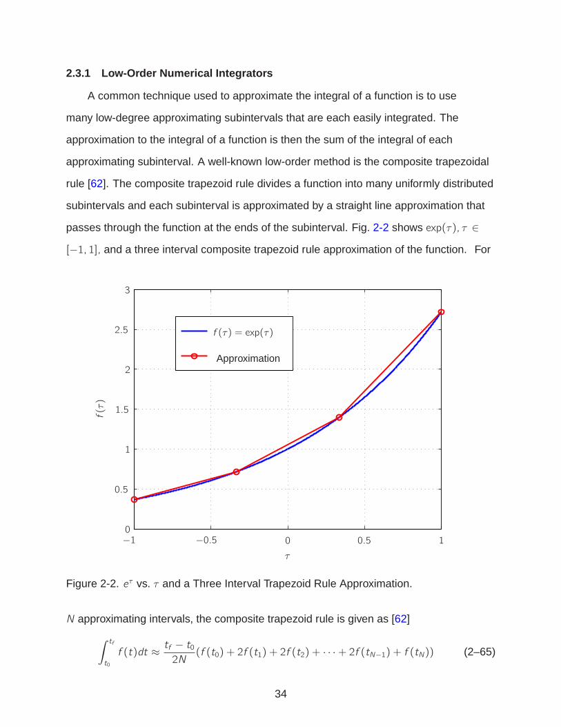
2.3.1 Low-Order Numerical Integrators
A common technique used to approximate the integral of a function is to use
many low-degree approximating subintervals that are each easily integrated. The
approximation to the integral of a function is then the sum of the integral of each
approximating subinterval. A well-known low-order method is the composite trapezoidal
rule [62]. The composite trapezoid rule divides a function into many uniformly distributed
subintervals and each subinterval is approximated by a straight line approximation that
passes through the function at the ends of the subinterval. Fig. 2-2 shows exp(τ), τ ∈
[−1, 1], and a three interval composite trapezoid rule approximation of the function. For
f (τ) = exp(τ)
f(τ)
Approximation
τ
00
1.5
2
2.5
3
−1 −0.5
0.5
0.5
1
1
Figure 2-2. eτ vs. τ and a Three Interval Trapezoid Rule Approximation.
N approximating intervals, the composite trapezoid rule is given as [62]
∫ tf
t0
f (t)dt ≈ tf − t02N
(f (t0) + 2f (t1) + 2f (t2) + · · ·+ 2f (tN−1) + f (tN)) (2–65)
34
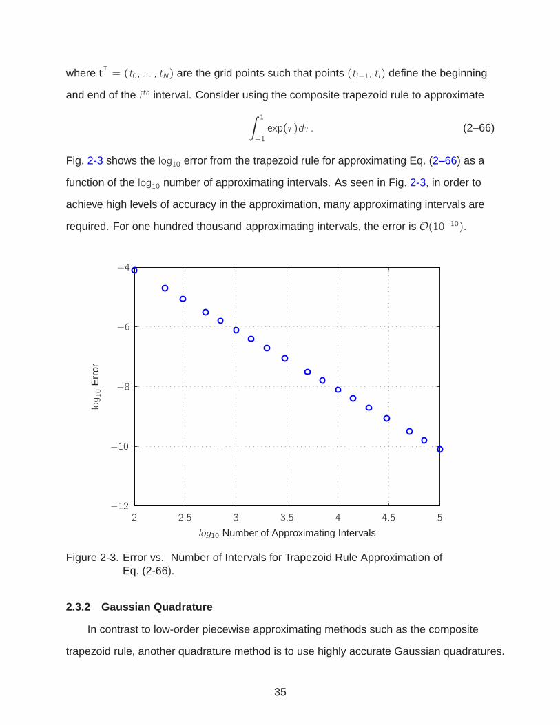
where tT= (t0, ... , tN) are the grid points such that points (ti−1, ti) define the beginning
and end of the i th interval. Consider using the composite trapezoid rule to approximate
∫ 1
−1
exp(τ)dτ . (2–66)
Fig. 2-3 shows the log10 error from the trapezoid rule for approximating Eq. (2–66) as a
function of the log10 number of approximating intervals. As seen in Fig. 2-3, in order to
achieve high levels of accuracy in the approximation, many approximating intervals are
required. For one hundred thousand approximating intervals, the error is O(10−10).
2 2.5 3 4 5
−4
−6
−8
−10
−12
log10
Err
or
log10 Number of Approximating Intervals
n
3.5 4.5
Figure 2-3. Error vs. Number of Intervals for Trapezoid Rule Approximation ofEq. (2-66).
2.3.2 Gaussian Quadrature
In contrast to low-order piecewise approximating methods such as the composite
trapezoid rule, another quadrature method is to use highly accurate Gaussian quadratures.
35
In using an n point Gaussian quadrature, two quantities must be specified for each
point, namely, the location of the point, and, a weighting factor multiplying the value
of the function evaluated at this point. The three sets of points defined by Gaussian
quadrature are the Legendre-Gauss (LG), Legendre-Gauss-Radau (LGR), and the
Legendre-Gauss-Lobatto (LGL) points. For the LG points, the points are free to be
placed anywhere on the domain τ ∈ [−1, 1], for the LGR, one end point is fixed at
τ1 = −1 and for the LGL, both end points are fixed at (τ1, τn) = (−1, 1). The goal of a
Gaussian quadrature is to construct an n point approximation
n∑
i=1
wi fi (2–67)
where wi is the quadrature weight associated with point τi and fi = f (τi), such that
the approximation in Eq. (2–67) is exact for polynomials f (τ) of as large a degree
as possible [62]. Let En(f ) be the error between the integral of f (τ) and an n point
quadrature approximation to the integral of f (τ), that is,
En(f ) =
∫ 1
−1
f (τ)dτ −n
∑
i=1
wi fi . (2–68)
First, it is noted that for
En(a0 + a1τ + · · ·+ amτm) = a0En(1) + a1En(τ) + · · ·+ amEn(τm) (2–69)
that En(f ) = 0 for every polynomial of degree ≤ m if and only if
En(τi) = 0, (i = 0, 1, ... ,m). (2–70)
Next, consider the construction of a quadrature to be exact for a polynomial of as
large a degree as possible while requiring τ1 = −1 (that is, consider the construction
of the LGR points). Two examples are provided to demonstrate how this quadrature is
constructed.
36
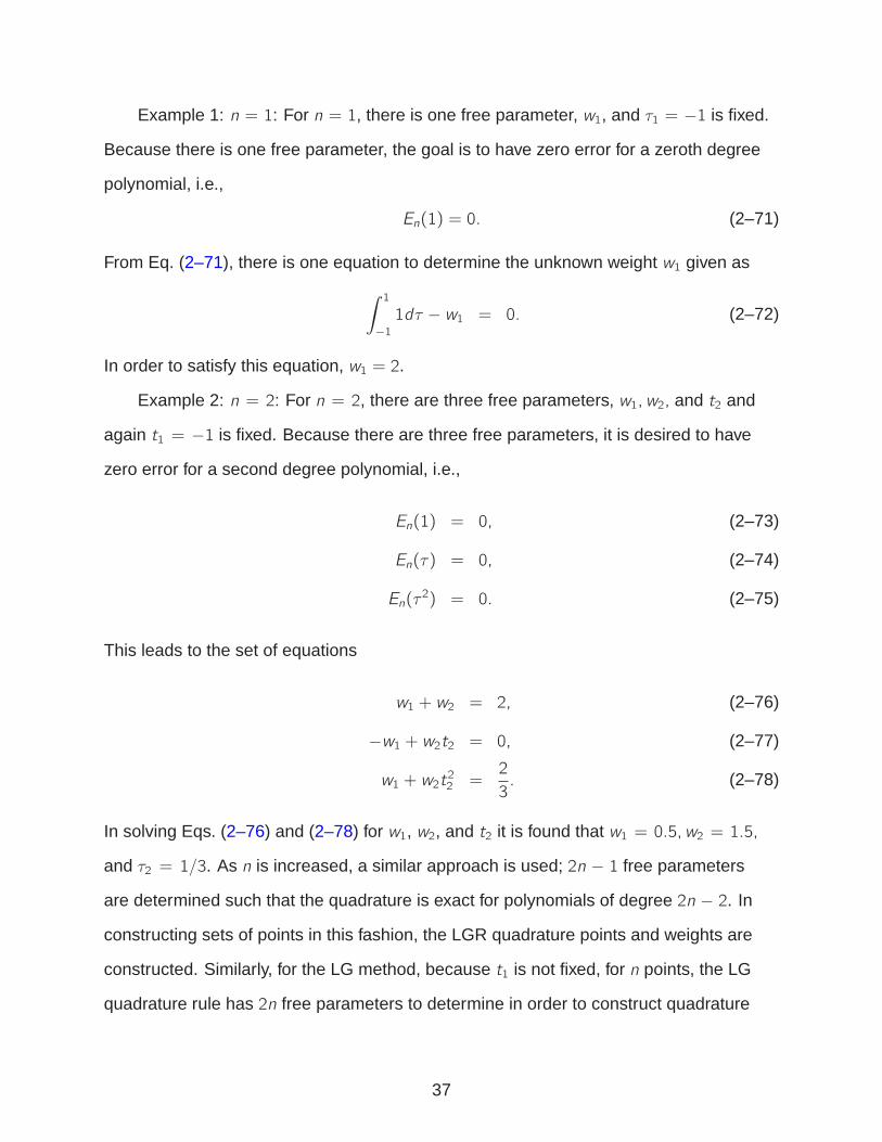
Example 1: n = 1: For n = 1, there is one free parameter, w1, and τ1 = −1 is fixed.
Because there is one free parameter, the goal is to have zero error for a zeroth degree
polynomial, i.e.,
En(1) = 0. (2–71)
From Eq. (2–71), there is one equation to determine the unknown weight w1 given as
∫ 1
−1
1dτ − w1 = 0. (2–72)
In order to satisfy this equation, w1 = 2.
Example 2: n = 2: For n = 2, there are three free parameters, w1,w2, and t2 and
again t1 = −1 is fixed. Because there are three free parameters, it is desired to have
zero error for a second degree polynomial, i.e.,
En(1) = 0, (2–73)
En(τ) = 0, (2–74)
En(τ2) = 0. (2–75)
This leads to the set of equations
w1 + w2 = 2, (2–76)
−w1 + w2t2 = 0, (2–77)
w1 + w2t22 =
2
3. (2–78)
In solving Eqs. (2–76) and (2–78) for w1, w2, and t2 it is found that w1 = 0.5,w2 = 1.5,
and τ2 = 1/3. As n is increased, a similar approach is used; 2n − 1 free parameters
are determined such that the quadrature is exact for polynomials of degree 2n − 2. In
constructing sets of points in this fashion, the LGR quadrature points and weights are
constructed. Similarly, for the LG method, because t1 is not fixed, for n points, the LG
quadrature rule has 2n free parameters to determine in order to construct quadrature
37
approximations accurate for functions of degree up to and including 2n − 1. As a
result, for a given number of points, the LG method provides the highest accuracy
quadrature approximation of any quadrature rules, while the LGR method provides the
next highest precision. The LGL quadrature rule, for n points, has 2n− 2 free parameters
and are accurate for polynomials of degree up to and including 2n − 3. It should be
noted once again that the LG and LGR points are studied in this research because the
LGL points have previously been demonstrated to result in inaccurate pseudospectral
approximations to continuous-time optimal control problem [40, 42]. As n becomes
large, determining the LG, LGR, or LGL points and weights becomes increasingly
more difficult by the method exemplified in the aforementioned two examples. The
resulting set of equations are nonlinear and their solutions are not obvious. Fortunately,
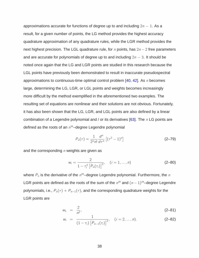
it has also been shown that the LG, LGR, and LGL points are also defined by a linear
combination of a Legendre polynomial and / or its derivatives [63]. The n LG points are
defined as the roots of an nth–degree Legendre polynomial
Pn(τ) =1
2nn!
dn
dτ n[
(τ 2 − 1)n]
(2–79)
and the corresponding n weights are given as
wi =2
1− τ 2i[
Pn(τi)]2, (i = 1, ... , n) (2–80)
where Pn is the derivative of the nth–degree Legendre polynomial. Furthermore, the n
LGR points are defined as the roots of the sum of the nth and (n− 1)th–degree Legendre
polynomials, i.e., Pn(τ) + Pn−1(τ), and the corresponding quadrature weights for the
LGR points are
w1 =2
n2, (2–81)
wi =1
(1− τi)[
Pn−1(τi)]2, (i = 2, ... , n). (2–82)
38
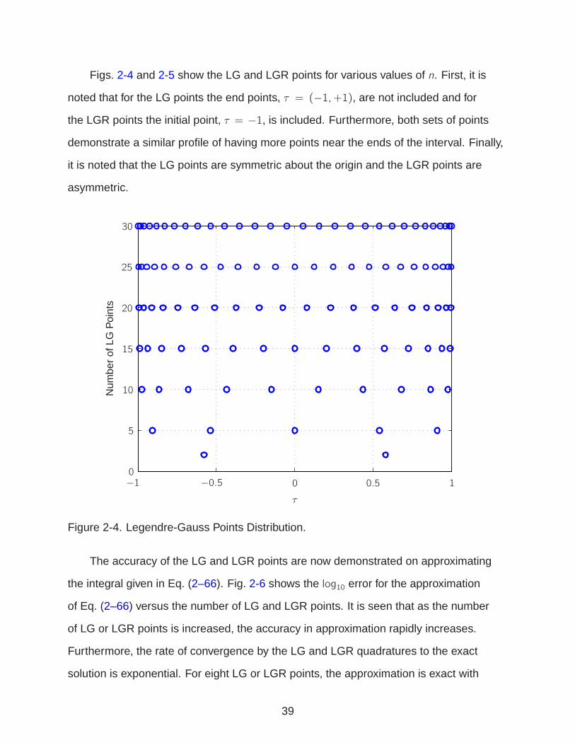
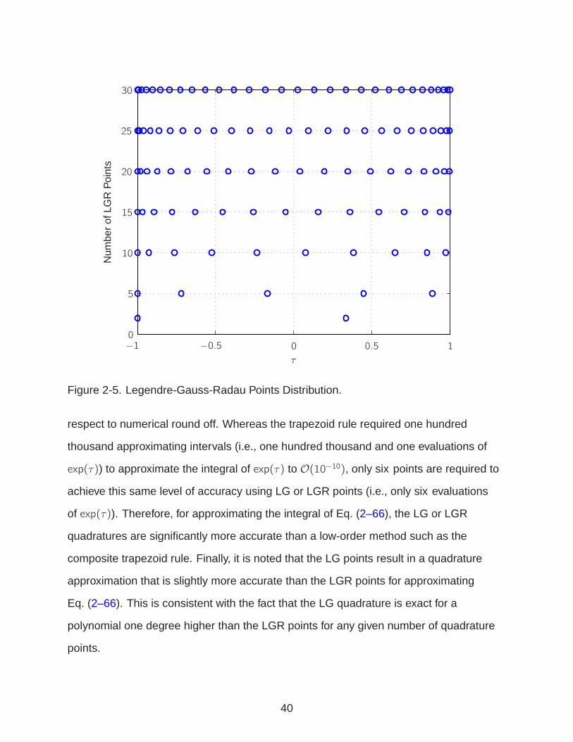
Figs. 2-4 and 2-5 show the LG and LGR points for various values of n. First, it is
noted that for the LG points the end points, τ = (−1,+1), are not included and for
the LGR points the initial point, τ = −1, is included. Furthermore, both sets of points
demonstrate a similar profile of having more points near the ends of the interval. Finally,
it is noted that the LG points are symmetric about the origin and the LGR points are
asymmetric.
00−1 −0.5 0.5 1
5
10
τ
Num
ber
ofLG
Poi
nts
15
20
25
30
Figure 2-4. Legendre-Gauss Points Distribution.
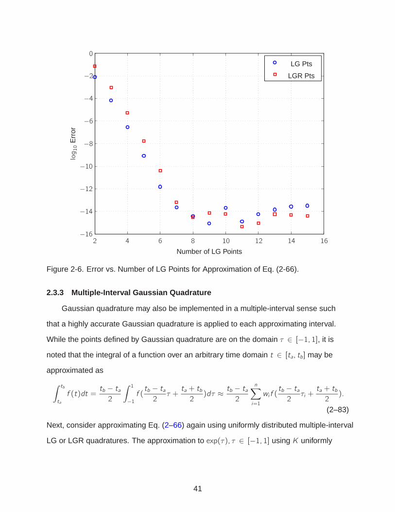
The accuracy of the LG and LGR points are now demonstrated on approximating
the integral given in Eq. (2–66). Fig. 2-6 shows the log10 error for the approximation
of Eq. (2–66) versus the number of LG and LGR points. It is seen that as the number
of LG or LGR points is increased, the accuracy in approximation rapidly increases.
Furthermore, the rate of convergence by the LG and LGR quadratures to the exact
solution is exponential. For eight LG or LGR points, the approximation is exact with
39
00−1 −0.5 0.5 1
5
10
15
20
25
30
τ
Num
ber
ofLG
RP
oint
s
f
Figure 2-5. Legendre-Gauss-Radau Points Distribution.
respect to numerical round off. Whereas the trapezoid rule required one hundred
thousand approximating intervals (i.e., one hundred thousand and one evaluations of
exp(τ)) to approximate the integral of exp(τ) to O(10−10), only six points are required to
achieve this same level of accuracy using LG or LGR points (i.e., only six evaluations
of exp(τ)). Therefore, for approximating the integral of Eq. (2–66), the LG or LGR
quadratures are significantly more accurate than a low-order method such as the
composite trapezoid rule. Finally, it is noted that the LG points result in a quadrature
approximation that is slightly more accurate than the LGR points for approximating
Eq. (2–66). This is consistent with the fact that the LG quadrature is exact for a
polynomial one degree higher than the LGR points for any given number of quadrature
points.
40
0
2 4
−2
−4
−6
−8
−10
−12
−14
−166 8 10 12 14 16
Number of LG Points
log10
Err
orLG Pts
LGR Pts
Figure 2-6. Error vs. Number of LG Points for Approximation of Eq. (2-66).
2.3.3 Multiple-Interval Gaussian Quadrature
Gaussian quadrature may also be implemented in a multiple-interval sense such
that a highly accurate Gaussian quadrature is applied to each approximating interval.
While the points defined by Gaussian quadrature are on the domain τ ∈ [−1, 1], it is
noted that the integral of a function over an arbitrary time domain t ∈ [ta, tb] may be
approximated as
∫ tb
ta
f (t)dt =tb − ta2
∫ 1
−1
f (tb − ta2
τ +ta + tb2)dτ ≈ tb − ta
2
n∑
i=1
wi f (tb − ta2
τi +ta + tb2).
(2–83)
Next, consider approximating Eq. (2–66) again using uniformly distributed multiple-interval
LG or LGR quadratures. The approximation to exp(τ), τ ∈ [−1, 1] using K uniformly
41
distributed intervals is
∫ +1
−1
exp(τ)dτ ≈K∑
k=1
tk − tk−12
n∑
i=1
wi f (tk − tk−12
τi +tk + tk−12
) (2–84)
where tk−1 and tk define the beginning and end of the k th approximating interval,
respectively, and n are the number of LG or LGR quadrature points in each interval.
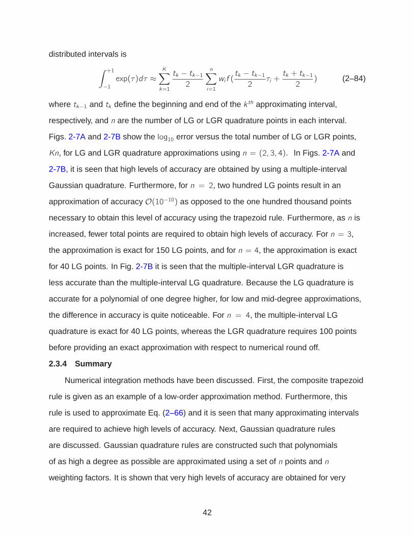
Figs. 2-7A and 2-7B show the log10 error versus the total number of LG or LGR points,
Kn, for LG and LGR quadrature approximations using n = (2, 3, 4). In Figs. 2-7A and
2-7B, it is seen that high levels of accuracy are obtained by using a multiple-interval
Gaussian quadrature. Furthermore, for n = 2, two hundred LG points result in an
approximation of accuracy O(10−10) as opposed to the one hundred thousand points
necessary to obtain this level of accuracy using the trapezoid rule. Furthermore, as n is
increased, fewer total points are required to obtain high levels of accuracy. For n = 3,
the approximation is exact for 150 LG points, and for n = 4, the approximation is exact
for 40 LG points. In Fig. 2-7B it is seen that the multiple-interval LGR quadrature is
less accurate than the multiple-interval LG quadrature. Because the LG quadrature is
accurate for a polynomial of one degree higher, for low and mid-degree approximations,
the difference in accuracy is quite noticeable. For n = 4, the multiple-interval LG
quadrature is exact for 40 LG points, whereas the LGR quadrature requires 100 points
before providing an exact approximation with respect to numerical round off.
2.3.4 Summary
Numerical integration methods have been discussed. First, the composite trapezoid
rule is given as an example of a low-order approximation method. Furthermore, this
rule is used to approximate Eq. (2–66) and it is seen that many approximating intervals
are required to achieve high levels of accuracy. Next, Gaussian quadrature rules
are discussed. Gaussian quadrature rules are constructed such that polynomials
of as high a degree as possible are approximated using a set of n points and n
weighting factors. It is shown that very high levels of accuracy are obtained for very
42

0
0
−10
10050 150 200
−5
−15
Number of Multi-Interval LG Points
log10
Err
or
n = 2
n = 3
n = 4
A LG Points.
0
0
−10
10050 150 200
−5
−15
Maxim
n = 2
n = 3
n = 4
Number of Multi-Interval LGR Points
log10
Err
or
B LGR Points.
Figure 2-7. Error vs. Number of Multiple-Interval LG or LGR Points for Approximation ofEq. (2–66).
43

few points by using LG or LGR points to approximate the integral of Eq. (2–66).
Finally, multiple-interval Gaussian quadrature are discussed. High levels of accuracy
in quadrature approximation are obtained again for this case for a few number of
approximating points when compared with the composite trapezoid rule. Furthermore,
the LG quadrature is more accurate than the LGR quadrature. It is noted that while
more points are required to accurately approximate Eq. (2–66) using a multiple-interval
Gaussian quadrature than a single interval, a thorough motivation is given as to why a
multiple-interval Gaussian quadrature is desired in constructing the hp–pseudospectral
method of this research in Chapter 3 and Chapter 4.
2.4 Lagrange Polynomial Approximation
The next important concept used in constructing the discretized finite-dimensional
optimization problem of this research is polynomial interpolation. In this research,
Lagrange polynomials are used as a continuous-time approximation to the state
equations of the continuous-time optimal control problem. In a Lagrange polynomial
approximation, a set of n support points, (t1, ... , tn), are used and a polynomial of
degree n− 1 is fitted to these points. A Lagrange polynomial approximation to a function,
f (t), is given by
f (t) =
n∑
j=1
fjLj(t), Lj(t) =
n∏
l=1l 6=j
t − tltj − tl
, (2–85)
where fj = f (tj). It is noted that at the support points tj for j = (1, ... , n), fi = fi .
2.4.1 Single-Interval Lagrange Polynomial Approximations
It is well known that Runge phenomenon exists for Lagrange polynomials for an
arbitrary set of support points. Runge phenomenon is the occurrence of oscillations in
the approximating function, f , between support points. As the number of support points
grows, the magnitude of the oscillations between support points also grows. Runge
phenomenon can be demonstrated on the function
f (τ) =1
1 + 25τ 2, τ ∈ [−1,+1]. (2–86)
44
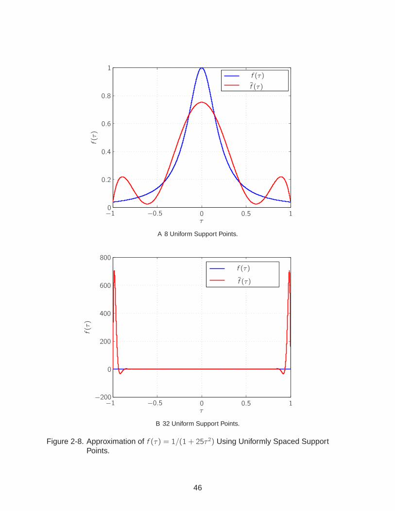
Fig. 2-8 shows the Lagrange polynomial approximation to this function utilizing n =
(8, 32) uniformly distributed support points. It is seen that as the number of points are
increased, the approximation near the ends of the interval become increasingly worse.
Next, consider a Lagrange polynomial approximation to the same function utilizing
n = (8, 32) LG support points. This approximation is shown in Fig. 2-9 and it is seen
that by using LG support points, Runge phenomenon is avoided, and the approximations
become better as the number of support points are increased. Insight into the behavior
of the Lagrange polynomial approximations is exemplified by the following theorem [62].
Theorem: Let t0, t1, ... , tn be distinct real numbers, and let f be a given real valued
function with n + 1 continuous derivatives on the interval It = H(t, t0, t1, ... , tn), with t
some given real number. Then there exists ζ ∈ It such that
f (t)− f (t) = (t − t0) · · · (t − tn)(n + 1)!
f n+1(ζ). (2–87)
Eq. (2–87) defines a limit on the error between the function being approximated and a
Lagrange polynomial approximation of the function. It should be noted at any support
point, the error is zero. In designing an n point Lagrange polynomial approximation,
the only design freedom is in placement of the support points, i.e., changing the
behavior of the numerator term in Eq. (2–87). For uniformly distributed points, the
numerator term becomes excessively large at the ends of the intervals. This results
in the Runge phenomenon that is seen in Fig. 2-8. Furthermore, points defined by
Gaussian quadrature have a structure that they are more densely placed near the ends
of the interval (see again Figs. 2-4 and 2-5). This distribution reduces the magnitude
of the numerator term in Eq. (2–87) at the ends of the intervals, therefore, reducing
the effects of Runge phenomenon. Fig. 2-11 shows the log10 maximum error as a
function of degree of approximating Lagrange polynomial for uniformly distributed
support points and support points defined by LG and LGR points for approximating
Eq. (2–86). It is seen that as the degree of polynomial increases, the Lagrange
45
00−1 −0.5 0.5
1
1
0.2
0.4
0.6
0.8
f (τ)
f (τ)f(τ)
τ
A 8 Uniform Support Points.
0
0−1 −0.5 0.5 1
200
400
600
800
−200
Maxim
f (τ)
f (τ)
f(τ)
τ
B 32 Uniform Support Points.
Figure 2-8. Approximation of f (τ) = 1/(1 + 25τ 2) Using Uniformly Spaced SupportPoints.
46

1.2
−0.2
0
0−1 −0.5 0.5
1
1
0.2
0.4
0.6
0.8
f (τ)
f(τ)
τ
f (τ)
A 8 LG Support Points.
00−1 −0.5 0.5
1
1
0.2
0.4
0.6
0.8
Each
f (τ)
f(τ)
τ
f (τ)
B 32 LG Support Points.
Figure 2-9. Approximation of f (τ) = 1/(1 + 25τ 2) Using LG Support Points.
47

polynomial approximation using a uniformly distributed set of support points diverges.
For a 100th degree polynomial defined with uniformly distributed support points, errors
are O(1030). For a Lagrange polynomial defined by either LG or LGR support points, the
approximation converges to the function in Eq. (2–86). For a 100th degree polynomial,
the errors in approximating this function are O(10−10). Furthermore, unlike the case
of using LG and LGR points for the approximation to integrals, it is noted that when
used as the support points to approximate the function in Eq. (2–86) by a Lagrange
polynomial, there is virtually no difference in approximation error by LG or LGR points.
2.4.2 Multiple-Interval Lagrange Polynomial Approximati ons
Consider approximating Eq. (2–86) using multiple-interval approximations of low
or medium degree. Without using LG or LGR points (or any other set of points that
minimizes Runge phenomenon in a Lagrange polynomial approximation), commonly,
Runge phenomenon is avoided by simply limiting the degree of approximation to be
small. Consider a uniformly distributed set of polynomial approximations such that the
degree of approximation is one, i.e., linear, in each interval. Furthermore, define the
support points for each interval to be the beginning and end of the interval. Fig. 2-11
shows the log10 maximum error in approximating Eq. (2–86) as a function of log10
number of approximating intervals. It is seen that for even one hundred thousand
approximating intervals, errors are still O(10−8).
Next, consider a uniformly distributed multiple-interval approximation utilizing LG
and LGR points as the support points in each interval to approximate Eq. (2–86). It is
noted that the LG and LGR points can be transformed from the time domain τ ∈ [−1, 1]
to an arbitrary time domain t ∈ [ta, tb] by the transformation
t =tb − ta2
τ +ta + tb2. (2–88)
Using n = (4, 6, 8) LG and LGR support points in each interval, Fig. 2-12B shows
the log10 maximum error in approximating Eq. (2–86) versus number of approximating
48
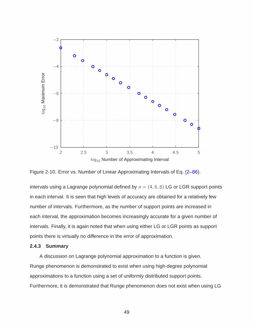
2 2.5 3 4 5
−2
−4
−6
−8
−10
f
3.5 4.5
log10
Max
imum
Err
or
log10 Number of Approximating Interval
Figure 2-10. Error vs. Number of Linear Approximating Intervals of Eq. (2–86).
intervals using a Lagrange polynomial defined by n = (4, 6, 8) LG or LGR support points
in each interval. It is seen that high levels of accuracy are obtained for a relatively few
number of intervals. Furthermore, as the number of support points are increased in
each interval, the approximation becomes increasingly accurate for a given number of
intervals. Finally, it is again noted that when using either LG or LGR points as support
points there is virtually no difference in the error of approximation.
2.4.3 Summary
A discussion on Lagrange polynomial approximation to a function is given.
Runge phenomenon is demonstrated to exist when using high-degree polynomial
approximations to a function using a set of uniformly distributed support points.
Furthermore, it is demonstrated that Runge phenomenon does not exist when using LG
49
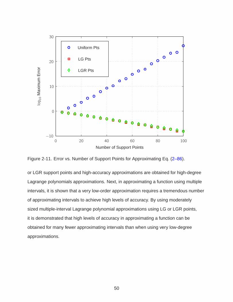
0
0−10
10
40 60 80 100
20
20
30
f
Number of Support Points
log10
Max
imum
Err
or
Uniform Pts
LGR Pts
LG Pts
Figure 2-11. Error vs. Number of Support Points for Approximating Eq. (2–86).
or LGR support points and high-accuracy approximations are obtained for high-degree
Lagrange polynomials approximations. Next, in approximating a function using multiple
intervals, it is shown that a very low-order approximation requires a tremendous number
of approximating intervals to achieve high levels of accuracy. By using moderately
sized multiple-interval Lagrange polynomial approximations using LG or LGR points,
it is demonstrated that high levels of accuracy in approximating a function can be
obtained for many fewer approximating intervals than when using very low-degree
approximations.
50

0
0
−10
10050 150 200
−5
−15Number of Intervals with n Points In Each Interval
log10
Max
imum
Err
orn = 4
n = 6
n = 8
A LG Points.
0
0
−10
10050 150 200
−5
−15Number of Intervals with n Points In Each Interval
log10
Max
imum
Err
or
n = 4
n = 6
n = 8
B LGR Points.
Figure 2-12. Error vs. Number of LG or LGR Intervals for Approximation of Eq. (2–86).
51
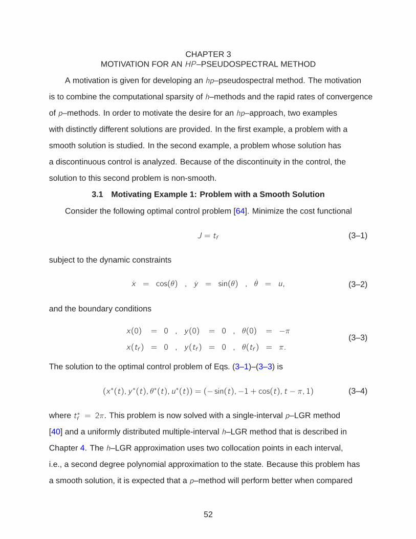
CHAPTER 3MOTIVATION FOR AN HP–PSEUDOSPECTRAL METHOD
A motivation is given for developing an hp–pseudospectral method. The motivation
is to combine the computational sparsity of h–methods and the rapid rates of convergence
of p–methods. In order to motivate the desire for an hp–approach, two examples
with distinctly different solutions are provided. In the first example, a problem with a
smooth solution is studied. In the second example, a problem whose solution has
a discontinuous control is analyzed. Because of the discontinuity in the control, the
solution to this second problem is non-smooth.
3.1 Motivating Example 1: Problem with a Smooth Solution
Consider the following optimal control problem [64]. Minimize the cost functional
J = tf (3–1)
subject to the dynamic constraints
x = cos(θ) , y = sin(θ) , θ = u, (3–2)
and the boundary conditions
x(0) = 0 , y(0) = 0 , θ(0) = −π
x(tf ) = 0 , y(tf ) = 0 , θ(tf ) = π.(3–3)
The solution to the optimal control problem of Eqs. (3–1)–(3–3) is
(x∗(t), y ∗(t), θ∗(t), u∗(t)) = (− sin(t),−1 + cos(t), t − π, 1) (3–4)
where t∗f = 2π. This problem is now solved with a single-interval p–LGR method
[40] and a uniformly distributed multiple-interval h–LGR method that is described in
Chapter 4. The h–LGR approximation uses two collocation points in each interval,
i.e., a second degree polynomial approximation to the state. Because this problem has
a smooth solution, it is expected that a p–method will perform better when compared
52

to an h–method. Fig. 3-1A shows the log10 maximum error at the collocation points
versus the total number of collocation points for the single-interval p–LGR method. It
is seen that for 20 collocation points, the approximation is essentially exact (relative to
roundoff error). Next, Fig 3-1B shows the log10 maximum error at the collocation points
versus the log2 number of approximating intervals for a uniformly distributed h–LGR
approximation. Using the h–LGR method to approximate the solution, the convergence
rates are significantly slower than using a p–method. For an accuracy of O(10−8), the
h–LGR method requires 1024 approximating intervals and 2048 collocation points
while the p–method uses a single approximating interval with only 13 collocation points.
Strictly low-order methods are unable to obtain high levels of accuracy for this problem
in a computationally efficient manner. For this problem, high levels of accuracy in the
approximation are most easily achieved by using a p–method.
3.2 Motivating Example 2: Problem with a Nonsmooth Solution
Consider the following optimal control problem of a soft lunar landing as given in
Ref. [65]. Minimize the cost functional
J =
∫ tf
0
udt (3–5)
subject to the dynamic constraints
h = v , v = −g + u, (3–6)
the boundary conditions
(h(0), v(0), h(tf ), v(tf )) = (h0, v0, hf , vf ) = (10,−2, 0, 0), (3–7)
and the control inequality constraint
umin ≤ u ≤ umax, (3–8)
53
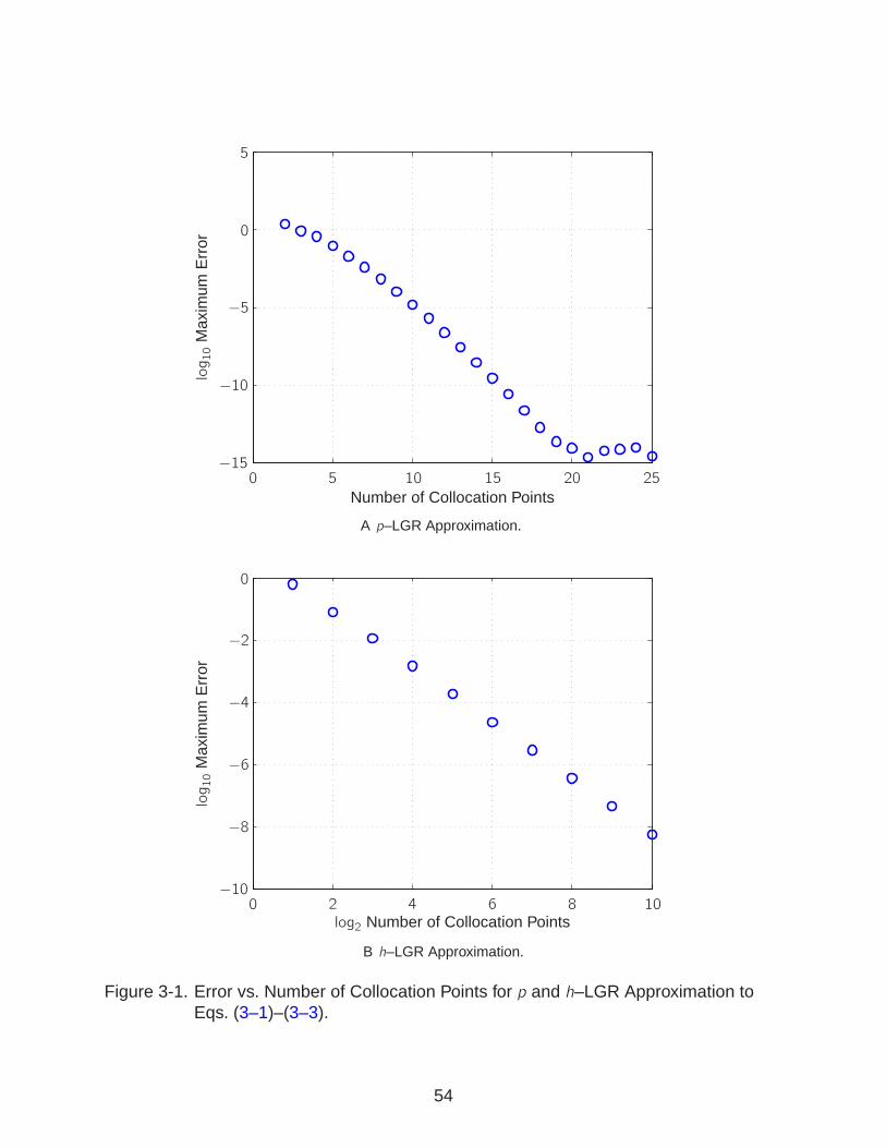
0
0
5
5
−10
10
−5
−1515 20 25
log10
Max
imum
Err
or
Number of Collocation Points
A p–LGR Approximation.
0
0 2 4
−2
−4
−6
−8
−106 8 10
Number of
log10
Max
imum
Err
or
log2 Number of Collocation Points
B h–LGR Approximation.
Figure 3-1. Error vs. Number of Collocation Points for p and h–LGR Approximation toEqs. (3–1)–(3–3).
54

where umin = 0, umax = 3, g = 1.5, tf is free. The optimal solution to this example is
(h∗(t), v ∗(t), u∗(t)) =
(−34t2 + v0t + h0,−32t + v0, 0), t < t∗s
(34t2 + (−3t∗s + v0)t + 3
2t∗s2 + h0,
32t + (−3t∗s + v0), 3), t > t∗s ,
(3–9)
where t∗s is
t∗s =t∗f2+v0
3(3–10)
with
t∗f =2
3v0 +
4
3
√
1
2v 20 +
3
2h0. (3–11)
For the boundary conditions given in Eq. (3–7), t∗s = 1.4154 and t∗f = 4.1641. First,
it is noted in Eq. (3–9) that the control is bang-bang, i.e., the control is at its minimum
value for t ∈ [0, t∗s ] and is at its maximum value for t ∈ [t∗s , t∗f ]. Because of the
discontinuity in the control, the exact solution for the state is non-smooth. Fig. 3-2 shows
the log10 maximum error at the collocation points versus the number of collocation points
for approximating this problem by p and uniformly distributed h–LGR methods. It is
seen that because the solution to the problem is non-smooth, the p–method does not
converge at an exponential rate. Furthermore, the rates of convergence of the p and
h–methods are essentially the same. Therefore, when comparing p and h–methods
with respect to number of collocation points, no significant difference exists between
a p or h–method approximation. The sparsity of the approximating NLPs using p and
h–methods are, however, quite different. A p–method results in a much more dense
NLP as compared to an h–method. Table 3-1 shows the density of the approximating
NLP by p and h–methods for a given number of collocation points. Furthermore, the
CPU time required to solve the given problem is also shown. It is seen in Table 3-1 that
for an equivalent number of collocation points, the p–method results in a problem that
is significantly more computationally expensive because of the density of the NLP. As
the number of collocation points grow for the p–method approximation, the CPU time
55

0
0
−1
1
−2
−410050 150 200
Error
−3
log10
Max
imum
Err
or
Number of Collocation Points
p
h–2
Figure 3-2. Error vs. Collocation Pts for p– and h–LGR Approximation toEqs. (3–5)–(3–8).
required to solve the NLP rapidly grows as well. For the h–method, because of the
sparsity of the NLP, the time required to solve the problem does not grow as rapidly
as with the p–method. Furthermore, it is noted that for 200 collocation points, the
h–method solution time is nearly equivalent to the solution time of the 40 collocation
point p–method. Therefore, if the exponential convergence of a p–method cannot be
guaranteed, a much more computationally efficient NLP is obtained using an h–method
approximation.
3.3 Discussion of Results
The two motivating examples demonstrate a key point in approximating the
solution to general optimal control problems by direct collocation methods: the best
approximation method is problem dependent. Furthermore, in some cases that are
56

Collocation Points p–Matrix Density h–Matrix Density p–CPU Time (s) h–CPU Time (s)20 0.37 0.10 0.07 0.0640 0.35 0.05 0.22 0.1160 0.35 0.037 0.38 0.1280 0.34 0.028 0.54 0.14100 0.34 0.023 0.88 0.16200 0.34 0.012 2.97 0.19
Table 3-1. Matrix Density and CPU Time for p– and h–LGR Methods for Example 2.
simple and smooth, a p–method approximation will provide the best approximating NLP.
In the case of a non-smooth problem without higher order behaviors in the solution, an
h–method approximation will provide the best approximating NLP. In the general case,
a solution to an optimal control problem will have mixed behaviors where some regions
of the trajectory will be smooth, and other regions will be non-smooth. Therefore, a
method that allows for the combination of the strength of either h or p–methods will
be capable of providing highly accurate solutions at a low computational cost. An
hp–pseudospectral method has the flexibility of using the computational sparsity of
low-order h–methods and the high convergence rates of p–methods. The hp–LG and
LGR methods are now described in Chapter 4.
57

CHAPTER 4HP–PSEUDOSPECTRAL METHOD
The hp–LG and LGR pseudospectral methods of this research are now described.
First, the continuous-time optimal control problem of Section 2.1 is reformulated in a
multiple-interval form and the continuous-time first-order necessary conditions are stated
for this multiple-interval formulation. The hp–LG and LGR pseudospectral discretizations
of the multiple-interval optimal control problem are then posed. The KKT conditions
are derived for the hp–LG and LGR methods. Then, the transformed adjoint system for
each method is derived from the KKT conditions and a mapping from the transformed
adjoint system of each method to the continuous-time first-order necessary conditions is
derived. Finally, the sparsity of the NLP defined by the hp–LG and LGR pseudospectral
methods is studied.
4.1 Multiple-Interval Continuous-Time Optimal Control Pro blem Formulation
Consider again the continuous-time optimal control problem of Section 2.1. That is,
minimize the cost functional
J = Φ(x(t0), t0, x(tf ), tf ) +
∫ tf
t0
g(x(t),u(t)) dt, (4–1)
subject to the dynamic constraints
x(t) = f(x(t),u(t)), (4–2)
the inequality path constraints
C(x(t),u(t)) ≤ 0, (4–3)
and the boundary conditions
φ(x(t0), t0, x(tf ), tf ) = 0. (4–4)
Next, consider dividing the problem defined in Eqs. (4–1)–(4–4) into K mesh intervals. A
mesh interval k is defined to begin at the mesh point tk−1 and end at the mesh point tk .
58

Furthermore, let t0 < t1 < t2 < · · · < tK where tK = tf . The time domain in each interval
k , t ∈ [tk−1, tk ], is changed to τ ∈ [−1, 1] by the transformation
τ =2t − (tk−1 + tk)tk − tk−1
. (4–5)
Furthermore, the inverse transformation is given as
t =tk − tk−12
τ +tk−1 + tk2
, (4–6)
and it is noted thatdt
dτ=tk − tk−12
. (4–7)
Next, let each mesh point tk be expressed as a function of the initial time, t0, final time,
tK , and a constant ak , k = (0, ... ,K), as
tk = t0 + ak(tK − t0), (k = 0, ... ,K). (4–8)
It is noted that for t0, a0 = 0 and for tK , aK = 1. Furthermore, because tk−1 < tk ,
ak−1 < ak for k = 1, ... ,K . By expressing each mesh point as a function of t0 and tK ,
the number of free variables corresponding to time is reduced from K + 1 free variables
corresponding to each mesh point to two free variables corresponding to the initial and
final times. This is important for constructing a concise set of necessary conditions for
the optimal control problem and for reducing the number of variables in the discretized
NLP. Let x(k)(τ) and u(k)(τ) be the state and control in the k th mesh interval. Finally,
it is noted that the continuity in the state is enforced at the interior mesh points and
therefore, x(k)(+1) = x(k+1)(−1), (k = 1, ... ,K − 1).
The continuous-time optimal control problem defined by Eqs. (4–1)–(4–4)
expressed as a K interval problem is then to minimize the cost
J = Φ(x(1)(−1), t0, x(K)(+1), tK) +K∑
k=1
tk − tk−12
∫ +1
−1
g(x(k)(τ),u(k)(τ)) dτ , (4–9)
59

subject to the dynamic constraints
dx(k)(τ)
dτ=tk − tk−12
f(x(k)(τ),u(k)(τ)), (k = 1, ... ,K) (4–10)
the inequality path constraints
tk − tk−12
C(x(k)(τ),u(k)(τ)) ≤ 0, (k = 1, ... ,K) (4–11)
the boundary conditions
φ(x(1)(−1), t0, x(K)(+1), tK) = 0, (4–12)
and the interior point constraints
x(k)(+1)− x(k+1)(−1) = 0, (k = 1, ... ,K − 1). (4–13)
It is noted thattk − tk−12
(4–14)
is added to Eq. (4–11) without affecting the constraint such that the optimality conditions
can be posed in a succinct manner.
The first-order optimality conditions of the multiple-interval continuous-time optimal
control problem of Eqs. (4–9)–(4–13) are now stated. Define the augmented Hamiltonian
in each interval k as
H(k)(x(k),λ(k),u(k),γ(k)) = g(k) + 〈λ(k), f(k)〉 − 〈γ(k),C(k)〉. (4–15)
where 〈·, ·〉 is used to denote the standard inner product between two vectors. Using this
definition of the augmented Hamiltonian in each interval, the continuous-time first-order
60
optimality conditions of the problem defined by Eqs. (4–9)–(4–13) are
dx(k)
dτ=tk − tk−12
∇λ(k)H(k), (k = 1, ... ,K), (4–16)
dλ(k)
dτ= −tk − tk−1
2∇x(k)H(k), (k = 1, ... ,K), (4–17)
0 = ∇u(k)H(k), (k = 1, ... ,K), (4–18)
λ(1)(−1) = −∇x(1)(−1) (Φ− 〈ψ,φ〉) , (4–19)
λ(k)(1) = λ(k+1)(−1) + ρ(k), (k = 1, ... ,K − 1) (4–20)
λ(K)(+1) = ∇x(K)(+1) (Φ− 〈ψ,φ〉) , (4–21)
0 =
K∑
i=1
ak−1 − ak2
∫ 1
−1
H(k)dτ +∇t0 (Φ− 〈ψ,φ〉) , (4–22)
0 =
K∑
i=1
ak − ak−12
∫ 1
−1
H(k)dτ +∇tf (Φ− 〈ψ,φ〉) . (4–23)
where ρ(k) is the difference in λ(k)(1) and λ(k+1)(−1) if the costate is discontinuous at a
mesh point k [2].
4.2 hp-Legendre-Gauss Transcription
The hp–LG pseudospectral method is now described. The hp–LG pseudospectral
method is constructed by discretizing the multiple-interval continuous-time optimal
control problem described by Eqs. (4–9)–(4–13). First, the state in each interval k of
the continuous-time optimal control problem is approximated by a Lagrange polynomial
using the initial point, τ (k)0 = −1, and the LG points, (τ (k)1 , ... , τ(k)Nk), where Nk is the
number of LG points used in interval k . The state approximation is then given as
x(k)(τ) ≈ X(k)(τ) =Nk∑
j=0
X(k)j L
(k)j (τ), (4–24)
where X(k)j = X(k)(τ (k)j ). Furthermore, it is noted that in this Chapter, all vector functions
of time are row vectors, i.e., X(k)(τ) = [X (k)1 (τ), ... ,X(k)n (τ)]. Next, an approximation to
the derivative of the state is given by differentiating the approximation of Eq. (4–24) with
61

respect to τ . Therefore, the derivative of the state approximation is given as
dX(k)(τ)
dτ=
Nk∑
j=0
X(k)j L
(k)j (τ). (4–25)
The collocation conditions for interval k are formed by collocating the derivative of the
state approximation with the right hand side of the dynamic constraints of Eq. (4–10) at
the Nk LG points as
Nk∑
j=0
X(k)j D
(k)ij −
(
tk − tk−12
)
f(k)i = 0, (i = 1, ... ,Nk), (4–26)
where f(k)i = f(X(k)i ,U
(k)i ), U(k)i = U(k)(τ (k)i ) is the discretized control approximation, and
D(k)ij = L
(k)j (τ
(k)i ), (i = 1, ... ,Nk , j = 1, ... ,Nk + 1) (4–27)
is the Nk × (Nk + 1) Gauss pseudospectral differentiation matrix [22, 26, 35, 36] in the
k th mesh interval. It should be noted that the state approximation is a continuous-time
Lagrange polynomial approximation with Nk + 1 support points while the control is
calculated discretely at the Nk collocation points. The inequality path constraints of
Eq. (4–11) are enforced at the Nk collocation points in each interval k as
tk − tk−12
C(k)(X(k)i ,U
(k)i ) ≤ 0, (i = 1, ... ,Nk). (4–28)
Next, it is noted that thus far the state approximation only uses the initial point, τ0 = −1,
and the Nk LG points in each interval. No discrete approximation as of yet has been
made for the state at the final point in each interval, τ (k)Nk+1 = +1. In order to approximate
the state at the final point in each interval, the following LG quadrature is used
X(k)Nk+1
= X(k)0 +
tk − tk−12
Nk∑
i=1
w(k)i f
(k)i . (4–29)
62

where w (k)j are the Legendre-Gauss weights in interval k . Next, the state is enforced to
be continuous between mesh intervals, i.e.,
X(k)Nk+1
= X(k+1)0 , (k = 1, ... ,K − 1). (4–30)
In order to increase the computational efficiency of the approximating NLP, a single
variable is used for X(k)Nk+1 and X(k+1)0 for k = (1, ... ,K − 1). Therefore, Eq. (4–29) is then
expressed as
X(k+1)0 = X
(k)0 +
tk − tk−12
Nk∑
i=1
w(k)i f
(k)i , (k = 1, ... ,K − 1) (4–31)
X(K)NK+1
= X(K)0 +
tK − tK−12
NK∑
i=1
w(K)i f
(K)i
and Eq. (4–30) can be ignored as it is being explicitly taken into account. Finally, the
cost functional of Eq. (4–9) is approximated using a multiple-interval LG quadrature as
J ≈ Φ(X(1)0 , t0,X(K)NK+1, tK) +K∑
k=1
Nk∑
j=1
(
tk − tk−12
)
w(k)j g
(k)j , (4–32)
where g(k)j = g(X(k)j ,U
(k)j ).
The discretized hp–LG pseudospectral approximation to the continuous-time
optimal control problem of Eqs. (4–9)–(4–13) is now stated. The hp–LG pseudospectral
approximation is to minimize the cost
J = Φ(X(1)0 , t0,X
(K)NK+1, tK) +
K∑
k=1
Nk∑
j=1
(
tk − tk−12
)
w(k)j g
(k)j , (4–33)
subject to the collocation conditions
Nk∑
j=0
X(k)j D
(k)ij −
(
tk − tk−12
)
f(k)i = 0, (i = 1, ... ,Nk , k = 1, ... ,K − 1), (4–34)
the inequality path constraints
tk − tk−12
C(k)(X(k)i ,U
(k)i ) ≤ 0, (i = 1, ... ,Nk , k = 1, ... ,K − 1), (4–35)
63
the quadrature constraints
X(k+1)0 = X
(k)0 +
tk − tk−12
Nk∑
i=1
w(k)i f
(k)i , (k = 1, ... ,K − 1) (4–36)
X(K)NK+1
= X(K)0 +
tK − tK−12
NK∑
i=1
w(K)i f
(K)i ,
and the boundary conditions
φ(X(1)0 , t0,X
(K)NK+1, tK) = 0. (4–37)
The problem defined by Eqs. (4–33)–(4–37) is the discrete hp–LG pseudospectral
approximation to the continuous-time optimal control problem defined by Eqs. (4–9)–(4–13).
It is noted that the formulation presented allows for an arbitrary number of intervals, with
arbitrary placement, and with an arbitrary number of LG collocation points in each
interval. That is, the hp–LG method presented has the flexibility of approximating a
continuous-time optimal control problem in any manner desired by using LG points.
A few key properties of the hp–LG pseudospectral method are now stated. First, the
discretization points are defined as the points at which the state is approximated. The
discretization points in an interval k , therefore, are the Nk + 2 points, (τ (k)0 , ... , τ(k)Nk+1).
It is noted that control is approximated at the Nk collocation points, (τ (k)1 , ... , τ(k)Nk).
Next, a well-defined Nthk –degree polynomial approximation to the state is given by
Eq. (4–24). However, no well-defined approximating polynomial is given for the control.
It is interesting to note how the discretization points and collocation points differ for
the hp–LG pseudospectral method. When using a single approximating interval as
shown in Fig. 4-1A, the discretization points differ from the collocation points in that the
discretization points are the collocation points plus the end points. Furthermore, for a
multiple-interval discretization as is seen in Fig. 4-1B, the discretization points differ from
the collocation points in that the discretization points include the collocation points and
64

7
9
03−1 −0.5 0.5 1
4
5
6
8
10
Pol
ynom
ialD
egre
e Collocation Points
Discretization Points
t
A Single-Interval Collocation Points and DiscretizationPoints.
7
02
3
−1 −0.5 0.5 1
4
5
6
8
Collocation Points
Discretization Points
t
Num
ber
ofIn
terv
als
B Multiple-Interval Collocation Points and DiscretizationPoints.
Figure 4-1. Collocation and Discretization Points by LG Methods.
all the mesh points. It is interesting to note that the collocation points do not include any
mesh points for the hp–LG pseudospectral method.
4.2.1 The hp–LG Pseudospectral Transformed Adjoint System
The hp–LG transformed adjoint system is now derived. It is shown that the hp–LG
transformed adjoint system is a discrete representation of the continuous-time first-order
65

necessary conditions of Eqs. (4–16)–(4–23) if the costate of the optimal control problem
is continuous. First, the Lagrangian of the continuous-time optimal control problem
defined by the hp–LG pseudospectral method is given as
L = Φ(X(1)0 ,X
(K)NK+1)− 〈Ψ,φ(X(1)0 ,X(K)NK+1〉 (4–38)
+
K∑
k=1
Nk∑
j=1
(
tk − tk−12
(w(k)j g
(k)j − 〈Γ(k)j ,C
(k)j 〉)
−〈Λ(k)j ,D(k)j ,1:NkX(k)1:Nk+D
(k)j ,0 X
(k)0 − tk − tk−1
2f(k)j 〉
)
−K−1∑
k=1
〈π(k),X(k+1)0 − X(k)0 − tk − tk−12
Nk∑
j=1
w(k)j f
(k)j 〉
−〈π(K),X(K)Nk+1 − X(K)0 − tK − tK−1
2
NK∑
j=1
w(K)j f
(K)j 〉,
where Λ(k), Γ(k), π(k), and Ψ are the multipliers associated with Eqs. (4–34), (4–35),
(4–36), and (4–37). Furthermore, D(k)j ,1:Nk is the j th row and first through Nthk columns
of D(k) and X(k)1:Nk are the first through Nthk rows of X(k). Next, the KKT conditions are
given by differentiating the Lagrangian with respect to X(k)j , j = 1, ... ,NK + 1 and
U(k)j , j = 1, ... ,Nk in each interval k as well as t0 and tK and setting these derivatives
66

equal to zero. The KKT conditions are
0 = ∇U
(
w(k)j g
(k)j + 〈Λ(k)j + w
(k)j π(k), f
(k)j 〉 (4–39)
−〈Γ(k)j ,C(k)j 〉
)
, (k = 1, ... ,K , j = 1, ... ,Nk)
D(k)T
j Λ(k) =tk − tk−12
∇X(
w(k)j g
(k)j + 〈Λ(k)j + w
(k)j π(k), f
(k)j 〉 (4–40)
−〈Γ(k)j ,C(k)j 〉
)
, (k = 1, ... ,K , j = 1, ... ,Nk)
D(1)T
0 Λ(1) − π(1) = ∇
X(1)0(Φ− 〈Ψ,φ〉), (4–41)
D(k)T
0 Λ(k) − π(k) = −π(k−1), (k = 2, ... ,K), (4–42)
π(K) = ∇X(K)NK+1
(Φ− 〈Ψ,φ〉), (4–43)
0 = ∇t0(Φ− 〈Ψ,φ〉) (4–44)
+
K∑
k=1
Nk∑
j=1
(
ak−1 − ak2
(w(k)j g
(k)j + 〈Λ(k)j , f
(k)j 〉 − 〈Γ(k)j ,C
(k)j 〉)
)
K−1∑
k=1
ak−1 − ak2
〈π(k),Nk∑
j=1
w(k)j f
(k)j 〉+ aK−1 − aK
2〈πK ,
NK∑
j=1
w(K)j f
(K)j 〉
(k = 1, ... ,K , j = 1, ... ,Nk)
0 = ∇tf (Φ− < Ψ,φ >) (4–45)
+
K∑
k=1
Nk∑
j=1
(
ak − ak−12
(w(k)j g
(k)j + 〈Λ(k)j , f
(k)j 〉 − 〈Γ(k)j ,C
(k)j 〉)
)
+
K−1∑
k=1
ak − ak−12
〈π(k),Nk∑
j=1
w(k)j f
(k)j 〉+ aK − aK−1
2〈πK ,
NK∑
j=1
w(K)j f
(K)j 〉
(k = 1, ... ,K , j = 1, ... ,Nk)
where DT
j is the j th row of DT. In comparing Eq. (4–41) with Eq. (4–19), the costate
approximation at t = t0 is given as
λ(1)0 = −D(1)T0 Λ(1) + π(1) (4–46)
Next, in comparing Eq. (4–43) with Eq. (4–21), the costate approximation at t = tf is
given as
λ(K)NK+1
= π(K). (4–47)
67

Consider the change of variables
ψ = Ψ, (4–48)
γ(k)j =
Γ(k)j
w(k)j
, (k = 1, ... ,K , j = 1, ... ,Nk) (4–49)
λ(k)j =
Λ(k)
w(k)j
+ π(k), (k = 1, ... ,K , j = 1, ... ,Nk), (4–50)
and define the matrix D(k)† [40] as
D(k)†ij = −
w(k)j
w(k)i
D(k)ji , (k = 1, ... ,K , j = 1, ... ,Nk) (4–51)
D(k)†i ,Nk+1
= −Nk∑
j=1
D(k)†ij , (i = 1, ... ,Nk). (4–52)
D(k)† defines the differentiation matrix associated with a Lagrange polynomial using the
LG points, (τ (k)1 , ... , τ(k)Nk) and the final point τ (k)Nk+1 in an interval k [40]. Substituting the
change of variables given in Eqs. (4–46)–(4–52) into (4–39)–(4–43), the LG transformed
68

adjoint system is given as
(D(k)†j ,1:Nk
λ(k) +D(k)†j ,Nk+1
π(k)) = −tk − tk−12
∇XH(X(k)j ,U(k)j ,γ
(k)j ,λ
(k)j ), (4–53)
(k = 1, ... ,K , j = 1, ... ,Nk)
0 = ∇UH(X(k)j ,U
(k)j ,γ
(k)j ,λ
(k)j ), (4–54)
(k = 1, ... ,K , j = 1, ... ,Nk)
λ(1)0 = −∇
X(1)0(Φ− 〈ψ,φ〉), (4–55)
λ(K)NK+1
= ∇X(K)NK+1
(Φ− 〈ψ,φ〉), (4–56)
π(k) − π(k−1) = −tk − tk−12
Nk∑
j=1
w(k)j ∇XH(X(k)j ,U
(k)j ,γ
(k)j ,λ
(k)j ),(4–57)
(k = 2, ... ,K),
0 =
K∑
k=1
ak−1 − ak2
Nk∑
j=1
w(k)j H(X
(k)j ,U
(k)j ,γ
(k)j ,λ
(k)j ) (4–58)
+∇t0(Φ− 〈γ,ψ〉),
0 =
K∑
k=1
ak − ak−12
Nk∑
j=1
w(k)j H(X
(k)j ,U
(k)j ,γ
(k)j ,λ
(k)j ) (4–59)
+∇tf (Φ− 〈γ,ψ〉),
where it is noted that Eq. (4–57) is formed by comparing Eqs. (4–40) and (4–42) and the
identity [40]
D(k)i ,0 = −
Nk∑
j=1
D(k)ij , (i = 1, ... ,Nk). (4–60)
From Eq. (4–57), noting that λ(K)NK+1 = π(K) ,
λ(K)0 = π(K−1). (4–61)
Suppose the costate is continuous at mesh point K − 1. This then implies λ(K)0 = λ(K−1)Nk+1
and using Eq. (4–57) again, we obtain
λ(K−1)0 = π(K−2). (4–62)
69
Next, suppose the costate is continuous at all the mesh points k = 1, ... ,K − 1. Then the
costate at the mesh points are given as
λ(k+1)0 = λ
(k)Nk+1
= π(k), (k = 1, ... ,K − 1). (4–63)
In the case where the costate is continuous at every mesh point, the transformed
adjoint system is a discrete representation of the continuous-time first-order necessary
conditions.
Next, suppose that the costate is discontinuous at a mesh point M ∈ [1, ... ,K − 1].
Then
π(M) = λ(M+1)0 = λ
(M)NM+1
− ρ(M) (4–64)
where ρ(M) is the difference between λ(M)NM+1 and λ(M+1)0 . If the costate is discontinuous
at mesh point M, π(M) 6= λ(M)NM+1 in Eq. (4–53). Therefore, Eq. (4–53) is not a discrete
approximation to the continuous-time costate dynamics. As a result, the transformed
adjoint system given in Eqs. (4–53)–(4–59) is not a discrete representation of the
first-order optimality conditions given in Eqs. (4–16)–(4–23).
4.2.2 Sparsity of the hp–LG Pseudospectral Method
The sparsity of the hp–LG pseudospectral method is now described. It is noted that
the only dense blocks of non-zero numbers that occur in the NLP defined by the hp–LG
pseudospectral method are a result of the Lagrange polynomial approximation to the
state in each interval in Eq. (4–34) and also the quadrature constraints of Eq. (4–36).
The size of these dense blocks are dependent upon the degree of approximating
polynomial, Nk , in each interval. The constraint Jacobian for the hp–LG pseudospectral
method is now described in detail. First, define the total number of collocation points as
N =
K∑
i=1
Ni . (4–65)
Next, the total vector of NLP variables corresponding to the discretized state, control,
and initial and final time is constructed. Define the (N + K + 1)n × 1 vector zx as the
70
vector containing each component of the state at all the discretization points, i.e.,
zx =
χ1...
χn
(4–66)
where χi is the (N + K + 1) × 1 vector corresponding to the i th component of the state
evaluated at the discretization points. Furthermore, define the Nm × 1 vector zu as the
vector containing each component of the control evaluated at the collocation points, i.e.,
zu =
σ1
...
σm
(4–67)
where σi is the N × 1 vector corresponding to the i th component of the control at all of
the collocation points. Therefore, the total vector of NLP variables is
z =
zx
zu
t0
tf
(4–68)
and the total number of NLP variables is (N + K + 1)n + Nm + 2.
Next, the total vector of NLP constraints are constructed. Define the Nn × 1 vector
yD as the vector containing the collocation conditions for each component of the state,
i.e.,
yD =
ζ1...
ζn
(4–69)
where ζ i is the N × 1 vector corresponding to the collocation conditions for the i th
component of the state. Next, define the Ns × 1 vector yC as the vector containing the
71

inequality path constraints:
yC =
η1...
ηs
(4–70)
where ηi is the N×1 vector corresponding to the i th inequality path constraint. Define the
Kn × 1 vector yQ to be the vector of quadrature constraints in Eq. (4–36). Finally, define
the q × 1 vector yE to be the vector of boundary conditions in Eq. (4–37). Therefore, the
total vector of constraints for the hp–LG method is
y =
yD
yC
yQ
yE
(4–71)
and the total number of NLP constraints is Nn + Ns + Kn + q. It is interesting to note
for the hp–LG pseudospectral method, the size of the NLP problem (i.e., the number
of variables and constraints) are dependent upon the number of collocation points, N,
and the number of approximating intervals, K . As the number of collocation points or
number of approximating intervals grows large for the hp–LG pseudospectral method, so
do the number of variables and constraints in the NLP. Finally, the constraint Jacobian
for the hp–LG pseudospectral method is given as
G(z) =∂y
∂z. (4–72)
The density of the constraint Jacobian is now examined. For the constraints
associated with yC , each row corresponds to an inequality path constraint evaluated
at a collocation point. By inspection of Eq. (4–35), it is seen that at each collocation
point, the inequality path constraints are only a function of the state and control at that
collocation point and the initial and final time. Therefore, the rows of yC are sparse (i.e., ,
only n + m + 2 elements in any row are non-zero; the remaining (N + K)n + (N − 1)m
72

elements are zero). Furthermore, yE is only a function of the state at the initial and final
time and the initial and final time. Therefore, the rows of yE are sparse as well.
yD and yQ introduce the density of the hp–LG pseudospectral method. It is seen in
Eq. (4–34) that the collocation condition for any component of the state evaluated at any
collocation point is a function of the state and control at that collocation point, the initial
and final time, and Nk additional variables corresponding to the Lagrange polynomial
approximation to the state. Therefore, as Nk grows large in any approximating interval,
the number of non-zero elements in any row of yD grows large as well. Finally, it is
seen in Eq. (4–36) that for each quadrature constraint, the constraint is a function of
Nkn variables corresponding to the state, Nkm variables corresponding to the control,
the initial and final time, and two additional variables corresponding to the initial state
and final state in interval k . Therefore, again, as Nk grows large in any approximating
intervals, so does the number of non-zero entries in any row of yQ .
Figs. 4-2 and 4-3 shows a qualitative representation of the constraint Jacobian
for the hp–LG pseudospectral method. Fig. 4-2 represents an hp–LG pseudospectral
approximation where Nk is large in each approximating interval and Fig.4-3 represents
an hp–LG pseudospectral approximation where Nk is small in each approximating
interval. It is seen that for large Nk , large, dense blocks arise in the constraint Jacobian
corresponding to the rows of yD and yQ . For small values of Nk , the dense blocks are
much smaller. Therefore, the sparsity of an hp–LG pseudospectral method is dependent
upon Nk , or, the degree of polynomial approximation within any interval. Low-degree
approximations result in a sparse NLP while high-degree approximations result in a
dense NLP.
4.3 hp–Legendre-Gauss-Radau Transcription
The hp–LGR pseudospectral method is now described. The hp–LGR pseudospectral
method is constructed by discretizing the continuous-time optimal control problem
described by Eqs. (4–9)–(4–13). First, the state in each interval k of the continuous-time
73
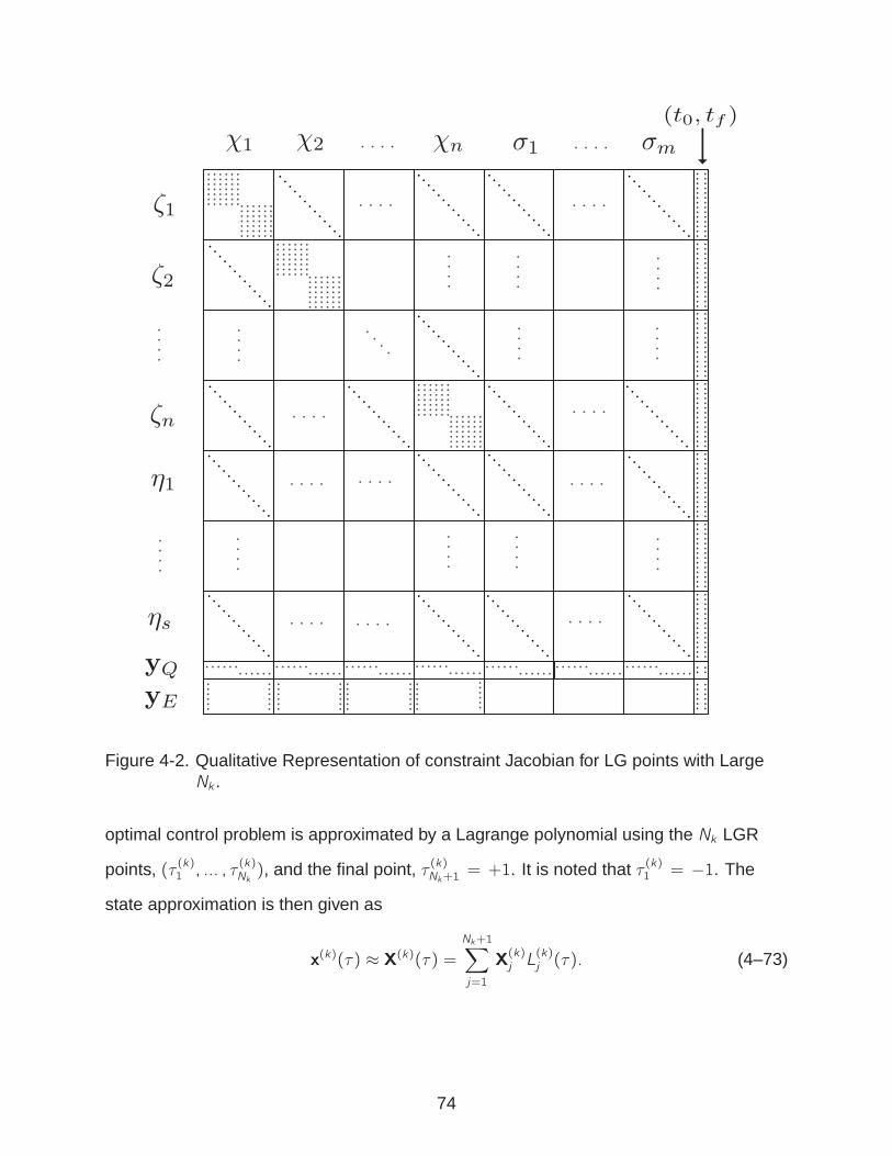
Figure 4-2. Qualitative Representation of constraint Jacobian for LG points with LargeNk .
optimal control problem is approximated by a Lagrange polynomial using the Nk LGR
points, (τ (k)1 , ... , τ(k)Nk), and the final point, τ (k)Nk+1 = +1. It is noted that τ (k)1 = −1. The
state approximation is then given as
x(k)(τ) ≈ X(k)(τ) =Nk+1∑
j=1
X(k)j L
(k)j (τ). (4–73)
74
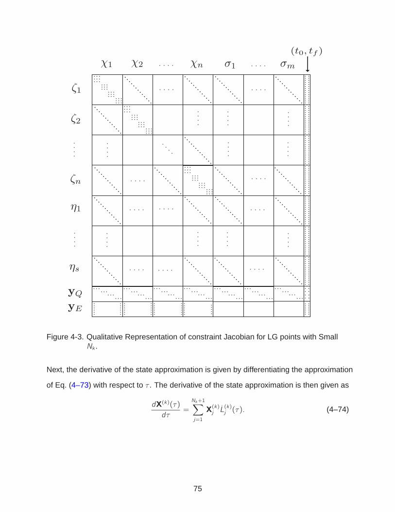
Figure 4-3. Qualitative Representation of constraint Jacobian for LG points with SmallNk .
Next, the derivative of the state approximation is given by differentiating the approximation
of Eq. (4–73) with respect to τ . The derivative of the state approximation is then given as
dX(k)(τ)
dτ=
Nk+1∑
j=1
X(k)j L
(k)j (τ). (4–74)
75

The collocation conditions are then enforced at the Nk LGR points as
Nk+1∑
j=1
X(k)j D
(k)ij − tk − tk−1
2f(k)i = 0, (i = 1, ... ,Nk , k = 1, ... ,K), (4–75)
where
D(k)ij = L
(k)j (τ
(k)i ), (i = 1, ... ,Nk , j = 1, ... ,Nk + 1), (4–76)
is the Nk × (Nk + 1) Radau pseudospectral differentiation matrix [39] in the k th mesh
interval. The inequality path constraints of Eq. (4–11) are enforced at the Nk collocation
points in each interval k as
tk − tk−12
C(k)(X(k)i ,U
(k)i ) ≤ 0, (i = 1, ... ,Nk , k = 1, ... ,K). (4–77)
Next, the state is enforced to be continuous between mesh intervals, i.e.,
X(k)Nk+1
= X(k+1)1 . (4–78)
In order to increase the computational efficiency of the approximating NLP, a single
variable is used for X(k)Nk+1 and X(k+1)1 for k = (1, ... ,K − 1). Therefore, Eq. (4–75) is then
written as
D(k)j ,1:NkX(k)1:Nk+D
(k)j ,Nk+1
X(k+1)1 − tk − tk−1
2f(k)j = 0 (k = 1, ... ,K − 1), (4–79)
D(K)j ,1:NK
X(K)1:NK+D
(K)j ,NK+1
X(K)NK+1
− tK − tK−12
f(K)j = 0
and Eq. (4–78) can be ignored as it is being explicitly taken into account. Finally,
the cost functional of Eq. (4–9) is then approximated using a multiple-interval LGR
quadrature as
J ≈ Φ(X(1)1 , t0,X(K)NK+1, tK) +K∑
k=1
Nk∑
j=1
(
tk − tk−12
)
w(k)j g
(k)j , (4–80)
where w (k)j are the Legendre-Gauss-Radau weights [63] in interval k .
76

The discretized hp–LGR pseudospectral approximation to the continuous-time
optimal control problem is now stated. The hp–LGR pseudospectral approximation is to
minimize the cost
J = Φ(X(1)1 , t0,X
(K)NK+1, tK) +
K∑
k=1
Nk∑
j=1
(
tk − tk−12
)
w(k)j g
(k)j , (4–81)
subject to the collocation conditions
D(k)j ,1:NkX(k)1:Nk+D
(k)j ,Nk+1
X(k+1)1 − tk − tk−1
2f(k)j = 0 (k = 1, ... ,K − 1), (4–82)
D(K)j ,1:NK
X(K)1:NK+D
(K)j ,NK+1
X(K)NK+1
− tK − tK−12
f(K)j = 0,
the inequality path constraints
tk − tk−12
C(k)(X(k)i ,U
(k)i ) ≤ 0, (i = 1, ... ,Nk , k = 1, ... ,K). (4–83)
and the boundary conditions
φ(X(1)1 , t0,X
(K)NK+1, tK) = 0. (4–84)
The problem defined by Eqs. (4–81)–(4–84) is the discrete hp–LGR pseudospectral
approximation to the continuous-time optimal control problem defined by Eqs. (4–9)–(4–13).
It is noted that the formulation presented allows for an arbitrary number of intervals, with
arbitrary placement, and an arbitrary number of LGR collocation points in each interval.
Therefore, this method has the flexibility of approximating a continuous-time optimal
control problem in any manner desired by using LGR points.
A few key properties of the hp–LGR pseudospectral method are now stated. First,
the discretization points are defined as the points at which the state is approximated.
The discretization points in an interval k , therefore, are (τ (k)1 , ... , τ(k)Nk+1). It is noted that
the control is approximated at the collocation points, (τ (k)1 , ... , τ(k)Nk). Next, an Nthk degree
polynomial approximation to the state is given by Eq. (4–73). The control on the other
hand, is discretely approximated at the Nk collocation points within each interval. The
77

discretization points and collocation points are now compared for the hp–LGR method.
When using a single approximating interval as is shown in Fig. 4-4A, the discretization
points differ from the collocation points only at the final mesh point, tK . Furthermore,
for a multiple-interval discretization as seen in Fig. 4-4B, again, the discretization
points differ from the collocation points only at the final mesh point. While the hp–LG
pseudospectral method did not approximate the control at any mesh points, the hp–LGR
pseudospectral method approximates the control at every mesh point except the final
mesh point.
4.3.1 The hp-LGR Pseudospectral Transformed Adjoint System
The KKT conditions of the NLP defined by the hp–LGR pseudospectral method are
now derived. The Lagrangian of the hp-LGR pseudospectral method is given as
L = Φ(X(1)1 ,X
(K)NK+1)− 〈Ψ,φ(X(1)1 ,X(K)NK+1〉 (4–85)
+
K∑
k=1
Nk∑
j=1
tk − tk−12
(w(k)j g
(k)j − 〈Γ(k)j ,C
(k)j 〉)
−K−1∑
k=1
Nk∑
j=1
〈Λ(k)j ,D(k)j ,1:NkX(k)1:Nk+D
(k)j ,Nk+1
X(k+1)1 − tk − tk−1
2f(k)j 〉
−NK∑
j=1
〈Λ(K)j ,D(K)j ,1:NK
X(K)1:NK+D
(K)j ,NK+1
X(K)NK+1
− tK − tK−12
f(K)j 〉
where Λ(k), Γ(K), and Ψ are the multipliers associated with Eq. (4–82), Eq. (4–83), and
Eq. (4–84) in mesh interval k , respectively. The KKT conditions of the multiple-interval
Legendre-Gauss-Radau discretization are then given as
D(1)T
j Λ(1) =t1 − t02
∇X(
w(1)j g
(1)j + 〈Λ(1)j , f
(1)j 〉 (4–86)
−〈Γ(1)j ,C(1)j 〉
)
− δ1j
(
−∇X(1)1Φ+∇
X(1)1〈Ψ,φ〉
)
, (j = 1, ... ,N1),
D(k)T
j Λ(k) =tk − tk−12
∇X(
w(k)j g
(k)j + 〈Λ(k)j , f
(k)j 〉 (4–87)
−〈Γ(k)j ,C(k)j 〉
)
− δ1jD(k−1)TNk−1+1
Λ(k−1), (k = 2, ... ,K , j = 1, ... ,Nk).
D(K)T
NK+1Λ(K) = ∇
X(K)NK+1
(Φ− 〈Ψ,φ〉), (4–88)
78
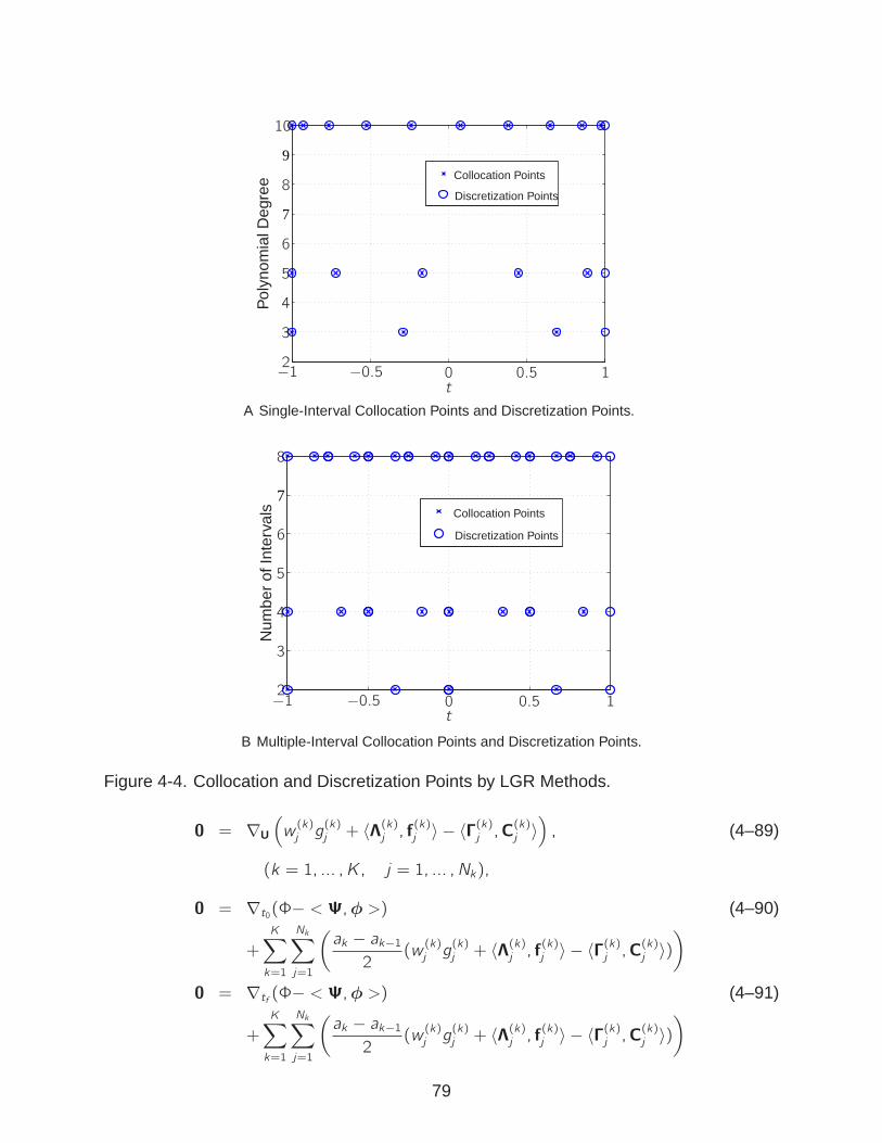
7
9
02
3
−1 −0.5 0.5 1
4
5
6
8
10
Discretization Points
Collocation Points
Pol
ynom
ialD
egre
e
t
A Single-Interval Collocation Points and Discretization Points.
7
02
3
−1 −0.5 0.5 1
4
5
6
8
Discretization Points
Collocation Points
t
Num
ber
ofIn
terv
als
B Multiple-Interval Collocation Points and Discretization Points.
Figure 4-4. Collocation and Discretization Points by LGR Methods.
0 = ∇U
(
w(k)j g
(k)j + 〈Λ(k)j , f
(k)j 〉 − 〈Γ(k)j ,C
(k)j 〉
)
, (4–89)
(k = 1, ... ,K , j = 1, ... ,Nk),
0 = ∇t0(Φ− < Ψ,φ >) (4–90)
+
K∑
k=1
Nk∑
j=1
(
ak − ak−12
(w(k)j g
(k)j + 〈Λ(k)j , f
(k)j 〉 − 〈Γ(k)j ,C
(k)j 〉)
)
0 = ∇tf (Φ− < Ψ,φ >) (4–91)
+
K∑
k=1
Nk∑
j=1
(
ak − ak−12
(w(k)j g
(k)j + 〈Λ(k)j , f
(k)j 〉 − 〈Γ(k)j ,C
(k)j 〉)
)
79

Next, consider the change of variables
ψ = Ψ, (4–92)
γ(k)j =
Γ(k)j
w(k)j
, (k = 1, ... ,K , j = 1, ... ,Nk), (4–93)
λ(k)j =
Λ(k)j
w(k)j
, (k = 1, ... ,K , j = 1, ... ,Nk), (4–94)
π(k) = D(k)TNk+1Λ(k), (k = 1, ... ,K). (4–95)
Furthermore, define the matrix D(k)† [40] as
D(k)†11 = −D(k)11 − 1
w(k)1
, (4–96)
D(k)†ij = −
w(k)j
w(k)i
D(k)ji otherwise. (4–97)
D(k)† is the corresponding differentiation matrix for a Lagrange polynomial approximation
using the Nk LGR points as support points in interval k . Substituting Eqs. (4–92)–(4–97)
into Eqs. (4–86)–(4–91), the transformed adjoint system is given as
D(1)†j λ(1) = −t1 − t0
2∇XH(X(1)j ,U
(1)j ,λ
(1)j ,γ
(1)j ) (4–98)
+δ1j
w(1)1
(−∇X(1)1(Φ− 〈ψ,φ〉)− λ(1)1 ),
D(k)†j λ(k) = −tk − tk−1
2∇XH(X(k)j ,U
(k)j ,λ
(k)j ,γ
(k)j ) (4–99)
+δ1j
w(k)1
(π(k−1) − λ(k)1 ), (k = 2, ... ,K , j = 1, ... ,Nk)
0 = ∇UH(X(k)j ,U
(k)j ,λ
(k)j ,γ
(k)j ), (k = 1, ... ,K , j = 1, ... ,Nk) (4–100)
π(K) = ∇X(K)NK+1
(Φ− 〈ψ,φ〉) (4–101)
0 =
K∑
k=1
ak−1 − ak2
Nk∑
j=1
w(k)j H(X
(1)j ,U
(1)j ,λ
(1)j ,γ
(1)j ) (4–102)
+∇t0(Φ− 〈γ,ψ〉),
0 =
K∑
k=1
ak − ak−12
Nk∑
j=1
w(k)j H(X
(1)j ,U
(1)j ,λ
(1)j ,γ
(1)j ) (4–103)
+∇t0(Φ− 〈γ,ψ〉),
80

where D(k)†j is the j th row of D(k)†. From the results of Ref. [39], we expand Eq. (4–95)
using Eqs. (4–86) and (4–87) to obtain the following relationships:
−∇X(1)1(Φ + 〈ψ,φ〉) = π(1) + t1 − t0
2
N1∑
j=1
w(1)j ∇xH(X(1)j ,U
(1)j ,λ
(1)j ,γ
(1)j ). (4–104)
π(k−1) = π(k) +tk − tk−12
Nk∑
j=1
w(k)j ∇XH(X(k)j ,U
(k)j ,λ
(k)j ,γ
(k)j ). (k = 2, ... ,K) (4–105)
By comparing Eq. (4–21) and Eq. (4–101), the costate approximation at t = tf is given
as
λ(K)NK+1
= π(K). (4–106)
For k = K , the right-hand side of Eq. (4–105) is then an approximation to λ(K)1 .
Therefore,
λ(K)1 = π(K−1). (4–107)
Furthermore, using Eq. (4–107), the final term in Eq. (4–99) disappears for k = K . Next,
let the costate be continuous at mesh point k = K − 1. Then,
λ(K−1)NK−1+1
= λ(K)1 = π(K−1), (4–108)
and for k = K − 1, the right hand side of Eq. (4–105) becomes an approximation to
λ(K−1)1 . Therefore,
λ(K−1)1 = π(K−2), (4–109)
and the final term in Eq. (4–99) disappears for k = K − 1. If the costate is continuous at
every mesh point, then
λ(k)Nk+1
= λ(k+1)1 = π(k), 1 ≤ k ≤ K − 1 (4–110)
and the final term in Eq. (4–99) disappears for k = 2, ... ,K . Furthermore, the left hand
side of Eq. (4–104), then, is an approximation to the costate at t0 and therefore,
λ(1)1 = −∇
X(1)1(Φ + 〈ψ,φ〉) (4–111)
81
and the final term in Eq. (4–98) disappears. Therefore, for the case when the costate
is continuous at every mesh point, the final term in Eqs. (4–98) and (4–99) disappears
and the transformed adjoint system is a discrete representation of the continuous-time
first-order optimality conditions.
Next, suppose that the costate is discontinuous at a particular mesh point M ∈
[1, ... ,K − 1]. Then
π(M) = λ(M+1)1 = λ
(M)NM+1
− ρ(M) (4–112)
where ρ(M) is the difference between λ(M)NM+1 and λ(M+1)1 . Therefore, if the costate
is discontinuous at mesh point M, π(M−1) 6= λ(M)1 in Eq. (4–99). As a result, the
transformed adjoint system given in Eqs. (4–98)–(4–103) is not a discrete representation
of the first-order optimality conditions given in Eqs. (4–16)–(4–23).
4.3.2 Sparsity of the hp–LGR Pseudospectral Method
The sparsity of the hp–LGR pseudospectral method is now described. It is noted
that the only dense blocks of non-zero numbers that occur in the NLP defined by the
hp–LGR pseudospectral method are a result of the Lagrange polynomial approximation
to the state in each interval in Eq. (4–82). The size of these dense blocks are dependent
upon the degree of approximating polynomial, Nk , in each interval. The constraint
Jacobian for the hp–LGR pseudospectral method is now described in detail. The total
vector of NLP variables corresponding to the discretized state, control and initial and
final time is constructed. Define the (N + 1)n × 1 vector zx as the vector containing each
component of the state at all the discretization points, i.e.,
zx =
χ1...
χn
(4–113)
where χn is the (N + 1)× 1 vector corresponding to the i th component of the state at the
discretization points. Furthermore, define the Nm × 1 vector zu as the vector containing
82

each component of the control at all the collocation points, i.e.,
zu =
σ1
...
σm
(4–114)
where σi is the N × 1 vector corresponding to the i th component of the control at the
collocation points. Therefore, the total vector of NLP variables is
z =
zx
zu
t0
tf
(4–115)
and the total number of NLP variables is (N + 1)n + Nm + 2. Next, the total vector of
NLP constraints are constructed. Define the Nn × 1 vector yD as the vector containing
the collocation conditions for each component of the state, i.e.,
yD =
ζ1...
ζn
(4–116)
where ζ i is the N × 1 vector corresponding to the collocation conditions for the i th
component of the state. Next, define the Ns × 1 vector yC as the vector containing the
the inequality path constraints:
yC =
η1...
ηs
(4–117)
where ηi is the N × 1 vector corresponding to the i th inequality path constraint. Finally,
define the q × 1 vector yE to be the vector of boundary conditions in Eq. (4–84).
83
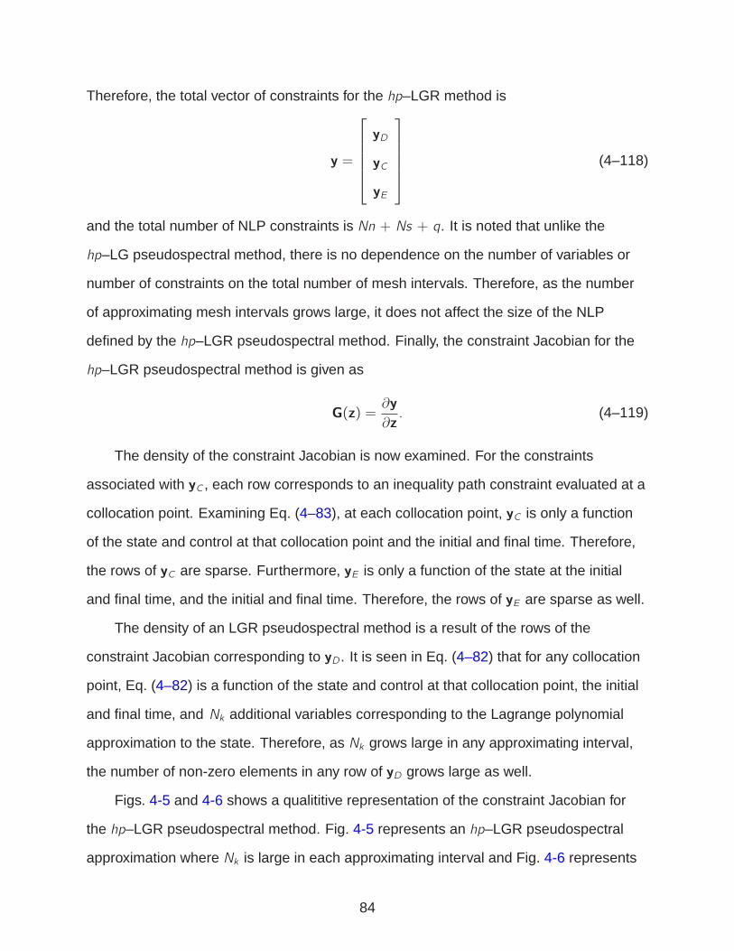
Therefore, the total vector of constraints for the hp–LGR method is
y =
yD
yC
yE
(4–118)
and the total number of NLP constraints is Nn + Ns + q. It is noted that unlike the
hp–LG pseudospectral method, there is no dependence on the number of variables or
number of constraints on the total number of mesh intervals. Therefore, as the number
of approximating mesh intervals grows large, it does not affect the size of the NLP
defined by the hp–LGR pseudospectral method. Finally, the constraint Jacobian for the
hp–LGR pseudospectral method is given as
G(z) =∂y
∂z. (4–119)
The density of the constraint Jacobian is now examined. For the constraints
associated with yC , each row corresponds to an inequality path constraint evaluated at a
collocation point. Examining Eq. (4–83), at each collocation point, yC is only a function
of the state and control at that collocation point and the initial and final time. Therefore,
the rows of yC are sparse. Furthermore, yE is only a function of the state at the initial
and final time, and the initial and final time. Therefore, the rows of yE are sparse as well.
The density of an LGR pseudospectral method is a result of the rows of the
constraint Jacobian corresponding to yD . It is seen in Eq. (4–82) that for any collocation
point, Eq. (4–82) is a function of the state and control at that collocation point, the initial
and final time, and Nk additional variables corresponding to the Lagrange polynomial
approximation to the state. Therefore, as Nk grows large in any approximating interval,
the number of non-zero elements in any row of yD grows large as well.
Figs. 4-5 and 4-6 shows a qualititive representation of the constraint Jacobian for
the hp–LGR pseudospectral method. Fig. 4-5 represents an hp–LGR pseudospectral
approximation where Nk is large in each approximating interval and Fig. 4-6 represents
84
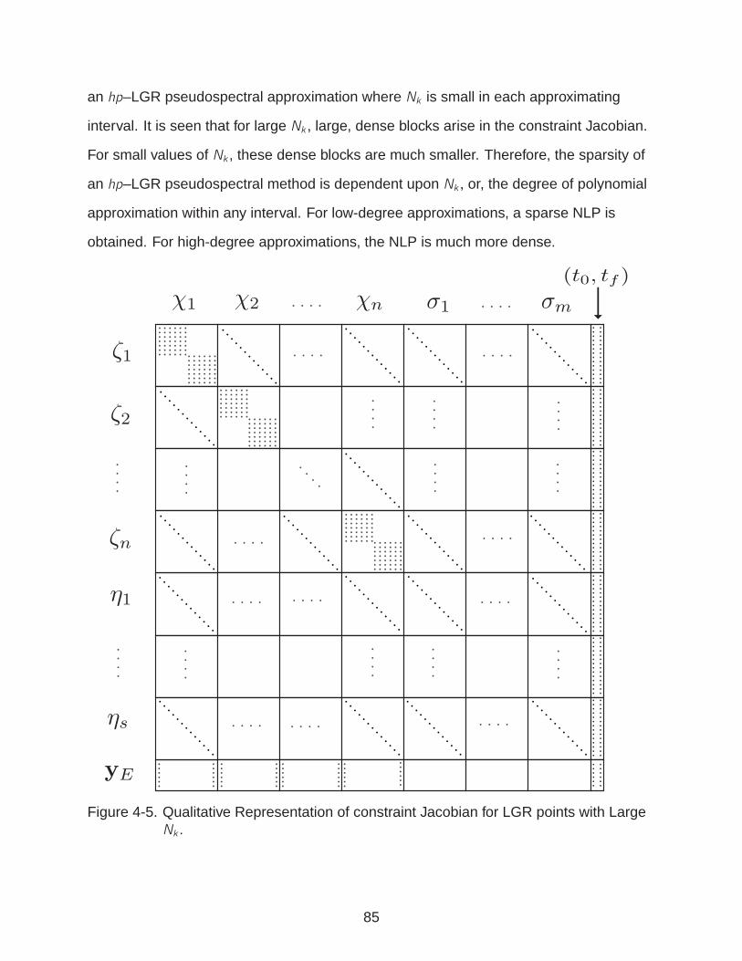
an hp–LGR pseudospectral approximation where Nk is small in each approximating
interval. It is seen that for large Nk , large, dense blocks arise in the constraint Jacobian.
For small values of Nk , these dense blocks are much smaller. Therefore, the sparsity of
an hp–LGR pseudospectral method is dependent upon Nk , or, the degree of polynomial
approximation within any interval. For low-degree approximations, a sparse NLP is
obtained. For high-degree approximations, the NLP is much more dense.
Points
Figure 4-5. Qualitative Representation of constraint Jacobian for LGR points with LargeNk .
85
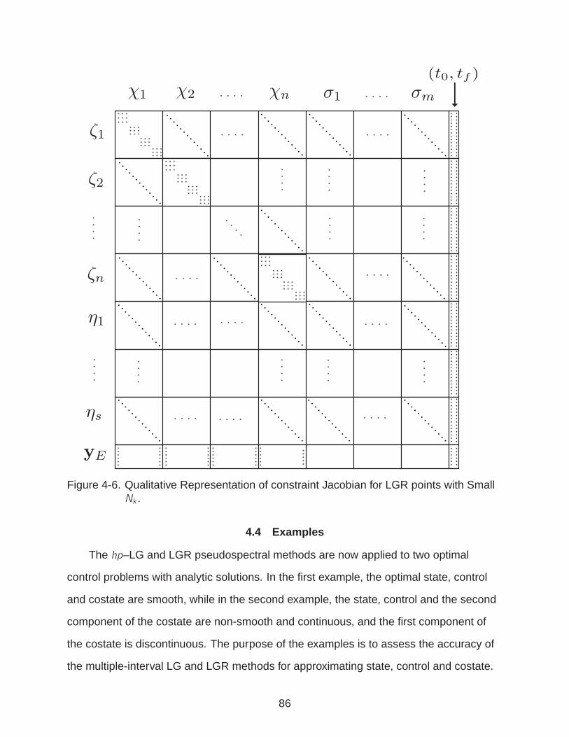
Time
Figure 4-6. Qualitative Representation of constraint Jacobian for LGR points with SmallNk .
4.4 Examples
The hp–LG and LGR pseudospectral methods are now applied to two optimal
control problems with analytic solutions. In the first example, the optimal state, control
and costate are smooth, while in the second example, the state, control and the second
component of the costate are non-smooth and continuous, and the first component of
the costate is discontinuous. The purpose of the examples is to assess the accuracy of
the multiple-interval LG and LGR methods for approximating state, control and costate.
86

The problems are solved by either p or h–methods. For p–method problems, the number
of intervals is fixed and the degree of approximation within each interval is allowed to
vary. For h–method problems, the degree of approximation is fixed within each interval
and the number of intervals is allowed to vary. Finally, the terminology “h–x” denotes an
h–method with x collocation points in every mesh interval.
4.4.1 Example 1 - Problem with a Smooth Solution
Consider the following optimal control problem [39]. Minimize the cost functional
J =1
2
∫ tf
0
(y + u2)dt (4–120)
subject to the dynamic constraint
y = 2y + 2u√y (4–121)
and the boundary conditions
y(0) = 2 (4–122)
y(tf ) = 1 (4–123)
where tf = 5. The exact solution to the optimal control problem is given as
y ∗(t) = x2(t) (4–124)
λ∗y(t) =λx2√y
(4–125)
u∗(t) = −2λ∗(t)√
y ∗(t) (4–126)
where x(t) and λx(t) are given as
x(t)
λx(t)
= exp(At)
x0
λx0
(4–127)
87

where
A =
1 −1
−1 −1
(4–128)
and
x0 =√2 (4–129)
xf = 1 (4–130)
λx0 =xf − B11x0B12
(4–131)
B =
B11 B12
B21 B22
= exp(Atf ). (4–132)
The convergence rates for p and uniformly distributed h–2, h–3, and h–4–LG
and LGR methods are analyzed. Furthermore, the p–method uses only a single
approximating interval. Because the problem has a smooth solution, it is expected that a
p–method will demonstrate the fastest convergence rates for this problem. Furthermore,
because the problem has a continuous costate, it is expected that the multiple-interval
LG and LGR methods will provide accurate approximations to the continuous-time
optimal control problem.
Fig. 4-7 shows the state, costate, and control solution for this problem. As is seen
in Fig. 4-7, the state, costate, and control are all smooth. Figs. 4-8A, 4-8B, and 4-8C
show the maximum state, control, and costate error at the collocation points as a
function of the number of collocation points, respectively, for both the p–LG method
and h–x–LG methods. Furthermore, the maximum state, control, and costate error at
the collocation points as a function of the number of collocation points for p–LGR and
h–x–LGR methods are shown in Figs 4-9A, 4-9B, and 4-9C. Because the solution to
this problem is smooth, for both LG and LGR methods, the p–method demonstrates the
most rapid rate of convergence to the exact solution. Furthermore, it is noted that the
p–methods converge exponentially. Next, it is seen that the h–methods converge
88
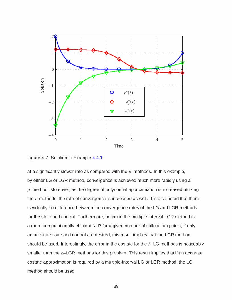
0
0
2
2 3
−1
1
1 4 5
−2
−4
−3
Sol
utio
n
Time
y∗(t)
λ∗y (t)
u∗(t)
Error
Figure 4-7. Solution to Example 4.4.1.
at a significantly slower rate as compared with the p–methods. In this example,
by either LG or LGR method, convergence is achieved much more rapidly using a
p–method. Moreover, as the degree of polynomial approximation is increased utilizing
the h-methods, the rate of convergence is increased as well. It is also noted that there
is virtually no difference between the convergence rates of the LG and LGR methods
for the state and control. Furthermore, because the multiple-interval LGR method is
a more computationally efficient NLP for a given number of collocation points, if only
an accurate state and control are desired, this result implies that the LGR method
should be used. Interestingly, the error in the costate for the h–LG methods is noticeably
smaller than the h–LGR methods for this problem. This result implies that if an accurate
costate approximation is required by a multiple-interval LG or LGR method, the LG
method should be used.
89

0
0
2
−2
−4
−6
−810050 150 200
log10
Max
imum
Err
or
Number of Collocation Points
p
h–2h–3h–4
A State Error.
0
0
2
−2
−4
−6
−810050 150 200
log10
Max
imum
Err
or
Number of Collocation Points
p
h–2h–3h–4
B Control Error.
0
0
2
−2
−4
−6
−810050 150 200
log10
Max
imum
Err
or
Number of Collocation Points
p
h–2h–3h–4
C Costate Error.
Figure 4-8. Convergence Rates Utilizing p, h–2, h–3, h–4–LG Methods for Example4.4.1.
4.4.2 Example 2 - Bryson-Denham Problem
Consider the problem to minimize the cost functional [2]
J =1
2
∫ 1
0
a2dt (4–133)
subject to the dynamic equations
x = v (4–134)
v = a (4–135)
90
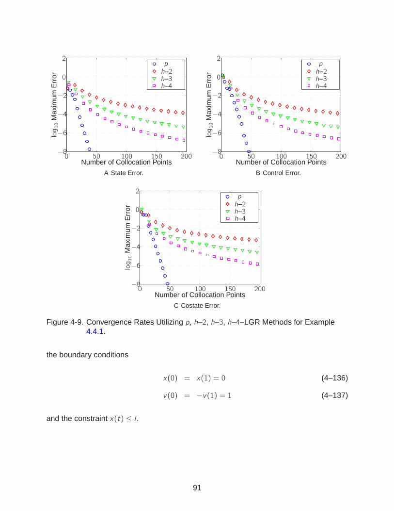
0
0
2
−2
−4
−6
−810050 150 200
log10
Max
imum
Err
or
Number of Collocation Points
ph–2h–3h–4
A State Error.
0
0
2
−2
−4
−6
−810050 150 200
log10
Max
imum
Err
or
Number of Collocation Points
ph–2h–3h–4
B Control Error.
0
0
2
−2
−4
−6
−810050 150 200
log10
Max
imum
Err
or
Number of Collocation Points
ph–2h–3h–4
C Costate Error.
Figure 4-9. Convergence Rates Utilizing p, h–2, h–3, h–4–LGR Methods for Example4.4.1.
the boundary conditions
x(0) = x(1) = 0 (4–136)
v(0) = −v(1) = 1 (4–137)
and the constraint x(t) ≤ l .
91

The solution to this problem is given as
x =
l [1− (1− t3l)3] : 0 ≤ t ≤ 3l
l : 3l ≤ t ≤ 1− 3l
l [1− (1− 1−t3l)3] : 1− 3l ≤ t ≤ 1
(4–138)
v =
(1− t3l)2 : 0 ≤ t ≤ 3l
0 : 3l ≤ t ≤ 1− 3l
−(1− 1−t3l)2 : 1− 3l ≤ t ≤ 1
(4–139)
a =
− 23l(1− t
3l) : 0 ≤ t ≤ 3l
0 : 3l ≤ t ≤ 1− 3l
− 23l(1− 1−t
3l) : 1− 3l ≤ t ≤ 1
(4–140)
λx =
29l2
: 0 ≤ t ≤ 3l
0 : 3l ≤ t ≤ 1− 3l
− 29l2: 1− 3l ≤ t ≤ 1
(4–141)
λv =
23l(1− t
3l) : 0 ≤ t ≤ 3l
0 : 3l ≤ t ≤ 1− 3l23l(1− 1−t
3l) : 1− 3l ≤ t ≤ 1
(4–142)
Unlike the previous example that had a smooth solution and a continuous costate,
the solution to this problem is only piecewise smooth and has a discontinuous costate
solution for λx . Within any piecewise interval, the highest order behavior in the exact
solution is order three. Therefore, the only difficulty in accurately approximating the
solution to this problem is in approximating the nonsmooth features at t = 3l and
92

t = 1− 3l and the fact that λx is discontinuous at t = 3l and t = 1− 3l . In this example,
l = 1/12.
4.4.2.1 Case 1: Location of Discontinuity Unknown
p–LG and LGR collocation methods and uniformly distributed h–2–LG and LGR
collocation methods are used to approximate the solution to this problem in the case
that the location of discontinuity in λx is assumed not to be known. In this case, mesh
points will, in general, not be at the location of the discontinuity in λx . Figs. 4-10A–4-10D
and Figs. 4-11A–4-11D show the convergence rates for state, control, and costate for
this problem as a function of collocation points for p and h–2–LG methods and p and
h–2–LGR methods, respectively. First, it is seen that there is essentially no difference
in the convergence rates of the p and h–2–methods. Because this problem has a
non-smooth solution, exponential convergence rates from a p–method do not exist.
Furthermore, it is seen that there is no substantial difference in accuracy between
LG and LGR methods. It is also noted that the state, control, and λv do converge
to the exact solution as the number of collocation points are increased. It is also
noted that λx does not converge as the number of collocation points are increased.
Figs. 4-12A–4-12E show the approximation for the h–2–method utilizing 150 collocation
points. Visually, the problem is reasonably approximated except for λx . The difficulty
in approximating λx is isolated to the regions near the discontinuities (i.e., the point at
approximately t = 0.25).
4.4.2.2 Case 2: Location of Discontinuity Known
Next, the solution to the problem is approximated knowing the exact locations of
discontinuities in λx . p and h–3–LG and LGR methods are used to approximate the
solution to this problem. First, define the time domains T1 ∈ [0, 3l ], T2 ∈ [3l , 1 − 3l ],
and T3 ∈ [1 − 3l , 1]. For the p–method approximations, a single approximating
interval is used for each of T1, T2, and T3 with a variable degree polynomial in each
interval. Furthermore, for the h–3–method, a variable number of uniformly distributed
93
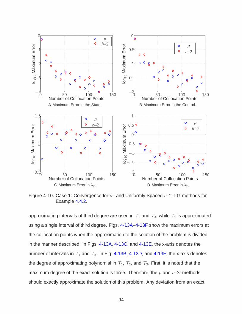
0
0
−1
−2
−410050 150
−3
log10
Max
imum
Err
or
Number of Collocation Points
p
h–2
t)
A Maximum Error in the State.
−1.5
0
0
−1
−0.5
−210050 150
log10
Max
imum
Err
or
Number of Collocation Points
p
h–2
B Maximum Error in the Control.
0
1.5
0.5
1
10050 150
plog10
Max
imum
Err
or
Number of Collocation Points
p
h–2
C Maximum Error in λx .
−1.5
0
0
−1
−0.5
0.5
1
−210050 150
log10
Max
imum
Err
or
Number of Collocation Points
p
h–2
D Maximum Error in λv .
Figure 4-10. Case 1: Convergence for p– and Uniformly Spaced h–2–LG methods forExample 4.4.2.
approximating intervals of third degree are used in T1 and T3, while T2 is approximated
using a single interval of third degree. Figs. 4-13A–4-13F show the maximum errors at
the collocation points when the approximation to the solution of the problem is divided
in the manner described. In Figs. 4-13A, 4-13C, and 4-13E, the x-axis denotes the
number of intervals in T1 and T3. In Fig. 4-13B, 4-13D, and 4-13F, the x-axis denotes
the degree of approximating polynomial in T1, T2, and T3. First, it is noted that the
maximum degree of the exact solution is three. Therefore, the p and h–3–methods
should exactly approximate the solution of this problem. Any deviation from an exact
94
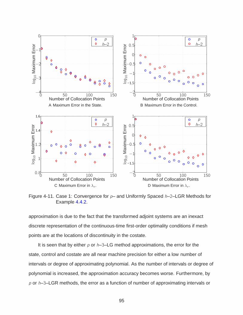
0
0
−1
−2
−410050 150
−3
log10
Max
imum
Err
or
Number of Collocation Points
p
h–2
t)
A Maximum Error in the State.
−1.5
0
0
−1
−0.5
0.5
1
−210050 150
log10
Max
imum
Err
or
Number of Collocation Points
p
h–2
B Maximum Error in the Control.
1.4
1.6
1.2
0
1
10050 1500.8
plog10
Max
imum
Err
or
Number of Collocation Points
p
h–2
C Maximum Error in λx .
−1.5
0
0
−1
−0.5
0.5
1
−210050 150
log10
Max
imum
Err
or
Number of Collocation Points
p
h–2
D Maximum Error in λv .
Figure 4-11. Case 1: Convergence for p– and Uniformly Spaced h–2–LGR Methods forExample 4.4.2.
approximation is due to the fact that the transformed adjoint systems are an inexact
discrete representation of the continuous-time first-order optimality conditions if mesh
points are at the locations of discontinuity in the costate.
It is seen that by either p or h–3–LG method approximations, the error for the
state, control and costate are all near machine precision for either a low number of
intervals or degree of approximating polynomial. As the number of intervals or degree of
polynomial is increased, the approximation accuracy becomes worse. Furthermore, by
p or h–3–LGR methods, the error as a function of number of approximating intervals or
95
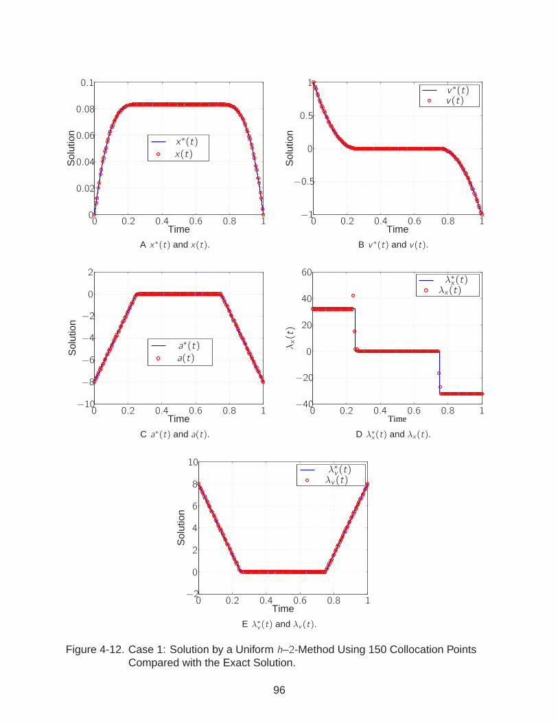
00 10.2 0.4 0.6 0.8
Sol
utio
n
Time
x∗(t)
x(t)
0.02
0.04
0.06
0.08
0.1
A x∗(t) and x(t).
0
0−1
−0.5
0.5
1
10.2 0.4 0.6 0.8
Sol
utio
n
Time
v∗(t)v(t)
B v∗(t) and v(t).
0
0
2
1
−2
−4
−6
−8
−100.2 0.4 0.6 0.8
Sol
utio
n
Time
t)
a∗(t)
a(t)
C a∗(t) and a(t).
Time
0
0 1
40
60
0.2 0.4 0.6 0.8
20
λ∗x(t)λx(t)
λx(t)
−20
−40
D λ∗x(t) and λx(t).
0
0
2
1
4
−2
6
8
10
0.2 0.4 0.6 0.8
Sol
utio
n
Time
λ∗v (t)λv (t)
E λ∗v (t) and λv (t).
Figure 4-12. Case 1: Solution by a Uniform h–2-Method Using 150 Collocation PointsCompared with the Exact Solution.
96
degree of approximating polynomial neither converges nor diverges. Rather, errors are
banded between O(10−4) and O(10−16). While high levels of accuracy are demonstrated
by p and h–3–LG and LGR methods, the behaviors of these methods with respect to
this case are erratic because the transformed adjoint system is an inexact discrete
representation of the continuous-time first-order optimality conditions.
4.5 Summary
The hp–LG and LGR pseudospectral methods for approximating a nonlinear
continuous-time optimal control problem have been posed. LG and LGR points are
used because they provide highly accurate quadrature approximations and avoid Runge
phenomenon in the Lagrange polynomial approximation of the state. Furthermore, the
hp–LG and LGR methods have been posed such that an arbitrary number of intervals,
with arbitrary location, and an arbitrary number of collocation points per interval may be
used. Over regions where the solution is smooth, increasing the number of collocation
points in approximating intervals will result in efficient high-accuracy approximations.
For regions of the trajectory where the solution is non-smooth, increasing the number of
low-order approximating intervals will result in computationally efficient approximations
of these non-smooth regions. Next, the KKT conditions of the hp–LG and LGR methods
are derived. The transformed adjoint systems are derived from the KKT conditions
and are shown to be discrete representations of the continuous-time first-order
necessary conditions if the costate is continuous. If the costate is discontinuous, then
the transformed adjoint systems are not discrete representations of the continuous-time
first-order necessary conditions. Two examples are used to demonstrate the accuracy
of approximation of the hp–LG and LGR methods. The solution to the first example
is smooth and has a continuous costate while the solution to the second example is
nonsmooth and has a discontinuous costate. It is seen in the first example that as
the number of approximating intervals or degree of approximation in any interval is
increased, the accuracy in approximating the state, control, and costate is increased as
97

−18
0
−6
−8
−10
−12
−14
−16
10 40 5020 30
LG Ptslog10
Max
imum
Err
ort)
Number of Intervals
LGR Pts
A State Error by LG and LGR h–3–Methods.
−18
0
−6
−8
−10
−12
−14
−16
10 40 5020 30
LG Pts
log10
Max
imum
Err
or
Number of Collocation Points
LGR Pts
B State Error by LG and LGR p–Methods.
0
−4
−6
−8
−10
−12
−14
−1610 40 5020 30
LG Pts
plog10
Max
imum
Err
or
Number of Intervals
LGR Pts
C Control Error by LG and LGR h–3–Methods.
0
−4
−6
−8
−10
−12
−14
−1610 40 5020 30
LG Ptslog10
Max
imum
Err
or
Number of Collocation Points
LGR Pts
D Control Error by LG and LGR p–Methods.
0
−4
−6
−8
−10
−12
−1410 40 5020 30
LG Pts
ointslog10
Max
imum
Err
or
Number of Intervals
LGR Pts
E Costate Error by LG and LGR h–3–Methods.
0
−2
−4
−6
−8
−10
−12
−1410 40 5020 30
LG Pts
log10
Max
imum
Err
or
Number of Collocation Points
LGR Pts
F Costate Error by LG and LGR p–Methods.
Figure 4-13. Case 2: Convergence for p and h–3–LG and LGR Methods for Example4.4.2.
98
well. Furthermore, there is little difference in the approximation accuracy of the state
and control using LG or LGR points, but, the costate approximation is significantly more
accurate using LG points. Next, the second example studies a problem whose solution
has a discontinuous costate. It is demonstrated that if mesh points are not located at
the location of discontinuity in the costate, significant errors exist in approximating the
discontinuity. Furthermore, if mesh points are located at the locations of discontinuity
in the costate, high levels of accuracy are obtained in the approximation although the
trends are quite erratic. For the LG methods, a few number of approximating intervals
or low-degree approximations best approximated the solution to the problem. For the
LGR methods, the errors are banded within a large range from O(10−4) to O(10−16).
Therefore, if the costate is discontinuous, it is best to put mesh points at the exact
location of discontinuity, but, guaranteeing high-accuracy by the proposed hp–LG or
LGR methods is difficult for the case of discontinuous costate solutions. Finally, the
sparsity of the hp–LG and LGR methods is studied. It is seen that as the number of
collocation points within an interval grows, so does the density of the approximating NLP.
Therefore, there is a trade off that exists between increasing the number of collocation
points in an interval in order to obtain higher accuracy solutions that also increases the
density of the NLP. If an interval is approximating a smooth region of a solution, the
rapid rates of convergence by increasing the number of LG or LGR points far outweigh
the increase in NLP density. If an interval is approximating a non-smooth region of a
solution, then it is more efficient to increase the accuracy of the approximating NLP
by dividing the problem into more low-order, sparse, approximating intervals. Finally,
it is seen that the size of the hp–LG method is dependent upon both the number of
collocation points and the number of mesh intervals whereas the size of the hp–LGR
method is only dependent upon the number of collocation points. Therefore, if a large
number of mesh intervals are to be used, the hp–LGR method results in a more efficient
NLP.
99
CHAPTER 5HP–MESH REFINEMENT ALGORITHMS
In this chapter, two hp-mesh refinement algorithms are presented using the
hp–LG and LGR methods of Chapter 4. In each algorithm, a naive initial mesh is
selected. Because it is assumed that no a priori knowledge of the solution structure
of a continuous-time optimal control problem being approximated is known, the naive
initial meshes are either a single-interval of moderate degree or relatively few uniformly
distributed intervals of low-degree. From this naive approximation, both algorithms
assess the approximation errors in each interval. If the accuracy of the approximation
in an interval needs to be improved, either the degree of approximation in the interval
is increased or the interval is subdivided into more approximating subintervals. These
strategies are then repeated iteratively until an accurate approximation is obtained.
Because a known exact solution is not generally available, solution errors in an
interval are approximated by examining how closely the differential-algebraic constraint
equations are satisfied between collocation points.
The first mesh refinement algorithm is more heavily weighted as a p–biased
hp–mesh refinement algorithm. An interval is subdivided only if it is believed that
exponential convergence does not hold in that interval. The second algorithm is an
h–biased hp–mesh refinement algorithm. In this second algorithm, subdivision of an
interval is chosen much more frequently and an increase in degree of polynomial
approximation is chosen only if the solution in an interval is considered smooth. First,
a discussion on assessment of the errors in an approximating grid are discussed.
Next, hp–mesh refinement algorithm 1 and 2 are described. It is noted that hp–mesh
refinement algorithm 1 and 2 are adaptations of the algorithms presented in Refs. [66]
and [67].
100

5.1 Approximation of Errors in a Mesh Interval
Consider an hp–LG or LGR approximation to the solution of a continuous-time
optimal control problem as defined in Chapter 4 with K mesh intervals. Furthermore,
let t0 < t1 < ... < tK be the mesh points such that tk−1 defines the beginning of
the k th mesh and tk defines the end of the k th mesh. Next, let Nk be the number of
collocation points in mesh interval k . In designing the hp–mesh refinement algorithms
an assessment of the approximation accuracy of each approximating interval k must
be made without knowledge of the exact solution to a continuous-time optimal control
problem.
In order to provide an assessment on the accuracy of the approximation without
knowledge of the exact solution, the satisfaction of the differential-algebraic constraints
between collocation points are examined. At the collocation points, the differential-algebraic
equations are enforced. However, if an approximating hp–pseudospectral approximation
is accurately approximating the continuous-time optimal control problem, then the
differential-algebraic constraints should be nearly satisfied at an arbitrary point. In
order to evaluate the differential-algebraic constraints between collocation points, the
state and control must be interpolated to an arbitrary point. The state is defined at an
arbitrary point in an interval k by the Lagrange polynomial of Eqs. (4–24) or (4–73)
for the hp–LG or LGR methods, respectively. The control on the other hand, is only
calculated at the collocation points and does not have a unique underlying polynomial
approximation. Therefore, any control approximation that matches the value of the
control at the collocation points is a valid approximation (e.g., linear, cubic, spline,
Lagrange polynomial). In this research, a Lagrange polynomial approximation of
the control is used. If the state is being approximated by a high-accuracy Lagrange
polynomial, then it is counter-productive to use a low-order, less accurate approximation
to the control. Therefore, in either the hp–LG or LGR method, the Lagrange polynomial
approximation of the control with support points at the Nk collocation points in interval k
101
is given as
U(k)(τ) =Nk∑
i=1
U(k)i L(k)i (τ). (5–1)
Using the aforementioned state and control approximations, the differential-algebraic
constraints can now be evaluated at an arbitrary point in a mesh interval k . In order to
sample the differential-algebraic constraints between the collocation points, define
L points in interval k as t(k) = (t(k)1 , ... , t(k)L ) ∈ [tk−1, tk ]. The differential-algebraic
constraints can then be evaluated at these L points as
∣
∣
∣X(k)i (t
(k)l )− f
(k)i (X
(k)l ,U
(k)l )
∣
∣
∣= a
(k)li , (5–2)
C(k)j (X
(k)l ,U
(k)l ) = b
(k)lj , (5–3)
where i = 1, ... , n, j = 1, ... , s , and l = 1, ... ,L. Next, define e(k)max as the maximum
element of a(k)li or b(k)lj . If e(k)max is less than a specified error tolerance, ǫ, then the solution
in the interval is considered accurate. It is noted that Eq. (5–2) is the magnitude of
the violation in the collocation equations while Eq. (5–3) is simply an evaluation of the
inequality path constraints at L points. If the inequality path constraints are inactive,
the left hand side of Eq. (5–3) will be negative, and therefore, be less than ǫ. When the
path constraints are active, between collocation points the left hand side of Eq. (5–3)
may become positive thus violating the path constraint. If any element a(k)li or b(k)lj is
greater than ǫ, then the interval is considered inaccurate and must be refined such
that a more accurate approximation is made. The two hp–mesh refinement algorithms
are now presented that determine how to refine inaccurate approximating intervals. In
hp–mesh refinement algorithm 1, the errors estimated in Eqs. (5–2)–(5–3) are used
directly to determine if an inaccurate interval should be subdivided or if the degree of
approximation should be increased. In hp–mesh refinement algorithm 2, an h–biased
strategy is used. The curvature of the state in an interval is used to determine the
placement of the mesh points and whether to subdivide an interval or increase the
degree of the approximating polynomial within an interval. Even when it is chosen to
102
increase the degree of the approximating polynomial, the degree of the approximation
remains small.
5.2 hp–Mesh Refinement Algorithm 1
A description of hp–mesh refinement algorithm 1 is now given. It is noted that
hp–mesh refinement algorithm 1 is similar to the algorithm presented in Ref. [66] except
for the following differences. In Ref. [66], a cubic interpolation to the control was used.
In this dissertation, a Lagrange polynomial approximation to the control is used within
each interval. Furthermore, in Ref. [66], errors are assessed at the midpoints between
collocation points, whereas in this dissertation, errors are assessed at the arbitrary
points t(k) within each interval. Furthermore, Ref. [66] only modified the mesh based
upon analysis of the collocation conditions. In this dissertation, the collocation conditions
and path constraints are used to modify the mesh.
5.2.1 Increasing Degree of Approximation or Subdividing
The fundamental and distinct property of an hp–mesh refinement algorithm is the
step that determines whether to increase the degree of polynomial approximation in an
inaccurate interval or to subdivide the interval. Consider again the matrices defining the
violation of the differential-algebraic constraint equations in Eqs. (5–2) and (5–3)
A(k) = a(k)li (5–4)
B(k) = b(k)lj , (5–5)
where the column i of A(k) and column j of B(k) defines the magnitude of violation
in the collocation equations for the i th component of the state and violation of the j th
path constraint equation, respectively, at t(k). Let the state X (k)m (t), m ∈ [1, n] be the
component of the state approximation with the maximum value of a(k)li . Furthermore,
let the constraint C (k)p p ∈ [1, s] be the pth inequality path constraint with the maximum
value of b(k)lj . The component of the state or inequality path constraint with maximum
error is always used to determine how to proceed with the mesh refinement. If e(k)max is
103
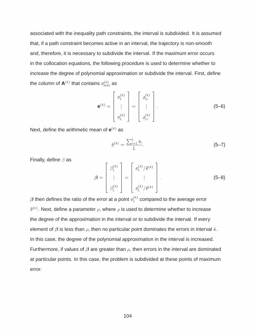
associated with the inequality path constraints, the interval is subdivided. It is assumed
that, if a path constraint becomes active in an interval, the trajectory is non-smooth
and, therefore, it is necessary to subdivide the interval. If the maximum error occurs
in the collocation equations, the following procedure is used to determine whether to
increase the degree of polynomial approximation or subdivide the interval. First, define
the column of A(k) that contains e(k)max as
e(k) =
e(k)1
...
e(k)L
=
a(k)1i
...
a(k)Li
. (5–6)
Next, define the arithmetic mean of e(k) as
e(k) =
∑L
i=1 ei
L. (5–7)
Finally, define β as
β =
β(k)1...
β(k)L
=
e(k)1 /e(k)
...
e(k)L /e(k)
. (5–8)
β then defines the ratio of the error at a point e(k)1 compared to the average error
e(k). Next, define a parameter ρ, where ρ is used to determine whether to increase
the degree of the approximation in the interval or to subdivide the interval. If every
element of β is less than ρ, then no particular point dominates the errors in interval k .
In this case, the degree of the polynomial approximation in the interval is increased.
Furthermore, if values of β are greater than ρ, then errors in the interval are dominated
at particular points. In this case, the problem is subdivided at these points of maximum
error.
104
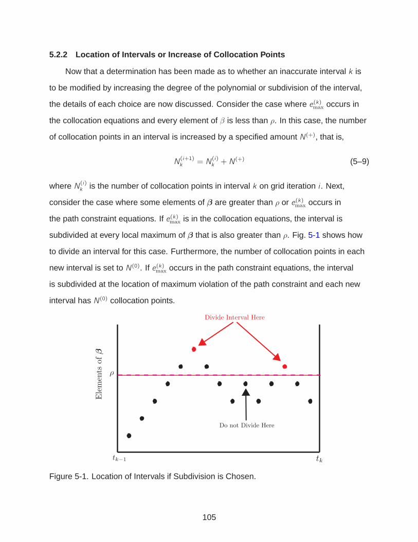
5.2.2 Location of Intervals or Increase of Collocation Poin ts
Now that a determination has been made as to whether an inaccurate interval k is
to be modified by increasing the degree of the polynomial or subdivision of the interval,
the details of each choice are now discussed. Consider the case where e(k)max occurs in
the collocation equations and every element of β is less than ρ. In this case, the number
of collocation points in an interval is increased by a specified amount N(+), that is,
N(i+1)k = N
(i)k + N
(+) (5–9)
where N(i)k is the number of collocation points in interval k on grid iteration i . Next,
consider the case where some elements of β are greater than ρ or e(k)max occurs in
the path constraint equations. If e(k)max is in the collocation equations, the interval is
subdivided at every local maximum of β that is also greater than ρ. Fig. 5-1 shows how
to divide an interval for this case. Furthermore, the number of collocation points in each
new interval is set to N(0). If e(k)max occurs in the path constraint equations, the interval
is subdivided at the location of maximum violation of the path constraint and each new
interval has N(0) collocation points.
-
Figure 5-1. Location of Intervals if Subdivision is Chosen.
105

5.2.3 Stopping Criteria
The algorithm stops when the dynamic constraints and inequality path constraints
are satisfied to the tolerance ǫ in every interval at L points between the collocation
points.
5.2.4 hp–Mesh Refinement Algorithm 1
hp–Mesh Refinement Algorithm 1 is now stated.
1. If this is the first iteration, initialize the problem choosing N(0) collocation points andK = 1 number of intervals, where N(0) is chosen by the user. Otherwise, solve theNLP using the current mesh.Begin: For k = 1, ... ,K ,
2. If e(k)max ≤ ǫ, then do not modify interval k . Otherwise, continue to step 3.
3. If the maximum error occurs in the collocation equations and every elementof β(k) < ρ, then increase the degree of approximation of mesh interval k byN(+).
4. Otherwise, if errors are largest in the collocation equations, refine the intervalat the points defining the maximum errors in β. If errors are largest in thepath constraint equations, refine the interval at the point of maximum error.Furthermore, set the number of collocation points to N(0) = 5 in each newinterval.
End: For k = 1, ... ,K .
5. Return to Step 1.
Several important aspects of hp–mesh refinement algorithm 1 are now clarified. It
is noted that ρ serves as a tuning parameter that varies the amount of weighting from
h to p–biases. For very small values of ρ, the h–bias is increased. For large values of
ρ, the algorithm is more p–biased. ρ should be selected such that detection of large
isolated errors is made and the approximation can be subdivided about these points.
Next, for the problems analyzed in this dissertation, N(+) = 10 because increasing
by more than ten collocation points may make the NLP unnecessarily dense. Next, all
newly created intervals are initialized with five collocation points for two reasons. First,
if exponential convergence in a newly created interval holds, five collocation points may
106

provide high-accuracy solutions. Second, initializing a newly created interval with five
collocation points will keep the total number of collocation points small.
5.3 hp–Mesh Refinement Algorithm 2
hp–mesh refinement algorithm 2 is now defined. Different from hp–mesh refinement
algorithm 1, hp–mesh refinement algorithm 2 is designed to be a much more h–biased
algorithm. It is noted that hp–mesh refinement algorithm 2 is similar to the algorithm
presented in Ref. [67] with the only modification in this dissertation being how the control
is interpolated. In this dissertation, the control in interval k ∈ 1, ... ,K is interpolated by
a Lagrange polynomial using support points at the Nk collocation points. In Ref. [67],
the control is interpolated with a Lagrange polynomial with support points at the Nk
collocation points and one additional non-collocated point for k ∈ 1, ... ,K − 1 and by a
Lagrange polynomial with support points at the NK collocation points in the final interval
K .
5.3.1 Increasing Degree of Approximation or Subdividing
If the solution in a mesh interval k is inaccurate, the first determination is whether
the degree of approximation in the interval should be increased or whether the interval
should be subdivided. Suppose that X (k)m (τ) is the component of the state approximation
in the k th mesh interval that corresponds to the maximum value of a(k)li . Furthermore, let
the curvature of the mth component of the state in mesh interval k be given by
κ(k)(τ) =|X (k)m (τ)|
∣
∣
∣
∣
[
1 + X(k)m (τ)2
]3/2∣
∣
∣
∣
. (5–10)
Next, define κ(k)max and κ(k) be the maximum and mean value of κ(k)(τ), respectively.
Furthermore, let rk be the ratio of the maximum to the mean curvature:
rk =κ(k)maxκ(k). (5–11)
107

If rk < rmax, where rmax > 0 is a user-defined parameter, then the curvature of mesh
interval k is considered uniform and the degree of approximation is increased within the
interval. If rk > rmax, then a large curvature relative to the remainder of the interval exists
and the interval is subdivided.
5.3.2 Increase in Polynomial Degree in Interval k
If rk < rmax, then the polynomial degree in mesh interval k needs to be increased.
Let M be the current degree of the approximating polynomial in the interval. The degree
Nk of the polynomial for the next grid iteration in mesh interval k is given by the formula
Nk = M + ceil(log10(e(k)max/ǫ)) + A (5–12)
where A > 0 is an arbitrary integer constant and ceil is the operator that rounds to the
next highest integer.
5.3.3 Determination of Number and Placement of New Mesh Point s
If rk > rmax, then mesh interval k is subdivided. Two quantities are now defined: The
number of subdivisions and the location of each subdivision. First, the new number of
mesh intervals, denoted nk , is computed as
nk = ceil(B log10(e(k)max/ǫ)), (5–13)
where B is an arbitrary integer constant. The locations of the new mesh points are
determined using the integral of a curvature density function in a manner similar to that
given in Ref. [30]. Specifically, let ρ(τ) be the density function [30] given by
ρ(τ) = cκ(τ)1/3, (5–14)
where c is a constant chosen so that
∫ +1
−1
ρ(ζ)dζ = 1.
108
Let F (τ) be the cumulative distribution function given by
F (τ) =
∫ τ
−1
ρ(ζ)dζ. (5–15)
The nk new mesh points are chosen so that
F (τi) =i − 1nk, 1 ≤ i ≤ nk + 1.
It is shown in Ref. [30] that placing the mesh points in this manner is results in the
smallest L1 norm error when a piecewise linear approximation of a curve is used. Finally,
it is noted that if nk = 1, then no subintervals are created. Therefore, the minimum value
for nk should be at least two. Figs. 5-2A and 5-2B show qualitatively how to divide an
interval into more intervals for a constant curvature in an interval and an interval with a
large curvature relative to the remainder of the interval, respectively.
5.4 hp–Mesh Refinement Algorithm 2
hp–mesh refinement algorithm 2 is now defined. The algorithm is initialized for a
coarse uniformly distributed mesh with a fixed, low-degree polynomial in each interval.
This approximation is solved, and then each mesh interval is analyzed. If errors are
less than ǫ, then the interval is not modified. Otherwise, if errors are greater than ǫ,
then the interval is modified according to the discussion of Sections 5.1 through 5.3.3.
The refinement process continues iteratively until a suitable approximating mesh is
constructed. hp–mesh refinement algorithm 2 is now given:
1. Solve the NLP using the current mesh.Begin: For k = 1, ... ,K ,
2. If e(k)max ≤ ǫ, do not modify interval k .
3. If either rk ≥ rmax or Nk > M, then refine the k th mesh interval into nksubintervals where nk is given by (5–13). Set the degree of the polynomialson each of the subintervals to be M and proceed to the next k .
4. Otherwise, set the degree of the polynomials on the k th subinterval to be Nk ,which is given in (5–12).
End: For k = 1, ... ,K .
109

A Constant Curvature.
B Variable Curvature.
Figure 5-2. Location of Intervals based on Curvature.
5. Return to Step 1.
Several important aspects of hp–mesh refinement algorithm 2 are now clarified.
hp–mesh refinement algorithm 2 is a h–biased algorithm. It is noted that unlike hp–mesh
refinement algorithm 1, an increase in the degree of polynomial approximation is
only allowed once within an interval. If the errors in approximation are still large after
increasing the degree of approximation, the interval is forced to subdivide as opposed
to increasing the degree of approximation again. Furthermore, Eq. (5–12) defines the
number of collocation points that are added to an interval based on a log10 difference in
110
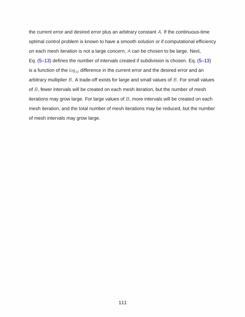
the current error and desired error plus an arbitrary constant A. If the continuous-time
optimal control problem is known to have a smooth solution or if computational efficiency
on each mesh iteration is not a large concern, A can be chosen to be large. Next,
Eq. (5–13) defines the number of intervals created if subdivision is chosen. Eq. (5–13)
is a function of the log10 difference in the current error and the desired error and an
arbitrary multiplier B. A trade-off exists for large and small values of B. For small values
of B, fewer intervals will be created on each mesh iteration, but the number of mesh
iterations may grow large. For large values of B, more intervals will be created on each
mesh iteration, and the total number of mesh iterations may be reduced, but the number
of mesh intervals may grow large.
111

CHAPTER 6EXAMPLES
The hp–mesh refinement algorithms posed in Chapter 5 are now examined on
a variety of optimal control problems. The first example is the motivating example
of Section 3.1 whose solution, as we recall, is smooth. The second example is a
reusable launch vehicle entry problem whose solution appears to be smooth. The third
example is a problem where the timescale of the dynamics become fast as the final time
increases. The fourth example is the motivating example of Section 3.2 whose solution,
as we recall, is not smooth. Finally, the fifth example is a minimum time-to-climb of
a supersonic aircraft. This final example has two active path constraints along the
trajectory. The objective of this Chapter is to assess how well the hp–mesh refinement
algorithms perform relative to p and h–methods.
The examples were solved with modifications of the open-source optimal control
software GPOPS [37] using the NLP solver SNOPT [68]. All computations were
performed using a 2.5 GHZ Core 2 Duo Macbook Pro running Mac OS-X 10.5.8 with
MATLAB R2009b. Furthermore, analytic derivatives were used in the NLP solver. The
p–method discretizations were solved utilizing a single approximating interval with a
variable number of collocation points in the interval. The p–method simply assesses
the violations of Eqs. (5–2)–(5–3) at L uniformly distributed points between collocation
points where L = 1000. If errors are greater than ǫ, the number of collocation points
is increased by ten. Next, hp–mesh refinement algorithm 1 (hp(1)) uses ρ = 3.5 and
evaluates in each interval the violations of Eqs. (5–2)–(5–3) at L = 100 uniformly
distributed points between collocation points. hp–mesh refinement algorithm 2 (hp(2))
uses rmax = 2, A = 1, B = 2, and L = 30 uniformly distributed points between collocation
points. Finally, the h–method is an adaptation of hp–mesh refinement algorithm 2. For
the h–method, hp–mesh refinement algorithm 2 is used with rmax < 1, permitting only
segment division and preventing growth in the degree of the approximating polynomial.
112

The terminology “h–x–” denotes an h–method with x number of collocation points
in each interval while “hp(2)–x–” denotes the hp(2)–method with a minimum of x
collocation points in each interval. All examples were solved utilizing LGR points.
Finally, a maximum limit of 200 collocation points is given for the p–method. If a suitable
approximation is not obtained for 200 collocation points, then it is decided that an
accurate approximation cannot be obtained. Furthermore, for the hp(1), hp(2), and
h–methods, a mesh iteration limit of 40 is given. If a suitable approximation is not found
within 40 mesh iterations, then it is decided that an accurate approximation cannot be
obtained.
6.1 Example 1 - Motivating Example 1
Consider again the motivating example given by Eqs. (3–1)–(3–3). The problem is
now restated. Minimize the cost functional
J = tf (6–1)
subject to the dynamic constraints
x = cos(θ) , y = sin(θ) , θ = u, (6–2)
and the boundary conditions
x(0) = 0 , y(0) = 0 , θ(0) = −π
x(tf ) = 0 , y(tf ) = 0 , θ(tf ) = π.(6–3)
The solution to the optimal control problem of Eqs. (6–1)–(6–3) is
(x∗(t), y ∗(t), θ∗(t), u∗(t)) = (− sin(t),−1 + cos(t), t − π, 1) (6–4)
where t∗f = 2π. As was demonstrated in Section 3.1, a p–method results in most
efficient approximation to this problem. Therefore, it is expected that the p and hp(1)
strategies will perform the best. Table 6-1 shows the initial uniformly distributed grid for
each strategy studied and the number of collocation points in each interval. It is noted
113
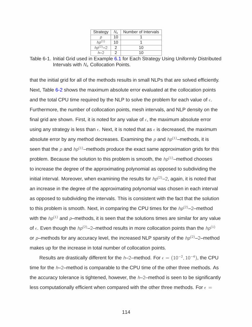
Strategy Nk Number of Intervalsp 10 1hp(1) 10 1hp(2)–2 2 10h–2 2 10
Table 6-1. Initial Grid used in Example 6.1 for Each Strategy Using Uniformly DistributedIntervals with Nk Collocation Points.
that the initial grid for all of the methods results in small NLPs that are solved efficiently.
Next, Table 6-2 shows the maximum absolute error evaluated at the collocation points
and the total CPU time required by the NLP to solve the problem for each value of ǫ.
Furthermore, the number of collocation points, mesh intervals, and NLP density on the
final grid are shown. First, it is noted for any value of ǫ, the maximum absolute error
using any strategy is less than ǫ. Next, it is noted that as ǫ is decreased, the maximum
absolute error by any method decreases. Examining the p and hp(1)–methods, it is
seen that the p and hp(1)–methods produce the exact same approximation grids for this
problem. Because the solution to this problem is smooth, the hp(1)–method chooses
to increase the degree of the approximating polynomial as opposed to subdividing the
initial interval. Moreover, when examining the results for hp(2)–2, again, it is noted that
an increase in the degree of the approximating polynomial was chosen in each interval
as opposed to subdividing the intervals. This is consistent with the fact that the solution
to this problem is smooth. Next, in comparing the CPU times for the hp(2)–2–method
with the hp(1) and p–methods, it is seen that the solutions times are similar for any value
of ǫ. Even though the hp(2)–2–method results in more collocation points than the hp(1)
or p–methods for any accuracy level, the increased NLP sparsity of the hp(2)–2–method
makes up for the increase in total number of collocation points.
Results are drastically different for the h–2–method. For ǫ = (10−2, 10−4), the CPU
time for the h–2–method is comparable to the CPU time of the other three methods. As
the accuracy tolerance is tightened, however, the h–2–method is seen to be significantly
less computationally efficient when compared with the other three methods. For ǫ =
114
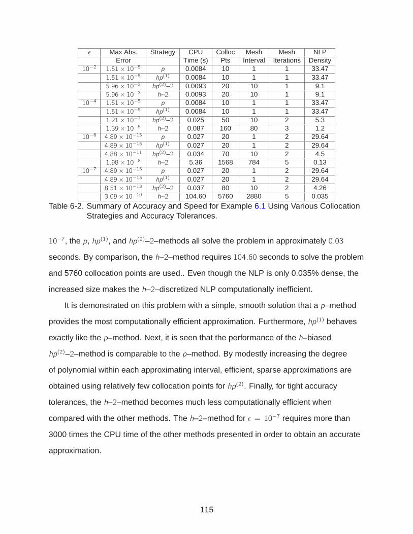
ǫ Max Abs. Strategy CPU Colloc Mesh Mesh NLPError Time (s) Pts Interval Iterations Density
10−2 1.51× 10⁻⁵ p 0.0084 10 1 1 33.471.51× 10−5 hp(1) 0.0084 10 1 1 33.475.96× 10−3 hp(2)–2 0.0093 20 10 1 9.15.96× 10−3 h–2 0.0093 20 10 1 9.1
10−4 1.51× 10⁻⁵ p 0.0084 10 1 1 33.471.51× 10−5 hp(1) 0.0084 10 1 1 33.471.21× 10−7 hp(2)–2 0.025 50 10 2 5.31.39× 10−5 h–2 0.087 160 80 3 1.2
10−6 4.89× 10⁻¹⁵ p 0.027 20 1 2 29.644.89× 10−15 hp(1) 0.027 20 1 2 29.644.88× 10−11 hp(2)–2 0.034 70 10 2 4.51.98× 10−8 h–2 5.36 1568 784 5 0.13
10−7 4.89× 10⁻¹⁵ p 0.027 20 1 2 29.644.89× 10−15 hp(1) 0.027 20 1 2 29.648.51× 10−13 hp(2)–2 0.037 80 10 2 4.263.09× 10−10 h–2 104.60 5760 2880 5 0.035
Table 6-2. Summary of Accuracy and Speed for Example 6.1 Using Various CollocationStrategies and Accuracy Tolerances.
10−7, the p, hp(1), and hp(2)–2–methods all solve the problem in approximately 0.03
seconds. By comparison, the h–2–method requires 104.60 seconds to solve the problem
and 5760 collocation points are used.. Even though the NLP is only 0.035% dense, the
increased size makes the h–2–discretized NLP computationally inefficient.
It is demonstrated on this problem with a simple, smooth solution that a p–method
provides the most computationally efficient approximation. Furthermore, hp(1) behaves
exactly like the p–method. Next, it is seen that the performance of the h–biased
hp(2)–2–method is comparable to the p–method. By modestly increasing the degree
of polynomial within each approximating interval, efficient, sparse approximations are
obtained using relatively few collocation points for hp(2). Finally, for tight accuracy
tolerances, the h–2–method becomes much less computationally efficient when
compared with the other methods. The h–2–method for ǫ = 10−7 requires more than
3000 times the CPU time of the other methods presented in order to obtain an accurate
approximation.
115
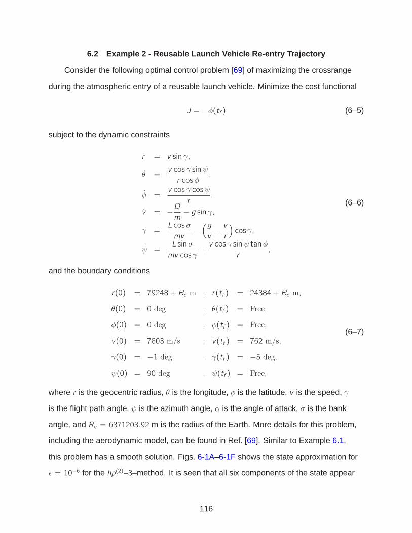
6.2 Example 2 - Reusable Launch Vehicle Re-entry Trajectory
Consider the following optimal control problem [69] of maximizing the crossrange
during the atmospheric entry of a reusable launch vehicle. Minimize the cost functional
J = −φ(tf ) (6–5)
subject to the dynamic constraints
r = v sin γ,
θ =v cos γ sinψ
r cosφ,
φ =v cos γ cosψ
r,
v = −Dm
− g sin γ,
γ =L cos σ
mv−
(g
v− vr
)
cos γ,
ψ =L sinσ
mv cos γ+v cos γ sinψ tanφ
r,
(6–6)
and the boundary conditions
r(0) = 79248 + Re m , r(tf ) = 24384 + Re m,
θ(0) = 0 deg , θ(tf ) = Free,
φ(0) = 0 deg , φ(tf ) = Free,
v(0) = 7803 m/s , v(tf ) = 762 m/s,
γ(0) = −1 deg , γ(tf ) = −5 deg,
ψ(0) = 90 deg , ψ(tf ) = Free,
(6–7)
where r is the geocentric radius, θ is the longitude, φ is the latitude, v is the speed, γ
is the flight path angle, ψ is the azimuth angle, α is the angle of attack, σ is the bank
angle, and Re = 6371203.92 m is the radius of the Earth. More details for this problem,
including the aerodynamic model, can be found in Ref. [69]. Similar to Example 6.1,
this problem has a smooth solution. Figs. 6-1A–6-1F shows the state approximation for
ǫ = 10−6 for the hp(2)–3–method. It is seen that all six components of the state appear
116

to be smooth. Therefore, it is expected that a p–biased method will provide the most
computationally efficient approximations to this problem.
Table 6-3 shows the initial uniform grid and number of collocation points in each
interval for each of the methods studied. Next, Table 6-4 shows the results for each
method for various values of ǫ. For ǫ = 10−4, all methods perform comparably with a
slight advantage to the hp(2)–x– and h–2–methods. It is noted for this problem, unlike
the previous problem, the hp(1)–method does not increase the degree of approximation
from the initial interval, but instead, actually subdivides the initial interval into three
subintervals of five collocation points each that satisfy the accuracy criterion ǫ = 10−4.
For ǫ = 10−6, the hp(1) method, interestingly, performs the worst with respect to CPU
time. It is noted, however, that hp(1) also requires the most mesh iterations to obtain
a solution. Furthermore, it is noted that although the p–method results in the fewest
number of collocation points, it is not the most computationally efficient method for
ǫ = 10−6. The reduction in computational efficiency of the p–method is due to the fact
that the p–method NLP density for this problem is significantly greater than either the
hp(2)–x– or h–2–method NLP densities. Interestingly, the hp(2)–x and h–2–methods are
the most computationally efficient for ǫ = 10−6.
For ǫ = (10−7, 10−8), the h–2–method is significantly slower than the other methods.
Because of the large problem size, the resulting NLP becomes computationally
intractable. In comparing the p, hp(1) and hp(2)–x–methods, it is seen again that the hp(1)
method requires the greatest computational time because it requires the most number
of mesh iterations. For ǫ = 10−8, the p–method provides the fastest computational
speeds. For this problem, for very high levels of accuracy, the p–method is the most
computationally efficient. Next, in comparing the hp(2)–x–methods, it is seen that the
hp(2)–3 and hp(2)–4–methods perform twice as fast as the hp(2)–2–method. An increase
in one or two collocation points for high levels of accuracy, therefore, strongly affect the
CPU times by reducing the overall size of the problem for ǫ = 10−8. Finally, it is noted for
117
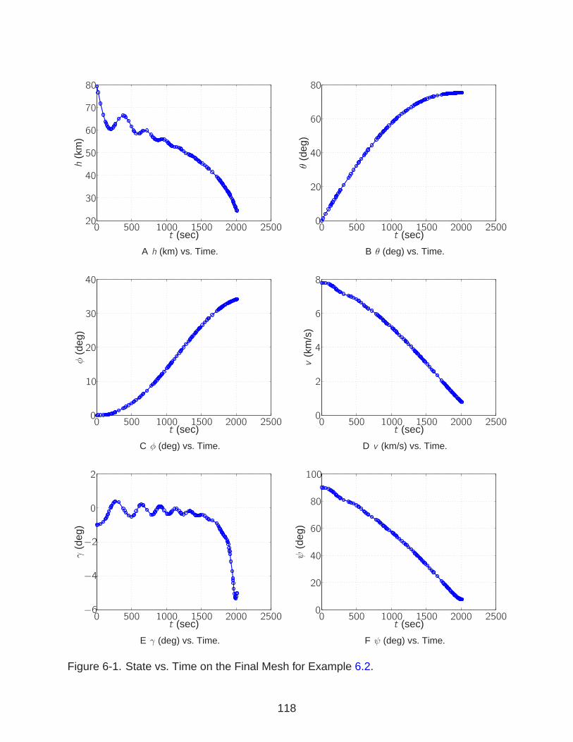
0
40
60
80
50
20
30
1000 2000500
70
1500 2500t (sec)
h(k
m)
A h (km) vs. Time.
00
40
60
80
20
1000 2000500 1500 2500t (sec)
θ(d
eg)
B θ (deg) vs. Time.
00
10
40
20
30
1000 2000
4985
500 1500 2500t (sec)
φ(d
eg)
C φ (deg) vs. Time.
00
2
4
6
8
1000 2000500 1500 2500t (sec)
v(k
m/s
)
D v (km/s) vs. Time.
0
0
2
−2
−4
−61000 2000500 1500 2500t (sec)
γ(d
eg)
E γ (deg) vs. Time.
00
40
60
80
100
20
1000 2000500 1500 2500t (sec)
ψ(d
eg)
F ψ (deg) vs. Time.
Figure 6-1. State vs. Time on the Final Mesh for Example 6.2.
118
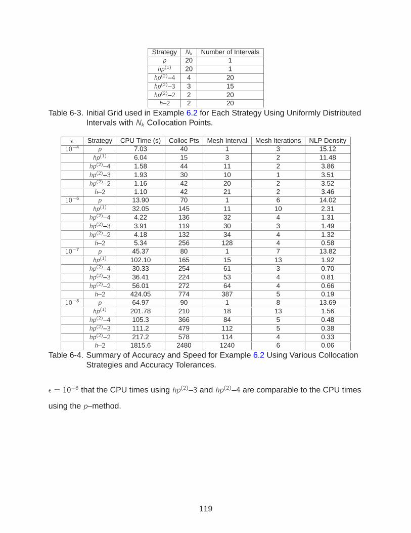
Strategy Nk Number of Intervalsp 20 1hp(1) 20 1hp(2)–4 4 20hp(2)–3 3 15hp(2)–2 2 20h–2 2 20
Table 6-3. Initial Grid used in Example 6.2 for Each Strategy Using Uniformly DistributedIntervals with Nk Collocation Points.
ǫ Strategy CPU Time (s) Colloc Pts Mesh Interval Mesh Iterations NLP Density10−4 p 7.03 40 1 3 15.12
hp(1) 6.04 15 3 2 11.48hp(2)–4 1.58 44 11 2 3.86hp(2)–3 1.93 30 10 1 3.51hp(2)–2 1.16 42 20 2 3.52h–2 1.10 42 21 2 3.46
10−6 p 13.90 70 1 6 14.02hp(1) 32.05 145 11 10 2.31hp(2)–4 4.22 136 32 4 1.31hp(2)–3 3.91 119 30 3 1.49hp(2)–2 4.18 132 34 4 1.32h–2 5.34 256 128 4 0.58
10−7 p 45.37 80 1 7 13.82hp(1) 102.10 165 15 13 1.92hp(2)–4 30.33 254 61 3 0.70hp(2)–3 36.41 224 53 4 0.81hp(2)–2 56.01 272 64 4 0.66h–2 424.05 774 387 5 0.19
10−8 p 64.97 90 1 8 13.69hp(1) 201.78 210 18 13 1.56hp(2)–4 105.3 366 84 5 0.48hp(2)–3 111.2 479 112 5 0.38hp(2)–2 217.2 578 114 4 0.33h–2 1815.6 2480 1240 6 0.06
Table 6-4. Summary of Accuracy and Speed for Example 6.2 Using Various CollocationStrategies and Accuracy Tolerances.
ǫ = 10−8 that the CPU times using hp(2)–3 and hp(2)–4 are comparable to the CPU times
using the p–method.
119

6.3 Example 3: Hyper-Sensitive Problem
Consider the following hyper-sensitive [70–73] optimal control problem adapted from
Ref. [71]. Minimize the cost functional
J =1
2
∫ tf
0
(x2 + u2)dt (6–8)
subject to the dynamic constraint
x = −x3 + u (6–9)
and the boundary conditions
x(0) = 1 , x(tf ) = 1 (6–10)
where tf is fixed. This problem is the final example problem considered in this Chapter
whose solution is smooth. This problem has a “take-off’,” “cruise,” and “landing” structure
where all of the interesting behavior occurs in the “take-off” and “landing” segments
(i.e., the first ten and last ten time units of the solution). For further details, Ref. [71]
contains a more in-depth discussion of this problem. The solution to this problem is now
approximated for three different values of tf .
6.3.1 Solutions for tf = 50
The problem defined by Eqs. (6–8)–(6–10) is now studied for tf = 50. The initial
approximating grids are defined in Table 6-5 and results for the various approximation
methods are given in Table 6-6. The approximation to the state and control of this
problem for tf = 50 is shown for the hp(2)–2–approximation with ǫ = 10−4 in Figs. 6-2A
and 6-2B. It is seen that in Figs. 6-2A and 6-2B, the initial mesh during the “cruise”
segment was not modified. The only refinement that occurred was to more accurately
approximate the “take-off” and “landing” segments. Next, it is interesting to note, that
while the solution to this problem is smooth, the p–method was not able to obtain a
solution for ǫ = 10−6. Furthermore, each method has a similar CPU time for ǫ =
(10−2, 10−4). As with the previous two examples, for the tightest accuracy tolerance,
120

Strategy Nk Number of Intervalsp 10 1hp(1) 10 1hp(2)–4 10 4hp(2)–3 10 3hp(2)–2 10 2h–2 10 2
Table 6-5. Initial Grid used in Example 6.3.1 for Each Strategy Using UniformlyDistributed Intervals with Nk Collocation Points.
ǫ Strategy CPU Time (s) Colloc Pts Mesh Interval Mesh Iterations NLP Density10−2 p 0.11 30 1 3 50.69
hp(1) 0.25 15 3 3 24.42hp(2)–4 0.12 56 14 3 6.75hp(2)–3 0.14 35 11 4 9.52hp(2)–2 0.15 30 14 4 9.43h–2 0.24 34 17 6 8.06
10−4 p 0.33 60 1 6 50.38hp(1) 1.01 55 7 7 12.37hp(2)–4 0.25 86 20 3 4.75hp(2)–3 0.31 74 20 4 5.19hp(2)–2 0.24 65 21 4 5.71h–2 0.69 162 81 6 1.82
10−6 p 7.74∗ 200∗ 1∗ 20∗ 50.12∗
hp(1) 2.15 100 10 9 7.98hp(2)–4 0.96 168 36 6 2.61hp(2)–3 1.26 147 31 6 3.08hp(2)–2 0.80 129 28 5 3.58h–2 74.15 1328 664 7 0.22
Table 6-6. Summary of Accuracy and Speed for Example 6.3.1 Using VariousCollocation Strategies and Accuracy Tolerances.
the h–2–method requires significantly more computational time in order to obtain an
accurate approximation when compared with the hp–methods. Furthermore, unlike
the previous two examples, the p–method is unable to obtain a solution for the tightest
accuracy tolerance. For this example, in order to obtain an efficient high-accuracy
solution, an hp–method is required.
6.3.2 Solutions for tf = 1000
The problem defined by Eqs. (6–8)–(6–10) is now examined for tf = 1000 with the
initial approximating grids defined in Table 6-7 and results for the various approximation
methods given in Table 6-8. First, the p–method is the most computationally inefficient
121
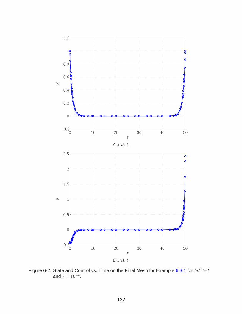
0
0
1
10 40 5020 30−0.2
0.2
0.4
0.6
0.8
1.2
x
t
A x vs. t.
0
0
1.5
2
2.5
−0.5
0.5
1
10 40 5020 30t
u
B u vs. t.
Figure 6-2. State and Control vs. Time on the Final Mesh for Example 6.3.1 for hp(2)–2and ǫ = 10−4.
122

Strategy Nk Number of Intervalsp 10 1hp(1) 10 1hp(2)–4 10 4hp(2)–3 10 3hp(2)–2 10 2h–2 10 2
Table 6-7. Initial Grid used in Example 6.3.2 for Each Strategy Using UniformlyDistributed Intervals with Nk Collocation Points.
approximation for the lowest accuracy tolerance. The number of collocation points
for the p–method approximation is larger than the hp(1), hp(2)–x , and h–2–methods.
Furthermore, the NLP density of the p–method is much greater than any of the other
methods. Therefore, the p–method is the most computationally inefficient method.
Next, it is seen that the p–method is unable to obtain an approximation for the accuracy
tolerances of ǫ = (10−4, 10−6).
Finally, in studying the h–2 approximations, for ǫ = (10−2, 10−4), the h–2–method
performs similarly when compared with the hp–methods. Again it is noted for the
tightest accuracy tolerance, the h–2–method is significantly more inefficient, requiring
approximately 170 seconds to solve the problem using 9 mesh iterations and 664
approximating intervals on the final mesh. The hp–methods, however, required
approximately five seconds to solve the problem for ǫ = 10−6. For tf = 1000, again,
high-accuracy efficient solutions are only obtained by the hp–methods.
6.3.3 Solutions for tf = 5000
Finally, the problem is analyzed for tf = 5000 with the initial approximating grids
given by Table 6-9 and results given in Table 6-10. It is noted that for the p–method
approximation, L = 10000 in order to increase the resolution of the error assessment.
For this problem, the p–method is unable to obtain a solution for any value of ǫ. It is
again seen that for ǫ = (10−2, 10−4), the hp and h–methods perform comparably, and
for the tightest accuracy tolerance, the h–2–method again is much less computationally
efficient.
123

ǫ Strategy CPU Time (s) Colloc Pts Mesh Interval Mesh Iterations NLP Density10−2 p 8.56 90 1 9 50.26
hp(1) 0.71 30 6 5 13.49hp(2)–4 0.12 56 14 3 6.75hp(2)–3 0.27 56 18 6 6.06hp(2)–2 0.27 38 18 6 7.53h–2 0.37 46 23 8 6.10
10−4 p 9.53∗ 200∗ 1∗ 20∗ 50.12∗
hp(1) 1.97 70 10 8 9.05hp(2)–4 0.25 86 20 3 4.75hp(2)–3 1.17 141 43 7 2.57hp(2)–2 0.66 104 37 8 3.42h–2 1.03 184 92 8 1.60
10−6 p – – – – –hp(1) 4.05 125 15 9 5.84hp(2)–4 4.71 214 46 6 2.06hp(2)–3 5.93 246 59 7 1.73hp(2)–2 2.97 209 53 8 2.08h–2 169.55 1328 664 9 0.22
Table 6-8. Summary of Accuracy and Speed for Example 6.3.2 Using VariousCollocation Strategies and Accuracy Tolerances.
Strategy Nk Number of Intervalsp 10 1hp(1) 10 1hp(2)–4 10 4hp(2)–3 10 3hp(2)–2 10 2h–2 10 2
Table 6-9. Initial Grid used in Example 6.3.3 for Each Strategy Using UniformlyDistributed Intervals with Nk Collocation Points.
Figs. 6-3A and 6-3B show the state and control approximation for ǫ = 10−4 using
the hp(2)–2–method and Figs. 6-4A and 6-4B show the state approximation for the first
15 and last 15 time units. As expected, it is seen that refinement occurs only at the start
and terminus of the solution.
6.3.4 Summary of Example 6.3
In Example 6.3, several interesting features are demonstrated for approximating
the solution of this problem by p, hp, and h–methods. As the final time increases,
the timescale of this problem defining the “take-off” and “landing” segments become
increasingly fast with respect to the total trajectory time. Consequently, as tf is
124
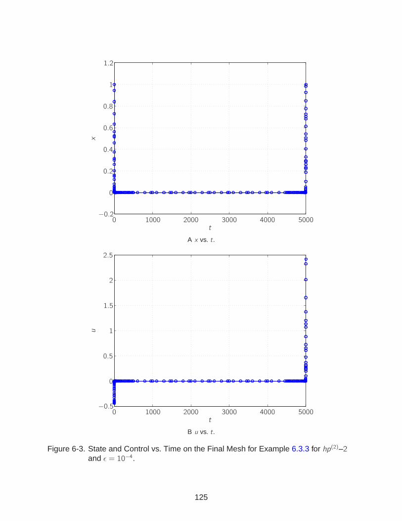
0
0
1x
t
−0.2
0.2
0.4
0.6
0.8
1.2
1000 2000 3000 4000 5000
A x vs. t.
0
0
1.5
2
2.5
−0.5
0.5
1
t
u
1000 2000 3000 4000 5000
B u vs. t.
Figure 6-3. State and Control vs. Time on the Final Mesh for Example 6.3.3 for hp(2)–2and ǫ = 10−4.
125
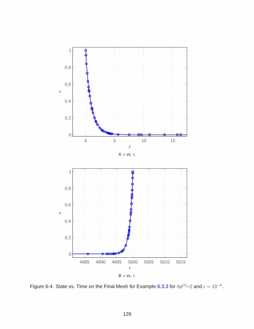
0
0
1
5 10 15
x
t
0.2
0.4
0.6
0.8
A x vs. t.
0
1
x
t
0.2
0.4
0.6
0.8
5000 5005 5010 50154985 4990 4995
B x vs. t.
Figure 6-4. State vs. Time on the Final Mesh for Example 6.3.3 for hp(2)–2 and ǫ = 10−4.
126

ǫ Strategy CPU Time (s) Colloc Pts Mesh Interval Mesh Iterations NLP Density10−2 p 13.11∗ 200∗ 1∗ 20∗ 50.12∗
hp(1) 0.84 45 7 6 12.74hp(2)–4 0.70 76 19 7 5.05hp(2)–3 0.42 68 22 8 5.02hp(2)–2 0.81 46 22 8 6.27h–2 0.38 54 27 8 5.25
10−4 p – – – – –hp(1) 1.41 70 10 9 9.05hp(2)–4 1.14 161 39 6 2.50hp(2)–3 1.21 151 46 8 2.42hp(2)–2 2.74 126 45 10 2.82h–2 1.12 200 100 9 1.48
10−6 p – – – – –hp(1) 3.73 110 12 9 7.78hp(2)–4 8.42 258 59 7 1.64hp(2)–3 5.69 217 55 8 1.93hp(2)–2 4.13 188 53 8 2.24h–2 107.91 1368 684 10 0.22
Table 6-10. Summary of Accuracy and Speed for Example 6.3.3 Using VariousCollocation Strategies and Accuracy Tolerances.
increased, the p–method becomes increasingly less capable of accurately approximating
the solution to this problem. For tf = 50, the p–method was able to approximate the
solution for ǫ = (10−2, 10−4) and for tf = 1000 the p–method was able to approximate the
solution for ǫ = 10−2. For tf = 5000, the p–method was unable to approximate solution to
the problem for any of the values of ǫ.
The h–2–method is much more insensitive than the p–method to the value of tf for
approximating the solution of this problem. Using a p–method, it is not possible to refine
the mesh specifically in regions where the error may be large. Because refinement
is necessary at the start and terminus of the solution, the h–2–method is much more
successful than the p–method in obtaining high-accuracy approximations to the solution
of this problem. However, because the h–2–method only uses low-order approximating
polynomials, when high accuracy is required, the number of approximating polynomials
is large. Even though the NLP is very sparse for the h–2–method, the size of the NLP
problem for high levels of accuracy results in a computationally inefficient NLP that
needs to be solved.
127
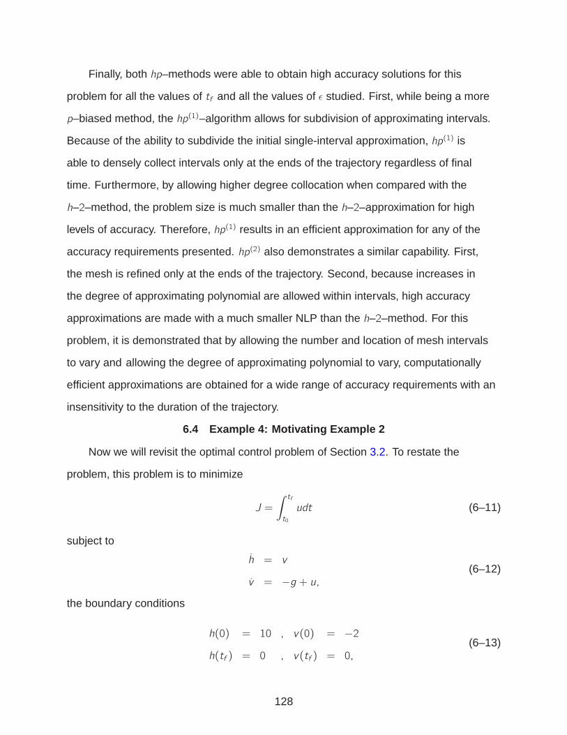
Finally, both hp–methods were able to obtain high accuracy solutions for this
problem for all the values of tf and all the values of ǫ studied. First, while being a more
p–biased method, the hp(1)–algorithm allows for subdivision of approximating intervals.
Because of the ability to subdivide the initial single-interval approximation, hp(1) is
able to densely collect intervals only at the ends of the trajectory regardless of final
time. Furthermore, by allowing higher degree collocation when compared with the
h–2–method, the problem size is much smaller than the h–2–approximation for high
levels of accuracy. Therefore, hp(1) results in an efficient approximation for any of the
accuracy requirements presented. hp(2) also demonstrates a similar capability. First,
the mesh is refined only at the ends of the trajectory. Second, because increases in
the degree of approximating polynomial are allowed within intervals, high accuracy
approximations are made with a much smaller NLP than the h–2–method. For this
problem, it is demonstrated that by allowing the number and location of mesh intervals
to vary and allowing the degree of approximating polynomial to vary, computationally
efficient approximations are obtained for a wide range of accuracy requirements with an
insensitivity to the duration of the trajectory.
6.4 Example 4: Motivating Example 2
Now we will revisit the optimal control problem of Section 3.2. To restate the
problem, this problem is to minimize
J =
∫ tf
t0
udt (6–11)
subject to
h = v
v = −g + u,(6–12)
the boundary conditions
h(0) = 10 , v(0) = −2
h(tf ) = 0 , v(tf ) = 0,(6–13)
128
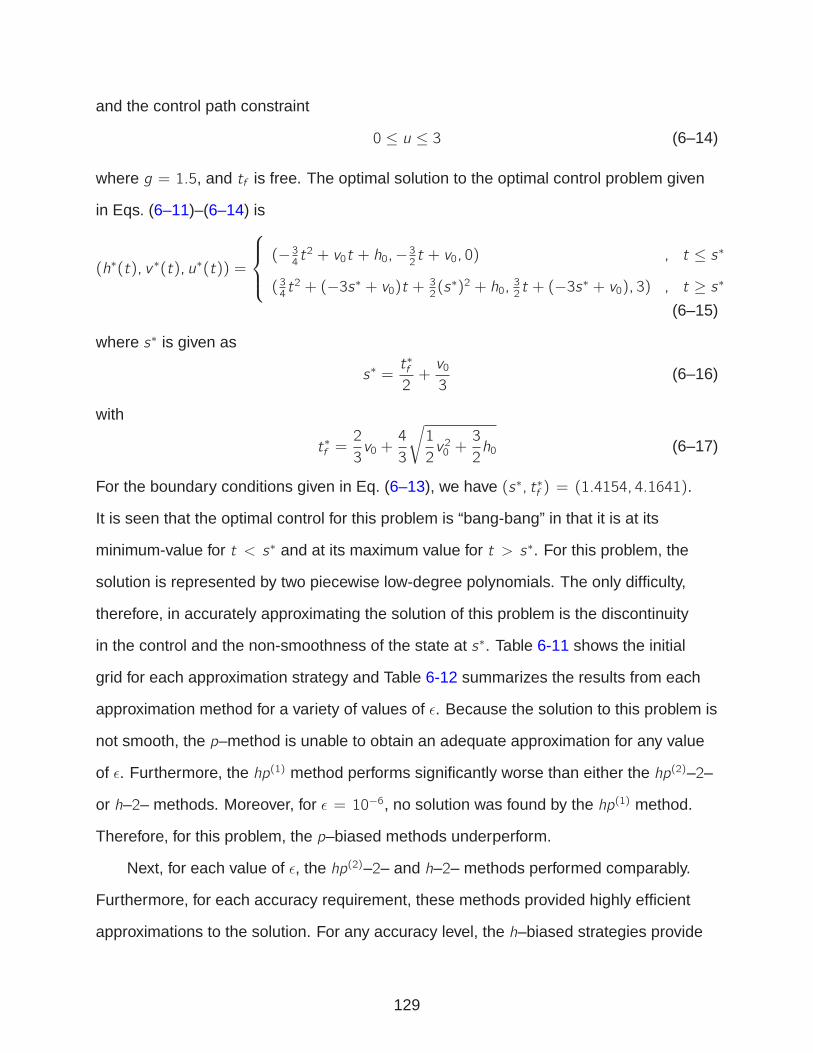
and the control path constraint
0 ≤ u ≤ 3 (6–14)
where g = 1.5, and tf is free. The optimal solution to the optimal control problem given
in Eqs. (6–11)–(6–14) is
(h∗(t), v ∗(t), u∗(t)) =
(−34t2 + v0t + h0,−32t + v0, 0) , t ≤ s∗
(34t2 + (−3s∗ + v0)t + 3
2(s∗)2 + h0,
32t + (−3s∗ + v0), 3) , t ≥ s∗
(6–15)
where s∗ is given as
s∗ =t∗f2+v0
3(6–16)
with
t∗f =2
3v0 +
4
3
√
1
2v 20 +
3
2h0 (6–17)
For the boundary conditions given in Eq. (6–13), we have (s∗, t∗f ) = (1.4154, 4.1641).
It is seen that the optimal control for this problem is “bang-bang” in that it is at its
minimum-value for t < s∗ and at its maximum value for t > s∗. For this problem, the
solution is represented by two piecewise low-degree polynomials. The only difficulty,
therefore, in accurately approximating the solution of this problem is the discontinuity
in the control and the non-smoothness of the state at s∗. Table 6-11 shows the initial
grid for each approximation strategy and Table 6-12 summarizes the results from each
approximation method for a variety of values of ǫ. Because the solution to this problem is
not smooth, the p–method is unable to obtain an adequate approximation for any value
of ǫ. Furthermore, the hp(1) method performs significantly worse than either the hp(2)–2–
or h–2– methods. Moreover, for ǫ = 10−6, no solution was found by the hp(1) method.
Therefore, for this problem, the p–biased methods underperform.
Next, for each value of ǫ, the hp(2)–2– and h–2– methods performed comparably.
Furthermore, for each accuracy requirement, these methods provided highly efficient
approximations to the solution. For any accuracy level, the h–biased strategies provide
129
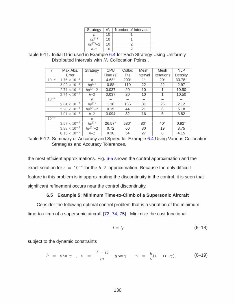
Strategy Nk Number of Intervalsp 10 1hp(1) 10 1hp(2)–2 10 2h–2 10 2
Table 6-11. Initial Grid used in Example 6.4 for Each Strategy Using UniformlyDistributed Intervals with Nk Collocation Points .
ǫ Max Abs. Strategy CPU Colloc Mesh Mesh NLPError Time (s) Pts Interval Iterations Density
10−2 1.76× 10⁻² p 4.68∗ 200∗ 1∗ 20∗ 33.78∗
3.02× 10−3 hp(1) 0.88 110 22 22 2.972.74× 10−2 hp(2)–2 0.037 20 10 1 10.502.74× 10−2 h–2 0.037 20 10 1 10.50
10−4 p – – – – –2.64× 10⁻³ hp(1) 1.18 155 31 25 2.125.20× 10−3 hp(2)–2 0.15 44 21 8 5.184.01× 10−3 h–2 0.094 32 16 5 6.82
10−6 p – – – – –3.57× 10⁻⁴ hp(1) 26.57∗ 580∗ 80∗ 40∗ 0.92∗
3.88× 10−5 hp(2)–2 0.72 60 30 19 3.758.15× 10−5 h–2 0.30 54 27 8 4.15
Table 6-12. Summary of Accuracy and Speed for Example 6.4 Using Various CollocationStrategies and Accuracy Tolerances.
the most efficient approximations. Fig. 6-5 shows the control approximation and the
exact solution for ǫ = 10−4 for the h–2–approximation. Because the only difficult
feature in this problem is in approximating the discontinuity in the control, it is seen that
significant refinement occurs near the control discontinuity.
6.5 Example 5: Minimum Time-to-Climb of a Supersonic Aircraft
Consider the following optimal control problem that is a variation of the minimum
time-to-climb of a supersonic aircraft [72, 74, 75] . Minimize the cost functional
J = tf (6–18)
subject to the dynamic constraints
h = v sin γ , v =T −Dm
− g sin γ , γ =g
v(n − cos γ), (6–19)
130

00
1.5
2
2
2.5
3
3
0.5
1
1 4 5
u
t
u∗(t)
u(t)
Figure 6-5. Control vs. Time on the Final Mesh for Example 6.4 Along with the ExactSolution.
the boundary conditions
h(0) = 0 , h(tf ) = 19995 m
v(0) = 129.31 m/s , v(tf ) = 295.09 m/s
γ(0) = 0 deg , γ(tf ) = 0 deg,
(6–20)
and the inequality path constraints
γ ≤ 45 deg, (6–21)
h ≥ 0 m,
where h is the altitude, v is the speed, γ is the flight path angle, g is the local acceleration
due to gravity, and n is the load factor (and is the control for this example). Further
131
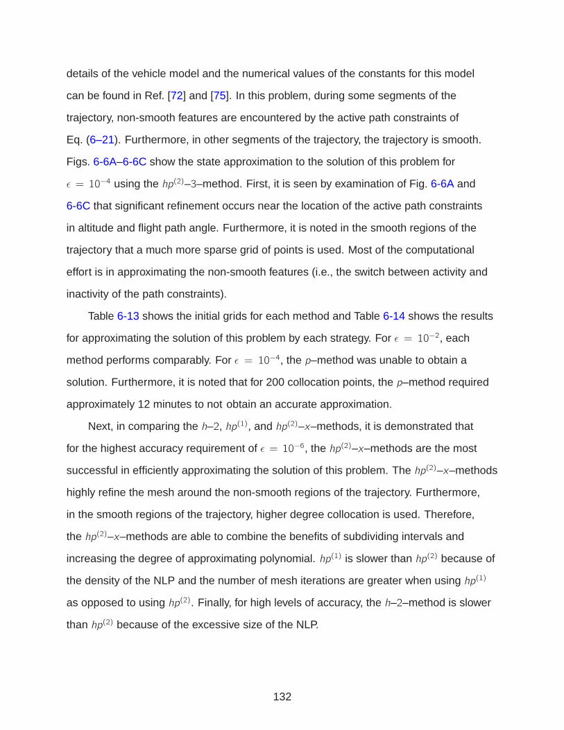
details of the vehicle model and the numerical values of the constants for this model
can be found in Ref. [72] and [75]. In this problem, during some segments of the
trajectory, non-smooth features are encountered by the active path constraints of
Eq. (6–21). Furthermore, in other segments of the trajectory, the trajectory is smooth.
Figs. 6-6A–6-6C show the state approximation to the solution of this problem for
ǫ = 10−4 using the hp(2)–3–method. First, it is seen by examination of Fig. 6-6A and
6-6C that significant refinement occurs near the location of the active path constraints
in altitude and flight path angle. Furthermore, it is noted in the smooth regions of the
trajectory that a much more sparse grid of points is used. Most of the computational
effort is in approximating the non-smooth features (i.e., the switch between activity and
inactivity of the path constraints).
Table 6-13 shows the initial grids for each method and Table 6-14 shows the results
for approximating the solution of this problem by each strategy. For ǫ = 10−2, each
method performs comparably. For ǫ = 10−4, the p–method was unable to obtain a
solution. Furthermore, it is noted that for 200 collocation points, the p–method required
approximately 12 minutes to not obtain an accurate approximation.
Next, in comparing the h–2, hp(1), and hp(2)–x–methods, it is demonstrated that
for the highest accuracy requirement of ǫ = 10−6, the hp(2)–x–methods are the most
successful in efficiently approximating the solution of this problem. The hp(2)–x–methods
highly refine the mesh around the non-smooth regions of the trajectory. Furthermore,
in the smooth regions of the trajectory, higher degree collocation is used. Therefore,
the hp(2)–x–methods are able to combine the benefits of subdividing intervals and
increasing the degree of approximating polynomial. hp(1) is slower than hp(2) because of
the density of the NLP and the number of mesh iterations are greater when using hp(1)
as opposed to using hp(2). Finally, for high levels of accuracy, the h–2–method is slower
than hp(2) because of the excessive size of the NLP.
132

00
5
10
10050 150 200
15
20
h(k
m)
t (sec)
400
A h vs. t.
0100
10050 150
200
200t (sec)
v(m
/s)
300
400
500
B v vs. t.
0
0−10
10
40
100
50
50 150 200
20
30
t (sec)
γ(d
eg)
C γ vs. t.
Figure 6-6. State vs. Time on the Final Mesh for Example 6.5 for hp(2)–3 and ǫ = 10−4.
Strategy Nk Number of Intervalsp 10 1hp(1) 10 1hp(2)–4 10 4hp(2)–3 10 3hp(2)–2 10 2h–2 10 2
Table 6-13. Initial Grid used in Example 6.5 for Each Strategy Using UniformlyDistributed Intervals with Nk Collocation Points.
133

ǫ Strategy CPU Time (s) Colloc Pts Mesh Interval Mesh Iterations NLP Density10−2 p 0.63 40 1 4 27.43
hp(1) 0.60 35 7 4 7.46hp(2)–4 0.37 48 12 2 5.01hp(2)–3 0.44 36 12 4 5.94hp(2)–2 0.25 24 12 3 7.73h–2 0.21 24 12 2 7.73
10−4 p 707.67∗ 200∗ 1∗ 20∗ 25.51∗
hp(1) 4.20 125 15 9 4.30hp(2)–4 1.74 86 21 6 2.89hp(2)–3 0.28 69 20 6 3.42hp(2)–2 0.95 78 29 6 2.85h–2 0.87 110 55 4 1.79
10−6 p – – – – –hp(1) 69.70 245 17 18 7.56hp(2)–4 14.75 217 50 8 1.20hp(2)–3 19.84 241 62 10 1.06hp(2)–2 19.09 359 86 7 0.73h–2 115.01 934 467 6 0.21
Table 6-14. Summary of Accuracy and Speed for Example 6.5 Using Various CollocationStrategies and Accuracy Tolerances.
6.6 Discussion of Results
The results of the five examples demonstrate some of the key characteristics of
approximating problems by hp–mesh refinement algorithm 1 and hp–mesh refinement
algorithm 2. In Example 6.1, the solution is smooth and the p and hp(1) methods perform
exactly the same. As expected, the most efficient approximation to this problem is by
a p–method. Furthermore, as expected, for tight accuracy tolerances, the h–2–method
is computationally inefficient. hp–mesh refinement algorithm 2 had comparable CPU
times to the p–method for all values of ǫ. By a relatively modest increase in degree of
approximation coupled with the increased sparsity of the approximation in hp–mesh
refinement algorithm 2, efficient approximations to the solution of the first example
problem were obtained.
In Example 2, the solution to the problem appears to be smooth, but is more
complicated than Example 6.1. For this example, as the accuracy tolerance was
tightened, the p–method provided the best approximation. Furthermore, as the
accuracy tolerance was tightened, the h–2–method became computationally inefficient.
134
Surprisingly for this example, hp–mesh refinement algorithm 1 was less efficient than
hp–mesh refinement algorithm 2. The inefficiency of hp–mesh refinement algorithm 1
is largely due to the excessive number of mesh iterations required to find a solution.
Furthermore, while the p–method provides the most efficient solution approximation
to this problem for a high accuracy requirement, it is interesting to note that hp–mesh
refinement algorithm 2 does not significantly underperform. While a single high-degree
approximating interval provides the most efficient approximation to the solution of this
problem, it is interesting to note that many intervals of moderate degree also accurately
and efficiently approximate the solution of this problem. The combined affects of using
moderate degree intervals and a sparse NLP provides comparable efficiency to the
p–method.
Example 6.3 studies a problem for three different values of tf where the chosen
values of tf change the inherent timescale of the problem. In this problem, a p–method
has an increasingly difficult time finding a suitable approximation as the final time is
increased. Furthermore, for very high accuracy requirements, the h–2-method is again
seen to provide inefficient results. Finally, both hp–algorithms performed well for any
value of tf . The combined ability to refine the location of mesh intervals and the use of
a variable degree polynomial in each interval make the hp–algorithms successful for
approximating the solution of this problem.
The solution structure to Example 6.4 is significantly different from the previous
three examples. The solution to this problem is represented by two piecewise low-degree
polynomials. Because the control is discontinuous the connection between these two
piecewise polynomials is non-smooth. In this problem, a p–method was unable to find
an accurate approximation for any value of ǫ because of the non-smooth nature of the
solution to this problem. hp–mesh refinement algorithm 1 performed significantly worse
when compared with hp–mesh refinement algorithm 2 or the h–2–method and was not
135

able to find a solution for the tightest accuracy tolerance. For any value of ǫ, hp–mesh
refinement algorithm 2 or the h–2–method performed well.
The final example is a modified version of the minimum time-to-climb of a
supersonic aircraft. This example has non-smooth regions of the trajectory and smooth
regions of the trajectory. Because of the non-smoothness that exists, the p–method
was not able to find approximations for tight accuracy tolerances. Furthermore,
hp–mesh refinement algorithm 2 outperformed hp–mesh refinement algorithm 1 and
the h–2–method. hp–mesh refinement algorithm 2 more successfully simultaneously
handled non-smooth and smooth features than hp–mesh refinement algorithm 1 or the
h–method.
In summary, the method that will best approximates the solution of an optimal
control problem is problem dependent. If a problem is simple and smooth, a p–method
performs the best. In any other case, a p–method does not perform well. hp–mesh
refinement algorithm 1 improves upon the robustness of a strictly p–method for
approximating the solution to problems that may be non-smooth. For problems with
nonsmooth features, hp–mesh refinement algorithm 1 requires more computational time
than hp–mesh refinement algorithm 2 or the h–2–method.
By an h–method, low-accuracy solutions can be obtained to a wide variety of
problems in a computationally efficient manner. On the other hand, high-accuracy
solutions require a tremendous computational burden because of the large problem
size of the h–methods. hp–mesh refinement algorithm 2 performed much better.
Furthermore, for every example problem of this chapter, hp–mesh refinement algorithm
2 performed either better than the other methods or was comparable to the best
method for each problem (i.e., p for problems with simple smooth solutions or h for
problems with nonsmooth solutions with no high-order behaviors). It is demonstrated by
hp–mesh refinement algorithm 2 that high accuracy solutions to problems do not require
high-degree polynomials. The highest degree polynomial used by hp–mesh refinement
136

algorithm 2 in any of the examples is eighth order. If exponential convergence is
expected in a particular interval, a high-degree polynomial approximation should
not be required. Furthermore, because low and mid-degree polynomials are used,
hp–mesh refinement algorithm 2 results in an NLP that is sparse. Moreover, by
specifically refining only parts of an approximation with the largest errors, the distribution
of the mesh focuses only on those locations that need more mesh intervals or
mid-degree approximating polynomials. hp–mesh refinement algorithm 2 demonstrates
significant robustness irregardless of accuracy requirement or problem type on the
examples in this Chapter. As a starting point, hp–mesh refinement algorithm 2 utilizes
low-degree polynomials that ensure a sparse NLP. Refinement of the mesh occurs in
regions of large error, and mid-degree polynomials are used on intervals with smooth
solutions. Therefore, the computational efficiency of an h–method is combined with the
high-accuracy of a p–method.
137
CHAPTER 7AEROASSISTED ORBITAL INCLINATION CHANGE MANEUVER
In this Chapter, an aeroassisted orbital inclination change maneuver for a small
maneuverable spacecraft in low-Earth orbit (LEO) is studied. It is known that using
atmospheric force (namely, lift and drag) may significantly reduce the amount of fuel
required to change the inclination of the vehicle as compared to an all-propulsive
maneuver [76]. The survey papers of Ref. [77] and [78] summarize early work on
aeroassisted orbital transfers. Ref. [79] studied multiple-pass aeroassisted gliding
maneuvers with a large inclination change of a large spacecraft between geostationary
orbit (GEO) and LEO. A key result of Ref. [79] is that the aeroassisted maneuver was
much more fuel efficient than an all-propulsive maneuver. Furthermore, in Ref. [79],
it was demonstrated for highly constrained heating rates on the vehicle that the fuel
required to accomplish the maneuver decreased as the number of atmospheric passes
increased.
While previous research on aeroassisted orbital inclination change maneuvers has
been for large spacecraft, in this research, we consider a LEO to LEO aeroassisted
orbital transfer of a small maneuverable spacecraft. The aeroassisted maneuver is
compared against all-propulsive maneuvers. The multiple-pass aeroassisted glide
maneuvers are analyzed as functions of the number of atmospheric passes, the required
inclination change, and the maximum allowable heating rate on the vehicle. The results
of this Chapter are similar to the results found in Ref. [80].
138
7.1 Equations of Motion
The equations of motion over a spherical non-rotating Earth are given in spherical
coordinates as [19, 79, 81]
r = v sin γ,
θ =v cos γ cosψ
r cosφ,
φ =v cos γ sinψ
r,
v = −Dm
− µ
r 2sin γ,
γ =1
v
[
−L cos σm
−(
µ
r 2− v
2
r
)
cos γ
]
,
ψ =1
v
[
− L sinσm cos γ
− v2
rcos γ cosψ tanφ
]
,
(7–1)
where r is the geocentric radius, θ is the longitude, φ is the latitude, v is the speed, γ is
the flight path angle, ψ is the heading angle, D is the drag force, L is the lift force, µ is
the Earth gravitational parameter, and σ is the bank angle. Next, it is noted that drag and
lift are modeled, respectively, as [19]
D =1
2ρv 2ACD (7–2)
L =1
2ρv 2ACL (7–3)
where ρ is the atmospheric density, A is the vehicle reference area, CD is the coefficient
of drag, and CL is the coefficient of lift. The atmospheric density is modeled as an
exponential of the form
ρ = ρ0 exp(−βh), (7–4)
where ρ0 is the atmospheric density at sea level, β is the inverse of density scale height,
and h = r − Re is the altitude where Re is the radius of the Earth. The aerodynamic
139
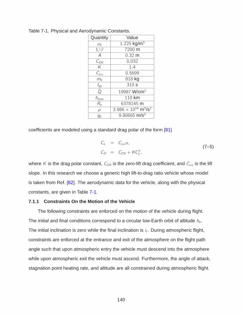
Table 7-1. Physical and Aerodynamic Constants.Quantity Value
ρ0 1.225 kg/m3
1/β 7200 mA 0.32 mCD0 0.032
K 1.4
CLα 0.5699
m0 818 kgIsp 310 s˙Q 19987W/cm2
hatm 110 kmRe 6378145 mµ 3.986× 10¹⁴ m3/s2
g0 9.80665 m/s2
coefficients are modeled using a standard drag polar of the form [81]
CL = CLαα,
CD = CD0 + KC2L ,
(7–5)
where K is the drag polar constant, CD0 is the zero-lift drag coefficient, and CLα is the lift
slope. In this research we choose a generic high lift-to-drag ratio vehicle whose model
is taken from Ref. [82]. The aerodynamic data for the vehicle, along with the physical
constants, are given in Table 7-1.
7.1.1 Constraints On the Motion of the Vehicle
The following constraints are enforced on the motion of the vehicle during flight.
The initial and final conditions correspond to a circular low-Earth orbit of altitude h0.
The initial inclination is zero while the final inclination is if . During atmospheric flight,
constraints are enforced at the entrance and exit of the atmosphere on the flight path
angle such that upon atmospheric entry the vehicle must descend into the atmosphere
while upon atmospheric exit the vehicle must ascend. Furthermore, the angle of attack,
stagnation point heating rate, and altitude are all constrained during atmospheric flight.
140
7.1.1.1 Initial and final conditions
The initial conditions for this study correspond to a circular equatorial orbit of
altitude h0. The initial orbital conditions for this problem are given in terms of orbital
elements [83] as
a(t0) = Re + h0 , e(t0) = 0
i(t0) = 0 , Ω(t0) = 0
ω(t0) = 0 , ν(t0) = 0,
(7–6)
where a is the semi-major axis, i is the inclination, ω is the argument of perigee, e is the
eccentricity, Ω is the longitude of ascending node, and ν is the true anomaly. The values
for Ω(t0),ω(t0), and ν(t0) are arbitrarily set to zero. Furthermore, the final conditions for
this problem are for a circular orbit of altitude hf = h0 with an inclination if and are given
as
a(tf ) = Re + hf , e(tf ) = 0 , i(tf ) = if , (7–7)
Because the final orbit is circular and the location of the spacecraft in the terminal orbit
is not constrained, ω(tf ) is undefined and ν(tf ) and Ω(tf ) are free.
7.1.1.2 Interior point constraints
Along with the initial and final conditions on the vehicle, the following interior-point
constraints are enforced at every atmospheric entrance:
r (tatm0 ) = hatm + Re,
γ (tatm0 ) ≤ 0,
(7–8)
where tatm0 is the beginning of any atmospheric flight segment and hatm is the edge
of the sensible atmosphere. These constraints ensure that at the entrance of any
atmospheric flight segment the vehicle is descending into the atmosphere. Furthermore,
at the exit of any atmospheric flight segment, the following constraints are imposed such
141
that the vehicle is ascending upon atmospheric exit:
r (tatmf ) = hatm + Re,
γ (tatmf ) ≥ 0,
(7–9)
where t(atm)f is the time at the end of any atmospheric flight segment.
7.1.1.3 Vehicle path constraints
The following inequality path constraints are enforced during atmospheric flight. The
angle of attack is constrained as
0 ≤ α ≤ αmax. (7–10)
Next, the stagnation point heating rate is constrained. Using the Chapman equation [84],
the stagnation point heating rate, Q, is given as
Q = ˙Q(ρ/ρ0)0.5(v/vc)
3.15, (7–11)
where vc =√
µ/Re . Therefore, during atmospheric flight, the following constraint on
heating rate is imposed:
0 ≤ Q ≤ Qmax. (7–12)
Finally, during atmospheric flight, the altitude is constrained as:
0 ≤ h ≤ hatm (7–13)
or, alternatively,
Re ≤ r ≤ hatm + Re. (7–14)
7.1.2 Trajectory Event Sequence
The trajectory event sequence for a maneuver with n atmospheric passes is now
described. From the initial conditions of Eq. (7–6), a deorbit velocity impulse, ∆V1, is
applied to send the vehicle into the atmosphere. The vehicle then glides in and out of
the atmosphere n times. Upon the final atmospheric exit, a boost velocity impulse, ∆V2,
142
is applied to give the vehicle enough energy to reach the final orbit condition. Upon
reaching the final orbital altitude, a final recircularization velocity impulse, ∆V3 is applied
to recircularize the orbit. The trajectory event sequence is now described in detail (see
Figs. 7-1A–7-1C):
(i) Event: ∆V1 is applied to the initial orbital conditions in Eq. (7–6);
(ii) Phase: an exo-atmospheric glide that terminates at the edge of the sensibleatmosphere (hatm);
(iii) Phase: an atmospheric glide that terminates at the edge of the sensible atmosphere(hatm);
The following two phases are then repeated for the remaining n − 1 atmospheric passes:
(iv) Phase: an exo-atmospheric glide that terminates at the edge of the sensibleatmosphere (hatm);
(v) Phase: an atmospheric glide that terminates at the edge of the sensible atmosphere(hatm);
Upon the final atmospheric exit, the following events and phase occur:
(vii) Event: ∆V2 is applied at the maximum altitude of the sensible atmosphere;
(viii) Phase: an exo-atmospheric glide that terminates at the final orbital altitude;
(ix) Event: ∆V3 is applied at the final orbital altitude to re-circularize the orbit.
7.1.3 Performance Index
The cost functional for the multiple-pass aeroglide maneuver is to minimize the fuel
consumed during the maneuver. This corresponds to minimizing the negative of the final
mass, i.e.,
J = −m(tf ). (7–15)
Assuming impulsive thrust, ∆V ≡ ‖∆V‖, the mass after each impulse is then computed
from the Goddard rocket equation as
m+ = m− exp(−∆Vg0Isp
), (7–16)
143

A Deorbit and First Atmospheric Flight Segment.
B Intermediate Exo-Atmospheric and AtmosphericFlight Segments.
C Final Exo-Atmospheric Flight Segment.
Figure 7-1. Schematic of Trajectory Design for Aeroassisted Orbital Transfer Problem.
144

where m− and m+ are the values of the mass immediately before and after application
of the impulse. Therefore, the final mass after three velocity impulses is given as
m(tf ) = m(t0)exp(−(∆V1 + ∆V2 + ∆V3))
g0Isp. (7–17)
7.2 Re-Formulation of Problem
The manner in which the multiple-pass aeroassisted orbital transfer is solved
differs slightly from the formulation given in Section 7.1. Instead of using α and σ as the
controls, the quantities u1 and u2 are used as controls, where u1 and u2 are defined as
u1 = −CL sinσ,
u2 = −CL cos σ.(7–18)
In terms of u1 and u2, CL and σ are given as
CL =
√
u21 + u22 (7–19)
σ = tan−1(u1/u2). (7–20)
It is noted that u1 and u2 are used instead of the more obvious choices of coefficient
of lift and bank angle because u1 and u2 avoid the wrapping problem that arises
when using angles as controls [19]. In terms of u1 and u2, the differential equations
of Eq. (7–1) are given as
r = v sin γ,
θ =v cos γ cosψ
r cosφ,
φ =v cos γ sinψ
r,
v = −ρv2ACD
2m− µ
r 2sin γ,
γ =1
v
[
−ρv2A
2mu2 −
(
µ
r 2− v
2
r
)
cos γ
]
,
ψ =1
v
[
− ρv 2A
2m cos γu1 −
v 2
rcos γ cosψ tanφ
]
.
(7–21)
145
Next, because the coefficient of lift is linear in α, the constraint on α in Eq. (7–10) is
equivalently written as
0 ≤ CL ≤ CL, (7–22)
where CL denotes the maximum allowable value of CL. Therefore, the controls u1 and u2
are constrained as
− CL ≤ (u1, u2) ≤ CL, (7–23)
0 ≤ u21 + u22 ≤ C 2L . (7–24)
In this study the maximum allowable angle of attack is αmax ≈ 40 deg which corresponds
to CL = 0.4.
Next, the heating rate constraint of Eq. (7–11) is rewritten to be better behaved
computationally. Specifically, instead of constraining Q, we constrain the natural
logarithm of Q, log Q, as
−∞ ≤ log Q ≤ log Qmax, (7–25)
Using the above formulations, the optimal control problem corresponding to the
aeroassisted orbital transfer problem was solved in canonical units where length is
measured in Earth radii, time is measured in units of√
R3e /µ, speed is measured in units
of√
µ/Re , and mass is measured in units of m0, the initial mass of the vehicle. This
system of units is used because it is well-scaled.
7.3 Optimal Control Problem
The optimal control problem corresponding to the minimum-fuel aeroassisted orbital
transfer problem is now stated. Minimize the cost functional of Eq. (7–15) subject to the
dynamic constraints of Eqs. (7–21), the path constraints of Eqs. (7–14), (7–23), (7–24),
and (7–25), and the interior point constraints of Eqs. (7–8) and (7–9). The optimal
control problem is solved using the hp–mesh refinement algorithm of Ref. [67] which is
implemented in the software GPOPS [26, 67] and uses the NLP solver SNOPT [11, 68].
146

All NLP derivatives were computed using the Matlab automatic differentiator INTLAB
[85].
7.4 All-Propulsive Inclination Change Maneuvers
The following two all-propulsive transfers are studied in order to compared with the
aeroassisted orbital inclination change maneuver: (1) a single impulse direct change in
inclination via rotation of the initial velocity and (2) a two impulse bi-parabolic transfer.
Figs. 7-2A and 7-2B show the single impulse and bi-parabolic transfers, respectively. It
is seen that the single impulse transfer rotates the orbital velocity vector by an angle ∆i .
Next, the first impulse of the bi-parabolic transfer sends the orbit to an orbit of infinite
radius where the change in inclination is free. Upon return to the initial orbit, a second
impulse is applied to recircularize the orbit. For initial and terminal circular orbits of the
same size but with different inclinations, the direct impulse and total bi-parabolic impulse
required to change inclination by an amount ∆i are given, respectively, as [86]
∆V = 2v0 sin∆i2,
∆V = 2(√2− 1)v0,
(7–26)
where v0 is the initial orbital speed. By inspection, it is seen that the bi-parabolic
transfer is more efficient for ∆i > 49 degrees. Therefore, when comparing the optimal
aeroassisted orbital transfer fuel consumption with all-propulsive maneuvers, the
aeroassisted orbital transfer fuel consumption is compared with the single impulse
maneuver when ∆i ≤ 49 deg and is compared with the bi-parabolic transfer when
∆i > 49 deg.
7.5 Results
The multiple-pass aeroassisted orbital transfer optimal control problem summarized
in Section 7.3 was solved for n = (1, 2, 3, 4) atmospheric passes. Furthermore,
for each value of n, a change of inclination of if = (20, 40, 60, 80) deg subject to
Qmax = (400, 800, 1200,∞) W/cm2 is studied.
147

A Single Impulse Transfer.
B Bi-parabolic Transfer.
Figure 7-2. Schematic of All-Propulsive Single Impulse and Bi-Parabolic Transfers.
148
7.5.1 Unconstrained Heating Rate
The cost of the multiple-pass aeroassisted orbital transfer is first shown with no
constraint on heating rate. Fig. 7-3A shows the minimum impulse, ∆Vmin, required
to change the inclination of the orbital vehicle for one, two, three and four pass
aeroassisted maneuvers and the all-propulsive maneuvers. First, it is interesting to
note that because the bi-parabolic maneuver has a constant cost, the cost for the
60 deg and 80 deg all-propulsive inclination changes are equivalent. Next, it is seen
for very small inclination change (i.e., 1 deg), there is virtually no difference in cost
between aeroassisted maneuvers and all-propulsive maneuvers. For if = (20, 40, 60, 80)
deg, it is seen that the aeroassisted maneuvers can dramatically reduce costs when
compared with the all-propulsive maneuvers. The cost for a required inclination change
is insensitive to the number of atmospheric passes. For n = (1, 2, 3, 4), the costs are
nearly identical for any given value if . This is seen in Fig. 7-3B. In this figure, the final
mass fraction after completion of the aeroassisted maneuver is shown. It is seen that
for the range of inclination changes, a large fraction of the final mass is retained for the
vehicle after the maneuver is completed. For a 20 degree inclination change, more than
60% of the final mass is retained. Furthermore, for an 80 degree inclination change
maneuver, approximately 30% of the final mass is retained after completion of the
maneuver.
Next, Figs. 7-4A–7-4D show the impulses for ∆V1, ∆V2, and ∆V3 along with the total
loss of velocity from drag, ∆VD . First, it is noted that the deorbit and recircularization
impulses, ∆V1 and ∆V3, are very small. Regardless of the amount of inclination change
that is desired, these impulses are much smaller than the boost impulse, ∆V2. When
comparing Figs. 7-4B and 7-4D, it is seen that the majority of the boost impulse is used
to recover velocity lost due to atmospheric drag. Therefore, as expected, the cost of the
aeroassisted maneuver is largely due to recovering energy lost due to drag.
149
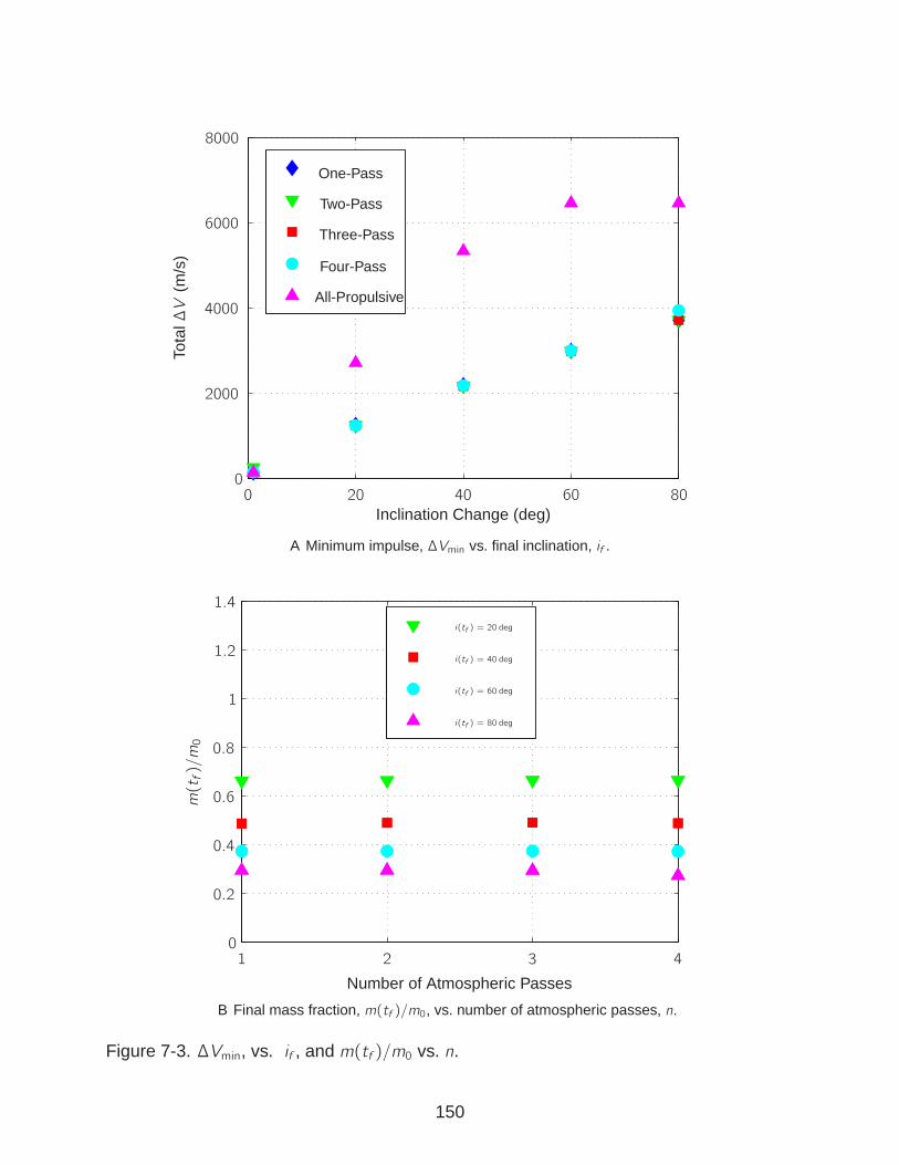
Tota
l∆V
(m/s
)
Inclination Change (deg)
One-Pass
Two-Pass
Three-Pass
Four-Pass
All-Propulsive
00
2000
4000
40 60 8020
6000
8000
max
A Minimum impulse, ∆Vmin vs. final inclination, if .
1.2
0
1
1 32 4
0.8
0.6
0.4
0.2
i(tf ) = 20 deg
i(tf ) = 40 deg
i(tf ) = 60 deg
i(tf ) = 80 deg
Number of Atmospheric Passes
m(tf)/m0
1.4
B Final mass fraction, m(tf )/m0, vs. number of atmospheric passes, n.
Figure 7-3. ∆Vmin, vs. if , and m(tf )/m0 vs. n.
150

1 328
32
34
36
38
30
2 4
i(tf ) = 20 deg
i(tf ) = 40 deg
i(tf ) = 60 deg
i(tf ) = 80 deg
Number of Atmospheric Passes
∆V1
(m/s
)
A ∆V1, vs. n.
1 31000
2000
3000
2 4
4000
5000
6000i(tf ) = 20 deg
i(tf ) = 40 deg
i(tf ) = 60 deg
i(tf ) = 80 deg
Number of Atmospheric Passes
∆V2
(m/s
)
B ∆V2, vs. n.
01 3
30
50
2 4
10
40
60
20
i(tf ) = 20 deg
i(tf ) = 40 deg
i(tf ) = 60 deg
i(tf ) = 80 deg
Number of Atmospheric Passes
∆V3
(m/s
)
C ∆V3, vs. n.
1 31000
2000
3000
2 4
4000
5000
6000i(tf ) = 20 deg
i(tf ) = 40 deg
i(tf ) = 60 deg
i(tf ) = 80 deg
Number of Atmospheric Passes
∆VD
(m/s
)
D ∆VD , vs. n.
Figure 7-4. ∆V1, ∆V2, ∆V3, and ∆VD Impulses vs. n.
Figs. 7-5A shows the total inclination change achieved by atmospheric forces as a
function of number of passes and required inclination change. It is seen that for each
required inclination change, the majority of the inclination change is performed by the
atmosphere. It is interesting to note for if = 80 deg that the four-pass maneuver has
less inclination change from the atmosphere as compared with the one, two or three
pass maneuvers. Nevertheless, the cost of the if = 80 deg maneuver is nearly the same
as the cost of the one, two or three pass maneuvers. Next, Fig. 7-5B shows the total
transfer time for n = (1, 2, 3, 4) for if = (20, 40, 60, 80). As expected, the total transfer
151
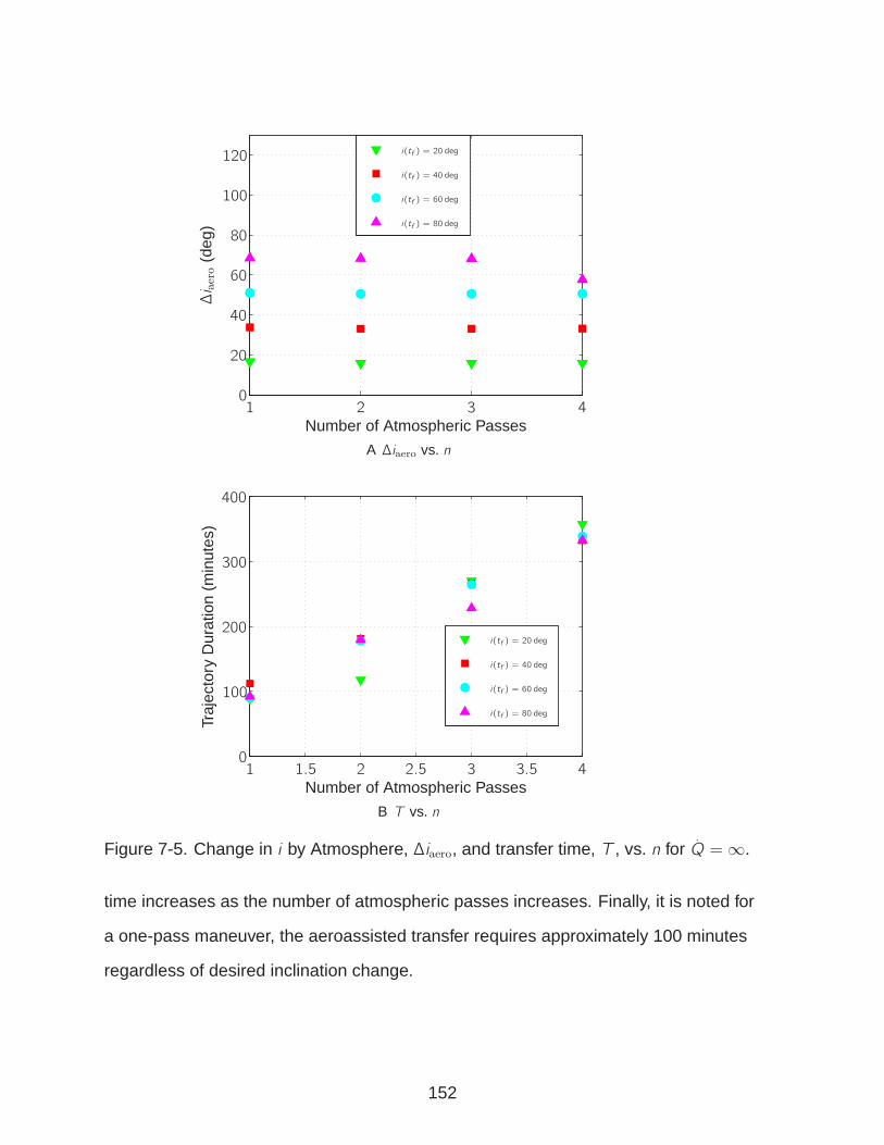
01 32 4
40
60
80
100
120
20
i(tf ) = 20 deg
i(tf ) = 40 deg
i(tf ) = 60 deg
i(tf ) = 80 deg
Number of Atmospheric Passes
∆i aero
(deg
)
A ∆iaero vs. n
01 3 3.51.5 2.52 4
200
400
100
300
i(tf ) = 20 deg
i(tf ) = 40 deg
i(tf ) = 60 deg
i(tf ) = 80 deg
Number of Atmospheric Passes
Traj
ecto
ryD
urat
ion
(min
utes
)
B T vs. n
Figure 7-5. Change in i by Atmosphere, ∆iaero, and transfer time, T , vs. n for Q =∞.
time increases as the number of atmospheric passes increases. Finally, it is noted for
a one-pass maneuver, the aeroassisted transfer requires approximately 100 minutes
regardless of desired inclination change.
152
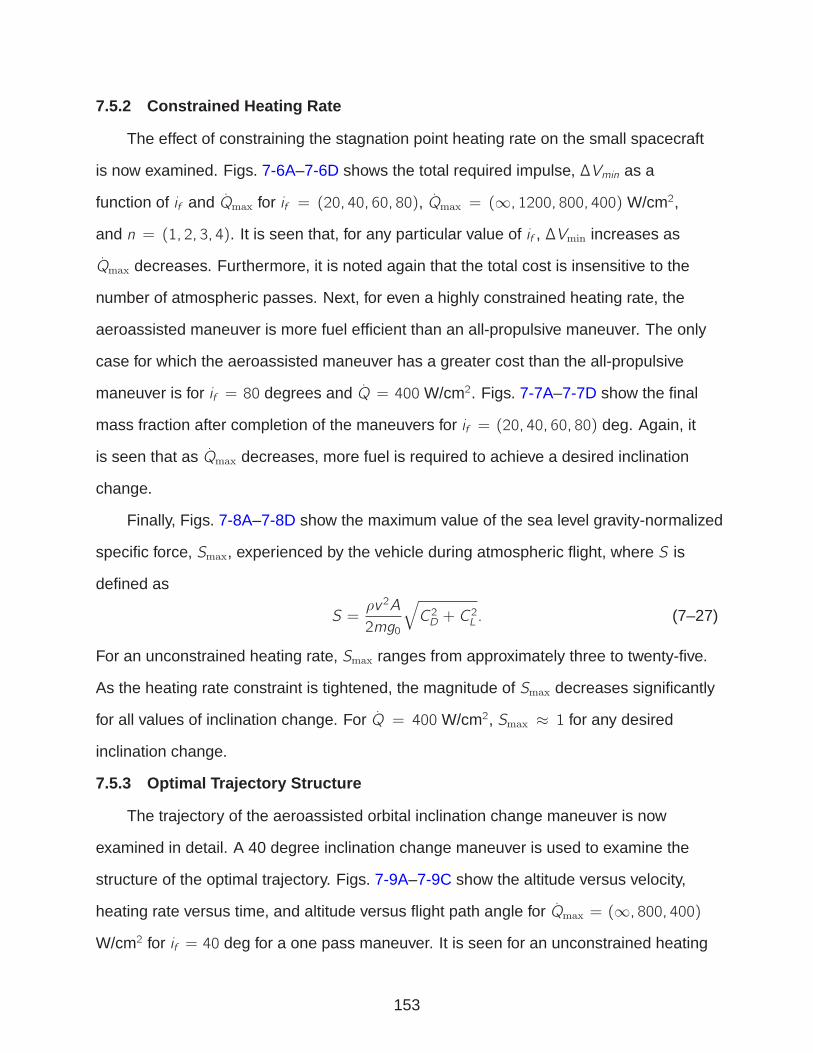
7.5.2 Constrained Heating Rate
The effect of constraining the stagnation point heating rate on the small spacecraft
is now examined. Figs. 7-6A–7-6D shows the total required impulse, ∆Vmin as a
function of if and Qmax for if = (20, 40, 60, 80), Qmax = (∞, 1200, 800, 400) W/cm2,
and n = (1, 2, 3, 4). It is seen that, for any particular value of if , ∆Vmin increases as
Qmax decreases. Furthermore, it is noted again that the total cost is insensitive to the
number of atmospheric passes. Next, for even a highly constrained heating rate, the
aeroassisted maneuver is more fuel efficient than an all-propulsive maneuver. The only
case for which the aeroassisted maneuver has a greater cost than the all-propulsive
maneuver is for if = 80 degrees and Q = 400W/cm2. Figs. 7-7A–7-7D show the final
mass fraction after completion of the maneuvers for if = (20, 40, 60, 80) deg. Again, it
is seen that as Qmax decreases, more fuel is required to achieve a desired inclination
change.
Finally, Figs. 7-8A–7-8D show the maximum value of the sea level gravity-normalized
specific force, Smax, experienced by the vehicle during atmospheric flight, where S is
defined as
S =ρv 2A
2mg0
√
C 2D + C2L . (7–27)
For an unconstrained heating rate, Smax ranges from approximately three to twenty-five.
As the heating rate constraint is tightened, the magnitude of Smax decreases significantly
for all values of inclination change. For Q = 400W/cm2, Smax ≈ 1 for any desired
inclination change.
7.5.3 Optimal Trajectory Structure
The trajectory of the aeroassisted orbital inclination change maneuver is now
examined in detail. A 40 degree inclination change maneuver is used to examine the
structure of the optimal trajectory. Figs. 7-9A–7-9C show the altitude versus velocity,
heating rate versus time, and altitude versus flight path angle for Qmax = (∞, 800, 400)
W/cm2 for if = 40 deg for a one pass maneuver. It is seen for an unconstrained heating
153

All-Propulsive
1 31000
2000
3000
2 4
4000
5000
Number of Atmospheric Passes
∆Vmin
(m/s
)
Qmax =∞ (W/cm2)
Qmax = 1200 (W/cm2)
Qmax = 800 (W/cm2)
Qmax = 400 (W/cm2)
A ∆Vmin vs. n for if = 20 deg.
All-Propulsive
1 32000
2 4
4000
6000
8000
Number of Atmospheric Passes
∆Vmin
(m/s
)
10000Qmax =∞ (W/cm2)
Qmax = 1200 (W/cm2)
Qmax = 800 (W/cm2)
Qmax = 400 (W/cm2)
B ∆Vmin vs. n for if = 40 deg.
All-Propulsive
1 3
12000
2 4
4000
6000
8000
Number of Atmospheric Passes
∆Vmin
(m/s
) 10000
Qmax =∞ (W/cm2)
Qmax = 1200 (W/cm2)
Qmax = 800 (W/cm2)
Qmax = 400 (W/cm2)
C ∆Vmin vs. n for if = 60 deg.
All-Propulsive
1 3
12000
14000
2 4
4000
6000
8000
Number of Atmospheric Passes
∆Vmin
(m/s
)
10000
Qmax =∞ (W/cm2)
Qmax = 1200 (W/cm2)
Qmax = 800 (W/cm2)
Qmax = 400 (W/cm2)
D ∆Vmin vs. n for if = 80 deg.
Figure 7-6. ∆Vmin, vs. n for Various Max Heating Rates and Final Inclinations.
rate, the vehicle dives deeply into the atmosphere once and then ascends back out of
the atmosphere. For the cases of Qmax = (800, 400)W/cm2, it is seen that the vehicle
descends until reaching the maximum value of the heating rate constraint. The vehicle
then glides at the maximum value of the heating rate constraint for a short duration
before re-ascending to near the edge of the atmosphere. The vehicle then descends
again to reach the heating rate constraint before reascending out of the atmosphere.
Therefore, for a one-pass maneuver with an active constraint on the heating rate, the
trajectory essentially becomes a two-pass maneuver. Figs. 7-10A and 7-10B show the
154

All-Propulsive
0
1
1 3
0.5
1.5
2 4Number of Atmospheric Passes
m(tf)/m0
Qmax =∞ (W/cm2)
Qmax = 1200 (W/cm2)
Qmax = 800 (W/cm2)
Qmax = 400 (W/cm2)
A m(tf )/m0 vs. n for if = 20 deg.
1.2
All-Propulsive
0
1
1 32 4
0.8
0.6
0.4
0.2
Number of Atmospheric Passes
m(tf)/m0
1.4Qmax =∞ (W/cm2)
Qmax = 1200 (W/cm2)
Qmax = 800 (W/cm2)
Qmax = 400 (W/cm2)
B m(tf )/m0 vs. n for if = 40 deg.
All-Propulsive
0
1
1 32 4
0.8
0.6
0.4
0.2
Number of Atmospheric Passes
m(tf)/m0
Qmax =∞ (W/cm2)
Qmax = 1200 (W/cm2)
Qmax = 800 (W/cm2)
Qmax = 400 (W/cm2)
C m(tf )/m0 vs. n for if = 60 deg.
All-Propulsive
0
1
1 32 4
0.8
0.6
0.4
0.2
Number of Atmospheric Passes
m(tf)/m0
Qmax =∞ (W/cm2)
Qmax = 1200 (W/cm2)
Qmax = 800 (W/cm2)
Qmax = 400 (W/cm2)
D m(tf )/m0 vs. n for if = 80 deg.
Figure 7-7. m(tf )/m0, vs. n for Various Qmax, and if = (20, 40, 60, 80) deg.
angle of attack and bank angle for the vehicle for the one-pass maneuver. It is seen that
for each value of heating rate constraint, the vehicle enters and exits the atmosphere
with a near maximum value of angle of attack of approximately 40 deg. Furthermore, it
is seen that the vehicle enters at a nearly 90 deg bank angle, rotates 180 degrees, and
exits at a nearly -90 deg bank angle.
Figs. 7-11A–7-11D show the altitude versus velocity for one, two, three and four
pass maneuvers for if = 40 degrees and Qmax = 400W/cm2. It is interesting to note that
the profiles are nearly identical regardless of number of passes. For the one-pass
155
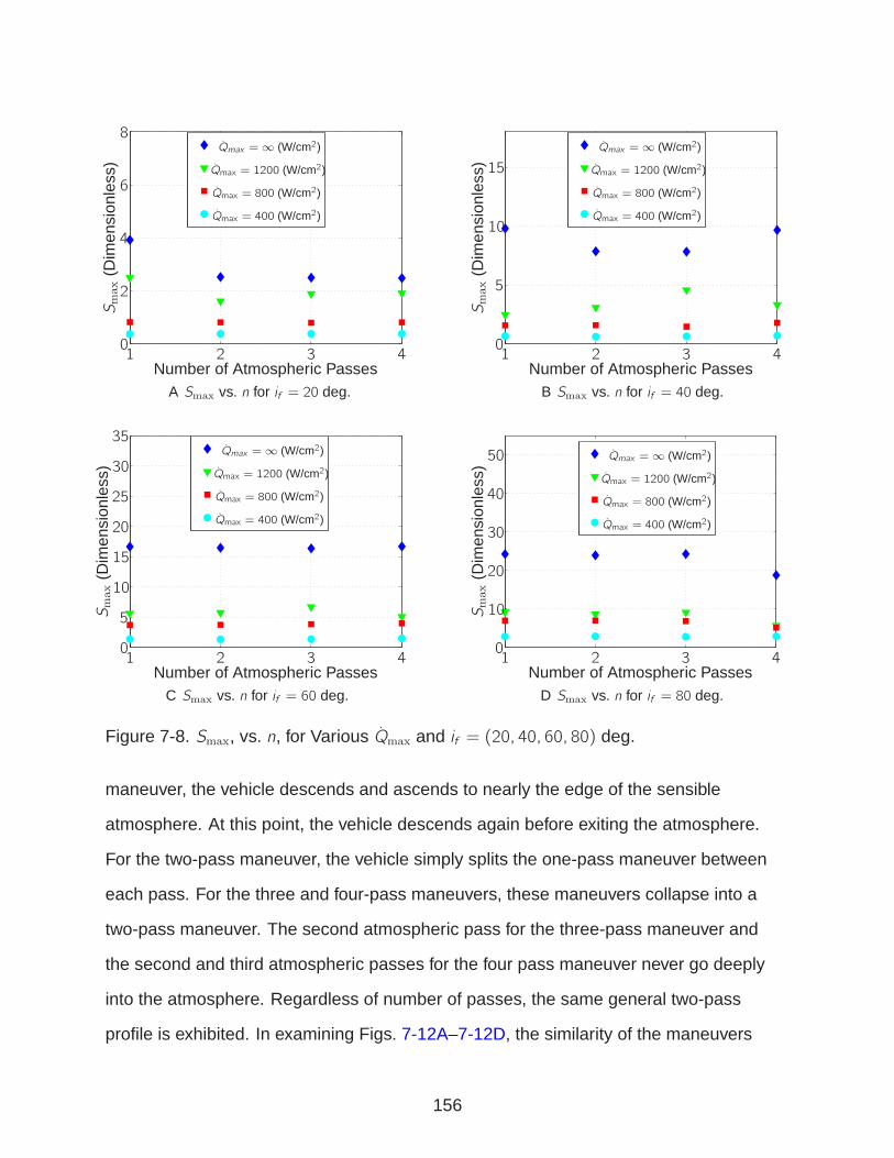
01 3
8
2
2
4
4
6
Number of Atmospheric Passes
Qmax =∞ (W/cm2)
Qmax = 1200 (W/cm2)
Qmax = 800 (W/cm2)
Qmax = 400 (W/cm2)
Smax
(Dim
ensi
onle
ss)
A Smax vs. n for if = 20 deg.
01 3
5
15
2 4
10
Number of Atmospheric Passes
Qmax =∞ (W/cm2)
Qmax = 1200 (W/cm2)
Qmax = 800 (W/cm2)
Qmax = 400 (W/cm2)
Smax
(Dim
ensi
onle
ss)
B Smax vs. n for if = 40 deg.
01 3
5
25
35
30
15
2 4
10
20
Number of Atmospheric Passes
Qmax =∞ (W/cm2)
Qmax = 1200 (W/cm2)
Qmax = 800 (W/cm2)
Qmax = 400 (W/cm2)
Smax
(Dim
ensi
onle
ss)
C Smax vs. n for if = 60 deg.
01 3
30
50
2 4
10
40
20
Number of Atmospheric Passes
Qmax =∞ (W/cm2)
Qmax = 1200 (W/cm2)
Qmax = 800 (W/cm2)
Qmax = 400 (W/cm2)
Smax
(Dim
ensi
onle
ss)
D Smax vs. n for if = 80 deg.
Figure 7-8. Smax, vs. n, for Various Qmax and if = (20, 40, 60, 80) deg.
maneuver, the vehicle descends and ascends to nearly the edge of the sensible
atmosphere. At this point, the vehicle descends again before exiting the atmosphere.
For the two-pass maneuver, the vehicle simply splits the one-pass maneuver between
each pass. For the three and four-pass maneuvers, these maneuvers collapse into a
two-pass maneuver. The second atmospheric pass for the three-pass maneuver and
the second and third atmospheric passes for the four pass maneuver never go deeply
into the atmosphere. Regardless of number of passes, the same general two-pass
profile is exhibited. In examining Figs. 7-12A–7-12D, the similarity of the maneuvers
156
12
Alti
tude
(km
)
Velocity (km/s)5 7 118 96 10
40
60
80
100
120
20
Qmax =∞ (W/cm2)
Qmax = 800 (W/cm2)
Qmax = 400 (W/cm2)
A h, vs. v .
Time (sec)
Q(W
/cm2)
00
1000
1000
1500
1500
2000
2000
2500
2500
3000
3000 3500
500
500
Qmax =∞ (W/cm2)
Qmax = 800 (W/cm2)
Qmax = 400 (W/cm2)
B Q, vs. t for if = 40-deg.
Alti
tude
(km
)
γ (deg)0 5−5 10
40
60
80
100
120
20
Qmax =∞ (W/cm2)
Qmax = 800 (W/cm2)
Qmax = 400 (W/cm2)
C h vs. γ.
Figure 7-9. h vs. v , Q vs. t, and h vs. γ for if = 40-deg.
regardless of number of passes is seen again in examining the heating rate versus time
in the atmosphere. Regardless of number of passes, the same heating rate profile is
seen. The first time the maximum value of the heating rate is met, the vehicle rides
along the maximum value of the heating rate and then reascends. The second time the
vehicle achieves the maximum value of the heating rate constraint, it only touches it
before reascending. Again, it is seen that the interior passes for the three and four-pass
maneuvers collapse into passes that do not descend far into the atmosphere.
157

Time (sec)
Ang
leof
Atta
ck(D
eg)
00
30
50
1000 1500 2000 2500 3000 3500
10
500
40
20
Qmax =∞ (W/cm2)
Qmax = 800 (W/cm2)
Qmax = 400 (W/cm2)
A α vs. t.
Time (sec)
Ban
kA
ngle
(Deg
)
0
0
−100
−2001000 1500 2000 2500 3000 3500
200
500
100
Qmax =∞ (W/cm2)
Qmax = 800 (W/cm2)
Qmax = 400 (W/cm2)
B σ vs. t.
Figure 7-10. α and σ vs. t for n = 1 and if = 40 deg.
158

Alti
tude
(km
)
7 7.5 8 8.5 9 9.540
60
80
100
120
Velocity (km/s)A h vs. v for n = 1 and if = 40 deg.
Alti
tude
(km
)
7 7.5 8 8.5 9 9.540
60
80
100
120
Velocity (km/s)
First Pass
Second Pass
B h vs. v for n = 2 and if = 40 deg.
Alti
tude
(km
)
7 7.5 8 8.5 9 9.540
60
80
100
120
Velocity (km/s)
First Pass
Second Pass
Third Pass
C h vs. v for n = 3 and if = 40 deg.
Alti
tude
(km
)
7 7.5 8 8.5 9 9.540
60
80
100
120
Velocity (km/s)
First Pass
Second Pass
Third Pass
Fourth Pass
D h vs. v for n = 2 and if = 40 deg.
Figure 7-11. h vs. v for n = (1, 2, 3, 4) and if = 40 deg and Qmax = 400 (W/cm2).
7.6 Discussion
The results of this study demonstrate several interesting features of using
aeroassisted glide maneuvers to change the inclination of a small spacecraft in LEO. For
an unconstrained heating rate, it is demonstrated that the total fuel required to change
the inclination of the small spacecraft is much less than for an all-propulsive maneuver.
As the heating rate is tightened, the cost of the aeroassisted maneuvers increase, but,
are still more efficient than the all-propulsive maneuvers except for the single case of
if = 80 degrees and Qmax = 400W/cm2. For an unconstrained heating rate, regardless
159

Q(W
/cm2)
00 1000 1500 2000 2500 3000
200
400
500
500
100
300
Time Since Atmospheric Entry (sec)A Q vs. t for n = 1 and if = 40 deg.
Q(W
/cm2)
00 1000 1500 2000 2500 3000
200
400
500
500
100
300
First Pass
Second Pass
Time Since Atmospheric Entry (sec)B Q vs. t for n = 2 and if = 40 deg.
Q(W
/cm2)
00 1000 1500 2000 2500 3000
200
400
500
500
100
300
First Pass
Second Pass
Third Pass
Time Since Atmospheric Entry (sec)C Q vs. t for n = 3 and if = 40 deg.
Q(W
/cm2)
00 1000 2000 3000
200
400
4000 5000
500
100
300
First Pass
Second Pass
Third Pass
Fourth Pass
Time Since Atmospheric Entry (sec)D Q vs. t for n = 4 and if = 40 deg.
Figure 7-12. Q, vs. t for n = (1, 2, 3, 4), if = 40 deg and Qmax = 400 (W/cm2).
of number of atmospheric passes, the vehicle dives deeply into the atmosphere only
once and affects all of the inclination change with this single atmospheric dive. For
the constrained heating rate cases, it is demonstrated that regardless of number of
atmospheric passes, the vehicle essentially conducts a two-pass maneuver. In the
first pass, the vehicle dives into the atmosphere and rides the heating rate constraint
for a finite duration. In the second pass, the vehicle merely touches the heating rate
constraint before reascending.
160

7.7 Conclusions
A study has been given on changing the inclination of a small high lift-to-drag ratio
spacecraft in low-Earth orbit using aeroassisted maneuvers. Three velocity impulses
(a de-orbit, boost, and re-circularization) are used along with lift and drag forces in the
atmosphere to change the inclination of the vehicle. It is found that the optimal solution
is insensitive to the number of atmospheric passes. For an unconstrained heating rate,
the solution reduces to a one-pass maneuver regardless of number of passes. For
highly constrained heating rates, the solution reduces to a two-pass maneuver. Finally,
it was found that for all but the highest inclination changes with the tightest heating rate
constraints that an aeroassisted maneuver was more fuel efficient than an all-propulsive
maneuver.
161
CHAPTER 8CONCLUSIONS
8.1 Dissertation Summary
Numerical methods for solving optimal control problems fall into two categories:
indirect and direct methods. An indirect method solves the continuous-time first-order
necessary conditions from the calculus of variations. While indirect methods in general
provide high-accuracy approximations, it is often hard to find a solution to these
necessary conditions. Direct collocation methods, on the other hand, are a more
robust numerical approximation technique. Direct collocation methods discretize the
original continuous-time optimal control problem such that the infinite-dimensional
continuous-time problem is transcribed into a finite-dimensional discrete problem, or
nonlinear programming problem (NLP). Direct methods have most commonly been
applied as h–methods. An h–method uses many low-degree approximating subintervals
and guarantees that the NLP is sparse. In contrast to h–methods, p–methods use a few
fixed number of intervals with a variable degree polynomial in each interval. A p–method
results in a dense NLP, but, if the solution to a problem is simple and smooth, high
accuracy approximations to the continuous-time optimal control problem are obtained
with small NLPs.
In this dissertation, an hp–direct collocation method has been presented. The
hp–method allows for a variable number of approximating intervals with a variable
degree approximation within each interval. The result is a method that is robust with
respect to the solution structure of a problem (that is, some optimal control problems are
better approximated by an h–biased method, while other optimal control problems are
better approximated by a p–biased method). The discrete approximation in each interval
is defined by the set of Legendre-Gauss or Legendre-Gauss-Radau points. These
points are used because they are defined by highly accurate quadrature rules and when
used as the support points in a Lagrange polynomial, do not exhibit Runge phenomenon
162
for high-degree approximations. Next, in analyzing the KKT conditions of the NLP, it
is found that the hp–method of this research results in a discrete representation of the
continuous-time first-order optimality conditions if the costate is continuous.
Two hp–mesh refinement algorithms have been presented. In each algorithm, the
accuracy of the approximation in each mesh interval is assessed by evaluating the
differential-algebraic constraints between collocation points. If an approximating interval
is inaccurate, the interval is modified by either increasing the degree of approximation
within the interval, or by subdividing the interval. The hp–mesh refinement algorithms
iteratively update the approximating grid until an approximation is accurate in every
approximating interval. The hp–mesh refinement algorithms are capable of utilizing
the best approximation strategy for different regions of a solution by modifying the
mesh either by increasing the degree of the approximating polynomial or increasing
the number of mesh intervals. The two hp–mesh refinement algorithms presented
in this research are distinctly different from one another because the first algorithm
is a p–biased algorithm while the second algorithm is an h–biased algorithm. Both
algorithms are compared with one another along with comparisons to p and h–methods
over several examples. It is demonstrated that the hp–methods are robust to problem
type and accurately solve the problems presented in a computationally efficient manner.
Furthermore, hp–mesh refinement algorithm 2 is the most successful strategy when
compared with p, h, and hp–mesh refinement algorithm 1 over the range of problems.
Utilizing the computational sparsity of an h–method as a starting point, hp–mesh
refinement algorithm 2 results in a sparse NLP. Furthermore, by using mid-degree
collocation only on smooth intervals, high accuracy approximations are obtained in a
computationally efficient manner. hp–mesh refinement algorithm 2 provides accurate
approximations to continuous-time optimal control problems with simultaneously small
and sparse NLPs.
163
Finally, an optimal aeroassisted orbital inclination change maneuver is studied.
In this study, a small maneuverable spacecraft in low-Earth orbit (LEO) uses the
aerodynamic forces of lift and drag to change the orbital inclination. The maneuver
is studied for a multiple number of atmospheric passes and variable heating rate
constraints. The aeroassisted maneuvers is demonstrated to be more fuel efficient
than all-propulsive inclination change maneuvers. Furthermore, it is found that the
aeroassisted maneuvers are insensitive to number of atmospheric passes.
8.2 Future Work
8.2.1 Continued Work on Mesh Refinement
Two hp–mesh refinement algorithms have been presented in this research. It is
believed that automatic mesh generation is a rich subject and many more advances
may be made. Typically, mesh refinement strategies are studied for h–methods. In
an h–method, there are only two degrees of freedom in refining a mesh, namely, the
number of mesh intervals and the placement of the mesh points. hp–mesh refinement
algorithms are significantly more complex, however, because there are three degrees
of freedom for refining a mesh, namely, the number of mesh intervals, the placement of
the mesh points, and the degree of the approximating polynomial within each interval.
Because of this extra degree of freedom in generating an approximating mesh, the
choice of how to refine a mesh is more complicated, but also more interesting and
fruitful. Presented in this research are two static refinement algorithms that only
increase the size of the NLP on every iteration. Two interesting future concepts to
explore are now stated. The first concept is a refinement process to decrease the size
of the NLP if any intervals are more accurate than the desired accuracy level, further
increasing the computational efficiency of the NLP. The second concept is to add a
dynamic mesh refinement component that can be used to exactly locate the switch in
activity between active and inactive path constraints. One of the strengths of a direct
collocation method is that the location of active and inactive constraint arcs does not
164
need to be known in order to approximate the solution of the problem. If the locations of
these arcs can be determined, however, the approximations can be made significantly
more accurate.
8.2.2 Discontinuous Costate
It has been demonstrated in this research that high-accuracy approximations are
achieved by the proposed hp–method if the costate is continuous. If mesh points are
at the location of discontinuity in the costate, the transformed adjoint system is an
inexact discrete representation of the continuous-time first-order necessary conditions.
For a dynamic refinement algorithm that will exactly locate the switch in activity of
inequality path constraints, it is likely that the costate may be discontinuous at mesh
points. It is necessary to determine how to make the transformed adjoint system a
discrete representation of the continuous-time first-order necessary conditions for a
discontinuous costate solution if mesh points are at the location of discontinuity in the
costate.
165
REFERENCES
[1] Kirk, D. E., Optimal Control Theory: An Introduction, Dover Publications, Mineola,New York, 2004.
[2] Bryson, A. E. and Ho, Y.-C., Applied Optimal Control , Hemisphere Publishing, NewYork, 1975.
[3] Pontryagin, L. S., Mathematical Theory of Optimal Processes, John Wiley & Sons,New York, 1962.
[4] Betts, J. T., “Survey of Numerical Methods for Trajectory Optimization,” Journal ofGuidnance, Control, and Dynamics, Vol. 21, No. 2, March–April 1998, pp. 193–207.
[5] von Stryk, O. and Bulirsch, R., “Direct and Indirect Methods for TrajectoryOptimization,” Annals of Operations Research, Vol. 37, 1992, pp. 357–373.
[6] Oberle, H. J. and Grimm, W., “BNDSCO: A Program for the Numerical Solutionof Optimal Control Problems,” Tech. rep., Institute of Flight Systems Dynamics,German Aerospace Research Establishment DLR, IB 515-89/22, Oberpfaffenhofen,Germany, 1990.
[7] Press, W. H., Flannery, B. P., Teukolsky, S., and Vetterling, W. T., NumericalRecipes: The Art of Scientific Computing, Cambridge University Press, 1990.
[8] Keller, H. B., Numerical Solution of Two Point Boundary Value Problems, SIAM,1976.
[9] Dickmanns, E. D. and Well, K. H., “Approximate Solution of Optimal ControlProblems Using Third Order Hermite Polynomial Functions,” Lecture Notes inComputational Science, Springer , Vol. 27, 1975.
[10] Russell, R. D. and Shampine, L. F., “A Collocation Method for Boundary ValueProblems,” Numerical Mathematics, Vol. 19, No. 1, 1972, pp. 1–28.
[11] Gill, P. E., Murray, W., and Saunders, M. A., “SNOPT: An SQP Algorithm forLarge-Scale Constrained Optimization,” SIAM Review , Vol. 47, No. 1, January2002, pp. 99–131.
[12] Biegler, L. T. and Zavala, V. M., “Large-Scale Nonlinear Programming Using IPOPT:An Integrating Framework for Enterprise-Wide Optimization,” Computers andChemical Engineering, Vol. 33, No. 3, March 2008, pp. 575–582.
[13] Byrd, R. H., Nocedal, J., and Waltz, R. A., “KNITRO: An Integrated Package forNonlinear Optimization,” Large Scale Nonlinear Optimization, Springer Verlag,2006, pp. 35–59.
166

[14] Kraft, D., On Converting Optimal Control Problems into Nonlinear ProgrammingCodes, Vol. F15 of NATO ASI Series, in Computational Mathematical Program-ming, Springer-Verlag, Berlin, 1985, pp. 261–280.
[15] Bock, H. G. and Plitt, K. J., “A Multiple Shooting Algorithm for Direct Solution ofOptimal Control Problems,” IFAC 9th World Congress, Budapest, Hungary, 1984.
[16] Schwartz, A., Theory and Implementation of Numerical Methods Based on Runge-Kutta Integration for Solving Optimal Control Problems, Ph.D. thesis, Department ofElectrical Engineering, University of California, Berkeley, 1996.
[17] Brauer, G. L., Cornick, D. E., and Stevenson, R., “Capabilities and Applications ofthe Program to Optimize and Simulate Trajectories,” Tech. Rep. NASA-CR-2770,National Aeronautics and Space Administration, 1977.
[18] Hargraves, C. R. and Paris, S. W., “Direct Trajectory Optimization Using NonlinearProgramming Techniques,” Journal of Guidance, Control, and Dynamics, Vol. 10,No. 4, July–August 1987, pp. 338–342.
[19] Betts, J., Practical Methods for Optimal Control and Estimation Using NonlinearProgramming, SIAM Press, Philadelphia, 2nd ed., 2009.
[20] Enright, P. J. and Conway, B. A., “Discrete Approximations to Optimal TrajectoriesUsing Direct Transcription and Nonlinear Programming,” Journal of Guidance,Control, and Dynamics, Vol. 19, No. 4, July–August 1996, pp. 994–1002.
[21] Hager, W. W., “Runge-Kutta Methods in Optimal Control and the TransformedAdjoint System,” Numerische Mathematik , Vol. 87, 2000, pp. 247–282.
[22] Benson, D. A., A Gauss Pseudospectral Transcription for Optimal Control, Ph.D.thesis, Department of Aeronautics and Astronautics, Massachusetts Institute ofTechnology, Cambridge, Massachusetts, 2004.
[23] Huntington, G. T., Benson, D. A., and Rao, A. V., “Optimal Configuration ofTetrahedral Spacecraft Formations,” The Journal of the Astronautical Sciences,Vol. 55, No. 2, April-June 2007, pp. 141–169.
[24] Betts, J. T. and Huffman, W. P., “Sparse Optimal Control Software – SOCS,” Tech.Rep. MEA-LR-085, Boeing Information and Support Services, Seattle, Washington,July 1997.
[25] von Stryk, O., User’s Guide for DIRCOL Version 2.1: A Direct Collocation Methodfor the Numerical Solution of Optimal Control Problems, Technische UniversitatDarmstadt, Darmstadt, Germany, 1999.
167
[26] Rao, A. V., Benson, D. A., Darby, C. L., Francolin, C., Patterson, M. A., Sanders,I., and Huntington, G. T., “Algorithm 902: GPOPS, A Matlab Software for SolvingMultiple-Phase Optimal Control Problems Using the Gauss PseudospectralMethod,” ACM Transactions on Mathematical Software, Vol. 37, No. 2, April–June2010, pp. 22:1–22:39.
[27] Dontchev, A. L., Hager, W. W., and Malanowski, K., “Error Bounds for the EulerApproximation and Control Constrained Optimal Control Problem,” NumericalFunctional Analysis and Applications, Vol. 21, 2000, pp. 653–682.
[28] Dontchev, A. L., Hager, W. W., and Veliov, V. M., “Second-Order Runge-KuttaApproximations In Constrained Optimal Control,” SIAM Journal on NumericalAnalysis, Vol. 38, 2000, pp. 202–226.
[29] Dontchev, A. L. and Hager, W. W., “The Euler Approximation in State ConstrainedOptimal Control,” Mathematics of Computation, Vol. 70, 2001, pp. 173–203.
[30] Zhao, Y. and Tsiotras, P., “A Density-Function Based Mesh Refinement Algorithmfor Solving Optimal Control Problems,” Infotech and Aerospace Conference, AIAAPaper 2009-2019, Seattle, Washington, April 2009.
[31] Jain, D. and Tsiotras, P., “Trajectory Optimization Using Multiresolution Techniques,”Journal of Guidance, Control, and Dynamics, Vol. 31, No. 5, September-October2008, pp. 1424–1436.
[32] Betts, J. T. and Erb, S. O., “Optimal Low Thrust Trajectories to the Moon,” SIAMJ. Appl. Dyn. Syst , Vol. 2, 2003, pp. 144–170.
[33] Elnagar, G., Kazemi, M., and Razzaghi, M., “The Pseudospectral Legendre Methodfor Discretizing Optimal Control Problems,” IEEE Transactions on AutomaticControl , Vol. 40, No. 10, 1995, pp. 1793–1796.
[34] Elnagar, G. and Razzaghi, M., “A Collocation-Type Method for Linear QuadraticOptimal Control Problems,” Optimal Control Applications and Methods, Vol. 18,No. 3, 1998, pp. 227–235.
[35] Benson, D. A., Huntington, G. T., Thorvaldsen, T. P., and Rao, A. V., “DirectTrajectory Optimization and Costate Estimation via an Orthogonal CollocationMethod,” Journal of Guidance, Control, and Dynamics, Vol. 29, No. 6,November-December 2006, pp. 1435–1440.
[36] Huntington, G. T., Advancement and Analysis of a Gauss Pseudospectral Tran-scription for Optimal Control , Ph.D. thesis, Massachusetts Institute of Technology,Cambridge, Massachusetts, 2007.
[37] Rao, A. V., Benson, D. A., Darby, C. L., Patterson, M. A., Sanders,I., and Huntington, G. T., User’s Manual for GPOPS Version 2.2,http://gpops.sourceforge.net/, June 2009.
168

[38] Kameswaran, S. and Biegler, L. T., “Convergence Rates for Direct Transcriptionof Optimal Control Problems Using Collocation at Radau Points,” ComputationalOptimization and Applications, Vol. 41, No. 1, 2008, pp. 81–126.
[39] Garg, D., Patterson, M. A., Darby, C. L., Francolin, C., Huntington, G. T.,Hager, W. W., and Rao, A. V., “Direct Trajectory Optimization and CostateEstimation of Finite-Horizon and Infinite-Horizon Optimal Control Problems viaa Radau Pseudospectral Method,” Computational Optimization and Applica-tions, Published Online: October 6, 2009. DOI 10.1007/s10589-009-9291-0.http://www.springerlink.com/content/n851q6n343p9k60k/.
[40] Garg, D., Patterson, M. A., Hager, W. W., Rao, A. V., Benson, D. A., and Huntington,G. T., “A Unified Framework for the Numerical Solution of Optimal Control ProblemsUsing Pseudospectral Methods,” Automatica, Published Online, August 2010.DOI:10.1016/j.automatica.2010.06.048.
[41] Fahroo, F. and Ross, I., “A Spectral Patching Method for Direct TrajectoryOptimization,” Journal of Astronautical Sciences, Vol. 48, No. 2-3, Apr.-Sept.2000, pp. 269–286.
[42] Fahroo, F. and Ross, I., “Costate Estimation by a Legendre PseudospectralMethod,” Journal of Guidance, Control, and Dynamics, Vol. 24, No. 2, 2001,pp. 270–277.
[43] Fahroo, F. and Ross, I., “Direct Trajectory Optimization by a ChebyshevPseudospectral Method,” Journal of Guidance, Control, and Dynamics, Vol. 25,No. 1, 2002, pp. 160–166.
[44] Fahroo, F. and Ross, I., “Pseudospectral Methods for Infinite-Horizon NonlinearOptimal Control Problems,” Journal of Guidance, Control, and Dynamics, Vol. 31,No. 4, 2008, pp. 927–936.
[45] Gong, Q., Kang, W., and Ross, I. M., “A Pseudospectral Method for the OptimalControl of Feedback Linearizable Systems,” IEEE Transactions on AutomaticControl , Vol. 51, No. 7, July 2006, pp. 1115–1129.
[46] Gong, Q., Ross, I. M., Kang, W., and Fahroo, F., “Connections Between theCovector Mapping Theorem and Convergence of Pseudospectral Methods,”Computational Optimization and Applications, Vol. 41, No. 3, December 2008,pp. 307–335.
[47] Gong, Q., Fahroo, F., and Ross, I. M., “Spectral Algorithm for PseudospectralMethods in Optimal Control,” Journal of Guidance, Control, and Dynamics, Vol. 31,No. 3, May-June 2008.
[48] Ross, I. and Fahroo, F., “Pseudospectral Knotting Methods for Solving OptimalControl Problems,” Journal of Guidance, Control, and Dynamics, Vol. 27, No. 3,2004, pp. 397–405.
169
[49] Ross, I. M. and Fahroo, F., “Legendre Pseudospectral Approximations ofOptimal Control Problems,” Lecture Notes in Control and Information Sciences,Springer-Verlag, 2003, pp. 327–342.
[50] Ross, I. and Fahroo, F., “Advances in Pseusospectral Methods for Optimal Control,”AIAA Guidance, Navigation, and Control Conference, AIAA Paper 2008-7309,Honolulu, Hawaii, August 2008.
[51] Ross, I. and Fahroo, F., “Convergence of the Costates Does Not ImplyConvergence of the Controls,” Journal of Guidance, Control, and Dynamics,Vol. 31, No. 4, 2008, pp. 1492–1497.
[52] Ross, I. M. and Fahroo, F., User’s Manual for DIDO 2001 α: A MATLAB Applicationfor Solving Optimal Control Problems, Department of Aeronautics and Astronautics,Naval Postgraduate School, Technical Report AAS-01-03, Monterey, California,2001.
[53] Canuto, C., Hussaini, M. Y., Quarteroni, A., and Zang, T. A., Spectral Methods inFluid Dynamics, Spinger-Verlag, Heidelberg, Germany, 1988.
[54] Fornberg, B., A Practical Guide to Pseudospectral Methods, Cambridge UniversityPress, 1998.
[55] Trefethen, L. N., Spectral Methods Using MATLAB, SIAM Press, Philadelphia,2000.
[56] Babuska, I. and Suri, M., “The p and hp Version of the Finite Element Method, anOverview,” Computer Methods in Applied Mechanics and Engineering, Vol. 80,1990, pp. 5–26.
[57] Babuska, I. and Suri, M., “The p and hp Version of the Finite Element Method,Basic Principles and Properties,” SIAM Review , Vol. 36, 1994, pp. 578–632.
[58] Gui, W. and Babuska, I., “The h, p, and hp Versions of the Finite Element Method in1 Dimension. Part I. The Error Analysis of the p Version,” Numerische Mathematik ,Vol. 49, 1986, pp. 577–612.
[59] Gui, W. and Babuska, I., “The h, p, and hp Versions of the Finite Element Method in1 Dimension. Part II. The Error Analysis of the h and h − p Versions,” NumerischeMathematik , Vol. 49, 1986, pp. 613–657.
[60] Gui, W. and Babuska, I., “The h, p, and hp Versions of the Finite Element Method in1 Dimension. Part III. The Adaptive h−p Version,” Numerische Mathematik , Vol. 49,1986, pp. 659–683.
[61] Betts, J. T. and Huffman, W. P., “Mesh Refinement in Direct Transcription Methodsfor Optimal Control,” Optimal Control Applications and Methods, Vol. 19, 1998,pp. 1–21.
170

[62] Atkinson, K. E., An Introduction to Numerical Analysis, John Wiley and Sons, NewYork, NY, 1989.
[63] Davis, P. J. and Rabinowitz, P., Methods of Numerical Integration, Academic Press,New York, 1984.
[64] Soueres, P. and Boissonnat, J. D., Robot Motion Planning and Control, Springer,Englewood Cliffs, NJ, 1998.
[65] Meditch, J., “On the Problem of Optimal Thrust Programming for a Soft LunarLanding,” IEEE Transaction on Automatic Control , Vol. 9, No. 4, 1964, pp. 477–484.
[66] Darby, C. L., Hager, W. W., and Rao, A. V., “An hp-Adaptive Pseudospectral Methodfor Solving Optimal Control Problems,” Optimal Control Applications and Methods,August 2010.
[67] Darby, C. L., Hager, W. W., and Rao, A. V., “Direct Trajectory Optimization by AVariable Low-Order hp-Adaptive Pseudospectral Method,” Journal of Spacecraftand Rockets, Accepted for Publication November 2010 (in press).
[68] Gill, P. E., Murray, W., and Saunders, M. A., User’s Guide for SNOPT Version 7:Software for Large Scale Nonlinear Programming, February 2006.
[69] Betts, J. T., Practical Methods for Optimal Control and Estimation Using NonlinearProgramming, SIAM Press, Philadelphia, 2010.
[70] Rao, A. V. and Mease, K. D., “Dichotomic Basis Approach to solvingHyper-Sensitive Optimal Control Problems,” Automatica, Vol. 35, No. 4, April1999, pp. 633–642.
[71] Rao, A. V. and Mease, K. D., “Eigenvector Approximate Dichotomic Basis Methodfor Solving Hyper-Sensitive optimal Control Problems,” Optimal Control Applicationsand Methods, Vol. 21, No. 1, January–February 2000, pp. 1–19.
[72] Rao, A. V., “Application of a Dichotomic Basis Method to Performance Optimizationof Supersonic Aircraft,” Journal of Guidance, Control, and Dynamics, Vol. 23, No. 3,May–June 2000, pp. 570–573.
[73] Rao, A. V., “Riccati Dichotomic Basis Method for solving Hyper-Sensitive optimalControl Problems,” Journal of Guidance, Control, and Dynamics, Vol. 26, No. 1,January–February 2003, pp. 185–189.
[74] Bryson, A. E., Desai, M. N., and Hoffman, W. C., “Energy-State Approximation inPerformance Optimization of Supersonic Aircraft,” AIAA Journal of Aircraft , Vol. 6,No. 6, 1969, pp. 481–488.
[75] Seywald, H. and Kumar, R. R., “Finite Difference Scheme for Automatic CostateCalculation,” Journal of Guidance, Control, and Dynamics, Vol. 19, No. 4, 1996,pp. 231–239.
171

[76] London, H. S., “Change of Satellite Orbit Plane by Aerodynamic Maneuvering,” IAS29th Annual Meeting, International Astronautical Society, New York, January 1961.
[77] Walberg, G. D., “A Survey of Aeroassisted Orbit Transfer,” Journal of Spacecraftand Rockets, Vol. 22, No. 1, 1985, pp. 3–18.
[78] Mease, K. D., “Aerossisted Orbital Transfer: Current Status,” The Journal of theAstronautical Sciences, Vol. 36, No. 1/2, 1988, pp. 7–33.
[79] Rao, A. V., Tang, S., and Hallman, W. P., “Numerical Optimization Study ofMultiple-Pass Aeroassisted Orbital Transfer,” Optimal Control Applications andMethods, Vol. 23, No. 4, July–August 2002, pp. 215–238.
[80] Darby, C. L. and Rao, A. V., “Minimum-Fuel Low-Earth Orbit Aeroassisted OrbitalTransfer of Small Spacecraft,” Journal of Spacecraft and Rockets, Accepted forPublication February 2011 (in press).
[81] Vinh, N.-X., Busemann, A., and Culp, R., Hypersonic and Planetary Entry FlightMechanics, Elsevier Science, New York, 1981.
[82] Clarke, K., Performance Optimization of a Common Aero Vehicle Using a LegendrePseudospectral Method , Ph.D. thesis, Department of Aeronautics and Astronautics,Massachusetts Institute of Technology, Cambridge, Massachusetts, 2003.
[83] Bate, R. R., Mueller, D. D., and White, J. E., Fundamentals of Astrodynamics, DoverPublications, 1971.
[84] Detra, R. W., Kemp, N. H., and Riddell, F. R., “Addendum to Heat Transfer ofSatellite Vehicles Re-entering the Atmosphere,” Jet Propulsion, Vol. 27, 1957,pp. 1256–1257.
[85] Rump, S. M., “INTLAB – INTerval LABoratory,” Developments in Reliable Com-puting, edited by T. Csendes, Kluwer Academic Publishers, Dordrecht, 1999, pp.77–104.
[86] Tewari, A., Atmospheric and Space Flight Dynamics, Birkhauser, Boston, 2007.
172

BIOGRAPHICAL SKETCH
Christopher Darby was born in 1983 in Gainesville, Florida. He received his
Bachelor of Science degree in mechanical engineering in December 2006, his Master of
Science degree in mechanical engineering in May 2010, and his Doctor of Philosophy
in mechanical engineering in May 2011. Each degree was earned at the University
of Florida. His research interests include numerical approximations to differential
equations, optimal control theory, and numerical approximations to the solution of
optimal control problems.
173