hrank: filter pruning using high-rank feature map
TRANSCRIPT

HRank: Filter Pruning using High-Rank Feature Map
Mingbao Lin1, Rongrong Ji1,5∗, Yan Wang2, Yichen Zhang1,
Baochang Zhang3, Yonghong Tian4,5, Ling Shao6
1Media Analytics and Computing Laboratory, Department of Artificial Intelligence, School of
Informatics, Xiamen University, China, 2Pinterest, USA, 3Beihang University, China4Peking University, Beijing, China, 5Peng Cheng Laboratory, Shenzhen, China
6Inception Institute of Artificial Intelligence, Abu Dhabi, UAE
[email protected], [email protected], [email protected], [email protected],
[email protected], [email protected], [email protected]
Abstract
Neural network pruning offers a promising prospect
to facilitate deploying deep neural networks on resource-
limited devices. However, existing methods are still chal-
lenged by the training inefficiency and labor cost in pruning
designs, due to missing theoretical guidance of non-salient
network components. In this paper, we propose a novel fil-
ter pruning method by exploring the High Rank of feature
maps (HRank). Our HRank is inspired by the discovery that
the average rank of multiple feature maps generated by a
single filter is always the same, regardless of the number of
image batches CNNs receive. Based on HRank, we develop
a method that is mathematically formulated to prune filters
with low-rank feature maps. The principle behind our prun-
ing is that low-rank feature maps contain less information,
and thus pruned results can be easily reproduced. Besides,
we experimentally show that weights with high-rank feature
maps contain more important information, such that even
when a portion is not updated, very little damage would be
done to the model performance. Without introducing any
additional constraints, HRank leads to significant improve-
ments over the state-of-the-arts in terms of FLOPs and pa-
rameters reduction, with similar accuracies. For example,
with ResNet-110, we achieve a 58.2%-FLOPs reduction by
removing 59.2% of the parameters, with only a small loss
of 0.14% in top-1 accuracy on CIFAR-10. With Res-50,
we achieve a 43.8%-FLOPs reduction by removing 36.7%of the parameters, with only a loss of 1.17% in the top-
1 accuracy on ImageNet. The codes can be available at
https://github.com/lmbxmu/HRank.
∗Corresponding author
1. Introduction
Convolutional Neural Networks (CNNs) have demon-
strated great success in computer vision applications, like
classification [33, 11], detection [7, 30], and segmentation
[25, 2]. However, their high demands in computing power
and memory footprint prohibit most state-of-the-art CNNs
to be deployed in edge devices such as smartphones or
wearable devices. While good progress has been made in
designing new hardware and/or hardware-specific CNN ac-
celeration frameworks like TensorRT, it retains as a signif-
icant demand to reduce the FLOPs and size of CNNs, with
limited compromise on accuracy [4]. Popular techniques
include filter compression [6], parameter quantization [3],
and network pruning [10].
Among them, network pruning has shown broad
prospects in various emerging applications. Typical works
either prune the filter weights to obtain sparse weight matri-
ces (weight pruning) [10, 9, 1], or remove entire filters from
the network (filter pruning) [18, 19, 20]. Besides network
compression, weight pruning approaches can also achieve
acceleration on specialized software [28] or hardware [8].
However, they have limited applications on general-purpose
hardware or BLAS libraries. In contrast, filter pruning ap-
proaches do not have this limitation since entire filters are
removed. In this paper, we focus on the filter pruning to
achieve model compression (reduction in parameters) and
acceleration (reduction in FLOPs), aiming to provide a ver-
satile solution for devices with low computing power.
The core of filter pruning lies in the selection of filters,
which should yield the highest compression ratio with the
lowest compromise in accuracy. Based on the design of
filter evaluation functions, we empirically categorize filter
pruning into two groups as discussed below.
1529
Property Importance: The filters are pruned based on
the intrinsic properties of CNNs. These pruning approaches
do not modify the network training loss. After the pruning,
the model performance is enhanced through fine-tuning.
Among these methods, Hu et al. [14] utilized the spar-
sity of outputs in a large network to remove filters with
a high percentage of zero activations. The ℓ1-norm based
pruning [18] assumes that parameters or features with small
norms are less informative, and thus should be pruned first.
Molchanov et al. [27] considered the first-order gradient
to evaluate the importance of filters and removed the least
important ones. In [34], the importance scores of the final
responses are propagated to every filter in the network and
the CNNs are pruned by removing the one with the least im-
portance. He et al. [12] calculated the geometric median in
the layers, and the filters closest to this are pruned. Most de-
signs for filter evaluation functions are ad-hoc, which brings
the advantage of low time complexity, but also limits the ac-
celeration and compression ratios.
Adaptive Importance: Different from the property im-
portance based approaches, another direction embeds the
pruning requirement into the network training loss, and em-
ploys a joint-retraining optimization to generate an adaptive
pruning decision. Liu et al. [24] and Zhao et al. [36] im-
posed a sparsity constraint on the scaling factor of the batch
normalization layer, allowing channels with lower scaling
factors to be identified as unimportant. Huang et al. [16]
and Lin et al. [23] introduced a new scaling factor pa-
rameter (also known as a mask) to learn a sparse struc-
ture pruning where filters corresponding to a scaling fac-
tor of zero are removed. Compared with property impor-
tance based filter pruning, adaptive importance based meth-
ods usually yield better compression and acceleration re-
sults due to their joint optimization. However, because the
loss is changed, the required retraining step is heavy in both
machine time and human labor, usually demanding another
round of hyper-parameter tuning. For some methods, e.g.,
the mask-based scheme, the modified loss even requires
specialized optimizers [16, 23], which affects the flexibility
and ease of using approaches based on adaptive importance.
Overall, filter pruning remains an open problem so far.
On one hand we pursuit higher compression/acceleration
ratios, while on the other hand we are restricted by heavy
machine time and human labor (especially for adaptive im-
portance based methods). We attribute these problems to the
lack of practical/theoretical guidance regarding to the filter
importance and redundancy. In this paper, we propose an
effective and efficient filter pruning approach that explores
the High Rank of the feature map in each layer (HRank), as
shown in Fig. 1. The proposed HRank performs as such
a guidance, which is a property importance based filter
pruner. It eliminates the need of introducing additional aux-
iliary constraints or retraining the model, thus simplifying
Feature Map
Generation
𝜹
rank
Fine-Tuning/Inference Phase
…
FilterSelection
…
…
…
…
…
rank
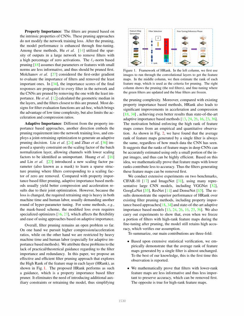
Figure 1. Framework of HRank. In the left column, we first use
images to run through the convolutional layers to get the feature
maps. In the middle column, we then estimate the rank of each
feature map, which is used as the criteria for pruning. The right
column shows the pruning (the red filters), and fine-tuning where
the green filters are updated and the blue filters are frozen.
the pruning complexity. Moreover, compared with existing
property importance based methods, HRank also leads to
significant improvements in acceleration and compression
[18, 34] , achieving even better results than state-of-the-art
adaptive importance based methods [13, 24, 26, 16, 23, 36].
The motivation behind enforcing the high rank of feature
maps comes from an empirical and quantitative observa-
tion. As shown in Fig. 2, we have found that the average
rank of feature maps generated by a single filter is always
the same, regardless of how much data the CNN has seen.
It suggests that the ranks of feature maps in deep CNNs can
be accurately estimated using only a small portion of the in-
put images, and thus can be highly efficient. Based on this
idea, we mathematically prove that feature maps with lower
ranks contribute less to accuracy. Thus the filters generating
these feature maps can be removed first.
We conduct extensive experiments on two benchmarks,
CIFAR-10 [17] and ImageNet [31], using many repre-
sentative large CNN models, including VGGNet [32],
GoogLeNet [33], ResNet [11] and DenseNet [15]. The re-
sults demonstrate the superior performance of HRank over
existing filter pruning methods, including property impor-
tance based approaches[18, 34] and state-of-the-art adaptive
importance based models [13, 24, 26, 16, 23, 36]. We also
carry out experiments to show that, even when we freeze
a portion of filters with high-rank feature maps during the
fine-tuning after pruning, the model still retains high accu-
racy, which verifies our assumption.
To summarize, our main contributions are three-fold:
• Based upon extensive statistical verification, we em-
pirically demonstrate that the average rank of feature
maps generated by a single filter is almost unchanged.
To the best of our knowledge, this is the first time this
observation is reported.
• We mathematically prove that filters with lower-rank
feature maps are less informative and thus less impor-
tant to preserve accuracy, which can be removed first.
The opposite is true for high-rank feature maps.
1530

• Extensive experiments demonstrate the efficiency and
effectiveness of HRank in both model compression and
acceleration over a variety of state-of-the-arts [18, 34,
13, 24, 26, 16, 23, 36].
2. Related Work
Filter Pruning. Opposed to weight pruning, which
prunes the weight matrices, filter pruning removes the en-
tire filters according to certain metrics. Filter pruning not
only significantly reduces storage usage, but also decreases
the computational cost in online inference. As discussed
in Sec. 1, filter pruning can be divided into two categories:
property importance approaches and adaptive importance
approaches. Property importance based filter pruning aims
to exploit the intrinsic properties of CNNs (e.g., ℓ1-norm
and gradient, etc), and then uses them as criteria for discrim-
inating less important filters. For example, the sparser fil-
ters in [27] are considered less important while [14] prunes
filters with smaller ℓ1-norm. In contrast, adaptive impor-
tance based filter pruning typically retrain the networks with
additional constraints to generate an adaptive pruning deci-
sion. Beyond the related work discussed in Sec. 1, Luo et al.
[26] established filter pruning as an optimization problem,
where the filters are pruned based on the statistics informa-
tion from the next layer. He et al. [13] proposed a two-step
algorithm including a LASSO regression to remove redun-
dant filters and a linear least square to construct the outputs.
Low-rank Decomposition. As shown in [5], neural net-
works tend to be over-parameterized, which suggests that
the parameters in each layer can be accurately recovered
from a small subset. Inspired by this, low-rank decomposi-
tion has emerged as an alternative for network compression.
It approximates convolutional operations by representing
the weight matrix as a low-rank product of two smaller ma-
trices. Unlike pruning, it aims to reduce the computational
costs of the network instead of changing the original num-
ber of filters. To this end, Denton et al. [6] exploited the
linear structure of CNNs by exploring an appropriate low-
rank approximation of the weights and keeping the accuracy
within a 1% loss of the original model. Further, Zhang et
al. [35] considered the subsequent nonlinear units while
learning the low-rank decomposition to provide significant
speed-up. Lin et al. [21] proposed a low-rank decomposi-
tion for both convolutional filters and fully-connected ma-
trices, which are then solved by a closed-form solver with
a fixed rank. Though low-rank decomposition can benefit
the compression and speedup of CNNs, it normally incurs a
large loss in accuracy under high compression ratios.
Discussion. Compared with weight pruning, filter prun-
ing tends to be more favorable in reducing model complex-
ity. Besides, its structured pruning can be easily integrated
into the highly efficient BLAS libraries without specialized
software or hardware support. Nevertheless, existing fil-
ter pruning methods suffer from inefficient acceleration and
compression (property importance based filter pruning) or
machine and labor costs (adaptive importance based filter
pruning), as discussed in Sec. 1. These two issues bring
fundamental challenges to the deployment of deep CNNs on
resource-limited devices. We attribute the dilemma to the
missing of practical/theoretical guidance regarding to the
filter importance and redundancy. We focus on the rank of
feature maps and analyze its effectiveness both theoretically
and experimentally. Note that our approach is orthogonal
to low-rank decomposition approaches. We aim to prune
filters generating low-rank feature maps rather than decom-
pose filters. Note that, the low-rank methods can be inte-
grated into our model (e.g., to decompose fully-connected
layers) to achieve higher compression and speedup ratios.
3. The Proposed Method
3.1. Notations
Assume a pre-trained CNN model has a set of K con-
volutional layers1, and Ci is the i-th convolutional layer.
The parameters in Ci can be represented as a set of 3-
D filters WCi = {wi1,w
i2, ...,w
ini} ∈ R
ni×ni−1×ki×ki ,
where the j-th filter is wij ∈ R
ni−1×ki×ki . ni represents
the number of filters in Ci and ki denotes the kernel size.
The outputs of filters, i.e., feature maps, are denoted as
Oi = {oi1,o
i2, ...,o
ini} ∈ R
ni×g×hi×wi , where the j-th
feature map oij ∈ R
g×hi×wi is generated by wij . g is
the size of input images. hi and wi are the height and
width of the feature map, respectively. In filter pruning,
WCi can be split into two groups, i.e., a subset to be kept
ICi = {wiIi1
,wiIi2
, ...,wiIini1
} and a subset, with less impor-
tance, to be pruned UCi = {wiUi
1
,wiUi
2
, ...,wiUi
ni2
}, where
Iij and U i
j are the indices of the j-th important and unim-
portant filter, respectively. ni1 and ni2 are the number of
important and unimportant filters, respectively. We have:
ICi ∩ UCi = ∅, ICi ∪ UCi = WCi and ni1 + ni2 = ni.
3.2. HRank
Filter pruning aims to identify and remove the less im-
portant filter set from ICi , which can be formulated as an
optimization problem:
minδij
K∑
i=1
ni∑
j=1
δijL(wij),
s.t.
ni∑
j=1
δij = ni2,
(1)
1For simplicity, a convolutional layer includes the non-linear opera-
tions, e.g., pooling, batch normalization, ReLU, dropout and so on. Be-
sides, for ease of FLOPs computation and parameters calculation, in this
paper, we ignore the cost of these non-linear operations.
1531
(a) VGGNet-16 1. (b) VGGNet-16 6. (c) VGGNet-16 12. (d) GoogLeNet 1. (e) GoogLeNet 5 3x3.
(f) GoogLeNet 10 5x5. (g) ResNet-56 1. (h) ResNet-56 28. (i) ResNet-56 55. (j) ResNet-110 1.
(k) ResNet-110 54. (l) ResNet-110 108. (m) DenseNet-40 1. (n) DenseNet-40 20. (o) DenseNet-40 39.
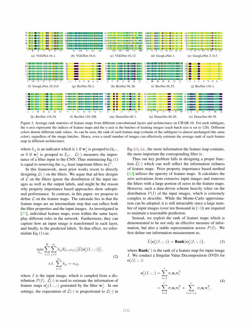
Figure 2. Average rank statistics of feature maps from different convolutional layers and architectures on CIFAR-10. For each subfigure,
the x-axis represents the indices of feature maps and the y-axis is the batches of training images (each batch size is set to 128). Different
colors denote different rank values. As can be seen, the rank of each feature map (column of the subfigure) is almost unchanged (the same
color), regardless of the image batches. Hence, even a small number of images can effectively estimate the average rank of each feature
map in different architectures.
where δij is an indicator which is 1 if wij is grouped to UCi ,
or 0 if wij is grouped to ICi . L(·) measures the impor-
tance of a filter input to the CNN. Thus minimizing Eq. (1)
is equal to removing the ni2 least important filters in Ci.
In this framework, most prior works resort to directly
designing L(·) on the filters. We argue that ad-hoc designs
of L on the filters ignore the distribution of the input im-
ages as well as the output labels, and might be the reason
why property importance based approaches show subopti-
mal performance. In contrast, in this paper, we propose to
define L on the feature maps. The rationale lies in that the
feature maps are an intermediate step that can reflect both
the filter properties and the input images. As investigated in
[37], individual feature maps, even within the same layer,
play different roles in the network. Furthermore, they can
capture how an input image is transformed in each layer,
and finally, to the predicted labels. To that effect, we refor-
mulate Eq. (1) as:
minδij
K∑
i=1
ni∑
j=1
δijEI∼P (I)
[
L(
oij(I, :, :)
)]
,
s.t.
ni∑
j=1
δij = ni2,
(2)
where I is the input image, which is sampled from a dis-
tribution P (I). L(·) is used to estimate the information of
feature maps oij(I, :, :) generated by the filter wi
j . In our
settings, the expectation of L(·) is proportional to L(·) in
Eq. (1), i.e., the more information the feature map contains,
the more important the corresponding filter is.
Thus our key problem falls in designing a proper func-
tion L(·) which can well reflect the information richness
of feature maps. Prior property importance based method
[14] utilizes the sparsity of feature maps. It calculates the
zero activations from extensive input images and removes
the filters with a large portion of zeros in the feature maps.
However, such a data-driven scheme heavily relies on the
distribution P (I) of the input images, which is extremely
complex to describe. While the Monte-Carlo approxima-
tion can be adopted, it is still intractable since a large num-
ber of input images (over ten thousand in [14]) are required
to maintain a reasonable prediction.
Instead, we exploit the rank of feature maps which is
demonstrated to be not only an effective measure of infor-
mation, but also a stable representation across P (I). We
first define our information measurement as:
L(
oij(I, :, :)
)
= Rank(
oij(I, :, :)
)
, (3)
where Rank(·) is the rank of a feature map for input image
I . We conduct a Singular Value Decomposition (SVD) for
oij(I, :, :):
oij(I, :, :) =
r∑
i=1
σiuivTi
=
r′∑
i=1
σiuivTi +
r∑
i=r′+1
σiuivTi ,
(4)
1532

where r = Rank(oij(I, :, :)) and r′ < r. δi, ui and vi are
the top-i singular values, left singular vector and right sin-
gular vector of oij(I, :, :), respectively. It can be seen that a
feature map with rank r can be decomposed into a lower-
rank feature map with rank r′, i.e.,∑r′
i=1 σiuivTi , and
some additional information, i.e.,∑r
i=r′+1 σiuivTi . Hence,
higher-rank feature maps actually contain more information
than lower-rank ones. Thus, the rank can serve as a reliable
measurement for information richness.
3.3. Tractability of Optimization
One critical point in the pruning procedures discussed
above falls in the calculation of ranks. However, it is pos-
sible that the rank of the feature maps oij ∈ R
g×hi×wi is
sensitive to the distribution of input images, P (I). For ex-
ample, the rank of oij(1, :, :) is not necessarily the same as
that of oij(2, :, :). To accurately estimate the expectation of
ranks, extensive input images have to be used, as with [14].
This poses a great challenge when evaluating the relative
importance of filters.
Fortunately, we empirically observe that the expectation
of ranks generated by a single filter is robust to the input im-
ages. To illustrate, we plot the average of rank values w.r.t.
different numbers of input batches in Fig. 2. It is obvious
that the colors (which indicate the values) of the average
ranks from a single filter are the same, which are irrespec-
tive to the image that CNNs receive. To explain, although
different images may have different ranks, the variance is
negligible. Hence, a small batch of input images can be
used to accurately estimate the expectation of the feature
map rank. Then, we define the rank expectation of feature
map oij as:
EI∼P (I)
[
L(
oij(I, :, :)
)]
≈
g∑
t=1
Rank(
oij(t, :, :)
)
. (5)
In our experiments, we set the number of images, g =500, to estimate the average rank, which is several orders of
magnitude smaller than [14], where over ten thousand input
images are used to estimate the sparsity of feature maps.
Besides, calculating the ranks of feature maps can be im-
plemented offline. Hence, Eq. (3) is easily tractable using
the above approximation. Combining Eq. (2) and Eq. (5),
we derive our final optimization objective as follows:
minδij
K∑
i=1
ni∑
j=1
δij(wij)
g∑
t=1
Rank(
oij(t, :, :)
)
,
s.t.
ni∑
j=1
δij = ni2.
(6)
It is intuitive that Eq. (6) can be minimized by pruning
the filters with ni2 least average ranks of feature maps.
Pruning Procedure. Given filters WCi in Ci and their
generated feature maps Oi, as defined in Sec. 3.1, we
prune WCi as follows: First, we calculate the average
rank of feature map oij in Oi, forming a rank set Ri =
{ri1, ri2, ..., r
ini} ∈ R
ni . Second, we re-rank the rank set in
decreasing order Ri = {riIi1
, riIi2
, ..., riIini
} ∈ Rni , where
Iij is the index of the j-th top value in Ri. Third, we
determine the values of ni1 (number of preserved filters)
and ni2 (number of pruned filters). Fourth, we obtain the
important filter set ICi = {wiIi1
,wiIi2
, ...,wiIini1
} where
the rank of wiIij
is riIij
. Similarly, we obtain the filter set
UCi = {wiUi
1
,wiUi
2
, ...,wiUi
ni2
}. Lastly, we remove the set
UCi and fine-tune the network with ICi as the initialization.
4. Experiments
4.1. Experimental Settings
Datasets and Baselines. To demonstrate our efficiency
in reducing model complexity, we conduct experiments on
both small and large datasets, i.e., CIFAR-10 [17] and Im-
ageNet [31]. We study the performance of different al-
gorithms on the mainstream CNN models, including VG-
GNet with a plain structure [32], GoogLeNet with an in-
ception module [33], ResNet with a residual block [11] and
DenseNet with a dense block [15]. Fig. 3 provides stan-
dards for pruning these popular networks. For all bench-
marks and architectures, we randomly sample 500 images
to estimate the average rank of each feature map.
Evaluation Protocols. We adopt the widely-used proto-
cols, i.e., number of parameters and required Float Points
Operations (denoted as FLOPs), to evaluate model size and
computational requirement. To evaluate the task-specific
capabilities, we provide top-1 accuracy of pruned models
and the pruning rate (denoted as PR) on CIFAR-10, and top-
1 and top-5 accuracies of pruned models on ImageNet.
Configurations. We use PyTorch [29] to implement the
proposed HRank approach. We solve the optimization prob-
lem by using Stochastic Gradient Descent algorithm (SGD)
with an initial learning rate of 0.01. The batch size, weight
decay and momentum are set to 128, 0.0005 and 0.9, re-
spectively. For each layer, we retrain the network for 30epochs after pruning2, with the learning rate being divided
by 10 at epochs 5 and 10 on CIFAR-10, and divided by
10 every 10 epochs on ImageNet. All experiments are con-
ducted on two NVIDIA GTX 1080Ti GPUs. It is worth not-
ing that for ResNet-50 on ImageNet, instead of fine-tuning
the network every time after pruning a convolution layer, we
prune the network in a per-block fashion, i.e. we fine-tune
the network only after performing pruning within the entire
2Better accuracy can be observed when training more epochs. How-
ever, it requires more training time.
1533
Nextlayer
Lastlayer
convolution
Lastlayer
maxpooling3x3
convolution1x1
convolution1x1
convolution1x1
convolution3x3
convolution3x3
convolution1x1
convolution3x3
concatenation
convolution1x1
convolution3x3
convolution1x1
(a)Plain structure
convolution3x3
convolution3x3
concatenation
(b)Inception module
(c)Residual block (d)Dense block
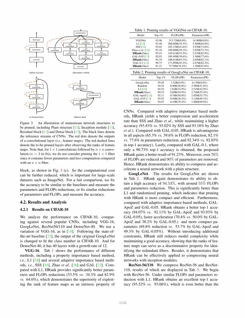
Figure 3. An illustration of mainstream network structures to
be pruned, including Plain structure [32], Inception module [33],
Residual block [11] and Dense block [15]. The black lines denote
the inference streams of CNNs. The red dots denote the outputs
of a convolutional layer (i.e., feature maps). The red dashed lines
denote the to-be-pruned layers after observing the ranks of feature
maps. Note that, for 1× 1 convolutions followed by n×n convo-
lution (n = 3 in (b)), we do not consider pruning the 1 × 1 filter
since it contains fewer parameters and less computation compared
with an n× n filter.
block, as shown in Fig. 3 (c). So the computational cost
can be further reduced, which is important for large-scale
datasets such as ImageNet. For a fair comparison, we fix
the accuracy to be similar to the baselines and measure the
parameters and FLOPs reductions, or fix similar reductions
of parameters and FLOPs, and measure the accuracy.
4.2. Results and Analysis
4.2.1 Results on CIFAR-10
We analyze the performance on CIFAR-10, compar-
ing against several popular CNNs, including VGG-16,
GoogLeNet, ResNet56/110 and DenseNet-40. We use a
variation of VGG-16, as in [18]. Following the state-of-
the-art baseline [23], the output of the original GoogLeNet
is changed to fit the class number in CIFAR-10. And for
DenseNet-40, it has 40 layers with a growth rate of 12.
VGG-16. Tab. 1 shows the performance of different
methods, including a property importance based method,
i.e., L1 [18] and several adaptive importance based meth-
ods, i.e., SSS [16], Zhao et al. [36] and GAL [23]. Com-
pared with L1, HRank provides significantly better param-
eters and FLOPs reductions (53.5% vs. 34.3% and 82.9%
vs. 64.0%), which demonstrates the superiority of exploit-
ing the rank of feature maps as an intrinsic property of
Table 1. Pruning results of VGGNet on CIFAR-10.
Model Top-1% FLOPs(PR) Parameters(PR)
VGGNet 93.96 313.73M(0.0%) 14.98M(0.0%)
L1 [18] 93.40 206.00M(34.3%) 5.40M(64.0%)
SSS [16] 93.02 183.13M(41.6%) 3.93M(73.8%)
Zhao et al. [36] 93.18 190.00M(39.1%) 3.92M(73.3%)
HRank(Ours) 93.43 145.61M(53.5%) 2.51M(82.9%)
GAL-0.05 [23] 92.03 189.49M(39.6%) 3.36M(77.6%)
HRank(Ours) 92.34 108.61M(65.3%) 2.64M(82.1%)
GAL-0.1 [23] 90.73 171.89M(45.2%) 2.67M(82.2%)
HRank(Ours) 91.23 73.70M(76.5%) 1.78M(92.0%)
Table 2. Pruning results of GoogLeNet on CIFAR-10.
Model Top-1% FLOPs(PR) Parameters(PR)
GoogLeNet 95.05 1.52B(0.0%) 6.15M(0.0%)
Random 94.54 0.96B(36.8%) 3.58M(41.8%)
L1 [18] 94.54 1.02B(32.9%) 3.51M(42.9%)
HRank(Ours) 94.53 0.69B(54.9%) 2.74M(55.4%)
GAL-ApoZ [14] 92.11 0.76B(50.0%) 2.85M(53.7%)
GAL-0.05 [23] 93.93 0.94B(38.2%) 3.12M(49.3%)
HRank(Ours) 94.07 0.45B(70.4%) 1.86M(69.8%)
CNNs. Compared with adaptive importance based meth-
ods, HRank yields a better compression and acceleration
rate than SSS and Zhao et al., while maintaining a higher
accuracy (93.43% vs. 93.02% by SSS and 93.18% by Zhao
et al.). Compared with GAL-0.05, HRank is advantageous
in all aspects (65.3% vs. 39.6% in FLOPs reduction, 82.1%
vs. 77.6% in parameters reduction, and 92.34% vs. 92.03%
in top-1 accuracy). Lastly, compared with GAL-0.1, where
only a 90.73% top-1 accuracy is obtained, the proposed
HRank gains a better result of 91.23%. Moreover, over 76%of FLOPs are reduced and 90% of parameters are removed.
Hence, HRank demonstrates its ability to compress and ac-
celerate a neural network with a plain structure.
GoogLeNet. The results for GoogLeNet are shown
in Tab. 2. HRank again demonstrates its ability to ob-
tain a high accuracy of 94.53%, with around 55% FLOPs
and parameters reduction. This is significantly better than
L1 and randomized pruning, which indicates that pruning
with HRank is more compact and efficient. Furthermore,
compared with adaptive importance based methods, GAL-
ApoZ and GAL-0.05, HRank obtains a better top-1 accu-
racy (94.07% vs. 92.11% by GAL-ApoZ and 93.93% by
GAL-0.05), faster acceleration (70.4% vs. 50.0% by GAL-
ApoZ and 38.2% by GAL-0.05.) and more compact pa-
rameters (69.8% reduction vs. 53.7% by GAL-ApoZ and
49.3% by GAL-0.05%). Without introducing additional
constraints, HRank still reduces model complexity while
maintaining a good accuracy, showing that the ranks of fea-
ture maps can serve as a discriminative property for iden-
tifying the redundant filters. Besides, it demonstrates that
HRank can be effectively applied to compressing neural
networks with inception modules.
ResNet-56/110. We compress ResNet-56 and ResNet-
110, results of which are displayed in Tab. 3. We begin
with ResNet-56. Under similar FLOPs and parameters re-
duction with L1, HRank obtains an excellent top-1 accu-
racy (93.52% vs. 93.06%), which is even better than the
1534
Table 3. Pruning results of ResNet-56/110 on CIFAR-10.
Model Top-1% FLOPs(PR) Parameters(PR)
ResNet-56 93.26 125.49M(0.0%) 0.85M(0.0%)
L1 [18] 93.06 90.90M(27.6%) 0.73M(14.1%)
HRank(Ours) 93.52 88.72M(29.3%) 0.71M(16.8%)
NISP [34] 93.01 81.00M(35.5%) 0.49M(42.4%)
GAL-0.6 92.98 78.30M(37.6%) 0.75M(11.8%)
HRank(Ours) 93.17 62.72M(50.0%) 0.49M(42.4%)
He et al. [13] 90.80 62.00M(50.6%) -
GAL-0.8 90.36 49.99M(60.2%) 0.29M(65.9%)
HRank(Ours) 90.72 32.52M(74.1%) 0.27M(68.1%)
ResNet-110 93.50 252.89M(0.0%) 1.72M(0.0%)
L1 [18] 93.30 155.00M(38.7%) 1.16M(32.6%)
HRank(Ours) 94.23 148.70M(41.2%) 1.04M(39.4%)
GAL-0.5 [23] 92.55 130.20M(48.5%) 0.95M(44.8%)
HRank(Ours) 93.36 105.70M(58.2%) 0.70M(59.2%)
HRank(Ours) 92.65 79.30M(68.6%) 0.53M(68.7%)
Table 4. Pruning results of DenseNet-40 on CIFAR-10.
Model Top-1% FLOPs(PR) Parameters(PR)
DenseNet-40 94.81 282.00M(0.0%) 1.04M(0.0%)
Liu et al.-40% [24] 94.81 190.00M(32.8%) 0.66M(36.5%)
GAL-0.01 [23] 94.29 182.92M(35.3%) 0.67M(35.6%)
HRank(Ours) 94.24 167.41M(40.8%) 0.66M(36.5%)
Zhao et al. [36] 93.16 156.00M(44.8%) 0.42M(59.7%)
GAL-0.05 [23] 93.53 128.11M(54.7%) 0.45M(56.7%)
HRank(Ours) 93.68 110.15M(61.0%) 0.48M(53.8%)
baseline model (93.52% vs. 93.26%). Besides, we observe
that HRank shares the same parameters reduction as NISP,
another property importance based method, but achieves a
better accuracy (93.17% vs. 93.01) and larger FLOPs reduc-
tion (50.0% vs. 35.5%). Moreover, HRank can effectively
deal with filters with more computation costs, leading to a
significant acceleration. Similar observations can be found
when compared with adaptive importance based methods,
including He et al. and GAL-0.8. HRank yields an impres-
sive acceleration (74.1% vs. 50.6% for He et al. and 60.2%
for GAL-0.8).
Next, we analyze the performance on ResNet-110. Sim-
ilar to what we have found with ResNet-56, HRank leads
to an improvement in accuracy over the baseline model
(94.23% vs. 93.50%) with around 41.2% FLOPs and 39.4%
parameters reduction. Besides, compared with L1, with a
slightly better complexity reduction, HRank again benefits
from better accuracy performance (94.23% vs. 93.30%).
Therefore, the rank can effectively reflect the relative im-
portance of a filter and serve as a better intrinsic property.
Finally, in comparison with GAL-0.5, HRank greatly re-
duces the model complexity (58.2% vs. 48.5% for FLOPs
and 59.2% vs. 44.8% for parameters) with only a small loss
in accuracy of 0.14%, while GAL-0.5 suffers a 0.95% accu-
racy drop. Moreover, we also maintain a similar accuracy
with GAL-0.5 (92.65% vs. 92.55%). Obviously, HRank
further accelerates the computation (68.6% vs. 48.5%) and
relieves the overload (68.7% vs. 44.8%). This indicates that
HRank is especially suitable for pruning neural networks
with residual blocks.
DenseNet-40. Tab. 4 summarizes the experimental re-
sults on DenseNet. We observe that HRank has the poten-
Table 5. Pruning results of ResNet-50 on ImageNet.
Model Top-1% Top-5% FLOPs Parameters
ResNet-50 [26] 76.15 92.87 4.09B 25.50M
SSS-32 [16] 74.18 91.91 2.82B 18.60M
He et al. [13] 72.30 90.80 2.73B -
GAL-0.5 [23] 71.95 90.94 2.33B 21.20M
HRank(Ours) 74.98 92.33 2.30B 16.15M
GDP-0.6 [22] 71.19 90.71 1.88B -
GDP-0.5 [22] 69.58 90.14 1.57B -
SSS-26 [16] 71.82 90.79 2.33B 15.60M
GAL-1 [23] 69.88 89.75 1.58B 14.67M
GAL-0.5-joint [23] 71.80 90.82 1.84B 19.31M
HRank(Ours) 71.98 91.01 1.55B 13.77M
ThiNet-50 [26] 68.42 88.30 1.10B 8.66M
GAL-1-joint [23] 69.31 89.12 1.11B 10.21M
HRank(Ours) 69.10 89.58 0.98B 8.27M
tial to remove more FLOPs. Though Liu et al. retains the
accuracy of the baseline, it produces only 32.8% FLOPs re-
ductions. In contrast, over 40.8% of FLOPs are removed by
HRank. Compared with Zhao et al. and GAL-0.05, HRank
achieves higher accuracy and FLOPs reduction, though it
removing fewer parameters. Overall, HRank has the poten-
tial to better accelerate neural networks. Hence, it can also
be applied in networks with dense blocks.
4.2.2 Results on ImageNet
We also conduct experiments for ResNet-50 on the chal-
lenging ImageNet dataset. The results are shown in Tab. 5.
Generally, HRank surpasses its counterparts in all aspects,
including top-1 and top-5 accuracies, as well as FLOPs
and parameters reduction. More specifically, 1.78× FLOPs
(2.30B vs. 4.09B for ResNet-50) and 1.58× parameters
(16.15M vs. 25.50M of ResNet-50) are removed by HRank,
while it still yields 74.98% top-1 accuracy and 92.33% top-
5 accuracy, significantly better than GAL-0.5. Moreover,
HRank obtains 71.98 top-1 accuracy and 91.01 top-5 ac-
curacy with 2.64× and 1.85× reductions of FLOPs and
parameters, respectively. Further, between ThiNet-50 and
GAL-1-joint, we observe that GAL-1-joint advances in bet-
ter accuracies, while ThiNet-50 shows more advantages in
FLOPs and parameters reductions. Nevertheless, HRank
outperforms both GAL-1-joint and ThiNet-50. Compared
with GAL-1-joint, which gains 69.31% top-1 and 89.12%
top-5 accuracies, HRank obtains 69.10% top-1 and 89.58%
top-5 accuracies. When comparing to ThiNet-50, bet-
ter complexity reductions are observed (0.98B FLOPs vs.
1.10B FLOPs for ThiNet-50 and 8.27M parameters vs.
8.66M for ThiNet-50). Hence, HRank also works well on
complex datasets.
4.3. Ablation Study
We conduct detailed ablation studies on variants of
HRank and keeping a portion of filters frozen during fine-
tuning. For brevity, we report the results of the ResNet-56
with top-1 accuracy of 93.17% in Tab. 3. Similar observa-
tions can be found in other networks and datasets.
1535

Figure 4. Top-1 accuracy for variants of HRank.
Variants of HRank. Three variants are proposed to
demonstrate the appropriateness of preserving filters with
high-rank feature maps, including: (1) Edge: Filters gener-
ating both low- and high-rank feature maps are pruned, (2)
Random: Filters are randomly pruned. (3) Reverse: Filters
generating high-rank feature maps are pruned. The pruning
rate is set to be the same as that with 93.17% top-1 accuracy
of HRank in Tab. 3. We report the corresponding top-1 ac-
curacy for each variant in Fig. 4. Among the variants, Edge
shows the best performance. To analyze, though part of fil-
ters with high-rank feature maps removed, it retains some
of those with relatively high-rank feature maps, which con-
tains rich information. Besides, HRank obviously outper-
forms its variants and Reverse performs the worst, demon-
strating that low-rank feature maps contain less information
and the corresponding filters can be safely removed.
Freezing Filters during Fine-tuning. We show that not
updating filters with higher-rank feature maps does little
damage to the model performance. To that effect, we show
the top-1 accuracy w.r.t. different rates of untrained weights
in Fig. 5. In Fig. 5(a), all the reserved filters are involved in
updating, which yields a top-1 accuracy of 93.17% (this can
be seen as the upper boundary for Fig. 5(b) and Fig. 5(c)). In
Fig. 5(b), around 15% - 20% of filters are untrained, which
returns a top-1 accuracy of 93.13%, which is only slightly
worse than the 93.17% of Fig. 5(a). The effect of a larger
percentage of untrained filters is displayed in Fig. 5(c), con-
sisting of around 20% - 25% of the overall weights. The
pruned model obtains a top-1 accuracy of 93.01%. Though
with a 0.11% drop in performance, it still outperforms the
methods compared in Fig. 3. Fig. 5 well supports our claim
that feature maps with high ranks contain more information.
5. Conclusions
In this paper, we present a novel filter pruning method
called HRank, which determines the relative importance of
filters by observing the rank of feature maps. To that ef-
fect, we empirically demonstrate that the average rank of
feature maps generated by a single filter are always the
same. Then, we mathematically prove that filters that gen-
(a) 0% of the filters are frozen, resulting in a top-1 precision of
93.17%.
(b) 15% - 20% of the filters are frozen, resulting in a top-1
precision of 93.13%.
(c) 20% - 25% of the filters are frozen, resulting in a top-1 pre-
cision of 93.01%.
Figure 5. How freezing filter weights during fine-tuning affects the
top-1 precision. The x-axes denote the indices of convolutional
layers. The blue, green and red denote the percentage of pruned,
trained and untrained filters, respectively.
erate lower-rank feature maps are less important and should
be removed first, and vice versa, which is also verified by
the experiments. In addition, we propose to freeze a portion
of the filters producing high-rank feature maps to further
reduce the fine-tuning cost, showing little compromise to
the model performance. Extensive experiments on various
modern CNNs demonstrate the effectiveness of HRank in
reducing the computational complexity and model size. In
the future work, we will do more on the theoretical analy-
sis on why the average rank of feature maps generated by a
single filter are always the same.
6. Acknowledge
This work is supported by the Nature Science Founda-
tion of China (No.U1705262, No.61772443, No.61572410,
No.61802324 and No.61702136), National Key R&D Pro-
gram (No.2017YFC0113000, and No.2016YFB1001503),
and Nature Science Foundation of Fujian Province, China
(No. 2017J01125 and No. 2018J01106).
1536

References
[1] Miguel A Carreira-Perpinan and Yerlan Idelbayev. Learning-
compression algorithms for neural net pruning. In Computer
Vision and Pattern Recognition (CVPR), 2018. 1
[2] Liang-Chieh Chen, George Papandreou, Iasonas Kokkinos,
Kevin Murphy, and Alan L Yuille. Deeplab: Semantic image
segmentation with deep convolutional nets, atrous convolu-
tion, and fully connected crfs. IEEE Transaction on Pattern
Analysis and Machine Learning (TPAMI), 2017. 1
[3] Wenlin Chen, James T. Wilson, Stephen Tyree, Killian
Q. Weinberger, and Yixin Chen. Compressing neural net-
works with the hashing trick. In International Conference
on Machine Learning (ICML), 2015. 1
[4] Jian Cheng, Pei-song Wang, Gang Li, Qing-hao Hu, and
Han-qing Lu. Recent advances in efficient computation of
deep convolutional neural networks. Frontiers of Informa-
tion Technology & Electronic Engineering (FITEE), 2018. 1
[5] Misha Denil, Babak Shakibi, Laurent Dinh, Marc’Aurelio
Ranzato, and Nando De Freitas. Predicting parameters in
deep learning. In Neural Information Processing Systems
(NeurIPS), 2013. 3
[6] Emily L Denton, Wojciech Zaremba, Joan Bruna, Yann Le-
Cun, and Rob Fergus. Exploiting linear structure within con-
volutional networks for efficient evaluation. In Neural Infor-
mation Processing Systems (NeurIPS), 2014. 1, 3
[7] Ross Girshick, Jeff Donahue, Trevor Darrell, and Jitendra
Malik. Rich feature hierarchies for accurate object detection
and semantic segmentation. In Computer Vision and Pattern
Recognition (CVPR), 2014. 1
[8] Song Han, Xingyu Liu, Huizi Mao, Jing Pu, Ardavan Pe-
dram, Mark A Horowitz, and William J Dally. Eie: efficient
inference engine on compressed deep neural network. In
International Conference on Computer Architecture (ISCA),
2016. 1
[9] Song Han, Huizi Mao, and William J Dally. Deep com-
pression: Compressing deep neural networks with pruning,
trained quantization and huffman coding. In International
Conference of Learning Representation (ICLR), 2015. 1
[10] Song Han, Jeff Pool, John Tran, and William J Dally. Learn-
ing both weights and connections for efficient neural net-
work. In Neural Information Processing Systems (NeurIPS),
2015. 1
[11] Kaiming He, Xiangyu Zhang, Shaoqing Ren, and Jian Sun.
Deep residual learning for image recognition. In Computer
Vision and Pattern Recognition (CVPR), 2016. 1, 2, 5, 6
[12] Yang He, Ping Liu, Ziwei Wang, Zhilan Hu, and Yi Yang.
Filter pruning via geometric median for deep convolutional
neural networks acceleration. In Computer Vision and Pat-
tern Recognition (CVPR), 2019. 2
[13] Yihui He, Xiangyu Zhang, and Jian Sun. Channel pruning
for accelerating very deep neural networks. In International
Conference on Computer Vision (ICCV), 2017. 2, 3, 7
[14] Hengyuan Hu, Rui Peng, Yu-Wing Tai, and Chi-Keung
Tang. Network trimming: A data-driven neuron pruning ap-
proach towards efficient deep architectures. arXiv preprint
arXiv:1607.03250, 2016. 2, 3, 4, 5, 6
[15] Gao Huang, Zhuang Liu, Laurens Van Der Maaten, and Kil-
ian Q Weinberger. Densely connected convolutional net-
works. In Computer Vision and Pattern Recognition (CVPR),
2017. 2, 5, 6
[16] Zehao Huang and Naiyan Wang. Data-driven sparse struc-
ture selection for deep neural networks. In European Con-
ference on Computer Vision (ECCV), 2018. 2, 3, 6, 7
[17] Alex Krizhevsky, Geoffrey Hinton, et al. Learning multiple
layers of features from tiny images. Technical report, Cite-
seer, 2009. 2, 5
[18] Hao Li, Asim Kadav, Igor Durdanovic, Hanan Samet, and
Hans Peter Graf. Pruning filters for efficient convnets. In In-
ternational Conference of Learning Representation (ICLR),
2017. 1, 2, 3, 6, 7
[19] Mingbao Lin, Rongrong Ji, Shaojie Li, Qixiang Ye,
Yonghong Tian, Jianzhuang Liu, and Qi Tian. Filter sketch
for network pruning. arXiv preprint arXiv:2001.08514,
2020. 1
[20] Mingbao Lin, Rongrong Ji, Yuxin Zhang, Baochang Zhang,
Yongjian Wu, and Yonghong Tian. Channel pruning via au-
tomatic structure search. arXiv preprint arXiv:2001.08565,
2020. 1
[21] Shaohui Lin, Rongrong Ji, Chao Chen, Dacheng Tao, and
Jiebo Luo. Holistic cnn compression via low-rank decompo-
sition with knowledge transfer. IEEE Transaction on Pattern
Analysis and Machine Learning (TPAMI), 2018. 3
[22] Shaohui Lin, Rongrong Ji, Yuchao Li, Yongjian Wu, Feiyue
Huang, and Baochang Zhang. Accelerating convolutional
networks via global & dynamic filter pruning. In Interna-
tional Joint Conference on Artificial Intelligence (IJCAI),
2018. 7
[23] Shaohui Lin, Rongrong Ji, Chenqian Yan, Baochang Zhang,
Liujuan Cao, Qixiang Ye, Feiyue Huang, and David Doer-
mann. Towards optimal structured cnn pruning via gener-
ative adversarial learning. In Computer Vision and Pattern
Recognition (CVPR), 2019. 2, 3, 6, 7
[24] Zhuang Liu, Jianguo Li, Zhiqiang Shen, Gao Huang,
Shoumeng Yan, and Changshui Zhang. Learning efficient
convolutional networks through network slimming. In Inter-
national Conference on Computer Vision (ICCV), 2017. 2,
3, 7
[25] Jonathan Long, Evan Shelhamer, and Trevor Darrell. Fully
convolutional networks for semantic segmentation. In Com-
puter Vision and Pattern Recognition (CVPR), 2015. 1
[26] Jian-Hao Luo, Jianxin Wu, and Weiyao Lin. Thinet: A filter
level pruning method for deep neural network compression.
In Computer Vision and Pattern Recognition (CVPR), 2017.
2, 3, 7
[27] Pavlo Molchanov, Stephen Tyree, Tero Karras, Timo Aila,
and Jan Kautz. Pruning convolutional neural networks for
resource efficient inference. In International Conference of
Learning Representation (ICLR), 2016. 2, 3
[28] Jongsoo Park, Sheng Li, Wei Wen, Ping Tak Peter Tang, Hai
Li, Yiran Chen, and Pradeep Dubey. Faster cnns with di-
rect sparse convolutions and guided pruning. In International
Conference of Learning Representation (ICLR), 2016. 1
1537
[29] Adam Paszke, Sam Gross, Soumith Chintala, Gregory
Chanan, Edward Yang, Zachary DeVito, Zeming Lin, Al-
ban Desmaison, Luca Antiga, and Adam Lerer. Automatic
differentiation in pytorch. In Neural Information Processing
Systems (NeurIPS), 2017. 5
[30] Shaoqing Ren, Kaiming He, Ross Girshick, and Jian Sun.
Faster r-cnn: Towards real-time object detection with region
proposal networks. In Neural Information Processing Sys-
tems (NeurIPS), 2015. 1
[31] Olga Russakovsky, Jia Deng, Hao Su, Jonathan Krause, San-
jeev Satheesh, Sean Ma, Zhiheng Huang, Andrej Karpathy,
Aditya Khosla, Michael Bernstein, et al. Imagenet large
scale visual recognition challenge. Internation Journal of
Computer Vision (IJCV), 2015. 2, 5
[32] Karen Simonyan and Andrew Zisserman. Very deep convo-
lutional networks for large-scale image recognition. arXiv
preprint, 2014. 2, 5, 6
[33] Christian Szegedy, Wei Liu, Yangqing Jia, Pierre Sermanet,
Scott Reed, Dragomir Anguelov, Dumitru Erhan, Vincent
Vanhoucke, and Andrew Rabinovich. Going deeper with
convolutions. In Computer Vision and Pattern Recognition
(CVPR), 2015. 1, 2, 5, 6
[34] Ruichi Yu, Ang Li, Chun-Fu Chen, Jui-Hsin Lai, Vlad I
Morariu, Xintong Han, Mingfei Gao, Ching-Yung Lin, and
Larry S Davis. Nisp: Pruning networks using neuron im-
portance score propagation. In Computer Vision and Pattern
Recognition (CVPR), 2018. 2, 3, 7
[35] Xiangyu Zhang, Jianhua Zou, Xiang Ming, Kaiming He, and
Jian Sun. Efficient and accurate approximations of nonlin-
ear convolutional networks. In Computer Vision and Pattern
Recognition (CVPR), 2015. 3
[36] Chenglong Zhao, Bingbing Ni, Jian Zhang, Qiwei Zhao,
Wenjun Zhang, and Qi Tian. Variational convolutional neural
network pruning. In Computer Vision and Pattern Recogni-
tion (CVPR), 2019. 2, 3, 6, 7
[37] Bolei Zhou, Yiyou Sun, David Bau, and Antonio Torralba.
Revisiting the importance of individual units in cnns via ab-
lation. arXiv preprint arXiv:1806.02891, 2018. 4
1538