arX

iv:1

409.

3748

v1 [

mat

h.PR

] 1

2 Se

p 20

14

The phase transitions of the planar random-cluster and Potts

models with q ≥ 1 are sharp

Hugo Duminil-Copin and Ioan Manolescu

September 9, 2018

Abstract

We prove that random-cluster models with q ≥ 1 on a variety of planar lattices have a

sharp phase transition, that is that there exists some parameter pc below which the model

exhibits exponential decay and above which there exists a.s. an infinite cluster. The result

may be extended to the Potts model via the Edwards-Sokal coupling.

Our method is based on sharp threshold techniques and certain symmetries of the lattice;

in particular it makes no use of self-duality. Part of the argument is not restricted to planar

models and may be of some interest for the understanding of random-cluster and Potts

models in higher dimensions.

Due to its nature, this strategy could be useful in studying other planar models satisfying

the FKG lattice condition and some additional differential inequalities.

1 Introduction

Main statement. The random-cluster model (or FK percolation) was introduced by Fortuinand Kasteleyn in 1969 as a class of models satisfying specific series and parallel laws. It is relatedto many other models, including the q-state Potts models (q = 2 being the particular case ofthe Ising model). In addition to this, the random-cluster model exhibits a variety of interestingfeatures, many of which are still not fully understood.

Consider a finite graph G = (VG,EG). The random-cluster measure with edge-weight p ∈[0,1] and cluster-weight q > 0 on G is a measure φp,q,G on configurations ω ∈ 0,1EG . An edgeis said to be open (in ω) if ω(e) = 1, otherwise it is closed. The configuration ω can be seen asa subgraph of G with vertex set VG and edge-set e ∈ EG ∶ ω(e) = 1. A cluster is a connectedcomponent of ω. Let o(ω), c(ω) and k(ω) denote the number of open edges, closed edges andclusters in ω respectively. The probability of a configuration is then equal to

φp,q,G(ω) = po(ω)(1 − p)c(ω)qk(ω)Z(p, q,G) ,

where Z(p, q,G) is a normalizing constant called the partition function.Consider a connected planar locally-finite doubly periodic graph G , i.e. a graph which is

invariant under the action of some lattice Λ ≃ Z ⊕ Z. The model can be extended to G bytaking limits of measures on finite graphs Gn tending to G (with certain boundary conditions,see Section 2.2 for details). We call such limits infinite-volume measures. As discussed later, forany pair of parameters p ∈ [0,1] and q ≥ 1, at least one infinite-volume measure exists, but it isnot necessarily unique. For q ≥ 1, the infinite-volume model exhibits a phase transition at somecritical parameter pc(q) (depending on the lattice). The aim of the present paper is to give aproof of the sharpness of this phase transition.

Theorem 1.1. Fix q ≥ 1. Let G be a planar locally-finite doubly periodic connected graphinvariant under reflection with respect to the line (0, y), y ∈ R and rotation by some angleθ ∈ (0, π) around 0. There exists pc = pc(G ) ∈ [0,1] such that

1

• for p < pc, there exists c = c(p,G ) > 0 such that for any x, y ∈ G ,

φp,q[x and y are connected by a path of open edges] ≤ exp(−c∣x − y∣), (1.1)

• for p > pc, there exists a.s. an infinite open cluster under φp,q,where φp,q is the unique infinite-volume random-cluster measure on G with edge-weight p andcluster-weight q.

Remark 1.2. The fact that, for p ≠ pc, there exists a unique infinite-volume measure withedge-weight p may easily be shown by adapting [14, Thm. 6.17].

The sharpness of the phase transition was proved in arbitrary dimension for percolation in[1, 17] and for the Ising model in [2]. For planar random-cluster models with arbitrary cluster-weight q ≥ 1, the sharpness had been previously derived only in the case of the square, triangularand hexagonal lattices, see [3]. A similar result is proved for so-called isoradial graphs in [9].It may be worth mentioning that, contrary to the present work, [3] and [9] are both based onintegrability properties of the model.

The exponential decay of the two-point function is key to the study of the subcritical phase.It implies properties such as exponential decay of the cluster-size, finite susceptibility, Ornstein-Zernike estimates and mixing properties, to mention but a few. We do not go into details here,but rather refer the reader to the monographs [13, 14] for further reading.

Our method is based on the sharp threshold property and on certain symmetries of thelattice. A corollary of our results is that self-dual models are critical.

Corollary 1.3. The critical parameters pc(q) of the square, triangular and hexagonal latticessatisfy

on the square lattice: pc(q) =√q/(1 +√q),on the triangular lattice: pc(q) is the unique solution p in [0,1] of p3 + 3p2(1 − p) = q(1 − p)3,on the hexagonal lattice: pc(q) is the unique solution p in [0,1] of p3 − 3qp(1 − p)2 = q2(1 − p)3.

The model on the square lattice with the above parameter is indeed self-dual; the ones on thetriangular and hexagonal lattices are not per se. They are dual to each other, but also relatedthrough the star–triangle transformation (see [14, Sec. 6.6]).

As mentioned above, the previous corollary was obtained in [3]. Nevertheless, the presentmethod has the advantage of using self-duality for the identification of the critical point only, andnot for the proof of sharpness (in [3], the self-duality is used in the proof of a Russo-Seymour-Welsh type estimate leading to the sharpness of the phase transition).

Extensions of Theorem 1.1 We discuss several (potential) generalisations of the previoustheorem.

First, the biperiodic graph G = (VG ,EG ) may be replaced by a weighted biperiodic graph(G , J), where J is a family of strictly positive weights on edges. For any subgraph G = (VG,EG)of G and β ≥ 0, we define

φβ,q,G,J(ω) = (∏e∈EG(eβJe − 1)ω(e)) ⋅ qk(ω)Z(β, q,G,J) , (1.2)

where Z(β, q,G,J) is a normalizing constant. One may easily see that in the case of Je = Jfor any e ∈ EG, we obtain the previous definition with p = 1 − e−Jβ. As before, infinite-volumemeasures may be defined on G by taking limits.

Theorem 1.4. Fix q ≥ 1. Let G be a planar locally-finite doubly periodic connected weightedgraph invariant under reflection with respect to the line (0, y), y ∈ R and rotation by someangle θ ∈ (0, π) around 0. There exists βc = βc(G , J) ≥ 0 such that

2

• for β < βc, there exists c = c(β,G , J) > 0 such that for any x, y ∈ G ,

φβ,q,J[x and y are connected by a path of open edges] ≤ exp(−c∣x − y∣),• for β > βc, there exists a.s. an infinite open cluster under φβ,q,J ,

where φβ,q,J is the unique infinite-volume random-cluster measure on G with parameters q andβ.

The proof of this theorem follows exactly the same lines as the one of Theorem 1.1 exceptthat the notation becomes heavier. Thus we will only focus on Theorem 1.1.

A second potential extension is to planar random-cluster models with finite range interac-tions. Consider a planar graph G = (VG ,EG ) with the properties of Theorem 1.1. For someR ≥ 1 define a modified graph G = (VG ,EG

), with same vertex set as G but with (u, v) ∈ EG

if

the graph distance between u and v in G is less than or equal to R. (For R = 1, G = G .)We believe that our methods may be modified to prove Theorem 1.1 (and its inhomogeneous

version Theorem 1.4) for G . In particular we expect that Theorem 1.1 also applies to therandom-cluster model on slabs, i.e. on the graphs of the form G × 0, . . . ,Rd with d,R ≥ 1. Wediscuss this further in a forthcoming article.

A final potential extension is to models other than the random-cluster model. Our argumentsare somewhat generic, and one can try to use them for models similar to those studied here.More precisely, to obtain our result, we only need the model to satisfy the conditions listed inSection 6. We discuss this point further in Section 6, when the appropriate notation is in place.

Consequences for the Potts model. Fix some finite weighted graph (G,J), where J =(Je)e∈EGis a family of positive real numbers. Also fix a set of parameters β ≥ 0 and q ∈ N with

q ≥ 2. The Potts model on G with q states and inverse temperature β is a probability measureµβ,q,G,J on 1, . . . , qVG , for which the weight of a configuration σ is given by

µβ,q,G,J(σ) = e−βHq,G,J (σ)

ZPotts

β,q,G,J

,

whereHq,G,J(σ) = − ∑

e=(x,y)∈EG

Je1σx=σy

and ZPotts

β,q,G,J is a normalizing constant. The sum in the second equation is taken over all un-ordered pairs of neighbours x, y.

A well-known coupling (sometimes called the Edwards-Sokal coupling) links the Potts andrandom-cluster models. We only briefly describe how to obtain the former from the latter. Fordetails see [14, Thm 4.91].

Choose a random-cluster configuration ω according to φβ,q,G,J , where φβ,q,G,J is definedas in (1.2). Assign to each cluster of ω a state (or colour) chosen uniformly in 1, . . . , q,independently for different clusters. This generates a random configuration σ ∈ 1, . . . , qVG .(Note the two sources of randomness used in generating σ: the randomness in the choice of ωand that in the colouring of the clusters of ω.) Then σ follows the Potts measure µβ,q,G,J .

Consider now a planar locally-finite doubly periodic weighted graph (G , J). As for therandom-cluster, infinite-volume Potts measures may be defined. The phase transition in thiscase is decided by the existence of long-range correlations. In particular, if βc is the criticalparameter, then

• for β < βc, there exists a unique infinite-volume measure (long-range correlations vanish),• for β > βc, there exist multiple infinite-volume measures (long-range correlations exist).

3

It follows trivially from the above coupling that

µβ,q,G,J(σx = σy) = 1

q+q − 1

qφβ,q,G,J(x and y are connected by a path of open edges),

hence the phase transition of the Potts model can be linked to that of the associated random-cluster model. In particular, when Je = J for all e ∈ EG , βc(q) = − 1

Jlog(1 − pc(q)).

Our main result may be translated as follows.

Theorem 1.5. Fix q ≥ 2. Let G be a planar locally-finite doubly periodic connected weightedgraph invariant under reflection with respect to the line (0, y), y ∈ R and rotation by someangle θ ∈ (0, π) around 0. There exists βc = βc(G , J) ≥ 0 such that,

• for β < βc, there exists a unique infinite-volume Potts measure µβ,q,J with parameters βand q on (G , J). Moreover there exists c = c(β,G ) > 0 such that for any x, y ∈ G ,

µβ,q,J[σx = σy] − 1

q≤ exp(−c∣x − y∣),

• for β > βc, there exist multiple infinite-volume Potts measures with parameters β and q

on (G , J).Strategy of the proof. Let φ0p,q be the infinite-volume measure on G with free boundaryconditions (see the next section for a precise definition). It is obtained as the limit of random-cluster measures φp,q,Gn on finite subgraphs Gn of G that tend increasingly to G . Define

pc ∶= inf p ∈ (0,1) ∶ φ0p,q(x is connected by a path of open edges to infinity) > 0pc ∶= supp ∈ (0,1) ∶ lim

n→∞−

1nlog [φ0p,q(0 and ∂Λn are connected by a path of open edges)] > 0.

Note that pc ≤ pc. We wish to prove that pc = pc (this is simply another way of stating themain result), and we therefore focus on the inequality pc ≥ pc. The proof of the latter is basedon the study of probabilities of crossing rectangles. For the sake of simplicity, let us restrictour attention in this introduction to rectangles of width 2n and height n, i.e. translates of[0,2n]× [0, n]. A rectangle is crossed horizontally (vertically) if it contains a path of open edgesgoing from its left side to its right side (respectively from the bottom side to the top side). Thestrategy follows three main steps:

Step 1. We first prove that for any p > pc, the probability of crossing vertically (i.e. in the “easydirection”) a rectangle of size 2n × n is bounded away from 0 uniformly in n.

We show this by proving that for any 0 < ε < p, if the φ0p,q-probability of crossing vertically arectangle of size 2n×n drops below a certain benchmark (even for a single value of n), thenthe φp−ε,q,G -probability that two points are connected by an open path decays exponentiallyfast (see Proposition 3.1 for the precise statement). A similar (but stronger) statementwas proved by Kesten for percolation [16]. He proved that, given a percolation measure,if the probability of crossing the rectangle vertically is too small, then exponential decayfollows for that measure. The difference with our result is that, in the case of percolation,one does not need to alter the parameter of the measure (see Remark 1.6 for more details).

We highlight the fact that this part of the proof is not specific to the planar case.

Step 2. Using the first step, we show that for any p > pc, the probability of crossing horizontally(i.e. in the “hard direction”) a rectangle of size 2n × n is bounded away from 0 uniformlyin n.

This step is the most difficult. It corresponds to proving a “Russo-Seymour-Welsh” (RSW)type result: if crossing probabilities in the easy direction are bounded away from 0, then it

4

is the same in the hard direction. Such results were first proved in the context of Bernoullipercolation on the square lattice [18, 19]. Similar statements have been recently obtainedfor the Ising model [8, 5] and the random-cluster models with cluster-weight 1 ≤ q ≤ 4 [11],but only for the square lattice. These results usually represent the first step towards adeep understanding on the critical phase.

In the present paper we prove a weaker statement than these RSW results: we show that,if crossing probabilities in the easy direction are bounded away from 0 for some edge-weight p, then it is the same in the hard direction for any p′ > p. As in the first step, thedifference with previous results is that we need to increase the edge-weight to obtain thedesired conclusion.

Step 3. We show that if p < p′ < pc are such that the φ0p,q-probability of crossing horizontally a

rectangle of size 2n × n is bounded away from 0 uniformly in n, then the φ0p′,q-probabilityof these events tends to 1 as n tends to ∞.

This step is based on an argument from [12] that combines an influence theorem and acoupling argument to obtain a sharp threshold inequality (see Corollary 5.2).

Observe that these steps combine together to give the proof of the theorem. Indeed supposepc < pc and take pc < p0 < p1 < p2 < pc. By steps 1 and 2, the probabilities under φ0p0,q of crossingin the hard direction rectangles of size 2n × n are bounded away from 0, uniformly in n. Bystep 3 these crossing probabilities tend to 1 under φ0p1,q. As a consequence the probability of adual crossing in the easy direction of a 2n by n rectangle tends to 0. But step 1 also applies todual measures, hence, for the edge-weight p2, the two-point function of the dual model decaysexponentially fast. This implies via a classical argument that there exists an infinite-cluster inthe primal model, and this is a contradiction.

Remark 1.6. The proofs of Steps 1 and 2 require varying the edge-weight p. Nevertheless, weexpect that this is not indispensable. Bernoulli percolation is an example for which the proofsof Steps 1 and 2 are valid without changing p, but the known proofs of this fact rely heavilyon independence. In order to tackle more general models (in particular those having long-rangedependence), we employ the differential inequality (2.6) invoking the Hamming distance, whichentails altering p. The related differential inequality (2.5) is used in Step 3. Exploiting them totheir full strength is the main novelty of this article.

Open questions. We end this introduction by mentioning three related open questions.The first is to investigate to which other models the methods of this paper may be adapted.

We discuss this in Section 6, where we identify specific conditions for such models.The second is to obtain results similar to Theorem 1.1 for lattices in dimensions d > 2. We

believe that some of the techniques presented in this article can be harnessed in more generaldimensions (we think in particular of Step 1 and inequalities (2.5) and (2.6)). Nevertheless, themethods of Steps 2 and 3 are based on certain features of planarity, and we are currently unableto extend Theorem 1.1 to higher dimension.

Finally we mention a broader direction of research. Just as the method of [3], our articleprovides very little information on the critical phase of the random-cluster model. Recent results(for instance [11, 20, 6, 7]) have illustrated that it is possible extract knowledge of the criticalphase of random-cluster models from the theory of discrete holomorphic observables. But thistheory is often based on integrability properties of the model, properties which are not truefor general random-cluster models on planar locally-finite doubly periodic graphs. Therefore, itis very challenging to understand how to extend our knowledge of the critical random-clustermodel on the square lattice to more general settings. A first step towards this goal is to provethat the results of Steps 1 and 2 are valid without changing the edge-parameter.

5

Organisation of the paper. Section 2 is dedicated to defining the model and explaining theproperties needed in the proof of Theorem 1.1. The next sections follow the steps describedabove: in Sections 3 and 4 we prove two finite size criteria for exponential decay (correspondingto Steps 1 and 2) that we then use in Section 5 to prove our main theorem (this corresponds toStep 3). In Section 6 we investigate a possible extension of the result to more general models.

2 Notations and basic facts on the model

2.1 Graph definitions

The lattice G . Fix for the rest of the paper a locally-finite planar connected graph G =(VG ,EG ) embedded in the plane R2 (in such a way that edges are straight lines intersecting at

their end-points only) and assume there exist u and v ∈ R2 non collinear, and θ ∈ (0, π) suchthat the following maps are graphs automorphisms of the embedded graph G :

• the translations by vectors u and v,• the rotation of angle θ around 0,• the orthogonal reflection with respect to the vertical line (0, y), y ∈ R.

It may be seen that, since G is required to be locally finite, there are only two possible values forθ, namely π

3and π

2. The triangular lattice is an example corresponding to the first case, while

the square lattice corresponds to the second (obviously, other examples may be given in bothcases). For simplicity, we will only treat the case θ = π

2in the following; the results also hold

in the case θ = π3, with some standard adjustments of the proofs. It may be shown that, if we

allow some rescaling, we may consider the lattice to be invariant by• the translations by (1,0) and (0,1),• rotation by π

2around the origin,

• the orthogonal symmetry with respect to the vertical line (0, y), y ∈ R.In the rest of this article, the graph G will be referred to as the lattice. Two vertices x and y ofVG are said to be neighbours if (x, y) ∈ EG . We then write x ∼ y.

The graph G = (VG,EG) will always denote a finite subgraph of G , i.e. EG is a finite subsetof EG and VG is the set of end-points of EG. We denote by ∂G the boundary of G, i.e.

∂G = x ∈ VG ∶ ∃y ∉ VG with x ∼ y.For a < b and c < d, let R = [a, b] × [c, d] be the subgraph of G induced by the vertices of VG

in [a, b] × [c, d]. This type of graph will be called a rectangle. For n ≥ 0, let Λn = [−n,n]2.Dual lattice and dual graphs. Let G

∗ be the dual lattice of G , obtained by placing a vertexin each face of G and joining two vertices of G

∗ if the corresponding faces of G are adjacent. Notethat G ∗ enjoys the same symmetries as G . For e ∈ EG , set e∗ for the edge of G ∗ intersecting e.For a finite graph G, define G∗ to be the graph with edge-set EG∗ ∶= e∗, e ∈ EG, and vertex-setVG∗ given by the end-points of edges in EG∗ .

The space of configurations. Let G = (VG,EG) be a subgraph of G . We will always workwith elements ω of Ω = 0,1EG , called configurations. Edges e with ω(e) = 1 are called open(in ω), while others are closed (in ω). As mentioned above, ω can be seen as a subgraph of Gwhose vertex-set is VG and edge-set is e ∈ EG ∶ ω(e) = 1.

A path on G is a sequence of vertices u0, . . . , un ∈ VG with (ui, ui+1) ∈ EG for i = 0, . . . , n − 1.It is called open if (ui, ui+1) is open in ω for every i. Two vertices a and b are said to be connected(in ω on G), if there exists an open path connecting them. The event that a and b are connected

is denoted by aω,G←Ð→ b (or simply a

G←→ b or even a←→ b when no confusion is possible). Two sets A

and B are connected (denoted A ←→ B) if there exists a pair of connected vertices (a, b) ∈ A×B.A maximal set of connected vertices is called a cluster.

6

When G = [a, b] × [c, d] is a rectangle and A = a × [c, d] and B = b × [c, d] (respectively

A = [a, b] × c and B = [a, b] × d), the event Aω,G←Ð→ B is also denoted Ch([a, b] × [c, d])

(respectively Cv([a, b]×[c, d])) and if it occurs we say that G is crossed horizontally (respectivelyvertically). An open path from A to B is called a horizontal crossing (respectively verticalcrossing). When a = 0 and c = 0, we simply write Ch(b, d) and Cv(b, d) for the events above.When b − a > d − c, horizontal crossings are called crossings in the hard direction, while verticalones are crossings in the easy direction. The terms are exchanged when b − a < d − c.

To each configuration ω ∈ Ω is associated a dual configuration ω∗ on G∗ defined by ω∗(e∗) =1 − ω(e). A dual-path on G∗ is a sequence of vertices u0, . . . , un ∈ VG∗ with (ui, ui+1) ∈ EG∗ fori = 0, . . . , n − 1. It is called dual-open if ω∗(ui, ui+1) = 1 for all i. Two dual-vertices u and v are

said to be dual-connected (written uω∗,G∗

←ÐÐ→ v or simply u∗←→ v when no confusion is possible) if

there is a dual-open path connecting them. A maximal set of connected dual-vertices is calleda dual-cluster. The definitions of crossings extend to dual configurations in the obvious way.

2.2 Basic properties of the random-cluster model

For more details and proofs we direct the reader to [14] or [7].

Boundary conditions. Let G = (VG,EG) be a finite subgraph of G . A boundary condition ξ

is a partition of ∂G. We denote by ωξ the graph obtained from the configuration ω by identifying(or wiring) the vertices in ∂G that belong to the same element of the partition ξ. Boundaryconditions should be understood as encoding how vertices are connected outside G. The prob-ability measure φξ

p,q,Gof the random-cluster model on G with parameters p ∈ [0,1], q ≥ 0 and

boundary condition ξ is defined on Ω by

φξp,q,G(ω) ∶= po(ω)(1 − p)c(ω)qk(ω

ξ)

Zξ(p, q,G) , (2.1)

where Zξ(p, q,G) is a normalizing constant referred to as the partition function. Above, o(ω),c(ω) and k(ωξ) correspond to the number of open and closed edges of ω, and the number ofclusters of ωξ.

Two specific boundary conditions are particularly important. The free boundary condition,denoted 0, correspond to the partition composed of singletons only (no wiring between boundaryvertices). The wired boundary condition, denoted 1, correspond to the partition ∂G (allvertices are wired together). In addition to these two, we will sometimes consider boundaryconditions induced by a configuration ξ outside G: two vertices are wired together if there existsa path between them in ξ. We will identify ξ with the induced boundary condition and simplywrite φξp,q,G for the corresponding measure.

Domain Markov property. Let G ⊂ F be two finite subgraphs of G . A configuration ω on Fmay be viewed as a configuration on G by taking its restriction ω∣G to edges of G. The restrictionof the configuration ω to edges of F ∖G induces boundary conditions on G as explained below.The domain Markov property states that for any p, q, any boundary condition ξ on F and anyψ ∈ 0,1EF ∖EG ,

φξp,q,F(ω∣G = ⋅ ∣ω(e) = ψ(e), e ∈ EF ∖EG) = φψξ

p,q,G(⋅), (2.2)

where ψξ is the partition induced by the equivalence relation xRy if x and y are connected inψξ.

The domain Markov property implies the following finite-energy property. For any ε > 0,the conditional probability for an edge to be open, knowing the states of all the other edges,is bounded away from 0 and 1 uniformly in p ∈ [ε,1 − ε] and in the state of other edges. This

7

property extends to finite sets of edges (with a constant which gets worse and worse as thecardinality of the set increases).

Stochastic ordering for q ≥ 1. For any G, the set 0,1EG has a natural partial order. Anevent A is increasing if for any ω ≤ ω′, ω ∈ A implies ω′ ∈ A. The random-cluster model satisfiesthe following properties:

1. (FKG inequality) Fix p ∈ [0,1], q ≥ 1 and some boundary condition ξ. Let A and B twoincreasing events, then φξp,q,G(A ∩B) ≥ φξp,q,G(A)φξp,q,G(B).

2. (comparison between boundary conditions) Fix p ∈ [0,1], q ≥ 1 and ξ and ψ two boundaryconditions. Assume that ξ ≤ ψ, meaning that the partition ψ is coarser than ξ (there aremore wirings in ψ than in ξ), then for any increasing event A, φξ

p,q,G(A) ≤ φψ

p,q,G(A).

3. (comparison between different edge parameters) Fix p1 ≤ p2, q ≥ 1 and some boundarycondition ξ. Then for any increasing event A, φξp1,q,G(A) ≤ φξp2,q,G(A).

Infinite-volume measures for q ≥ 1. We will consider measures on infinite-volume configu-rations, i.e. on 0,1EG . Recall that for any finite subgraph G of G , a configuration ω ∈ 0,1EG

induces a boundary condition on G that we will exceptionally write in this paragraph χ(ω).Under χ(ω), two vertices x, y ∈ ∂G are wired if and only if they are connected in ω on G ∖G.An infinite-volume random-cluster measure on G with parameters p and q is a measure φp,q on0,1EG with the property that, for all finite subgraphs G of G ,

φp,q(ω∣G = ⋅ ∣χ(ω) = ξ) = φξp,q,G(⋅), (2.3)

for all boundary conditions ξ for which the conditioning is not degenerate.The properties of the previous paragraph extend to infinite-volume measures by (2.3).One may prove that for any pair of parameters (p, q), there exists at least one such measure.

When q ≥ 1, one may for instance take the limit of measures with wired (resp. free) boundaryconditions on Λn. The measure obtained in the limit is called the infinite-volume measure withwired (resp. free) boundary conditions and is denoted by φ1p,q (resp. φ0p,q).

In general there is no reason that, for a given pair of parameters (p, q), there is a uniqueinfinite-volume measure. Nevertheless, for q ≥ 1, the set Dq of values of p for which there existat least two distinct infinite-volume measures is at most countable, see [14, Theorem (4.60)].This property can be combined with the stochastic ordering between different edge-weights toshow the existence of a critical point pc ∈ [0,1] such that:

• for any infinite-volume measure with p < pc, there is almost surely no infinite cluster,• for any infinite-volume measure with p > pc, there is almost surely an infinite cluster.

When the planar, locally finite, doubly-periodic graph is non-degenerate, pc can be proved tobe different from 0 and 1 using a variant of the classical Peierls argument.

While the above is true also for lattices in higher dimensions, for planar lattices such as G

an additional argument shows that Dq ⊆ pc (in fact in any dimension one has Dq ⊆ [pc,1], see[14, Theorem 5.16]). See the discussion following Remark 2.1 for details.

Planar duality. Let G be a finite graph and ξ ∈ 0,1EG ∖EG . If ω is distributed accordingto φξ

p,q,G, the configuration ω∗ is also distributed as a random-cluster configuration on G∗ with

different parameters. More precisely, we find that

φξp,q,G(ω) = φξ∗

p∗,q∗,G∗(ω∗),

wherepp∗

(1 − p)(1 − p∗) = q and q∗ = q

8

and ξ∗ is the boundary condition on ∂G∗ induced by the dual-configuration ξ∗ ∈ 0,1EG ∗∖EG∗ .For instance, dual measures extend to the whole of G

∗ and, if ω follows φ1p,q,G (respectively

φ0p,q,G ), then ω∗ is distributed as φ0p∗,q,G ∗ (respectively φ1p∗,q,G ∗).

Remark 2.1. As a consequence of Theorem 1.1, for q ≥ 1 and p > pc, there exists c = c(p, q) > 0such that

φp,q(u ∗←→ v) ≤ exp(−c∣u − v∣), for all u, v ∈ VG ∗ . (2.4)

Indeed, an adaptation of Zhang’s argument (as that of [14, Thm 6.17]) shows that, for anyvalues of q ≥ 1 and p ∉ Dq, it is impossible to have with positive probability infinite clusters inboth ω and ω∗. Thus, if p > pc, there is no infinite cluster in ω∗, and Theorem 1.1 applied tothe dual random-cluster model implies (2.4).

Differential inequalities. The two following theorems are essential to our study. The first isa direct adaptation of the more general statement of Graham and Grimmett [12, Thm. 5.3].

Theorem 2.2 ([12]). For any q ≥ 1 there exists a constant c > 0 such that, for any p ∈ (0,1),any finite graph G, any boundary condition ξ and any increasing event A,

d

dpφξp,q,G(A) ≥ cφξ

p,q,G(A)(1 − φξ

p,q,G(A)) log ( 1

2mA,p

) , (2.5)

where mA,p =maxe∈EG(φξp,q,G(A ∣ω(e) = 1) − φξp,q,G(A ∣ω(e) = 0)).

The original result concerns a more general class of measures than that of the random-clustermodel, hence the slightly more complicated statement of [12, Thm. 5.3]. The above formulationis easily deduced using an explicit bound for the finite energy property of the random-clustermodel:

p

q≤ φξp,q,G(ω(e) = 1 ∣ω(f), f ≠ e) ≤ p, for all G,e, ξ, p and q ≥ 1.

In order to state the second result, we introduce the notion of Hamming distance. For anevent A and a configuration ω, define HA(ω) as the graph distance in the hypercube 0,1EG

(or Hamming distance) between ω and the set A. When A is increasing, it corresponds to theminimal number of edges that need to be turned to open in order to go from ω to A. Thefollowing may be found in [14, Thm. 2.53] or [15].

Theorem 2.3 ([15]). For any q ≥ 1, any p ∈ (0,1), any finite graph G and boundary conditionξ, we have that for any increasing event A,

d

dplog(φξ

p,q,G(A)) ≥ φ

ξp,q,G(HA)

p(1 − p) . (2.6)

In the above φξp,q,G(HA) is the expectation of HA under φξ

p,q,G.

Remark 2.4. In this article (2.6) will be used in its integrated form. Consider two values p′ < pand an increasing event A. Since HA is a decreasing function, by integrating (2.6) between p′

and p we find

φξp′,q,G(A) ≤ φξp,q,G(A) exp [ − 4(p − p′)φξp,q,G(HA)]. (2.7)

Now, consider an event A depending on a finite set of edges E and assume that the infinite-volume measures at p′ and p are unique. By taking ξ = 1 and taking the limit in (2.7) as G tendsto G (both sides of the inequality converge) we obtain

φp′,q(A) ≤ φp,q(A) exp [ − 4(p − p′)φp,q(HA)]. (2.8)

9

From now on, we fix q ≥ 1 and G . For ease, we drop them from the notation. We

will frequently work with infinite-volume measures for different values of p and will

always assume that these values are not in Dq. In such case, φp means the unique

infinite-volume measure with parameter p.

Remark 2.5. Since Dq is countable, the different claims could be easily extended to values of pin Dq by density (φp simply denotes any infinite-volume measure in this case). Also note thatwe are mainly interested in p < pc for which p ∉ Dq anyway (we prefer to state the claims in fullgenerality since they may be of some use in other contexts).

3 Crossings in the easy direction

The goal of this section is to prove the following result, which corresponds to Step 1.

Proposition 3.1. If p0 ∈ (0,1) is such that there exists an infinite-volume measure φp0 with

lim infn→∞

φp0(Cv(2n,n)) = 0,then for any p < p0 there exists c = c(p) > 0 such that for any x, y ∈ G

φp(x ←→ y) ≤ exp(−c∣x − y∣).Remark 3.2. This proposition can be proved in any dimension d ≥ 2. The claim should beadapted as follows: if the liminf of probabilities of crossing sets of the form [0,2n]d−1 × [0, n]from [0,2n]d−1 × 0 to [0,2n]d−1 × n is equal to 0 for some edge-weight p0, then there isexponential decay for any p < p0 (i.e. (1.1) holds for p < p0).

The proof of the proposition is based on the following two lemmas. Let Cx be the cluster ofthe site x. For simplicity we will henceforth assume 0 ∈ VG .

Lemma 3.3. Let p0 > 0. If there exists an infinite-volume measure φp0 and κ > 0 such thatφp0(∣C0∣4+κ) <∞, then for any p < p0, there exists c = c(p) > 0 such that for any n ≥ 0,

φp(0 ←→ ∂Λn) ≤ exp(−cn). (3.1)

It is easy to see that (3.1) is equivalent to exponential decay, as defined in (1.1). The previouslemma is classical, see [15] or [14, Thm. 5.64]. We only mention that its proof is based on thedifferential inequality (2.6).

Lemma 3.4. Let p > p′. For any N ≥ n,

φp′(Cv(2N,N)) ≤ exp [−(p − p′)Nn (1 − φp(Cv(2n,n)))2N/n] .

Proof Consider the event Cv(2N,n). Any vertical open crossing of [0,2N]× [0, n] contains atleast one of the following:

• a vertical crossing of a rectangle [kn, (k + 2)n] × [0, n], for some 0 ≤ k < ⌊N/n⌋,• a horizontal crossing of a square [kn, (k + 1)n] × [0, n], for some 0 ≤ k < ⌊N/n⌋.

All the events above have probability bounded from below by φp(Cv(2n,n)). Using the FKGinequality for the complements of these events, we obtain

1 − φp(Cv(2N,n)) ≥ (1 − φp(Cv(2n,n)))2N/n. (3.2)

As a consequence, we deduce that

φp(HCv(2N,n)) ≥ φp(HCv(2N,n) ≥ 1) = 1 − φp(Cv(2N,n)) ≥ (1 − φp(Cv(2n,n)))2N/n.10

Since Cv(2N,N) is included in the intersection of ⌊Nn⌋ translates of Cv(2N,n), it follows that

φp (HCv(2N,N)) ≥ ⌊Nn ⌋(1 − φp(Cv(2n,n)))2N/n.By (2.8) for p′ < p we find the result (we have ignored the integer parts in the lemma since

1p(1−p)⌊N/n⌋ ≥ N/n). ◻

The idea of the proof of Proposition 3.1 goes as follows. Assuming that φp(Cv(2n,n)) is smallfor some n, we apply Lemma 3.4 repeatedly, and obtain a bound on the decay of φp−ε(Cv(2N,N))as N increases. A bound on the moments of ∣C0∣ follows.

Proof of Proposition 3.1 Fix some ε > 0 and p0 > ε. Let α > 2 be a (large) constant, wewill see later how to choose it. (We prefer not to give an explicit value for α now, though therequirements for it are universal.) Consider a small constant δ0 > 0, we will see in the proof howto choose δ0 (its value only depends on α and ε). Assume that there exists a positive integer n0such that φp0(Cv(2n0, n0)) ≤ δα0 and define recursively, for k ≥ 0,

δk+1 = δ2k,

nk+1 = nk/δ2k,pk+1 = pk − δk.

Assuming δ0 is sufficiently small, the inequality φpk(Cv(2nk, nk)) ≤ δαk and Lemma 3.4 imply

φpk+1(Cv(2nk+1, nk+1)) ≤ exp (−(pk − pk+1)nk+1nk(1 − φpk(Cv(2nk, nk)))2nk+1/nk)

≤ exp ( − (1 − δαk )2δ−2

k

δk) ≤ δ2αk = δαk+1.

Further assume that δ0 is chosen small enough that limk→∞ pk ≥ p0 − ε. We deduce that for anyk ≥ 0,

φp0−ε(Cv(2nk, nk)) ≤ δαk . (3.3)

Let us extend the previous bound to values of N different from the nk ∶ k ≥ 0. For nk ≤ N <nk+1, by (3.2) or by a simple union bound,

φp0−ε(Cv(2N,N)) ≤ φp0−ε(Cv(2N,nk)) ≤ 2nk+1

nkδαk ≤ 2(n0N )

α−24

.

In the last inequality we have used that δi = δ1/2k−i

kfor any i ≤ k, and therefore

δ4k ≤k

∏i=0

δ2i =n0

nk+1≤n0

N.

It easily follows that φp0−ε(0 ↔ ∂ΛN) ≤ 8(n0

N)α−24 for any N . Since a cluster of cardinality

larger than N has diameter at least a constant times√N , we find easily that φp−ε(∣C0∣5) < ∞

provided that α is chosen large enough (α > 42 suffices). By Lemma 3.3, the above implies thatfor any p < p0 − ε, there exists c = c(p) > 0 such that for any n ≥ 0,

φp(0 ←→ ∂Λn) ≤ exp(−cn).Now, if lim inf φp0(Cv(2n,n)) = 0, then for any ε > 0, there exists n0 such that φp0(Cv(2n0, n0)) ≤δα0 , where α and δ0 = δ0(ε,α) are chosen as above. By the argument above φp exhibits exponentialdecay for any p < p0. ◻

11

4 Crossing probabilities in the hard direction

The object of this section is the following result.

Proposition 4.1. If p ∈ (0,1) is such that there exists an infinite-volume measure φp with

lim infn→∞

φp(Cv(2n,n)) > 0, (4.1)

then for any p0 > p,

lim infn→∞

φp0(Ch(2n,n)) > 0.In light of Proposition 3.1, the above result has the following immediate corollary, which is

exactly the claim mentioned in Step 2 of the introduction.

Corollary 4.2. If p0 ∈ (0,1) is such that there exists an infinite-volume measure φp0 with

lim infn→∞

φp0(Ch(2n,n)) = 0,then for any p < p0 there exists c = c(p) > 0 such that for any n ≥ 0,

φp(0 ←→ ∂Λn) ≤ e−cn.The proof of Proposition 4.1 is based on the following lemma and its corollary. Some termi-

nology is needed for their statement. Let γ1, . . . , γK be open paths in some rectangle [a, b]×[c, d].We say they are separated in [a, b]×[c, d] if they are contained in distinct clusters of [a, b]×[c, d](beware of the fact that we are speaking of clusters in [a, b]× [c, d]). In other words, no two areconnected by open paths inside [a, b] × [c, d].Lemma 4.3. Let p ∈ (0,1) and n ∈ N. There exist universal constants c0, c1 > 0 such that, if1 ≤ I ≤ n/400 is an integer that satisfies

I2 ≤ c0φp(Cv(2n,n))

φp(Ch(2n,n))c1/I , (4.2)

then

φp ([0,2n] × [0, n/2] has 2I separated vertical crossings) ≥ 12φp(Cv(2n,n)). (4.3)

The statement above may seem cryptic. Here are a few observations that may help thereader assimilate the lemma. First of all, the conclusion (4.3) is strongest when I is large, butthe hypothesis (4.2) is effectively an upper bound on I. Moreover it may even be that thereexists no I with the properties required in the lemma. The lemma will be applied in situationswhere φp(Cv(2n,n)) is bounded below by some constant. Then it states that, if φp(Ch(2n,n)) isclose to 0 (so that I may be large and satisfy (4.2)), the rectangle [0,2n]×[0, n/2] contains manyseparated vertical crossings with positive probability. Furthermore, the smaller φp(Ch(2n,n)),the larger the number of separated vertical crossings.

In words, this statement asserts that if typically [0,2n] × [0, n] is crossed vertically, but theprobability of crossings in the hard direction is very small, then any vertical crossing needs totwist substantially, creating many separated crossings of a slightly smaller (in height) rectangle(see the discussion preceding the proof of Lemma 4.3).

The proof of Lemma 4.3 represents the major difficulty of this article. We postpone it to theend of the section and first explain how it implies Proposition 4.1. A key observation is that theexistence of separated vertical crossings of [0,2n]×[0, n/2] (as in (4.3)) implies a lower bound onthe Hamming distance to the event Ch(2n,n). Using (2.6), this yields an explicit lower boundon crossing probabilities in the hard direction. We formalize this next.

12

For x ∈ (0,1), set

f(x) ∶= ⎧⎪⎪⎨⎪⎪⎩log(1/x)

log log(1/x) if x < 1/e−∞ otherwise

.

Corollary 4.4. Let δ > 0. There exist constants c2 = c2(δ) > 0 and c3 = c3(δ) > 0 such that forany p > p′ and n with φp(Cv(2n,n)) ≥ δ and n ≥ c2f[φp(Ch(2n,n))], the following holds:

φp′(Ch(n,n/2)) ≤ exp [ − c3(p − p′)δ exp (c3f[φp(Ch(2n,n))])].Proof Fix δ > 0 and p > p′. Let n be an integer such that φp(Cv(2n,n)) ≥ δ and n ≥c2f[φp(Ch(2n,n))], for a constant c2 specified later. Define I = ⌊cff[φp(Ch(2n,n))]⌋, wherecf = cf(δ) is some large constant to be specified. It is easy then to see that, for this choice of I,we have

I2 ≤ c0φp(Cv(2n,n))

φp(Ch(2n,n))c1/Ifor every n ≥ 1, provided that cf is large enough (where c0, c1 are the universal constants ofLemma 4.3). Furthermore, we find that I ≤ n/400 by setting c2 = 400cf . Finally, we may limitourselves to the case where φp (Ch(2n,n)) is small enough to have I ≥ 1 (the constant c3 maybe chosen so that the conclusion holds trivially otherwise).

The previous paragraph shows that with these choices of cf and c2, I satisfies the assumptionsof Lemma 4.3, and we find

φp ([0,2n] × [0, n/2] contains 2I separated vertical crossings) ≥ 1

2φp(Cv(2n,n)) ≥ δ

2.

Since the crossings in (4.3) are separated, there exist also at least 2I − 1 ≥ 2I−1 disjoint dualvertical crossings of [0,2n] × [0, n/2]. This generates a lower bound on the expected Hammingdistance to the event Ch(2n,n/2):

φp (HCh(2n,n/2)) ≥ 2I ⋅ δ4 . (4.4)

Inequality (2.8) (the integrated form of (2.6)) implies that

φp′(Ch(2n,n/2)) ≤ φp(Ch(2n,n/2)) exp ( − 1

p(1 − p) ⋅ (p − p′) ⋅ 2I ⋅ δ4)≤ exp [ − (p − p′)δ exp (c3f[φp(Ch(2n,n))])],

where the constant c3 > 0 depends on cf and therefore on δ only. In the last inequality, we usedthe choice of I proposed at the very beginning of the proof. Finally, by combining crossings inthe hard direction of five rectangles with side lengths n and n/2, we may obtain a crossing of[0,2n] × [0, n/2]. Thus,

φp′ (Ch(n,n/2))5 ≤ φp′ (Ch(2n,n/2)) ,and the result follows. ◻

Let us now prove Proposition 4.1 using Corollary 4.4.

13

Proof of Proposition 4.1 Fix p0 > p and assume that infn≥0

φp(Cv(2n,n)) = δ > 0. Let c2, c3

be the constants given by Corollary 4.4 for δ given above. For integers n0 and 0 ≤ k ≤ log2√n0,

define

nk = 2−kn0,

pk = p0 − (p0 − p) k

∑i=1

2−i,

βk = φpk(Ch(2nk, nk)).We aim to apply Corollary 4.4 with the above values of n and p. We start by a simple verificationof the hypothesis.

Claim. For n0 large enough and for any integer 0 ≤ k ≤ log2√n0,

nk > c2f(βk).Proof of the Claim. Assume that there exists an integer 0 ≤ k ≤ log2

√n0 such that nk ≤ c2f(βk).

We have

φp(Ch(2nk, nk)) ≤ φpk(Ch(2nk, nk)) = βk ≤ exp ( − nkc2 ) ≤ n−10k , (4.5)

where the second inequality uses that f(x) ≤ log(1/x). In the last inequality we have supposedthat nk is larger than some rank depending only on c2. We may assume this since nk ≥

√n0 and

we may take n0 as large as we wish.Consider x ∈ 0 × [0, nk] and y ∈ 1

2nk × [0, nk] maximizing (among such pairs of vertices)

the probability that they are connected in [0, 12nk] × [0, nk]. Then

φp (x [0,nk/2]×[0,nk]←ÐÐÐÐÐÐÐ→ y) ≥ 1

n2k

φp (Ch(12nk, nk)) .Combining four times the above (also using reflection symmetry) we obtain

φp(Ch(2nk, nk)) ≥ 1

n8k

φp(Ch(12nk, nk))4.Confronting this to (4.5) implies

φp (Ch(12nk, nk)) ≤ n−1/2k≤ n−1/40 .

But φp (Ch(12nk, nk)) ≥ δ by assumption and symmetry under π2-rotation. This leads to a

contradiction for n0 large enough.

The argument that (4.5) contradicts φp (Ch(12nk, nk)) ≥ δ will be used several times in therest of the paper.

We now fix n0 large, in particular large enough for the property of the claim to be satisfied.Then we may apply Corollary 4.4 to each triplet (nk, pk, pk+1) to obtain

βk+1 ≤ exp ( − c32−(k+1)(p0 − p)δ exp (c3f(βk))).Hence, there exist constants ∆ ≥ e40 and c∆ > 0, depending on p0 − p, c3 and δ only, such thatif we assume βk ≤ c∆∆−k, the previous displayed equation implies that

c3f(βk) ≥ 2k log 2 and βk+1 ≤ exp [ − c3(p0 − p)δ exp (c32f(βk))] ≤ βk

∆≤ c∆∆−(k+1).

14

Assume now that β0 ≤ c∆. Then, by the above, βk ≤ c∆∆−k for any k ≤ log2√n0. Therefore,

there exists m ∈ [√n0, n0] (m = n⌊log2√n0⌋) such that

φp (Ch(2m,m)) ≤ c∆e−40⌊log2√n0⌋ ≤ c∆m−10.

Using the same procedure as at the end of the proof of the previous claim we obtain a contra-diction for n0 large enough, since m ≥

√n0 and φp (Ch(2m,m)) ≥ δ by definition.

Therefore, the assumption φp0(Ch(2n0, n0)) = β0 ≤ c∆ can not hold for n0 large enough. Thisimplies that

lim infn→∞

φp0(Ch(2n,n)) ≥ c∆ > 0.◻

We now turn to the core of the argument, namely the proof of Lemma 4.3. The proof isinspired by the work of Bollobás and Riordan on Bernoulli percolation on Voronoi tessellations[4] (even though it makes use of different ingredients, and that the claim is not the same). Westart with a brief description.

Fix I as in Lemma 4.3 and let v = 1100I

. First we obtain an upper bound, as a functionof φp(Ch(2n,n)), for the probability of crossing horizontally rectangles of height k and width(1 + v)k for k ∈ [n

4, n]. Using this bound, we show that one vertical crossing of [0,2n]×[0, n] con-

tains, with high probability, three crossings of the slightly thinner rectangle [0,2n]× [23vn, (1−23v)n]. Repeating the procedure, we finally obtain 2I crossings of [0,2n] × [n

4, 3n

4]. Moreover,

these crossings are separated by dual paths. See Figure 4.

Proof of Lemma 4.3 Fix p,n and I satisfying the assumptions of the lemma and set v = 1100I

(we will specify the values of the universal constants c0 and c1 later in the proof). Define

α = supφp(Ch(⌈(2 + v)k⌉,2k)) ∶ k ∈ [n8 , n2 ]. (4.6)

For any k ∈ [n8, n2], we may combine 32/v crossings in the hard direction of rectangles with

sides of length 2k and ⌈(2 + v)k⌉ (both horizontal and vertical) to create a horizontal crossingof [0,2n] × [0, n]. Choosing k ∈ [n

8, n2] achieving the maximum in (4.6), we conclude that

α ≤ φp(Ch(2n,n))v/32 ≤ φp(Ch(2n,n))2c1/I , (4.7)

by setting c1 = 1/6400.We start by proving a series of claims that will then be used to prove the lemma. For these

claims, fix an integer k ∈ [n4, n2] and u ∈ [v,1/3] such that ku ∈ Z. The first three claims are

concerned with crossings of the rectangle R(k) = [−(1 + u)k, (1 + u)k] × [0,2k].Claim 1. Let E (k) be the event that there exists a vertical open crossing of R(k), with thelower endpoint not contained in [−3uk,3uk] × 0, or the higher endpoint not contained in[−3uk,3uk] × 2k. Then

φp(E (k)) ≤ 4(α +√α).Proof of Claim 1. Let β be the φp-probability that there exists a vertical open crossing of R(k),with the lower endpoint in [−(1 + u)k,−3uk] × 0.

The probability of crossing [−(1+u)k, (1−2u)k]×[0,2k] vertically is at most α (by definitionof α). Thus, with probability β −α, there exists a vertical crossing of R(k) with an endpoint in[−(1 + u)k,−3uk] × 0 which intersects the vertical line (1 − 2u)k × [0,2k]. See Figure 1. Byreflection with respect to −3uk × [0,2k], with probability β − α, there exists an open path in[−(1 + 4u)k, (1 − 5u)k] × [0,2k], between [−3uk, (1 − 5u)k] × 0 and −(1 + 4u)k × [0,2k].

When combining the two events above using the FKG inequality, we obtain that, withprobability at least (β −α)2, there exists a horizontal open crossing of [−(1 + 4u)k, (1 − 2u)k] ×[0,2k]. This event has probability less than α, hence β ≤ α +

√α. By considering the other

possibilities for the lower and higher endpoints, the claim follows.

15

(1− 2u)k

(2 + 2u)k

(1− 2u)k

O

3uk

2k

γ1

γ2

3uk

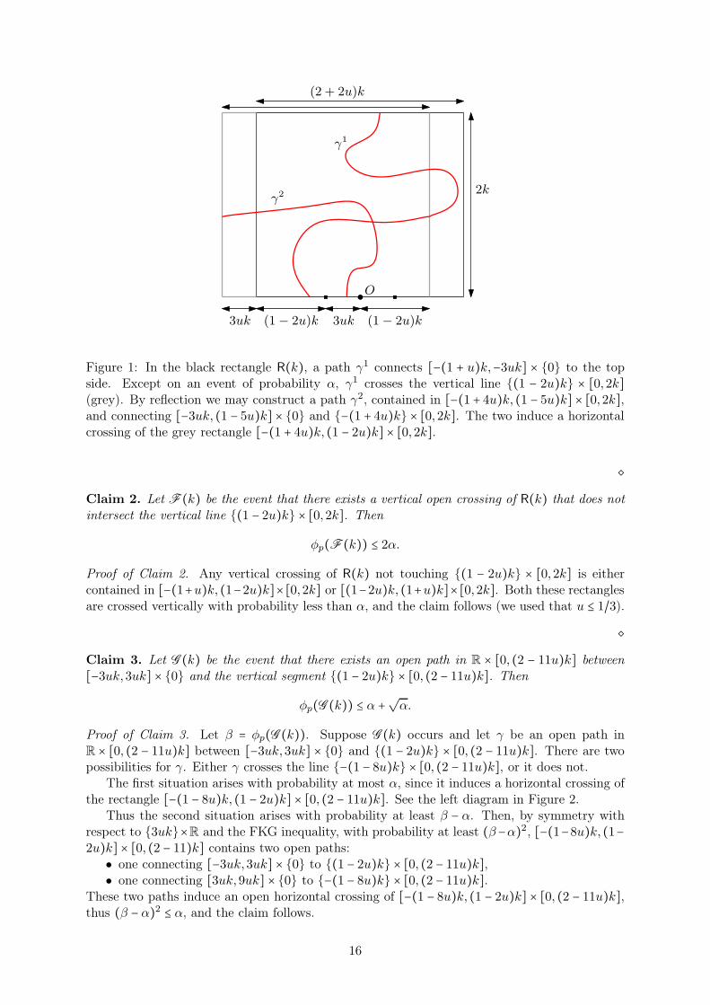
Figure 1: In the black rectangle R(k), a path γ1 connects [−(1 + u)k,−3uk] × 0 to the topside. Except on an event of probability α, γ1 crosses the vertical line (1 − 2u)k × [0,2k](grey). By reflection we may construct a path γ2, contained in [−(1 + 4u)k, (1 − 5u)k] × [0,2k],and connecting [−3uk, (1 − 5u)k] × 0 and −(1 + 4u)k × [0,2k]. The two induce a horizontalcrossing of the grey rectangle [−(1 + 4u)k, (1 − 2u)k] × [0,2k].

Claim 2. Let F(k) be the event that there exists a vertical open crossing of R(k) that does notintersect the vertical line (1 − 2u)k × [0,2k]. Then

φp(F(k)) ≤ 2α.Proof of Claim 2. Any vertical crossing of R(k) not touching (1 − 2u)k × [0,2k] is eithercontained in [−(1+u)k, (1−2u)k]×[0,2k] or [(1−2u)k, (1+u)k]×[0,2k]. Both these rectanglesare crossed vertically with probability less than α, and the claim follows (we used that u ≤ 1/3).

Claim 3. Let G (k) be the event that there exists an open path in R × [0, (2 − 11u)k] between[−3uk,3uk] × 0 and the vertical segment (1 − 2u)k × [0, (2 − 11u)k]. Then

φp(G (k)) ≤ α +√α.Proof of Claim 3. Let β = φp(G (k)). Suppose G (k) occurs and let γ be an open path inR × [0, (2 − 11u)k] between [−3uk,3uk] × 0 and (1 − 2u)k × [0, (2 − 11u)k]. There are twopossibilities for γ. Either γ crosses the line −(1 − 8u)k × [0, (2 − 11u)k], or it does not.

The first situation arises with probability at most α, since it induces a horizontal crossing ofthe rectangle [−(1 − 8u)k, (1 − 2u)k] × [0, (2 − 11u)k]. See the left diagram in Figure 2.

Thus the second situation arises with probability at least β − α. Then, by symmetry withrespect to 3uk×R and the FKG inequality, with probability at least (β−α)2, [−(1−8u)k, (1−2u)k] × [0, (2 − 11)k] contains two open paths:

• one connecting [−3uk,3uk] × 0 to (1 − 2u)k × [0, (2 − 11u)k],• one connecting [3uk,9uk] × 0 to −(1 − 8u)k × [0, (2 − 11u)k].

These two paths induce an open horizontal crossing of [−(1 − 8u)k, (1 − 2u)k] × [0, (2 − 11u)k],thus (β − α)2 ≤ α, and the claim follows.

16

(1− 2u)k(1− 8u)k

(2−11

u)k

6uk

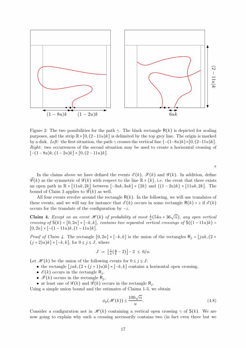
Figure 2: The two possibilities for the path γ. The black rectangle R(k) is depicted for scalingpurposes, and the strip R×[0, (2−11u)k] is delimited by the top grey line. The origin is markedby a disk. Left: the first situation, the path γ crosses the vertical line −(1−8u)k×[0, (2−11u)k].Right: two occurrences of the second situation may be used to create a horizontal crossing of[−(1 − 8u)k, (1 − 2u)k] × [0, (2 − 11u)k].

In the claims above we have defined the events E (k), F(k) and G (k). In addition, defineG (k) as the symmetric of G (k) with respect to the line R× k, i.e. the event that there existsan open path in R × [11uk,2k] between [−3uk,3uk] × 2k and (1 − 2u)k × [11uk,2k]. Thebound of Claim 3 applies to G (k) as well.

All four events revolve around the rectangle R(k). In the following, we will use translates ofthese events, and we will say for instance that E (k) occurs in some rectangle R(k) + z if E (k)occurs for the translate of the configuration by −z.

Claim 4. Except on an event H (k) of probability at most 1u(54α + 36√α), any open vertical

crossing of S(k) = [0,2n] × [−k, k], contains two separated vertical crossings of S((1 − 11u)k) =[0,2n] × [−(1 − 11u)k, (1 − 11u)k].Proof of Claim 4. The rectangle [0,2n] × [−k, k] is the union of the rectangles Rj = [juk, (2 +(j + 2)u)k] × [−k, k], for 0 ≤ j ≤ J , where

J ∶= ⌊ 1u(nk− 2)⌋ − 2 ≤ 6/u.

Let H (k) be the union of the following events for 0 ≤ j ≤ J :• the rectangle [juk, (2 + (j + 1)u)k] × [−k, k] contains a horizontal open crossing,• E (k) occurs in the rectangle Rj ,• F(k) occurs in the rectangle Rj ,• at least one of G (k) and G (k) occurs in the rectangle Rj .

Using a simple union bound and the estimates of Claims 1-3, we obtain

φp(H (k)) ≤ 100√α

u. (4.8)

Consider a configuration not in H (k) containing a vertical open crossing γ of S(k). We arenow going to explain why such a crossing necessarily contains two (in fact even three but we

17

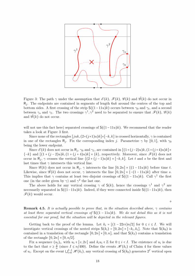
γ1

γ2

γt

γs

Figure 3: The path γ under the assumption that E (k), F(k), G (k) and G (k) do not occur inRj. The endpoints are contained in segments of length 6uk around the centres of the top andbottom sides. A first crossing of the strip S((1− 11u)k) occurs between γ0 and γt, and a secondbetween γs and γ1. The two crossings γ1, γ2 need to be separated to ensure that F(k), G (k)and G (k) do not occur.

will not use this fact here) separated crossings of S((1−11u)k). We recommend that the readertakes a look at Figure 3 first.

Since none of the rectangles [juk, (2+(j+1)u)k]×[−k, k] is crossed horizontally, γ is containedin one of the rectangles Rj. Fix the corresponding index j. Parametrize γ by [0,1], with γ0being the lower endpoint.

Since E (k) does not occur in Rj, γ0 and γ1, are contained in [(1+(j−2)u)k, (1+(j+4)u)k]×−k and [(1 + (j − 2)u)k, (1 + (j + 4)u)k] × k, respectively. Moreover, since F(k) does notoccur in Rj , γ crosses the vertical line (2 + (j − 1)u)k × [−k, k]. Let t and s be the first andlast times that γ intersects this vertical line.

Since G (k) does not occur in Rj, γ intersects the line [0,2n] × (1 − 11u)k before time t.Likewise, since G (k) does not occur, γ intersects the line [0,2n] × −(1 − 11u)k after time s.This implies that γ contains at least two disjoint crossings of S((1 − 11u)k). Call γ1 the firstone (in the order given by γ) and γ2 the last one.

The above holds for any vertical crossing γ of S(k), hence the crossings γ1 and γ2 arenecessarily separated in S((1−11u)k). Indeed, if they were connected inside S((1−11u)k), thenF(k) would occur.

Remark 4.5. It is actually possible to prove that, in the situation described above, γ containsat least three separated vertical crossings of S((1 − 11u)k). We do not detail this as it is notessential for our proof, but the situation will be depicted in the relevant figures.

Getting back to the proof of the lemma. Let ki = ⌊(1 − 22vi)n/2⌋ for 0 ≤ i ≤ I. We willinvestigate vertical crossings of the nested strips S(ki) = [0,2n] × [−ki, ki]. Note that S(k0) iscontained in a translation of the rectangle [0,2n] × [0, n], and that S(kI) contains a translationof the rectangle [0,2n] × [0, n/2].

Fix a sequence (ui)i, with ui ∈ [v,2v] and kiui ∈ Z for 0 ≤ i < I. The existence of ui is dueto the fact that v ≥ 4

n(since I ≤ n/400). Define the events H (ki) of Claim 4 for these values

of ui. Except on the event ⋃I−1i=0 H (ki), any vertical crossing of S(k0) generates 2I vertical open

18

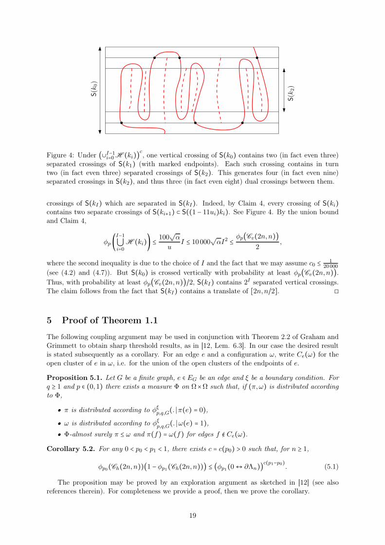
S(k

0)

S(k

2)

Figure 4: Under (∪I−1i=0 H (ki))c, one vertical crossing of S(k0) contains two (in fact even three)separated crossings of S(k1) (with marked endpoints). Each such crossing contains in turntwo (in fact even three) separated crossings of S(k2). This generates four (in fact even nine)separated crossings in S(k2), and thus three (in fact even eight) dual crossings between them.

crossings of S(kI) which are separated in S(kI). Indeed, by Claim 4, every crossing of S(ki)contains two separate crossings of S(ki+1) ⊂ S((1 − 11ui)ki). See Figure 4. By the union boundand Claim 4,

φp (I−1⋃i=0

H (ki)) ≤ 100√α

uI ≤ 10000

√αI2 ≤

φp(Cv(2n,n))2

,

where the second inequality is due to the choice of I and the fact that we may assume c0 ≤1

20000

(see (4.2) and (4.7)). But S(k0) is crossed vertically with probability at least φp(Cv(2n,n)).Thus, with probability at least φp(Cv(2n,n))/2, S(kI) contains 2I separated vertical crossings.The claim follows from the fact that S(kI) contains a translate of [2n,n/2]. ◻

5 Proof of Theorem 1.1

The following coupling argument may be used in conjunction with Theorem 2.2 of Graham andGrimmett to obtain sharp threshold results, as in [12, Lem. 6.3]. In our case the desired resultis stated subsequently as a corollary. For an edge e and a configuration ω, write Ce(ω) for theopen cluster of e in ω, i.e. for the union of the open clusters of the endpoints of e.

Proposition 5.1. Let G be a finite graph, e ∈ EG be an edge and ξ be a boundary condition. Forq ≥ 1 and p ∈ (0,1) there exists a measure Φ on Ω×Ω such that, if (π,ω) is distributed accordingto Φ,

• π is distributed according to φξp,q,G(. ∣π(e) = 0),

• ω is distributed according to φξp,q,G(. ∣ω(e) = 1),

• Φ-almost surely π ≤ ω and π(f) = ω(f) for edges f ∉ Ce(ω).Corollary 5.2. For any 0 < p0 < p1 < 1, there exists c = c(p0) > 0 such that, for n ≥ 1,

φp0(Ch(2n,n))(1 − φp1(Ch(2n,n))) ≤ (φp1(0↔ ∂Λn))c(p1−p0). (5.1)

The proposition may be proved by an exploration argument as sketched in [12] (see alsoreferences therein). For completeness we provide a proof, then we prove the corollary.

19

Proof of Proposition 5.1 Fix G,e, ξ, p and q as in the proposition. We follow the couplingbetween measures presented in the proof of [14, Proposition 3.28].

For f ∈ EG and ω ∈ Ω let ωf and ωf be the configurations equal to ω on edges different fromf , and equal to 1 and 0, respectively, on f . Also define Df(ω) to be the indicator function ofthe event that the endpoints of f are not connected in ωξ ∖ f.

Define a continuous time Markov chain on

S ∶= (π,ω) ∈ Ω ×Ω ∶ π(e) = 0, ω(e) = 1, π ≤ ω and π(f) = ω(f) for all f ∉ Ce(ω)with generator J given by

J(πf , ω;πf , ωf) = 1,J(π,ωf ;πf , ωf) = 1 − p

pqDf (ω),

J(πf , ωf ;πf , ωf) = 1 − p

p(qDf (π) − qDf (ω)),

for all f ∈ EG ∖ e. All other non-diagonal elements of J are 0 and the diagonal ones are suchthat

∑(π′,ω′)∈S

J(π,ω;π′, ω′) = 0.It is easy to check that the formula above ensures that, for any (ω,π) ∈ S, J(ω,π;π′, ω′) ≠ 0

only if (ω′, π′) ∈ S. Hence the Markov chain is indeed defined on S. It is proved in [14] that thisMarkov chain has a unique invariant measure which is the desired coupling Φ. ◻

Proof of Corollary 5.2 Fix 0 < p0 < p1 < 1 and suppose that there exists a unique infinite-volume measure for each edge-weight p0, p1. We prove the statement for such values of p0, p1;it extends to all other values by monotonicity.

Let n ≥ 1 and p ∈ [p0, p1]. Fix a finite subgraph G of G containing [0,2n] × [0, n] and lete = (u, v) be an edge of G. Consider the coupling Φ of φ0p,q,G(. ∣ω(e) = 0) and φ0p,q,G(. ∣ω(e) = 1)given by Proposition 5.1. Then

φ0p,q,G(Ch(2n,n) ∣ω(e) = 1) − φ0p,q,G(Ch(2n,n) ∣ω(e) = 0) = Φ(ω ∈ Ch(2n,n); π ∉ Ch(2n,n)).For the event in the right-hand side of the above to occur, Ce(ω) must contain a horizontalcrossing of [0,2n] × [0, n]. For any choice of e, this implies that Ce(ω) has a radius of at leastn around u. In particular

φ0p,q,G(Ch(2n,n) ∣ω(e) = 1) − φ0p,q,G(Ch(2n,n) ∣ω(e) = 0) ≤ Φ(u ω,G←Ð→ Λn + u) +Φ(v ω,G

←Ð→ Λn + u)≤ c′φ0p,q,G(u↔ ∂Λn + u).

For the second inequality we have used the finite-energy property of φ0p,q,G. The inequality ofTheorem 2.2 may then be written for p ∈ [p0, p1] as

d

dplog [ φ0p,q,G(Ch(2n,n))

1 − φ0p,q,G(Ch(2n,n))] ≥ c log [1

maxu∈VG φ0p,q,G(u↔ ∂Λn + u)],

where c > 0 depends on p0 only. Integrating the above between p0 and p1 and keeping in mindthat the right-hand side is decreasing in p, we obtain, after a short computation,

φ0p0,q,G(Ch(2n,n))(1 − φ0p1,q,G(Ch(2n,n))) ≤ (maxu∈VG

φ0p1,q,G(u↔ ∂Λn + u))c(p1−p0)

Now as G tends to G , both sides of the above converge and we obtain the desired result. ◻

The following proposition is standard and will be proved at the end of this section.

20

Proposition 5.3. Let p ∈ (0,1) and φp be a random-cluster measure with edge-weight p. Supposethere exists c = c(p) > 0 such that for any u, v ∈ G

∗,

φp(u ∗←→ v) ≤ exp(−c∣u − v∣). (5.2)

Then φp(0↔∞) > 0 and p ≥ pc.

Proof of Theorem 1.1 Recall the definition of the following two quantities:

pc = infp ∈ (0,1) ∶ φ0p(0↔∞) > 0,pc = supp ∈ (0,1) ∶ lim

n→∞−

1nlog[φ0p(0←→ ∂Λn)] > 0.

The claim of the theorem is that pc = pc. Obviously, pc ≥ pc and we only need to prove thereverse inequality.

We proceed by contradiction and assume pc > pc. Then there exist pc < p0 < p1 < p2 < pc.Corollary 4.2 implies that φp0(Ch(2n,n)) is bounded away from 0, uniformly in n. But sincep1 < pc, φp1(0↔ ∂Λn)→ 0 as n→∞, and Corollary 5.2 yields

φp1(Ch(2n,n))ÐÐÐ→n→∞

1.

In the dual model that translates to φp1(ω∗ ∈ Cv(2n,n)) → 0. By Proposition 3.1 applied to the

dual random-cluster measure, there exists c > 0 such that φp2(u ∗←→ v) ≤ exp(−c∣u − v∣) for all

u, v ∈ G∗. By Proposition 5.3 this contradicts p2 < pc. ◻

Proof of Proposition 5.3 Let p, φp and c > 0 be as in the proposition. For v ∈ G∗, let A(v)

be the event that there exists a dual-open circuit on G∗ (i.e. a path of dual-open edges of G

∗

starting and ending at the same vertex of G∗) passing through v and surrounding the origin.

Such a circuit has radius at least ∣v∣ when regarded as part of the dual cluster of v. Thus, if

A(v) occurs, there exists a vertex u such that u∗←→ v and ∣v∣ ≤ ∣u − v∣ ≤ ∣v∣ + 1. Since G ∗ is

locally-finite and doubly-periodic, there exists a constant C = C(G ∗) < ∞ not depending on v

such that the number of possible vertices u is bounded by C ∣v∣. A trivial union bound and (5.2)imply that

φp(A(v)) ≤ C ∣v∣ exp(−c∣v∣).The Borel-Cantelli lemma implies that there are almost surely only finitely many v such thatA(v) holds, and therefore finitely many dual-open circuits in G

∗ surrounding the origin. Thisimplies that φp(0←→∞) > 0 and therefore p ≥ pc. ◻

6 Discussion of a possible extension

The arguments we use in the proof of Theorem 1.1 are based on certain specific properties ofthe model. In addition to the symmetries mentioned explicitly in Theorem 1.1, these are:

1. positive association (i.e. the FKG inequality), the comparison between boundary condi-tions and the stochastic ordering;

2. the domain Markov property (2.2);3. the differential inequalities of Theorems 2.2 and 2.3.

One may hope to adapt the result and its proof to other models with these, or similar, properties.We discuss these three conditions next. For illustration consider a family of measures µp on con-figurations on edges, indexed by some parameter p ∈ [0,1] called the edge-weight (alternativelythey could be parametrized by an inverse temperature β ≥ 0, as in Theorem 1.4).

21

The first condition is classical and also paramount for our approach, we could not hope toproceed without it.

The second, also fairly classical, is necessary to prove the existence of infinite-volume random-cluster measures, and hence of a critical point. But in this paper it is essentially only used inthe proofs of Lemma 3.3 and Proposition 5.1. One may hope to modify these arguments so as toreplace the domain Markov property by alternative properties. We do not have clear candidates.

The last condition is more particular and may seem specific to the random-cluster model.Nevertheless, both Theorems 2.2 and 2.3 follow from rather general arguments. A main ingre-dient for such inequalities is the existence of a “Russo-type” formula of the form

d

dpµp(A) ≍ µp(1Aη) − µp(A)µp(η)

for any increasing event A, where η is the number of open edges and ≍ means that the ratio ofthe two quantities is bounded away from 0 and 1 uniformly in A. As observed in [14], measuresof the form

µp(ω) = 1

Zppo(ω)(1 − p)c(ω)µ(ω),

with µ a strictly positive measure satisfying the FKG inequality do satisfy the first and thirdconditions.

Acknowledgments. The authors are grateful to G. Grimmett for numerous helpful commentson an earlier version of this paper. We especially thank him for a suggestion that allowed tosimplify substantially the third step of the proof of the main theorem.

Both authors were supported by the ERC AG CONFRA, the NCCR SwissMap, as well asby the Swiss FNS.

References

[1] M. Aizenman and D. J. Barsky, Sharpness of the phase transition in percolation models,Comm. Math. Phys., 108 (1987), pp. 489–526.

[2] M. Aizenman, D. J. Barsky, and R. Fernández, The phase transition in a generalclass of Ising-type models is sharp, J. Statist. Phys., 47 (1987), pp. 343–374.

[3] V. Beffara and H. Duminil-Copin, The self-dual point of the two-dimensional random-cluster model is critical for q ≥ 1, Probab. Theory Related Fields, 153 (2012), pp. 511–542.

[4] B. Bollobás and O. Riordan, The critical probability for random Voronoi percolationin the plane is 1/2, Probab. Theory Related Fields, 136 (2006), pp. 417–468.

[5] D. Chelkak, H. Duminil-Copin, and C. Hongler, Crossing probabilities in topologicalrectangles for the critical planar FK-Ising model. arXiv:1312.7785, 2013.

[6] D. Chelkak, H. Duminil-Copin, C. Hongler, A. Kemppainen, and S. Smirnov,Convergence of Ising interfaces to Schramm’s SLE curves, Comptes Rendus Mathematique,352 (2014), pp. 157–151.

[7] H. Duminil-Copin, Parafermionic observables and their applications to planar statisticalphysics models, vol. 25 of Ensaios Matematicos, Brazilian Mathematical Society, 2013.

[8] H. Duminil-Copin, C. Hongler, and P. Nolin, Connection probabilities and RSW-type bounds for the two-dimensional FK Ising model, Comm. Pure Appl. Math., 64 (2011),pp. 1165–1198.

22

[9] H. Duminil-Copin, J. Li, and I. Manolescu, Random-cluster model with critical weightson isoradial graphs. preprint, 2014.

[10] H. Duminil-Copin, V. Sidoravicius, and V. Tassion, Absence of infinite cluster forcritical bernoulli percolation on slabs, Preprint, (2014). 17 pages.

[11] , Continuity of the phase transition for planar Potts models with 1 ≤ q ≤ 4, Preprint,(2014). 50 pages.

[12] B. Graham and G. Grimmett, Sharp thresholds for the random-cluster and Ising models,Ann. Appl. Probab., 21 (2011), pp. 240–265.

[13] G. Grimmett, Percolation, vol. 321 of Grundlehren der Mathematischen Wissenschaften[Fundamental Principles of Mathematical Sciences], Springer-Verlag, Berlin, second ed.,1999.

[14] , The random-cluster model, vol. 333 of Grundlehren der Mathematischen Wis-senschaften [Fundamental Principles of Mathematical Sciences], Springer-Verlag, Berlin,2006.

[15] G. R. Grimmett and M. Piza, Decay of correlations in random-cluster models, Commu-nications in mathematical physics, 189 (1997), pp. 465–480.

[16] H. Kesten, Percolation theory for mathematicians, vol. 2 of Progress in Probability andStatistics, Birkhäuser Boston, Mass., 1982.

[17] M. V. Menshikov, Coincidence of critical points in percolation problems, Dokl. Akad.Nauk SSSR, 288 (1986), pp. 1308–1311.

[18] L. Russo, A note on percolation, Z. Wahrscheinlichkeitstheorie und Verw. Gebiete, 43(1978), pp. 39–48.

[19] P. D. Seymour and D. J. A. Welsh, Percolation probabilities on the square lattice, Ann.Discrete Math., 3 (1978), pp. 227–245. Advances in graph theory (Cambridge CombinatorialConf., Trinity College, Cambridge, 1977).

[20] S. Smirnov, Conformal invariance in random cluster models. I. Holomorphic fermions inthe Ising model, Ann. of Math. (2), 172 (2010), pp. 1435–1467.

Université de Genève

Genève, Switzerland

E-mail: hugo.duminil@unige.ch; ioan.manolescu@unige.ch

23