Human Behavior Characterization

for Driving Style Recognition in Vehicle System

Fabio Martinellia, Francesco Mercaldoa, Albina Orlandob, Vittoria Nardonec, AntonellaSantoned, Arun Kumar Sangaiahe

aIstituto di Informatica e Telematica, Consiglio Nazionale delle Ricerche, Pisa, ItalybIstituto per le Applicazioni del Calcolo “M. Picone”, Consiglio Nazionale delle Ricerche, Napoli, Italy

cDepartment of Engineering, University of Sannio, Benevento, ItalydDepartment of Bioscience and Territory, University of Molise, Pesche (IS), Italy

eSchool of Computing Science and Engineering, VIT University, Vellore 632014, India

Abstract

Despite the development of new technologies in order to prevent the stealing of cars, thenumber of car thefts is sharply increasing. With the advent of electronics, new ways to stealcars were found. In order to avoid auto-theft attacks, in this paper we propose a machinelearning based method to silently and continuously profile the driver by analyzing built-invehicle sensors. We consider a dataset composed by 51 different features extracted by 10different drivers, evaluating the efficiency of the proposed method in driver identification. Wealso find the most relevant features able to discriminate the car owner by an impostor. Weobtain a precision and a recall equal to 99% evaluating a dataset containing data extractedfrom real vehicle.

Keywords: CAN, OBD, authentication, machine learning, supervised learning, automotive

1. INTRODUCTION

Car theft is very increasing in every area of the globe and the phenomenon does notappear to stop.

As a matter of fact, car theft appears to be growing in the 2016 in the United States.While burglary and larceny theft were down by 10% and 3% respectively, car theft wasup by 1%. Despite declines for property crime overall, car theft was on the rise early lastyear, according to new national crime figures from the FBI. The number of stolen car casesrose 1% in the first half of 2015, compared to the same period of the year before1, thelatest FBI Uniform Crime Report says2. In the United States, a car is stolen every 45seconds. California has consistently led the United States in motor vehicle thefts, both intotal vehicles stolen and thefts per capita.

1http://www.usatoday.com/story/money/cars/2016/02/16/car-theft-rate-starts-rise/

80445860/2https://ucr.fbi.gov/

Preprint submitted to Computers and Electrical Engineering Journal January 29, 2018

In last years, cars are equipped with many computers on board, exposing them to a newtype of attacks [1, 2, 3]. As a matter of fact, the operating systems running on cars areexposed to bug and vulnerabilities [4].

Considering that software equipping with an Internet connection opens the doors to real-time traffic navigation, intelligent fleet management, car-sharing and autonomous driving,this scenario calls for a plethora of new theft possibility [5]. Thus, an increasing numberof top-of-the-range vehicles are being stolen every day by thieves who simply drive off afterbypassing security devices by hacking on-board computers3. For instance, car thieves using“keyless” techniques are estimated to have stolen more than 6,000 vehicles in London duringthe 2014, almost half of all cars and vans stolen, while top-of-the-range BMWs and RangeRovers, as well as Ford Fiestas, Transit and Mercedes Sprinter vans, make up 70 per cent ofall vehicles stolen in this way.

The main used technique involves breaking into the vehicle and plugging a laptop intothe hidden diagnostic socket used by the garages to detect and solve faults: once connected,the thieves can access the vehicle’s electronic information, allowing them to drive it away.

Since cars are evolved with on-board computers, other developed techniques consist inget owners to install malicious software into their smart-phone working as a door lock inorder to make the door open.

Recently, BMW patched the ConnectedDrive system because researchers showed thatit was possible to obtain wireless access to the air conditioning and door lock of cars4: ascars are becoming more and more intelligent, also cyber-attacks targeting them becomeintelligent in order to exploit the new possibilities opened by the technological trend.

Starting from these considerations, in this paper we propose a method to detect car theftusing machine learning techniques.

Our method permits to silently and continuously verify the identity of the car owner.The main idea behind the proposed method is represented by the exploration of the possi-bility to discriminate different driving styles considering a feature set related to the vehicle.To address this issue, we adopt machine learning with the aim to infer behavioral charac-teristics to discriminate between different drivers from a set of vehicle-related features. Thesilent and continuous driver identification permits to authenticate the owner while he/she isdriving overcoming existing anti-theft systems. As a matter of fact, once the attacker is ableto unlock the door and to start the engine, the attacker has full access to the vehicle. Otheractors that can benefits from the continuous and silent driver identification are the insurancecompanies: new insurance paradigms, as the “Usage-based insurance”, are emerging. Basi-cally, the Usage-based insurance, also known as pay as you drive and pay how you drive andmile-based auto insurance, is a type of vehicle insurance whereby the costs are dependentupon type of vehicle used, measured against time, distance, behavior and place [6].

We define the driver profile by merging together information about his behavior. Moreprecisely, using well-known machine learning algorithms, we classify the set of features ob-

3http://www.dailymail.co.uk/news/article-2938793/Car-hackers-driving-motors-Increasing

-numbers-stolen-thieves-simply-bypass-security-devices.html4http://www.reuters.com/article/bmw-cybersecurity-idUSL6N0V92VD20150130

2

tained from real car employed in real environment to test the effectiveness of the extractedfeatures.

The paper poses the following research question:

• is it possible to characterize the driver behavior through a set of features generated byhimself when he/she is driving?

The main advantages of our method are:

• the features can be captured using the car built-in sensors without additional hardware;

• the features can be gathered with a good degree of precision and are not influencedby external factors (for instance noises, air impurity);

• the features can be collected while the user is driving the car: the driver is not requiredto enter any image or voice (this is the reason why the method is called silent);

• the performances obtained are significantly better than those reported in literatureusing a lower number of features.

The paper proceeds as follows: Section 2 discusses related work; Section 3 introducespreliminaries on the Controller Area Network Protocol (CAN) and on the machine learn-ing techniques; Section 4 deeply describes and motivates the detection method; Section 5illustrates the results of the experiments and finally, conclusions are drawn in Section 6.

2. RELATED WORK

In the following we review the current literature related to the driving style recognition.In the past, the automotive real-world data retrieving was limited due to the difficulty

to equip the sensors in cars. From the introduction of CAN this limit is overcome.Authors in [7] propose a driver identification method that is based on the driving behavior

signals that are observed while the driver is following another vehicle. They analyzed signals,as accelerator pedal, brake pedal, vehicle velocity, and distance from the vehicle in front,were measured using a driving simulator. The identification rates were 81% for twelve driversusing a driving simulator and 73% for thirty drivers.

Data from the accelerator and the steering wheel were analyzed by researchers in [8].Observing the considered features, they employ hidden Markov model (HMM) to model thedriver characteristics. They build two models for each driver, one trained from acceleratordata and one learned from steering wheel angle data. The models can be used to identifydifferent drivers with an accuracy equal to 85%.

Researchers in [9] classify a set of features extracted from the power-train signals of thevehicle, showing that their classifier is able to classify the human driving style based on thepower demands placed on the vehicle power-train with an overall accuracy equal to 77%.

Van Ly et al. [10] explore the possibility of using the inertial sensors of the vehiclefrom the CAN bus to build a profile of the driver observing braking and turning events tocharacterize an individual compared to acceleration events.

3

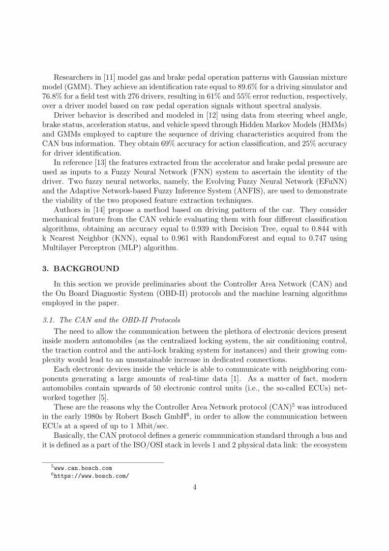
Researchers in [11] model gas and brake pedal operation patterns with Gaussian mixturemodel (GMM). They achieve an identification rate equal to 89.6% for a driving simulator and76.8% for a field test with 276 drivers, resulting in 61% and 55% error reduction, respectively,over a driver model based on raw pedal operation signals without spectral analysis.

Driver behavior is described and modeled in [12] using data from steering wheel angle,brake status, acceleration status, and vehicle speed through Hidden Markov Models (HMMs)and GMMs employed to capture the sequence of driving characteristics acquired from theCAN bus information. They obtain 69% accuracy for action classification, and 25% accuracyfor driver identification.

In reference [13] the features extracted from the accelerator and brake pedal pressure areused as inputs to a Fuzzy Neural Network (FNN) system to ascertain the identity of thedriver. Two fuzzy neural networks, namely, the Evolving Fuzzy Neural Network (EFuNN)and the Adaptive Network-based Fuzzy Inference System (ANFIS), are used to demonstratethe viability of the two proposed feature extraction techniques.

Authors in [14] propose a method based on driving pattern of the car. They considermechanical feature from the CAN vehicle evaluating them with four different classificationalgorithms, obtaining an accuracy equal to 0.939 with Decision Tree, equal to 0.844 withk Nearest Neighbor (KNN), equal to 0.961 with RandomForest and equal to 0.747 usingMultilayer Perceptron (MLP) algorithm.

3. BACKGROUND

In this section we provide preliminaries about the Controller Area Network (CAN) andthe On Board Diagnostic System (OBD-II) protocols and the machine learning algorithmsemployed in the paper.

3.1. The CAN and the OBD-II Protocols

The need to allow the communication between the plethora of electronic devices presentinside modern automobiles (as the centralized locking system, the air conditioning control,the traction control and the anti-lock braking system for instances) and their growing com-plexity would lead to an unsustainable increase in dedicated connections.

Each electronic devices inside the vehicle is able to communicate with neighboring com-ponents generating a large amounts of real-time data [1]. As a matter of fact, modernautomobiles contain upwards of 50 electronic control units (i.e., the so-called ECUs) net-worked together [5].

These are the reasons why the Controller Area Network protocol (CAN)5 was introducedin the early 1980s by Robert Bosch GmbH6, in order to allow the communication betweenECUs at a speed of up to 1 Mbit/sec.

Basically, the CAN protocol defines a generic communication standard through a bus andit is defined as a part of the ISO/OSI stack in levels 1 and 2 physical data link: the ecosystem

5www.can.bosch.com6https://www.bosch.com/

4

of the ECUs communicate with one another by sending CAN packets. These kinds of packetsare broadcast to all the components on the bus and each component decides whether it isintended for them, although segmented CAN networks do exist.

In practice, using the CAN protocol the ECU “A” is able to send data to the ECU “B”,but this is not enough to realize the communication: it is also necessary that the ECU “B”is able to recognize and use the data received by ECU “A”, for this reason it is necessarysomething that make able the two electronic control units to “speak the same language”.For this reason the OBD-II standard (On Board Diagnostics) [15] was introduced, in orderto define a common language that make the various ECUs able to communicate.

The OBD-II protocol is more specific than the CAN one and it is specifically createdas a standard for vehicles; it has become mandatory in America in vehicles manufacturedsince 1996. The European version of this standard is called European On Board Diagnostics(EOBD), it is substantially identical to the OBD-II one and it is mandatory since 20017.

The CAN and the OBD-II protocols cooperate in the following way: first of all, the OBD-II message is generated, then this the message becomes the content of the CAN messagethat is sent on the bus. The ECU that receives the CAN message makes the reverse process:it processes the message CAN, OBD-II drawing its original message and processes it.

Furthermore, OBD-II is not only a communication standard, it also defines the connectorthat must be present in the passenger compartment of the vehicle for connecting OBD-IIcompatible instruments8. This connector is essentially a port for the connection to the CANbus. In this way it is possible to extract the data from the CAN bus.

While the OBD-II standard has been mandatory for all cars and light trucks sold in theUnited States since 1996, the EOBD (i.e., the European On Board Diagnostics) standardhas been mandatory for all petrol vehicles sold in the European Union since 2001 and alldiesel vehicles since 2004. Both the OBD-II and the EOBD standards are available on carsand trucks.

Relating to the motorcycles, essentially, these vehicles are conform to the CAN protocolbut they do not exhibit an OBD-II connector. They present their own proprietary connectorand converters for the various manufacturers that do support the protocol standard and usethe OBD-II scan tool to retrieve information. The main problem from this point of viewis that, since there has not been a regulatory component mandating standardization formotorcycles, the various connection types have become proprietary as manufacturers try tomaintain their closed end to end systems.

3.2. Machine Learning

Machine learning is a type of artificial intelligence able to provide computers with theability to learn without being explicitly programmed [16].

Machine learning tasks are typically classified into two categories, depending on thenature of the learning available to a learning system:

7https://www.sae.org/events/pdf/obd-eu/2016_obd-eu_guide.pdf8http://www.obdii.com/connector.html

5

• Supervised learning : the computer is presented with example inputs and their desiredoutputs, given by a “teacher”, and the goal is to learn a general rule that maps inputsto outputs. It represents the classification: the process of building a model of classesfrom a set of records that contains class labels.

• Unsupervised learning : no labels are given to the learning algorithm, leaving it onits own to find structure in its input. Unsupervised learning can be a goal in itself(discovering hidden patterns in data) or a means towards an end (feature learning).

The algorithms considered are supervised decision tree-based i.e., they use a decision treeas a predictive model which maps observations about an item (represented in the branches) toconclusions about the target of the items value (represented in the leaves). These algorithms(i.e., J48, J48graft, J48consolidated, RandomTree, RepTree) are the most widespread to solvedata mining problems [16] for instance, from malware detection [17, 18, 19, 20] to pathologiesclassification [21].

In order to enforce the conclusion validity, we consider in this work five different machinelearning algorithms in order to demonstrate the effectiveness of our method in discriminatingbetween car owner and impostors.

4. THE METHOD

In this section we describe our method to identify driver behavior using data retrievedby CAN bus. As stated in the introduction, real data [14], processed from in-vehicle CANdata, are considered. In order to collect data, the On Board Diagnostics 2 (OBD-II) andCarbigsP as OBD-II scanner are used. The recent vehicle has many measurement sensorsand control sensors, so the vehicle is managed by ECU in it. ECU is the device that controlsparts of the vehicle such as Engine, Automatic Transmission, and Antilock Braking System(ABS). OBD refers to the self-diagnostic and reports capability by monitoring vehicle systemin terms of ECU measurement and vehicle failure. The data are recorded every 1 secondduring driving.

We considered a real-environment and not a simulated one in order to examine all possiblereal-world variables, for instance: slowdowns traffic lights and all the possible variables thatare not considerable in a simulated environment.

The total number of the collected features is 51. Table 1 describes the features involvedin the study. The data are related to a recent model of KIA Motors Corporation in SouthKorea.

Table 1: Features involved in the study.

# Feature Description1 Fuel consumption The instant value related to fuel consumption

table continues on next page

6

Table 1 –table continues from the previous page# Feature Description2 Accelerator Pedal value This sensor registers the movement of the accelerator

pedal: Accelerator pedal opening angle percentage asdetermined by the accelerator position sensor.

3 Throttle position signal The relative throttle position sensor is used to mon-itor the throttle position of a vehicle

4 Short Term Fuel Trim Bank1 Fuel trims are the percentage of change in fuel overtime in short term

5 Intake air pressure This data is used to calculate air density and deter-mine the engine’s air mass flow rate

6 Filtered Accelerator Pedal valueECU’s filtered accelerator pedal opening angle per-centage as determined by the accelerator positionsensor.

7 Absolute throttle position Actual position of the throttle8 Engine soacking time Duration of time a vehicle’s engine is at rest prior to

being started.9 Inhibition of engine fuel cut off The fuel cut-off control system is responsive to a

brake switch signal and an engine speed signal havinga value above a fuel recovery threshold to decreasethe value of a fuel cut-off threshold to again per-form the fuel cut-off even in the normal fuel recoveryrange. This value represents the inhibition of enginefuel cut off

10 Engine in fuel cut off This value represents the inhibition of engine fuel cutoff, i.e., fuel cut-off threshold.

11 Fuel Pressure Effective pressure is the actual applied pressure forthe injector, and is the pressure differential acrossthe injector.

12 Long Term Fuel Trim Bank1 Fuel trims are the percentage of change in fuel overtime in long term.

13 Engine speed It is also called engine’s RPM, i.e., Revolutions PerMinute. In other words it is the number of revolu-tions the crankshaft makes per minute.

14 Engine torque after correction The value after correcting the torque to which anengine is adjusted before a gear disengagement.

15 Torque of friction Friction torque is the torque caused by the frictionalforce that occurs when two objects in contact move.

table continues on next page

7

Table 1 –table continues from the previous page# Feature Description16 Flywheel torque interventions The flywheel stores energy when torque is applied

by the energy source, and it releases stored energywhen the energy source is not applying torque to it.The value represent the flywheel torque after torqueinterventions.

17 Current spark timing The time to set the angle relative to piston positionand crankshaft angular velocity that a spark will oc-cur in the combustion chamber near the end of thecompression stroke.

18 Engine coolant temperature The temperature of the engine coolant of the internalcombustion engine

19 Engine Idle Target Speed The desired idle RPM in relation to coolant temp.20 Engine torque Engine torque is also related to the gearing. The

lower the gear, greater is the pulling ability of anengine and hence greater the torque that this valuerepresents.

21 Calculated LOAD value This value indicates a percentage of peak availabletorque.

22 Min indicated engine torque Minimum Engine torque value23 Max indicated engine torque Maximum Engine torque value24 Flywheel torque The value represent the flywheel torque25 Torque scaling factor This value is described as how flexible or how much

force can be expressed in a given gear when the driverscales the gear.

26 Standard Torque Ratio This value is described as how flexible or how muchforce can be expressed in a given gear.

27 Requested spark retard angle The transmission control unit (TCU) controls mod-ern electronic automatic transmissions. This valuecomputes the requested spark retard angle fromTCU.

28 Requests engine torque limit This parameter monitors the request to enginetorque limits (ETL) by TCU

29 Requested engine RPM increaseThis parameter monitors the TCU requests relatedto the RPM engine increasing

30 Target engine speed usedin lock-up module

It monitors the lock-up valve, used to shut off thesignal pressure line of pneumatic actuators.

31 Glow plug control request It monitors the request to check the glow plug32 Activation of Air compressor The value of the air compressor’s working.

table continues on next page

8

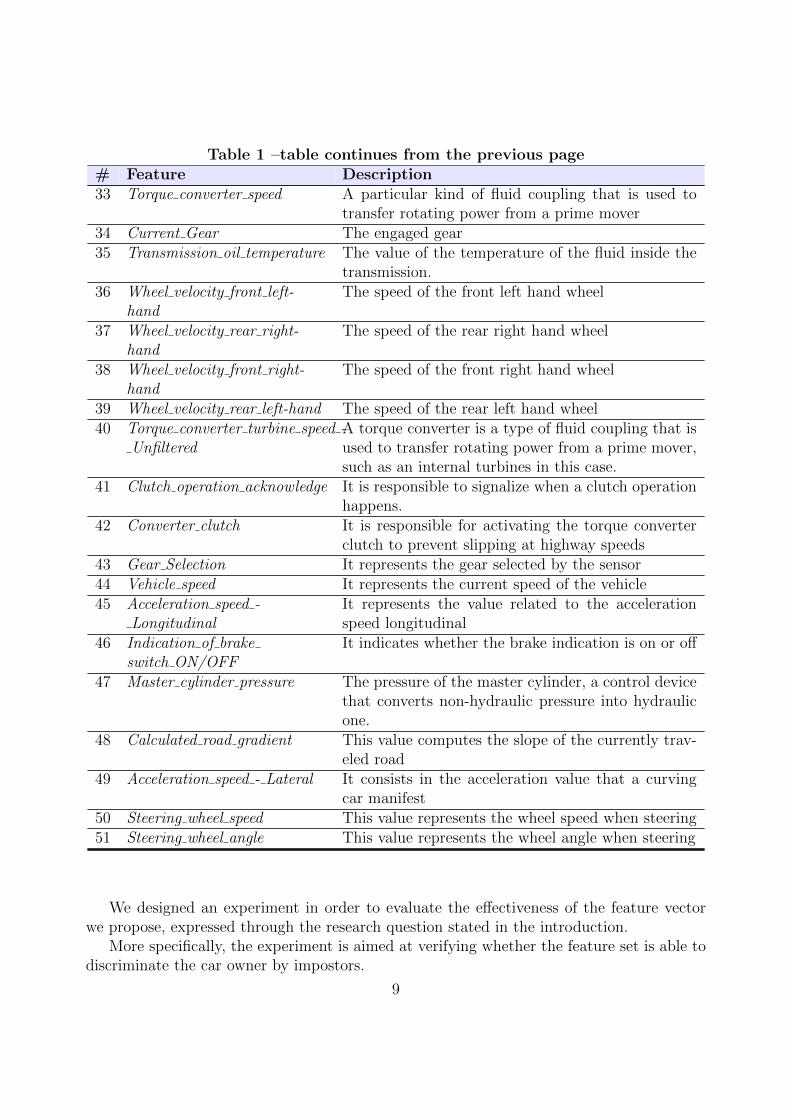
Table 1 –table continues from the previous page# Feature Description33 Torque converter speed A particular kind of fluid coupling that is used to

transfer rotating power from a prime mover34 Current Gear The engaged gear35 Transmission oil temperature The value of the temperature of the fluid inside the

transmission.36 Wheel velocity front left-

handThe speed of the front left hand wheel

37 Wheel velocity rear right-hand

The speed of the rear right hand wheel

38 Wheel velocity front right-hand

The speed of the front right hand wheel

39 Wheel velocity rear left-hand The speed of the rear left hand wheel40 Torque converter turbine speed -

UnfilteredA torque converter is a type of fluid coupling that isused to transfer rotating power from a prime mover,such as an internal turbines in this case.

41 Clutch operation acknowledge It is responsible to signalize when a clutch operationhappens.

42 Converter clutch It is responsible for activating the torque converterclutch to prevent slipping at highway speeds

43 Gear Selection It represents the gear selected by the sensor44 Vehicle speed It represents the current speed of the vehicle45 Acceleration speed -

LongitudinalIt represents the value related to the accelerationspeed longitudinal

46 Indication of brakeswitch ON/OFF

It indicates whether the brake indication is on or off

47 Master cylinder pressure The pressure of the master cylinder, a control devicethat converts non-hydraulic pressure into hydraulicone.

48 Calculated road gradient This value computes the slope of the currently trav-eled road

49 Acceleration speed - Lateral It consists in the acceleration value that a curvingcar manifest

50 Steering wheel speed This value represents the wheel speed when steering51 Steering wheel angle This value represents the wheel angle when steering

We designed an experiment in order to evaluate the effectiveness of the feature vectorwe propose, expressed through the research question stated in the introduction.

More specifically, the experiment is aimed at verifying whether the feature set is able todiscriminate the car owner by impostors.

9

The classification is carried out by using well-known classifiers built with the feature setas explained in Section 3.

The evaluation consists of three stages: (i) comparison of descriptive statistics of thepopulations of the drivers; (ii) hypotheses testing, in order to verify whether the featurespresent different distributions for the populations of the drivers; and (iii) a classificationanalysis aimed at assessing whether the features are able to correctly classify between carowner and impostors.

Relating to the descriptive statistics, we report the box plot of the distribution of thedrivers involved in the study in order to demonstrate that the distributions are different.

With regards to the hypotheses testing, the null hypothesis to be tested is:H0: “the drivers have similar values of the considered features”.The null hypothesis was tested with Wald-Wolfowitz (with the p-level fixed to 0.05),

Mann-Whitney (with the p-level fixed to 0.05) and with Kolmogorov-Smirnov Test (withthe p-level fixed to 0.05). We chose to run three different tests in order to enforce theconclusion validity.

The purpose of these tests is to determine the level of significance, i.e., the risk (theprobability) that erroneous conclusions be drawn: in our case, we set the significance levelequal to .05, which means that we accept to make mistakes 5 times out of 100.

The classification analysis was aimed at assessing whether the feature set is able tocorrectly classify car owner and impostors.

We adopt the supervised learning approach, considering that the driver features evaluatedin this work contain the driver labels.

The supervised learning approach is composed of two different steps:

1. Learning Step: starting from the labeled dataset (i.e., where each feature is relatedto a class. In our case, the class is represented by the driver), we filter the data in orderto obtain a feature vector. The feature vectors, belonging to all the drivers involved inthe experiment with the associated labels, represent the input for the machine learningalgorithm that is able to build a model from the analyzed data. The output of thisstep is the model obtained by the labeled dataset.

2. Prediction Step: the output of this step is the classification of a feature vectorbelonging to the car owner or to an impostor. Using the model built in the previousphase, we input this model using a feature vector without the label: the classifier willoutput with their label prediction (i.e., car owner or impostor).

In addition, we perform a principal component analysis (PCA) [22, 23] in order to iden-tify, from the 51 features involved, the best features discriminating the driver behavior. Weemploy two different algorithms: BestFirst [22] and GreedyStepwise [24]. In case the PCAanalysis is able to return the best features, we classify the new feature set with the classi-fication algorithms in order to compare the previous results obtained using the full featureset.

Figure 1 represents the flow diagram of the proposed approach.The most important step is represented by the selection block in Figure 1: in this block

the feature set is acquired from the OBD and it is evaluated against the learned model in

10

Figure 1: The flow diagram of the proposed approach.

order to decide whether it belongs to the car owner.The classification analysis was accomplished with Weka9, a suite of machine learning

software, largely employed in data mining for scientific research.In the following, we present two possible scenarios related to the adoption of the proposed

method in two different fields. The first one (i.e., the anti-theft instrument) is depicted inFigure 2, while the second one (the car insurance company tool) is depicted in Figure 3.

Figure 2: An example of utilization of the proposed solution in order to identity car theft. In the upper box(i.e., Scenario 1) an example of the usage of the proposed method when the car owner is driving own car,while in the lower box (i.e., Scenario 2) an example of the usage of the proposed method when a car thiefis driving the owner car: in this case the proposed method sends an alert to the car owner mobile device.

The scenarios shown in Figure 2 are related to two cases: the first one (i.e., Scenario1) related to the car owner when is driving the own car, in this case the case the proposedmethod will recognize the driver as the car owner and the proposed method will not sendan alert; differently in the second case (i.e., Scenario 2) the car owner will receive an alertthrough their mobile device because the proposed method does not recognize the drivingstyle as belonging to the car owner.

9http://www.cs.waikato.ac.nz/ml/weka/

11

The second area of applicability of the proposed solution is related to car insurance, thecorresponding scenario is represented in Figure 3.

Figure 3: An example of usage of the proposed method useful for car insurance companies proposing driveraccident policy. In this scenario the vehicles under analysis send periodically the data to the company serversin order to store and analyze the data with the aim to identify whether the driver is the car owner.

While in the anti-theft scenario the controls about the driving style are performed intothe mobile device car owner (that also receives the feature set gathered from the own car), inthis scenario the feature sets of different vehicles are sent to the company insurance serversin order to be analyzed. As a matter of fact, several car insurance companies are proposingpolicy driver-oriented: driver accident policy is an accessory guarantee that allows peopleto receive financial compensation in case of bodily injury suffered by the driver, only in thecase of a faulted fault. In this case the main problem, from the car insurance company pointof view, is to establish who is driving the car at the time of the accident. Furthermore,considering that the car insurance is able also to determine whether the car is guided bythe insured or from another person, this can be considered as deterrent for the car owner togive own car to other people.

5. THE EVALUATION

In this section we describe the real-world dataset used in this paper and the results ofthe experiment.

For the sake of clarity, the results of the evaluation will be discussed reflecting thedata analysis’ division in three phases discussed in previous section: descriptive statistics,hypotheses testing and classification.

5.1. The Dataset

Ten different drivers participated to the experiment by driving, with the same car, 4different round-trip paths in Seoul (i.e., between Korea University and SANGAM WorldCup Stadium) for about 23 hours of total driving time. Figure 4 shows the path consideredby the different participant drivers.

12

Figure 4: Path from Korea University to Seoul World Cup Stadium.

The driving paths are of three types: city way, motor way and parking space with a totallength of about 46 km. The experiment is performed since July 28, 2015. The experimentswere performed in the similar time zone from 8 p.m to 11 p.m on weekdays. The ten drivers,labeled from “A” to “J”, completed two round trips for reliable classification, while dataare collected from totally different road conditions. The city way has signal lamps andcrosswalks, but the motor way has none. The parking space is required to drive slowly andcautiously.

The data that we have used has total 94,401 items recorded every second with the sizeof 16.7Mb in total and it is freely available for research purpose10.

5.2. Descriptive statistics

Figures 5, 6, 7 and 8 show the box plots related to the Fuel consuption (i.e., the featurenumber #1 in Table 1), the Intake air pressure (i.e., the feature number #5 in Table 1), theLong Term Fuel Trim Bank1 (i.e., the feature number #12 in Table 1) and the Transmis-sion oil temperature (i.e., the feature number #35 in table 1). Considering the big numberof features, we do not show the box plot related to the full set composed of the 51 features,but a similar consideration can be done for all the features involved in the study.

The box plots in Figure 5 present the distributions for the 10 drivers related to theFuel consuption feature. This feature ranges between 0 and 10000 and it is measured incubic millimeter (mcc).

The 10 drivers present a similar distribution; considering that the Fuel consuption featurecan be correlated to the Accelerator pedal value (more pressure on the accelerator pedalincreases the speed of the vehicle and then more fuel is required) the driver A presents aslightly larger box plot if compared with other drivers.

The box plots in Figure 6 show the driver distribution related to Intake air pressurefeature (i.e., the pressure of air inhaled to engine). It ranges between 0 and 255, and it ismeasured in Kilopascal (kPA).

From the analysis of the Intake air pressure, it seems that engines of A, E and J driversinhale similar pressure of air (ranging between 45 and 60 kPA) while, the remaining engine

10https://sites.google.com/a/hksecurity.net/ocslab/Datasets/driving-dataset

13

Figure 5: Box plots related to the the Fuel consuption feature (i.e., the number #1 in table 1) for the tendifferent drivers considered in the experiment.

Figure 6: Box plots related to the Intake air pressure feature (i.e., the number #5 in table 1) for the tendifferent drivers considered in the experiment.

drivers (B, C, D, F, G, H and I) need to an air pressure ranging between 0 and 50 kPA.Considering that the air intake pressure is influenced by the degree of opening throttle platewhich draws the fuel to the combustion chamber in engine [25], a bigger air pressure will bereflected in fuel increased consumption.

The Long Term Fuel Trim#Bank1 feature box plots are shown in Figure 7. This featurerepresents, in percentage, the correction value being used by the fuel control system in loopmodes of operation and it is expressed in percentage. We explain how the correction valueworks in detail: basically, fuel trims are defined as the percentage of change in fuel overtime. For engines that work correctly, the ratio between air and fuel must be included in asmall interval. There are several conditions that make this interval too wide, for instance,cold start-up, cruising down the highway and idling in heavy traffic.

The engine computer tries to perform the best in order to maintain this proper ratiobetween air and fuel by fine-tuning the amount of fuel going into the engine: it adds ortakes away fuel, the oxygen sensors monitor how much oxygen is in the exhaust and respondby telling it to the engine computer.

This change in fuel being added or taken away is called Fuel Trim. The oxygen sensorsare what drive the fuel trim readings. Changes in O2 sensor voltages cause a direct change

14

in fuel. The short term fuel trim (STFT) refers to immediate changes in fuel occurringseveral times per second. The long term fuel trims (LTFT) are driven by the short termfuel trims. LTFT refers to changes in STFT but averaged over a longer period of time. Anegative fuel trim percentage indicates a taking away of fuel, while a positive percentageindicates an adding of fuel. STFT are immediate ups and downs in fuel, while LTFT arewhat is occurring over a longer period.

Figure 7: Box plots related to the Long Term Fuel Trim#Bank1 feature (i.e., the number #12 in table 1)for the ten different drivers considered in the experiment.

The Long Term Fuel Trim Bank1 feature distributions show different trends betweenthe 10 drivers. As a matter of fact, the A driver exhibits the lowest distribution, while the Eone the most greater one. All the remaining drivers (i.e., B, C, F, G, H, I and J) present boxplots ranging between 2% and 6%. Driver D exhibits the most tiny box plot. Consideringthat this value is increased when conditions, like cold start-up, cruising down the highwayand idling in heavy traffic, happen, we think that this feature (and the box plot confirmsour hypothesis) can be very useful in order to discriminate car owner from impostors.

The box plots related to the Transmission oil temperature are represented in Figure 8:it represents the oil temperature inside the transmission and it is ranging between -40 and215 Celsius degree.

Figure 8: Box plots related to the Transmission oil temperature feature (i.e., the number #35 in table 1)for the ten different drivers considered in the experiment.

The A driver presents the highest value for this feature: 100 Celsius degree. For the

15

remaining drivers, the value ranges between 85 and 95 Celsius degree: this is consideredas a normal value. The only exception is represented by the E driver engine with lowesttemperature values. Considering that an engine in good conditions is able to reach the sameoil temperature degree, this feature seems to be not indicative for drivers discrimination(and the box plots seem to confirm our hypothesis).

5.3. Hypothesis testing

The hypothesis testing aims at evaluating if the features present different distributionsfor the populations of the 10 drivers involved in the experiment with statistical evidence.

We assume valid the results when the null hypothesis is rejected by the three testsperformed.

Table 2 shows the null hypothesis H0 test.

Table 2: Results of the null hypothesis H0 test.

# Feature Wald-Wolfowitz Mann-Whitney Kolmogorov-Smirnov Test Result[1− 2] 0,000 0,000 p < .001 passed

3 0,000 0,000047 p < .001 passed4 0,000 0,227366 p < .001 not passed5 0,000 0,000 p < .001 passed6 0,000 1,000 p > .10 not passed7 0,000 0,000121 p < .001 passed8 0,000 0,000 p < .001 passed9 0,000 1,000 p > .10 not passed10 0.000 0,488959 p > .10 not passed11 0,000 1,000 p > .10 not passed

[12− 21] 0,000 0,000 p < .001 passed22 0,000 0,495956 p < .001 not passed23 0,000 0,004297 p < .001 passed24 0,000 0,000 p < .001 passed

[25− 27] 0,000 1,000 p > .10 not passed28 0,000 0,09627 p > .10 not passed29 0,000 0,000 p > .10 not passed

[30− 32] 0,000 1,000 p > .10 not passed33 0,000 0,000 p < .001 passed34 0,000 0,951169 p < .001 not passed35 0,000 0,000 p < .001 passed36 0,000 0,000002 p < .001 passed37 0,000 0,000005 p < .001 passed38 0,000 0,000006 p < .001 passed39 0,000 0,000002 p < .001 passed

[40− 42] 0,000 0,000 p < .001 passed43 0,000 0,338733 p > .10 not passed44 0,000 0,000005 p < .001 passed

[45− 49] 0,000 0,000 p < .001 passed50 0,000 0,33013 p < .01 not passed51 0,000 0,727628 p < .001 not passed

All the features are able to successfully pass the Wald-Wolfowitz test, while the Mann-Whitney test is not passed by features #4,#6,#10,#22,#25,#26, #27, #34, #43, #51 andthe Kolmogorov-Smirnov test is not passed by features #6, #9, #10, #11, #25, #26, #27,#28, #29, #30, #31, #43. We highlight that features #6, #10, #25, #26 and #27 notpassed both the Mann-Whitney test and the Kolmogorov-Smirnov one. This is symptomatic

16

that in the dataset not all the features contribute to discriminate different drivers, especiallywhen the features have not passed two tests on three.

To summarize, considering that we assume valid the results when the null hypothesis isrejected by the three tests performed, the features that have not passed the null hypothesisH0 test are: #4, #6, #9, #10, #11, #22, #25, #26, #27, #28, #29, #30, #31, #34, #43,#51 i.e., 17 features on the 51 considered in the study: the classification analysis with thefeature selection will confirm whether these resulting features are not able to discriminatebetween the different drivers involved in the study.

5.4. Classification analysis

We classified the features extracted using five classification algorithms: J48, J48graft,J48consolidated, RandomTree and RepTree.

Five metrics were used to evaluate the classification results: False Positive (FP) rate,Precision, Recall, F-Measure and ROC Area.

The FP rate is calculated as the ratio between the number of negative driver traceswrongly categorized as belonging to the owner (i.e.,the false positives) and the total numberof actual impostor traces (i.e., the true negatives): FP rate = fp

fp+tn, where fp indicates the

number of false positives and tn the number of true negatives.The Precision has been computed as the proportion of the examples that truly belong

to class X among all those which were assigned to the class. It is the ratio of the number ofrelevant records retrieved to the total number of irrelevant and relevant records retrieved:Precision = tp

tp+fp, where tp indicates the number of true positives and fp indicates the

number of false positives.The Recall has been computed as the proportion of examples that were assigned to class

X, among all the examples that truly belong to the class, i.e., how much part of the classwas captured. It is the ratio of the number of relevant records retrieved to the total numberof relevant records: Recall = tp

tp+fn, where tp indicates the number of true positives and fn

indicates the number of false negatives.The F-Measure is a measure of a test’s accuracy. This score can be interpreted as a

weighted average of the precision and recall: F-Measure = 2 ∗ Precision∗RecallPrecision+Recall

.The Roc Area is defined as the probability that a positive instance randomly chosen is

classified above a negative randomly chosen.The classification analysis consisted of building classifiers in order to evaluate feature

accuracy to distinguish the car owner by an impostor.We consider two different approaches in order to build the model starting from the

feature.In the first one, the multi driver classification, for training the first classifier, we defined

T as a set of labeled behavioral traces (BT, l), where each BT is associated to a label l ∈{A, B, C, D, E, F, G, H, I, J}.

For training the second classifier, i.e., the binary one, we defined T as a set of labeledbehavioral traces (BT, l), where each BT is associated to a label l ∈ {impostor, owner}.For each BT we built a feature vector F ∈ Ry , where y is the number of the features usedin training phase (y = 51).

17

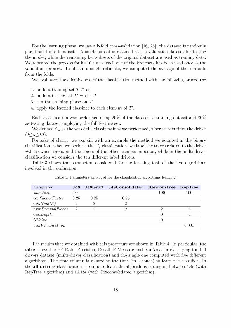
For the learning phase, we use a k-fold cross-validation [16, 26]: the dataset is randomlypartitioned into k subsets. A single subset is retained as the validation dataset for testingthe model, while the remaining k-1 subsets of the original dataset are used as training data.We repeated the process for k=10 times; each one of the k subsets has been used once as thevalidation dataset. To obtain a single estimate, we computed the average of the k resultsfrom the folds.

We evaluated the effectiveness of the classification method with the following procedure:

1. build a training set T ⊂ D;

2. build a testing set T ′ = D ÷ T ;

3. run the training phase on T ;

4. apply the learned classifier to each element of T ′.

Each classification was performed using 20% of the dataset as training dataset and 80%as testing dataset employing the full feature set.

We defined Cu as the set of the classifications we performed, where u identifies the driver(1≤u≤10 ).

For sake of clarity, we explain with an example the method we adopted in the binaryclassification: when we perform the C2 classification, we label the traces related to the driver#2 as owner traces, and the traces of the other users as impostor, while in the multi driverclassification we consider the ten different label drivers.

Table 3 shows the parameters considered for the learning task of the five algorithmsinvolved in the evaluation.

Table 3: Parameters employed for the classification algorithms learning.

Parameter J48 J48Graft J48Consolidated RandomTree RepTree

batchSize 100 100 100

confidenceFactor 0.25 0.25 0.25

minNumObj 2 2 2

numDecimalPlaces 2 2 2 2 2

maxDepth 0 -1

KValue 0

minVarianteProp 0.001

The results that we obtained with this procedure are shown in Table 4. In particular, thetable shows the FP Rate, Precision, Recall, F-Measure and RocArea for classifying the fulldrivers dataset (multi-driver classification) and the single one computed with five differentalgorithms. The time column is related to the time (in seconds) to learn the classifier. Inthe all drivers classification the time to learn the algorithms is ranging between 4.4s (withRepTree algorithm) and 16.18s (with J48consolidated algorithm).

18

Table 4: Classification results.

Family Algorithm FP Rate Precision Recall F-Measure Roc Area TimeJ48 0.001 0.992 0.992 0.992 0.998 15.95sJ48graft 0.001 0.992 0.992 0.992 0.998 16.04s

All drivers J48consolidated 0.001 0.991 0.991 0.991 0.998 16.18sRandomTree 0.014 0.880 0.880 0.880 0.933 1.07sRepTree 0.002 0.987 0.987 0.987 0.998 4.40sJ48 0.000 0.998 0.997 0.998 0.999 14.04sJ48graft 0.000 0.998 0.996 0.997 0.999 16.02s

Driver A J48consolidated 0.000 0.997 0.995 0.996 0.999 15.98sRandomTree 0.004 0.956 0.944 0.950 0.970 0.99sRepTree 0.000 0.997 0.996 0.996 1.000 4.10sJ48 0.001 0.991 0.994 0.992 0.998 7.96sJ48graft 0.002 0.990 0.994 0.992 0.998 7.99s

Driver B J48consolidated 0.002 0.990 0.990 0.990 0.998 6.98sRandomTree 0.015 0.902 0.898 0.900 0.941 1.48sRepTree 0.002 0.987 0.986 0.986 0.998 3.67sJ48 0.001 0.991 0.992 0.991 0.997 8.95sJ48graft 0.001 0.990 0.991 0.991 0.997 8.99s

Driver C J48consolidated 0.001 0.985 0.992 0.989 0.997 9.06sRandomTree 0.015 0.823 0.826 0.824 0.905 1.19sRepTree 0.002 0.977 0.979 0.978 0.998 4.15sJ48 0.002 0.991 0.988 0.989 0.996 12.04sJ48graft 0.001 0.992 0.987 0.990 0.996 12.01s

Driver D J48consolidated 0.002 0.988 0.981 0.984 0.997 11.58sRandomTree 0.022 0.862 0.863 0.863 0.92 1.49sRepTree 0.003 0.979 0.979 0.979 0.997 5.59sJ48 0.000 0.997 0.998 0.997 1.000 9.30sJ48graft 0.000 0.996 0.998 0.997 0.999 9.12s

Driver E J48consolidated 0.001 0.995 0.997 0.996 0.999 9.10sRandomTree 0.005 0.949 0.954 0.952 0.974 0.50sRepTree 0.000 0.996 0.997 0.996 0.999 2.71sJ48 0.001 0.994 0.996 0.995 0.999 4.47sJ48graft 0.001 0.993 0.996 0.994 0.999 4.54s

Driver F J48consolidated 0.001 0.992 0.994 0.993 0.999 4.22sRandomTree 0.012 0.913 0.917 0.915 0.953 1.09sRepTree 0.001 0.992 0.992 0.992 0.999 3.14sJ48 0.001 0.992 0.991 0.992 0.997 13.38sJ48graft 0.001 0.992 0.991 0.992 0.997 13.47s

Driver G J48consolidated 0.001 0.991 0.990 0.990 0.997 13.29sRandomTree 0.010 0.881 0.885 0.883 0.937 1.55sRepTree 0.001 0.984 0.984 0.984 0.998 5.12sJ48 0.001 0.993 0.993 0.993 0.998 12.66sJ48graft 0.001 0.993 0.993 0.993 0.998 12.71s

Driver H J48consolidated 0.001 0.990 0.990 0.990 0.998 12.67sRandomTree 0.018 0.844 0.852 0.848 0.917 1.80sRepTree 0.002 0.986 0.987 0.986 0.998 5.40sJ48 0.001 0.988 0.988 0.988 0.997 8.64sJ48graft 0.001 0.990 0.988 0.989 0.997 8.58s

Driver I J48consolidated 0.001 0.991 0.994 0.993 0.998 8.41sRandomTree 0.018 0.808 0.816 0.812 0.899 1.11sRepTree 0.001 0.988 0.984 0.986 0.998 4.36sJ48 0.001 0.990 0.988 0.989 0.997 9.03sJ48graft 0.001 0.990 0.990 0.990 0.997 9.07s

Driver J J48consolidated 0.001 0.990 0.990 0.990 0.998 9.17sRandomTree 0.015 0.856 0.838 0.846 0.911 1.07sRepTree 0.002 0.984 0.986 0.985 0.998 3.78s

19

In the multi driver classification (All drivers family) we obtain following best resultsfrom the point of the views of the metrics we considered:

• FP rate equal to 0.001 with the J48, J48graft and J48consolidated algorithms;

• Precision, Recall and F-Measure equal to 0.992 using the J48 and the J48graft classi-fication algorithms;

• Roc Area equal to 0.998 using J48, J48graft, J48consolidated and RepTree classifica-tion algorithms.

The reader can find in Table 4 the single driver results, while Table 5 shows the fea-ture selection results. The two feature selection algorithms employed, the BestFirst and theGreedyStepwise, confirm that 6 features on the 51 considered in the full features datasetare the most discriminatory in driver identification i.e., the #5 (Intake air pressure), the #8(Engine soacking time), the #12 (Long Term Fuel Trim Bank1 ), the #15 (Torque of friction),the #35 (Transmission oil temperature) and the #50 (Steering wheel speed) features.

As expected, all the six features resulting from the feature selection step successfullypassed the null hypothesis H0 test, as shown in Table 2.

Table 5: Feature Selection Results.

# Feature

5 Intake air pressure

8 Engine soacking time

12 Long Term Fuel Trim Bank1

15 Torque of friction

35 Transmission oil temperature

50 Steering wheel speed

Table 6 shows the classification analysis considering the features retrieved from the fea-ture selection step.

20

Table 6: Best Features Classification results.

Family Algorithm FP Rate Precision Recall F-Measure Roc Area TimeJ48 0.001 0.989 0.989 0.989 0.998 1.69sJ48graft 0.001 0.990 0.99 0.990 0.997 1.58s

All drivers J48consolidated 0.002 0.986 0.986 0.986 0.998 1.71sRandomTree 0.002 0.984 0.984 0.984 0.991 0.41sRepTree 0.002 0.984 0.984 0.984 0.998 0.54sJ48 0.000 0.998 0.997 0.998 0.999 1.33sJ48graft 0.000 0.997 0.997 0.997 0.999 1.29s

Driver A J48consolidated 0.000 0.997 0.997 0.997 0.999 1.36sRandomTree 0.000 0.997 0.996 0.997 0.998 0.25sRepTree 0.000 0.997 0.996 0.997 1.000 0.49sJ48 0.001 0.991 0.991 0.991 0.998 3.26sJ48graft 0.002 0.990 0.992 0.991 0.998 3.18s

Driver B J48consolidated 0.002 0.988 0.985 0.987 0.998 3.23sRandomTree 0.002 0.986 0.987 0.986 0.992 0.35sRepTree 0.002 0.986 0.987 0.986 0.998 0.47sJ48 0.002 0.980 0.979 0.980 0.997 2.36sJ48graft 0.002 0.982 0.979 0.98 0.996 2.25s

Driver C J48consolidated 0.002 0.972 0.983 0.977 0.997 2.45sRandomTree 0.002 0.974 0.971 0.972 0.984 0.39sRepTree 0.002 0.973 0.972 0.972 0.997 0.42sJ48 0.002 0.987 0.984 0.985 0.997 4.71sJ48graft 0.002 0.987 0.986 0.986 0.996 4.79s

Driver D J48consolidated 0.002 0.985 0.973 0.979 0.997 4.69sRandomTree 0.003 0.980 0.980 0.980 0.988 0.46sRepTree 0.003 0.980 0.974 0.977 0.997 0.79sJ48 0.000 0.997 0.997 0.997 0.999 1.64sJ48graft 0.000 0.998 0.997 0.998 0.999 1.58s

Driver E J48consolidated 0.000 0.996 0.996 0.996 0.999 1.62sRandomTree 0.001 0.995 0.996 0.995 0.998 0.27sRepTree 0.000 0.996 0.995 0.995 0.999 0.49sJ48 0.001 0.990 0.991 0.990 0.998 1.23sJ48graft 0.001 0.990 0.991 0.991 0.998 1.27s

Driver F J48consolidated 0.002 0.984 0.987 0.986 0.998 1.25sRandomTree 0.002 0.986 0.988 0.987 0.993 0.32sRepTree 0.002 0.984 0.986 0.985 0.999 0.31sJ48 0.000 0.995 0.995 0.995 0.999 2.28sJ48graft 0.001 0.994 0.995 0.994 0.999 2.34s

Driver G J48consolidated 0.001 0.991 0.994 0.992 0.998 2.31sRandomTree 0.001 0.989 0.989 0.989 0.994 0.38sRepTree 0.001 0.989 0.990 0.989 0.999 0.51sJ48 0.002 0.986 0.988 0.987 0.998 4.11sJ48graft 0.001 0.988 0.987 0.988 0.997 4.07s

Driver H J48consolidated 0.002 0.982 0.986 0.984 0.998 4.05sRandomTree 0.002 0.980 0.981 0.980 0.989 0.53sRepTree 0.003 0.978 0.982 0.980 0.998 0.85sJ48 0.002 0.982 0.985 0.983 0.996 2.79sJ48graft 0.001 0.984 0.985 0.985 0.997 2.67s

Driver I J48consolidated 0.002 0.976 0.984 0.980 0.996 2.87sRandomTree 0.002 0.979 0.974 0.977 0.986 0.28sRepTree 0.002 0.976 0.982 0.979 0.998 0.43sJ48 0.001 0.988 0.986 0.987 0.997 2.51sJ48graft 0.001 0.987 0.987 0.987 0.997 2.43s

Driver J J48consolidated 0.001 0.986 0.983 0.984 0.997 2.56sRandomTree 0.003 0.976 0.978 0.977 0.988 0.33sRepTree 0.002 0.981 0.976 0.979 0.997 0.51s

21

Table 6 shows the FP Rate, Precision, Recall, F-Measure and RocArea for classifyingthe full drivers dataset and the single one computed with the five different algorithms. Thetime column is related to the time (in seconds) to learn the classifier. In the all driversclassification the time to learn the algorithms is ranging between 0.41s (with the RandomTreealgorithm) and 1.71s (with the J48consolidated algorithm). Without PCA analysis theJ48consolidated algorithm employs 16.18s to learn the classifier. The obtained results interms of the analyzed metrics are closed to the previous ones, confirming that the excludedfeatures were not useful in the classification task. Indeed, in the second classification weconsidered only 6 features on the 51 considered in the previous one: the use of 6 featuresinstead of 51 is reflected in a higher applicability of the proposed method in the real world.As a matter of fact, the use of a lower number of features is reflected in a smaller storagespace and in a shorter computing time in order to identify the driver impostor.

In the multi driver classification, using the best features (All drivers family), we obtainthe following best results from the point of the views of the metrics we considered:

• FP rate equal to 0.001 with the J48 and J48graft algorithms;

• Precision, Recall and F-Measure equal to 0.989 using the J48 and the J48graft classi-fication algorithms;

• Roc Area equal to 0.998 using J48, J48consolidated, and RepTree classification algo-rithms.

In order to have a full vision about the single driver identification, we represent usinghistogram the obtained performance by the classification algorithms only for the FP rateconsidering the classification algorithm able to reach the best performance in the best featureclassification i.e., the J48 algorithm.

Figure 9 shows the FP Rate obtained classifying using the six best features with the J48algorithm. The FP Rate refers to the 10 drivers involved in the experiment. The FP Rateranges between 0 and 0.002. This results demonstrate that the number of false positives ofour methods is very low i.e., it is equal to 0.002 in the worst case (related to C, D, H andI drivers). Drivers A, E and G exhibit the best case with a FP rate equal to 0, while B, Fand J drivers obtain an FP rate equal to 0.001.

6. CONCLUSIONS AND FUTURE WORK

Modern vehicles, differently by older ones, integrate a lot of sophisticated electronicdevices. This increasing technologies permitted to find new way to steal cars, for instanceby exploiting the vulnerabilities of the operating system embedded in today’s car. Thisscenario calls for new methodologies in order to stem the phenomenon resulting from theintroduction of computers in the car, with the consequent vulnerability of software used. Inthis paper, we propose a method able to discriminate an impostor by the car owner using aset of characteristics available by the sensor embedded into the car. Using machine learningtechniques, we design several classifiers able to evaluate the effectiveness of our method: as

22

Figure 9: FP Rate values for the 10 drivers involved in the experiment obtained classifying the best featuresusing the J48 algorithm.

a matter of fact we obtain, in average, a precision and a recall equal to 0.99 in car ownerdiscrimination. As a future work, we plan to take into account in our model the type of theroad in order to design a system able to advise the user about the driving style to adopt.

A weakness of the proposed method is represented by the time-windows required tocollect the features to learn the classification algorithms; this is a common problem toall machine learning based solutions. As an additional future work, we will evaluate theminimum time-window able to guarantee performances over a certain threshold.

Moreover, we will extend the evaluation considering features extracted by trucks andmotorcycles with the aim to identify thefts not only cars-related.

Acknowledgments

This work has been partially supported by H2020 EU-funded projects NeCS and C3ISPand EIT-Digital Project HII and PRIN “Governing Adaptive and Unplanned Systems ofSystems” and the EU project CyberSure 734815.

Author Contributions

Fabio Martinelli, Francesco Mercaldo, Albina Orlando, Vittoria Nardone, Antonella San-tone and Arun Kumar Sangaiah are all responsible for the concept of the paper, the resultspresented and the writing. All the authors have read and approved the final publishedmanuscript.

References

[1] F. Martinelli, F. Mercaldo, V. Nardone, and A. Santone, “Car hacking identification through fuzzylogic algorithms,” in Fuzzy Systems (FUZZ-IEEE), 2017 IEEE International Conference on. IEEE,2017, pp. 1–7.

23

[2] K. M. A. Alheeti, A. Gruebler, and K. D. McDonald-Maier, “An intrusion detection system against ma-licious attacks on the communication network of driverless cars,” in 2015 12th Annual IEEE ConsumerCommunications and Networking Conference (CCNC). IEEE, 2015, pp. 916–921.

[3] N. Lyamin, A. V. Vinel, M. Jonsson, and J. Loo, “Real-time detection of denial-of-service attacks inieee 802.11 p vehicular networks.” IEEE Communications letters, vol. 18, no. 1, pp. 110–113, 2014.

[4] A. Taylor, S. Leblanc, and N. Japkowicz, “Anomaly detection in automobile control network datawith long short-term memory networks,” in Data Science and Advanced Analytics (DSAA), 2016 IEEEInternational Conference on. IEEE, 2016, pp. 130–139.

[5] E. Massaro, C. Ahn, C. Ratti, P. Santi, R. Stahlmann, A. Lamprecht, M. Roehder, and M. Huber,“The car as an ambient sensing platform,” Proceedings of the IEEE, vol. 105, no. 1, pp. 3–7, 2017.

[6] A. Marotta, F. Martinelli, S. Nanni, A. Orlando, and A. Yautsiukhin, “Cyber-insurance survey,”Computer Science Review, vol. 24, no. Supplement C, pp. 35 – 61, 2017. [Online]. Available:http://www.sciencedirect.com/science/article/pii/S1574013716301137

[7] T. Wakita, K. Ozawa, C. Miyajima, K. Igarashi, I. Katunobu, K. Takeda, and F. Itakura, “Driveridentification using driving behavior signals,” IEICE TRANSACTIONS on Information and Systems,vol. 89, no. 3, pp. 1188–1194, 2006.

[8] X. Zhang, X. Zhao, and J. Rong, “A study of individual characteristics of driving behavior based onhidden markov model,” Sensors & Transducers, vol. 167, no. 3, p. 194, 2014.

[9] G. Kedar-Dongarkar and M. Das, “Driver classification for optimization of energy usage in a vehicle,”Procedia Computer Science, vol. 8, pp. 388–393, 2012.

[10] M. Van Ly, S. Martin, and M. M. Trivedi, “Driver classification and driving style recognition usinginertial sensors,” in Intelligent Vehicles Symposium (IV), 2013 IEEE. IEEE, 2013, pp. 1040–1045.

[11] C. Miyajima, Y. Nishiwaki, K. Ozawa, T. Wakita, K. Itou, K. Takeda, and F. Itakura, “Driver modelingbased on driving behavior and its evaluation in driver identification,” Proceedings of the IEEE, vol. 95,no. 2, pp. 427–437, 2007.

[12] S. Choi, J. Kim, D. Kwak, P. Angkititrakul, and J. H. Hansen, “Analysis and classification of driverbehavior using in-vehicle can-bus information,” in Biennial Workshop on DSP for In-Vehicle and MobileSystems, 2007, pp. 17–19.

[13] X. Meng, K. K. Lee, and Y. Xu, “Human driving behavior recognition based on hidden markov models,”in Robotics and Biomimetics, 2006. ROBIO’06. IEEE International Conference on. IEEE, 2006, pp.274–279.

[14] B. I. Kwak, J. Woo, and H. K. Kim, “Know your master: Driver profiling-based anti-theft method,”in PST 2016, 2016, pp. 211–218.

[15] R. Birnbaum and J. Truglia, Getting to know OBD II. R. Birnbaum, 2001.[16] T. M. Mitchell, “Machine learning and data mining,” Communications of the ACM, vol. 42, no. 11, pp.

30–36, 1999.[17] P. Battista, F. Mercaldo, V. Nardone, A. Santone, and C. A. Visaggio, “Identification of android mal-

ware families with model checking,” in Proceedings of the 2nd International Conference on InformationSystems Security and Privacy, ICISSP 2016, Rome, Italy, February 19-21, 2016. SciTePress, 2016,pp. 542–547.

[18] F. Mercaldo, C. A. Visaggio, G. Canfora, and A. Cimitile, “Mobile malware detection in the real world,”in Software Engineering Companion (ICSE-C), IEEE/ACM International Conference on. IEEE, 2016,pp. 744–746.

[19] G. Canfora, F. Mercaldo, C. A. Visaggio, and P. Di Notte, “Metamorphic malware detection using codemetrics,” Information Security Journal: A Global Perspective, vol. 23, no. 3, pp. 57–67, 2014.

[20] F. Martinelli, F. Marulli, and F. Mercaldo, “Evaluating convolutional neural network for effectivemobile malware detection,” Procedia Computer Science, vol. 112, pp. 2372–2381, 2017.

[21] F. Mercaldo, V. Nardone, and A. Santone, “Diabetes mellitus affected patients classification and diag-nosis through machine learning techniques,” Procedia Computer Science, vol. 112, no. C, pp. 2519–2528,2017.

[22] S. Wold, K. Esbensen, and P. Geladi, “Principal component analysis,” Chemometrics and intelligent

24

laboratory systems, vol. 2, no. 1-3, pp. 37–52, 1987.[23] I. T. Jolliffe, “Principal component analysis and factor analysis,” in Principal component analysis.

Springer, 1986, pp. 115–128.[24] R. Sadeghi, R. Zarkami, K. Sabetraftar, and P. Van Damme, “Application of genetic algorithm and

greedy stepwise to select input variables in classification tree models for the prediction of habitatrequirements of azolla filiculoides (lam.) in anzali wetland, iran,” Ecological Modelling, vol. 251, pp.44–53, 2013.

[25] N. R. Abdullah, N. S. Shahruddin, A. M. I. Mamat, S. Kasolang, A. Zulkifli, and R. Mamat, “Ef-fects of air intake pressure to the fuel economy and exhaust emissions on a small si engine,” ProcediaEngineering, vol. 68, pp. 278–284, 2013.

[26] P. Refaeilzadeh, L. Tang, and H. Liu, “Cross-validation,” in Encyclopedia of database systems. Springer,2009, pp. 532–538.

Fabio Martinelli (M.Sc. 1994, Ph.D. 1999) is a research director at IIT-CNR, where heleads the cyber security project. He is co-author of more than three hundreds scientificpapers. His main research interests involve security and privacy in distributed andmobile systems and foundations of security and trust.

Francesco Mercaldo obtained his PhD in 2015 with a dissertation on malware analysisusing machine learning techniques. The core of his research is finding methods andmethodologies to detect new threats applying the empirical methods of software en-gineering. Currently he works as post-doctoral researcher at Istituto di Informatica eTelematica, Consiglio Nazionale delle Ricerche (CNR), Pisa, Italy.

Albina Orlando received the M.Sc. degree in Economics in 1996 and the Ph.D. degree inFinancial Mathematics and Actuarial Science in 2000 from the University “FedericoII”, Napoli Italy. She is a Researcher with IAC “M. Picone” of the Consiglio Nazionaledelle Ricerche, Napoli, Italy. Her research interests lie in Mathematical models forinsurance sciences, Risk management in life insurance and Stochastic mortality models.

Vittoria Nardone is a PhD student at University of Sannio under the supervision ofAntonella Santone. Vittoria obtained the MsC in Computer Engineering at the sameUniversity. Her current research is focused on the application on formal verificationmethods, in particular on the model checking technique. She applies the followingtechnique on the Android malware analysis.

Antonella Santone is an Associate Professor at the University of Molise, Italy. She re-ceived both the Laurea degree in Computer Science and the Ph.D. degree in ComputerSystems Engineering at the University of Pisa, Italy. Her research interests includeformal description languages, temporal logic, concurrent and distributed systems mod-eling, heuristic search, formal methods for systems biology and for software security.

Arun Kumar Sangaiah has received his PhD in Computer Science and Engineering fromVIT University, Vellore, India. He is currently an Associate Professor in VIT Univer-sity. He has authored more than 100 publications in different journals and conferenceof national and international repute. His current research work includes global softwaredevelopment, wireless ad hoc and sensor networks, machine learning.

25