DI

SC

US

SI

ON

P

AP

ER

S

ER

IE

S

Forschungsinstitut zur Zukunft der ArbeitInstitute for the Study of Labor

Human Capital and the Size Distribution of Firms

IZA DP No. 8268

June 2014

Pedro GomesZoë Kuehn

Human Capital and the

Size Distribution of Firms

Pedro Gomes Universidad Carlos III de Madrid

and IZA

Zoë Kuehn Universidad Autónoma de Madrid

Discussion Paper No. 8268 June 2014

IZA

P.O. Box 7240 53072 Bonn

Germany

Phone: +49-228-3894-0 Fax: +49-228-3894-180

E-mail: iza@iza.org

Any opinions expressed here are those of the author(s) and not those of IZA. Research published in this series may include views on policy, but the institute itself takes no institutional policy positions. The IZA research network is committed to the IZA Guiding Principles of Research Integrity. The Institute for the Study of Labor (IZA) in Bonn is a local and virtual international research center and a place of communication between science, politics and business. IZA is an independent nonprofit organization supported by Deutsche Post Foundation. The center is associated with the University of Bonn and offers a stimulating research environment through its international network, workshops and conferences, data service, project support, research visits and doctoral program. IZA engages in (i) original and internationally competitive research in all fields of labor economics, (ii) development of policy concepts, and (iii) dissemination of research results and concepts to the interested public. IZA Discussion Papers often represent preliminary work and are circulated to encourage discussion. Citation of such a paper should account for its provisional character. A revised version may be available directly from the author.

IZA Discussion Paper No. 8268 June 2014

ABSTRACT

Human Capital and the Size Distribution of Firms* Countries that have relatively fewer workers with a secondary education have smaller firms. The shortage of skilled workers limits the growth of more productive firms. Two factors influence the availability of skilled workers: i) the education level of the workforce and ii) large public sectors that predominantly hire individuals with a better education. We set up a model economy with a government and private firm formation where production requires unskilled and skilled jobs. Workers with a secondary education are pivotal as they can perform both types of jobs. We find that level of education and public sector employment account for 40-45% of the differences between the United States and Mexico in terms of average firm size, GDP per capita, and GDP per hour worked. We also show that the impact of public employment on skill premiums and productivity measures depends on the skill bias in public hiring. JEL Classification: J24, J45, E24, H30, O11 Keywords: firm size, educational attainment, skill complementarities, public employment,

college premium, high school premium Corresponding author: Pedro Gomes Universidad Carlos III de Madrid Economics Department C/ Madrid 126 28903 Getafe Spain E-mail: pgomes@eco.uc3m.es

* Pedro Gomes acknowledges the financial support from the Bank of Spain’s Programa de Investigación de Excelencia.

1 Introduction

The size and productivity of firms differ widely across countries. In developing countries, the

business landscape is characterized by small, informal, less productive firms, and few large

firms. Across Europe, small firms are more frequent in southern countries. Differences in

firm size and productivity have direct implications for aggregate total factor productivity and

output, so understanding the causes of these differences is essential when designing growth

policies.1

Literature on firm size distribution highlights several causes. Cabral and Mata [2003]

and Erosa [2001] argue that financial frictions restrain the growth of firms. Hsieh and

Klenow [2009] consider how distortions affecting marginal products of labor and capital lead

to a departure from an efficient firm size distribution. Other explanations rely on policy

aspects (e.g., Guner et al. [2008]), institutions (e.g., Grobovsec [2013]), or technology (e.g.,

Poschke [2011]). Antunes and Cavalcanti [2007] and Amaral and Quintin [2006] highlight

the role of informality in Latin America. Empirical studies suggest that these explanations

are all relevant, with limited access to credit, labor market regulations, corruption, and entry

costs having a positive influence on informality, and a negative influence on firm size (see

Loayza [1997], Chong and Gradstein [2007], or Johnson et al. [1998]).

We propose a novel mechanism to explain firm size differences across countries. We argue

that a shortage of educated individuals makes it difficult for more productive firms to grow,

leading to a landscape of small and unproductive firms. There are two main reasons for the

shortage of skilled workers: i) a high percentage of the population does not have a secondary

education, and ii) a large public sector that predominantly hires individuals with a higher

level of education.

We first investigate the link between education and firm size using data from two leading

surveys: the Enterprise survey and the Global Entrepreneurship Monitor survey. Controlling

for GDP per capita, firm size is positively related to the percentage of workers with a

secondary education rather than those with a college degree. This surprising result suggests

that, in countries with few college graduates, workers with a secondary education take on

skilled jobs.

1See IDB [2010] or Lora et al. [2001] for evidence on firm size distributions in Latin America, and Davisand Henrekson [1999] or Kumar et al. [2001] for firm size distributions in Europe. Braguinsky et al. [2011]find that the shrinking size of firms in Portugal is linked to the country’s reduced aggregate productivity.Research by the IDB [2010] suggests that “in Latin America, reallocating resources could increase aggregateproductivity by approximately 50–60 percent” (pg. 77).

2

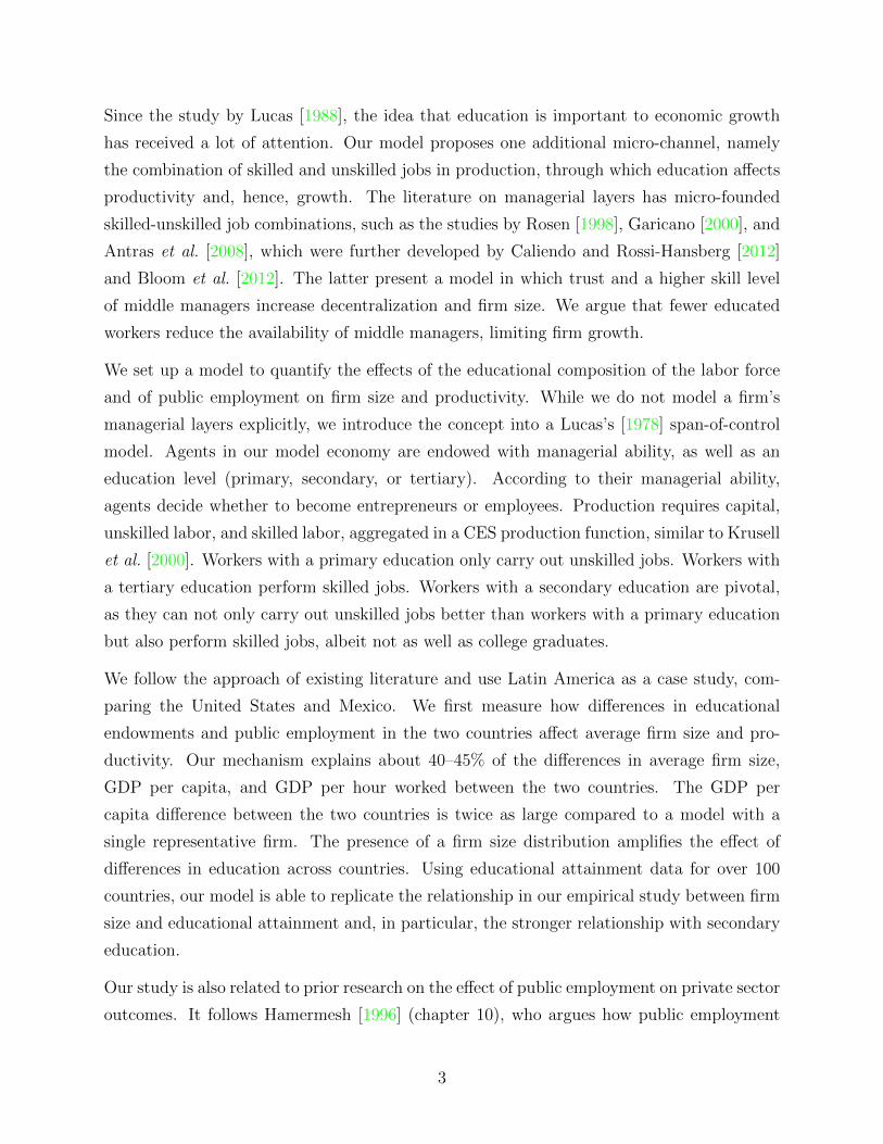
Since the study by Lucas [1988], the idea that education is important to economic growth

has received a lot of attention. Our model proposes one additional micro-channel, namely

the combination of skilled and unskilled jobs in production, through which education affects

productivity and, hence, growth. The literature on managerial layers has micro-founded

skilled-unskilled job combinations, such as the studies by Rosen [1998], Garicano [2000], and

Antras et al. [2008], which were further developed by Caliendo and Rossi-Hansberg [2012]

and Bloom et al. [2012]. The latter present a model in which trust and a higher skill level

of middle managers increase decentralization and firm size. We argue that fewer educated

workers reduce the availability of middle managers, limiting firm growth.

We set up a model to quantify the effects of the educational composition of the labor force

and of public employment on firm size and productivity. While we do not model a firm’s

managerial layers explicitly, we introduce the concept into a Lucas’s [1978] span-of-control

model. Agents in our model economy are endowed with managerial ability, as well as an

education level (primary, secondary, or tertiary). According to their managerial ability,

agents decide whether to become entrepreneurs or employees. Production requires capital,

unskilled labor, and skilled labor, aggregated in a CES production function, similar to Krusell

et al. [2000]. Workers with a primary education only carry out unskilled jobs. Workers with

a tertiary education perform skilled jobs. Workers with a secondary education are pivotal,

as they can not only carry out unskilled jobs better than workers with a primary education

but also perform skilled jobs, albeit not as well as college graduates.

We follow the approach of existing literature and use Latin America as a case study, com-

paring the United States and Mexico. We first measure how differences in educational

endowments and public employment in the two countries affect average firm size and pro-

ductivity. Our mechanism explains about 40–45% of the differences in average firm size,

GDP per capita, and GDP per hour worked between the two countries. The GDP per

capita difference between the two countries is twice as large compared to a model with a

single representative firm. The presence of a firm size distribution amplifies the effect of

differences in education across countries. Using educational attainment data for over 100

countries, our model is able to replicate the relationship in our empirical study between firm

size and educational attainment and, in particular, the stronger relationship with secondary

education.

Our study is also related to prior research on the effect of public employment on private sector

outcomes. It follows Hamermesh [1996] (chapter 10), who argues how public employment

3

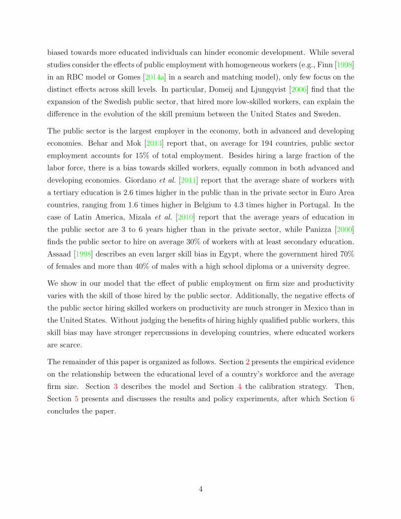
biased towards more educated individuals can hinder economic development. While several

studies consider the effects of public employment with homogeneous workers (e.g., Finn [1998]

in an RBC model or Gomes [2014a] in a search and matching model), only few focus on the

distinct effects across skill levels. In particular, Domeij and Ljungqvist [2006] find that the

expansion of the Swedish public sector, that hired more low-skilled workers, can explain the

difference in the evolution of the skill premium between the United States and Sweden.

The public sector is the largest employer in the economy, both in advanced and developing

economies. Behar and Mok [2013] report that, on average for 194 countries, public sector

employment accounts for 15% of total employment. Besides hiring a large fraction of the

labor force, there is a bias towards skilled workers, equally common in both advanced and

developing economies. Giordano et al. [2011] report that the average share of workers with

a tertiary education is 2.6 times higher in the public than in the private sector in Euro Area

countries, ranging from 1.6 times higher in Belgium to 4.3 times higher in Portugal. In the

case of Latin America, Mizala et al. [2010] report that the average years of education in

the public sector are 3 to 6 years higher than in the private sector, while Panizza [2000]

finds the public sector to hire on average 30% of workers with at least secondary education.

Assaad [1998] describes an even larger skill bias in Egypt, where the government hired 70%

of females and more than 40% of males with a high school diploma or a university degree.

We show in our model that the effect of public employment on firm size and productivity

varies with the skill of those hired by the public sector. Additionally, the negative effects of

the public sector hiring skilled workers on productivity are much stronger in Mexico than in

the United States. Without judging the benefits of hiring highly qualified public workers, this

skill bias may have stronger repercussions in developing countries, where educated workers

are scarce.

The remainder of this paper is organized as follows. Section 2 presents the empirical evidence

on the relationship between the educational level of a country’s workforce and the average

firm size. Section 3 describes the model and Section 4 the calibration strategy. Then,

Section 5 presents and discusses the results and policy experiments, after which Section 6

concludes the paper.

4

2 Firm size distribution and educational attainment

We investigate the relationship between education and firm size using data from the Enter-

prise Survey from the World Bank. The Enterprise Survey has gathered data on 130,000

non-agricultural firms in 135 emerging markets and developing economies since 2002. Note

that firms with fewer than five employees are not surveyed.

Using the full micro data sample, we run a regression of the log of the firm size on age, sec-

tor dummies, time dummies, and country dummies. We then regress the estimated country

dummies on educational attainment. We consider two measures of educational attainment:

completed secondary education and some college, and completed tertiary education. Ac-

cording to Poschke [2011], there is a strong relationship between the average firm size in a

country and its income per capita. We therefore control for the log of GDP per capita and

the log of the population size. Data on the population and GDP per capita comes from the

Penn World Tables and data on educational attainment from the Barro-Lee dataset. As a

robustness check, we use data from the Global Entrepreneurship Monitor survey, which was

Table 2.1: Average employment per firm and educational attainment

Enterprise survey GEM survey

(1) (2) (3) (1) (2) (3)

Income per capita -0.016 0.101** -0.007 0.303** 0.454*** 0.296**

(-0.33) (2.04) (-0.24) (3.22) (3.22) (2.10)

Population 0.089*** 0.089*** 0.085*** -0.056 -0.050 -0.059

(3.10) (2.85) (2.89) (-1.16) (-0.96) (-1.20)

Secondary education 1.202*** 1.217**

(2.80) (2.17)

Tertiary education 0.109 -0.091

(0.11) (-0.07)

Secondary plus 0.853*** 0.837*

tertiary education (3.15) (1.75)

Observations 97 97 97 44 44 44

R-squared 0.251 0.135 0.218 0.413 0.344 0.391Notes: Data on educational attainment of the population over the age of 25 is taken from the Barro-Leedataset for 2005. Tertiary education refers to the fraction of the population that has a college degree.Secondary education refers to the fraction of the population that has completed high school but does nothold a college degree. Data on population and income per capita is taken from the Penn World Tables.For the Enterprise survey, we run a regression of the log of the firm size on the firm’s age, sectordummies, year dummies, and country dummies. The data in the sample refers to the period 2002 to2012. We then regress the country dummies on the log of the population size, the log of the income percapita, and the level of education. For the Global Entrepreneurship Monitor survey, we use the log ofthe country’s average firm employment, as calculated by Poschke [2011]. The t-statistics are shown inbrackets.*** indicates significance at the 1% level, ** indicates significance at 5% level, and * indicatessignificance at the 1% level.

5

conducted in more than 50 countries. In this dataset, we cannot control for sector or age

of the firm, so we use data on the average firm size, as calculated by Poschke [2011] for the

period 2001–2005. The results are shown in Table 2.1.

Perhaps surprisingly, the average firm size is positively related with the fraction of the

population who completed their secondary education, but not with the fraction of college

graduates. The coefficient of secondary education is statistically significant, even when

controlling for GDP per capita, and has a similar magnitude in both surveys. This suggests

that for average firm size, what matters most is the pool of workers with an intermediate

level of education (i.e., completed secondary education or some college). While in advanced

economies, workers with an intermediate education perform unskilled jobs, in developing

countries, they already take on skilled jobs. This flexibility makes them pivotal and more

important in determining firm size than the number of college graduates.

3 Model

We build a model economy a la Lucas [1978], comprising a single representative household

and a government. The household is made up of a continuum of members with different

managerial abilities. According to their managerial abilities, household members become

either employees or entrepreneurs. There are three types of employees in the economy: a

fraction, p, of individuals has primary education, a fraction, s, has completed secondary edu-

cation, and a fraction, t, has completed tertiary education, with p+s+ t = 1. Entrepreneurs

produce a homogeneous good by using unskilled labor, skilled labor, capital, and their ability

as inputs. A household decides on levels of consumption and savings given the joint income

of the household members.

Household The household is composed of a continuum of members. Its total size is

normalized to unity. The household maximizes the infinite sum of discounted utilities given

by∞∑t=0

βtlog(Ct), (3.1)

where Ct denotes total household consumption at time t and β ∈ (0, 1) is the discount factor.

Since we focus on the steady state and for expositional clarity, we omit the time subscript,

t, from the description of the model.

6

Endowments Each household member has one unit of productive time that he/she sup-

plies inelastically. Household members differ in their level of education and managerial

abilities, zi, distributed in Z = [0, z], with cdf F (zi) and density f(zi). The household

assigns occupations to its members depending on their abilities and education. They can

become either workers or entrepreneurs.

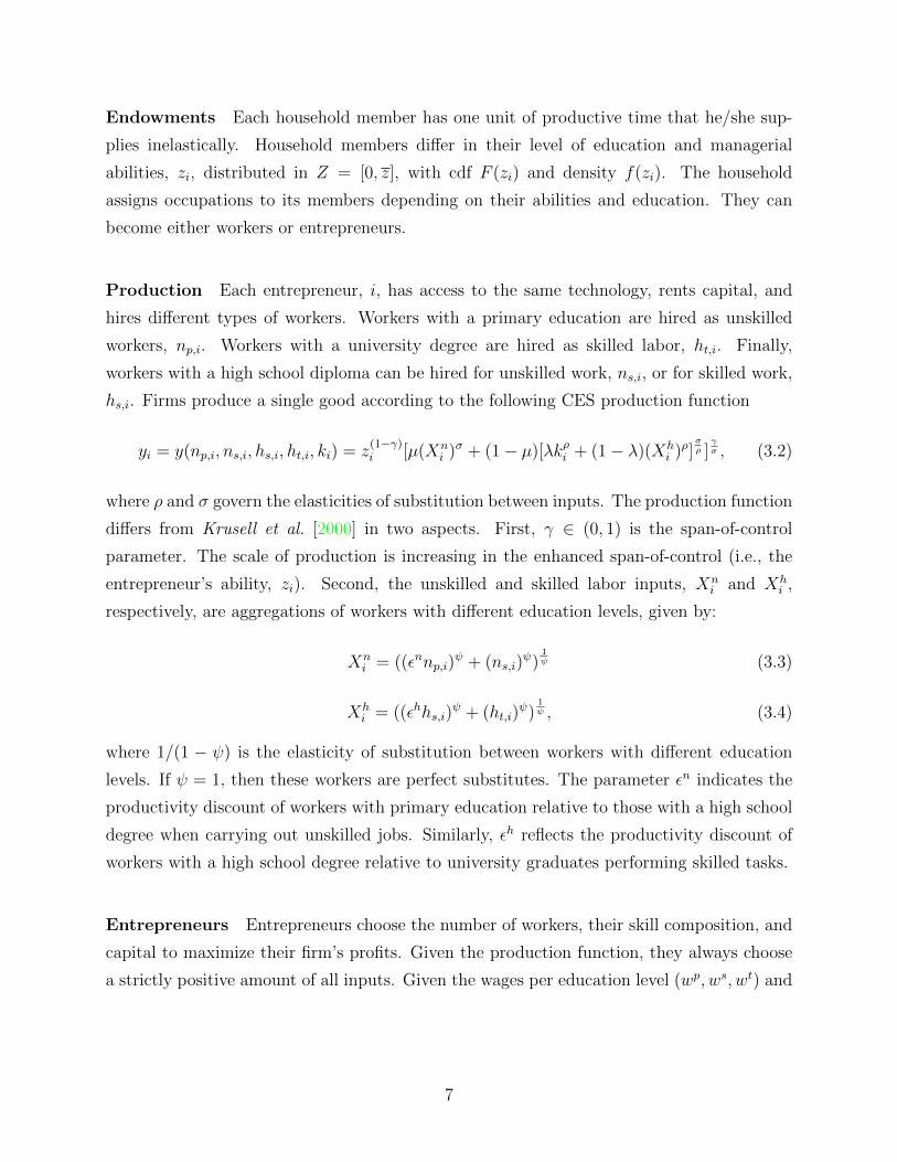
Production Each entrepreneur, i, has access to the same technology, rents capital, and

hires different types of workers. Workers with a primary education are hired as unskilled

workers, np,i. Workers with a university degree are hired as skilled labor, ht,i. Finally,

workers with a high school diploma can be hired for unskilled work, ns,i, or for skilled work,

hs,i. Firms produce a single good according to the following CES production function

yi = y(np,i, ns,i, hs,i, ht,i, ki) = z(1−γ)i [µ(Xn

i )σ + (1− µ)[λkρi + (1− λ)(Xhi )ρ]

σρ ]

γσ , (3.2)

where ρ and σ govern the elasticities of substitution between inputs. The production function

differs from Krusell et al. [2000] in two aspects. First, γ ∈ (0, 1) is the span-of-control

parameter. The scale of production is increasing in the enhanced span-of-control (i.e., the

entrepreneur’s ability, zi). Second, the unskilled and skilled labor inputs, Xni and Xh

i ,

respectively, are aggregations of workers with different education levels, given by:

Xni = ((εnnp,i)

ψ + (ns,i)ψ)

1ψ (3.3)

Xhi = ((εhhs,i)

ψ + (ht,i)ψ)

1ψ , (3.4)

where 1/(1 − ψ) is the elasticity of substitution between workers with different education

levels. If ψ = 1, then these workers are perfect substitutes. The parameter εn indicates the

productivity discount of workers with primary education relative to those with a high school

degree when carrying out unskilled jobs. Similarly, εh reflects the productivity discount of

workers with a high school degree relative to university graduates performing skilled tasks.

Entrepreneurs Entrepreneurs choose the number of workers, their skill composition, and

capital to maximize their firm’s profits. Given the production function, they always choose

a strictly positive amount of all inputs. Given the wages per education level (wp, ws, wt) and

7

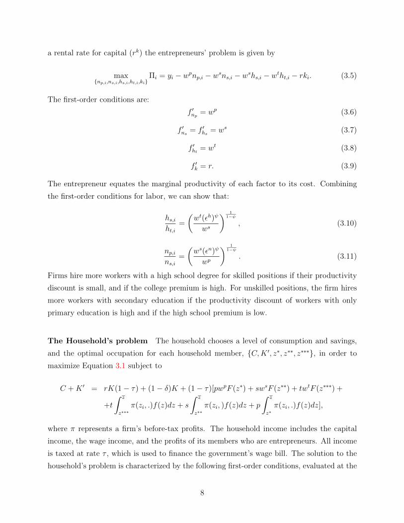
a rental rate for capital (rk) the entrepreneurs’ problem is given by

max{np,i,ns,i,hs,i,ht,i,ki}

Πi = yi − wpnp,i − wsns,i − wshs,i − wtht,i − rki. (3.5)

The first-order conditions are:

f ′np = wp (3.6)

f ′ns = f ′hs = ws (3.7)

f ′ht = wt (3.8)

f ′k = r. (3.9)

The entrepreneur equates the marginal productivity of each factor to its cost. Combining

the first-order conditions for labor, we can show that:

hs,iht,i

=

(wt(εh)ψ

ws

) 11−ψ

, (3.10)

np,ins,i

=

(ws(εn)ψ

wp

) 11−ψ

. (3.11)

Firms hire more workers with a high school degree for skilled positions if their productivity

discount is small, and if the college premium is high. For unskilled positions, the firm hires

more workers with secondary education if the productivity discount of workers with only

primary education is high and if the high school premium is low.

The Household’s problem The household chooses a level of consumption and savings,

and the optimal occupation for each household member, {C,K ′, z∗, z∗∗, z∗∗∗}, in order to

maximize Equation 3.1 subject to

C +K ′ = rK(1− τ) + (1− δ)K + (1− τ)[pwpF (z∗) + swsF (z∗∗) + twtF (z∗∗∗) +

+t

∫ z

z∗∗∗π(zi, .)f(z)dz + s

∫ z

z∗∗π(zi, )f(z)dz + p

∫ z

z∗π(zi, .)f(z)dz],

where π represents a firm’s before-tax profits. The household income includes the capital

income, the wage income, and the profits of its members who are entrepreneurs. All income

is taxed at rate τ , which is used to finance the government’s wage bill. The solution to the

household’s problem is characterized by the following first-order conditions, evaluated at the

8

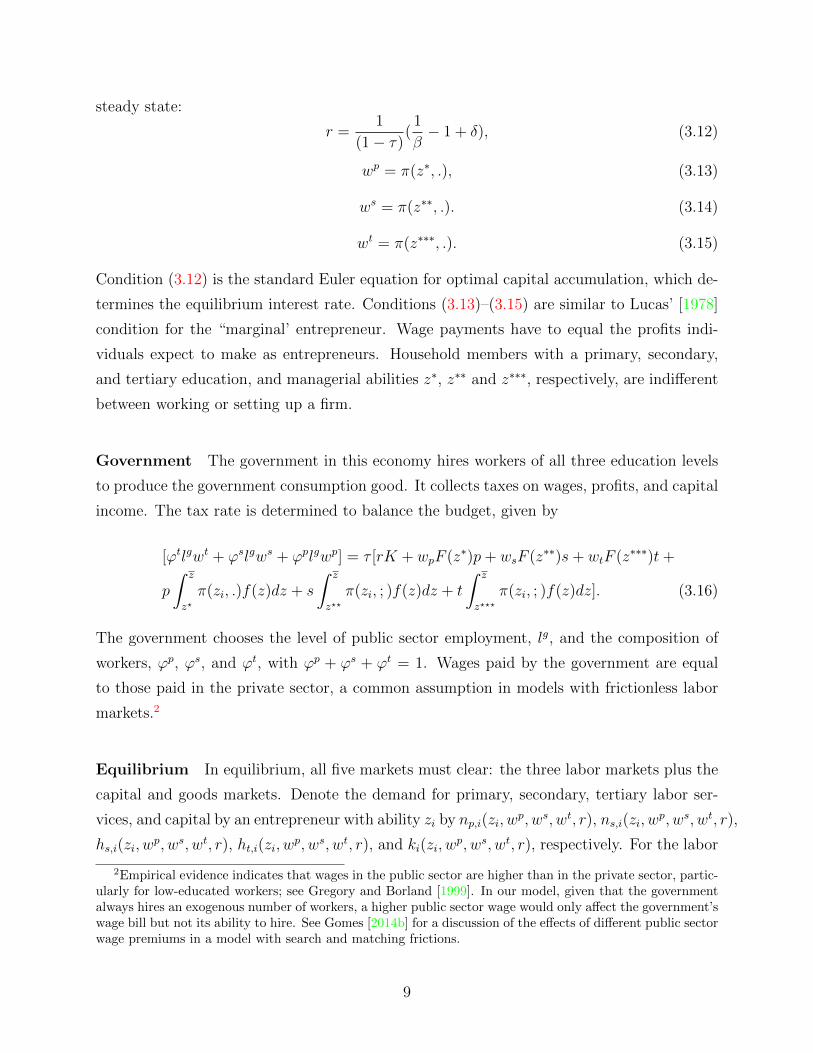
steady state:

r =1

(1− τ)(1

β− 1 + δ), (3.12)

wp = π(z∗, .), (3.13)

ws = π(z∗∗, .). (3.14)

wt = π(z∗∗∗, .). (3.15)

Condition (3.12) is the standard Euler equation for optimal capital accumulation, which de-

termines the equilibrium interest rate. Conditions (3.13)–(3.15) are similar to Lucas’ [1978]

condition for the “marginal’ entrepreneur. Wage payments have to equal the profits indi-

viduals expect to make as entrepreneurs. Household members with a primary, secondary,

and tertiary education, and managerial abilities z∗, z∗∗ and z∗∗∗, respectively, are indifferent

between working or setting up a firm.

Government The government in this economy hires workers of all three education levels

to produce the government consumption good. It collects taxes on wages, profits, and capital

income. The tax rate is determined to balance the budget, given by

[ϕtlgwt + ϕslgws + ϕplgwp] = τ [rK + wpF (z∗)p+ wsF (z∗∗)s+ wtF (z∗∗∗)t+

p

∫ z

z?π(zi, .)f(z)dz + s

∫ z

z??π(zi, ; )f(z)dz + t

∫ z

z???π(zi, ; )f(z)dz]. (3.16)

The government chooses the level of public sector employment, lg, and the composition of

workers, ϕp, ϕs, and ϕt, with ϕp + ϕs + ϕt = 1. Wages paid by the government are equal

to those paid in the private sector, a common assumption in models with frictionless labor

markets.2

Equilibrium In equilibrium, all five markets must clear: the three labor markets plus the

capital and goods markets. Denote the demand for primary, secondary, tertiary labor ser-

vices, and capital by an entrepreneur with ability zi by np,i(zi, wp, ws, wt, r), ns,i(zi, w

p, ws, wt, r),

hs,i(zi, wp, ws, wt, r), ht,i(zi, w

p, ws, wt, r), and ki(zi, wp, ws, wt, r), respectively. For the labor

2Empirical evidence indicates that wages in the public sector are higher than in the private sector, partic-ularly for low-educated workers; see Gregory and Borland [1999]. In our model, given that the governmentalways hires an exogenous number of workers, a higher public sector wage would only affect the government’swage bill but not its ability to hire. See Gomes [2014b] for a discussion of the effects of different public sectorwage premiums in a model with search and matching frictions.

9

market to clear:

P ≡ F (z∗)p = ϕplg + p

∫ z

z∗np,i(zi, w

p, ws, wt, r)f(z)dz + s

∫ z

z∗∗np,i(zi, w

p, ws, wt, r)f(z)dz

+t

∫ z

z∗∗∗np,i(zi, w

p, ws, wt, r)f(z)dz. (3.17)

The aggregate supply of workers with primary education, P , must equal the sum of labor

demands by all entrepreneurs and the government. For workers with a secondary and tertiary

education, the labor market clears when:

S ≡ F (z∗)s = ϕslg + p

∫ z

z∗ns,i(zi, w

p, ws, wt, r)f(z)dz + p

∫ z

z∗hs,i(zi, w

p, ws, wt, r)f(z)dz

+s

∫ z

z∗∗ns,i(zi, w

p, ws, wt, r)f(z)dz + s

∫ z

z∗∗hs,i(zi, w

p, ws, wt, r)f(z)dz +

t

∫ z

z∗∗∗ns,i(zi, w

p, ws, wt, r)f(z)dz + t

∫ z

z∗∗∗hs,i(zi, w

p, ws, wt, r)f(z)dz.(3.18)

and

T ≡ F (z∗∗∗)t = ϕtlg + p

∫ z

z∗ht,i(zi, w

p, ws, wt, r)f(z)dz + s

∫ z

z∗∗ht,i(zi, w

p, ws, wt, r)f(z)dz

+t

∫ z

z∗∗∗ht,i(zi, w

p, ws, wt, r)f(z)dz. (3.19)

The market clearing condition for capital is given by:

K = p

∫ z

z∗ki(zi, w

p, ws, wt, r)f(z)dz + s

∫ z

z∗∗ki(zi, w

p, ws, wt, r)f(z)dz

+t

∫ z

z∗∗∗ki(zi, w

p, ws, wt, r)f(z)dz. (3.20)

With yi(zi, wp, ws, wt, r) being the supply of goods by any entrepreneur of ability zi, for

market clearing in the goods market, we require

p

∫ z

z∗yi(zi, w

p, ws, wt, r)f(z)dz + s

∫ z

z∗∗yi(zi, w

p, ws, wt, r)f(z)dz

+ t

∫ z

z∗∗∗yi(zi, w

p, ws, wt, r)f(z)dz = C + δK. (3.21)

We can now define a competitive equilibrium for the model economy in the steady state.

10

Given a government policy {lg, ϕp, ϕs, ϕg} and a sequence of prices for labor and capital

{wp, ws, wt, r}, a competitive equilibrium is a collection of thresholds {z∗, z∗∗, z∗∗∗}, a tax

rate {τ}, and allocations {P, S, T,K ′, C}, such that:

1. {z∗, z∗∗, z∗∗∗} solve the household’s problem (i.e., equations (3.13)–(3.15) hold) ;

2. the rental rate is determined by the Euler equation (3.12);

3. the five markets for goods, capital, primary, secondary, and tertiary labor all clear (i.e.,

equations (3.17)–(3.21) hold);

4. the tax rate, τ , balances the government’s budget (i.e., equation (3.16) holds).

In order to illustrate the main mechanism of the model, we show how potential entrepreneurs

of any talent would adjust their input choices when faced with different factor prices. Figure

3.1 shows these adjustments when entrepreneurs face higher college or high school premiums.

When tertiary wages are high (gray line), entrepreneurs substitute away from workers with

a university degree and hire more workers with a secondary education to perform skilled

jobs. The productivity of those workers in skilled positions is lower, and firms thus hire

fewer unskilled workers and use less capital. Overall, for each level of entrepreneurial ability,

Figure 3.1: Sizes of firms, for different college and high school premiums

Terciary workers

Managerial ability

Un

its

BaselineLarger college premiumLarger high−school premium

Secundary workers (skilled)

Managerial ability

Un

its

BaselineLarger college premiumLarger high−school premium

Secundary workers (unskilled)

Managerial ability

Un

its

BaselineLarger college premiumLarger high−school premium

Primary workers

Managerial ability

Un

its

BaselineLarger college premiumLarger high−school premium

Total workers

Managerial ability

Un

its

BaselineLarger college premiumLarger high−school premium

Capital

Managerial ability

Un

its

BaselineLarger college premiumLarger high−school premium

11

firms will be smaller. When the wages of workers with a secondary education are higher

(dark line), firms substitute away from these workers towards college graduates to perform

skilled jobs, and towards workers with a primary education for unskilled jobs. Workers with

a primary education are less productive in unskilled positions; hence, firms use less capital

and operate on a smaller scale.

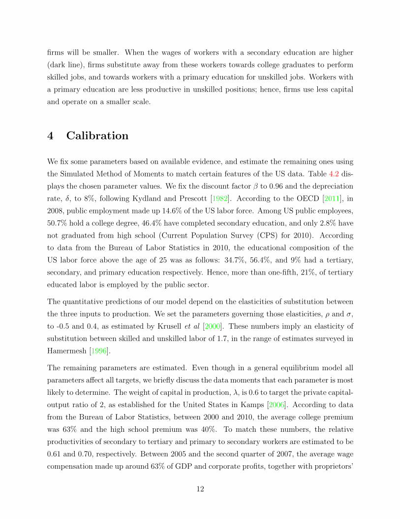
4 Calibration

We fix some parameters based on available evidence, and estimate the remaining ones using

the Simulated Method of Moments to match certain features of the US data. Table 4.2 dis-

plays the chosen parameter values. We fix the discount factor β to 0.96 and the depreciation

rate, δ, to 8%, following Kydland and Prescott [1982]. According to the OECD [2011], in

2008, public employment made up 14.6% of the US labor force. Among US public employees,

50.7% hold a college degree, 46.4% have completed secondary education, and only 2.8% have

not graduated from high school (Current Population Survey (CPS) for 2010). According

to data from the Bureau of Labor Statistics in 2010, the educational composition of the

US labor force above the age of 25 was as follows: 34.7%, 56.4%, and 9% had a tertiary,

secondary, and primary education respectively. Hence, more than one-fifth, 21%, of tertiary

educated labor is employed by the public sector.

The quantitative predictions of our model depend on the elasticities of substitution between

the three inputs to production. We set the parameters governing those elasticities, ρ and σ,

to -0.5 and 0.4, as estimated by Krusell et al [2000]. These numbers imply an elasticity of

substitution between skilled and unskilled labor of 1.7, in the range of estimates surveyed in

Hamermesh [1996].

The remaining parameters are estimated. Even though in a general equilibrium model all

parameters affect all targets, we briefly discuss the data moments that each parameter is most

likely to determine. The weight of capital in production, λ, is 0.6 to target the private capital-

output ratio of 2, as established for the United States in Kamps [2006]. According to data

from the Bureau of Labor Statistics, between 2000 and 2010, the average college premium

was 63% and the high school premium was 40%. To match these numbers, the relative

productivities of secondary to tertiary and primary to secondary workers are estimated to be

0.61 and 0.70, respectively. Between 2005 and the second quarter of 2007, the average wage

compensation made up around 63% of GDP and corporate profits, together with proprietors’

12

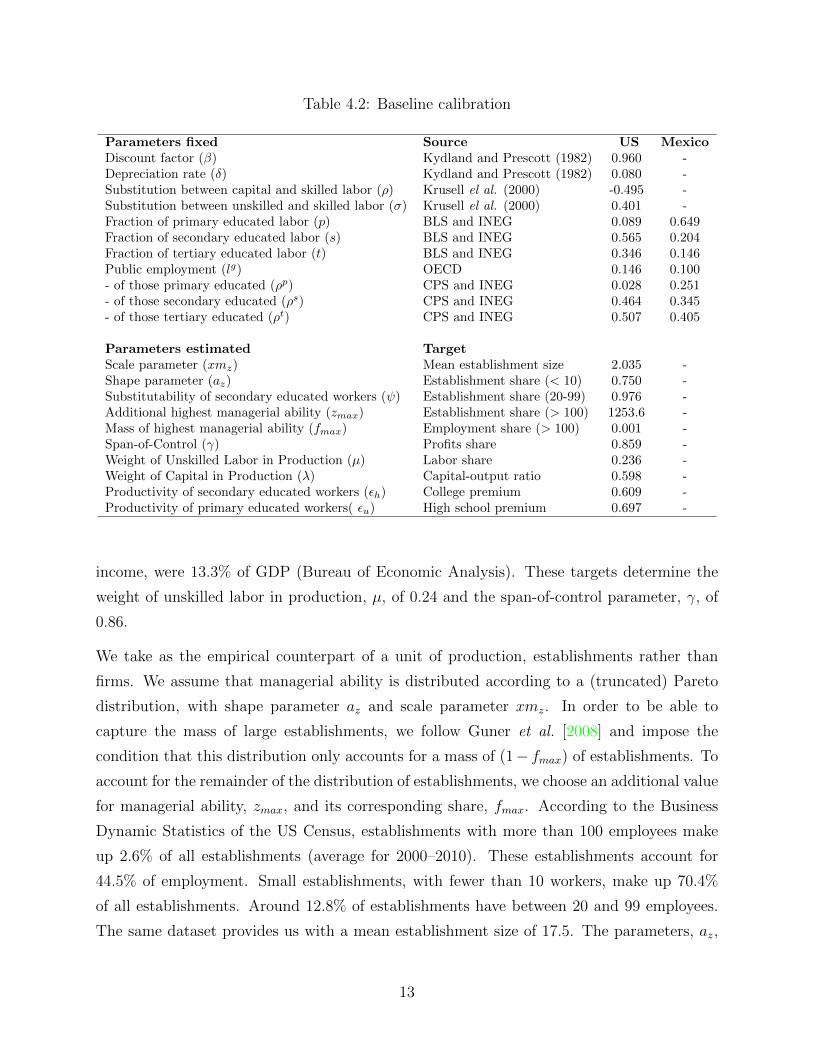
Table 4.2: Baseline calibration

Parameters fixed Source US MexicoDiscount factor (β) Kydland and Prescott (1982) 0.960 -Depreciation rate (δ) Kydland and Prescott (1982) 0.080 -Substitution between capital and skilled labor (ρ) Krusell el al. (2000) -0.495 -Substitution between unskilled and skilled labor (σ) Krusell el al. (2000) 0.401 -Fraction of primary educated labor (p) BLS and INEG 0.089 0.649Fraction of secondary educated labor (s) BLS and INEG 0.565 0.204Fraction of tertiary educated labor (t) BLS and INEG 0.346 0.146Public employment (lg) OECD 0.146 0.100- of those primary educated (ρp) CPS and INEG 0.028 0.251- of those secondary educated (ρs) CPS and INEG 0.464 0.345- of those tertiary educated (ρt) CPS and INEG 0.507 0.405

Parameters estimated TargetScale parameter (xmz) Mean establishment size 2.035 -Shape parameter (az) Establishment share (< 10) 0.750 -Substitutability of secondary educated workers (ψ) Establishment share (20-99) 0.976 -Additional highest managerial ability (zmax) Establishment share (> 100) 1253.6 -Mass of highest managerial ability (fmax) Employment share (> 100) 0.001 -Span-of-Control (γ) Profits share 0.859 -Weight of Unskilled Labor in Production (µ) Labor share 0.236 -Weight of Capital in Production (λ) Capital-output ratio 0.598 -Productivity of secondary educated workers (εh) College premium 0.609 -Productivity of primary educated workers( εu) High school premium 0.697 -

income, were 13.3% of GDP (Bureau of Economic Analysis). These targets determine the

weight of unskilled labor in production, µ, of 0.24 and the span-of-control parameter, γ, of

0.86.

We take as the empirical counterpart of a unit of production, establishments rather than

firms. We assume that managerial ability is distributed according to a (truncated) Pareto

distribution, with shape parameter az and scale parameter xmz. In order to be able to

capture the mass of large establishments, we follow Guner et al. [2008] and impose the

condition that this distribution only accounts for a mass of (1− fmax) of establishments. To

account for the remainder of the distribution of establishments, we choose an additional value

for managerial ability, zmax, and its corresponding share, fmax. According to the Business

Dynamic Statistics of the US Census, establishments with more than 100 employees make

up 2.6% of all establishments (average for 2000–2010). These establishments account for

44.5% of employment. Small establishments, with fewer than 10 workers, make up 70.4%

of all establishments. Around 12.8% of establishments have between 20 and 99 employees.

The same dataset provides us with a mean establishment size of 17.5. The parameters, az,

13

Table 4.3: Calibration targets and model values

Targeted moments Source Data ModelMean establishment size US Census 17.46 17.46Establishment share, < 10 employees US Census 0.704 0.700Establishment share, 20-99 employees US Census 0.128 0.104Establishment share, > 100 employees US Census 0.026 0.025Employment share, > 100 employees US Census 0.445 0.434Capital-output-ratio Kamps (2006) 2.000 1.997Profits to GDP BEA 0.133 0.127Wage bill BEA 0.630 0.603College Premium BLS 0.630 0.630High School Premium BLS 0.400 0.400

Not targeted moments SourceEmployment share, < 10 employees US Census 0.146 0.195Employment share, 20-99 employees US Census 0.297 0.232Self-employment rate OECD 0.071 0.046Self-employment rate, adjusted US Census 0.018 0.046

xmz, zmax, fmax, and ψ are estimated to be 0.75, 2.03, 1253.6, 0.001, and 0.98, respectively.

Note that ψ is close to unity, implying a high substitutability between workers with different

levels of education performing the same type of job.

Our model matches the data well. Table 4.3 displays the calibration targets next to the

model values, as well as some additional moments that were not targeted. The model

somewhat underestimates the labor share of the economy, as well as the fraction of mid-size

establishments.3 On the other hand, the model somewhat overestimates the employment

share of small establishments, while underestimating that of mid-size establishments. There

are also fewer entrepreneurs in the model compared to the data. According to OECD

statistics, 7.05% of the US labor force was self-employed in 2010, while in the model, only

4.63% of individuals set up a firm. This difference is partly because the model only considers

firms with at least one employee. However, around 75% of businesses in the United States

are non-employers (US census). Adjusting the self-employment rate for this number would

result in a low 1.76% of the labor force owning a firm with employees, which is clearly smaller

than the model’s statistic. While each firm in the model has one entrepreneur, in the data,

one entrepreneur is likely to own various firms.

To evaluate the impact of the supply of skilled labor, we compare our benchmark economy to

an identical economy, but using the educational attainment and public employment policy of

3This seems to be a problem of the Pareto distribution, while the common alternative—the log-normaldistribution—performs worse in the upper tail of the distribution. For more information, see Coad [2009].

14

Mexico. The data for Mexico come from the Encuesta Nacional de Ocupacion y Empleo of the

Instituto Nacional de Estadistica y Geografıa (INEG), available for the 3rd and 4th quarter of

2010. Around 15% of the Mexican labor force held a college degree, 20% had completed their

secondary education, and 65% had, at most, received an incomplete secondary education.4

According to the OECD [2011], in 2008, Mexico’s public sector (public administration or

publicly owned firms) hired 10% of the labor force. Among public employees, more than

40% held a college degree, while only 25% had not completed secondary education. These

numbers are shown in the last column of Table 4.2.

5 Results

5.1 United States versus Mexico

The level of education of the Mexican labor force is much lower than that of the US labor

force. Even though Mexico has one of the smallest public sectors among OECD countries,

public employment is clearly biased towards skilled individuals. More than one-fourth, 28%,

of all employees with a tertiary education work in the public sector. The absorption of skilled

labor by the public sector is thus more acute in Mexico than in the United States. What

does this imply for the private sector and, in particular, for firm size and productivity?

Table 5.4 displays the benchmark results for the United States next to those for Mexico.

For Mexico, we show the results for a case in which the tax rate adjusts to keep the budget

balanced and another one where the government uses lump-sum taxes. In our model, the

mean firm size in Mexico is lower than in the US, where the average Mexican firm has five

fewer workers compared to the average US firm. Given the observed size of US (17.46) and

Mexican firms (5.4 workers, see INEG [2014]), our model can explain around 41% of the

difference.Firms in Mexico operate on a smaller scale and also use less capital. This leads

to a low capital-output ratio of 1.65. McGrattan and Smith [1999] estimate the US capital-

output ratio to be 1.32 times that of Mexico. In our model, the private capital-output ratio

in the United States is 1.2 times that of Mexico, accounting for 63% of the relative difference.

Capital costs in our model are the same in the United States and Mexico (in column 3,

4The fraction of those with a tertiary education is similar to that in Machin and McNally [2007] for thepopulation aged 25–64 in 2003, but higher than that in Barceinas [2005] for the population aged 15 andabove in 2000.

15

Table 5.4: Results: United States and Mexico

United States MexicoVariables No tax adjustment Tax adjustedMean establishment size 17.46 12.45 12.45Establishment share, < 10 employees 0.70 0.80 0.80Establishment share, 20-99 employees 0.10 0.07 0.07Establishment share, > 100 employees 0.03 0.02 0.02Employment share, > 100 employees 0.43 0.44 0.44Capital-output-ratio 2.00 1.66 1.64Profits to GDP 0.13 0.12 0.12Labor share 0.60 0.65 0.65College premium 0.63 0.64 0.64High school premium 0.40 2.71 2.68Tax Rate 0.10 0.10 0.12

Productivity measuresEntrepreneurs 0.05 0.07 0.07Average managerial talent 100 71.85 71.84Output per establishment 100 46.58 46.35Employment by largest establishments 100 99.27 99.24Private sector output per worker 100 65.31 (78.2) 65.02 (77.9)Private sector output per capita 100 67.36 (82.3) 67.05 (82.1)GDP per worker 100 70.12 (86.5) 69.78 (86.1)GDP per capita 100 68.61 (86.5) 68.27 (86.1)

Notes: result of model simulations. In brackets are the results from a model with a representative firmwith constant returns to scale (γ = 1), under the same calibration.

they only differ slightly due to higher taxes). It is the higher skill premiums in Mexico that

drive the differences in firms’ input choices. The skill premium for those with a tertiary, but

especially secondary education is much higher in Mexico; more than six times the one in the

United States. This is high, but it is qualitatively in line with empirical evidence. According

to Lopez-Acevedo [2001], workers with a college degree in Mexico earn 53% more than those

with an upper secondary education, who in turn earn 70% more than those with a primary

education and 170% more than those with no schooling. In contrast to the United States,

in Mexico there is a larger relative difference in wages between those with a primary and

secondary education than between those with a secondary and tertiary education.

Productivity in Mexico is lower when comparing all measures. In line with OECD data,

more individuals in Mexico set up firms than in the United States. More entrepreneurs

implies lower average managerial talent. More managers of lower talent who produce with

less capital and on smaller scales leads to lower private output per worker. GDP—the sum of

private output and the government’s wage bill—is also lower. According to OECD statistics,

GDP per capita (current PPP adjusted US$) in Mexico in 2010 was around 31% of that in

16

the United States. In our model, Mexican GDP per capita is equal to 69% of US GDP,

accounting for around 45% of the observed difference. Similarly, our mechanism is able

to capture around 46% of the difference in workers’ productivity, measured as GDP per

worker/per hours worked.

A model with a representative firm would also generate differences in GDP per capita, be-

cause of the lower educational attainment in Mexico. To quantify how much the distribution

of firms can amplify these differences, we compute the productivity measures in a model

with a representative firm and constant returns to scale in production. In the model with

firm size distribution, the relative GDP per capita between the United States and Mexico is

twice as high compared to the model with a representative firm.

5.2 Cross-country analysis

Using data on educational attainment for all countries from the Barro-Lee dataset, we test

how well the model is able to replicate the positive cross-country relationship between edu-

cational attainment and average firm size. We assume that the government hires 21% of all

college graduates and 12% of all high school graduates, the same fractions as in the United

States. The hiring of workers with primary education is such that the overall level of public

employment is 14.6%, as in the United States.

The first chart of Figure 5.2 shows the positive relationship between secondary educational

attainment and average firm size. The slope of the regression is close to 0.76, compared

Figure 5.2: Mean firm size and educational attainment in model

Mexico

United States

ln(size) = 2.38 + 0.76 s, R2=0.80(24.4)

ln(size) = 2.37 + 0.66 s + 0.39 t, R2=0.82(17.2) (3.9)

2.4

2.5

2.6

2.7

2.8

2.9

Mod

el fi

rm s

ize

(logs

)

0 20 40 60 80% population with secundary education completed

United States

Mexicoln(size) = 2.48 + 1.48 t, R2=0.46

ln(size) = 2.37 + 0.66 s + 0.39 t, R2=0.82

(11.1)

(17.2) (3.9)

2.4

2.5

2.6

2.7

2.8

2.9

Mod

el fi

rm s

ize

(logs

)

0 10 20 30 40% population with tertiary education completed

Data: Educational Attainment: Barro-Lee dataset; Firm size: Model

17

to 1.2 found in Section 2, confirming that secondary education plays a crucial role for firm

size. The R-squared is 0.80. Adding the fraction of those with a tertiary education to the

regression of the log of the firm size on secondary education marginal raises the R-squared to

0.82, suggesting a limited contribution of tertiary education to firm size. The second chart

confirms this, showing much more dispersion in the relationship between tertiary education

and firm size.

5.3 Increase in public employment

We run a policy experiment that increases public employment in the United States and Mex-

ico by five percentage points, financed by lump-sum taxes. We test three different scenarios

for hiring additional workers: (i) only hiring those with a tertiary education, (ii) only hir-

ing those with a secondary education, and (iii) only hiring those with a primary education.

Table 5.5 displays the percentage variation in the model’s moments compared to the re-

spective benchmark for the United States and Mexico. Additional public employment offers

an attractive outside option to setting up a firm. Fewer individuals become entrepreneurs.

The average managerial talent increases and the labor share of the economy increases, while

profits to GDP fall. Less private output is produced, and even as more production takes

place within the public sector, GDP per capita and GDP per worker fall. Less employment

is concentrated in the most productive firms. Lastly, smaller large firms and a larger public

sector that does not use capital leads to a lower capital-output ratio.

The impacts of public sector hiring are more pronounced in Mexico relative to the United

States, particularly when hiring more educated workers. While hiring college graduates raises

the college premium by 1.7% and the high school premium by 1.1% in the United States, it

raises the same statistics by 4% and 27% in Mexico. In addition, while the US private sector

output per worker falls by 1.4%, that in Mexico falls by 11 percent. The increase in public

employment causes firms to hire fewer skilled employees and to operate on a smaller scale.

Given capital-skill complementarity, fewer skilled workers reduces the capital-output ratio.

A final important conclusion is that the effects of public sector hiring clearly depend on

which type of worker is hired. For instance, in Mexico, if all additional public employees

have a tertiary education, the private sector output per worker falls by 11% and profits by

13%. However, if the additional employees are high school graduates the effects are only 4%

and 8%, respectively. These results do not differ when the increase in public sector hiring is

18

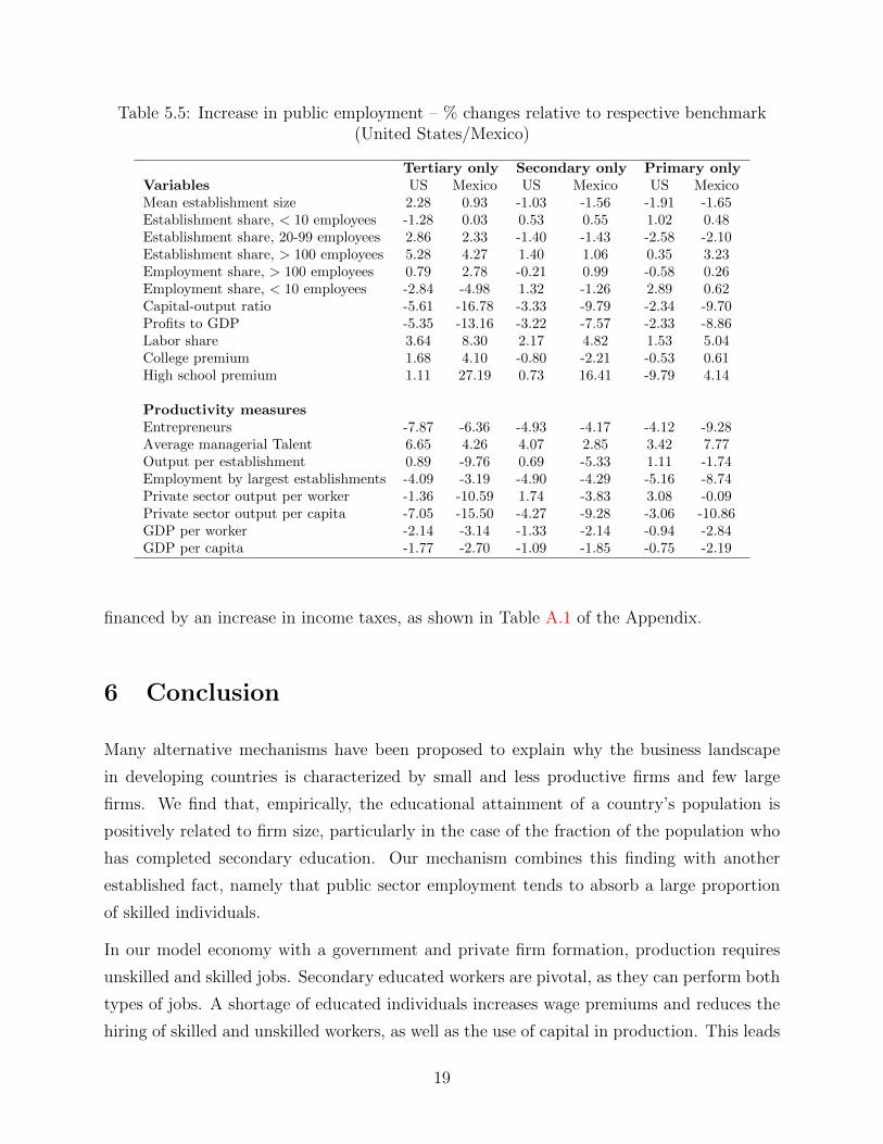
Table 5.5: Increase in public employment – % changes relative to respective benchmark(United States/Mexico)

Tertiary only Secondary only Primary onlyVariables US Mexico US Mexico US MexicoMean establishment size 2.28 0.93 -1.03 -1.56 -1.91 -1.65Establishment share, < 10 employees -1.28 0.03 0.53 0.55 1.02 0.48Establishment share, 20-99 employees 2.86 2.33 -1.40 -1.43 -2.58 -2.10Establishment share, > 100 employees 5.28 4.27 1.40 1.06 0.35 3.23Employment share, > 100 employees 0.79 2.78 -0.21 0.99 -0.58 0.26Employment share, < 10 employees -2.84 -4.98 1.32 -1.26 2.89 0.62Capital-output ratio -5.61 -16.78 -3.33 -9.79 -2.34 -9.70Profits to GDP -5.35 -13.16 -3.22 -7.57 -2.33 -8.86Labor share 3.64 8.30 2.17 4.82 1.53 5.04College premium 1.68 4.10 -0.80 -2.21 -0.53 0.61High school premium 1.11 27.19 0.73 16.41 -9.79 4.14

Productivity measuresEntrepreneurs -7.87 -6.36 -4.93 -4.17 -4.12 -9.28Average managerial Talent 6.65 4.26 4.07 2.85 3.42 7.77Output per establishment 0.89 -9.76 0.69 -5.33 1.11 -1.74Employment by largest establishments -4.09 -3.19 -4.90 -4.29 -5.16 -8.74Private sector output per worker -1.36 -10.59 1.74 -3.83 3.08 -0.09Private sector output per capita -7.05 -15.50 -4.27 -9.28 -3.06 -10.86GDP per worker -2.14 -3.14 -1.33 -2.14 -0.94 -2.84GDP per capita -1.77 -2.70 -1.09 -1.85 -0.75 -2.19

financed by an increase in income taxes, as shown in Table A.1 of the Appendix.

6 Conclusion

Many alternative mechanisms have been proposed to explain why the business landscape

in developing countries is characterized by small and less productive firms and few large

firms. We find that, empirically, the educational attainment of a country’s population is

positively related to firm size, particularly in the case of the fraction of the population who

has completed secondary education. Our mechanism combines this finding with another

established fact, namely that public sector employment tends to absorb a large proportion

of skilled individuals.

In our model economy with a government and private firm formation, production requires

unskilled and skilled jobs. Secondary educated workers are pivotal, as they can perform both

types of jobs. A shortage of educated individuals increases wage premiums and reduces the

hiring of skilled and unskilled workers, as well as the use of capital in production. This leads

19

to smaller and less productive firms. Calibrated to the United States, our model can account

for around 40–45% of the differences in average firm size, GDP per capita, and GDP per

hour worked between the United States and Mexico.

Empirical findings have suggested an important role of secondary education in reducing

income inequality (see Tilak [1989]). Our model proposes a possible micro mechanism of

how a larger fraction of those with a secondary education can lead to higher output, lower

wage premiums, and thus a lower wage inequality. Regarding public policies, we show how

these may unintentionally affect firm size and productivity. In particular, effects may be

different depending on which skill groups are hired by the public sector. Our model thus

allows us to measure the effects of public sector hiring that go beyond those already pointed

out by previous studies, such as queuing or changes in skill premiums.

References

Amaral, Pedro S. and Erwan Quintin (2006): “A Competitive Model of the Infor-mal Sector,” Journal of Monetary Economics, 53 (7), pp. 1541-53.

Antras Pol; Garicano, Luis and Esteban Rossi-Hansberg (2008): “Organiz-ing Offshoring: Middle Managers and Communication Costs,” in The Organization ofFirms in a Global Economy,edited by Helpman, E.m D. Main and T. Verdier. HarvardUniversity Press

Antunes, Antonio R. and Tiago V. de V. Cavalcanti (2007): “Start up costs,limited enforcement and the hidden economy,” European Economic Review , 51 (1), pp.203-224.

Assaad, Ragui (1997): “The effects of public sector hiring and compensation policieson the Egyptian labour market,” The World Bank Economic Review, 11(1) , pp. 85-118.

Barceinas, Fernando (2005): “Educacion y distribucion del ingreso en Mexico”, Sis-tema de Informacion de Tendendicas Educativas en America Latina.

Behar, Alberto and Mok, Junghwan (2013): “Does Public-Sector EmploymentFully Crowd Out Private-Sector Employment?”, IMF Working Paper 13/146.

Bloom, Nick; Sadun, Raffaella and John Van Reenen (2012): “The Organizationof Firms across Countries,” Quarterly Journal of Economics, 127(4), pp. 1663?1705.

Braguinsky, Serguey; Branstetter, Lee G. and Andre Regateiro (2011): “TheIncredible Shrinking Portuguese Firm”, NBER Working Paper No. 17265.

20

Cabral, Luıs M. B. and Jose Mata (2003): “On the Evolution of the Firm SizeDistribution: Facts and Theory,” The American Economic Review, 93 (4), pp. 1075-1090.

Caliendo, Lorenzo and Esteban Rossi-Hansberg (2012): “The Impact of Tradeon Organization and Productivity,” Quarterly Journal of Economics forthcoming.

Chong, Alberto and Mark Gradstein (2007): “Inequality and Informality,” Journalof Public Economics, 91 (1/2), pp. 159-179.

Coad, Alex: The Growth of Firms: A Survey of Theories and Empirical Evidence.New Perspectives on the Modern Corporation, Edward Elgar Pub, 2009.

Davis, Steven J. and Markus Henrekson (1999): “Explaining National Differencesin the Size and Industry Distribution of Employment,” Small Business Economics,12(1), pp. 59-83.

Domeij, David and Lars Ljungqvist (2006): “Wage Structure and Public SectorEmployment: Sweden versus the United States 1970-2002,” Working Paper Series inEconomics and Finance 638, Stockholm School of Economics

Erosa, Andres (2001): “Financial Intermediation and Occupational Choice in Devel-opment,” Review of Economic Dynamics, 4(2), pp. 303-334.

Finn, Mary G. (1998): “Cyclical Effects of Governments Employment and GoodsPurchases,” International Economic Review, 39(3), pp. 635-57.

Garicano, Luis (2000): “Hierarchies and the Organization of Knowledge in Produc-tion” Journal of Political Economy, 108 (51), pp. 874-904.

Giordano, Raffaela; Depalo, Domenico; Pereira, Manuel, Eugene, Bruno;Papapetrou, Evangelia; Perez, Javier; Reiss, Lukas and Roter, Moca (2011):“The public sector pay gap in a selection of Euro Area countries” ECB Working Papers1406.

Gomes, Pedro (2014a): “Optimal public sector wages,” Forthcoming, The EconomicJournal.

Gomes, Pedro (2014b): “Reforming public sector wages’ policy,”, Mimeo.

Gregory and Borland (1990): “Recent Developments in Public Sector Labor Mar-kets,” in Handbook of Labor Economics, Volume 3, Chapter 53, edited by O. Ashenfeherand D. Card

Grobovsec, Jan (2000): “Management and Aggregate Productivity” Mimeo.

Guner, Nezih; Gustavo Ventura, and Yi Xu (2008): “ Macroeconomic Implica-tions of Size-Dependent Policies,” Review of Economic Dynamics, 11(4), pp. 721-744.

Hamermesh, Daniel S.: Labor Demand. Princeton, University Press, 1996.

21

Hsieh, Chang-Tai and Peter J. Klenow (2009): “ Misallocation and ManufacturingTFP in China and India,” Quarterly Journal of Economics, 4, pp. pp. 1403-1448.

Interamerican Development Bank (2010): The Age of Productivity TransformingEconomies from the Bottom Up, edited by Carmen Pages.

Instituto Nacional de Estadistica y Geografıa (2014): “Micro, pequena, medianay gran empresa Estrateficacion de los Establecimientos, censos economico 2009.”

Johnson, Simon; Kaufmann, Daniel and Pablo Zoido-Lobaton (1998): “Reg-ulatory Discretion and the Unofficial Economy,” The American Economic Review, 88(2), pp. 387-392.

Kamps, Christopher (2006): “New Estimates of Government Net Capital Stocks for22 OECD Countries, 1960-2001,” IMF Staff Papers, Palgrave Macmillan, vol. 53(1).

Kumar, Krishna B; Rajan, Raghuram G. and Luigi Zingales (2001): “Whatdetermines firm size?,” CRSP Working Paper No. 496.

Krusell, Per; Ohanian, Lee E.; Rıos-Rull, Jose-Vıctor and Giovanni L. Vi-olante (2000): “Capital-Skill Complementarity and Inequality: A MacroeconomicAnalysis,” Econometrica, 68(5), pp. 1029-1053.

Kydland, Finn E. and Edward C. Prescott (1982): “Time To Build and AggregateFluctuations,” Econometrica, 50(6), pp. 1345-1370.

Loayza, Norman A. (1997): “The Economics of the Informal Sector. A simple Modeland Some Empirical Evidence from Latin America,” The World Bank Policy ResearchWorking Paper No. 1727.

Lopez-Acevedo, Gladys (2001): “Evolution of Earnings and Rates of Returns toEducation in Mexico,” The World Bank Policy Research Working Papers

Lora, Eduardo; Cortes, Patricia and Ana Marıa Herrera (2001): “Los obstaculosal desarrollo empresarial y el tamano de las firmas en America Latina”, IDB WorkingPaper No. 447.

Lucas, Robert E. Jr. (1988): “On the Mechanics of Economic Development,” Journalof Monetary Economics, 22, pp. 3-42.

Lucas, Robert E. Jr. (1978): “On the Size Distribution of Business Firms,” The BellJournal of Economics, 9 (2), pp. 508-523.

Machin, Stephen and Sandra McNally: “Tertiary Education Systems and LabourMarkets,”A paper commissioned by the Education and Training Policy Division, OECD,for the Thematic Review of Tertiary Education.

Malley, Jim and Thomas Motos (1996): “Does Government Employment “CrowdOut” Private Employment? Evidence from Sweden ,” Scandinavian Journal of Eco-nomics, 98(2), pp. 289-302.

22

McGrattan, Ellen R. and James A. Schmitz Jr.(1999): ‘Explaining cross-countryincome differences,” in Handbook of Macroeconomics, edited by John B. Taylor andMichael Woodford, Vol. 1 (A), pp. 669-737.

Mizala, Alejandra; Romaguera, Pilar and Sebastian Gallegos (2010): “Public-Private Wage Gap In Latin America (1999-2007): A Matching Approach,” Documentosde Trabajo 268, Centro de Economıa Aplicada, Universidad de Chile.

OECD (2011): Government at Glance 2011. Organization for Economic Co-Operationand Development, Paris.

Panizza, Ugo (2000):“The Public Sector Premium and the Gender Gap in Latin Amer-ica: Evidence for the 1980s and 1990s,” IDB Research Department Working Paper No.431.

Poschke, Markus (2011): “The firm size distribution across countries and skill-biasedchange in entrepreneurial technology” Mimeo.

Rosen, Sherwin (1982): “Authority, Control, and the Distribution of Earnings” TheBell Journal of Economics, 13 (2), pp. 311-323.

Tilak, Jandhyala B. G. (1989): “Education and its relation to economic growth,poverty, and income distribution : past evidence and further analysis, Vol 1” WorldBank discussion papers no. WDP 46.

23

A Appendix

Table A.1: Tax-financed increase in public employment - % changes relative to respectiveBenchmark (US/Mexico)

Tertiary only Secondary only Primary onlyVariables US Mexico US Mexico US MexicoMean establishment size 1.94 2.22 -1.40 -1.69 -2.53 -0.43Establishment share, < 10 employees -1.13 -0.35 0.67 0.60 1.29 0.06Establishment share, 20-99 employees 2.34 3.75 -1.91 -1.75 -3.37 -0.81Establishment share, > 100 employees 4.87 5.60 0.99 0.88 -0.38 4.54Employment share, > 100 employees 0.69 2.60 -0.31 0.77 -0.71 0.18Employment share, < 10 employees -2.54 -4.98 1.62 -0.73 3.28 0.27Capital-output-ratio -9.37 -24.11 -5.66 -14.41 -4.04 -15.20Profits to GDP -5.26 -12.56 -3.17 -7.29 -2.29 -8.57Labor share 3.05 6.99 1.81 4.06 1.28 4.16College Premium 1.60 4.10 -0.86 -2.21 -0.58 0.61High School Premium 0.79 20.27 0.54 12.66 -9.88 0.11Tax rate 0.15 0.23 0.13 0.18 0.12 0.19

Productivity measuresEntrepreneurs -7.58 -7.46 -4.61 -4.05 -3.52 -10.32Average managerial talent 6.38 5.47 3.80 2.82 2.90 8.94Output per establishment -1.22 -11.62 -0.73 -7.19 -0.27 -2.84Employment by largest establishments -4.17 -3.08 -5.00 -4.39 -5.27 -8.60Private sector output per worker -3.10 -13.54 0.68 -5.59 2.32 -2.42Private sector output per capita -8.70 -18.22 -5.30 -10.95 -3.78 -12.86GDP per worker -3.97 -6.97 -2.41 -4.23 -1.71 -5.39GDP per capita -3.62 -6.47 -2.19 -3.95 -1.54 -4.69

24