human competitiveness of genetic programming in spectrum

39

Human Competitiveness of Genetic Programming inSpectrum Based Fault Localisation: Theoretical andEmpirical Analysis

SHIN YOO, Korea Advanced Institute of Science and Technology, Republic of Korea

XIAOYUAN XIE, Wuhan University, China

FEI-CHING KUO, Swinburne University of Technology, Austrailia

TSONG YUEH CHEN, Swinburne University of Technology, Austrailia

MARK HARMAN, University College London, UK

We report on the application of Genetic Programming to Software Fault Localisation, a problem in the area of

Search Based Software Engineering (SBSE). We give both empirical and theoretical evidence for the human

competitiveness of the evolved fault localisation formulæ under the single fault scenario, compared to those

generated by human ingenuity and reported in many papers, published over more than a decade. Though

there have been previous human competitive results claimed for SBSE problems, this is the first time that

evolved solutions have been formally proved to be human competitive. We further prove that no future human

investigation could outperform the evolved solutions. We complement these proofs with an empirical analysis

of both human and evolved solutions, which indicates that the evolved solutions are not only theoretically

human competitive, but also convey similar practical benefits to human-evolved counterparts.

CCS Concepts: • Software and its engineering→ Software testing and debugging; Search-based soft-ware engineering;

Additional Key Words and Phrases: Spectrum Based Fault Localisation, Search Based Software Engineering,

Genetic Programming

ACM Reference format:Shin Yoo, Xiaoyuan Xie, Fei-Ching Kuo, Tsong Yueh Chen, and Mark Harman. 2010. Human Competitiveness

of Genetic Programming in Spectrum Based Fault Localisation: Theoretical and Empirical Analysis. ACMTrans. Softw. Eng. Methodol. 9, 4, Article 39 (March 2010), 31 pages.

https://doi.org/0000001.0000001

1 INTRODUCTIONThis paper presents a theoretically optimal, human competitive and practical approach to Spectrum

Based Fault Localisation (SBFL) [24, 28] using Genetic Programming (GP) [31, 43]. Our work is

This work is supported by the National Research Foundation of Korea (NRF) grant funded by the Korean government

(MEST) (Grant No. 2016R1C1B1011), as well as the National Natural Science Foundation of China (Grant No. 61572375).

Author’s addresses: S. Yoo (co-corresponding author), School of Computing, Korea Advanced Institute of Science and

Technology, Republic of Korea; X. Xie (co-corresponding author), State Key Lab of Software Engineering, Computer School,

Wuhan University, China; F.C. Kuo, Swinburne University of Technology, Austrailia; Tsong Yueh Chen, Swinburne University

of Technology, Austrailia; Mark Harman, University College London, UK..

Permission to make digital or hard copies of all or part of this work for personal or classroom use is granted without fee

provided that copies are not made or distributed for profit or commercial advantage and that copies bear this notice and the

full citation on the first page. Copyrights for components of this work owned by others than the author(s) must be honored.

Abstracting with credit is permitted. To copy otherwise, or republish, to post on servers or to redistribute to lists, requires

prior specific permission and/or a fee. Request permissions from [email protected].

© 2009 Copyright held by the owner/author(s). Publication rights licensed to Association for Computing Machinery.

1049-331X/2010/3-ART39 $15.00

https://doi.org/0000001.0000001

ACM Transactions on Software Engineering and Methodology, Vol. 9, No. 4, Article 39. Publication date: March 2010.

https://doi.org/0000001.0000001

https://doi.org/0000001.0000001

39:2 S. Yoo et al.

situated within a growing trend in software engineering, Search Based Software Engineering

(SBSE) [4, 16, 23, 35], which uses computational search techniques (with a particular emphasis on

evolutionary computation [22]). It provides the first provably and theoretically optimal results in

the field of SBSE.

SBFL is important because it offers automated assistance to the debugging process, which is

currently labour-intensive, expensive and time-consuming. SBFL has been advocated as a technique

for helping humans find faults faster [20, 42] and also as a supporting technology for automated

program repair [32, 50], which automatically fixes certain classes of fault (also using techniques

such as GP).

The SBFL suspiciousness formula defines the ‘suspiciousness’ of each statement in terms of

observations from software testing, thereby forming the ‘key ingredient’ of SBFL. The suspiciousness

formula is also known as a risk formula, in the sense that it seeks to capture the ‘risk’ that the

statement causes the bug. A good risk formula will tend to elevate the reported suspiciousness of

truly faulty statements and depress that of innocent statements. However, it is far from obvious

how to define such a good risk formula. There has been a great deal of previous work on SBFL,

much of which focuses on designing and empirically evaluating different formulæ [1, 9, 30, 51].

We report on a GP solution that searches for formulæ, which we have implemented, showing that

it finds known maximal formulæ (previously found by humans) and also novel maximal formulæ

(not previously found by humans). We report on a set of experiments on real software systems

to evaluate the formulæ found by humans and by GP. Our empirical evaluation indicates that

one class of formulæ (found by GP and also by humans) performs best overall. Finally, we prove

that, under the single fault scenario, there does not exist a superior formula to the current known

maximal formulæ found by humans and/or by GP. Therefore, GP-evolved formulæ are not only

human competitive, but no further human analysis could yield superior alternatives. While human

competitiveness of SBSE has been empirically shown before [7, 8, 15, 40], we believe this is the

first claim backed by a formal mathematical proof.

SBFL is an area of software engineering that has been well studied by humans over many

years, and for which human ingenuity has produced publishable advances that have subsequently

turned out to include both sub-optimal as well as optimal results. It is an important area that has

motivated (and continues to motivate) many leading researchers to attack the problem of finding

suitable formulæ with attractive theoretical and practical properties. We believe that this makes it

exciting and encouraging that GP has been able to find results that are provably human competitive,

theoretically unbeatable, and also practically valuable.

2 BACKGROUNDIn this section we present the SBFL problem (Section 2.1) and summarise the previously published,

theoretical underpinning framework that we use to construct our proofs (Section 2.2).

2.1 Problem StatementSpectrum-Based Fault Localisation (SBFL) refers to a group of techniques that use program spectrum

to find the location of the fault in the given program that causes certain tests to fail. Program

spectrum can be best described as a summary of a set of program executions [24]. For the SBFL

techniques, the most widely used type of program spectrum is the combination of code coverage

and the test results, on which this paper focuses too. Suppose the System Under Test (SUT) has

n statements, and the test suite contains m test cases: the program spectrum for SBFL can be

described as a matrix of n rows and 4 columns. Each row corresponds to individual statement

of the SUT, and contains the tuple (ef , ep ,nf ,np ). Members ef and ep represent the number of


Human Competitiveness of Genetic Programming in Spectrum Based Fault Localisation 39:3

times the corresponding program statement has been executed by tests, with fail and pass as a

result respectively. Similarly, nf and np represent the number of times the corresponding program

statement has not been executed by tests, with fail and pass as a result respectively1.

Table 1. Motivating Example: the faulty statement s7 achieves the first place when ranked according to theTarantula risk evaluation formula in Equation 1.

Structural Test Test Test Spectrum Tarantula Rank

Elements t1 t2 t3 ef nf ep np

s1 • • • 2 0 1 0 0.00 2

s2 • • • 2 0 1 0 0.00 3

s3 • 0 2 1 0 0.00 7

s4 • 0 2 1 0 0.00 8

s5 • 0 2 1 0 0.00 9

s6 • • 1 1 1 0 0.33 5

s7 (faulty) • • 2 0 0 1 1.00 1

s8 • • 1 1 1 0 0.33 6

s9 • • • 2 0 1 0 0.50 4

Result P F F

Tarantula =

efef +nf

epep+np

+ef

ef +nf

(1)

SBFL techniques subsequently use a risk evaluation formula, which is a formula based on the four

counters, to assign risk scores to statements: the scores are designed to correlate to the relative risk

of each statement containing the fault. Table 1 presents an illustrative example of the Tarantula2

metric [28], shown in Equation 1, being applied to a SUT with 9 structural elements. Let us assume

that the element s7 is the faulty one, which causes test case t2 and t3 to fail whereas test case

t1 passes. The second column presents the coverage achieved by these 3 test cases respectively.

The spectrum column aggregates the coverage and test results into a set of the aforementioned

tuples, which are fed into the Tarantula metric, eventually forming the rank. For example, Tarantula

assigns the risk score

2

2+0

2

2+0+ 1

1+0

= 0.5 to s1, and the score

2

2+0

2

2+0+ 0

0+1

= 1.0 to s7. SBFL technique assumes

that the developer is to investigate the SUT following the rank order produced by the technique.

In case of the example above, the developer would find the faulty element first, instead of as the

seventh element when inspected following the line number order. Note that the tie breaker is

1The sum of ef , ep, nf , and np should bem.

2Note that this example as well as the choice of the Tarantula metric is purely illustrative.


39:4 S. Yoo et al.

the line number, which is completely independent from the SBFL technique used (please refer to

Definition 2.2 in Section 2.2 for more details about tie breakers).

More formally, a SBFL risk evaluation formula is a function from program spectrum to suspi-

ciousness score, such as Tarantula in Equation 1, defined as follow:

Definition 2.1. A risk evaluation formula R is a member of set F = {R |R : I × I × I × I → Real }(where I denotes the set of non-negative integers and Real denotes the set of real numbers), which

maps Ai =< eif , eip ,n

if ,n

ip > of each statement si to its risk value.

Effectiveness of an SBFL significantly depends on the design of the risk evaluation formulæ, of

which the literature provides a rich pool. Most of these formulæ have been designed manually.

Jaccard [25] and Ochiai [39] were first studied in Botany and Zoology respectively but have been

subsequently studied in the context of fault localisation [3, 37]. Tarantula [28–30, 41], AMPLE [11],

Wong formulæ [51], and Naish formulæ [37] have all been designed by software engineers.

In addition to designing new formulæ, much effort was spent on evaluating the existing formulæ.

Most of the evaluation was performed empirically, by applying these formulæ to localise a set of

known faults in a controlled environment [2, 3, 28]. Beyond comparing different formulæ, others

investigated their relationship with external factors, such as test suites and program structures.

Yu et al. studied the impact of test suite reduction on the accuracy of fault localisation [57]. Heo

et al. considered the homogeneity of test suite in terms of coverage, highlighting that test cases

with similar coverage patterns provide little additional information to localisation [21]. Xu et al.

sought to reduce the noise, i.e. structural element that are happened to be executed simultaneously

with the faulty statement [54]. Artzi et al. studied ways to augment the test suite to help the

localisation [6], while DiGiuseppe et al. considered the impact of having multiple faults on the

accuracy of formulæ [12].

The aforementioned evaluation of SBFL formulæ has been largely dependent on the Expense

metric. Expense metric assumes that the human developer inspects the ranked statements in the

descending order of their risk scores. The metric measures the portion of the program that the test

engineer has to inspect before the fault is localised:

Expense =Ranking of the faulty statement

Number of statements in the program

(2)

The metric itself assumes a specific mode of usage of the results, i.e. linear and manual inspection

of the ranked statements. Parnin and Orso questioned whether this approach is really helpful to

test engineers [42], highlighting the need to focus on absolute ranks rather than relative measure

such as the Expense metric. Gouveia et al., on the other hand, reported that automated fault

localisation technique has improved developers’ capability to efficiently debug faults [20]. It should

be noted that SBFL techniques are increasingly being used by other, automated algorithms such

as automated program repair [14, 50] and failure reproduction [26, 27]. Qi et al. evaluated the

performance of different SBFL techniques in the context of automated program repair, and reported

that relative performance based on the Expense metric did not hold when SBFL techniques are

applied to program repair [44]. Later, Moon et al. suggested a new evaluation metric, called Locality

Information Loss, based on cross entropy between the actual and the predicted location of the

fault [36]. Other work investigated how quickly localisation can be achieved. Yoo et al. considered an

information theoretic approach towards selecting the test case that will yield the maximum amount

of information regarding the locality of the fault [56], whereas Gonzalez-Sanchez et al. studied the

impact of test prioritisation on fault localisation [17–19]. Finally, Steimann et al. discussed various

threats to validity relevant to empirical SBFL research [48].



2.2 Theoretical FoundationsRecently SBFL formulæ has been analysed, not only empirically, but also theoretically. Abreu et

al. [1] proposed a model-based method and proved, for the first time, that the following formula, R,is equivalent to one optimal formula under the single fault scenario:

R =

efef +ep

if ef =F

MIN if ef <F

.

Later, the Naish1 and Naish2 formulæ were designed with an accompanying proof, which

shows they produce optimal ranking, as long as the fault is located in a specific program structure

(two consecutive If-Then-Else blocks, called ITE2) [37]. Subsequently, Naish et al. posited that,

ranking-wise, these formulas are optimal in a single-fault scenario [38]: while much of this analysis

aligns with this paper, we show that there are single-fault counter-examples for which Naish

formulæ are not optimal.

Steimann et al. considered the lower and upper bounds of the localisation, in addition to outlining

potential threats to validity when studying SBFL formulæ [48]. Intuitively, to be useful, an SBFL

technique should produce the ranking of the faulty statement with a lower bound that is higher than

n−1

2− 1; otherwise, a random order inspection of statements will have a better average performance.

Steimann et al. speculated that the upper bound of the ranking produced by an SBFL formula will

be specific to each combination of a program and a test suite. What this paper proves is that, even

if it is possible for a formula to reach the upper bound for a single fault, the same formula will not

always be as effective for other faults.

Xie et al. presented a comprehensive theoretical framework that can show equivalence and

hierarchy between 50 of known formulæ with respect to the Expense metric (i.e. the ranking) [52].

We briefly review the existing theoretical framework of Xie et al. [52] here, in order to make

the paper and its theoretical contributions self-contained. The framework has been used to show

equivalence or dominance between different formulæ, with respect to the Expense metric, against

any combinations of programs, test suites, and faulty statements. The existing theoretical framework

makes several assumptions, which are listed as follows:

1. We focus on the single fault localisation, i.e. we assume that there exists a single faulty statement

in the program.

2. A test oracle exists, that is, for any test case, the testing result of either fail or pass, can be

decided.

3. The fault is executed by the test suite. Being a type of dynamic analysis, SBFL techniques cannot

localise faults in statements that are either not covered by the test suite, or even missing from

the program (i.e. omission faults).

4. We exclude the non-deterministic faults so that the relationships we prove to exist between

SBFL formulæ hold regardless of the choice of specific test executions3.

5. For each fault that needs to be localised, the test suite contains at least one passing and one

failing test case.

Note that these assumptions are shared by this paper. For readers who are interested in the

justifications, validity and impacts of the above assumptions, please refer to the previous work [52].

3However, this does not mean that SBFL cannot be applied to non-deterministic faults.


39:6 S. Yoo et al.

SBFL techniques seek to rank program statements in the order of the likelihood of being faulty.

In practice, a tie-breaking scheme may be required to determine the order of the statements that

share the same risk scores. The consistent tie-breaking scheme is defined as follows:

Definition 2.2 (Consistent tie-breaking scheme). Given any two sets of statements S1 and S2, which

contain elements having the same risk values (see Definition 2.1) A tie-breaking scheme returns

the ordered statement listsO1 andO2 for S1 and S2, respectively. The tie-breaking scheme is said to

be consistent, if all elements common to S1 and S2 have the same relative order in both O1 and O2.

Now let us turn to the relationships between two formulæ. Let R1 and R2 be two risk evaluation

formulæ in F , and E1 and E2 denote the Expenses with respect to the same faulty statement for R1

and R2, respectively. We define two types of relations between R1 and R2 as follows.

Definition 2.3 (Better). R1 is said to be better than, or to dominate, R2 (denoted as R1 → R2) if, for

any program, faulty statement sf , test suite, and consistent tie-breaking scheme, E1 is less than or

equal to E2.

Definition 2.4 (Equivalent). R1 and R2 are said to be equivalent (denoted as R1 ↔ R2), if, for any

program, faulty statement sf , test suite and consistent tie-breaking scheme, E1 is equal to E2.

It follows from the definition that R1 → R2 means R2 is not more effective than R1. As a reminder,

if both R1 → R2 and R2 → R1 hold, then it follows that R1 ↔ R2; if R1 → R2 holds but R2 → R1 does

not hold, R1 → R2 is said to be a strictly “better” relation. Here, the notion of the better relation aims

to be applicable to any combination of subject programs, test suites, and faults: consequently, it is a

conservative concept. In practice, it is entirely possible that a better relation based on statistical

significance exists; however, that lies beyond the scope of this work.

In order to compare two risk evaluation formulæ in F under the above definitions of relations,

the previous work [52] have provided a theoretical framework, which divides all statements into

three mutually exclusive subsets, as follows.

Definition 2.5. Given a program with n statements PG =< s1, s2, ..., sn >, a test suite ofm test

cases TS = {t1, t2, ..., tm }, and a risk evaluation formula R, which assigns a risk value to each

program statement. For each statement si , a spectrum vector σ (si ) =< eif , eip ,n

if ,n

ip > can be

constructed from TS , and R (eif , eip ,n

if ,n

ip ) is a risk evaluation formula that assigns a risk value

to statement si . For any faulty statement sf , it is possible to define the following three sets of

statements (note that 1 ≤ i ≤ n):

SRB = {si ∈ S |R (eif , e

ip ,n

if ,n

ip ) > R (e

ff , e

fp ,n

ff ,n

fp )}

SRF = {si ∈ S |R (eif , e

ip ,n

if ,n

ip ) = R (e

ff , e

fp ,n

ff ,n

fp )}

SRA = {si ∈ S |R (eif , e

ip ,n

if ,n

ip ) < R (e

ff , e

fp ,n

ff ,n

fp )}

That is, statements in SRB have higher risk values than sf , and thus are all ranked above any

statements in SRF ; statements in SRF have the same equal risk value as that of sf and, thus, are allranked in the middle of the ranking list, together with sf (tie-breaking scheme is needed to further

distinguish them); and statements in SRA have lower risk values than sf and, thus, are all ranked

below any statements in SRF .In the current framework, two results have been developed for establishing the relationship

between two risk evaluation formulæ. Intuitively, the following theorems convert the problem



of deciding dominance between formulæ into a problem of set membership. If, for a given fault,

formulaA always produces a smaller better subset than formula B (i.e. a fewer number of statements

whose risk values are higher than that of the faulty statement compared to formula B), then Adominates B [52]. These theorems formalise the concept of set-based dominance and equivalence:

Theorem 2.6. Given any two risk evaluation formulæ R1 and R2 from F , if, for any program,faulty statement sf ,and test suite, it holds that SR1

B ⊆SR2

B ∧ SR2

A ⊆SR1

A , then R1 → R2.

Theorem 2.7. Let R1 and R2 be two risk evaluation formulæ from F . If, for any program, faultystatement sf , and test suite, it holds that S

R1

B = SR2

B ∧ SR1

F = SR2

F ∧ SR1

A = SR2

A , then R1 ↔ R2.

Let us briefly sketch the proof for Theorem 2.6. Consider another formula R3, such that for any

program, sf and test suite, SR3

B =SR1

B , SR1

F ⊆SR3

F and SR3

A ⊆SR1

A ; SR3

B ⊆SR2

B , SR2

F ⊆SR3

F and SR3

A =SR2

A . The

assumption about a consistent tie-breaking scheme implies that, within the equal subset of a fault,

SRF , the faulty statement sf will always get the same relative ranking. Consequently, we always have

E1≤E3≤E2. Immediately after Definition 2.3, this theorem is proved. The proof for Theorem 2.7

follows naturally: if two formulæ produce before and after sets of an equal size, sf is always ranked

at the same place by them. For detailed proofs, please refer to the previous work [52].

Table 2. Known and novel Maximal SBFL formulæ

Equivalence Group Formula Expression Found by

ER′1

Naish1 [37]

−1 if ef < F

np if ef = F

Human

Naish2 [37] ef −ep

ep+np+1Human

GP13 [55] ef (1 +1

2ep+ef) GP

ER5

Wong1 [51] ef Human

Russel & Rao [46]

efef +nf +ep+np

Human

Binary [37]

0 if ef < F

1 if ef = F

Human

GP02 [55] 2(ef +√np ) +

√ep GP

GP03 [55]

√|e2

f −√ep | GP

GP19 [55] ef√|ep − ef + nf − np | GP

The definition of limited maximality, i.e. maximality with respect to S, is as follows:

Definition 2.8. Limited Maximality. A risk evaluation formula R1 from a subset of formulæ,

S ⊂ F , is said to be a maximal formula of S if for any element R2 ∈ S, R2 → R1 implies R2 ↔ R1.


39:8 S. Yoo et al.

Table 2 shows the two groups of maximal formulæ, ER1 and ER5, that have been identified by

studying 30 available formulæ. It also lists some formulæ evolved by Genetic Programming (ER′1

is ER1 extended by a new entry from GP), which are introduced in Section 3. The detailed and

complete proofs that formulæ within each group share the same set subdivision can be found in

the previous work [52].

3 GENETIC PROGRAMMING FOR SBFL FORMULÆ3.1 Current StatusAfter over a decade of manual effort to design SBFL formulæ, Genetic Programming (GP) has been

applied to the automated design of SBFL formulæ. Yoo evolved a set of 30 different formulæ by

formulating the design of SBFL formulæ as expression searching through GP [55]. Yoo represented

SBFL formulæ in GP trees using a basic set of GP nodes, with protected division and square

root, listed in Table 3. GP was configured with ramping initialisation, rank selection, single point

crossover with rate of 1.0, and subtree replacement operator with the rate of 0.8.

Fitness of a candidate GP tree was measured by applying the corresponding formula to spectrum

data sets from known faults in SIR testing benchmark suite [13]. The raw fitness of a candidate

GP tree is the average normalised ranking of the known seeded faulty statements in the training

spectrum data sets: trees were evolved to minimise this, measured from 20 randomly selected faults

of 92 studied.

Table 3. List of GP operators used by Yoo [55]

Operator Node Definition

gp_add(a, b) a + b

gp_sub(a, b) a - b

gp_mul(a, b) ab

gp_div(a, b) 1 if b = 0, ab otherwise

gp_sqrt(a)√|a |

Yoo empirically evaluated the evolved formulæ using a separate set of the remaining 72 known

seeded faults, reserved as testing sets. Across 30 independent evolutions, GP rarely repeated itself

and produced a range of different formulæ. Evaluated empirically against human designed formulæ

including maximal formulæ such as Naish1 and Wong1 in Table 2, some of the evolved formulæ

performed equally well, or even better than the known maximal formulæ. While this suggests the

necessity of repeated applications of GP to obtain a well performing formula (due to the inherent

randomness of GP), the results of the empirical evaluation were encouraging: this was the first

time GP produced human competitive results for the design of SBFL formulæ.

The human competitiveness of the evolved formulæ has been subsequently proved theoretically:

Xie et al. applied the existing theoretical framework to show that GP evolved a formula (GP13 in

Table 2) that is equivalent to the known maximal formulæ designed manually [53]. Other evolved

formulæ formed their own maximal groups, such as GP02, GP03, an GP19 in Table 2.

The current status of the application of GP to SBFL can be summarised as follows:



• GP can successfully evolve SBFL risk evaluation formulæ using the spectral data sets of

known faults as training data sets [55].

• GP-evolved formulæ have been theoretically proven to be equivalent to some of the best

performing formulæ designed by humans [53].

3.2 How This Paper Advances the State of the ArtSome of the GP-evolved formulæ either belonged to a known maximal group by being equivalent

to other formulæ in the group, or formed their own maximal groups. Intuitively, maximal formulæ

do not dominate each other: if a maximal formula A performs better than another maximal formula

B from a different maximal group when localising fault f1, it is always possible to construct anotherfault f2 for which B outperforms A. However, it is possible that certain faults and resulting spectral

patterns are more prevalent than others in the real world software, favouring certain maximal

groups. To study the extent of these practical ramifications of the previous theoretical findings, we

first undertook an empirical study. Our study compares the performances of the known maximal

groups, including GP-evolved formulæ. The results show that one GP-evolved formula, GP13 (and

equivalent formulæ), performs best against the largest number of faults empirically.

Subsequently, we investigate whether it is possible that any human can outperform GP. In the

second, theoretical part of the paper, we prove that no single formula can dominate all known

maximal formulæ, including the GP-evolved one. That is, the greatest formula does not exist.

Therefore, the empirical and theoretical studies in this paper collectively demonstrate that GP

has evolved an SBFL formula that not only performs the best empirically but also is provably the

best possible, providing very compelling evidence for the human competitiveness of GP.

4 EMPIRICAL STUDYThe existing theoretical analysis [52, 53] shows that maximal formulæ among the known 50 formulæ

form non-dominating relationship, which means it is possible that for some faults one maximal

formula will always outperform another, while for other faults it will be the opposite. However,

the theoretical analysis considers all possible faults. We conjecture that faults that are actually

embedded in common program structures and detected by test cases, may exhibit certain spectral

patterns that will favour certain maximals. For example, a common pattern observed in many risk

evaluation formulæ is that higher ef and np values are associated with higher suspiciousness. While

this conforms to the common notion in software testing, it is still possible that certain faults will

exhibit a different trend under a specific combination of subject programs and test suites, resulting

in the actual faulty statement to show ef and np values lower than those not faulty (this particular

pattern is later analysed as a feature called Faulty Border in the visualization of risk evaluation

formulæ; please refer to Definition 5.3 in Section 5.2.).

Our interest in such a phenomenon is two-fold. First, if such a favoured maximal group exists,

practitioners should use formulæ from it (RQ1). Second, we want to see whether GP-evolved

maximal formulæ are favoured over other, human designed formulæ (RQ2). To investigate this, the

empirical study evaluates the known maximal groups4in Table 2 against each other using faults

injected to a widely studied testing benchmarks. The aim of the empirical result is to complement

the theoretical analysis with a set of benchmark programs; however, it should be still noted that

other sets of subject programs may yield different results.

4.1 Experimental Set-up

4GP02, GP03, and GP19 have been slightly modified based on the insights we gained while working on the theoretical study;

see Section 2.2 Proposition 5.11. As such, they are referred to as GPM2, GPM

3, and GPM

19from now on.


39:10 S. Yoo et al.

Table 4. Subject programs

Program Description LOC # of Tests

flex Lexical analyser 9,933 670

grep Text-search utility 7,309 809

gzip Compression utility 3,883 214

sed Stream text editor 5,257 449

space Array Definition Language interpreter 5,902 13,585

4.1.1 Subject Programs. In these experiments, we use five subject programs from Software

Infrastructure Repository (SIR) [13]. Table 4 describes the functionalities and sizes of these programs:

the size is measured in Source Lines of Code, excluding whitespaces, using SLOCCount [47]5. Table 4also presents the size test suites employed. We adopted all test cases provided by SIR, including the

“universe” test plan and the additional test cases.

4.1.2 Faults and Measurements. For the empirical study, we generated 200 randomly mutated

versions of each programwithout any duplicates. The mutation has been applied using a C mutation

tool we implemented in Perl, which contains the following mutation operators: insertion, deletion,

and replacement of unary, binary, and short-cut arithmetic operators, replacement of relational

operators, replacement of conditional operators, insertion, deletion, and replacement of logical

operators, and replacement of short-cut assignment operators. Each mutated version contains a

single faulty statement. By executing the adopted test cases on the mutated subject programs, we

filter out the mutants that either fail to compile or crash test cases rather than terminate with

failure. The remaining numbers of mutants for the five program are: 96 for flex, 67 for grep, 71for gzip, 113 for sed, and 118 for space.The spectral data consist of the structural coverage achieved by individual test cases and their

outcomes (i.e. pass or fail). We use statement coverage to rank program statements using SBFL: the

coverage has been collected using the GNU profiler gcov. When multiple statements are assigned

with the same risk evaluation score, we use their original line number as the tie breaker: the

statement with the lower line number becomes higher ranked6. The test cases were executed on a

cluster of 64-bit Intel Clovertown CPUs running CentOS version 5.0.

The formulæ are evaluated using the Expense metric, which is the percentage of code that needs

to be examined before the faulty statement is identified [45]. The lower the Expense metric from a

formula for a given fault is, the fewer statements the developer has to check, hence the better the

performance of the formula is.

4.2 Experimental result4.2.1 Descriptive Statistics. Figures 1 presents the descriptive statistics, including the mean,

the lower (Q1) and the upper (Q3) quartiles, as well as 1.5 times the Inter Quartile Range (IQR -

5All source code files in each program has been combined into a single .c file, which is how these subject programs are

provided by SIR. Our mutation operators have been applied to this single source file.

6Note that any consistent tie-breaker, i.e. one that always breaks ties between two specific statements in the same way, will

do here. We choose the line number as a simple tie breaker that satisfies the requirement.



●

●

●●●●●

●

●

●

●●

●

●

●●

●●

●

●

●

●

●

●

●

●

●●

●

●

ER1' GP2M GP3M GP19M ER5

05

1015

20

Exp

ense

(%)

(a) flex

●

●●

●

●

●

●

●

●

● ●

●●

●

●

●

● ●

●

● ●

●

●

●


05

1015

2025

30

Exp

ense

(%)

(b) grep

●●

●

●●

●

●

●

●

●

●

●

●

●

●

●

●

●

●

●

●

●

●

●


05

1015

2025

30

Exp

ense

(%)

(c) gzip

●

●

●

●

●

●

●

●

●●

●

●

●

●

●

●●

●

●

●

●

●

●

●

●

●

●

●

●

●

●

●

●

●

●

●

●

●

●

●

●

●

●

●

●

●

●

● ●

●

●

●

●

●

●

●

●

●

●

●

●

●

●

●

●

●

●●●●

●

●

●


05

1015

2025

30

Exp

ense

(%)

(d) sed

●●

●

●

●●

●

●

●

●●

●

●

●●●●●●

●

●

●

●

●

●●

●

●

●

●●

●


05

1015

20

Exp

ense

(%)

(e) space

Fig. 1. Boxplots of Expense metric from the subject programs

denoted by the whiskers of the boxplots), computed over all mutants of each subject program. In

general, ER′1performs the best among the five maximal formulæ and maximal groups. For all five

subject programs, ER′1tends to produce the lowest Expense, with noticeable difference in some

cases. For example, with grep, the minimum Expense of ER5 is about 84 times larger than that

of ER′1. Similarly, with space, at the point Q3, the Expense values of GPM

19and ER′

1are 7.94% and


39:12 S. Yoo et al.

0.53%, respectively, the former being about 14 times larger than the latter. The trend is repeated in

the following case, in which the Expense of the latter is about 7 to 74 times of that of the former

(i.e. ER′1):

Table 5. Wilcoxon-Signed-Rank Test p-values after Bonferroni correction and A12 Statistics

A B 2-tailed 1-tailed, L 1-tailed, U A12 2-tailed 1-tailed, L 1-tailed, U A12 2-tailed 1-tailed, L 1-tailed, U A12

flex grep gzip

ER′1

GPM2

3.59E-07 1.00E+00 1.79E-07 0.36 4.84E-05 1.00E+00 2.42E-05 0.36 5.16E-07 1.00E+00 2.58E-07 0.34

ER′1

GPM3

2.00E-02 1.00E+00 1.00E-02 0.45 3.66E-02 1.00E+00 1.83E-02 0.46 1.50E-06 1.00E+00 7.51E-07 0.36

ER′1

GPM19

7.38E-05 1.00E+00 3.69E-05 0.41 1.91E-01 1.00E+00 9.54E-02 0.44 7.63E-02 1.00E+00 3.82E-02 0.46

ER′1

ER5 3.00E-11 1.00E+00 1.50E-11 0.13 1.99E-12 1.00E+00 9.96E-13 0.18 3.79E-04 1.00E+00 1.90E-04 0.35

GPM2

GPM3

1.00E+00 1.00E+00 1.00E+00 0.57 1.00E+00 1.00E+00 1.00E+00 0.59 1.00E+00 1.00E+00 1.00E+00 0.50

GPM2

GPM19

1.00E+00 1.00E+00 1.00E+00 0.53 1.00E+00 1.00E+00 1.00E+00 0.55 5.04E-02 2.52E-02 1.00E+00 0.60

GPM2

ER5 3.56E-08 1.00E+00 1.78E-08 0.20 4.08E-08 1.00E+00 2.04E-08 0.23 1.00E+00 1.00E+00 1.00E+00 0.51

GPM3

GPM19

1.00E+00 1.00E+00 1.00E+00 0.47 1.00E+00 1.00E+00 1.00E+00 0.47 1.53E-02 7.64E-03 1.00E+00 0.59

GPM3

ER5 7.67E-05 1.00E+00 3.83E-05 0.24 1.00E-07 1.00E+00 5.00E-08 0.20 1.00E+00 1.00E+00 1.00E+00 0.50

GPM19

ER5 7.87E-03 1.00E+00 3.94E-03 0.29 7.61E-04 1.00E+00 3.80E-04 0.31 1.00E+00 1.00E+00 8.12E-01 0.40

sed space

ER′1

GPM2

1.33E-05 1.00E+00 6.64E-06 0.34 1.99E-13 1.00E+00 9.94E-14 0.22

ER′1

GPM3

3.85E-04 1.00E+00 1.92E-04 0.42 1.00E+00 1.00E+00 1.00E+00 0.49

ER′1

GPM19

1.96E-03 1.00E+00 9.82E-04 0.45 1.09E-09 1.00E+00 5.46E-10 0.38

ER′1

ER5 3.54E-14 1.00E+00 1.77E-14 0.18 4.82E-16 1.00E+00 2.41E-16 0.07

GPM2

GPM3

1.00E+00 1.00E+00 1.00E+00 0.56 3.70E-07 1.85E-07 1.00E+00 0.76

GPM2

GPM19

1.00E+00 1.00E+00 1.00E+00 0.59 1.00E+00 1.00E+00 1.00E+00 0.57

GPM2

ER5 7.83E-08 1.00E+00 3.91E-08 0.29 1.42E-11 1.00E+00 7.10E-12 0.22

GPM3

GPM19

5.49E-01 2.75E-01 1.00E+00 0.54 2.15E-03 1.00E+00 1.08E-03 0.39

GPM3

ER5 9.80E-01 1.00E+00 4.89E-01 0.32 7.61E-12 1.00E+00 3.80E-12 0.10

GPM19

ER5 5.24E-07 1.00E+00 2.62E-07 0.26 1.00E+00 1.00E+00 1.00E+00 0.34

• ER′1v.s. ER5: at the minimum point in all subject programs, at points Q1 and median in all

programs except gzip, and at point Q3 in all programs except grep and gzip.• ER′

1v.s. GPM

2: at points Q1 and median in grep and space.

• ER′1v.s. GPM

3: at point Q3 in program sed, and at the maximum point in space.



Table 6. The p–values from Shapiro-WilkNormality Test on Observed Expense Values

Subject ER′1

GP2M GP3

M GP19M ER′

5

flex < 1e-4 < 1e-4 < 1e-4 < 1e-4 0.0406

grep < 1e-4 < 1e-4 < 1e-4 < 1e-4 < 1e-4

gzip < 1e-4 < 1e-4 < 1e-4 < 1e-4 < 1e-4

sed < 1e-4 < 1e-4 < 1e-4 < 1e-4 < 1e-4

space < 1e-4 < 1e-4 < 1e-4 < 1e-4 < 1e-4

Table 7. Interpretation of the hypotheses in the contextof SBFL

Hypotheses: H0 H1

Acceptance

Condi-

tion:

p-value ≥ 0.05 p-value < 0.05

2-tailed: E (A) ≃ E (B):A and B DO

have similar

performance

E (A) ; E (B): Aand B DO NOT

have similar per-

formance

1-tailed

(lower):

E (A) ≤ E (B): ADOES NOT tend

to be worse than B

E (A) > E (B): ADOES tend to be

worse than B

1-tailed

(upper):

E (A) ≥ E (B): ADOES NOT tend

to be better than B

E (A) < E (B): ADOES tend to be

better than B

• ER′1v.s. GPM

19: at point Q3 in space.

In remaining cases, although ER′1does not show significant advantages over the other formulæ, it

still produces the lowest Expenses among all the five maximal formulæ and groups when comparing

the minimum, Q1, median, Q3 and the maximum. The mean Expense values of GPM2, GPM

3, GPM

19,

and ER5 are from 1.2 to 7.5 times larger than that of ER′1.

On the other hand, ER5 shows the worst the performance among these five maximal formulæ

and groups. Its Expense values are mostly the highest in all programs, except for the maximum in

flex, sed and space, for which GPM2, GPM

3or GPM

19perform the worst.

Formulæ GPM2, GPM

3and GPM

19tend to produce very similar Expense values that are higher than

those of ER′1but lower than those of ER5 in most cases. However, the results of the comparisons of

formulæ other than ER′1are not always consistent.

In addition to the mean values, we are also interested in the dispersal of the observed Expense

values, because it represents the stability of a formula. The smaller the dispersal is, the narrower

the range of the Expense is, which means that more reliable and consistent performance can be

expected. We have performed Shapiro-Wilk normality test to check whether the observed Expense

values are normally distributed: the results, presented in Table 6, suggest that we can reject the null

hypothesis that the sample comes from a population which has a normal distribution.. Consequently,

we use IQR as the measure of dispersal. Figure 1 shows that ER′1has the smallest dispersal, which

means ER′1not only performs the best, but also performs the most consistently. On the other hand,

GPM3

and GPM19

have the most unstable performance among the maximal formulæ and groups.

While GPM2

and ER5 can deliver relatively stable performance for flex and space, they behave

more similarly to GPM3

and GPM19

for the remaining three programs.

4.2.2 Wilcoxon Signed Rank Test and Effect Sizes. Tables 5 presents the results of the pairedWilcoxon Signed Rank Test. We use the paired version of Wilcoxon Signed Rank test to compare

the Expense values of the five maximal formulæ and groups. The paired Wilcoxon Signed Rank

test is a non-parametric statistical hypothesis test that makes use of the sign and the magnitude

of the rank of the differences between pairs of measurements, E (A) and E (B), that do not follow


39:14 S. Yoo et al.

a normal distribution [10]. At the given significant level σ , there are both two-tailed p-value andone-tailed p-value which can be used to obtain a conclusion.

Table 7 contains the interpretations of the hypotheses in the context of the current experiment. In

the current context, for a given pair of formulæA and B, the list of measurements for E (A) would bethe list of the Expense values for all mutants produced byA, while the list of measurements for E (B)would be the list of the Expense values for all mutants produced by B. For the two-tailed p-value,if p ≥ σ , the null hypothesis H0 that E (A) and E (B) are not significantly different is accepted;

otherwise, the alternative hypothesis H1 that E (A) and E (B) are significantly different is accepted.

For one-tailed p-value, there are two cases, the lower case and the upper case. In the lower case, if

p ≥ σ , H0 that E (A) does not significantly tend to be greater than the E (B) is accepted; otherwise,H1 that E (A) significantly tends to be greater than the E (B) is accepted. And in the upper case, if

p ≥ σ , H0 that E (A) does not significantly tend to be less than the E (B) is accepted; otherwise, H1,

that E (A) significantly tends to be less than the E (B), is accepted.In our experiments, for each subject program, we conduct Wilcoxon Signed Rank Test for the

following pairs: ER′1v.s. GPM

2, ER′

1v.s. GPM

3, ER′

1v.s. GPM

19, ER′

1v.s. ER5, GP

M2

v.s. GPM3, GPM

2v.s.

GPM19, GPM

2v.s. ER5, GP

M3

v.s. GPM19, GPM

3v.s. ER5, and GP

M19

v.s. ER5. In total, this results in 150 (10

pairs of formulæ × 3 types of hypotheses × 5 programs) Wilcoxon Signed Rank Sum tests. Given

the large number of hypotheses testing, we have applied the standard Bonferroni adjustment [5] to

address the problem of the higher probability of Type I errors in multiple comparisons. Both the

two-tailed and the one-tailed p-values are recorded. We set the α level (after Bonferroni correction)

to 0.05.

Table 5 also contains Vargha-Delaney’s A12 statistics [49] that measures the effect sizes. If, when

calculated between formulaA and B, the value ofA12 is lower than 0.5, it means thatA outperforms

B (i.e. A tends to produce lower Expense than B); greater than 0.5, B outperforms A (i.e. B tends

to produce lower Expense than A). The farther the value is from 0.5, the greater the effect size is.

It presents a similar conclusion to the ones observed in Section 4.2.1. In general, ER′1shows the

best performance; while the effect sizes vary, it consistently outperforms all the other. Similarly,

ER5 is consistently outperformed by others, with the exception of the case of gzip for which ER5

performs more equally to the GP evolved formulæ. For all other subjects, GP evolved formulæ tend

to form the middle group.

These partial orders can be summarised into the following order of maximal formulæ and groups,

based on their performance, for each subject program, as follows. A ≥ B means “A is better than or

similar to B” indicated by the statistical test, while those grouped by parentheses form weak orders

with small effect sizes:

• flex: ER′1≥ (GPM

3≥ GPM

19≥ GPM

2) ≥ ER5

• grep: ER′1≥ (GPM

3≥ GPM

19≥ GPM

2) ≥ ER5

• gzip: ER′1≥ (GPM

19≥ GPM

3) ≥ (ER5 ≥ GPM

2)

• sed: ER′1≥ (GPM

19≥ GPM

3≥ GPM

2) ≥ ER5

• space: (ER′1≥ GPM

3) ≥ (GPM

19≥ GPM

2) ≥ ER5

These partial orders confirm the observations in Section 4.2.1 that: (i) in general ER′1convincingly

outperforms other formulæ, and (ii) ER5 performs the worst in most cases. Recall that ER′1was

found by GP, so this finding indicates that GP found the most attractive maximal formula according

to our empirical analysis of the practical aspects of the risk formulæ studied.

Other GP-evolved formulæ, GPM3

and GPM19

perform roughly the same overall, while GPM2

being

the worst among the GP formulæ. GPM3

performs noticeably better than GPM2

and GPM19

for space,



but the trend is not repeated in other programs. However, it is not possible to generalise the

comparison between these three formulæ based on only five subject programs.

4.3 Discussion4.3.1 Insights. The results of the experimental study provide guidance on which maximal

formula or group to apply when there is no a priori knowledge about the fault. While these

formulæ are all maximal as described in Section 2.2, their effectiveness against actual faults can

vary significantly, showing the value of empirical study. To summarise the insights from the results

of the study:

• ER′1tends to perform better than the other four maximal formulæ and groups.

• ER5 tends to perform worse than the other four maximal formulæ and groups.

• GPM2, GPM

3, andGPM

19perform better than ER5 but worse than ER′

1. Comparisons between

these three formulæ show mixed results.

These partial orders collectively answer RQ1. From Table 2, we know that the risk values of

statements with ef = F monotonically decrease with ep for formulæ in ER′1. However, this is not the

case with GPM2, GPM

3, or GPM

19. The fact that ER′

1produces generally stable and good performance,

whileGPM2,GPM

3, andGPM

19give results with larger variances, confirms the existing intuition on

designing SBFL formulæ: in general, higher ef and lower ep values are believed to be correlated

with higher risk evaluation values and lower Expense. Those formulæ not following this intuition

may deliver very good performance, but only for the class of faults whose corresponding ep values

also happen to be high. This observation essentially recaptures the claim of single-fault optimality

posited by Naish et al. [38]; the same has also been observed in the trend among formulæ evolved

by genetic programming [55]. As for the better performance of GP (GPM2, GPM

3, and GPM

19) over

ER5, it is most likely because ER5 does not further distinguish statements whose ef values are equalto F . Consequently, the performance of ER5 shall largely depend on the adoption of tie-breaking

scheme.

To answer RQ2, overall, Genetic Programming has successfully evolved GP13 that is equivalent

to manual designed formulæ in ER1, andGPM2,GPM

3, andGPM

19that outperform another manually

designed formulæ in ER5, which shows its capability to evolve competent SBFL formula.

4.3.2 Threats to Validity. There are several sources of threats to validity of the empirical study.

Since the empirical study uses program mutation to seed faults, the choice of mutation operators

may affect the behaviour of faults. In addition, real not seeded faults may affect the performance of

different maximal formulas differently. All subject programs are small to medium C programs, and

analysis on programs of different sizes, written in different language, may also produce different

results. Finally, the method used to generate the test suites provided by SIR may affect the fault

detection capability of the resulting test suites, eventually affecting the composition of spectrum

datasets. While all these factors limit the degree to which the findings can be generalised, the com-

plementary theoretical analysis as well as existing empirical analysis of individual risk evaluation

formulæ may be consulted to mitigate the threats. Comparisons of maximal risk evaluation formula

groups using real world faults remain as future work.

5 MAXIMAL AND GREATEST FORMULÆNow we turn to the question of whether some future work (by human or machine) could potentially

outperform the results already obtained using GP in the context of SBFL under the single fault

scenario. The existing definition of a maximal formula in Definition 2.8 only concerned a subset

of formulæ, S, out of all possible formulæ, F . The subset S contained 50 formulæ, 30 manually


39:16 S. Yoo et al.

designed ones and 20 GP-evolved ones. The five identified maximal groups are only with respect to

these 50 formulæ. Now, let us generalise our analysis by replacing S with F . This will, in turn, lead

to the investigation of the “greatest” formula. We first construct a 3D space that can visualize risk

evaluation formulæ with Lemma 5.1, and narrow down the location that corresponds to the faulty

program element using Lemma 5.2, 5.4, and 5.5.

5.1 Preliminaries5.1.1 Spectral Coordinate. Let us first present some definitions and lemmas. Given a test suite

TS , letT denote its size, F denote the number of failed test cases and P denote the number of passed

test cases. From the definitions and the earlier assumptions, it follows that 1 ≤ F < T , 1 ≤ P < T ,and P + F = T , as well as the following lemmas:

Lemma 5.1. For any σ (si ) =< eif , eip ,n

if ,n

ip >, it holds that e

if + e

ip > 0 ∧ eif + n

if = F ∧ eip + n

ip =

P ∧ eif ≤ F ∧ eip ≤ P .

Lemma 5.2. For any faulty statement sf with σ (sf ) =< eff , e

fp ,n

ff ,n

fp >, if sf is the only faulty

statement in the program, it follows that e ff = F ∧ nff = 0.

Intuitively, Lemma 5.1 and 5.2 allow us to reason about risk evaluation formulæ spatially in

three dimensions. Definition 2.1 involves 5 dimensions: four members of program spectrum, and

the risk score. Following the visualisation method used by Lee [33], we now reduce the space

of SBFL to three dimensions. For a given pair of program and test suite, the values of F and Pare constants. Thus for each statement si , it follows that σ (si ) =< eif , P − n

ip , F − e

if ,n

ip > after

Lemma 5.1, which can be denoted as σ̄ (si ) =< eif , eip >. That is, program spectrum contains two

independent parameters in a specific context (i.e. a pair of a program and a test suite), and not four.

Consequently, it is possible to formulate F = {R |R : If × Ip → Real }, where If denotes the

set of integers within [0, F ] and Ip denotes the set of integers within [0, P], such that R (eif ,nip ) =

R (eif , eip ,n

if ,n

ip )). In the subsequent discussion, when two formulæ from F are compared, it is

assumed that they are being applied to the same program and test suite. Thus, in the context of

such comparisons, symbols R and R can and will be used interchangeably, as are symbols F and F .

Given any values of P and F , the input domain of any formula R is shown as the grid in Figure 2(a),

where both ef and ep are non-negative integers and 0 ≤ eif ≤ F and 0 ≤ eip ≤ P . Given a pair of

test suite and program, each point (ef , ep ) on this grid is associated with a group of statements that

have the corresponding ef and ep values. Note that the number of statements that associated with

each point (ef , ep ) is independent of the formula, but solely decided by the pair of program and

test suite.

A formula R maps each point σ̄ = (ef , ep ) to a real number that is the risk value of all statements

associated with this point, as shown in Figure 2(b). Any assignment of risk values is independent of

the number of statements associated with each point (ef , ep ), but solely decided by the definition

of R.

5.1.2 Analysis of SBFL Space. Now let us focus on the part of the SBFL space that actually

contains the coordinate of the faulty statement. This, in turn, will allow us to reason about both

maximal formulæ and the greatest formula more precisely. Lemma 5.2 allows us to limit the region

of the input domain A in which the faulty statement can be.

Definition 5.3 (Faulty Border). Let us call the sequential points< (F , 0), (F , 1), ..., (F , ep ), ..., (F , P ) >(0 ≤ ep ≤ P ) the Faulty Border, which is denoted as E. Figure 2(b) illustrates a potential E.



ef

e p

0 2 4 6 8 F

02

46

8P

1

(a) Spectral Coordinate σ̄ for SBFL formulæ: because

e if +eip > 0 and e if +n

if = F , the program spectrum of

any statement can be simply reduced to < e if , eip >,

given fixed values of P and F . The program spectrum

can be interpreted as a 2D plane with discrete coordi-

nates depicted above.

0 1 2 3 4 5 6 7 8 ... F0.0

0.2

0.4

0.6

0.8

1.0

0 1 2 3 4 5 6 7 8 ...P

ef

e p

Ris

kV

alue

→

(ef , ep)FaultyBorder

(b) Mapping from σ̄ to risk values by formula R: SBFL formulæ assign

risk scores to program statements, which can be mapped to the spectral

coordinates in Figure 2(a). Consequently, we obtain a 3D space, in which

formulæ map spectral coordinates to risk scores. The points whose efvalues are equal to F form the faulty border: the faulty statement is

guaranteed to be mapped on the border.

Fig. 2. Visualising the SBFL Space

Immediately from the above definition, for any given formula R, it follows that the risk values of

all points on E are solely decided by their values of ep . In addition, immediately after Lemma 5.2,


39:18 S. Yoo et al.

the faulty statement sf is associated with the point (F , efp ) of E, where 0 ≤ e

fp ≤ P , as stated in the

following lemma.

Lemma 5.4 (Location of faulty statement sf ). The faulty statement sf must be associated witha point (F , e fp ) on E. And e fp can be any value between [0, P].

Lemma 5.4 reflects multiple confounding factors in software testing. One of the confounding

factors is the “Coincidental Correctness Test” (CCT) [34]. Ideally, the faulty statement sf will

produce efp = 0, as executing sf should result in a failure. CCTs are the tests that execute sf but

still pass. The number of CCT is equal to efp , i.e. the value of ep for sf . There can be an arbitrary

number of CCTs in a given test suite, and so is the value of efp . Another factor is that the spectrum

data abstracts the data input/output; both a passing and a failing test execution can exhibit the

same spectrum as a result.

As a reminder, points (F , eip ) other than the one associated with sf on E are associated with

correct statements, where nif = F ∧ 0 ≤ eip ≤ P ∧ eip , efp . Depending on the adopted formula, the

risk values of such points can be either greater than, equal to, or smaller than that of point (F , efp ),

i.e. the point associated with sf .

Lemma 5.5. For a given program and a test suite, the point of E, with which sf is associated, mayalso be associated with other correct statements si having (F , eip ) = (F , e

fp ). These statements share the

same risk values as that of sf , regardless of the selection of the formula.

Note that a correct statement that is executed if and only if sf is executed will share the same

risk evaluation value as sf . Lemma 5.5 reflects another common phenomenon in software testing.

That is, correct statements si may still have eif = F , and their eip could be either greater than, equal

to or smaller than efp of the faulty statement sf and so are their risk values. An example of the

faulty border can be found in Figure 3.

ep

RiskValue→

0 1 2 3 4 5 6 7 8 ... P

Fig. 3. Example of a faulty border of R



5.2 Maximality in FFirst, let us present the definition of the maximality with respect to F , i.e. the set of all possible

formulæ. In contrast, existing work defined them only with respect to the known formulæ.

Definition 5.6. Maximality. A risk evaluation formula R is said to be a maximal formula in F if,

for any formula R′ ∈ F such that R′ , R ∧ R′ → R, it also holds that R′ ↔ R.

Definition 5.6 means that if R is a maximal formula in F , there will be no other formula R′ thatcan be strictly better than R. An important implication of Definition 5.6 is that maximal formulæ

from different maximal groups, such as one from ER1′and another from ER5 do not form any

definite relation. A formula from ER1′will, in some cases, rank certain faults higher than ER5;

however, there exist other faults that are ranked higher by ER5 than by ER1′. The remainder of

Section 5.2 proves that formula groups that have been proved to have limited maximality [52] are

also generally maximal as in Definition 5.6.

Intuitively, Definition 5.6 states that, if a maximal formula R is dominated by R′ (i.e. R′ → R),then it is only because R and R′ are equivalent to each other (i.e. R ↔ R′). However, since a formula

from one maximal group, e.g. ER′1, does not dominate another formula from another maximal group,

e.g., ER5, formulæ from different maximal groups do not have to be equivalent to each other.

Definition 5.7. Ranking. Given a formula R, we use oi, jp =< nip ,njp ,op > to denote the relation

between the risk scores of two distinct points (F ,nip ) and (F ,njp ) on E. Given that nip < njp , op can be

either “>” (i.e., R (F ,nip ) > R (F ,njp )), “<” (i.e., R (F ,nip ) < R (F ,njp )), or “=” (i.e., R (F ,n

ip ) = R (F ,njp )).

Let PR denote the set of oi, jp based on Definition 5.7. PR effectively captures the ranking between

the statements that belong to E, by collecting the relations between risk scores of each pair of

distinct points on the faulty border E. LetUR denote the set of points outside E that have risk scores

higher than or equal to those of some points (F , eip ) on E, for formula R. More formally,

UR = {σ̄ ∈ If × Ip − E |∃σ̄′ ∈ E such that R (σ̄ ) ≥ R (σ̄ ′)}

With all the above preliminary, let us now turn to the analysis of the maximality for all formulæ

in F . Lemma 5.8 states that a maximal formula R cannot have non-empty UR . Intuitively, if UR is

not empty, the point inUR can be used to construct a program with which a non-faulty statement

(that corresponds to the point inUR ) ranks higher than the actual faulty statement. Furthermore,

we can subsequently create another formula R′ that is guaranteed to dominate R: R′ simply needs

to suppress the score of points inUR to dominate R7.

Lemma 5.8. For any formula R ∈ F , ifUR , ∅, then R is not a maximal element of F .

Proof. The proof shows that, ifUR , ∅, then there exists R′ ∈ F such that R′ → R but R ↛ R′.First, let us construct R′ ∈ F such that R′ → R. Assume thatUR is non-empty. Let R′ be defined as

follow:

R′ =

R if ef = F

R − (C1 −C2 + 1) otherwise

7This can be interpreted as a generalisation of previous work about optimality under the single fault scenario [1]. Please

refer to the end of Section 5.3 for a detailed discussion.


39:20 S. Yoo et al.

where C1 is the highest risk value of R for all points outside E, while C2 is the lowest risk value

of R for all points on E. By the definition of R′, any point outside E has risk value lower than those

of the points in E, which means all statements associated with points outside E have risk values

lower than that of sf .LetUR′ denote the sets of points outside E which have risk values higher than or equal to those

of some points (F , eip ) on E, for formula R′. By definition, R′ assigns identical risk values to points

on E as R, while ensuring thatUR′ = ∅.

Case: statements associated with E. These statements will be assigned to the same set division

by both R and R′, for any pair of program and test suite.

Case: statements associated with points outside E. For formula R′, since these points (includingthose in UR ) always have risk values lower than that of sf on E, the corresponding statements

belong to SR′

A . However, for formula R, since UR , ∅, some statements corresponding to points

outside E belong to either SRB , SRF , and S

RA .

Summarizing the above two cases, we have SR′

B ⊆ SRB and SRA ⊆ SR′

A . Following Theorem 2.6,

R′ → R.Let us now turn to show that R ↛ R′, by illustrating that it is possible for R′ to produce a smaller

Expense value than R. SinceUR , ∅, there exists L, a set of points on E whose risk values evaluated

by R are not higher than any point in UR . To show that R′ can produce a smaller Expense value

than R, it is sufficient to show that σ̄ (sf ) ∈ L whileUR , ∅. However, both L andUR are specific to

the choice of R. In order not to lose generality, therefore, let us show that it is possible to construct

a program and a test suite such that σ̄ (sf ) can be placed anywhere on E, and another statement

σ̄ (si ) can be placed anywhere in If × Ip − E, independently from each other8. Figure 6 illustrates

such a program: the feasibility of the construction of the test suite is described in Example 1 in

Appendix.

With such a program and a test suite, any statement associated with points outside UR always

have the same relative ranking to sf in R and R′. For all statements associated with UR , formula R′

will rank them below sf . However, with R:

• statements that are associated with UR and have risk values higher than that of sf , arealways ranked before sf by R.• statements that are associated with UR and have risk values equal to that of sf , will be tiedtogether with sf by R. However, it is possible to have a consistent tie-breaking scheme

which ranks parts or even all of these statements before sf .

It is always possible to have statements associated withUR ranked before sf . Consequently, theExpense of R′ is smaller than that of R. Therefore, R → R′ does hold.

In conclusion, if R assigns point (e jf , ejp ) outside E with risk value higher than, or equal to, that

of at least one point (F ,nip ) on E, there always exists another formula R′ for which R′ → R holds

but R → R′ does not hold. Therefore, following Definition 5.6, R cannot be a maximal formula. □

Now let us show that equivalence between two formulæ depends only on the shape of the faulty

border E, as long as coordinates outside E are all assigned lower scores than those on it (i.e. UR is

empty). Given two distinct risk evaluation formulæ, R1 and R2, let PR1and PR2

denote the set of oi, jpfor all pairs of distinct points (F , eip ) and (F , e jp ) on E (where eip < e jp ), for R1 and R2, respectively.

Let UR1and UR2

denote the sets of points outside E which have risk values higher than, or equal to,

those of some points (F , eip ) on E, for formula R1 and R2, respectively.

Lemma 5.9. IfUR1= UR2

= ∅ and PR1= PR2

, it follows that R1 ↔ R2.8Given a specific R such that UR , ∅, this allows us to place σ̄ (sf ) ∈ L and σ̄ (si ) ∈ UR .



void foo(double x, double y,double z) {

s1 : if(z <= 0){

s2 : // s2} else {

s3 : if (z <= 12) {

s4 : // s4} else {

s5 : // s5}

s6 : if (z <= 3) {

s7 : // s7} else {

s8 : if (2 ∗ x − y < 0) { //faulty,should be: if (x − y < 0)

s9 : // s9} else {

s10 : // s10}

}

}

s11 : return; // s11}

Fig. 4. Source Code

s1

s2 s3

s4 s5

s6

s7 s8

s9 s10

s11

z ≤ 0

z > 0

0 < z ≤ 12

z > 12

0 < z ≤ 7

z > 7

z > 7 ∧ 2x − y < 0

z > 7 ∧ 2x − y ≥ 0

Fig. 5. Control Flow

Fig. 6. Sample program: the faulty statement sf is s8.

Proof. Consider the following two cases.

Case: statements associated with E. Since PR1= PR2

, then for each pair of these statements,

the relation between their risk values is always the same in R1 and R2. As a consequence, these

statements have the same relative order with respect to sf (which is associated with one point on

E) between R1 and R2, and hence belong to the same set-division for R1 and R2 with any pair of

program and test suite.

Case: statements associated with points outside E. Since both UR1and UR2

are empty, these

statements always have risk values lower than that of the faulty statement sf (which is associated

with one point on E), therefore these statements belong to both SR1

A and SR2

A .

In summary, we have SR1

B = SR2

B , SR1

F = SR2

F and SR1

A = SR2

A . Following Theorem 2.7, R1 ↔ R2. □

It also follows that, if two formulæ with emptyUR have differently shaped faulty borders, they

form a non-dominating pair.

Lemma 5.10. IfUR1= UR2

= ∅ but PR1, PR2

, we have R1 ↛ R2 and R2 ↛ R1.

Proof. Since PR1, PR2

, there must exist at least one pair of points on E, ((F , eip ), (F , ejp )) (where

eip < e jp ), such that < eip , ejp ,op1 >∈ PR1

∧ < eip , ejp ,op2 >∈ PR2

∧op1 , op2. It is sufficient to consider

the following two cases because other cases can be transformed to these two cases by swapping R1

and R2:


39:22 S. Yoo et al.

Case: R1 (F , eip ) < R1 (F , e

jp ) and R2 (F , e

ip ) > R2 (F , e

jp ). With the program

9shown in Figure 6, it

is possible to construct a test suite, such that e4

f , e5

f , e9

f and e10

f are smaller than F . (As a reminder,

it always holds that e2

f = e7

f = 0). While for s1, s3, s6, s8 (sf ) and s11, whose ef values are all equal

to F , we have efp = eip < e1

p = e3

p = e6

p = e11

p = e jp10. Then, for R1, we have s1, s3, s6 and s11 ranked

before sf and other statements ranked after sf . However, for R2, we have sf ranked at the top of

the whole list. Therefore, the Expense of R2 is lower than that of R1.

On the other hand, it is also possible to construct another test suite, such that e4

f and e5

f are

both smaller than F , but e9

f is equal to F . (Correspondingly, e10

f = 0). For s1, s3, s6, s8 (sf ), s9 and s11,

whose ef values are all equal to F , we have e9

p = eip < e1

p = e3

p = e6

p = efp = e11

p = e jp11. Then, for

R1, s1, s3 s6, sf and s11 are tied together at the top of the whole list, before s9. However, for R2, s9

is ranked at the top, immediately followed by s1, s3 s6, sf and s11 that are tied together. Therefore,

with a consistent tie-breaking scheme, the Expense of R1 is lower than that of R2.

In summary, for the case that R1 (F , eip ) < R1 (F , e

jp ) while R2 (F , e

ip ) > R2 (F , e

jp ), it is always

possible to find examples to demonstrate R1 ↛ R2 and R2 ↛ R1

Case: R1 (F , eip ) < R1 (F , e

jp ) and R2 (F , e

ip ) = R2 (F , e

jp ). With the program shown in Figure 6, it is

possible to construct a test suite, such that e4

f = F (correspondingly, e5

f = 0), while e9

f and e10

f are

smaller than F . Then, for s1, s3, s4, s6, s8 (sf ), and s11, whose ef values are all equal to F , it follows

that e4

p = eip < e1

p = e3

p = e6

p = efp = e11

p = e jp12. Then, for R1, s1, s3, s6, sf , and s11 are tied together

at the top of the ranking, before s4. However, for R2, s1, s3, s4, s6, sf , and s11 are tied together at

the top of the entire ranking. Since the number of tied statements are different, the Expense now

depends on the tie-breaking scheme, without any guarantee of clear dominance of one formula. For

example, if the original order of the statements is used as the tie-breaker, R1 yields a lower Expense

value than R2; if the reverse of the original order is adopted, the opposite would follow.

On the other hand, it is also possible to construct another test suite, such that e4

f , e5

f , e9

f and e10

fare smaller than F . Then, for s1, s3, s6, s8 (sf ) and s11 whose ef values are all equal to F , we have

efp = eip < e1

p = e3

p = e6

p = e11

p = e jp . (For the feasibility of this test suite, please refer to Test SuiteA in Example 5 of the Appendix.) Then, for R1, we have s1, s3, s6 and s11 tied together at the top of

the whole list before sf , and other statements ranked after sf . However, for R2, we have s1, s3, s6, sfand s11 tied together at the top of the whole list. Since the number of tied statements are different,

the Expense now depends on the tie-breaking scheme, without any guarantee of clear dominance

of one formula. For example, if the original order of the statements is used as the tie-breaker, R2

yields a lower Expense value than R1; if the reverse of the original order is adopted, the opposite

would follow.

In summary, for the case that R1 (F , eip ) < R1 (F , e

jp ) while R2 (F , e

ip ) = R2 (F , e

jp ), it is possible to

demonstrate that R1 ↛ R2 and R2 ↛ R1.

In conclusion, for any two formulæ whoseUR1andUR2

are both ∅, but PR1, PR2

, it follows that

R1 ↛ R2 and R2 ↛ R1. □

9This is a purposefully constructed program to show that it is possible to generate spectrum data required by the proof. It

has been previously used by Xie et al. [52].

10For the feasibility of this test suite, please refer to Test Suite A in Example 5 of the Appendix.

11For the feasibility of this test suite, please refer to Test Suite B in Example 5 of the Appendix.

12For the feasibility of this test suite, please refer to Test Suite C in Example 5 of the Appendix.



With above preliminaries, let us now turn to the complete analysis of the maximal and greatest

formulæ of F . First, we can define the maximality of a formula using the relationship between

dominance,UR , and the faulty border E (Lemma 5.9 and 5.10).

Proposition 5.11. A formula R is a maximal element of F if and only ifUR is empty.

Proof. First, it holds that if R is a maximal element of F , thenUR = ∅. This follows immediately

after Lemma 5.8.

Second, let us turn to proving that if UR = ∅, then R is a maximal element of F . Assume that

UR = ∅. Then, for any distinct formula R′, let PR′ denote the set of oi, jp for all pairs of distinct points

(F ,nip ) and (F ,njp ) on E (where nip < njp ) and UR′ denote the sets of points outside E which have

risk values higher than or equal to those of some points (F ,nip ) on E, for formula R′. There arefollowing cases.

Case:UR′ , ∅. As illustrated in the proof of Lemma 5.8, it is always possible to construct another

formula R′′, such that UR′′ = ∅, R′′ → R′ and R′ ↛ R′′. If PR′′ = PR , after Lemma 5.9, R′′ ↔ R,

and, consequently, R′ ↛ R. Otherwise, if PR′′ , PR , after Lemma 5.10, R ↛ R′′ and R′′ ↛ R. As aconsequence, R′ ↛ R.

Case:UR′ = ∅. Similar to the above analysis, if PR′ = PR , after Lemma 5.9, R′ ↔ R. Otherwise, ifPR′ , PR , after Lemma 5.10, R ↛ R′ and R′ ↛ R.In summary, if UR = ∅, then for any formula R′, we have either R′ ↔ R or R′ ↛ R. After

Definition 5.6, R is a maximal element of F . □

With Proposition 5.11, which is a necessary and sufficient condition for a maximal formula of F ,

there is a simple method to convert any given non-maximal formula into a maximal formula, which

is effectively described in the proof of Lemma 5.8. Given any formula R which has a non-empty

UR (i.e. R is non-maximal according to Proposition 5.11), we can always convert R into a maximal

formula R′, where R′ assigns identical risk values to points on E as R, but assigns, to all points in

UR , a constant C whose value is smaller than the risk value of any point on E13.Now, let us re-visit the five maximal formulæ of the 50 investigated formulæ. After Proposi-

tion 5.11, it is possible to show that two of them (ER′1and ER5) are maximal but not greatest formulæ,

while three of them (GP02, GP03 and GP19) are not are not maximal elements of F , as follows:

Corollary 5.12. ER′1and ER5 are maximal elements of F .

Proof. For any formula R in ER′1or ER5, UR = ∅. After Proposition 5.11, formulæ in ER′

1and

ER5 are maximal formulæ of F . □

Corollary 5.13. GP02, GP03 and GP19 are not maximal elements of F .

Proof. Consider the program in Figure 6. The following three test suites can be constructed:

Case: for GP02. Construct a test suite that satisfies the following: F = 2, P = 9, s8 (sf ) satisfies

eff = 2 = F ∧ e

fp = 5 < P , and s9 satisfies e

9

f = 1 < F ∧ e9

p = 4 < efp . Then, following the definition of

GP02 (which is 2(ef +√np )+

√ep ), the following risk evaluation values are obtained:GP02(s8) = 13,

which is smaller thanGP02(s9) = 14. Since sf is on E, this shows that there can exist points outside

E with risk values higher than that of the point on E. Following Proposition 5.11, GP02 is not a

maximal element of F 14.

Case: for GP03. Construct a test suite that satisfies the following: F = 2, P = 30, sf satisfies

eff = 2 = F ∧ e

fp = 25 < P , and s9 satisfies e

9

f = 1 < F ∧ e9

p = 25 = efp . Then, following the definition

13This is how GP02, GP03, and GP19 have been treated for the empirical study in Section 4.

14The feasibility of this scenario is analysed in Example 2 of the Appendix.


39:24 S. Yoo et al.

of GP03 (which is

√|e2

f −√ep |), the following risk evaluation values are obtained: GP03(sf ) = 1,

which is smaller than GP03(s9) = 2. Since sf is on E, this shows that there can exist points outside

E with risk values higher than that of the point on E. Following Proposition 5.11, GP03 is not the

maximal to all formulæ in F 15.

Case: for GP19. Construct a test suite that satisfies the following: F = 5, P = 50, sf satisfies

eff = 5 = F ∧ e

fp = 1 < P , and s4 satisfies e4

f = 4 < F ∧ efp < e4

p = 49 < P . Then, following

the definition of GP19 (which is ef√|ep − ef + nf − np |), the following risk evaluation values are

obtained: GP19(sf ) = 5

√5, which is smaller than GP19(s4) = 12

√5. Since sf is on E, this shows

that there can exist points outside E with risk values higher than that of the point on E. FollowingProposition 5.11, GP19 is not the maximal to all formulæ in F 16

. □

With Proposition 5.11, it becomes possible to identify formulæ that are maximal elements of F .

Furthermore, within these maximal formulæ, we are interested in whether there exists the greatest

formulæ and have the following conclusion.

5.3 Greatest Formulæ in F : The Non-Existence ProofA greatest formula in F is the formula that is better than any other formulæ in F . It is formally

defined as follows:

Definition 5.14. Greatest Formula. A risk evaluation formula R is said to be a greatest formula

in F if, for any formula R′ ∈ F ∧ R′ , R, it holds that R → R′.

Let us now turn to the greatest formula, or, in fact, proving the lack of thereof. We have shown

the relationship between dominance, maximality, and the faulty border. Intuitively, the non-existent

proof for the greatest formula shows that no single shape of faulty border can lead to a formula

that dominates all other formulas. In the following proof, we use the existing maximal groups

(Corollary 5.12) to construct a reductio ad absurdum proof; if we assume a greatest formula, it is

always possible to construct another formula that dominates it, which contradicts the assumption.

Proposition 5.15. There is no formula which is greatest against the set of all formulæ, F .

Proof. Assume that there exists a greatest formula Rд . Let PRд denote the set of oi, jp for all pairs

of distinct points (F , eip ) and (F , e jp ) on E (where eip < e jp ) and URд denote the sets of points outside

E which have risk values higher than or equal to those of some points (F , eip ) on E, for formula Rд .After Prop. 5.11,URд = ∅ and Rд is a maximal element of F .

Consider the two maximal groups of formulæ ER′1and ER5, which have been proved to be

non-equivalent to each other [52]. LetUER′1

andUER5denote the sets of points outside the faulty

border which have risk values higher than or equal to those of some points (F , eip ) on the faulty

border, for formulæ in ER′1and ER5, respectively. Let PER′

1

and PER5denote the set of oi, jp for all

pairs of distinct points (F , eip ) and (F , e jp ) on the faulty border (where eip < e jp ), for formulæ in ER′1

and ER5, respectively. According to Corollary 5.12, it follows thatUER′1

= UER5= ∅ and PER′

1

, PER5.

Thus, there are three possible cases for PRд , as follows:Case: PRд = PER′

1

. Then it follows that, for ER5,UER5= URд = ∅ ∧ PER5

, PRд .Case: PRд = PER5

. Then it follows that, for ER′1,UER′

1

= URд = ∅ ∧ PER′1

, PRд .Case: PRд , PER′

1

and PRд , PER5. Then it follows that, both for ER′

1and ER5, UER′

1

= URд =

∅ ∧ PER′1

, PRд ∧UER5= URд = ∅ but PER5

, PRд .





For any of the above cases, it is possible to construct another formula R′ such thatUR′ = URд = ∅

and PR′ , PRд . After Lemma 5.10, we have R′ ↛ Rд and Rд ↛ R′. After Definition 5.14, Rд cannot

be the greatest formula. □

It should be noted that the above conclusion is not only consistent with, but also extends existing

work to a more general case. Abreu et al. first pointed out that, under the single fault scenario, to

have one formula optimal, only statements with ef = F should be considered, and also that their

ranking is further decided by their ep values [1]. Later, Naish et al. reported similar insights [38].

These results share the essential idea with our Proposition 5.11. However, instead of investigating

a specific set of formulæ, our theoretical observation covers any formula within the scope in

Definition 2.1. This means that we can analyse any distribution of risk values on the faulty border,

instead of focusing on the ones favouring lower ep values. With Definition 2.1, it is possible to

formally define “maximal” and “greatest” formulæ. As proved in Corollary 5.12, the optimal formulæ

in [38] actually form a single equivalent group of maximal formulæ in our context. Additionally,

with Lemma 5.9 and Proposition 5.11, it follows that the “optimal formula” discussed by Abreau et

al. [1] is the maximal version of qe [52], which is also equivalent to ER′1.

6 CONCLUSIONSSpectrum Based Fault Localisation (SBFL) has received significant amount of attention over the past

decade. The technique aids debugging by ranking program statements according to the likelihood

of being faulty. SBFL depends on risk evaluation formulæ to convert program spectrum data into

risk scores. The focus of the research mainly has been the design of new risk evaluation formulæ

that would outperform the existing ones.

Recently, GP has been applied to automatically evolve SBFL formulæ and was shown, empirically,

to perform as well as the best known formulæ designed by humans. Subsequently, it was shown to

be theoretically equivalent.

This paper presents both an empirical and a theoretical study that provides evidence for the

human competitiveness of GP applied to SBFL under the single fault scenario. The empirical study

shows that, among the known maximal formulæ, the GP-evolved one is among those that are most

practically useful. Subsequently, the theoretical study proves that there cannot exist any better

formula. In summary, GP has evolved a formula that performs practically the best, and no human

could ever design a formula that can outperform it.

The proof has implications and actionable conclusions for both the GP community and the

software engineering community. For the GP community, it shows the human competitiveness of

GP: it has been proven to have accomplished what has been the aim of SBFL researchers for over a

decade. For the SBFL research community, it shows that pursuing the greatest formula is no longer a

viable research goal. Future work on fault localisation will be encouraged to consider specialisation,

i.e. designing formulæ that are effective in certain contexts, such as a specific project or a particular

type of faults. In the wider context, the proof illustrates the limitations of the spectrum based

approaches, and encourages fault localisation techniques to consider signals other than program

spectrum. For both specialisation and post-spectrum fault localisation, GP will remain an effective

methodology to develop a competitive technique.

REFERENCES[1] R. Abreu, P. Zoeteweij, and A.J.C. van Gemund. 2009. Spectrum-Based Multiple Fault Localization. In Proceedings of

the 24th IEEE/ACM International Conference on Automated Software Engineering (ASE 2009). 88–99.[2] Rui Abreu, Peter Zoeteweij, and Arjan JC van Gemund. 2006. An evaluation of similarity coefficients for software

fault localization. In The proceedings of the 12th Pacific Rim International Symposium on Dependable Computing (PRDC2006). IEEE, 39–46.


39:26 S. Yoo et al.

[3] Rui Abreu, Peter Zoeteweij, and Arjan J. C. van Gemund. 2007. On the Accuracy of Spectrum-based Fault Localization.

In Proceedings of the Testing: Academic and Industrial Conference Practice and Research Techniques - MUTATION. IEEEComputer Society, 89–98.

[4] Wasif Afzal, Richard Torkar, and Robert Feldt. 2009. A Systematic Review of Search-Based Testing for Non-Functional

System Properties. Information and Software Technology 51, 6 (2009), 957–976.

[5] Andrea Arcuri and Lionel Briand. 2011. A Practical Guide for Using Statistical Tests to Assess Randomized Algorithms

in Software Engineering. In Proceedings of the 33rd International Conference on Software Engineering (ICSE ’11). ACM,

New York, NY, USA, 1–10.

[6] Shay Artzi, Julian Dolby, Frank Tip, and Marco Pistoia. 2010. Directed test generation for effective fault localization.

In Proceedings of the 19th international symposium on Software testing and analysis (ISSTA ’10). ACM, New York, NY,

USA, 49–60.

[7] Earl T. Barr, Mark Harman, Yue Jia, Alexandru Marginean, and Justyna Petke. 2015. Automated Software Transplanta-

tion. In Proceedings of the 2015 International Symposium on Software Testing and Analysis (ISSTA 2015). ACM, New

York, NY, USA, 257–269. DOI:http://dx.doi.org/10.1145/2771783.2771796[8] Mariano Ceccato, Alessandro Marchetto, Leonardo Mariani, Cu D. Nguyen, and Paolo Tonella. 2015. Do Automatically

Generated Test Cases Make Debugging Easier? An Experimental Assessment of Debugging Effectiveness and Efficiency.

ACM Trans. Softw. Eng. Methodol. 25, 1 (Dec. 2015), 5:1–5:38.[9] Yanping Chen, Robert L. Probert, and D. Paul Sims. 2002. Specification-based regression test selection with risk

analysis. In Proceedings of the Conference of the Centre for Advanced Studies on Collaborative research (CASCON 2002).IBM Press, 1–14.

[10] Gregory W. Corder and Dale I. Foreman. 2009. Nonparametric statistics for non-statisticians: a step-by-step approach.Wiley.

[11] Valentin Dallmeier, Christian Lindig, and Andreas Zeller. 2005. Lightweight bug localization with AMPLE. In

Proceedings of the sixth international symposium on Automated analysis-driven debugging (AADEBUG’05). ACM, New

York, NY, USA, 99–104.

[12] Nicholas DiGiuseppe and James A. Jones. 2011. On the influence of multiple faults on coverage-based fault localization.

In Proceedings of the 2011 International Symposium on Software Testing and Analysis (ISSTA 2011). ACM, New York, NY,

USA, 210–220.

[13] Hyunsook Do, Sebastian G. Elbaum, and Gregg Rothermel. 2005. Supporting Controlled Experimentation with Testing

Techniques: An Infrastructure and its Potential Impact. Empirical Software Engineering 10, 4 (2005), 405–435.

[14] Stephanie Forrest, ThanhVu Nguyen, Westley Weimer, and Claire Le Goues. 2009. A Genetic Programming Approach

to Automated Software Repair. In Proceedings of the 11th Annual Conference on Genetic and Evolutionary Computation(GECCO ’09). ACM, New York, NY, USA, 947–954.

[15] Gordon Fraser, Matt Staats, Phil McMinn, Andrea Arcuri, and Frank Padberg. 2013. Does automated white-box test

generation really help software testers?. In International Symposium on Software Testing and Analysis, ISSTA ’13, Lugano,Switzerland, July 15-20, 2013. 291–301.

[16] Fabrício Gomes Freitas and Jerffeson Teixeira Souza. 2011. Ten Years of Search Based Software Engineering: A

Bibliometric Analysis. In Search Based Software Engineering, MyraB. Cohen and Mel Ó Cinnéide (Eds.). Lecture Notes

in Computer Science, Vol. 6956. Springer Berlin Heidelberg, 18–32.

[17] A. Gonzalez-Sanchez, R. Abreu, H. G. Gross, and A. J. C. van Gemund. 2011a. Prioritizing tests for fault localization

through ambiguity group reduction. In Automated Software Engineering (ASE), 2011 26th IEEE/ACM InternationalConference on. 83–92.

[18] Alberto Gonzalez-Sanchez, Rui Abreu, Hans-Gerhard Gross, and Arjan J. C. van Gemund. 2011b. Spectrum-based

Sequential Diagnosis. In Proceedings of the Twenty-Fifth AAAI Conference on Artificial Intelligence (AAAI’11). AAAIPress, 189–196.

[19] A. Gonzalez-Sanchez, E. Piel, H. G. Gross, and A. J. C. van Gemund. 2010. Prioritizing Tests for Software Fault

Localization. In 2010 10th International Conference on Quality Software. 42–51.[20] C. Gouveia, J. Campos, and R. Abreu. 2013. Using HTML5 visualizations in software fault localization. In Proceedings

of the 1st IEEE Working Conference on Software Visualization (VISSOFT). 1–10.[21] Dan Hao, Lu Zhang, Ying Pan, Hong Mei, and Jiasu Sun. 2008. On similarity-awareness in testing-based fault

localization. Automated Software Engineering 15 (June 2008), 207–249. Issue 2.

[22] Mark Harman. 2011. Software Engineering meets Evolutionary Computation. IEEE Computer 44, 10 (Oct. 2011), 31–39.[23] Mark Harman, S. Afshin Mansouri, and Yuanyuan Zhang. 2012. Search-based software engineering: Trends, techniques

and applications. Comput. Surveys 45, 1, Article 11 (December 2012), 61 pages.

[24] Mary Jean Harrold, Gregg Rothermel, Rui Wu, and Liu Yi. 1998. An empirical investigation of program spectra. In

Proceedings of the ACM SIGPLAN-SIGSOFT workshop on Program analysis for software tools and engineering (PASTE


http://dx.doi.org/10.1145/2771783.2771796


1998) (PASTE ’98). ACM, New York, NY, USA, 83–90.

[25] Paul Jaccard. 1901. Étude comparative de la distribution florale dans une portion des Alpes et des Jura. Bulletin del laSociété Vaudoise des Sciences Naturelles 37 (1901), 547–579.

[26] Wei Jin and Alessandro Orso. 2012. BugRedux: Reproducing Field Failures for In-house Debugging. In Proceedings ofthe 34th International Conference on Software Engineering (ICSE ’12). IEEE Press, Piscataway, NJ, USA, 474–484.

[27] Wei Jin and Alessandro Orso. 2013. F3: Fault Localization for Field Failures. In Proceedings of the 2013 InternationalSymposium on Software Testing and Analysis (ISSTA 2013). ACM, New York, NY, USA, 213–223.

[28] James A. Jones and Mary Jean Harrold. 2005. Empirical evaluation of the tarantula automatic fault-localization

technique. In Proceedings of the 20th International Conference on Automated Software Engineering (ASE2005). ACMPress, 273–282.

[29] James A. Jones, Mary Jean Harrold, and John Stasko. 2002. Visualization of test information to assist fault localization.

In Proceedings of the 24th International Conference on Software Engineering. ACM, New York, NY, USA, 467–477.

[30] James A. Jones, Mary Jean Harrold, and John T. Stasko. 2001. Visualization for Fault Localization. In Proceedings ofICSE Workshop on Software Visualization. 71–75.

[31] J. R. Koza. 1992. Genetic Programming: On the Programming of Computers by Means of Natural Selection. MIT Press,

Cambridge, MA.

[32] Claire Le Goues, Stephanie Forrest, and Westley Weimer. 2013. Current challenges in automatic software repair.

Software Quality Journal 21, 3 (2013), 421–443.[33] Hua Jie Lee. 2011. Software debugging using program spectra. Ph.D. Dissertation. University of Melbourne.

[34] W. Masri and R.A. Assi. 2010. Cleansing Test Suites from Coincidental Correctness to Enhance Fault-Localization. In

Software Testing, Verification and Validation (ICST), 2010 Third International Conference on. 165–174.[35] Philip McMinn. 2004. Search-based Software Test Data Generation: A Survey. Software Testing, Verification and

Reliability 14, 2 (June 2004), 105–156.

[36] Seokhyeon Moon, Yunho Kim, Moonzoo Kim, and Shin Yoo. 2014. Ask the Mutants: Mutating Faulty Programs for

Fault Localization. In Proceedings of the 7th International Conference on Software Testing, Verification and Validation(ICST 2014). 153–162.

[37] Lee Naish, Hua Jie Lee, and Kotagiri Ramamohanarao. 2011. A model for spectra-based software diagnosis. ACMTransactions on Software Engineering Methodology 20, 3, Article 11 (August 2011), 32 pages.

[38] Lee Naish, Hua Jie Lee, and Kotagiri Ramamohanarao. 2012. Spectral Debugging: How Much Better Can We Do?. In

Proceedings of the Thirty-fifth Australasian Computer Science Conference - Volume 122 (ACSC ’12). Australian Computer

Society, Inc., Darlinghurst, Australia, Australia, 99–106.

[39] A Ochiai. 1957. Zoogeographic studies on the soleoid fishes found in Japan and its neighbouring regions. Bulletin ofthe Japanese Society of Scientific Fisheries 22, 9 (1957), 526–530.

[40] Annibale Panichella, Bogdan Dit, Rocco Oliveto, Massimiliano Di Penta, Denys Poshyvanyk, and Andrea De Lucia. 2013.

How to Effectively Use Topic Models for Software Engineering Tasks? An Approach Based on Genetic Algorithms. In

Proceedings of the 2013 International Conference on Software Engineering (ICSE ’13). IEEE Press, Piscataway, NJ, USA,

522–531.

[41] Sangmin Park, Richard W. Vuduc, and Mary Jean Harrold. 2010. Falcon: fault localization in concurrent programs. In

Proceedings of the 32nd ACM/IEEE International Conference on Software Engineering - Volume 1 (ICSE ’10). ACM, New

York, NY, USA, 245–254.

[42] Chris Parnin and Alessandro Orso. 2011. Are automated debugging techniques actually helping programmers?. In

Proceedings of the 2011 International Symposium on Software Testing and Analysis (ISSTA 2011). ACM, New York, NY,

USA, 199–209.

[43] Riccardo Poli, William B. Langdon, and Nicholas Freitag McPhee. 2008. A field guide to genetic programming. Publishedvia http://lulu.com and freely available at http://www.gp-field-guide.org.uk. (With contributions by J. R.

Koza).

[44] Yuhua Qi, Xiaoguang Mao, Yan Lei, and Chengsong Wang. 2013. Using automated program repair for evaluating the

effectiveness of fault localization techniques. In Proceedings of the 2013 International Symposium on Software Testingand Analysis (ISSTA 2013). ACM, New York, NY, USA, 191–201.

[45] M. Renieres and S.P. Reiss. 2003. Fault localization with nearest neighbor queries. In Proceedings of the 18th InternationalConference on Automated Software Engineering. 30 – 39.

[46] P. F. Russel and T. Ramachandra Rao. 1940. On Habitat and Association of Species of Anopheline Larvae in South-

eastern Madras. Journal of the Malaria Institute of India 3, 1 (1940), 153–178.[47] SLOCCount. 2004. http://www.dwheeler.com/sloccount/sloccount.html. (2004).

[48] Friedrich Steimann, Marcus Frenkel, and Rui Abreu. 2013. Threats to the validity and value of empirical assessments

of the accuracy of coverage-based fault locators. In Proceedings of the 2013 International Symposium on Software Testing


39:28 S. Yoo et al.

and Analysis (ISSTA 2013). ACM, New York, NY, USA, 314–324.

[49] András Vargha and Harold D. Delaney. 2000. A Critique and Improvement of the “CL” Common Language Effect Size

Statistics of McGraw and Wong. Journal of Educational and Behavioral Statistics 25, 2 (2000), pp. 101–132.[50] Westley Weimer, ThanhVu Nguyen, Claire Le Goues, and Stephanie Forrest. 2009. Automatically Finding Patches

Using Genetic Programming. In Proceedings of the 31st IEEE International Conference on Software Engineering (ICSE’09). IEEE, Vancouver, Canada, 364–374.

[51] W. EricWong, Yu Qi, Lei Zhao, and Kai-Yuan Cai. 2007. Effective Fault Localization using Code Coverage. In Proceedingsof the 31st Annual International Computer Software and Applications Conference - Volume 01 (COMPSAC ’07). IEEEComputer Society, Washington, DC, USA, 449–456.

[52] Xiaoyuan Xie, Tsong Yueh Chen, Fei-Ching Kuo, and Baowen Xu. 2013a. A Theoretical Analysis of the Risk Evaluation

Formulas for Spectrum-based Fault Localization. ACM Transactions on Software Engineering Methodology 22, 4, Article

31 (October 2013), 40 pages.

[53] Xiaoyuan Xie, Fei-Ching Kuo, Tsong Yueh Chen, Shin Yoo, and Mark Harman. 2013b. Provably Optimal and Human-

Competitive Results in SBSE for Spectrum Based Fault Localisation. In Search Based Software Engineering, GüntherRuhe and Yuanyuan Zhang (Eds.). Lecture Notes in Computer Science, Vol. 8084. Springer Berlin Heidelberg, 224–238.

[54] Jian Xu, W. K. Chan, Zhenyu Zhang, T. H. Tse, and Shanping Li. 2011. A Dynamic Fault Localization Technique with

Noise Reduction for Java Programs.. In Proceedings of the 11th International Conference On Quality Software, Manuel

Núñez, Robert M. Hierons, and Mercedes G. Merayo (Eds.). IEEE Computer Society, 11–20.

[55] Shin Yoo. 2012. Evolving Human Competitive Spectra-Based Fault Localisation Techniques. In Search Based SoftwareEngineering, Gordon Fraser and Jerffeson Teixeira de Souza (Eds.). Lecture Notes in Computer Science, Vol. 7515.

Springer Berlin Heidelberg, 244–258.

[56] Shin Yoo, Mark Harman, and David Clark. 2013. Fault localization prioritization: Comparing information-theoretic

and coverage-based approaches. ACM Transactions on Software Engineering Methodology 22, 3 (July 2013), 19:1–19:29.

[57] Yanbing Yu, James A. Jones, and Mary Jean Harrold. 2008. An Empirical Study of the Effects of Test-Suite Reduction

on Fault Localization. In Proceedings of the International Conference on Software Engineering (ICSE 2008). ACM Press,

201–210.



APPENDIXAnalysis of the Example ProgramIn the proof, the program in Figure 6 has been used as an example. The program accepts three

independent real numbers: x , y and z. The statement s8 contains a fault: the correct predicate

should be “if(x-y<0)”, not “if(2x-y<0)” and, therefore, is denoted by sf . Figure 7 shows the

corresponding regions of failure inducing inputs in the space of all possible inputs.

Fig. 7. Sample program

First, consider statements s9 and s10:

• Any test case ti = (xi ,yi , zi ) such that zi > 7 ∧ (xi ,yi ) ∈ Fail9 will cover s9 and fail. Let

the number of such test cases be e9

f .

• Any test case ti = (xi ,yi , zi ) such that zi > 7 ∧ (xi ,yi ) ∈ Pass9 will cover s9 and pass. Let


p .

• Any test case ti = (xi ,yi , zi ) such that zi > 7 ∧ (xi ,yi ) ∈ Fail10 will cover s10 and fail. Let


f .

• Any test case ti = (xi ,yi , zi ) such that zi > 7 ∧ (xi ,yi ) ∈ Pass10 will cover s10 and pass.Let


p .

Since s9 and s10 are the true and false branches of the if statement in sf , only one of these twostatements are executed by any test case. Consequently, e9

f = n10

f , n9

f = e10

f , e9

p = n10

p , and n9

p = e10

p .

There is no constraint in selecting test cases from each of the above four regions, and generating

test cases from these regions is independent from each other. Therefore, by adjusting the number

of test cases in each region, it is possible to have values of e9

f , e9

p , e10

f and e10

p .

Next, consider statement s8 (i.e. sf ). It is possible to have any number of passing (i.e. efp ) and

failing (i.e. eff = F ) test cases by adjusting the above four sets of test cases, because we have

e9

f +e10

f = eff = F and e9

p+e10

p = efp .

Then, let us consider statement s7. Any test case ti =< xi ,yi , zi > such that 0 < zi ≤ 7 will cover

s7 and pass: e7

p is equal to the number of such test cases, while e7

f = 0. It is possible to have any

number of such test cases. Therefore, by adjusting this number, it is possible to assign any value to

e7

p .


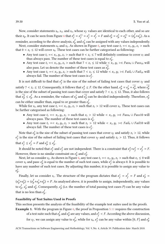
39:30 S. Yoo et al.

Now, consider statements s6, s11 and s3, whose ef values are identical to each other, and so are

their ep . It can be seen from Figure 6 that e6

f = e11

f = e3

f = eff = F and e6

p = e3

p = e11

p = (efp+e

7

p ). As a

reminder, according to the above analysis, efp and e7

p can be assigned with any values independently.

Next, consider statements s4 and s5. As shown in Figure 6, any test case ti =< xi ,yi , zi > such

that 0 < zi ≤ 12 will cover s4. These test cases can be further categorised as following:

• Any test case ti =< xi ,yi , zi > such that 0 < zi ≤ 7 will definitely continue to cover s7 and

thus always pass. The number of these test cases is equal to e7

p .

• Any test case ti =< xi ,yi , zi > such that 7 < zi ≤ 12 while < xi ,yi >∈ Pass9 ∪ Pass10 will

also pass. Let us denote the number of these test cases as e4

p .

• Any test case ti =< xi ,yi , zi > such that 7 < zi ≤ 12 while < xi ,yi >∈ Fail9 ∪ Fail10 will

always fail. The number of these test cases is e4

f .

It is not difficult to find that e4

f is the size of the subset of failing test cases that cover sf and

satisfy 7 < zi ≤ 12. Consequently, it follows that e4

f ≤ F . On the other hand, e4

p = e7

p + e4

p , where e4

p

is the size of the subset of passing test cases that cover and satisfy 7 < zi ≤ 12. Thus, it also follows

that e4

p ≤ efp . As a reminder, the values of e7

p and e4

p can be decided independently. Therefore, e4

p

can be either smaller than, equal to or greater than efp .

While for s5, any test case ti =< xi ,yi , zi > such that zi > 12 will cover s5. These test cases can

be further categorised as following:

• Any test case ti =< xi ,yi , zi > such that zi > 12 while < xi ,yi >∈ Pass9 ∪ Pass10 will

always pass. The number of these test cases is e5

p .

• Any test case ti =< xi ,yi , zi > such that zi > 12 while < xi ,yi >∈ Fail9 ∪ Fail10 will

always fail. The number of these test cases is e5

f .

Note that e5

p is the size of the subset of passing test cases that cover sf and satisfy zi > 12, while

e5

f is the size of the subset of failing test cases that cover sf and satisfy zi > 12. Thus, it follows

that e5

f ≤ eff = F and e5

p ≤ efp .

It should be noted that e4

f and e5

f are not independent. There is a constraint that e4

f +e5

f = eff = F .

However, there is no similar constraint on e4

p and e5

p .

Next, let us consider s2. As shown in Figure 6, any test case ti =< xi ,yi , zi > such that zi ≤ 0 will

cover s2 and pass: e2

p is equal to the number of such test cases, while e2

f is always 0. It is possible to

have any number of such test cases. By adjusting this number, it is possible to assign any value to

e2

p .

Finally, let us consider s1. The structure of the program dictates that e1

f = eff = F and e1

p =

(e3

p+e2

p ) = (efp+e

7

p+e2

p ) = P . As analysed above, it is possible to assign, independently, any values

to efp , e

7

p and e2

p . Consequently, e1

p (i.e. the number of total passing test cases P ) can be any value

that is no less than efp .

Feasibility of Test Suites Used in ProofsThis section presents the analysis of the feasibility of the example test suites used in the proofs.

Example 1. With the program in Figure 6, the proof in Proposition 5.11 requires the construction

of a test suite such that efp and e4

p are any values, and e4

f < F . According the above discussion,

for sf , we can assign any value to efp ; while for s4, e

4

f can be any value within [0, F ] and e4

p



can be either smaller than, equal to or greater than efp . Therefore, it is always possible to

construct such a test suite.

Example 2. With the program in Figure 6, the proof for GP2 in Corollary 5.13 requires the

construction of a test suite such that F = 2, P = 9, s8 (sf ) has eff = 2 = F and e

fp = 5 < P ,

and s9 has e9

f = 1 < F and e9

p = 4 < efp . According to the above analysis, we can assign any

value to efp and any value to P that is no less than e

fp . And for s9, we can have any value

of e9

f within [0, F ] and any value of e9

p within [0, efp ]. Therefore, it is always possible to

construct such a test suite.


construction of a test suite such that F = 2, P = 30, sf has eff = 2 = F and e

fp = 25 < P ,

and s9 has e9

f = 1 < F and e9

p = 25 = efp . Similar to the analysis in Example 2, it is always

possible to construct such a test suite.


construction of a test suite such that F = 5, P = 50, sf has eff = 5 = F and e

fp = 1 < P , and

s4 has e4

f = 4 < F and efp < e4

p = 49 < P . According to the above analysis, for sf , we can

assign any values to eff (i.e. F ) and e

fp ; while for s4, e

4

f can be any value within [0, F ] and e4

p

can be either smaller than, equal to or greater than efp ; and P can be any value that is no

less than either e4

p or efp . Therefore, it is always possible to construct such a test suite.

Example 5. Let us denote the ep values of any two points on the faulty border E as eLp and eHp ,

where eLp < eHp . For the given program in Figure 6, the proof in Lemma 5.10 requires

construction of two test suites, which are referred to as Test Suite A, Test Suite B and

Test Suite C in the following discussion.

Test Suite A: we have e4

f , e5

f , e9

f and e10

f smaller than F , e1

f = e3

f = e6

f = eff = e11

f = F ,

efp = eLp and e1

p = e3

p = e6

p = e11

p = eHp . According to the above analysis, e4

f , e5

f , e9

f and e10

fcan all be less than F simultaneously. And the ef values for s1, s3, s6, sf and s11 are always

equal to F . Besides, for sf , it is always possible to have any value of efp ; while it is always

possible to have any equal value of ep that is larger than efp for s1, s3, s6 and s11. Therefore,

this test suite is feasible.

Test Suite B: we have both e4

f and e5


f = e3

f = e6

f = eff = e9

f = e11

f = F ,

e9

p = eLp and e1

p = e3

p = e6

p = efp = e11

p = eHp . As discussed above, it is always possible to have

both e4

f and e5

f smaller than F . And it is also possible to assign the same value of ef (i.e. F )

to s1, s3, s6, sf , s9 and s11. Moreover, s1, s3, s6, sf and s11 are possible to have the same epvalue that is higher than s9. As a consequence, this test suite is always feasible.

Test Suite C: we have e9

f and e10


f = e3

f = e4

f = e6

f = eff = e11

f = F ,

e4

p = eLp and e1

p = e3

p = e6

p = efp = e11

p = eHp . As discussed above, it is always possible to have

both e9

f and e10

f smaller than F . And it is also possible to assign the same value of ef (i.e. F )

to s1, s3, s4, s6, sf and s11. Moreover, s1, s3, s6, sf and s11 are possible to have the same epvalue that is higher than s4. As a consequence, this test suite is always feasible.

Received February 2007; revised March 2009; accepted June 2009


human competitiveness of genetic programming in spectrum

Documents