human motion database with a binary tree and node transition graphs
TRANSCRIPT

Robotics: Science and Systems 2009Seattle, WA, USA, June 28 - July 1, 2009
1
Human Motion Database with a Binary Tree and
Node Transition Graphs
Katsu Yamane
Disney Research, Pittsburgh
Yoshifumi Yamaguchi
Dept. of Mechano-Informatics
University of Tokyo
Yoshihiko Nakamura
Dept. of Mechano-Informatics
University of Tokyo
Abstract— Database of human motion has been widely used forrecognizing human motion and synthesizing humanoid motions.In this paper, we propose a data structure for storing andextracting human motion data and demonstrate that the databasecan be applied to the recognition and motion synthesis problemsin robotics. We develop an efficient method for building a binarytree data structure from a set of continuous, multi-dimensionalmotion clips. Each node of the tree represents a statisticaldistribution of a set of human figure states extracted fromthe motion clips. We also identify the valid transitions amongthe nodes and construct node transition graphs. Similar statesin different clips may be grouped into a single node, therebyallowing transitions between different behaviors. Using databasesconstructed from real human motion data, we demonstrate thatthe proposed data structure can be used for human motionrecognition, state estimation and prediction, and robot motionplanning.
I. INTRODUCTION
Using a collection of human motion data has been a popular
approach for both analyzing and synthesizing human figure
motions, especially thanks to recent improvements of motion
capture systems. In the graphics field, motion capture data
have been widely used for producing realistic animations for
films and games. A body of research efforts have been directed
to techniques that allow reuse and editing of existing motion
capture to new characters and/or scenarios. In the robotics
field, there are two major applications of such databases:
building a human behavior model for robots to recognize
human motions, and synthesizing humanoid robot motions.
Databases for robotics applications are required to perform
at least the following two functions: First, they have to be
able to categorize human motion into distinct behaviors and
recognize the behavior of a newly observed motion. This is
commonly achieved by constructing a mathematical model that
bridges the continuous motion space and the discrete behavior
space. The problem is that it is often difficult to come up with
a robust learning algorithm for building the models because
raw human motion data normally contain noise and error. The
efficiency of search also becomes a problem as the database
size increases.
Another function is to synthesize a robot motion that adapts
to current situation, which is computationally demanding
because of the large configuration space of humanoid robots.
Motion database is a promising approach because they can
reduce the search space by providing the knowledge on how
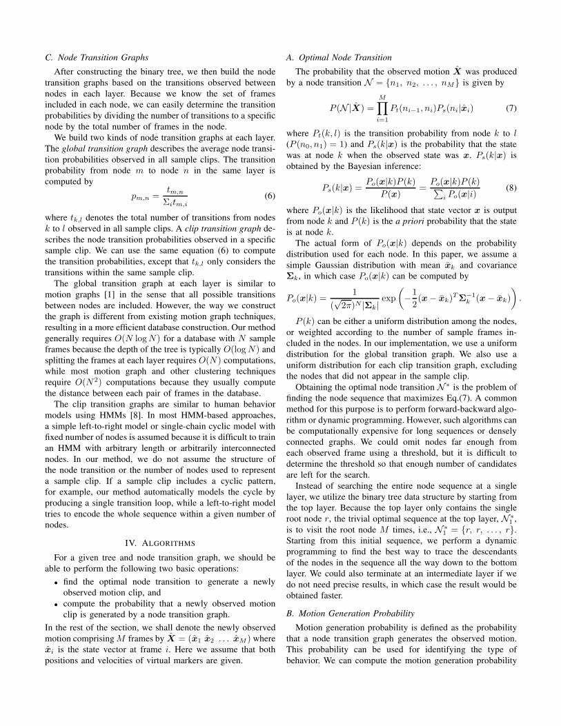
Fig. 1. A binary tree with human motion data. Each x mark representsa frame in one of the sample motion clips. The frames are iteratively splitinto two descendant nodes. Each frame therefore appears once in each layer.Database size can be reduced by making leaf nodes from multiple frames andkeep only the statistical information of the frames included in each node.
human-like robots should move. For this purpose, however,
motion capture data must be organized so that the planner can
effectively extract candidates of motions and/or configurations.
A database should also be able to generate high-quality motion
data, which is also difficult because sample motion data are
usually compressed to reduce the data size.
In this paper, we propose a highly hierarchical data structure
for human motion database. We employ the binary-tree struc-
ture as shown in Fig. 1, which is a classical database structure
widely used in various computer science applications because
of search efficiency. However, constructing a binary-tree struc-
ture from human motion data is not a trivial problem because
there is no straightforward way to split the multi-dimensional,
continuous motion data into two descendant nodes. Our first
contribution is a simple, efficient clustering algorithm for
splitting a set of sample frames into two descendant nodes
to construct a binary tree from human motion data.
We also develop algorithms for basic statistical computa-
tions based on the binary tree structure. Using these algo-

rithms, we can recognize a newly observed motion sequence,
estimate the current state and predict future motions, and plan
new sequences that satisfy given constraints.
Another minor but practically important aspect of the pro-
posed database is the ability to incorporate motion data from
different sources. For example, we may want to include motion
data captured with different marker sets, or include animation
data from a 3D CG film. It is therefore important to choose
a good motion representation to allow different marker sets
and/or kinematic models. In this paper, we propose a scheme
called virtual marker set so that motion data from different
sources can be represented in a uniform way and stored in a
single database.
The rest of this paper is organized as follows. In Section II,
we review related work in graphics and robotics. We then
present the proposed data structure and associated algorithms
in Sections III and IV respectively, and provide several appli-
cation examples in Section V. Section VI demonstrates exper-
imental results using human motion capture data, followed by
concluding remarks.
II. RELATED WORK
In the graphic field, researchers have been investigating how
to reuse and edit motion capture data for new scenes and new
characters. One of the popular approaches is motion graphs,
where relatively large human motion data set is analyzed
to build a graph of possible transitions between postures.
Using the graph, it is possible to synthesize new motion
sequences based on simple user inputs by employing a graph
search algorithm. Kovar et al. [1] proposed the concept of
Motion Graphs where similar postures in a database are au-
tomatically detected and connected to synthesize new motion
sequences. They presented an application of synthesizing new
locomotion sequence that follows a user-specified path. Lee et
al. [2] employed a two-layered statistical model to represent
a database, where the higher-level (coarse) layer is used
for interacting with user inputs and the lower-level (detail)
layer is used for synthesizing whole-body motions. Arikan
et al. [3] also proposed a planning algorithm based on a
concept similar to motion graphs. Related work in the graphics
field mostly focuses on synthesizing new motions from simple
user inputs using, for example, interpolation and numerical
optimization [4].
In robotics, learning from human demonstration, or im-
itation, has been a long-term research issue [5]–[7] and a
number of algorithms have been developed for storing human
motion data and extracting appropriate behaviors. Because
human motion varies at every instance even if the subject
attempts to perform the same motion, it is necessary to
model human behaviors by either statistical models [7], [8],
nonlinear dynamical systems [9], [10], or a set of high-level
primitives [11]. Related work relevant to this paper includes
the Hidden Markov Model (HMM) representation of human
behaviors [8] and the hierarchical motion database based
on HMM [12]. Another hierarchical motion categorization
method is also proposed using neural network models [10].
Fig. 2. Constructing the database.
However, most work in the robotics field is still focused
on robust learning of human behaviors. Scalability of the
motion database or synthesizing transitions between different
behaviors have not been investigated well.
In the vision community, human motion database has been
used to construct human motion models for human tracking
in videos. Sidenbladh et al. [13] proposed a binary-tree data
structure for building a probabilistic human motion model.
They first performed PCA on the entire motion sequence
and then projected each frame data to the principal axes to
construct a binary tree.
III. BUILDING THE DATABASE
The process for building the proposed database is sum-
marized in Fig. 2. The user provides one or more sample
motion clips represented as a pair of root motion and joint
angle sequences, typically obtained by motion capture or hand
animation. The joint angle data are then converted to virtual
marker data through forward kinematics (FK) computation to
obtain the marker positions and velocities, coordinate trans-
formation to remove the trunk motion in the horizontal plane,
and scaling to normalize the subject size. The positions and
velocities of the virtual markers are used to represent the state
of the human figure in each sample frame.
To construct a binary tree, we first create the root node
that contains all frames in the sample motion clips. We then
iteratively split the frames into two descendant nodes using the
method described in Section III-B. After the tree is obtained,
we count the number of transitions among the nodes in each
layer to construct the node transition graphs as described in
Section III-C. The binary tree and node transition graphs are
the main elements of the proposed motion database.
A. Motion Representation
There are several choices for representing the state of a
frame in sample motion clips. A reasonable choice would be
to use joint angles [2], [8] because they uniquely define a
configuration by minimum number of parameters. However,
joint angle representation strictly depends on the skeleton

model and it is difficult to map the states between different
models. In addition, joint angle representation may not be
consistent with visual appearance of the human figure because
the contribution of each joint angle to the Cartesian positions
of the links can vary.
Another possibility is to use point clouds [1]. This method
is independent of underlying skeleton models and also more
intuitive because it directly represent the overall shape of the
figure. The problem is that it is difficult compute the distance
between two poses because registration between two point
clouds is required.
In our implementation, we use a much simpler approach
called virtual marker set, where all motions are represented
by the trajectory (position and velocity) of Nv virtual markers.
The virtual marker set is defined by the database designer so
that it well represents the motions contained in the database,
and can be different from any physical marker sets. The virtual
marker set approach would become similar to the point cloud
method as the number of virtual markers increases, although
each marker in the virtual marker set should be labeled.
If a motion is represented by joint angle trajectories of
a skeleton model, it can be easily converted to the virtual
marker set representation by giving the relationship between
each marker in the virtual marker set and the skeleton used
to represent the original motions. The relationship between
a virtual marker and a skeleton is defined by specifying the
link to which the marker is attached, and giving the relative
position in its local frame. Although this approach requires
some work on the user’s side, it allows the use of multiple
skeleton models with simple distance computation.
After converting the motion data to the virtual marker
set representation, we perform a coordinate transformation to
remove the horizontal movement in the motion and scaling to
normalize the subject size. Each marker position is represented
in a new reference coordinate whose origin is located on the
floor below the root joint, z axis is vertical, and x axis is the
projection of the front direction of the subject model onto the
floor. The marker velocities are also converted to the reference
coordinate.
Formally, a sample motion data matrix X with NS frames
is defined by
X = (x1 x2 . . . xNS) (1)
where xi is the state vector of the i-th sample frame defined
by
xi =(
pTi1 vT
i1 pTi2 vT
i2 . . . pTiNv
vTiNv
)T(2)
and pil and vil are the position and velocity of marker l in
sample frame i. If multiple motion clips are to be stored in a
database, we simply concatenate all state vectors horizontally
and form a single sample motion data matrix.
B. Constructing a Binary Tree
A problem of constructing a binary tree for motion data
is how to cluster the sample frames into groups with similar
states. Most clustering algorithms require a large amount of
computation because they check the distances between all
pairs of frames. This process can take extremely long time
as the database size increases.
Here we propose an efficient clustering algorithm based
on principal component analysis (PCA) and minimum-error
thresholding technique. The motivation for using PCA is that
it determines the axes that best characterize the sample data.
In particular, projecting all samples onto the first principal
axis gives a one-dimensional data set with the maximum
variance, which can then be used for separating distinct
samples using adaptive thresholding techniques developed for
binarizing images.
The process to split node k into two descendant nodes is as
follows. Assume that node k contains nk frames whose mean
state vector is xk. Also denote the sample motion data matrix
of node k by Xk. We compute the zero-mean singular value
decomposition of Xk as
X′Tk = UΣV T (3)
where each column of X ′
k is obtained by subtracting xk from
the original state vectors, Σ is a diagonal matrix whose ele-
ments are the singular values of Xk sorted in the descending
order, and U and V are orthogonal matrices. The columns
of V represents the principal axes of Xk. We obtain the
one-dimensional data set sk by projecting X ′
k onto the first
principal axis by
sk = X′Tk v1 (4)
where v1 denotes the first column of V .
Once the one-dimensional data is obtained, the cluster-
ing problem is equivalent to determining the threshold that
minimizes classification error. We shall use a minimum-error
thresholding technique [14] to determine the optimal threshold.
After sorting the elements of sk and obtaining the sorted vector
s′
k, this method determines the index m such that the data
should be divided between samples m and m + 1 using the
following equation:
m = argmaxi
{
i logσ1
i+ (nk − i) log
σ2
nk − i
}
(5)
where σ1 and σ2 denote the variance of the first i and last
nk − i elements of s′
k, respectively.
We obtain a binary tree by repeating this process until
the division creates a node containing fewer frames than a
predefined threshold. To ensure the statistical meaning of each
node, we also avoid nodes with small number of sample frames
by setting a threshold for minimum frame number. If Eq.(5)
results in a node with fewer number of frames than the latter
threshold, we do not perform the division. Therefore, a node
may not be divided if it contains many similar frames.
Some branches may be shorter than others because we
extend each branch as much as possible and some of them
may hit the thresholds earlier. In such cases, we simply extend
shorter branches by attaching a copy of the leaf node so
that the length of all branches become the same. Each node
therefore can have 0 (leaf nodes), 1 or 2 descendant nodes.
C. Node Transition Graphs
After constructing the binary tree, we then build the node
transition graphs based on the transitions observed between
nodes in each layer. Because we know the set of frames
included in each node, we can easily determine the transition
probabilities by dividing the number of transitions to a specific
node by the total number of frames in the node.
We build two kinds of node transition graphs at each layer.
The global transition graph describes the average node transi-
tion probabilities observed in all sample clips. The transition
probability from node m to node n in the same layer is
computed by
pm,n =tm,n
Σitm,i
(6)
where tk,l denotes the total number of transitions from nodes
k to l observed in all sample clips. A clip transition graph de-
scribes the node transition probabilities observed in a specific
sample clip. We can use the same equation (6) to compute
the transition probabilities, except that tk,l only considers the
transitions within the same sample clip.
The global transition graph at each layer is similar to
motion graphs [1] in the sense that all possible transitions
between nodes are included. However, the way we construct
the graph is different from existing motion graph techniques,
resulting in a more efficient database construction. Our method
generally requires O(N log N) for a database with N sample
frames because the depth of the tree is typically O(log N) and
splitting the frames at each layer requires O(N) computations,
while most motion graph and other clustering techniques
require O(N2) computations because they usually compute
the distance between each pair of frames in the database.
The clip transition graphs are similar to human behavior
models using HMMs [8]. In most HMM-based approaches,
a simple left-to-right model or single-chain cyclic model with
fixed number of nodes is assumed because it is difficult to train
an HMM with arbitrary length or arbitrarily interconnected
nodes. In our method, we do not assume the structure of
the node transition or the number of nodes used to represent
a sample clip. If a sample clip includes a cyclic pattern,
for example, our method automatically models the cycle by
producing a single transition loop, while a left-to-right model
tries to encode the whole sequence within a given number of
nodes.
IV. ALGORITHMS
For a given tree and node transition graph, we should be
able to perform the following two basic operations:
• find the optimal node transition to generate a newly
observed motion clip, and
• compute the probability that a newly observed motion
clip is generated by a node transition graph.
In the rest of the section, we shall denote the newly observed
motion comprising M frames by X = (x1 x2 . . . xM ) where
xi is the state vector at frame i. Here we assume that both
positions and velocities of virtual markers are given.
A. Optimal Node Transition
The probability that the observed motion X was produced
by a node transition N = {n1, n2, . . . , nM} is given by
P (N|X) =M∏
i=1
Pt(ni−1, ni)Ps(ni|xi) (7)
where Pt(k, l) is the transition probability from node k to l
(P (n0, n1) = 1) and Ps(k|x) is the probability that the state
was at node k when the observed state was x. Ps(k|x) is
obtained by the Bayesian inference:
Ps(k|x) =Po(x|k)P (k)
P (x)=
Po(x|k)P (k)∑
i Po(x|i)(8)
where Po(x|k) is the likelihood that state vector x is output
from node k and P (k) is the a priori probability that the state
is at node k.
The actual form of Po(x|k) depends on the probability
distribution used for each node. In this paper, we assume a
simple Gaussian distribution with mean xk and covariance
Σk, in which case Po(x|k) can be computed by
Po(x|k) =1
(√
2π)N |Σk|exp
(
−1
2(x − xk)T
Σ−1
k (x − xk)
)
.
P (k) can be either a uniform distribution among the nodes,
or weighted according to the number of sample frames in-
cluded in the nodes. In our implementation, we use a uniform
distribution for the global transition graph. We also use a
uniform distribution for each clip transition graph, excluding
the nodes that did not appear in the sample clip.
Obtaining the optimal node transition N ∗ is the problem of
finding the node sequence that maximizes Eq.(7). A common
method for this purpose is to perform forward-backward algo-
rithm or dynamic programming. However, such algorithms can
be computationally expensive for long sequences or densely
connected graphs. We could omit nodes far enough from
each observed frame using a threshold, but it is difficult to
determine the threshold so that enough number of candidates
are left for the search.
Instead of searching the entire node sequence at a single
layer, we utilize the binary tree data structure by starting from
the top layer. Because the top layer only contains the single
root node r, the trivial optimal sequence at the top layer, N ∗
1,
is to visit the root node M times, i.e., N ∗
1= {r, r, . . . , r}.
Starting from this initial sequence, we perform a dynamic
programming to find the best way to trace the descendants
of the nodes in the sequence all the way down to the bottom
layer. We could also terminate at an intermediate layer if we
do not need precise results, in which case the result would be
obtained faster.
B. Motion Generation Probability
Motion generation probability is defined as the probability
that a node transition graph generates the observed motion.
This probability can be used for identifying the type of
behavior. We can compute the motion generation probability

by summing up the probability of generating the motion by all
possible node transitions. However, there may be huge number
of possible node transitions for long motions or large transition
graphs.
An alternative used in this paper is to use the dynamic
programming described in the previous subsection to find
multiple node sequences. Because the algorithm returns node
sequences in the descending order of probability, we can
approximate the total motion generation probability by using
the top few node sequences.
V. APPLICATIONS
A. State Estimation and Prediction
Estimating the current state is accomplished by taking the
last node in the most likely node transition in the global node
transition graph. Once the node transition is estimated with
high probability, we can then predict the next action by tracing
the node transition graph. By combining the probability of
the node transition and the probability of the future transition
candidate, we can also obtain the confidence of the prediction.
B. Motion Recognition
Motion recognition is the process to find a motion clip in the
database that best matches a newly observed motion sequence.
This is accomplished by comparing the motion generation
probability from the clip transition graphs.
C. Motion Planning
The global transition graph can also be used for planning a
new motion sequence subject to kinematic constraints. In addi-
tion, because the tree has multiple layers that model the sample
clips at different granularities, motion planning can also be
performed at different precision levels. The only issue is how
to compute the motion of the root in the horizontal plane
because those information are removed from the database.
Our solution is to use the marker velocity data to obtain
the root velocity, and then integrate the velocity to obtain
root trajectory. The velocity can be obtained by employing
a numerical inverse kinematics algorithm, which essentially
solves the following linear equation:
θ = Jv (9)
where θ is the joint velocities including the root linear and
angular velocities, v is the vector of all marker velocities
extracted from the mean vector of a node, and J is the
Jacobian matrix of the marker positions with respect to joint
angles. This is usually an overconstrained IK problem because
the virtual marker set contains more markers than necessary to
determine the joint motion. We therefore apply the singularity-
robust (SR) inverse [15] of J to obtain θ.
VI. RESULTS
A. Sample Data Set
We use two different sets of data to demonstrate the
generality of our approach. The minimum number of sample
TABLE I
PROPERTIES OF THE TWO DATABASES.
Database 1 Database 2
# of frames 5539 11456# of layers 17 16# of nodes 1372 1527
# of nodes in bottom layer 167 205
frames in a node is set to 16 in both databases. The properties
of the databases are summarized in Table I.
The first set (Database 1) consists of 19 motion clips
including a variety of jog, kick, jump, and walk motions, all
captured separately in the motion capture studio at University
of Tokyo. The motions were captured using our original
marker set consisting of 34 markers. This marker set is also
used as the virtual marker set to construct all the databases
in the experiments. Database 1 is used to demonstrate the
analysis experiments.
The second set (Database 2) is generated from selected clips
in a publicly available motion library [16] and will be used
for the planning experiment. The database includes two long
locomotion sequences with forward, backward and sideward
walk of the same subject. Although Database 2 contains twice
as many sample frames as Database 1, it resulted in relatively
small number of layers and nodes probably because they
consist of similar motions and hit the minimum frame number
threshold earlier.
Because the virtual marker set consists of 34 markers, the
dimension of the state vector is 204.
B. Properties of the Database
We first visualize Database 1 to investigate its properties.
In Fig. 3, the spheres (light-blue for readers with color figures)
represent all nodes in the bottom layer and the red lines
represent the transitions among the nodes. The white mesh
represents the plane of first and second principal axes. The
projection onto the first-second principal axes plane is also
shown in Fig. 4. Figure 5 shows the nodes and global transition
graphs at layers 4 and 7, with the top layer numbered layer 1.
The location of each node is computed by projecting its
mean vector onto the first three principal components of the
root node of the tree. The size of the node is proportional to
the maximum singular value of the sample motion data matrix
of the node.
Figure 6 shows the mean marker positions and velocities
of the nodes marked in Fig. 4. These images clearly show the
geometrical meaning of the first and second principal axis: the
first axis represents the vertical velocity and the second axis
represents which leg is raised. Apparently there is no verbally
explainable meaning in the third axis.
Figure 7 shows the node transition graphs of two represen-
tative clips. As expected from the above observation, motions
such as jump that involves mostly the vertical motion stay in
the first and third axes plane, while jog, kick and walk motions
stay in the second and third axes plane.

Fig. 3. Visualization of the database in the three principal axes space.
Fig. 4. Visualization of the database in the first (horizontal) and second(vertical) principal axes space.
C. State Estimation and Prediction
We experimented the state estimation ability by providing
the first 0.2 s of a novel kick motion by the same subject and
a jump motion by a different subject. The results are shown
in Figures 8 and 9 respectively. Note that the global node
transition is used to compute the best node sequence, although
only the node transition in relevant sample clip is drawn in
each figure for clarity.
In both cases, the database could predict the subjects’
actions before they actually occurred. In Fig. 8, all nodes
on the identified node sequence (drawn as yellow spheres)
Fig. 5. Nodes and global transition graphs at layers 4 and 7.
Fig. 6. Mean marker positions and velocities of selected nodes. The linesrooted at markers denote the velocities. From left to right: nodes 1369, 1362,1361, and 1366 as marked in Fig. 4.
Fig. 7. Node transition graphs of selected clips. Left: jump, right: kick.
are included in the transition graph of the kick samples. The
last node in the sequence is likely to transit to the dark blue
node in the left figure with the probability of 0.36, which
corresponds to the marker positions and velocities in the right
figure. Similarly, the result of Fig. 9 indicates that the database
can correctly identify that the subject is in preparation for a
jump.
D. Motion Recognition
Figures 10–11 show the results of motion recognition exper-
iments. The three graphs in Fig. 10 show differences between
layers for the same observation. We computed the motion
generation probability of new motions with respect to the
node transition graph of each sample motion clip. Because the
new motion is 2.5 s long and computation of the probabilities
takes long time, we computed the probability of generating the
Fig. 8. Result of state estimation and prediction for a kick motion of thesame subject. Left: the nodes on the identified node transition are drawn inyellow. Right: the marker positions and velocities corresponding to the bluenode in the left figure.

Fig. 9. Result of state estimation and prediction for a jump motion of adifferent subject. Left: the nodes on the identified node transition are drawnin yellow. Right: the marker positions and velocities corresponding to the bluenode in the left figure.
Fig. 11. Time profile of generation probability of a walk motion of a differentsubject (bottom layer).
sequences within a sliding window of width 0.4 s. The graphs
depict the time evolution of probabilities when we moved the
window from [0.0s, 0.4s] to [2.0s, 2.4s]. The lines are colored
according to the type of motions. We use same line color and
type for very similar sample clips for clarity of presentation.
The first three graphs show the probability of a new walk
motion by the same subject as the database, while a walk
motion from a different subject was used for Fig. 11. These
results show that the model can successfully recognize the
type of observed motion even for different subjects. It is also
suggested that the statistical models at different layers have
different granularity levels because the variation of probabili-
ties is smaller for upper layers. In particular, similar motions
such as walk and jog begin to merge at layer 7.
Figure 12 show the result at the bottom layer for a com-
pletely unknown motion (lifting an object from the floor). It is
clear that the database cannot tell whether the motion is jump
or kick, which is intuitively reasonable because these three
motions start from small bending.
Fig. 12. Time profile of generation probability of a lifting motion (bottomlayer).
Fig. 13. Result of motion planning. Left: path of the root in horizontal plane.Right: postures at selected frames.
E. Motion Planning
We performed a simple motion planning test with only start
and goal position constraints. Figure 13 shows the planned
motion when the goal position is given as 2.0 m front and
1.0 m left of the current position. The planner outputs a
reasonable motion under the available samples, which is to
walk forward for 2 m and do a side walk to the left for 1 m. We
can observe that the feet occasionally penetrate the floor. We
would need the contact status information to fix this problem.
VII. CONCLUSION
In this paper, we proposed a new data structure for stor-
ing multi-dimensional, continuous human motion data, and
demonstrated its basic functions through experiments. The
main contributions of the paper are summarized as follows:
1) We proposed a method for constructing a binary tree data
structure from human motion data. We applied PCA and
a minimum-error thresholding technique to efficiently
find the optimal clustering of sample frames.
2) We proposed to build a global node transition graph
representing the node transitions in all sample clips,
as well as a clip transition graph representing the node
transitions in each sample motion clip.
3) We developed two algorithms for computing the most
probable node transition and generation probability for

Fig. 10. Time profile of generation probability of a new walk motion of the same subject. From left to right: bottom layer, layer 10, layer 7.
a given new motion sequence, based on the binary tree
data structure.
4) We demonstrated three applications of the proposed
database through experiments using real human motion
data.
There are several functions yet to be addressed by our
database. We currently do not support incremental learning
of new motions because all sample frames must be available
to perform the PCA. If the new sample clips do not dras-
tically change the distribution of whole samples, we could
apply one of the extensions of PCA for online learning tech-
niques [17]. Some techniques for balancing binary trees for
multi-dimensional data could also be employed to reorganize
the tree [18].
It should be relatively easy to add segmentation and cluster-
ing functions because the sample motion clips are abstracted
by node transition graphs. We can easily detect same or similar
node transitions in different motion clips, which could be used
for segmentation. Clustering of sample clips can be achieved
by evaluating the distance between motion clips based on
their node transition graphs and applying standard clustering
algorithms [19].
Our current database only contains the marker position and
velocity data. It would be interesting to add other modalities
such as contact status, contact forces, and muscle tensions. In
particular, we would be able to solve the contact problem in
our planning experiment if we have access to the contact status
information. Contact force and muscle tension information
would also help generating physically feasible motions for
humanoid robots.
ACKNOWLEDGEMENTS
Part of this work was conducted while the first author was
at University of Tokyo. The authors gratefully acknowledge
the support by the Ministry of Education, Culture, Sports,
Science and Technology, Japan through the Special Coordi-
nation Funds for Promoting Science and Technology, “IRT
Foundation to Support Man and Aging Society.”
REFERENCES
[1] L. Kovar, M. Gleicher, and F. Pighin, “Motion graphs,” ACM Transac-
tions on Graphics, vol. 21, no. 3, pp. 473–482, 2002.
[2] J. Lee, J. Chai, P. S. A. Reitsma, J. K. Hodgins, and N. S. Pollard,“Interactive Control of Avatars Animated With Human Motion Data,”ACM Transactions on Graphics, vol. 21, no. 3, pp. 491–500, July 2002.
[3] O. Arikan and D. A. Forsyth, “Synthesizing Constrained Motions fromExamples,” ACM Transactions on Graphics, vol. 21, no. 3, pp. 483–490,July 2002.
[4] A. Safonova and J. Hodgins, “Interpolated motion graphs with optimalsearch,” ACM Transactions on Graphics, vol. 26, no. 3, p. 106, 2007.
[5] C. Breazeal and B. Scassellati, “Robots that imitate humans,” Trends in
Cognitive Science, vol. 6, no. 11, pp. 481–487, 2002.[6] S. Schaal, A. Ijspeert, and A. Billard, “Computational approaches to
motor learning by imitation,” Phylosophical Transactions of the Royal
Society of London B: Biological Sciences, vol. 358, pp. 537–547, 2003.[7] A. Billard, S. Calinon, and F. Guenter, “Discriminative and adaptive
imitation in uni-manual and bi-manual tasks,” Robotics and Autonomous
Systems, vol. 54, pp. 370–384, 2006.[8] T. Inamura, I. Toshima, H. Tanie, and Y. Nakamura, “Embodied symbol
emergence based on mimesis theory,” International Journal of Robotics
Research, vol. 24, no. 4/5, pp. 363–378, 2004.[9] A. Ijspeert, J. Nakanishi, and S. Schaal, “Movement imitation with
nonlinear dynamical systems in humanoid robots,” in Proceedings of
International Conference on Robotics and Automtation, 2002, pp. 1398–1403.
[10] H. Kadone and Y. Nakamura, “Symbolic memory for humanoid robotsusing hierarchical bifurcations of attractors in nonmonotonic neuralnetworks,” in Proceedings of International Conference on Intelligent
Robots and Systems, 2005, pp. 2900–2905.[11] D. Bentivegna, C. Atkeson, and G. Cheng, “Learning tasks from
observation and practice,” Robotics and Autonomous Systems, vol. 47,no. 2–3, pp. 163–169, 2004.
[12] D. Kulic, W. Takano, and Y. Nakamura, “Incremental learning, clusteringand hierarchy formation of whole body motion patterns using adaptivehidden markov chains,” International Journal of Robotics Research,vol. 27, no. 7, pp. 761–784, 2008.
[13] H. Sidenbladh, M. Black, and L. Sigal, “Implicit probabilistic modelsof human motion for synthesis and tracking,” in European Conference
on Computer Vision, 2002, pp. 784–800.[14] J. Kittler and J. Illingworth, “Minimum error thresholding,” Pattern
Recognition, vol. 19, no. 1, pp. 41–47, 1986.[15] Y. Nakamura and H. Hanafusa, “Inverse Kinematics Solutions with
Singularity Robustness for Robot Manipulator Control,” Journal of
Dynamic Systems, Measurement, and Control, vol. 108, pp. 163–171,1986.
[16] “CMU graphics lab motion capture database,” http://mocap.cs.cmu.edu/.[17] M. Artac, M. Jogan, and A. Leonardis, “Incremental pca or on-line visual
learning and recognition,” in Proceedings of the 16 th International
Conference on Pattern Recognition, 2002, pp. 30 781–30 784.[18] V. K. Vaishnavi, “Multidimensional balanced binary trees,” IEEE Trans-
actions on Computers, vol. 38, no. 7, pp. 968–985, 1989.[19] J. Ward, “Hierarchical grouping to optimize an objective function,”
Journal of the American Statistical Association, vol. 58, pp. 236–244,1963.