hybrid neural networks for learning the trend in time serieshybrid neural networks for learning the...

Hybrid Neural Networks for Learning the Trend in Time Series

Tao Lin∗, Tian Guo∗, Karl AbererSchool of Computer and Communication Sciences

Ecole polytechnique federale de LausanneLausanne, Switzerland

{tao.lin, tian.guo, karl.aberer}@epfl.ch

AbstractTrend of time series characterizes the intermediateupward and downward behaviour of time series.Learning and forecasting the trend in time seriesdata play an important role in many real applica-tions, ranging from resource allocation in data cen-ters, load schedule in smart grid, and so on. In-spired by the recent successes of neural networks,in this paper we propose TreNet, a novel end-to-end hybrid neural network to learn local and globalcontextual features for predicting the trend of timeseries. TreNet leverages convolutional neural net-works (CNNs) to extract salient features from localraw data of time series. Meanwhile, consideringthe long-range dependency existing in the sequenceof historical trends, TreNet uses a long-short termmemory recurrent neural network (LSTM) to cap-ture such dependency. Then, a feature fusion layeris to learn joint representation for predicting thetrend. TreNet demonstrates its effectiveness by out-performing CNN, LSTM, the cascade of CNN andLSTM, Hidden Markov Model based method andvarious kernel based baselines on real datasets.

1 IntroductionTime series, which is a sequence of data points in time order,is being generated in a wide spectrum of domains, such asmedical and biological experimental observations, daily fluc-tuation of stock markets, power consumption records, perfor-mance monitoring of data centres, and so on. In many ap-plications, users are interested in understanding the evolvingtrend in time series and forecasting the trend, since the con-ventional prediction on specific data points could deliver verylittle information about the semantics and dynamics of the un-derlying process generating the time series. For instance, timeseries in Figure 1 are from the power consumption dataset1. Figure 1(a) shows some raw data points of time series.Though point A and B have approximately the same value,the underlying system is likely to be in two different states

∗These two authors contributed equally.1https://archive.ics.uci.edu/ml/datasets/Individual+household

+electric+power+consumption

when it outputs A and B, because A is in an upward trendwhile B is in a downward trend [Wang et al., 2011]. Onthe other hand, even when two points with the similar valueare both in the upward trend, e.g, point A and C, the differ-ent slopes and durations of the trends where point A and Clocate, could also indicate different states of the underlyingprocess.

Particularly, in this paper we are interested in the trend oftime series which measures the intermediate behaviour, i.e.upward or downward pattern of time series. It is charac-terized by the slope and duration [Wang et al., 2011]. Forinstance, Figure 1(b) and (c) show one time series and theassociated trend evolution over the time series. Given suchinformation, we aim to predict the duration and slope of thesubsequent trend. Learning and forecasting trends are quiteuseful in a wide range of applications. For instance, in thesmart energy domain, knowing the predictive trend of powerconsumption time series enables energy providers to sched-ule power supply and maximize energy utilization [Zhao andMagoules, 2012]. in the stock market, due to its high volatil-ity and noisy environment. In reality predicting stock pricetrends is preferred over the prediction of the stock market ab-solute values [Atsalakis and Valavanis, 2009]. Predicting thetrend of stock price time series provides the insight into theintermediate behaviours of economic actors [Atsalakis andValavanis, 2009].

Meanwhile, in recent years neural networks have shownthe dramatical power in a wide spectrum of domains, e.g.,natural language processing, computer vision, speech recog-nition, time series analysis, etc [Wang et al., 2016b; Sutskeveret al., 2014; Yang et al., 2015; Lipton et al., 2015; Guoet al., 2016]. For time series data, two mainstream ar-chitectures, convolutional neural network (CNN) and recur-rent neural network (RNN), have been exploited in differ-ent tasks, e.g., RNN in time series classification [Lipton etal., 2015] and CNN in activity recognition and snippet learn-ing [Liu et al., 2015; Yang et al., 2015]. RNN is power-ful in discovering the dependency in sequence data [Chunget al., 2014] and particularly the Long Short-Term Memory(LSTM) RNN works well on sequence data with long-termdependencies [Chung et al., 2014; Hochreiter and Schmid-huber, 1997] due to the internal memory mechanism. CNNexcels in extracting effective representation of local saliencefrom raw data of time series by enforcing a local connectivity

Proceedings of the Twenty-Sixth International Joint Conference on Artificial Intelligence (IJCAI-17)

2273

Figure 1: (a) Underlying information in time series. (b) Time series. (c) Sequence of trends associated with the time series.

between neurons [Yang et al., 2015; Hammerla et al., 2016;Wang and Oates, 2015].

In this paper, we focus on learning and forecasting thetrends in time series via neural networks. This involves learn-ing different aspects of the data. On the one hand, the trendvariation of time series is a sequence of historical trends car-rying the long-term contextual information of time series andnaturally affects the evolution of the following trend. On theother hand, the recent raw data points of time series [Wang etal., 2011], which represent the local behaviour of time series,affects the evolving of the following trend as well and haveparticular predictive power for abruptly changing trends. Forinstance, in Figure 2(b), trend 1, 2 and 3 present a continu-ous upward pattern corresponding to the time series beforethe prediction time instant. Then when we aim at predictingthe subsequent trend of time series, the previous three succes-sive upward trends outline a probable increasing trend after-wards. However, the local data points around the end of thethird trend as is shown in Figure 2(a), e.g., data points in thered circle, indicate that time series could stabilize and evendecrease. The true data after the third trend indeed presenta decreasing trend indicated by the blue dotted segment. Inthis case, the subsequent trend has more dependency on thelocal data points. Therefore, it is highly desired to developa systematic way to model such hidden and complementarydependencies in time series.

Figure 2: (a) Trend prediction on time series. (b) Associated se-quence of trends.

To this end, we propose an end-to-end hybrid neural net-work, referred to as TreNet. In particular, it consists of anLSTM recurrent neural network to capture the long depen-dency in historical trends, a convolutional neural network toextract local features from local raw data of time series, anda feature fusion layer to learn joint representation to take ad-vantage of both features drawn from CNN and LSTM. Such

joint representation is used for the trend forecasting. The ex-perimental analysis on real datasets demonstrates that TreNetoutperforms CNN, RNN, the cascade of CNN and RNN, anda variety of baselines in term of trend prediction accuracy.

The rest of the paper is organized as follows. Section 2presents related work. In Section 3, we present the proposedTreNet. Section 4 reports experimental results and the paperis concluded in Section 5.

2 Related WorkTraditional learning approaches over trends of time seriesmainly make use of Hidden Markov Models (HMMs) [Wanget al., 2011; Matsubara et al., 2014]. HMMs maintain short-term state dependences, i.e., the memoryless Markov prop-erty and predefined number of states, which requires signifi-cant task-specific knowledge. RNNs can capture long-termdependencies in sequence data. Previous time series seg-mentation approaches [Wang et al., 2011; Yuan, 2015] focuson achieving a meaningful segmentation, rather than mod-eling the relation in segments and therefore are not suitablefor forecasting trends. Multi-step ahead prediction is anotherway to realize trend prediction by fitting the predicted valuesto estimate the trend [Chang et al., 2012]. However, multi-step ahead prediction of time series is non-trivial [Venka-traman et al., 2015] and suffers from the accumulative pre-diction errors [Taieb and Atiya, 2016; Bao et al., 2014]. Inthis paper, we concentrate on directly learning trends throughneural networks.

RNNs have recently shown promising results in a varietyof applications, especially when there exist sequential depen-dencies in data [Chung et al., 2014; Sutskever et al., 2014].Long short-term memory (LSTM) [Hochreiter and Schmid-huber, 1997; Chung et al., 2014], a class of recurrent neuralnetworks with sophisticated recurrent hidden and gated units,are particularly successful and popular due to its ability tolearn hidden long-term sequential dependencies. [Lipton etal., 2015] uses LSTMs to recognize patterns in multivariatetime series, especially for multi-label classification of diag-noses. [Malhotra et al., 2015] evaluate the ability of LSTMsto detect anomalies in ECG time series.

CNNs are often used to learn effective representation oflocal salience from raw data [Vinyals et al., 2015; Donahue etal., 2015]. [Hammerla et al., 2016; Yang et al., 2015] makeuse of CNNs to extract features from raw time series datafor activity/action recognition. [Liu et al., 2015] focuses on


2274

the prediction of periodical time series values by using CNNand embedding time series with neighbors in the temporaldomain. Our proposed TreNet will combine the strengths ofboth LSTM and CNN and form a novel and unified neuralnetwork architecture for trend forecasting.

Hybrid neural networks, which combines the strengths ofvarious neural networks, are receiving increasing interest inthe computer vision domain, such as image captioning [Maoet al., 2014; Vinyals et al., 2015; Donahue et al., 2015], imageclassification [Wang et al., 2016a], action recognition [Ballaset al., 2015; Donahue et al., 2015] and so on. But efficientexploitation of such hybrid architectures has not been wellstudied for time series data, especially the trend forecastingproblem. [Ballas et al., 2015] utilizes CNNs over images in acascade of RNNs in order to capture the temporal features forclassification. [Bashivan et al., 2015] transforms EEG datainto a sequence of topology-preserving multi-spectral imagesand then trains a cascaded convolutional-recurrent networkover such images for EEG classification. [Wang et al., 2016a;Mao et al., 2014] propose the CNN-RNN framework to learna shared representation for image captioning and classifica-tion problems.

3 Hybrid neural networks for Learning theTrend

In this section, we provide the formal definition of the trendlearning and forecasting problem. Then, we present the pro-posed TreNet.

3.1 Problem Formulation

We define time series as a sequence of data points X ={x1, . . . , xT }, where each data point xt is real-valued andsubscript t represents the time instant. The historical trend se-quence ofX is a series of historical trends overX , denoted byT = {〈`k, sk〉}. Each element of T , e.g., 〈`k, sk〉 describesa linear function over a certain subsequence (or segment) ofX and corresponds to a trend in X . `k and sk respectivelyrepresent the duration and slope of trend k. `k is measuredin terms of the time range covered by trend k. Both `k andsk are continuous values. Trends in T are time ordered andnon-overlapping. The durations of all the trends in T address∑k

`k = T .

Meanwhile, as we discussed in Section 1, local raw dataof time series affects the evolving of trend and thus we de-fine the local data w.r.t. each historical trend in T as aset of data points of size w. Formally, it is denoted byL = {〈xtk−w, . . . , xtk〉}, where tk is the ending time of trendk in T . w is empirically selected, which will be discussed inSection 4.

Then, we aim to propose a neural network based approachto learn a function f(T ,L) to predict the subsequent trend〈l, s〉. In this paper, we focus on univariate time series. Thefollowing proposed method can be naturally generalized tomultivariate time series as well by augmenting the trainingdata.

3.2 TreNetIn this part, we first present the overview of the proposed hy-brid architecture TreNet for the trend forecasting. Then wewill detail each component of TreNet.

OverviewThe idea of TreNet is to combine CNN and LSTM to utilizetheir representation abilities on different aspects of data (i.e.,L and T ) and to learn a joint feature used for the trend pre-diction.

Technically, TreNet is designed to learn a predictive func-tion 〈l, s〉 = f(R(T ), C(L)). R(T ) is derived by trainingthe LSTM over the sequence T to capture the dependencyin historical trend evolving, while C(L) corresponds to localfeatures extracted by CNN from sets of local data in L. Thelong-term and local features respectively captured by LSTMand CNN, i.e., R(T ) and C(L) convey complementary infor-mation pertaining to the trend varying. Then, the feature fu-sion layer merges the features for forecasting the subsequenttrend. Finally, the trend prediction is realized by the functionf( , ), which corresponds to the feature fusion and outputlayers as is shown in Figure 3.

Learning the dependency in the historical trend sequenceDuring the training phase the duration `k and slope sk of eachtrend k in sequence T are fed into the LSTM layer of TreNet.Each j-th neuron in the LSTM layer maintains a memory cjkat step k. The output hjk or the activation of this neuron isthen expressed as: hjk = ojktanh(c

jk), where ojk is an output

gate of a LSTM neuron [Hochreiter and Schmidhuber, 1997;Chung et al., 2014]. At each step k, the hidden activation hk

is the output to the feature fusion layer.ojk is calculated by

ojk = σ(Wo[`k sk] +Uohk−1 + Vock)j (1)

where [`k sk] is the concatenation of the duration and slopeof the trend k, hk−1 and ck are the vectorization of the acti-vations of {hjk−1} and {cjk}, and σ is a logistic sigmoid func-tion. Then, the memory cell cjk is updated through partiallyforgetting the existing memory and adding a new memorycontent cjk:

cjk = f jkcjk−1 + ijk c

jk , c

jk = tanh(Wc[`k sk] +Uchk−1)

j

(2)

The extent to which the existing memory is forgotten is mod-ulated by a forget gate f jk , and the degree to which the newmemory content is added to the memory cell is modulated byan input gate ijk. Then, such gates are computed by

f jk = σ(Wf [`k sk] +Ufhk−1 + Vfck−1)j (3)

ijk = σ(Wi[`k sk] +Uihk−1 + Vick−1)j (4)

Vf and Vi are diagonal matrices.

Learning local features from raw data of time seriesWhen the k-th trend in T is fed to LSTM, the correspond-ing local raw time series data points 〈xtk−w, . . . , xtk〉 in L


2275

Figure 3: Illustration of the hybrid architecture of TreNet. (best viewed in colour)

is input to the CNN part of TreNet. CNN consists of Hstacked layers of 1-d convolutional, activation and poolingoperations. Each layer has a specified number of filters of aspecified filter size. Each filter on a layer sweeps through theentire set of data points to exact local features. The output ofCNN in TreNet is the concatenation of max-pooling outputson the last layer H [Donahue et al., 2015].

Feature fusion and output layersThe feature fusion layer combines the output representationsfrom LSTM and CNN, i.e., R(T ) and C(L), to form a jointfeature. Then, such a joint feature is fed to the output layer toprovide the trend prediction. Particularly, we first map R(T )and C(L) to the same feature space and then add them to-gether to obtain the activation of the feature fusion layer [Maoet al., 2014]. The output layer is a fully-connect layer follow-ing the feature fusion layer. Mathematically, the prediction ofTreNet is expressed as:

〈l, s〉 = f(R(T ), C(L))=W o · φ(W r ·R(T ) +W c · C(L))︸︷︷︸

feature fusion

+bo (5)

where φ(·) is element-wise leaky ReLU activation functionand + here denotes the element-wise addition. W o and boare the weights and bias of the output layer.

To train TreNet, we adopt the squared error function plus aregularization term as:

J(W , b ; T ,X ) = 1

|T |

|T |∑k=1

[(lk − lk)2 + (sk − sk)2

]+ λ‖W ‖2

(6)where W and b represent all the weight and bias parametersin TreNet, λ is a hyperparameter for the regularizationterm. The cost function is differentiable and the architectureof TreNet allows the gradient of loss function (6) to bebackpropagated to both LSTM and CNN parts.

4 Experimental AnalysisIn this section, we report experimental results to demonstratethe advantage of TreNet by comparing to a variety of base-lines.

4.1 Experiment SetupDataset:• Power Consumption (PC). This dataset2 contains mea-

surements of electric power consumption with a one-minute sampling rate over a period of almost 4 years. Weuse the voltage time series throughout the experiments.• Gas Sensor (GasSensor). This dataset3 contains the

recordings of chemical sensors exposed to dynamic gasmixtures at varying concentrations. The measurementwas constructed by the continuous acquisition of thesensor array signals for a duration of about 12 hourswithout interruption. We mainly use the gas mixturetime series regarding Ethylene and Methane in air.• Stock Transaction (Stock): This dataset is extracted

from Yahoo Finance and contains the daily stock trans-action information in New York Stock Exchange from1950-10 to 2016-4.

For the ease of result interpretation, the slope of thetrends is represented by the angle in a bounded value range[−90, 90]. The duration of trends is measured by the numberof data points covered by the trend. Data instances are builtby combining historical trend sequence, local raw data andthe target trend w.r.t. each time series subsequence. We thendo random shuffling over such data instances, where 10% ofthe data instances is held out as the testing dataset and therest is used for cross-validation. Totally, there exist 42279instances in the power consumption dataset, 4418 instancesfor the gas sensor dataset and 10014 instances for the stockdataset.Baselines: We compare TreNet with the following six base-lines:• CNN. This baseline method predicts the trend by using

CNN over the raw data of time series to learn featuresused for the trend forecasting.• LSTM. This method uses LSTM to learn the trend se-

quence T and then predicts the trend.2https://archive.ics.uci.edu/ml/datasets/Individual+household

+electric+power+consumption3https://archive.ics.uci.edu/ml/datasets/Gas+sensor+

array+under+dynamic+gas+mixtures


2276

• ConvNet+LSTM(CLSTM). It is based on the cascadestructure of ConvNet and LSTM proposed in [Bashivanet al., 2015] which feeds the features learnt by ConvNetover time series raw data to an LSTM and obtains theprediction from the LSTM.• Support Vector Regression (SVR). A family of support

vector regression based approaches with different ker-nel methods are used for the trend forecasting. We con-sider three commonly used kernels [Liu et al., 2015],i.e., Radial Basis kernel (SVRBF), Polynomial kernel(SVPOLY), Sigmoid kernel (SVSIG). The trend se-quence and the corresponding set of local time seriesdata are concatenated as the input features to such SVRapproaches.• Pattern-based Hidden Markov Model (pHMM).

[Wang et al., 2011] proposed a pattern-based hiddenMarkov model (HMM), which segments the time seriesand models the dependency in segments via HMM. Thederived HMM model is used to predict the state of timeseries and then to estimate the trend based on the state.• Naive. This is the naive approach which takes the dura-

tion and slope of the last trend as the prediction for thenext one.

Evaluation metric: We evaluate the predictive performanceof TreNet and baselines in terms of Root Mean Square Error(RMSE). The lower the RMSE, the more accurate the predic-tions.Training: In TreNet, CNN has two stacked convolutionallayers, which have 32 filters of size 2 and 4. The numberof memory cells in LSTM is 600. In addition to the learningrate, the number of neurons in the feature fusion layer is cho-sen from the range {300, 600, 900, 1200} to achieve the bestperformance.

We use dropout and L2 regularization to control the ca-pacity of neural networks to prevent overfitting, and set thevalues to 0.5 and 5 × 10−4 respectively for all datasets[Mao et al., 2014]. Regarding the SVR based approaches,we carefully tune the parameters c (error penalty), d (de-gree of kernel function), and γ (kernel coefficient) forkernels. Each parameter is selected from the sets c ∈{10−5, 10−4, . . . , 1, . . . , 104, 105}, d ∈ {1, 2, 3}, γ ∈{10−5, 10−4, . . . , 1, . . . , 105} respectively.

4.2 Experiment ResultsTable 1 studies the prediction performances of TreNet andbaselines on different datasets. For the approaches requiringlocal raw data in the training data (i.e., SVRBF, SVPOLY,SVSIG, and TreNet), the size of local data is chosen by crossvalidation.

In Table 1, we observe that TreNet consistently outper-forms baselines on the duration and slope prediction byachieving around 30% less errors at the maximum. Comparedwith CNN and LSTM baselines, the results verify that the hy-brid architecture of TreNet can improve the performance byutilizing the information captured by both CNN and LSTM.Specifically, pHMM method performs worse due to the lim-ited representation capability of HMM. On the slope predic-

tion, SVR based approaches can get comparable results asTreNet. Meanwhile, the results show that the trend in PCdataset is less predictive compared with that of Stock andGasSensor datasets.

In the following group of experiments, we investigate theeffect of local data size (i.e., w) on the prediction perfor-mance. In particular, we tune the value of local data sizefor the approaches whose input data contains local time se-ries data and observe the prediction errors. Such approachesinclude SVRBF, SVPOLY, SVSIG and TreNet. LSTM onlyconsumes the trend sequence and thus is not included. Base-line Naive has no original time series data as input, whileCLSTM works on the whole time series. Thus they are ex-cluded from this set of experiments as well. We report theresults on each dataset in Table 2 to Table 7.

Dataset Model Duration Slope

PC

CNN 27.51 13.56LSTM 27.27 13.27

CLSTM 25.97 13.77SVRBF 31.81 12.94

SVPOLY 31.81 12.93SVSIG 31.80 12.93pHMM 34.06 26.00Naive 39.68 21.17TreNet 25.62 12.89

Stock

CNN 18.87 12.78LSTM 11.07 8.40

CLSTM 9.26 7.31SVRBF 11.39 7.47


GasSensor

CNN 53.99 11.51LSTM 55.77 11.22

CLSTM 54.20 14.86SVRBF 61.45 9.61


Table 1: RMSE of the prediction of trend duration and slope on eachdataset.

Window Size SVRBF SVPOLY SVSIG TreNet300 31.17 31.61 31.66 25.94500 31.81 31.81 31.80 25.89700 31.10 31.09 31.11 25.72900 31.28 31.27 31.27 25.62

Table 2: RMSE of the duration predictions w.r.t. different sizes oflocal data in PC dataset.

In Table 2, we observe that compared to baselines TreNethas the lowest errors on the duration prediction across differ-ent window sizes. As the window size increases and more


2277

(a) PC (b) Stock (c) GasSensor

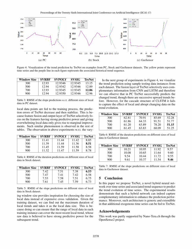
Figure 4: Visualization of the trend prediction by TreNet on examples from PC, Stock and GasSensor datasets. The yellow points representtime series and the purple line in each figure represents the associated historical trend sequence.


Table 3: RMSE of the slope predictions w.r.t. different sizes of localdata in PC dataset.

local data points are fed to the training process, the predic-tion errors of TreNet decrease and then stabilize. This is be-cause feature fusion and output layer of TreNet selectively fo-cus on the features having strong predictive power and givingoverwhelming local data only gives rise to marginal improve-ments. Such similar phenomenon is observed in the rest oftables. The observation in above experiments w.r.t. the vary-


Table 4: RMSE of the duration predictions on different sizes of localdata in Stock dataset.


Table 5: RMSE of the slope predictions on different sizes of localdata in Stock dataset.

ing window size provides inspiration for choosing the size oflocal data instead of expensive cross validation. Given thetraining dataset, we can find out the maximum duration oflocal trends and takes it as the local data size. This is be-cause doing so can ensure that the range of local data in eachtraining instance can cover the most recent local trend, whoseraw data is believed to have strong predictive power for thesubsequent trend.

In the next group of experiments in Figure 4, we visualizethe trend prediction using sample testing data instances fromeach dataset. The fusion layer of TreNet selectively uses com-plementary information from CNN and LSTM and thereforewe can observe that in PC TreNet successfully predicts thechanged trend, though there are successive upward trends be-fore. However, for the cascade structure of CLSTM it failsto capture the effect of local and abrupt changing data on thetrend evolution.


Table 6: RMSE of the duration predictions on different sizes of localdata in GasSensor dataset.


Table 7: RMSE of the slope predictions on different sizes of localdata in GasSensor dataset.

5 ConclusionIn this paper we propose TreNet, a novel hybrid neural net-work over time series and associated trend sequence to predictthe trend evolution of time series. The experimental resultsdemonstrate that such a hybrid network can indeed capturecomplementary information to enhance the prediction perfor-mance. Moreover, such architecture is generic and extendiblein that additional exogenous time series can be fed to TreNet.

AcknowledgementsThis work was partly supported by Nano-Tera.ch through theOpenSense2 project.


2278

References[Atsalakis and Valavanis, 2009] George S Atsalakis and Ki-

mon P Valavanis. Forecasting stock market short-termtrends using a neuro-fuzzy based methodology. Ex-pert Systems with Applications, 36(7):10696–10707, July2009.

[Ballas et al., 2015] Nicolas Ballas, Li Yao, Chris Pal, andAaron Courville. Delving deeper into convolutional net-works for learning video representations. arXiv preprintarXiv:1511.06432, 2015.

[Bao et al., 2014] Yukun Bao, Tao Xiong, and Zhongyi Hu.Multi-step-ahead time series prediction using multiple-output support vector regression. Neurocomputing,129:482–493, 2014.

[Bashivan et al., 2015] Pouya Bashivan, Irina Rish, Mo-hammed Yeasin, and Noel Codella. Learning represen-tations from eeg with deep recurrent-convolutional neuralnetworks. arXiv preprint arXiv:1511.06448, 2015.

[Chang et al., 2012] Li-Chiu Chang, Pin-An Chen, and Fi-John Chang. Reinforced two-step-ahead weight adjust-ment technique for online training of recurrent neural net-works. IEEE transactions on neural networks and learn-ing systems, 23(8):1269–1278, 2012.

[Chung et al., 2014] Junyoung Chung, Caglar Gulcehre,KyungHyun Cho, and Yoshua Bengio. Empirical evalua-tion of gated recurrent neural networks on sequence mod-eling. arXiv preprint arXiv:1412.3555, 2014.

[Donahue et al., 2015] Jeffrey Donahue, Lisa Anne Hen-dricks, Sergio Guadarrama, Marcus Rohrbach, SubhashiniVenugopalan, Kate Saenko, and Trevor Darrell. Long-term recurrent convolutional networks for visual recogni-tion and description. In IEEE CVPR, pages 2625–2634,2015.

[Guo et al., 2016] Tian Guo, Zhao Xu, Xin Yao, HaifengChen, Karl Aberer, and Koichi Funaya. Robust online timeseries prediction with recurrent neural networks. In 2016IEEE DSAA, pages 816–825. IEEE, 2016.

[Hammerla et al., 2016] Nils Y Hammerla, Shane Halloran,and Thomas Ploetz. Deep, convolutional, and recurrentmodels for human activity recognition using wearables.arXiv preprint arXiv:1604.08880, 2016.

[Hochreiter and Schmidhuber, 1997] Sepp Hochreiter andJurgen Schmidhuber. Long short-term memory. Neuralcomputation, 9(8):1735–1780, 1997.

[Lipton et al., 2015] Zachary C Lipton, David C Kale,Charles Elkan, and Randall Wetzell. Learning to diag-nose with lstm recurrent neural networks. arXiv preprintarXiv:1511.03677, 2015.

[Liu et al., 2015] Jiajun Liu, Kun Zhao, Brano Kusy, Ji-rongWen, and Raja Jurdak. Temporal embedding in convolu-tional neural networks for robust learning of abstract snip-pets. arXiv preprint arXiv:1502.05113, 2015.

[Malhotra et al., 2015] Pankaj Malhotra, Lovekesh Vig,Gautam Shroff, and Puneet Agarwal. Long short term

memory networks for anomaly detection in time series. InEuropean Symposium on Artificial Neural Networks, vol-ume 23, 2015.

[Mao et al., 2014] Junhua Mao, Wei Xu, Yi Yang, JiangWang, Zhiheng Huang, and Alan Yuille. Deep captioningwith multimodal recurrent neural networks (m-rnn). arXivpreprint arXiv:1412.6632, 2014.

[Matsubara et al., 2014] Yasuko Matsubara, Yasushi Saku-rai, and Christos Faloutsos. Autoplait: Automatic miningof co-evolving time sequences. In ACM SIGMOD, pages193–204. ACM, 2014.

[Sutskever et al., 2014] Ilya Sutskever, Oriol Vinyals, andQuoc V Le. Sequence to sequence learning with neuralnetworks. In Advances in neural information processingsystems, pages 3104–3112, 2014.

[Taieb and Atiya, 2016] Souhaib Ben Taieb and Amir FAtiya. A bias and variance analysis for multistep-aheadtime series forecasting. IEEE transactions on neural net-works and learning systems, 27(1):62–76, 2016.

[Venkatraman et al., 2015] Arun Venkatraman, MartialHebert, and J Andrew Bagnell. Improving multi-stepprediction of learned time series models. In AAAI, pages3024–3030, 2015.

[Vinyals et al., 2015] Oriol Vinyals, Alexander Toshev,Samy Bengio, and Dumitru Erhan. Show and tell: A neu-ral image caption generator. In IEEE CVPR, pages 3156–3164, 2015.

[Wang and Oates, 2015] Zhiguang Wang and Tim Oates. En-coding time series as images for visual inspection and clas-sification using tiled convolutional neural networks. InWorkshops at AAAI, 2015.

[Wang et al., 2011] Peng Wang, Haixun Wang, and WeiWang. Finding semantics in time series. In ACM KDD,pages 385–396. ACM, 2011.

[Wang et al., 2016a] Jiang Wang, Yi Yang, Junhua Mao,Zhiheng Huang, Chang Huang, and Wei Xu. Cnn-rnn:A unified framework for multi-label image classification.arXiv preprint arXiv:1604.04573, 2016.

[Wang et al., 2016b] Linlin Wang, Zhu Cao, Yu Xia, andGerard de Melo. Morphological segmentation with win-dow lstm neural networks. In AAAI, 2016.

[Yang et al., 2015] Jian Bo Yang, Minh Nhut Nguyen,Phyo Phyo San, Xiao Li Li, and Shonali Krishnaswamy.Deep convolutional neural networks on multichannel timeseries for human activity recognition. In IJCAI, pages 25–31, 2015.

[Yuan, 2015] Chao Yuan. Unsupervised machine conditionmonitoring using segmental hidden markov models. InAAAI, pages 4009–4016. AAAI Press, 2015.

[Zhao and Magoules, 2012] Hai-xiang Zhao and FredericMagoules. A review on the prediction of building en-ergy consumption. Renewable and Sustainable Energy Re-

views, 16(6):3586–3592, 2012.


2279

hybrid neural networks for learning the trend in time serieshybrid neural networks for learning the...

Documents