hydraulic and hydrologic aspects of flood-plain … · hydraulic and hydrologic aspects of...
TRANSCRIPT

Hydraulic and Hydrologic Aspects of Flood-Plain PlanningBy SULO W. WIITALA, KARL R. JETTER, and ALAN J. IfOMMERVILLE
GEOLOGICAL SURVEY WATER-SUPPLY PAPER 1526
Prepared in cooperation with the Commonwealth of Pennsylvania Department of Forests and Waters
UNITED STATES GOVERNMENT PRINTING OFFICE, WASHINGTON : 1961

UNITED STATES DEPARTMENT OF THE INTERIOR
STEWART L. UDALL, Secretary
GEOLOGICAL SURVEY
Thomas B. Nolan, Director
The U.S. Geological Survey Library has cataloged this publication as follows-
Wiitala, Sulo Werner, 191$-Hydraulic and hydrologic aspects of flood-plain planning, by Sulo
W. Wiitala, Karl R, Jetter, and Alan J. Sommerville. Washington, U.S. Govt. Print. Off., 1961.
V. 69 p. illus., maps, diagrs., profiles, tables. 25 cm. i(U.S Geological Survey. Water-supply paper 1526)
Part of illustrative matter colored, part in pocket.Prepared in cooperation with the Commonwealth of Peimsylvania Dept. of
Forests and Waters.
Wiitala, Sulo Werner, 1918-Hydraulic and hydrologic aspects of flood-plain planning. 1961.
(Card 2)1. Flood control. 2. Hydraulic engineering. I. Jetter, Karl R 1897- joint
author. II. Sommerville, Alan J joint author. III. Pennsylvania. Dept. of Forests and Waters. IV. Title. V. Title: Flood-plain planning. (Series)
For sale by the Superintendent of Documents, U.S. Government Printing Office Washington 25, D.C.

CONTENTS
PageAbstract_ _______________________________________________________ 1Introduction._ ____________________________________________________ 1Purpose and scope-________________________________________________ 3Hydraulic and hydrologic aspects..______-______-__-_-_-_-____-______ 3Phase I Flood-plain planning for a reach near a stream-gaging station. _ _ _ 5
Data available________________________________________________ 6Streamflow records.. ___-_________-__-_--_-_-______-_-___--___- 7Flood frequency.______-___________-_______________ -_________-_ 7Effect of bridges.____________________________________________ 13Stage-discharge relations_______________________________________ 14
Carnegie stream-gaging station_________-______---_________-_ 17Third Street Bridge__-___-_-_____-_____--____---___---_--_- 18Freight House Bridge__----_-------__--_--_---------_---__- 18Main Street Bridge--__------_----_-_---------_--_--------- 19Chestnut Street Bridge-..---.-----.------------------------ 19Turner Road Bridge.____-____________-____-_----_-_-----_- 19
Flood profiles-______________________________________________ 20Flood-plain map___-____________.____-____-____--__-____--__-_- 23Velocity---________-__-__-______-___-_-___--__--_-___----__--- 24
Phase II Flood-plain planning for a reach distant from a gaging station onthe same stream..___________________________________________ 27
Data available- _______________________________________________ 28Determination of discharge.__-_____________--_-__--_____-_---__ 29Flood frequency.--_________--__-_-__-__-_-_-_-___-_____--___-_ 30Effect of bridges__________--____-__-__-___-____--___---__-___ 31Stage-discharge relations. ______________________________________ 32
Section B...______________________________________________ 32Sections E and GL_________________________________________ 36Section /_________________________________________________ 36
Flood profiles.________________________________________________ 36Flood-plain map_____________________________________________ 37Velocity...___________________________________________________ 38
Phase III Flood-plain planning for a reach on ungaged streams. _______ 40Part 1. Discharge-frequency approach___________________________ 40
Field data available_____________._____---___-_____-_-_--__- 41Flood frequency.______----______-_____--_____-__--__--___- 42Effect of bridge.-:-________________-____--___-_-------_--_ 45Stage-discharge relations.__________________________________ 46Flood-plain map_________________________________________ 46
Part 2. Approach bypassing determination of discharge.__________ 48Data available. _________--______-___________-____--_--_--_ 48Flood frequency..____-----______-__________-____-_---__--- 49Stage-discharge relations. __________________________________ 49Correlation of flood depths with physical features of drainage area
and channel___________________________________________ 53Application of the simplified method________________-_------_ 54Discussion of results_-__-_-___________-_____-_-___-_______- 58
in

IV CONTENTS
Flood hazards._ _ ______Effects of urbanization. Zoning considerations.. Conclusions. __________Sources of data_______.Index,_______________
ILLUSTRATIONS
[Plates are in pocket]
PLATE 1. Flood plain of Chartiers Creek at Carnegie, Pa,.2. Flood plain of Chartiers Creek at Mayview, Pa.3. Profiles of Chartiers Creek at Carnegie and Mayview, Pa.4. Map of Pennsylvania showing location of gaging stations and
regions.
FIGUBE 1. Location of study sites, Allegheny County, Pa_____________2. Sketch of Chartiers Creek at Carnegie, Pa_________________3. Frequency of annual floods, Chartiers Creek at Carnegie, Pa.,
actual record.________________________________________4. Frequency of annual floods, Chartiers Creek at Carnegie, Pa.,
comparison with regional analysis________-___-_-___-__-5. Variation of mean annual flood with drainage area, Youghio-
gheny-Kiskiminetas River basins_______________--_-_-_-6. Cross section at Third Street, Chartiers Creek at Carnegie,
Pa___-__-__-________________________________________7. Cross section at Walnut Street, Chartiers Cre?k at Carnegie,
Pa__________________________________________________8. Stage-discharge relation for U.S. Geological Survey gaging
station on Chartiers Creek at Carnegie, Pa_ _____________9. Stage-discharge relations at Freight House, Main Street, and
Chestnut Street Bridges, Chartiers Creek at Carnegie, Pa_ _10. Relation of discharge and conveyance to sA,age at section
downstream from Turner Road Bridge, Chartiers Creek at Carnegie, Pa___________________________-__----__---_-
11. Cross section downstream from Turner Road Bridge, Chartiers Creek at Carnegie, Pa____-_---___--_-_----_-----------
12. West Main Street, Carnegie, Pa., flood of August 6, 1956_ _13. Frequency of average velocity at Walnut Street, Chartiers
Creek at Carnegie, Pa__________-____------___---------14. Sketch of Chartiers Creek at Mayview, Pa________________15. Frequency of annual floods, Chartiers Creek at Mayview, Pa__16. Relation of discharge, conveyance, and energ^ slope to stage
at section B, Chartiers Creek at Mayview, Pa____________17. Cross section at section B, Chartiers Creek at Mayview, Pa__18. Cross section at section B, Chartiers Creek at Mayview, Pa__19. Frequency of average velocity at section B, Chartiers Creek
at Mayview, Pa__________--___-__-_-__.--------------20. Plan-metric map of Pine Creek at Glenshaw, Pa___-________21. Profiles of Pine Creek at Glenshaw, Pa__-_-_-_--------_---22. Frequency of annual floods for streams in Allegheny County,

CONTENTS V
Page FIGURE 23. Variation of mean annual flood with drainage area for streams
in Allegheny County, Pa______________________________ 4424. Cross section, Pine Creek at Glenshaw, Pa_______________ 4625. Stage-discharge relation, Pine Creek at Glenshaw, Pa _______ 47
26. Relation of depth for mean annual flood and . , Pennsyl-D 1/3
vania streams._______________________________________ 55
27. Relation of depth for mean annual flood and ^ =^-. by regions,o 173
Pennsylvania. ______----__________--_____-___---_____ 56
2lation of depth for 10-year flood and l i by regions,D 1/3
Pennsylvania. ________---.-___-----_-_-_______-_______ 58-i/A/W
slation of depth for 25-year flood and v ' by regions,o 1 ' 3
Pennsylvania. _______________________________________ 59
A/A/Welation of depth for 50-year flood and v ' by regions,o 1 ' 3
Pennsylvania. _______________________________________ 60
TABLES
Page TABLE 1. Flood data, 1916-33, 1935, 1936, 1941-56, Chartiers Creek at
Carnegie, Pa__________________________________________ 92. Flood data, 1914-50, Chartiers Creek at Carnegie, Pa._______ 113. Computation of area and hydraulic radius at section B, C" artiers
Creek at Mayview, Pa__--______________________________ 344. Flood-profile data, Chartiers Creek at Mayview, Pa__________ 375. Computation of ratios, annual flood peaks to mean annual flood,
for area-frequency study--______-------_-___-____-______ 456. Pennsylvania stream-gaging station data____________________ 507. Comparison of results obtained by simplified indirect method
and the methods of phases I and II for selected cross sections on Chartiers Creek and Pine Creek, Allegheny County, Pa__ 57

HYDRAULIC AND HYDROLOGIC ASPECT? OF FLOOD-PLAIN PLANNING
By SULO W. WIITALA, KARL R. JETTER, and ALAN J. SOMMERVILLE
ABSTRACT
The valid incentives compelling occupation of the flood plain, up to and eve n into the stream channel, undoubtedly have contributed greatly to the develop ment of the country. But the result has been a heritage of flood disaster, suf- fering, and enormous costs.
Flood destruction awakened a consciousness toward reduction and elimination of flood hazards, originally manifested in the protection of existing developments. More recently, increased knowledge of the problem has shown the impractica bility of permitting development that requires costly flood protect/on. The idea of flood zoning, or flood-plain planning, has received greater impetus as a result of this realization.
This study shows how hydraulic and hydrologic data concerning the flood regimen of a stream can be used in appraising its flood potential and the risk in herent in occupation of its flood plain. The approach involves the study of flood magnitudes as recorded or computed; flood frequencies based1 on experience shown by many years of gaging-station record; use of existing or computed stage- discharge relations and flood profiles; and, where required, the preparation of flood-zone maps to show the areas inundated by floods of several magnitudes and frequencies.
The planner can delineate areas subject to inundation by floods o* specific recur rence intervals for three conditions: (a) for the immediate vicinity of a gaging sta tion; (b) for a gaged stream at a considerable distance from a gaging station; and (c) for an ungaged stream. The average depth for a flood of specific frequency can be estimated on the basis of simple measurements of area of drainage basin, width of channel, and slope of streambed. This simplified approach should be useful in the initial stages of flood-plain planning.
Brief discussions are included on various types of flood hazards, the effects of urbanization on flood runoff, and zoning considerations.
INTRODUCTION
The frequent occurrence of floods throughout the country, and the growing consciousness of the great damage and sufferng resulting from these floods, have aroused a widespread effort to reduce flood de struction. Failure to recognize that the natural function of a flood plain is to carry away excess water in time of flood, often has led to rapid and haphazard development on flood plains with a consequent increase in flood hazards.

2 FLOOD-PLAIN PLANNING
It is economically infeasible and often physically impossible to pro vide adequate flood-control measures for every locality subject to flood damages. Hence, corrective and preventive measures must be taken in order to adjust man's activities on flood plains to the regimen of streams. Such measures, generally known as flood-plain zoning or planning, can help solve or ease many flood problems.
Fundamental to effective flood-plain planning is the recognition of the flood potential of streams and the hazards involved in flood-plain occupation. Where necessary restrictions are imposed on communi ties in their flood-plain development, a marked reduction in flood damage is possible. Basic data on the regimen of the streams, par ticularly the magnitude of floods to be expected, the frequency of their occurrence, and the areas they will overflow, are essential to flood- plain planning.
The report was initiated through a cooperative agreement between the U.S. Geological Survey, Water Resources Division, and the Com monwealth of Pennsylvania, Department of Forest? and Waters. It was prepared under the direction of J. J. Molloy, district engineer, Surface Water Branch, U.S. Geological Survey, Harrisburg, Pa. The studies were made, and the report written, by S. W. Wiitala and K. R. Jetter, hydraulic engineers, U.S. Geological Survey, and by A. J. Sommerville, hydraulic engineer, Pennsylvania Department of Forests and Waters.
The provision in the Federal Flood Insurance Act of 1956, Public Law 1016, that involved consideration of flood-plain planning or zoning as a requisite for participation in the benefits of the Act, was the incentive for this study. Recognition of the need for such studies by the organizations involved in or proposing flood-plain planning in the Commonwealth provided further support.
Many of the data used in this report were collected over many years by the U.S. Geological Survey in cooperation with the Corps of Engineers, Department of the Army, and other Federal agencies, the Pennsylvania Department of Forests and Waters, and various public utilities. The data for the studies in phase III, pa.rt 2, and supple mentary field data for all phases were collected by tbe U.S. Geological Survey and the Pennsylvania Department of Forests and Waters.
All public and private authorities involved in flood-plain planning activities that were contacted for this report, cooperated by furnish ing data on the flood situation within their service areas. Additional data were obtained from local industries and organizations, State, county, and local government officials, and interested individuals.

HYDRAULIC AND HYDROLOGIC ASPECTS 3
PURPOSE AND SCOPE
The purpose of this report is to present the various forns of hydro- logic data and hydraulic studies required in flood-plain panning, the methods for obtaining such data, and their applicatior. It is in tended as a guide and working manual for individuals or agencies engaged in flood-plain planning.
Methods for zoning the flood plain are presented in this study which has been divided into three phases, based upon th? extent of the hydraulic and hydrologic data available. Phase I treats with a reach of channel where a river gaging station is located; phase II treats with a reach located at a considerable distance from a gaging station on the same stream; and phase III treats with a reach on an ungaged stream.
The procedures outlined are not necessarily applicable to all regions, such as some areas of the West where rivers frequently change their course. They are also subject to improvement and revision as more data and experience become available.
Because the procedures can be best illustrated by specif c examples, the following sections not only discuss methods but also explain the mechanics involved in each phase.
The stream reaches selected as examples of the methods outlined in this report are located in Allegheny County, Pa. (fig. 1).
HYDRAULIC AND HYDROLOGIC ASPECTS
Adequate flood-plain planning requires consideration of flood dis charges and their relative magnitudes, their expected frequency, the elevations reached, and areas covered by the floodwaters.
Methods of measuring flood discharges fall into three main classes: (a) by direct, or current-meter, measurements; (b) by indirect meas urements such as slope-area, contracted-opening, flow over dams and embankments, flow through culverts, and critical depth; and (c) by hydraulic computations based on channel characteristics, the so- called slope-conveyance method.
The methods covered in the first two classes are described in stand ard hydraulics textbooks, in U.S. Geological Survey Water-Supply Paper 888, "Streamgaging Procedure," and in circulars and pam phlets published by the U.S. Geological Survey. The slope-convey ance method, which is most frequently applied in this report, is described in subsequent sections.
A knowledge of flood frequency is necessary to relate flood-plain occupancy to the risks involved. Methods of flood-frequency anal ysis, usually based on statistical theories, are almost as rumerous as investigators in this field. Descriptions of diverse methods are scat tered throughout engineering flood literature, especially in Federal,

FLOOD-PLAIN PLANNING
INDEX MAP OF PENNSYLVANIA
FIGURE 1. Location of study sites, Allegheny County, Pa.
State, and local flood reports. The annual-flood method is used exclusively in this report. Regional flood-frequency analysis, which gives areal significance to flood data, is recommended over individual flood-record analysis wherever adequate data are available. Both methods are briefly described in this report.
The relation of stage to discharge the rating curve is a funda mental tool. At gaging stations it is developed empirically by cur rent-meter discharge measurements. At other locations it must be estimated from the physical characteristics of the channel and flood plain. Usually it is necessary to develop rating curves to represent the stage-discharge relation for several control points within a reach of stream channel.
The rating curve represents the relation of stage to discharge at a particular section. The flood profile is a continuous line representing the water surface for a given rate of flow. The preparation of a flood

REACH NEAR A GAGING STATION 5
profile enables one to transfer the line of intersection of the water and ground surfaces to a map that will then show the area ir undated by that flood. A map delineating the areas inundated by several floods, identified by their expected average frequencies, completes the hy- drologic and hydraulic analysis of flood-risk appraisal on flood plains.
PHASE I FLOOD-PLAIN PLANNING FOR A REACH NEAR A STREAM-GAGING STATION
The procedures used in this phase can be briefly summarized in four steps: (a) preparation of a flood-frequency curve for the site; (b) definition of stage-discharge relations, or rating curves, for key sections in the reach of channel to be zoned. Selection of key sections will often be guided by the effect of bridges or other channel con strictions in the reach; (c) determination of water-surface profiles within the project reach for floods of selected frequency; (d) prepa ration of flood-plain maps delineating the areas inundr-ted by the floods for which profiles were drawn.
A reach of Chartiers Creek at Carnegie, Pa. (fig. 2), illustrates the use of hydraulic and hydrologic data in flood-plain planning where stream-gaging records are directly available. Carnegie, a borough of 12,000 population, is about 5 miles southwest of Pitts burgh. Most of the borough is nestled in the relatively narrow valley of Chartiers Creek between steep hills rising above the flood plain on either side of the valley floor. The stream CMts through the central business section of the town and is a serious flood hazard. The flood plain is almost completely developed for industrial, com mercial, and residential uses. A large area adjacent to the stream channel has fallen into disrepair, possibly because of the frequently recurring floods.
Chartiers Creek flows northward through Carnegie r.nd empties into the Ohio River at McKees Rocks about 7 miles downstream. The topography of the drainage basin is rugged, generally typical of southwestern Pennsylvania. The stream-gaging station at the upstream borough limit (fig. 2) measures the discharge from 257 square miles of drainage area. Robinson Run, one of the larger tributaries, draining an area of about 40 square miles, enters Chartiers Creek a short distance upstream from the gaging station. Several smaller tributaries, Campbells Run, Whiskey Run, and Bell Run, enter the stream within the borough limits. These tributaries, because of their steep slopes and rapid runoff, have caused unex pectedly heavy damage along their immediate flood plains.
The reach of Chartiers Creek selected for study extends from the stream-gaging station downstream to Turner Road Bridge, a total river distance of 13,200 feet, or 2% miles. Ten bridgee, several of which are definite constrictions, span the stream within this length.

FLOOD-PLAIN PLANNING
Superior Steel Co NOT TO SCALE
FIGURE 2. Sketch of Chartiers Creek at Carnegie, Pa. (Stationing is in feet.)
DATA AVAILABLE
Gage-height and streamflow records covering 36 years are available for the project reach. The map of the reach (pi. 1) was prepared from a planimetric map of Carnegie borough (scale: 1 inch=300 feet) and a topographic map of the area downstream from the borough limits. Many floodmarks remaining from the record flood of August 6, 1956, were still easily recognizable. Much additional information on flood heights and the effect of flooding during that flood were obtained from local residents.
The following field data were obtained by a transit-stadia survey made for this study:1. Elevations of August 6, 1956,. floodmarks. Information of
crest heights of other floods was obtained in a few locations, but these data were mostly fragmentary and indefinite.

BEACH NEAR A GAGING STATION 7
2. Waterway openings at bridges.
3. Elevations of previously established reference points at all bridges.
4. Elevations of gage zero of discontinued gages at Freight House and Main Street Bridges.
5. Elevations of street and alley intersections in the flood area within the borough.
6. Cross sections of the stream channel at several locations.From the field measurements, profiles were drawn of the flood of
August 6, 1956, the low-water surface, the streambed, and the center- lines of streets leading toward the river.
STBEAMFLOW RECORDS
Flood stages and discharges were obtained from the records for the stream-gaging station at Carnegie, Pa. The gaging station was initially established on June 5, 1915, about 3,000 feet downstream from the present gage, at a site known locally as the Freight House Bridge. Annual peak discharges prior to September 30, 1919, were estimated from gage-height records. Daily discharges and annual peak discharges were obtained at this site from October 1, 1919, to December 15, 1931.
On January 8, 1932, the gage was moved to the Main Street Bridge, 1 mile downstream from the present gage, where discharge records were collected until September 30, 1933. Fragmentary records of gage heights were obtained until October 28, 1936, when the site was abandoned. The 1935 and 1936 annual flood peake were com puted from the fragmentary record. Discharge records were resumed November 20, 1940, at the present site upstream from the Superior Street Bridge and are continuous to date.
Because there is very little inflow between the three gage sites, the recorded peak discharges are equivalent.
FLOOD FREQUENCY
Gaging-station records provide the basic data for flood-frequency analysis. In phase I, an individual analysis was made to illustrate single-station procedures. The results of a regional flood-frequency study for an adjacent area were available for checking the consistency of the individual analysis. However, regional flood-frequency analysis should be considered for all flood-plain zoning studies. Where river records are short, it is even more important that the flood-frequency analysis be supported by regional experience.

8 FLOOD-PLAIN PLANNING
U.S. Geological Survey Circular 204, "Floods in the Youghiogheny and Kiskiminetas River basins, Pennsylvania and Maryland," outlines the procedures used and gives the results of a regional flood- frequency study. Regional flood-frequency methods have also been described by Tate Dalrymple. 1 Computation procedures for regional flood-frequency analysis are illustrated in phase III, part 1.
In this report, the annual-flood method of flood-frequency analysis is used wherein the maximum flood of each year is listed and the
AM-l plotting position is computed by the formula, RI= -^ ; where RI
is the average recurrence interval in years, N is the number of floods in the array, and M is the rank of the floods in descending order of magnitude. The points thus computed are plotted on a special prob ability graph paper devised by R. W. Powell to fit the statistical theory of extreme values as developed by E. J. Gumbel. On this graph paper, the frequency curve of annual floods should theoretically plot as a straight line. In actual practice, however, the curve is usually drawn to best fit the plotted points. For this reason, any graph paper on which the time scale is compressed at the upper end and expanded at the lower end will be satisfactory. The great ad vantage of the annual-flood method is its simplicity. The results are substantially equivalent, within any given period of record, to those obtained by several other methods.
Wherever possible, momentary peak discharges are used in flood- frequency analyses. Daily mean discharges may be adequate for some large rivers and for slow-rising streams with $, large proportion of their drainage areas in lakes and swamps, but for flashy streams, such as those in Pennsylvania, the momentary peak discharge is often much greater than the maximum daily mean. A frequency curve is not a rigid mathematical expression; it is simply a prediction, based on experience, of what is likely to happen. A frequency curve does not indicate when a certain event will occur; it is rather a means of estimating how often on an average, it will occur. It will change as additional records accumulate. Sampling errors are large in the short records available on most streams, making extrapolation uncertain. Although the flood-frequency curve is a very useful tool, the user should recognize its limitations.
The maximum annual floods, as recorded at the Carnegie gaging station, were first listed in table 1 by water years ending September 30. Information collected by the Chartiers Valley Flood-Control Committee indicates that a discharge of 12,000 cfs (cubic feet per second) was not exceeded in the period between the historical flood
1 Dalrymple, Tate, 1950, Regional Flood Frequency: Highway Research Board (Natl. Resources Council); Research Rept. No. 11-B.

REACH NEAR A GAGING STATION 9
TABLE l.~Flood data, 1916-83, 1935, 1936, 1941-56, Chartiers Creek at Carnegie, Pa.
[Drainage area, 257 square miles. Period of record, years of actual record]
Water year
1916 1917 1918 ..1919.... ..1920 ..
1921 1922.-....-.-..1923.... -..1924-... --..1925
1926 1927 1928 1929 1930
1931 1932 1933 1935 1936
1942 ..1943 1944 1945
1946.. 1947. ...1948. ..1949 ..1950 . -------
1951- 1952
1954 ..1955 ------1956..... ..
Date
Mar. 22, 1916 Jan. 22,1917 Feb. 26,1918 July 15,1919 June 17,1920
Sept. 21, 1921 Apr. 1, 1922 May 13,1923 June 29,1924 Feb. 7, 1925
Sept. 5, 1926 Nov. 16,1926 June 22,1928 Feb. 26,1929 Nov. 18, 1929
Apr. 4, 1931 Jan. 30,1932 Mar. 15, 1933 Aug. 7, 1935 Mar. 17,1936
June 5, 1941 Apr. 9, 1942 Dec. 30,1942 Mar. 7, 1944 Mar. 6, 1945
May 27,1946 June 8, 1947 Apr. 14,1948 Dec. 16,1948 July 5, 1950
Dec. 4, 1950 Jan. 27,1952 May 7, 1953 June 16,1954 Oct. 16,1954 Aug. 6, 1956
Gage height i
(feet)
11.1 12.0 7.4 8.11
16.1
11.5 9.61 8.5
10.1 6.0
11.3 10.50 12.22 12.2 9.2
10.03 4.8
10.0 6.85
11.0
6.85 11.00 12.30 8.88
13.49
6.14 8.33 8.94 6.86 9.41
11.31 10.33 7.07 8.08
11.55 16.37
Dis charge
(cfs)
2 6, 510 27,000 2 3, 020 23,590 32,800
36,950 35,000 33,950 35,500
2,050
36,560 35,650 37,660 37,660 34,280
35,100 2,390
38,200 24,260 39,600
3,090 7,380 8,700 4,850
12,200
2,270 4,280 4,920 2,960 5,100
7,160 6,000 3,030 3,890 7,520
13,500
Annual floods
Order(M)
15 12 32 29
2
13 21 27 18 36
14 17
7 8
25
20 34
6 26
4
30 10
5 23
3
35 24 22 33 19
11 16 31 28
9 1
Recur rence
interval (years)
2.46 3.08 1.16 1.27
22.50
2.84 1.76 1.37 2.06 1.03
2.64 2.18 5.29 4.62 1.48
1.85 1.09 6.17 1.42 9.25
1.23 3.70 7.40 1.61
15.00
1.06 1.54 1.68 1.12 1.95
3.36 2.31 1.19 1.32 4.12
45.00
Remarks
Corrected for ice backwater.
Estimated.
1 Referred to gage existing on date of peak; Inside gage after 1941.2 Computed for this report; not previously published.3 Revised for 1950 compilation report.
of September 1912 and the beginning of streamflow records at Car negie in June 1915. Because the floods of 1956, 1920, and 1945, were greater than 12,000 cfs, and thus greater than any since 1912, the recurrence intervals for these three floods were computed from
44+1the formula, RI M Recurrence intervals for the remaining
floods were based on the period of actual record (36 years) and were36+1computed from the formula, RI='
MThe computed points were plotted on the frequency chart (fig. 3),
and a smooth curve was drawn to average the plotted points. The curve shows that a flood equal to that of August 6, 1956, the greatest

10 FLOOD-PLAIN PLANNING
on record, can be expected to occur on an average of once in 37 years. The flood discharges used subsequently in this phase of the report were selected from the frequency curve shown in figure 3.
1.01 1.1 1.2 2 3 4 5 6 8 10
RECURRENCE INTERVAL, IN YEARS
30 40 50
FIGURE 3. Frequency of annual floods, Chartiers Creek at Carnegie, Pa., actual record.
To check this flood-frequency analysis, the relation of the Chartiers Creek data to that of the previously mentioned Youghiogheny- Kiskiminetas regional study, was investigated. The area covered by the regional study is only a few miles east of the Chartiers Creek basin. An analysis of Chartiers Creek flood data was made for the period 1914-50, the base period used in the regional study. The data listed (table 2) in parentheses show the estimated p-^aks on Chartiers Creek for 1914, 1915, 1934, 1937-40. These peak figures are not absolute and indicate only the approximate position of the estimated peaks in the array for the base period.
The resulting individual frequency curve (not shown) gives a value of 5,500 cfs for the mean annual flood at Carnegie. The mean annual flood, according to the theory of extreme values, is the flood having a recurrence interval of 2.33 years. The ratio of each annual flood to 5,500 cfs (table 2) was then computed and plotted versus recurrence

REACH NEAR A GAGING STATION 11
TABLE 2. Flood data, 1914-50, Chartiers Creek at Carnegie, Pa.
[Graphical mean annual flood (62.33) 5,500 cfs for period 1914-50. Drainage area, 257 sqrare miles. Period of record, 1916-33, 1935, 1936, 1941-50]
Water year
1914 1Q1 e
1916 1917
1918
1919 1920 1921 1922 1923
1924.- -19251926. 1927 1928.
1929 1930 1931 1932 1933
1934.
1935. .1936 1937. 1938
1939. . .1940.. 1941. .1942. .1943.
1944... .1945. - 1946 1947.-----.-..1948 _1949.- ___ ...1950 -
Date
Mar. 22,1916 Jan. 22,1917
Feb. 26,1918
July 15,1919 June 17,1920 Sept. 21, 1921 Apr. 1, 1922 May 13,1923
June 29,1924 Feb. 7, 1925 Sept. 5,1926 Nov. 16,1926 June 22, 1928
Feb. 26,1929 Nov. 18,1929 Apr. 4, 1931 Jan. 30,1932 Mar. 15, 1933
Aug. 7, 1935 Mar. 17,1936
June 5, 1941 Apr. 9, 1942 Dec. 30,1942
Mar. 7, 1944 Mar. 6,1945 May 27,1946 June 8, 1947 Apr. 14,1948 Dec. 16,1948 July 5, 1950
Gage height'
(feet)
ll.l 12.0
7.4
8.11 16.1 11.5 9.61 8.5
10.1 6.0
11.3 10.50 12.22
12.2 9.2
10.03 4.8
10.0
6.85 11.0
6.85 11.00 12.3
8.88 13.49 6.14 8.33 8.94 6.86 9.41
Discharge
Cfs
(4, 000)(6, 000)' 6, 510 > 7, 000
»3,020
> 3, 590 32,800 36,950 35,000 33,950
35,500 2,050
3 6, 560 3 5, 650 3 7, 660
37,660 3 4, 280 3 5, 100
2,390 38,200
(5,500)
»4,260 39,600 (6,600)(4,600)
(4,300)(4,600)3,090 7,380 8,700
4,850 12,200 2,270 4,280 4,920 2,960 5,100
Ratio to02.33
1.184 1.273
.549
.653 2.327 1.264 .909 .718
1.000 .373
1.192 1.027 1.393
1.393 .778 .927 .434
1.491
.774 1.745
.562 1.342 1.582
.882 2.218
.413
.778
.894
.538
.927
Annual Floods
Order (M)
(29) (14) 13 9
33
311
10 20 30
16 37 12 15 6
7 27 19 35
5
(17)
28 3
(11) (24)
(25) (23) 32
8 4
22 2
36 26 21 34 18
Re currence interval (years)
2.92 4.22
1.15
1.23 38.00 3.80 1.90 1.27
2.38 1.03 3.16 2.53 6.33
5.43 1.41 2.00 1.09 7.60
1.36 12.70
1.19 4.75 9.50
1.73 19.00 1.06 1.46 1.81 1.12 2.11
Remarks
Corrected for ice back water.
Estimated.
Observer noted peak Apr. 4.
1 Gage height referred to gage existing on date of peak; inside gage after 1941. a Computed for this report; not previously published. 3 Revised for 1950 compilation report.NOTE. Figures in parentheses were estimated by correlation with nearby stations and were used for
computation purposes only.
interval on figure 4. The regional curve for the Youghiogheny- Kiskiminetas basins, as contained in U.S. Geological Survey Circular 204, was plotted on figure 4 for comparison.
The Chartiers Creek data agree closely with the regional curve, indicating that Chartiers Creek is hydrologically comparable to streams in the Youghiogheny-Kiskiminetas region insofar as flood experience is concerned. Close agreement was also found between the frequency curve at Carnegie for the period of actual record (fig. 3) and a frequency curve in the regional study fo1* the period,
582753 O 61 2

12 FLOOD-PLAIN PLANNING
2.4
^ 2.0_i3
Z "
1
!"
CC
0.8
DA
^*> *n^*>
Yoifr
S*'
ghiogr equenc
" *~
sny a y cur
* *
id 1ve f
iskim vr peri
letai »dl<
X
rccional ( lA-50-^
/*
x/x
"1.01 1.1 1.2 1.5 2 34568 10
RECURRENCE INTERVAL, IN YEARS
20 30 40
FIGURE 4. Frequency of annual floods, Chartiers Creek at Carnegie, Pa., comparison with regionalanalysis.
MEAN ANNUAL (2.33-YEAR) FLOOD, IN CUBIC FEET PER SECOND
g w P .8 8 |
X/
/
/
/
/
/
/
sS
.< *
/.^/Char
x/
iers Cree
X< at Cam
/
gie, Pa.
10 20 50 100 200 ,510 1000 2000 50
DRAINAGE AREA, IN SQUARE MILES
FIGURE 5. Variation of mean annual flood with drainage area, Youghiogheny-Kiskiminetas Rive.basins, Pennsylvania.

REACH NEAR A GAGING STATION 13
1884-1950. Therefore, the frequency curve for the pericd of actual record at the gaging station is assumed to represent the longer period of record used in the regional study.
The graph of drainage area versus mean annual flood fo^ the period 1884-1950, developed in the regional study, is shown in figure 5. In the regional study, a factor of 1.076 was used for adjusting base- period (1914-50) mean annual floods to those for the longer period (1884-1950). Because the Carnegie frequency curves were analogous to those of the regional study, the same factor was used to adjust the mean annual flood at Carnegie (5,500 cfs) to the longer period. The adjusted point (5,920 cfs) is plotted on figure 5 for comparison.
EFFECT OF BRIDGES
The elevations of low steel (the lowest point of the superstructure of the bridge) and the sizes of effective waterway opening for 9 of the 10 bridges in the Carnegie reach are given in the following list. The Penn-Lincoln Parkway Bridge was omitted because its height and waterway area are so great that flood flows of the size considered in this report pass through it without constriction.
Elevation of low Effectivesteel (feet above waterway area
Bridge mean tea level) (square feet)Superior Street.--------___________________ 776.5 1,680Third Street-__--_-_-_-_____------------_--_--_ 772.9 1,650Railroad bridge No. 1________._____-____---- 776.4 1,930Freight House____-._-_____.________________ 775.5 1,960Main Street._______________________________ » 770. 8 1,320Chestnut Street.______________---_______._-__ 768.8 1,840P.O. & Y. Ry_.________________________________ 764.7 1,770Footbridge ______________________________ 765.3 1,600Turner Road______________________________ 763.0 1,930
i Top of arch.
Examination of the water-surface profile determined from the high- water marks for the flood of August 1956 (pi. 3) affords an excellent means of studying the effect of bridges on the flood flow in this reach of Chartiers Creek. The two-span concrete-arch bridge at Main Street appears to be a major channel constriction. The pier at mid stream is also conducive to lodgment of debris. A water-surface drop in excess of 1% feet through this bridge is evident at higher stages. The low steel of the Third Street Bridge alsc presents a high-water obstruction, but the smaller water-surface drop through the bridge is probably due to a ponding effect from the Main Street Bridge. Another large water-surface drop is shown fc1* the short reach of channel between the Pittsburgh, Chartiers and Youghiogheny Railway bridge and the footbridge. Because of a flood wall on the
14 FLOOD-PLAIN PLANNING
left bank and a factory building on the right, the floodwaters are funnelled through a narrow, constricted channel in this reach.
The profile for the flood of August 1956 (pi. 3) indicates that the bridges act as effective control points in the Carnegr'e reach. Hence, the project reach was subdivided into several subreaches, with bridges as control points, to better define the flood profiles.
STAGE-DISCHARGE RELATIONS
Rating curves describe the unique relation between the stage, (gage height) and the discharge, (rate of flow) commonly referred to as stage-discharge relation; they are of fundamental importance in all flood analyses. Because one curve is generally rot directly appli cable throughout a reach, it is necessary to develop auxiliary rating curves at control sections. These sections will usually be at points where breaks in the flood profile occur, such as at hrdges, at the head and foot of rapids, and at places where abrupt changes in channel characteristics occur.
At a stream-gaging station, the stage for a giver discharge is ob tained by reference to the station rating curve that is defined by dis charge measurements. Gaging-stations sites are se'ected at sections where a reasonably stable stage-discharge relation exists throughout the range of flow. Where the channel at a gaging-station site is subject to scour and fill, adjustment to the rating curve is readily made on the basis of the discharge measurements. However, the high-water part of the stage-discharge relation is relatively stable for most Pennsylvania streams and, when once defined, will be effective for long periods of time if the channel remains f~ee of man-made changes.
The base stage-discharge relation for the Carnegie reach is the rating curve for the stream-gaging station. To apply this rating curve throughout the reach, as required, it was necessary to supple ment the curve with auxiliary ratings developed by indirect means.
A simple and direct way of developing auxiliary rating curves is to establish temporary gages at the desired locations and read them during flood periods. These gage readings can tben be correlated with discharges at the stream-gaging station to produce the necessary rating curves. The timing of flood drift in a reach,, with appropriate adjustment of the observed velocity to the average, could produce rating curves for certain reaches. However, these procedures are time-consuming for completely defining high-water ratings and would rarely be used in flood-plain zoning studies.
Of the several different indirect methods of computing discharge mentioned on page 3 the slope-conveyance method is the simplest

REACH NEAR A GAGING STATION 15
to apply. This method is based on the Manning formula for flow in open channels which follows:
where
Q= discharge, in cubic feet per second.A= cross-sectional area of the channel in square feet,R= hydraulic radius in feet; defined as the cross-sectional area
divided by the wetted perimeter of the channel, in feet. n= a coefficient evaluating the roughness of the streambed and
banks. S= energy gradient, in feet per foot, which is dependent on the
stream slope and velocity distribution.If the first three terms on the right side of the Manning equation
are grouped together and called the conveyance, K, the equation then simplifies into the form, Q=KSl/2. All of the terms except n in the ex pression for the conveyance can be obtained from field measurements. The roughness coefficient must be based on judgment and experience, but tables and photographs are available in engineering literature from which reasonable selection can be made (such as King's "Hand book of Hydraulics," and other hydraulics textbooks). When the discharge for a particular stage is known, it is possible to compute an n that may be applicable over a large range of stage. A computa tion for the overflow section at Third Street is shown beT ow figure 6.
In applying the slope-conveyance method, it is helpful to compute the conveyance at selected elevations over the desired range of stage and draw a stage-conveyance curve. By combining conveyances from this curve with energy slope in the equation, Q=KF1/2, auxiliary rating curves may be obtained. At sections subject to overbank flow it is good practice to subdivide the valley cross section into subchannels whose relative conveyances differ because of different values of channel roughness and hydraulic radii. It is the practice of the U.S. Geological Survey to subdivide a valley cross section into roughly trapezoidal subchannels. The total conveyance for a cross section is equal to the sum of the conveyances for the various sub channels.
Certain assumptions must be made regarding the energy-gradient term. Experience has indicated that for the higher stages, the energy slope tends to become constant, and approaches the average slope of the streambed in unconstricted channels. Occasionally one or more floodmarks, with corresponding discharges, can be determined and the energy slope computed from the formula, S= (Q/K) 2 (see sample computation below fig. 7).

16 FLOOD-PLAIN PLANNING
/ io
776
UJ
ut 774z
772
770
1 1 1 1 1 1 luj 1 1 | | 1
K 3 2 3 /uj 2 v. 2 /
Ife >. " ^ § ^ * /
~ I 2 !S * i ° ^ ^/- I i ^ £ ^ « ^ c /
1 T i i i i i i /
^*^ __ _/ -" "" Left bank
1 1 1 1 1 1 1 1 1 1 1
1
Mainchannel
L-_
c~
S_£E
1300 1200 1100 1000 900 800 700 600 500 400 300 200 100
HORIZONTAL DISTANCE, IN FEET
FIGURE 6. Cross section at Third Street, Chartiers Creek at Carnegie, Pa. Computation of averagevelocities is as follows:
Computation of average velocity, Third Street overflow
Stage (feet
above mean sea
level)
776.5775.5774.5773.5
Section
_do-_ - -.do..-- --- -.do.... - ---
71
0.077.077.077.077
1.48671
19.319.319.319.3
R(feet)
3.822.932.021.06
Rtn
2.452.051.601.04
S (feet per
foot)
0.00073.00073.00073.00073
Si/a
0. 0270.0270.0270.0270
Average velocity (feet per second)
1.281.07.83.54
Computation of n used in above table:Overflow measured August 6, 1956, on Third Street (measurement 197)
= 3,211 cfs, water-surface elevation=775.5 feet. S=0.00073 measured from profile of flood of August 6, 1956 (pi. 3).
.(?0verflow_ 3,211
V0.00073K for overflow section= 8 L "
K_ 1.486 AR2/3 or 1-486n ' °r n~ K
A = 3,007 square feet (measured at time of measurement 197). .R = 2.93 feet, hydraulic radius computed for overflow, measurement 197. n== 1.486X3007X2.932 / 3 =()077 for overflow section> Third Street.
119,000
Where several such points over a large range of stage are available, a stage-slope curve can be drawn from which the slope term in the equation, Q=KSl/2 , can be evaluated. Where only one floodmark and corresponding discharges are available, the slope may be assumed constant and equal to that computed for the one point. These assumptions are valid only when the flood flow is not complicated by variable backwater. For example, the presence of debris jams in, or downstream from, a reach, or ponding effect from a downstream tributary or mainstream in flood, could cause variations in slope not definable by a few floodmarks not covering the full range of possible conditions.
In the Carnegie reach, the gaging-station rating curve is assumed to represent channel conditions to Third Street Bridge. Rating curves for the downstream sides of the Freight HoMse, Main Street,

REACH NEAR A GAGING STATION 17
400 500 700 900
HORIZONTAL DISTANCE, IN FEET
FIGURE 7. Cross section at Walnut Street, Chartiers Creek at Carnegie, Pa. Compt tation of averagevelocities is as follows:
Velocity computations
Stage (feet
above mean sea
feet)
770.3
769.5
768.5
767.5
766.5
765.6
Section
Right. . ...
Right. .
Right-
Right-
Right. .
n
0.035.077.035.077
.077
.035
.077
.077
.035
1.486 n
42.41Q °.
42.4
42.419 342.41Q °.
42.419.342.4
R(feet)
11 642 on
11.08i 04
10.411 439 fii
Q1
8 77
.40ft ne
Rl
5 151.744.981 %f\
4.751.274.53
94i 9H
.54
S (feet per
foot)
0 000973AAAQ7Q
flflflQ7^nAnQ7q
ft,AnQ7Q
nAnn'TQAAAQ7Q
AAAQ»yq
AAAQ7Q
nAAQ7Q
AAAQ'TQ
fi*
O AQ-t onqionoionqio
.0312nqio
.0312nqionqio
.0312
Average velocity (feet per second)
6 89
1.056 en
90c 97
.76
.575.63.33
5 01
Computation of slope:
.51X 1714=374,500.
#overbank= 19.3X1.74X1706=57,200; #Totai = 375,500+ 57,200- 43 1,700.
S*=|:=^j^=0.0312; 5=0.000973 for stage 770.3 (1956 peak).
and Chestnut Street Bridges are assumed to represent conditions for the reaches immediately downstream from them. The rating curve developed for a section 250 feet downstream from the Turner Road Bridge is assumed to represent conditions in the subreach farthest downstream.
CARNEQIE STREAM -QAQINQ STATION
Most recording stream-gaging stations are equipped with gages inside and outside of the gage wells. The rating curve for the Car negie gaging station (fig. 8) was referred to the outside gr.ge because that gage is more directly related to degree of flooding. To simplify construction of the flood profiles, gage heights were converted to elevation above mean sea level in the preparation of figure 8. A

18 FLOOD-PLAIN PLANNING
o 765
Gage heights referred to outside gage Discharge measurement
1000 2000 5000
DISCHARGE, IN CUBIC FEET PER SECOND
10,000 20,0^
FIGURE 8. Stage-discharge relation for U.S. Geological Survey gaging stat'on on Chartiers Creek aCarnegie, Pa.
stable stage-discharge relation is indicated for the present site. Dis charge measurement 197, made during the flood of August 1956, showed backwater of about 0.7 foot due to debris accumulated at the Superior Street Bridge during the flood. Therefore, the same degree of flooding downstream from Superior Street could be expected when the gage registers 0.7 foot lower stage and the bridge opening is unobstructed by debris.
THIRD STREET BRIDGE
The high-water discharge measurements for the stream-gaging station are usually made from the Third Street Bridge, and are referred to a point of known elevation on the bridge. These have been used to develop a rating curve (not shown) fc^ a section at the upstream side of Third Street Bridge.
FREIGHT HOUSE BRIDGE
Short extensions of the water-surface profiles defined by water- surface elevations at the gaging station and at the Third Street Bridge, were made to determine stages at the downstream side of the Freight House Bridge for several discharges. The points used, and the rating curve defined, are shown in figure 9. The ftage for the flood peak of August 6, 1956 (13,500 cfs) was taken from the water-surface profile defined by the survey of floodmarks.

REACH NEAR A GAGING STATION 19
3000 5000 10,000 2000 3000 5000
DISCHARGE, IN CUBIC FEET PER SECOND
10,000
FIGURE 9. Stage-discharge relations at Freight House, Main Street, and Chestnut Street Bridges, Chartiers Creek at Carnegie, Pa.
MAIN STREET BRIDGE
The rating curve for the old gage at Main Street was revised upon the basis of the profile data for the flood of August 6, 1956. The revised curve, also shown in figure 9, is applicable to the downstream side of the Main Street Bridge.
CHESTNUT STREET BRIDGE
A water-surface elevation, measured from a reference point at the Chestnut Street Bridge, was determined for the discharge measure ment of 3,310 cfs on April 5, 1957. Using this point and the peak for the flood of August 6, 1956, as indicated by floodmarks, a rating curve (fig. 9) for the downstream side of the Chestnut Street Bridge was estimated.
TURNER ROAD BRIDGE
The slope-conveyance method was used to compute a rating curve for a section 250 feet downstream from the Turner Road Bridge. All the flow is confined to the channel at this point. A cros-s section of the stream was obtained, and the elevation of the flood crest of August 6, 1956, was extrapolated from the profile defined by flood- marks farther upstream. The energy slopes for the flood of August 1956 (13,500 cfs), and the low flow of May 3, 1957 (25C cfs), were computed from the equation, S=(Q/K) 2 , giving results of 0.00120 and 0.00121 feet per foot, respectively. The slope of the streambed from the footbridge to Turner Road was obtained from the survey

20 FLOOD-PLAIN PLANNING
profile as 0.00118. Therefore, an average slope of 0.00120, anc conveyances taken from a stage-conveyance curve (fig. 10), wer
CONVEYANCE, IN THOUSANDS OF UNITS
WATER-SURFACE ELEVATION ABOVE MEAN SEA LEVEL, IN FEETVI VI VI. VI VI VI V Ol <J1 Ul CJI 0* 0* C ro *> o> oo O M *
1
X
/
X
J
/
\
X
X^
x>N
/^
\
i
'
\
i
\1 46 8 10 12 14 1
DISCHARGE, IN THOUSANDS OF CUBIC FEET PER SECOND
FIGURE 10. Relation of discharge and conveyance to stage at section downstream from Turner Roa( Bridge, Chartiers Creek at Carnegie, Pa.
used to compute the rating curve (fig. 10) from the formula, Q=KS1/2 Computations of conveyance and discharge are shown below figure 11 Detailed computation procedure for the section properties, area anc hydraulic radius, is illustrated in phase II (table 3).
FLOOD PBOFILES
The water-surface elevation in a pond, or other stationary wate body, is the same over its entire surface, but the water-surface elevation in a stream slopes in the direction of flow. The line showing the sloping water-surface elevation in a reach of stream for a given rat of flood flow is called the flood profile. The water-surface elevatior for the given flow rate can be ascertained for any location within the reach covered by the profile. Flood profiles provide a potent tool fo. studying the effect of bridges and other channel obstructions on flooc flows and also enable the appraisal of flood hazard for a particula

REACH NEAR A GAGING STATION 21
765
762
759
756
753
750
744
Left bank Right bank
20 40 60 80 100 120 200
HORIZONTAL DISTANCE IN FEET
Computation of conveyance and discharge
Stage (feet)
763.0761.0759.0757.0755.0763.0
Section
- do... ......- do. ....... . -do. ...... .... do......... -do.........
n
0.035.035.035noc
.035
.035
1.486 n
A<) A
42.4
A (square feet)
1 QflQ
1 641
1,106866OAA
R(feet)
11.009,868 fin
RM
A QK
4 604.20
K
'3AA ftfirt
1Q7 fwi138,00088,600
8 (feet per
foot)
.00120
00120.00120.00120
£1/2
.0346
.0346
Q (Cfs)
14,150
9,2106,820
3,070
FIGURE 11. Cross section and computation of conveyance and discharge downstream from Turner Road Bridge, Chartiers Creek at Carnegie, Pa.
piece of property by comparing ground elevations at the site with the profile elevation for that section of stream.
The best and most direct determination of the water-surface pro file in a reach is by the survey of the actual marks left by a flood at its peak. Well-defined high-water marks can be obtained by identifying the points in the field immediately after a flood has receded. Later, well-preserved high-water marks can be found inside buildings that were flooded. Some local residents mark the elevations of outstanding floods on their property and a survey of such marks can yield valuable data for the construction of flood profiles. Most of the time, however, the flood-plain planner will be confronted with scarce, rather than abundant data. In isolated reaches, particularly a long time after

22 FLOOD-PLAIN PLANNING
a flood, floodmarks must be identified from debris caught in the limbs and bark of trees, from dried-out wash lines, from twigs and grass washed on the banks by eddies or deposited in slack water, or from less obvious signs that are recognizable only to those experienced in such observations. Such floodmarks must be used with caution and selected to be consistent among themselves.
For the Carnegie reach, flood lines representing recurrence inter vals of 50, 37, 25, 15, 10, 5, 2.33, and 1.5 years are shown on plate 3. The discharges obtained from the flood-frequency curve (fig. 3) are applicable throughout the reach and are as follows:
Recurrence interval JDischarc" (years) (c/s"
50___-_--____-_ -_____--_----__--_-_-_---___________________ 14, 50C37 (flood of Aug. 6, 1956)__._.-_.----__----_--_.... -_.-.-______._ 13, 50C25._____________________________________________________________ 12, 30C15--------__------------_----_----_---------_-__-___----_----___ 10, 90C10_--_____-___-_-__--_-____--____--__-__-___-_____-_____________ 9, 80C5.----_---___----_----_------------------_----__-_-------_----__ 8, OOC2.33 (mean annual flood) _-___-__.-__-_.---___--_____-__.-__---__-_,__ 5, 80C1.5 (about bankfull flow) ___-___---______-__--_______-______-______ 4, 40C
The profile for the flood of August 1956 in Carnegie was defined by the field survey of floodmarks. Profiles for the other floods were determined by dividing the reach into subreaches, each having a key section for which a rating curve was available or computed The stages of specific discharges at the key sections were obtained from the rating curves, and lines emanating from those points were drawn, making certain assumptions regarding slope as discussed below:1. Upstream from Third Street Bridge, lines for the 50-, 25-, 15-
and 10-jTear floods, all above low steel of the bridge, were drawn parallel to the profile for the flood of August 6, 1956. For the smaller floods, the profiles were drawn parallel to the water- surface slope prevailing at the time of discharge measurement 123 (6,450 cfs).
2. All profiles in the two reaches, Freight House Bridge to Mair Street and Main Street to Chestnut Street, were drawn paralle to the profile of the flood of August 6, 1956.
3. Between Chestnut Street and the Pittsburgh, Chartiers anc Youghiogheny Railway bridge, the 50-, 25-, and 15-year flood profiles were drawn parallel to that for the H 56 flood. Profile? of the smaller floods were drawn parallel to the slope of the streambed between stations 7,000 and 9,OOC. River distance in feet, measured from the upstream end of the reach undei consideration is used here, on plates 1 and 3, and subsequently in figure 21 and on plate 2. High-water marks for the floods
REACH NEAR A GAGING STATION 23
of June 1920^(12,800 cfs), July 1943 (7,310 cfs), and March 1945 (12,200 cfs), check the profiles as drawn within about half a foot.
4. Downstream from the railroad bridge, profiles for floods having recurrence intervals of 10 years or more were drawn parallel to the profile for the 1956 flood. Profiles for the smaller floods were drawn parallel to the streambed.
FLOOD-PLAIN MAP
A map showing the areas inundated by floods of various frequencies is the result of this study. On each bank, lines enclosing the flooded area for any particular flood were drawn by transferring elevations from the appropriate water-surface profile to the map. Elevation contours, if available on the map, were used as guides in drawing these flood lines.
For flood-zoning studies, the base maps used for the preparation of the flood-plain maps should show topography and should be of sufficiently large scale to show abundant detail. Maps of this type that cover flood plains are not generally available hence, the investi gator will have to make his own topographic survey, or improvise by supplementing the best available maps with field-survey data. For the Carnegie map (pi. 1), the position of the flood lines downstream from the borough limits could be determined with fair accuracy using topographic maps of that area as a base. Within the borough, how ever, where no topographic map was available, the position of the flood lines was determined by spotting the water-surface elevations taken from the flood profiles at the corresponding points on the streets leading toward the river and then transferring these points to plate 1. On plate 1, the flood lines have been identified w: th the gage height at the gaging station for the discharge corresponding to the flood line. This procedure ties in all the flood lines in a reach to one gage and permits estimation of the depth of floe ding. The location and spacing of the flood lines also shows the extent and approx imate rate at which depth of inundation changes.
A concrete flood wall on the left bank extends from the Ryerson Steel Co., station 9,000, to the sharp bend at station 12,000. Com parison of the elevation of the top of the floodwall with the flood profiles indicates that upstream from the Pittsburgh, Chartiers and Youghiogheny Railway bridge, the floodwall is overtopped by floods having a recurrence interval of 15 years or more. When this happens, the area on the left bank upstream from the railroad beccmes a large pool because there is no outlet through the railroad embankment, and remains flooded until drained by seepage and evaporation. Downstream from the railroad bridge the floodwall is overtopped only by floods having a recurrence interval of 25 years or more.

24 FLOOD-PLAIN PLANNING
Exact delineation of flooded areas is practically impossible and i. not warranted for most studies. Where precise definition of floodet areas is required, very detailed field surveys must be made. How ever, the flood-plain map (pi. 1), as prepared, serves its primary purpose of giving a general picture of the area in Carnegie subjec to inundation by Chartiers Creek and the expected frequency of sue1 inundation.
Except in the downstream areas subject to br.ckwater from th main stream, floods on the small tributary streams are usually inde pendent entities as to frequency and area of flooding. The are/ inundated by the flood of August 6, 1956, on Campbells Kun is show on plate 1 by a dot-dash line. Areas inundated by other floods along this or other tributary streams, are deterninable by studie; similar to those described on page 23.
VELOCITY
In appraising the damage potential on a flood plain, the flood plain planner must consider the magnitude and location of the veloc ities to be expected. The moving stream of water is frequently th principal cause of damage in places where simple inundation is merer; a nuisance. High velocities can damage or destroy bridges, embank ments, and paving; undermine and collapse buildings; pile up debri. and transport sediment and gravel, often to slack water wher damaging deposits are formed; and erode areas of land. Abrasiv damage is increased when flowing water carries in suspension a heav; load of gritty material. In flowing down a flood plain, floodwate piles up against buildings or other obstructions in its path with con sequent acceleration and concentration of flow around the corner (fig. 12). At such points, scouring action on the ground supportir" the structure, and even on the structure itself, is greatly increased Scouring action, usually confined to areas contiguous to the strear channel and around obstructions on the flood plair, may cause majo flood damage, especially on streams with steep slopes.
The effect of high velocities frequently complements the effec of inundation. This is dramatically evident wh°,re high velocitie, transport structures to their eventual destruction after the structure have first been loosened from their foundations by the buoyan effect of deep inundation. Where a large part of the flood flow i out of a stream's normal meandering channel, the floodwaters see1 the most direct passage through a reach, thus reducing the distanc traversed and increasing the slope and velocity. The inducec velocities may be high enough to scour cutoffs and new channels.
Besides the depth of inundation and magnitude of the velocity the effect of other factors must be assessed in attempting to ascertaii

REACH NEAR A GAGING STATION 25
MElLOf BANK
FIGUKE 12. West Main Street, Carnegie, Pa., flood of August 6, 1956. Photograph supplied by the"Carnegie Signal Item."
the scouring action of streams in flood. The direction of the current, type of material supporting structures, and the design, size, condition, and location of structures are some of the most important elements. Any one, or a combination, of these may sometimes produce critical damage. Success in providing adequate scour protective measures is a matter of experience and judgment in appraising all of the condi tions at a particular site.
It is very difficult to make accurate quantitative estimates of flood velocities. Average velocities can be computed from op Qn-channel flow formulas, such as the modification of the Manning formula,
1 486 V= R2/*Sl/2, and from the relation, V QjA, when the discharge
71
and cross-sectional area are known. Velocity computations for the Third Street and Walnut Street sections using the Manning formula are illustrated in figures 6 and 7. In figure 13, the average velocities computed for the main channel and overbank portions of the Walnut Street section are related to expected frequency of occurrence.
In defined channels the average velocity is indicative of velocities that may reasonably be expected and is therefore a meaningful quantity. Point velocities ordinarily are not more than 1^ to 2

26 FLOOD-PLAIN PLANNING
771
770
§ 768
< 766
765
RECURRENCE INTERVAL IN YEARS
15
Right overbank Main channel
AVERAGE VELOCITY, IN FEET PER SECOND
FIGURE 13. Frequency of average velocity at Walnut Street, Chartiers Creek at Carnegie, Pa.
times greater than the average in defined channels. On the othe hand, the average velocity on the flood plain provides a very uncertar clue to velocity distribution. Because there are so many irregu larities and obstructions on the flood plain, and because these ar subject to frequent change, quantitative predictions of velocity r specified locations on the flood plain are almost impossible to make It is only possible to make qualitative deductions, such as, tha maximum velocities usually occur in the deepest parts of a cross sec tion and where there is least resistance to flow, as along streets ar alleys.
Current-meter measurements of overbank flow provide excellen data on velocities on the flood plain. However, such data are availabl only for selected locations where discharge measurements are, or hav been, made. A current-meter measurement of overbank flow crossirv Third Street in Carnegie was made a few hours after the crest of th flood of August 6, 1956. Maximum measured point velocity was feet per second at the intersection of Third Street and Third Avenue The average velocity for this overbank section was slightly greate than 1 foot per second. At this section, maxirrum point velocity

REACH DISTANT FROM A GAGING STATION 27
was four times greater than the average. Hence, for overbank sec tions having physical characteristics similar to those of the Third Street section, a maximum point velocity of about four tines the com puted average velocity could be expected.
Average and maximum velocities of 1 and 4 feet per second, re spectively, for an overflow section would not cause serious1 scour in an unobstructed cross section. However, velocities of 4 feet per second in depths of 3 feet or more might easily sweep persons off their feet, thus creating a definite drowning hazard. Where the passage of overflows is more seriously restricted, point velocities on the'order of 7 to 10 feet per second could reasonably be expected. Velocities of this magnitude could definitely cause scour leading to failure of build ing foundations.
PHASE II FLOOD-PLAIN PLANNING FOR A REACH DISTANT FROM A GAGING STATION ON THE SAME STREAM
Where a reach of river is some distance away from the primary source of the required hydraulic and hydrologic data, the flood-plain planner is faced with two problems. The first is the determination of flood discharges at the site, and the second involves the definition of stage-discharge relations for the required sections within the reach un der consideration. Both problems require solution by indirect methods. Flood discharges are determined by finding some means of transferring the flood experience of a gaging station to the site. Stage-discharge relations can then be estimated from an analysis of the physical characteristics of the channel and flood plain, abetted by whatever floodmarks that can be identified for known floods, by the methods already described.
After the magnitude and frequency of floods have been determined and the stage-discharge relations established, the procedures follow those described in phase I for drawing water-surface profiles, com puting velocities, and delineating on a map the flood areas for floods of specific frequency.
The reach selected for illustration of procedures for obtaining and applying the hydraulic and hydrologic data involved in flood-plain planning under phase II is on Chartiers Creek about 12 mil°,s upstream from Carnegie, Pa. The reach extends from Boyce Eoad Bridge downstream to Mayview Eoad Bridge, a river distance of about 2% miles (fig. 14). Mayview State Hospital is on the left bank within this reach.
The entire flood plain is a flat, undeveloped area of f 3lds with a fringe of brush and woods adjoining the stream. At the upper end of the reach, flood plains are on both sides of the stream; in the lower
582753 O 61 3

28 FLOOD-PLAIN PLANNING
Station 12.0OO
NOT TO SCALE
FIGURE 14. Sketch of Chartiers Creek at Mayvlew, Pa. (Stationing is in feet.)
half, steep, high hills rise abruptly from the river along the right bank. A railroad bridge and a secondary-road bridge span the stream about three-quarters of a mile downstream from the Boyce Road Bridge. The drainage area at Boyce Road Bridge is 157 square miles, or 61 percent of the drainage area at the Carnegie stream-gagingstation.
DATA AVAILABLE
A 1925 topographic map of the area downstream from the railroad bridge, prepared for the development of the hospital rHe, was used as a base map in the drafting of plate 2. Use of this map was believed justifiable because practically no development of the flood plain in this area has taken place since 1925. Differences between the 1925 map and existing conditions were noted during the course of field work on this project and, where the differences were significant, adjustments were made on plate 2. The field survey (1957) al^o indicated that
REACH DISTANT FROM A GAGING STATION 29
0.5 foot must be added to all elevations on the 1925 map to convert them to present sea level datum. For the area upstream from the railroad bridge, the map was prepared from the field-survey data obtained for this report. Elevations in the field were referred to present sea level datum and were adjusted to the 1925 map datum before transferring them to plate 2.
The following information was obtained from the transit-stadia field survey (1957):1. Stream-channel and flood-plain cross sections, including water-
surface elevations, at four sections upstream from the railroad bridge.
2. Stream-channel cross sections with water-surface elevations at five sections downstream from the railroad bridge. The flood-plain part of these cross sections was obtained from the topographic map.
3. Waterway openings of the four bridges.4. Elevations of the August 6, 1956, floodmarks. Few reliable
floodmarks could be found except near the ends of the reach.5. Estimates of roughness coefficients.
From these data, the profiles of the streambed and low-water surface were plotted for the reach. Identifiable high-water marks from the flood of August 1956 were scarce. The profile for this flood could be established from floodmarks only in the reach upstream from the railroad bridge, below this point it was drawn as described on page 37. Locations of the cross sections surveyed are shown in f^ure 14 and on plates 2 and 3.
DETERMINATION OF DISCHARGE
Estimates of discharge for the ungaged site based on discharge records at the gaging station can be made in several ways.
A direct way is to make a series of discharge measurements over the medium- and high-water range of discharge at the ungaged site. Direct comparison can then be made with the corresponding dis charges at the gaging station to define the discharge relation empiri cally. However, this comparison is usually difficult because the measurements at the ungaged site should be made at, cr near, flood crests to avoid the distorting effect of changing discharge in the reach between the two points. Flood events rarely happen by design so that application of this procedure may take a long time and delay flood-planning studies for areas requiring immediate attention.
Discharges for specific floods at the ungaged site can also be com puted by the slope-area method, or by one of the other methods of indirect measurement previously mentioned. These methods

30 FLOOD-PLAIN PLANNING
also involve much fieldwork and time and would rarely be practical for flood-zoning purposes.
The quickest and simplest procedure is to relate peak discharge to drainage area. Experience indicates that, for sites on the same stream, the discharge ratios are directly proportional to the drainage- area ratios raised to some power less than one. This may be ex pressed as,
m FAT L«J UJ
where Qi and AI= discharge and drainage area at the ungaged site; $2 and A2 = discharge and drainage area at the gaged site; and z=an exponent less than one, usually between 0.5 and 0.8. The value of the exponent can be estimated from the slope of a graph showing the relation between mean annual flood and drainage are 01 , for the drainage basin or region.
For a site between two gaging stations on the same stream, the discharges may be interpolated on the basis of drainage area from peak discharges recorded at each station.
The close agreement of the Chartiers Creek flood data at Carnegie with the data for the Youghiogheny-Kiskiminetas region has already been noted. Hence, the slope of the graph of the relation between mean annual flood and drainage area (fig. 5) determined in the regional study is applicable to the Chartiers Creel' basin. Because the exponent x in the discharge-drainage area relation in the regional study is 0.8 (the slope of the graph in fig. 5), the relation for Chartiers Creek can be expressed as,
L&jTL^cwhere A and Q refer to drainage area and discharge, and subscripts refer to Carnegie and May view. Solving by substituting the drain age area figures, QM=O.Q75QC .
FLOOD FREQUENCY
The flood-frequency curve for the May view rer.ch (fig. 15) was obtained simply by multiplying discharges taken from the Carnegie frequency curve (fig. 3) by 0.675. By this procedure, a discharge of 9,100 cfs at May view was computed for the flood of August 6, 1956 (recurrence interval of 37 years). Slope-conveyance computations for subreaches B-C and C-D, and a rough contracted-opening calcula tion for the Boyce Road Bridge section, check the discharge of 9,100 cfs within 10 percent.
The discharge-drainage area relation was used to estimate the flood-frequency curve in this phase of the study to illustrate its

REACH DISTANT FROM A GAGING STATION 31
DISCHARGE, IN THOUSANDS OF CUBIC
FEET PER SECOND
ON) * O> OB C
^
^
1
^
^̂ Curve
stati for p
1 1
^^^
:omputed frorr on on Chartiers *riod 1916-33
1 1
^x^
flood data \^' gaging Creek at Carr««ie, Pa., 1935, 1936, 1941-56
1 1.01 1.1 1.2 1.5 2 3 4 5 6 8 10 70 30 40 9
RECURRENCE INTERVAL, IN YEARS
FIGURE 15. Frequency of annual floods, Chartiers Creek at Mayview, Pa.
development and simple application. Where the project reach is near the gaged point on a stream, this method should give reliable results. However, if a statewide, or even a regional flocd-frequeiicy study is available, it would be better to use the relations established in that study to estimate the flood-frequency curve for the project site, especially if the difference in the sizes of the drainage basins at the gaged and project sites is relatively large. The combined flood experience at many gaged points as reflected in the composite fre quency relations over a hydrologically homogeneous area should provide a firmer basis for estimating flood frequencies at ungaged points than a simple ratio established from an individual record. The preparation and use of a limited regional flood-frequency analysis is illustrated in part 1 of phase III.
EFFECT OF BRIDGES
The measured waterway areas below low steel for the four bridges in the reach are as follows:
Bridge Boyce RoacL _Railroad __ ___Road to athletic fieldMayview Road___ ___ _ _._
1 Estimated.
Elevation of low steel (feet above mean sea level)
._____._._ 855.0- _ -_--__ 851.0.____.._._ 848.7
i Q4.q n
Waterway area (square feet)
1 /»O i
1,7101,4741 07^
The profile of the streambed indicates much scour under the bridges. Therefore, the effective waterway openings at the bridges for previous and future floods may be very different from those listed above.
Except for the bridge to the athletic field, all bridge? passed the flood of August 1956 without overtopping the approach embankments. The bridge to the athletic field, with its three piers, and a clear opening

32 FLOOD-PLAIN PLANNING
of only 22 feet in each of the four spans, is extremely vulnerable to blockage by debris during even minor floods. A huge debris jam formed at this bridge during the flood of August 1956 causing a wash out around the right abutment, and inundation of some of the road on the right bank. The ponding effect of this barrier is shown by the flat water-surface profile upstream and the large drop in the water surface through the bridge. The fact that this bridge is easily blocked by debris had to be considered in estimating the rating curve for the reach upstream.
STAGE-DISCHARGE RELATIONS
Any miscellaneous discharge measurements that may be available for a site should be considered. One current-meter measurement was made at the Boyce Road Bridge on April 5, 1957; a discharge of 1,530 cfs was measured at an average stage of 843.5 feet. TTie stage changed so rapidly during this measurement that it could not be used for cor relation with discharge at the Carnegie gaging station. However, this measurement did furnish one point for the rating curve at section B.
For pouits at some distance from gaging stations, normally there are no discharge measurements available to define the required rating curves. At such points the rating curves must be computed from the hydraulic properties of the channel and flood-plain reach.
In the Mayview reach rating curves were computed by the slope- conveyance method, using stage-conveyance curves and computing discharge at selected stages by the formula, Q=KSl/2 . The roughness coefficients were estimated for summer foliage and cultivation condi tions. For other seasons, the same flood discharges would perhaps occur at somewhat lower stages, except where the channel was ob structed by ice or debris.
At two sections it was possible to develop stage-fTope curves that yielded slope values. Where this could not be done, the average streambed slope was used. The stream bed drops 11.9 feet between stations 50 and 10,650, with an average slope of O.OC112. A slope of 0.00114 was computed for the discharge measurement of April 5, 1957, when the stage was near bankfull at some sections, and rising.
Rating curves were prepared for sections B, E, G, and / (pi. 2) because these sections represent the channel and flood plain at their locations.
SECTION B
The stage-discharge relation for section B (fig. 16) illustrates some of the problems that might arise in computations of this kind, and shows the general method of analysis for all rating curves used in phase II.

to §Q °

34 FLOOD-PLAIN PLANNING
Table 3 illustrates the computation of section properties, area, and hydraulic radius, for a specific stage at section B. Similar compu tations were made for other stages to develop the stage-conveyance curve. Figure 17 shows section B, with conveyance and discharge computations below. Computation methods for other sections are similar to those used in table 3 and below figure 17, and are not shown.
The following process was followed to compute the rating curve for section B (fig. 16):1. A stage-conveyance curve (fig. 16) was computed.
/ Q\ 22. Using the formula, S=( 7? ), slopes for the flood of August 6, 1956,
and for the discharge measurement of April 5, 1957, were computed as: S at stage 852.8 feet= (9,100/456,000) 2 =0.000396; S at stage 843.0 feet= (1,530/45,600) 2 = 0.00114. The stage for the discharge measurement was interpolatec1 from the stage measured at Boyce Road Bridge.
TABLE 3. Computation of area and hydraulic radius at section B, Chartiers Creekat Mayview, Pa.
[Elevation of water surface, 852.8 feet, flood of August 6,1956]
Station (left bank)
0..- ...... .........
97 200 340.-.-------.. _ .--400
404...................406...................408 414- ..--..-.....424
434
444454 ..............461------------.......463.. ...466..---..------..-...474............ .483...... .............484 ..............
519 .576-----....... .719
789. .............
798 .............804. .............814.. ....-. . .820- . ..
Distri bution
1582
140ATI
610
10
10
2389
3557
143
70
610
Water surface
elevation (800+feet)
52.8CA K.
43.7
40 5QjJ C
07 o
07 1
37.1
36.8
36.607 coo c
40.9
49 0AQ c
47.2
48.7
50.6M O
52 5co o
Depth(feet)
0O Q
4.86.46.39 1
100
14.3ICC
15.715.7
16.0
16.2ico
14.3n o8.73 0
3 0
6.65.6
0
Mean depth(feet)
1 2
3.65.66.47.7
10.713.3H Q
15.71 C Q
1 C 0
14 ft101
6.23.6
4.46.06.1
4 0
3 0
1 ft
g
Area (square feet)
10
one
577896467
2,249
A1
27orv
Q4
157
158
162
111Q|-V
398256
1,156
154342873
3369Q
11i
1,755
Wetted perimeter
1 K O
82.0
140.060 1
400.3
5.22.82.36.0
10.0
10.0
10.0
7.1
3.98.6
10.31. 1
89.5
57.0143.0
70.0
9.26.0
10.16.0
336.4
Hydraulic radius
2,249R mTs 5 ' 63
/?_y»_i29i" 89.5 1A91
P_1.755_ 2R~mA~ 5 - 22
NOTE. Similar computations made for other stages at this, and other section"

REACH DISTANT FROM A GAGING STATION 35855
850
845
55CD
840
835100 200 300 400 500 600 700 800
HORIZONTAL DISTANCE, IN FEET
FIGURE 17. Cross section at section B, Chartiers Creek at Mayview, Pa. Computation of conveyanceand discharge is as follows:
Computation of conveyance and discharge
Stage (ft)
852.8
851.5
850.0
848.0
846. 5
Section
Left- Main Right..
Left- Main _ Right. .
Left Main ... Right. .
Left- Main . Right..
Left- Main
n
0.075 .045 .075
.075
.045
.075
.075
.045
.075
.075
.045
.075
.075
.045
1.486 n
19.8 33.0 19.8
19.8 33.0 19.8
19.8 33.0 19.8
19.8 33.0 19.8
19.8 33.0
A (square feet)
2,249 1,156 1,755
1,711 1,047 1,330
1,150 921 850
480 758 273
84 638
165
5.63 12.91 5.22
4.36 11.68 4.13
3.13 10.30 2.73
1.58 8.72 1.09
1.40 7.71
#2/3
3.17 5. £0 3.02
2.67 5.18 2.58
2.15 4.75 1.96
1.36 4.24 1.06
1.25 3.90
K
141, 200 210, 000 105,000
456, 200
90,600 179,000 68,000
337,600
49,000 144, 400 33,000
226, 400
12, 900 106, 000
5,700
124,600
2,080 82, 200
84,280
Curve A
I
1O>
& OS
0. 000396
. 00042
.00045
.00052
. 00061
fil/a
0. 0199
.0205
.0212
.0228
.0247
1
9,100
6,920
4,800
2,840
2,080
Curve B
1
IQ) s
05
0.00112
.00112
.00112
.00112
.00^12
-
0. 03345
. 03345
.03345
. 03345
. 03345
I O1
15,300
11,300
7,580
4,170
2,820
Using these two values of S, a stage-slope curve (fig. 16) was drawn considering the tendency for slope to become constant at higher stages.
Rating curve A was computed using the conveyance and slope curves (steps 1 and 3). Curve A represents a condition where thev channel is obstructed by large debris accumulation at the bridge to the athletic field.

36 FLOOD-PLAIN PLANNING
5. Rating curve B was computed using the stage-conveyance curve (step 1) and assuming a constant slope of 0.00112, the average slope of the streambed. Curve B represerts unobstructed channel conditions.
6. Curve C, an estimated composite rating, was drawn assuming that the backwater effect of the bridges and the debris collected at the bridge to the athletic field begins at a discharge of about 3,500 cfs and increases with the flow to that shown by the flood of 1956. This assumption, though arbitrary, recognizes, and attempts to adjust for, the debris jams that fcrm at the bridge to the athletic field during floods. Rating curve C has a reason able shape and is probably the best estimate that can be made under the circumstances.
SECTIONS E AND G
The high-water mark for the flood of August 1956 plotted at station 3,800 (pi. 3) was an estimate of depth of flow over the road during the flood and does not represent the water surface at the downstream side of the bridge. In the absence of reliable high-water marks at or near sections E and G, a constant slope of 0.00112, the average slope of the streambed, was used in the computations. Stage-conveyance curves were drawn and the discharges were computed from the formula, Q=KS1/2 . Stage-conveyance and rating curves hr.ve not been in cluded in this report.
SECTION I
As the stage increases, the Mayview Road Bridge becomes more effective as the control for this section. Consequently, the slope will decrease with rising stage as backwater from the bridge increases. The following procedures were used in the computation of the rating curve for section 7:1. The average slope of the streambed was assumed effective to
bankfull stage.2. The slope for peak stage of the August 1956 food, (840.4 feet,
estimated from high-water marks) was computed from the formula, S=(Q/K) 2 . This slope was only about half of the streambed slope, indicating considerable backwater.
3. A stage-slope curve was estimated by assuming a straight-line change in slope from bankfull to the 1956 peak stage.
4. The rating curve (not shown) was computed by the formula, Q=KS1/2, using the conveyance and slope curves.
FLOOD PROFILES
Table 4, with stages referred to present mean sea level datum, was compiled from data taken from the rating curves.
For the subreach upstream from the railroad bridge, represented by section B, the flood lines for the various recurrence intervals were

REACH DISTANT FROM A GAGING STATION
TABLE 4. Flood-profile data, Chartiers Creek at Mayview, Pa.
37
Flood
12 . . ...............3_ ..-. _ 4 ....5 . __ ...6 _ 7. ..........................
Recurrence interval (years)
37 25 15 10
5 2.33 1.5
Discharge (cfs)
9,300 8,300 7, 3f 0 6,600 5,400 3, 9f 0 3,000
Stage, in feet above mean sea level
Section B
852.8 852.1 851.2 gf 0. 5 849.4 847.9 846.7
Section E
845.3 845.0 844.6 844.3 843.7 842.7 841.8
Section Q
842.4 842.0 841.5 841.0 840.1 838.6 837.5
Section I
840.2 839.6 838.8 838.2 837.2 835.7 834.4
drawn on the profile (pi. 3) through the stages indicated in table 4 for section B. The lines were drawn on slopes that we~e computed from the conveyances for the corresponding stages. For example, the profile for the 5-year flood was drawn through the stage of 849.4 feet at section B with a slope equal to (Q/K) 2, or (5,400/194,000) 2 = 0.00075.
Downstream from the bridge to the athletic field, tbe profile for each flood listed in table 4 was drawn by connecting the points corresponding to the stages for that flood at sections E, G, and / and extending the lines at each end so as to include the entire reach. The flood lines for the short distance between the railroad bridge and the bridge to the athletic field, although roughly estimated for plate 2, were not shown on the profile (pi. 3) because of insufficient data.
The 50-year flood is not shown on the profile (pi. 3) nor the flood- plain map (pi. 2) of the Mayview reach because there is no direct interest in the floods of the Mayview reach except for illustrating procedures. On the flood-plain map the 50-year flood line in most places would almost coincide with the 37-year flood line.
FLOOD-PLAIN MAP
The areas inundated by the floods listed in table 4 are outlined on plate 2. Because the rating curves and profiles were referred to present sea level datum, 0.5 foot was subtracted from £.11 elevations when transferring them from the figures to the map. The 5-foot contour interval of this map is too large in most places for accurate delineation of the flood lines. For this reason, delineation of some of the flood areas is based on field observation rather than the topography shown on the map. Maps having a contour interval of 2 feet or less are recommended for flood-plain studies and, when tbese are not available, more detailed field surveys should be made. Although plate 2 lacks sufficient detail for accurate flood-zoning layout, it is adequate for the purpose of this report.
The data in table 4, with elevations converted to the datum of the map, have been included on plate 2 for identification and explanation of the flood lines.

38 FLOOD-PLAIN PLANNING
855
850
845
840
835100 200 300 400 500 60T 700 800
HORIZONTAL DISTANCE, IN FEET
FIGURE 18. Cross section at section B, Chartiers Creek at Mayview, Pa. Computation of averagevelocities is as follows:
Velocity computations, section B, based on final rating curve (curve C, fig. 16)
Stage (feet
above mean
sea level)
852.8
851.5
850.0
848.0
846.5
Section
Left-
Left-
Right. Left--
Right.-. ...Left-
Right Left-
n
0.075.045.075.075.045.075.075.045.075.075.045.075.075.045
1.486 n
19.833.0
19.833.019.819.833.019.819.833.019.819.833.0
R(feet)
5.6312.91
4.3611.684.133.13
10.302.731.588.721.091.407.71
RW
3.175.503.022.67
2.582.154.751.961.364.241.061.253.90
Total Q (cfs) (from
fig. 16)
9,100
7,650
6,000
4,050
2,820
Totals (from
fig. 16)
452,000
338,000
230,000
128,000
85,000
aw-f
0.0201.0201.0201.0226.0226.0226.0261.0261.0261.0316.0316.0316.0332.0332
Velocity
(iJW/.)
1.263.651.201.193.871.151.114.091.01.85
4.42.66.82
4.27
VELOCITY
Computations of mean velocity for the flood-plain areas and for the main channel at section B, based on rating curve C (fig. 16), are given below figure 18. These are related to recurrence interval in figure 19.
The reversal in the average velocity curve for the/main channel is the result of backwater from the bridges and debris downstream. Such a trend is not especially evident in the overbank average-velocity curves but maximum average velocities are less than at other sections for which computations were made.
Computations of average velocities and graphs of velocity versus recurrence interval were made for sections E, G, and / but have not been included in this report because the procedures used are the same as those for section B with one exception. The cnly difference in procedure involves the slope term, defined in the paragraphs relating

REACH DISTANT FROM A GAGING STATION 39
to stage-discharge relations. The computations macfe showed a maximum average main-channel velocity of about 6.5 fea,t per second (at section GT) and a maximum average overbank velocity of about 2 feet per second (at section E} for the 37-year flood. Maximum point velocities were conjectural but, for the overbank flo^T , they must
853
852
UJUJu.
zJ
UJ 851UJ
<UJ
Z25uj 850>Oco
z oH
LU
UJO<U.
w iUJ
< 848
847
846
f 1 \ \
RECURRENCE INTERVALIN YEARS
/
A < 37-
25-"
1JKif
1 15-
111
Right overbank 1 10'^^"\ 1 I
^H 1
1 1 AX
1 1i 11 1
(I
||/ III ~*5 1f I
A1/ ] 233
/ 1
/ 1/ 1 xLeft overbank/ r
/ I 1.5-
i \\ }
*
Main c'lannel^ _
-
-
1
ri i 1.1
0 1234-
VELOCITY. IN FEET PER SECOND FIGURE 19. Frequency of average velocity at section B, Chartiers Creek at Mayvtew, Pa.
40 FLOOD-PLAIN PLANNING
have been at least double the maximum average velocities. Com ments given in phase I concerning the effect of velocity are also applicable to the Mayview reach.
PHASE III FLOOD-PLAIN PLANNING FOR A REACH ON UNGAGED STREAMS
Where no streamflow records are available to determine flood magni tudes and frequencies, other methods must be used whereby criteria can be established on which to formulate a reasonable plan. Two approaches to this problem have been investigated in this phase of the study. Both approaches involve the same basic concepts, but differ radically in procedure.
The first approach (part 1) follows in briefer form the procedures of phases I and II, with modification only in the basic problem of determining flood magnitudes and related frequency at the study site.
The second approach (part 2) bypasses determination of discharge magnitudes. Its objective was to define the flood magnitude- frequency relation simply, and with a minimum of data. In it, the parameters of drainage-basin size, channel width, and slope of stream- bed have been related to depth of flow and frequency. The method inherently gives approximate results, useful in preliminary investiga tions and in studies where precision is not required.
PART 1. DISCHARGE-FREQUENCY APPBOACH
The reach selected for illustration of flood-plain zoning procedures in the first approach of phase III is on Pine Creek, a tributary of the Allegheny River, at Glenshaw, Pa., about 4 miles north of Pittsburgh (fig. 1). The drainage area of Pine Creek at this location is 52.4 square miles.
The reach extends from a pipeline crossing 640 feet downstream to a small, single-span highway bridge (fig. 20). A small pumping station is on the left bank just upstream from the bridge. The flood plain on the left bank is a flat residential area with widely spaced buildings. The right bank rises abruptly to Pennsylvania Route 8 and there is no overflow on this side. Weeds, light brush, and a few trees line both banks.
Owing to the development by man, this creek has little natural flood plain or channel remaining between Allison Park, about 4 miles above Glenshaw, and its mouth. The reach selected is the least affected by man.
The procedures for part 1, that follow, are virtually those of phases I and II, but have been condensed for the purpose of illustration: (a) preparation of a flood-frequency curve based on nearby streams for which flood-frequency data are available; (b) definition of a stage- discharge relation applicable to the reach under consideration; (c)

REACH ON UNGAGED STREAMS 41
Numerals denote ground elevations at decimal point. All elevations referred to assumed datum
100 I_
100 I
200 FEET _I
FIGURE 20. Planimetric map of Pine Creek at Qlenshaw, Pa.
determination of water-surface profiles within the project reach for floods of selected frequency; (d) preparation of a map of the reach.
ITELD DATA AVAILABLE
The following information was obtained from the transit-stadia field survey:1. Both channel and flood-plain cross sections at about the midpoint
of the reach, and channel cross sections near the rer.ch limits.

42 FLOOD-PLAIN PLANNING
2. Profiles of the low-water surface and streambed.3. Waterway opening of the bridge at the downstream end of the
reach.4. Elevations of two floodmarks. The one on the left bank was for
the 1955 flood, claimed by local residents to be one of the highest. The high-water mark on the right bank could not be dated.
At the time of the field survey, roughness coefficients were selected for use in the hydraulic computations.
A transit was used for this survey for convenience, but all data could have been obtained by pacing distances and by using a hand level, a small rod or rule, and a compass. The latter procedure would be less accurate, but would suffice if more accurate instruments were not available.
From the field data, a planimetric map (fig. 20) and profiles of the streambed and water surface were drawn (fig. 21). Elevations deter mined in the field were referred to an assumed local datum, which can be tied into sea-level datum, if necessary.
48
46
45
44
EXPLANATIONX
Water surface, right bank
Water surface, left bank
Water surface slope 0.0011 on Oct. 29,1957
Streambod
100 200 300 400 500 600
HORIZONTAL DISTANCE, IN FEET
FIGURE 21. Profiles of Pine Creek at Glenshaw, Pa.
FLOOD FREQUENCY
A limited regional flood-frequency study was made and used in lieu of a comprehensive regional frequency study, which has not yet been made for Pennsylvania. The procedure follows that outlined in U.S. Geological Survey Circular 204, "Floods in the Youghiogheny and Kiskiminetas River Basins, Pennsylvania and Maryland." The fre quency curve developed is shown in figure 22.

REACH ON UNGAGED STREAMS 43
2.25
2.00
1.75
1.50
1.25
1.00
075
050
a25l
XX^
5^
P
^X^ X
s
y
x/'
Curve based on 40 years of record, 1915-55
/'/
.01 1.1 1.2 1.5 2 3 4 5 6 8 10 20 30 40 »
RECURRENCE INTERVAL, IN YEARS
FIGURE 22. Frequency of annual floods for streams in Allegheny County, Pa.
In the computations for the limited regional flood-frequency curve, the following steps were taken:
1. Records of all gaging stations in the general area surrounding Pine Creek were examined for length of record, quality of discharge data, and size of drainage area. Six stations (see tabulation following step 5) were selected on this basis. Stations at which flood flows are affected by regulation cannot be used for this kind of analysis.
2. The annual flood peaks for the six stations were adjusted to a common base period of record, 40 years (1915-55) in this example. Adjustment was made by estimating arnual maxi mum discharges for the years of missing record at e<\ch station. These estimates were based on curves derived from plottings (not shown) of peak and daily mean discharges for the station with missing record versus corresponding data for the nearby gaging stations. The estimates were used only to obtain the order numbers for the peaks of actual years of record.
3. An individual frequency curve was plotted and dravm for each station. The discharge for the mean annual flood (recurrence
582753 O 61 4

44 FLOOD-PLAIN PLANNING
interval, 2.33 years) was obtained from this1 curve. Then th ratios of annual peak discharges to the discharge for the mea' annual flood were computed for the years of observed record.
4. The ratios were tabulated for each station as shown in table 5 and the median value was selected for each rank, or line in th table. The composite frequency curve was drawn from a plo of the median ratios versus recurrence intervals (fig. 22).
5. A curve of mean annual flood versus drainage area was ale' plotted (fig. 23) from the data listed below.
Because these six gaging stations are fairly representative of Alle gheny County, figure 23 is applicable to other ungaged streams ir Allegheny County as well as to Pine Creek. For an analysis of thr kind, it is necessary to use data from gaging stations having drainag'
Station 79. Buffalo Creek near Freeport, Pa ____________
147. Green Lick Run at Green Lick Reservoir, Pa- 150. Turtle Creek at Trafford, Pa_ ______________152. Chartiers Creek at Carnegie, Pa____________193. Connoquenessing Creek at Hazen, Pa______197. Raccoon Creek at Moffatts Mills, Pa________
Drainage area Mean annual (square miles) flood (cfs)
1373.07
55.9257356178
4, 35C27;
2,50( 5,70( 8, 90( 4, 60C
10,000
5000
5 2000o o
1000
500
200
100
I I I I I I I I I I
10 20 50 100 200 500
DRAINAGE AREA, IN SQUARE MILES
FIGUEE 23. Variation of mean annual flood with drainage area for streams in Allegheny County, Pa
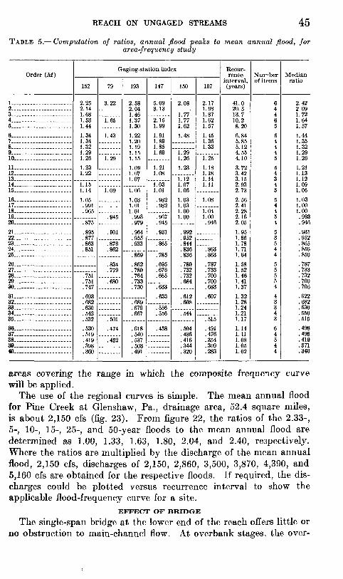
REACH ON UNGAGED STREAMS 45
TABLE 5. Computation of ratios, annual flood peaks to mean annual flood, forarea-frequency study
Order (Af )
1... __ _2...... .... ..... ....3 45..... ..............
6 .. ..... ... ...7 . 8 9 10
11 12 13 14... _ -.-- __ 15
16 17 _ ..18 19 20
21 22 23 24 25
26 27 28 29 30
31 32 33 34... .... ........35
36.. 37 38 39 40
Oaging-station index
152
2.25 2.141.681.53
1.34 1.341.321.291.26
1.22
1.151.14
.965
S7<;
.895Q77
.863
.851
.751
.751
.747
.682
.630<;49
.532
.530
.519
.419
.398
.360
79
3.22
1.65
1.43
1.29
1.09
.945
.901
.876
.862
.834
.779
.680
.501
.474"""432"
193
2.58 2.04 1.461.37 1.30
1.22 1.20 1.19 1.15 1.15
1.09 1.07 1.07
1.06
1.03 1.01
.993
.979
.964QCK
.933
.869
.862
.780
.764
.733
.730
.689
.679
.667
.618
.540
.537
.491
147
5.09 3.13
2.15 1.99
1.91 1.89 1.85 1.69
1.211.08
1.03 1.01
.982
.982
.967
.945
.931
.865
.785
.695
.676
.665
.633
.633
.556
.556
.458
150
2.08
1.77 1.77 1.62
1.48
1.29 1.26
1.23
1.121.07 1.06
1.03 1.03 1.00 1.00
.992
.844
.836
.836
.780
.732
.732
.684
.612
.608
.544
.504
.436
.416
.344
.320
197
2.17 1.98 1.87 1.62 1.57
1.45 1.36 1.33
1.25
1.18 1.18 1.14 1.11
1.08
1.04 1.00 .946
.863
.863
.787
.733
.700
.700
.683
.607
.515
.491
.476
.354
.309
.283
Recur rence
interval, (years)
41.0 20.5 13.7 10.2 8.20
6.84 5.85 5.12 4.55 4.10
3.72 3.42 3.15 2.93 2.73
2.56 2.41 2.28 2.16 2.05
1.95 1.86 1.78 1.71 1.64
1.58 1.52 1.46 1.41 1.37
1.321.28 1.24 1.21 1.17
1.14 1.11 1.08 1.05 1.02
Nunber of items
6 4 4 6 5
6 4 4 4 5
5 4 34 5
5 4 4 5 4
5 3 5 4 4
5 5 5 5 4
4 3 3 4 3
6 4 5 4 4
Median ratio
2.42 2.09 1.72 1.64 1.57
1.44 1.35 1.32 1.29 1.26
1.21 1.13 1.12 1.09 1.06
1.03 1.00 1.00 .993 .946
.931
.952
.865
.856
.850
.787
.733
.732
.700
.706
.622
.682
.630
.550
.515
.498
.498
.419
.371
.340
areas covering the range in which the composite frequency curve will be applied.
The use of the regional curves is simple. The mean annual flood for Pine Creek at Glenshaw, Pa., drainage area, 52.4 square miles, is about 2,150 cfs (fig. 23). From figure 22, the ratios of the 2.33-, 5-, 10-, 15-, 25-, and 50-year floods to the mean annual flood are determined as 1.00, 1.33, 1.63, 1.80, 2.04, and 2.40, respectively. Where the ratios are multiplied by the discharge of the mean annual flood, 2,150 cfs, discharges of 2,150, 2,860, 3,500, 3,870, 4,390, and 5,160 cfs are obtained for the respective floods. If required, the dis charges could be plotted versus recurrence interval to show the applicable flood-frequency curve for a site.
EFFECT OF BRIDGE
The single-span bridge at the lower end of the reach offers little or no obstruction to main-channel flow. At overbank stages, the over-

46 FLOOD-PLAIN PLANNING
flow area at the left end of the bridge is not obstructed by a bridg approach and permits the overflow to pass with little restrictior Were the bridge a definite channel constriction, the procedures out lined in phases I and II for similar examples would apply.
STAGHE-DISCHARGHE RELATIONS
The slope-conveyance method, as outlined in phase I, was use to develop a rating curve for section B. The irregularity of th stream bed profile precluded its use in determining flood slopes in th reach. Consequently, the average slope of the water surface betwee stations 160 and 560 (fig. 21), as determined during the field survey was used in the computations for the rating curve. Because th bridge at the downstream end of the reach cause? little or no bad water, the slope was assumed to be constant throughout the ranr: of computation. The cross section and rating curve are shown i figures 24 and 25. A more accurate estimation o* flood slopes coul be obtained from high-water marks defining the water surface through out the reach for a specific flood crest, but these data were nc available at this location.
Roughness coefficients, or n values, were chosen as follows:Part of reach General characteristics
Channel.-______________ Straight, clean, with gravel bot tom.
Left and right banks.___ Rushes and brush with sirglemedium-sized trees in line, spaced about 50 feet apart.
Grass and asphalt, little obstruc tion.
Scattered buildings, hedges ______
Roughness coefficient (i 0.03
. 0 4
Top of left bank androad.
Left overbank beyondroad.
.02
0. 040 to 0. 0£
z 52 L_l S
600 400 300 200
HORIZONTAL DISTANCE, IN FEET
100
FIGURE 24. Cross section, Pine Creek at Olenshaw, Pa. Slope-conveyance computations are shown -page 47.
FLOOD-PLAIN MAP
The method for preparing flood-plain maps has been described an illustrated on page 23. No topographic maps of suitable scale wei available for the reach nor was complete topographic detail obtaine in the field survey. In lieu of a complete flood-plain map, the est

REACH ON UNGAGED STREAMS 47
Cross section B, slope-conveyance computations
Stage (feet)
47.5
49.0
51.9
EC n
Section
... ..do .
... ..do do do . do ... ..do .....do . do . ......do. .
bank.
. do .... .
.....do........ do
bank. ... ..do..... ........do........ do
n
0.044.030.044.044.030.044.025.044.030.044.044
.025
.044
.030
.044nOK
.050
.045
.040
1.486TO
33.849.533.833.849.533.859.433.849.533.833.8
59.433.849.533.859.4
29.733.037.2
A(square feet)
987
321
141101065
2463916
69137394101107
88418980
R(feet)
0.492.21.18
1.153.86.61.69
3.566.752.371.78
5.027.49
10.856.202.97
4.403.803.42
RU*
0.621.70.32
1.102.46.72.78
2.343.571.781.47
2.933.834.903.382.07
2.682.442.27
K
1907,320
30780
17, 170240460
5,14043,4702,350
790
12, 01017,74095,56011,54013,160
7,00033,66082,760
S (feet per
foot)
0.0011.0011.0011.0011.0011.0011.0011.0011.0011.0011.0011
.0011
.0011
.0011
.0011
.0011
.0011
.0011
.0011
gi/a
0.0332.0332.0332.0332.0332.0332.0332.0332.0332.0332.0332
.0332
.0332
.0332
.0332
.0332
.0332
.0332
.0332
(cfs)
6243
126
5708
15171
1,4437826
399589
3,173383437
2321883
i 2, 171
Total
(cfe)
250
604
1,707
8,293
Q corrected for angle of flow by applying factor of 0.79 (sine 52°).
0123456
DISCHARGE, IN THOUSANDS OF CUBIC FEET PER SECOND
FIGURE K. Stage-discharge relation .Pine Creek at Qlenshaw ,Pa.
mated maximum depths of inundation for the different floods over the east-west road are shown on figure 20 to indicate the degree of flooding.

48 FLOOD-PLAIN PLANNING
If a map of the flooded areas in this reach had been required, floe profiles would have been defined for the entire reach. A definit break in the streambed and water-surface profiles is evident betweeT sections A and B (fig. 21). Under these circumstances, it probabl; would have been necessary to compute a rating curve for section ^ to define the upstream end of the profiles for the different floods Because of the apparent uniformity in slope downstream from abou station 160, the flood profiles for the lower two-thirds of the reac 1 might have been estimated by assuming that the same slope used r computing the rating curve at section B was effective.
PART 2. APPROACH BYPASSING DETERMINATION OP DISCHARGK
A quick and simple method of obtaining depth-frequency data wa sought in this part of the study. An attempt was made here t relate some feature, or features, of the channel geometry and th drainage basin to the depth of flow for floods of selected averag frequency. If this could be done, the size and frequency of overflow could be estimated from measurements of the stream channel ar drainage basin, bypassing the determination of discharge. Th objective in this part of the study was to establish, if possible, rulf of-thumb relation that might be useful in estimating the depth art frequency of flooding at the numerous locations where streamflo* records are nonexistent but which would still have to be considere in any over-all plan for areas larger than a single community.
DATA AVAILABLE
Data on the physical features of Pennsylvania streams were obtaine< by a special survey at more than 150 stream-gag:ng stations havin drainage areas ranging in size from less than 5, to more than 10,00 square miles. At each gaging station, the follovdng measurement were made at a selected cross section, called the index section: (a average channel depth for bankfull flow this was taken as th height of the low bank above the average streambed elevation; (b the stage reading at the gage for bankfull flow at the index sectior (c) channel and valley width; (d) orientation of the channel in th flood plain.
These field data were obtained with a minimunr of tools or instru ments. Only a hand level and rule were used in making these meas urements, and distances were obtained by pacing.
The index sections were chosen where the channel and flood plaii were thought to be typical of the stream in the reach near the gage The index sections were selected so as to be on a straight reach o channel, and upstream, preferably one channel width, from the con trol section for the gage. Bankfull depth at the index section wa referred to the gage datum so that the rating curve for the gage coul be adjusted for application to the index section.

REACH ON TJNGAGED STREAMS 49
FLOOD FREQUENCY
Records for the gaging stations covered by the special survey were examined for quality of the discharge data, length of record, adequacy of the data obtained in the special survey, and location with respect to flood plain. Stations at which the flood flows were materially affected by reservoir regulation were excluded. More than 100 records were selected for analysis (table 6).
For the five stations in the Youghiogheny-Kiskiminetas basin (stations 139, 141, 146-148 in table 6), the mean annual flood adjusted to the period 1884-1950 was taken from the tabular value? contained in U.S. Geological Survey Circular 204. Discharges for the 10-, 25-, and 50-year floods, also for the period 1884-1950, were computed from the curve contained in the same circular.
For stations in the Delaware River basin (those between stations 259 and 355, inclusive, in table 6), the discharge for the mean annual flood for each station was obtained from the base data used for compiling an open-file report 2 on flood frequencies in the Delaware River basin. Discharges for the 10-, 25-, and 50-year foods were then computed using the appropriate curves contained in the open- file report. A base period of 1913-55 was used for the stations in the Delaware River basin.
For the rest of the stations listed in table 6, flood discharge-fre quency data were obtained from work now in progress (April 1959) on a statewide flood-frequency report for Pennsylvania. These data are provisional and subject to revision upon final checking and review in the Washington office. The base period for these data is 1914-57. The 2.33-year, or mean annual flood,'for each station was obtained from a flood-frequency curve computed from the record for that station, expanded where necessary to encompass the period 1914-57. Discharges for floods of other frequencies were obtained by multiply ing the mean annual flood for each station by the approprate factor obtained from regional curves developed in the current statewide study.
STAGE-DISCHARGE RELATIONS
For each station, the gage heights for the selected flood discharges were taken from the most recent rating table (a tabulation of gage heights and corresponding discharge computed from the rating curve) available for the station. Some rating curves were extended logarith mically to obtain gage heights for all the discharges listed. These gage heights were converted to average depth of flow at the index section by an adjustment computed from the difference between the gage height and the average depth for bankfull flow at the index section. The computed depths, with corresponding discharges, are contained in table 6.
s Tice, Ricaard H., 1958, Delaware River basin flood frequency: U.S. Qeologioal Survey open-file report.

TA
BL
E 6
. P
enn
sylv
an
ia s
trea
m-g
agin
g s
tati
on d
ata
[Dis
char
ges
for
stat
ions
139
, 141
, 146
-148
are
for
per
iod
1884
-195
0; t
hose
for
sta
tion
s 25
9 to
355
are
for
per
iod
1913
-55;
and
tho
se f
or r
emai
nder
are
for
per
iod
1914
-57]
Or
O
Sta
tion
num
ber
and
stat
ion
2. A
llegh
eny
Riv
er a
t E
ldre
d_____________
6. A
llegh
eny
Riv
er a
t K
inzu
a_. .._
._....
12.
Bro
kens
traw
Cre
ek a
t Y
ou
ng
svil
le--
-_--
....
..16
. T
ione
sta
Cre
ek a
t L
ynch..___________
22.
Oil
Cre
ek a
t R
ouse
vill
e---
-__-
----
-._-
-___
__
24.
Fre
nch
Cre
ek a
t C
arte
rs C
orn
ers-
...-
-____
31.
Suga
r C
reek
at S
ug
arc
reek
__
__
..._
.._
_
46.
Red
bank
Cre
ek a
t St
. C
harl
es.
__...........
49.
Mah
onin
g C
reek
at
Punxsu
taw
ney
___.....
50.
Lit
tle
Mah
onin
g C
reek
at
McC
orm
ick........
57.
Cro
oked
Cre
ek a
t Id
aho_....___..._
..79
. B
uffa
lo C
reek
nea
r F
reep
ort
-__
__
----
----
--12
5. D
unka
rd C
reek
at
Sh
ann
op
in_
---.
_.-
....
...
127.
Sou
th F
ork
Ten
mile
Cre
ek a
t Je
ffer
son_.....
130.
Red
ston
e C
reek
at W
alt
ers
burg
.._..__..
139.
Cas
selm
an R
iver
at
Mark
leto
n______._
14
1. L
aure
l H
ill
Cre
ek a
t U
rsin
a..
__
__
__
__
_14
6. Y
ough
iogh
eny
Riv
er a
t C
onne
llsv
ille
____
_-14
7. G
reen
Lic
k R
un a
t G
reen
Lic
k R
eser
vo
ir_
_.
148.
You
ghio
ghen
y R
iver
at
Sute
rsvil
le.-
----
--....
152.
Cha
rtie
rs C
reek
at
Carn
eg
ie_
-__
.-.-
__
-..
186.
Lit
tle
Shen
ango
Riv
er a
t G
reen
vil
le._
__....
187.
Pym
atun
ing
Riv
er n
ear
Ora
ngev
ille
.---
--.-
- 19
3. C
onno
quen
essi
ng C
reek
at
Haz
en_
__
__
_..
..19
4. S
lippe
ry R
ock
Cre
ek a
t W
urt
emburg
__.....
197.
Rac
coon
Cre
ek a
t M
offa
tts M
ills
.-_
__
__
...
259.
Wes
t B
ranc
h L
acka
wax
en R
iver
at
Pro
mpt
on26
0. D
yber
ry C
reek
at D
yberr
y-.
....._
...
261.
Lac
kaw
axen
Riv
er n
ear
Hones
dal
e... .--
-_.-
263.
Mid
dle
Cre
ek n
ear
Haw
ley..
__
__
__
__
__
264.
Lac
kaw
axen
Riv
er a
t H
aw
ley
.__
__
_-.
__
28
0. B
ush
Kill
at S
ho
em
ak
ers
....
....
...
....
....
296.
Leh
igh
Riv
er a
t S
tod
dar
tsv
ille
.._
__
__
__
_29
7. L
ehig
h R
iver
at
Tan
ner
y.._______...........
300.
Wild
Cre
ek a
t H
atc
hery
.......................
301.
Pob
onop
o C
rcek
n^ar
Par
rvvi
lle
____
__
Region
Drai
nage
ar
ea, A
(squ
are
mile
s)
550
2,179
321
233
300
208
166
528
158 87 191
137
229
180 74 382
121
1,326 3.1
1,71
525
710
416
9356
398
178 60 63 164 78 290
117 92 332 17 109
Bank-
full
width,W
(feet) 130
393
158
170
245
115
120
200
127 80
140
110 60 79 70
131
160
323 36
590
187 60
100
188
160
130 86
102
171
121
132
108
107
228 39
lift
2.06
2.36
1.42
1.17
1.11
1.35
1.18
1.62
1.11
1.04
1.17
1.12
1.96
1.51
1.03
1.71 .87
2.02 .29
1.71
1.17
1.32
1.30
1.38
1.58
1.17 .83
.79
.98
.80
1.48
1.04 .93
1.21 .66
.97
Bed
slop
e, S
(f
eet
per
foot
)
0.00
0445
.000
858
.002
08.0
0165
.002
00.0
0200
.003
85.0
0143
.000
855
. 001
04. 0
0104
. 001
94.0
0305
.001
41.0
0494
.002
88.0
0148
.045
5.0
0027
8.0
0125
.000
996
.000
381
.000
818
.002
84.0
0130
.002
44.0
0162
.001
67.0
0197
.002
60.0
0580
.002
23. 0
0460
.014
000
974
Sl/
3
0.07
6.0
95.1
28.1
18.1
26.1
26.1
57.1
13.0
95.1
01.1
01.1
25.1
45
.112
.170
.142
.114
.357
.065
.108
.100
.072
.094
.142
.109
.135
.117
.119
.125
.137
.180
.131
.166
.241
.140
27.1
24.8
11.1
9.9
8.8
10.7 7.5
14.3
11.7
10.3
11.6
9.0
13.5
9.2
10.1 6.1
17.7 .8
226
.410
.813
.218
.114
.711
.110
.76.
26.
78.
26.
410
.85.
87.
17.
32.
76.
9
Dis
char
ge,
Q,
in t
housa
nds
of c
ub
ic f
eet
per
sec
ond,
an
d d
epth
of
wat
er,
H,
in f
eet,
for
flo
ods
of i
ndi
ca
ted f
requ
enci
es
2.33
-yea
r
Q
H
7.3
32.0 7.5
5.4
8.0
7.2
5.3
12.2
4.5
3.4
6.5
4.2
7.8
6.0
2.2
12.1 5.2
35.6 .3
40.0
5.9
2.8
3.2
8.6
8.3
5.4
3.2
4.3
6.1
3.0
9.8
2.1
2.6
2.1
14.5
10.0
9.2
8.0
7.8
9.3 6.7
11.3
8.3
8.7
12.3 7.3
9.8
10.2
6.4
8.4
5.9
14.2
2.8
16.5
8.6
9.8
10.0
10.8
7.7
7.3
6.6
7.9
7.4
8.5
12.2
3.9
4.3
6.6
3.0
4.1
10-y
ear
Q
H
11.9
52.1
12.2 8.9
13.0
11.7
8.6
19.9
7.3
5.6
10.6
6.9
12.8
9.8
3.6
20.7
8.9
60.9 .5
68.4
9.6
4.5
5.3
14.0
13.5
8.7
6.0
8.1
11.5
5.6
18.5 3.9
5.7
14.5 1.5
4.0
17.3
13.9
11.3
10.3
9.6
11.1 8.4
15.0
11.0
10.6
15.4
9.4
11.8
14.2 9.5
10.2
8.8
18.0
3.2
23.1
11.5
11.1
11.2
13.6
9.7
9.2
9.5
9.5
11.1
12.0
16.7 5.3
6.9
10.4
3.8
6.4
25-y
ear
Q
H
14.8
65.9
15.4
11.2
16.5
14.8
10.8
25.1
9.2
7.1
13.4
8.7
16.2
12.4 4.6
26.1
11.3
76.8 .6
86.4
12.2
5.7
6.6
17.7
17.1
11.0
7.9
10.7
15.3
7.4
24.5 5.2
8.5
21.9
2.0
5.3
18.6
16.3
12.8
11.6
10.3
11.9
9.4
17.2
12.6
11.7
17.
110
.713
.116
.511
.411
.210
.420
.1 3.4
27.0
13.2
12.2
11.9
14.8
10.9
10.2
11.2
10.2
13.4
14.1
19.0 6.1
8.3
13.0
4.2
7.6
50-y
ear
Q
II
17.9
78.4
18.4
13.4
19.6
17.7
12.9
29.9
10.9
8.4
15.9
10.4
19.2
14.7
5.4
30.2
13.1
89.0 .8
100 14
.56.
87.
921
.020
.313
.1 9.5
12.8
18.3
8.9
29.4 6.2
11.1
28.4
2.4
6.4
19.7
18.6
14.1
12.8
10.9
12.3
10.2
18.2
14.0
12.4
18.4
11.8
14.2
18.4
13.0
11.8
11.7
21.7
3.7
29.5
14.5
13.2
12.5
15.7
11.9
11.1
12.6
10.7
15.1
15.8
20.5 6.6
9.4
14.9
4.5
8.7

303.
Leh
igh
Riv
er a
t W
aln
utp
ort
___ _
_________.
304.
Lit
tle
Leh
igh
Cre
ek n
ear
All
ento
wn
__
_..._
__
__
_30
5. J
orda
n C
reek
at A
llen
tow
n_
__
_-.
.-.-
.-..
.._
__
.30
7. L
ehig
h R
iver
at
Bet
hle
hem
... _
___________.
320.
Toh
icko
n C
reek
nea
r P
ipersvil
le .
332.
Nes
ham
iny
Cre
ek n
ear
Langhorn
e.-
-.________.
340.
Lit
tle
Sch
uylk
ill
Riv
er a
t T
am
aqua....._
___......
345.
Sch
uylk
ill
Riv
er a
t P
ott
stow
n._
____________
347.
Per
kiom
en C
reek
at
Gra
terf
ord
-__._
__._
_____.
350.
Sch
uylk
ill
Riv
er a
t P
hil
ad
elp
hia
....
....
....
__
__
.35
5. C
hest
er C
reek
nea
r C
heste
r...
.-_
__
__
__
__
__
464.
Sus
queh
anna
Riv
er a
t T
ow
anda._
....._
.__.
465.
Tow
anda
Cre
ek n
ear M
onro
eto
n..._
....__..__.
468.
No
rth
For
k M
ehoo
pany
Cre
ek n
ear
Lo
velt
on
..._
..46
9.
Tun
khan
nock
Cre
ek a
t D
ixon___________....
470.
Lac
kaw
anna
Riv
er a
t A
rchbold
..__________.
473.
Lac
kaw
anna
Riv
er a
t O
ld F
org
e..__________..
475.
Tob
y C
reek
at L
uzern
e .
- -
476.
Sol
omon
Cre
ek a
t W
ilkes-
Barr
e..__________.
477.
Wap
wal
lope
n C
reek
nea
r W
apw
allo
pen.
__
__
__
.47
9. F
ishi
ng C
reek
nea
r B
loom
sburg
..._
_________.
480.
Lit
tle
Fis
hing
Cre
ek a
t E
yers
Gro
ve..._
__
__
__
.48
2. S
usqu
ehan
na R
iver
at
Danvil
le..._
__________
483.
Wes
t B
ranc
h S
usqu
ehan
na R
iver
at
Bow
er..-
........
484.
C
lear
fiel
d C
reek
at
Dim
elin
g____ _
_..._
________
485.
M
osha
nnon
Cre
ek a
t O
sceo
la M
ills
__
__
_..
....
.48
7. D
rift
woo
d B
ranc
h S
inne
mah
onin
g C
reek
at
Ste
rlin
g R
un______--
____....____..._
...... _
_._
_.
488.
Sin
nem
ahon
ing
Cre
ek a
t S
innem
ahonin
g____....
490.
K
ettl
e C
reek
at
Cro
ss F
ork...._....._
....._
....
494.
S
prin
g C
reek
nea
r A
xem
an
n_
__
_..
__
__
__
__
. 49
7. N
orth
Bal
d E
agle
Cre
ek a
t B
eech
Cre
ek S
tati
on......
500.
Blo
ckho
use
Cre
ek n
ear
Eng
lish
Cen
ter_
__
__
_....
501.
L
ycom
ing
Cre
ek n
ear
Tro
ut R
un__________..
505.
Loy
also
ck C
reek
at L
oyals
ock..______ .......
506.
Mun
cy C
reek
nea
r S
onest
ow
n___________...
508.
Wes
t B
ranc
h S
usqu
ehan
na R
iver
at
Lew
isb
urg
......
510.
Sha
mok
in C
reek
at
Wei
gh S
cale
--__________.
511.
Per
m C
reek
at
Pen
ns C
reek
.._
__
__
__
__
__
.51
2. E
ast
Mah
anta
ngo
Cre
ek n
ear D
alm
ati
a.. ......
513.
Fra
nkst
own
Bra
nch
Junia
ta R
iver
at
Wil
liam
sbur
g..
516.
Sou
th B
ald
Eag
le C
reek
at
Tyro
ne__________.
517.
Lit
tle
Juni
ata
Riv
er a
t S
pruc
e C
reek_..
__ .
....
519.
Ju
nia
ta R
iver
nea
r H
unti
ngdon,.__-.
-.-.
.___...
520.
Sta
ndin
g S
tone
Cre
ek a
t H
unti
ngdon....._
_____
521.
Dun
ning
Cre
ek a
t B
eld
en
...._
.__
__
__
__
_.
523.
Bru
sh C
reek
at G
ap
svil
le_
__
__
_.._
__
__
__
-52
5. R
ayst
own
Bra
nch
Jun
iata
Riv
er a
t S
ax
ton
__
__
_.
526.
G
reat
Tro
ugh
Cre
ek n
ear
Mark
lesb
urg
_______.
527.
Ray
stow
n B
ranc
h Ju
nia
ta R
iver
nea
r H
unti
ngdon...
528.
Ju
nia
ta R
iver
at
Map
leto
n D
epot.
__________.
1 App
roxi
mat
ely
(by
com
puta
tion
).
889 81 76
1,279 97 210 43
1.147
279
1,89
3 617,
797
215 35.2
383
108
332 32 16 44 274 57
11,220 315
371 69 272
685
136 87 559 38 173
443 24
6,84
7 54 301
162
291 44 220
816
128
172 37 756 85 957
2,030
450 78 104
!330 105
160 66
'330 190 73
'900 170 50 192
116
200 41 73 65 166 88
1 1,
350 180
188 57 229
314
145
128
180 60 115
500 54
'950 60 240
130
180 65 90 265
125 85 38 275 88 255
217
1.41
1.02 .85
1.97 .96
1.14 .81
1.87
1.21 .91
2.94
1.13 .84
1.41 .96
1.29 .88
.47
.82
1.28 .80
2.88
1.32
1.40
1.10
1.09
1.48 .97
.82
1.76 .80
1.22 .94
.67
2.68 .95
1.12
1.12
K27
.82
1.56
1.76
1.01
1.42 .99
1.66 .98
1.94
3.06
. 001
31. 00175
. 00157
. 000
948
. 00173
. 000
930
. 00768
. 000421
. 001
05
. 00202
. 000
628
. 00262
.008
30. 00173
. 004
55. 004
44.0
122
. 00350
. 00576
.00207
. 00323
. 000201
. 00156
. 00137
. 00185
.002
22. 00152
.00285
. 00412
. 000795
. 00750
. 00229
. 00247
.010
2.000322
.00900
.00156
. 00159
. 00168
.005
30.00274
. 00154
. 00100
.000
880
.00342
. 000
993
.011
7. 000
848
.001
11
.109
.120
.116
.098
.120
.098
.198
.075
.102
.126
.086
.138
.202
.120
.166
.164
.230
.152
.179
.127
.148
.058
.116
.111
.123
.130
.115
.142
.160
.093
.196
.132
.135
.217
.068
.208
.116
.117
.119
.174
.140
.115
.100
.096
.151
.100
.227
.095
.104
12.9 8.5
7.3
20.1 8.0
11.6 4.1
24.9
11.9 7.2
342
8.2
4.2
11.7 5.8
7.9
3.8
3.1
4.6
10.1 5.4
49.7
1L4
12-6 9.0
8.4
12.9 6.8
5.1
18.9 4.1
9. 2 7!o
3.1
39.4 4.6
9.6
9.6
10.7 4.7
11.1
15.3
10.1
14.8 6.5
16.6 4.3
20.4
29.4
21.9 .8 2.4
24.5 6.5
9.7
1.8
22.0
16.4
47.8 3.2
119 10.4 1.8
16.1 3.1
8.0
1.2
1.0
1.4
10.2 2.1
137 8.
38.
61.
8
8.8
16.6 3.2 .7
10.9 2.3
6.9
18.3 1.4
115 1.
47.2
5.0
7.8
1.7
5.7
16.3 2.8
4.5
1.0
15.1 2.0
15.3
29.5
6.5
4.0
5.4
10.0 7.8
9.6
4.0
12.1
11.1
11.3 8.4
17.4 9.3
3.4
9.1
4.1
7.1
3.3
4.9
5.1
7.4
4.7
20.4 8.6
8.4
5.7
6.3
8.5
5.3
3.1
9.6
5.1
9.1
5.6
4.0
19.0 3-4
8.3
8.5
11.5 3.7
8.1
11.5 7.2
8.9
6.9
11.8 5.7
12.1
16.2
47.1 1.6
4.6
52.7
12.2
18.4 3.4
35.4
31.0
77.0 6.0
194 17.0 2.9
26.2 5.0
13.0 2.0
1.7
2.3
16.6 3-4
223 13.5
14.0 2.9
14.3
27.1 5.1
1.1
17.5 3.8
11.2
29.8 2.2
185 2.
211
.6 8.0
12.6 2.7
9.2
26.2 4.5
7.2
1.6
24.3 3-2
24.6
47.5
11.0 5.7
6.4
16.3
10.3
13.5 5.8
16.1
15.3
13.5
11.0
24.3
11.1 4.1
11.5 5.6
10.0 4.1
6.6
6.7
9.6
6.3
28.2
10.8
10.5 8.2
8.1
11.7 6.8
3.8
12.3 6.4
12.0 7-0
4.8
24.7 4.2
10.8
11.2
13.1 4.6
10.1
14.5 8.7
10.9 7.9
14.7 6.8
15.8
20.7
71.0-
2.1
6.0
79.4
16.2
24.3 4.5
43.8
41.0
95.2 7.9
245 21.4 3.6
33.2 6.4
16.5 2.6
2.1
2.9
21.0 4.3
282 17.1
17.7 3.7
18.1
34.2 6.5
1.4
21.2 4.7
14.2
37.9 2.8
224 2.6
14.0 9.8
15.2 3.3
11.1
31.8 5.5
8.8
1.9
29.4 3.9
29.8
57.5
14.7 6.6
6.9
21.3
11.6
15.6 6.8
18.4
17.4
14.6
12.4
28.8
12.0 4.5
12.8 6.5
11.9 4.5
7.6
7.7
10.9 7.3
33.0
12.0
11.9 9.9
9.1
13.7 7.6
4.2
13.6 7.1
14.0 7.8
5.1
27.3 4.7
11.8
12.4
13.8 5.1
11.0
15.7 9.3
11.8 8.3
16.0 7.3
17.4
28.2
92.3 2.5
7.2
103 19.4
29.2 5.3
50.6
49.2
110 9.
529
2 25.5 4.3
39.4 7.6
19.6 3.1
2.5
3.4
25.0 5.1
336 20..
321
.1 4.4
21.6
40.7 7.7
1.6
24.1 5.6
16.9
44.8 3.3
254 3.0
15.9
11.1
17.2 3.7
12.6
36.0 6.2
9.9
2.2
33.4 4.4
33.8
65.2
16.5 7.2
7.2
24.7
12.7
17.2 7.6
20.2
19.0
15.6
13.6
32.5
12.8 4.8
13.8 7.4
13.6 4.9
8.5
8-4
12.0 8.1
37.1
13-1
13.0
11.5 9.9
15.4 8.3
4.4
14.6 7.7
15.6 8.3
5.4
29.1 5.1
12.6
13.3
14.4 5.5
11.6
16.5 9.8
12.5 8.6
16.9 7.7
18.4
24.4

TABL
E 6
. P
enns
ylva
nia
stre
am-g
agin
g st
atio
n da
ta C
on
tin
ued
[Dis
char
ges
for
stat
ions
139
,141
,146
-148
are
for
per
iod
1884
-196
0; t
hose
for
sta
tion
s 25
9 to
355
are
for
per
iod
1913
-55;
and
tho
se f
or r
emai
nder
are
for
per
iod
1914
-57]
to
Stat
ion
num
ber
and
stat
ion
Reg
ion 1 1 1 1 1 2 1 1 2 2 2 2 2
Dra
inag
e ar
ea, A
(s
quar
e m
iles)
205
164
214 57
200
470
333 14
51
0 74
117
222
324
Ban
k-
full
wid
th,
W(f
eet) 135
110
175
120
160
165
140 40
225 78
68
11
8 14
1
JAI
W
1.23
1.
22
1.11
.6
9 1.
12
1.69
1.
54
.59
1.51
.9
7 1.
31
1.37
1.
52
Bed
sl
ope,
S
(fee
t pe
r fo
ot)
0.00
105
. 005
22
. 001
00
.002
32
. 001
44
. 000
388
. 000
762
.006
50
. 001
33
. 001
46
.002
00
. 000
592
Si/
'
0.10
2 .1
73
.100
.1
32
.113
.0
73
.091
.1
87
.110
.1
14
.126
.0
84
SA/
WS
l/3
12.0
7.0
11
.1
5.2
9.
9 23
.1
17.0
3.2
8.8
11
.5
10.9
18
.1
Dis
char
ge,
Q, i
n th
ousa
nds
of c
ubic
feet
per
sec
ond,
an
d de
pth
of w
ater
, H
, in
fee
t, fo
r flo
ods
of in
di
cate
d fr
eque
ncie
s
2.33
-yea
r
0 7.6
2.8
6.8
3.4
8.8
8.4
9.8 .6
16.2
2.
5 2.
5 4.
4 7.
2
H 9.9
3. 6
9.
0 6.
4 8.
1 8.
8 10
.3
4.5
13.0
6.8
6.
6 7.
3 7.
3
10-y
ear
0
12.2
4.
6 11
.2
5.4
14.2
13
.5
16.0
1.
0 26
.1
4.1
4.0
7.1
11.5
H 12.3
5.
2 12
.0
7.9
10.3
11
.1
13.6
5.
5 16
.7
7.6
8.4
9.5
9.8
25-y
ear
P
14.8
5.
6 14
.1
6.5
17.2
16
.4
21.2
1.
2 31
.6
4.9
4.8
8.6
13.9
H 13.6
6.
0 13
.7
8.7
11.3
12
.1
15.3
5.
9 18
.5
8.0
9.1
10.5
11
.0
50-y
ear
P
16.8
6.
3 15
.1
7.4
19.4
18
.6
21.6
1.
4 35
.8
5.6
5.5
9.7
15.8
H 14.4
6.
6 *H
14
.3
tf
9.3
O
12.0
O
12
.8
y
15.9
M
6.
2 fi
19
.8
>8.3
a
9.6
^
11.2
11.9
|g

REACH ON UNGAGED STREAMS 53
CORRELATION OF FLOOD DEPTHS WITH PHYSICAL FEATTIRES OF DRAINAGE AREA AND CHANNEL
Natural forces create stream channels that are in balance with the magnitude and frequency of the flows that they are called to carry. For mature streams that are in a state of quasi-equilibrium, there may be a correlation between some measurable feature, or features, of the river channel and basin and the height and frecuency of overflows.
Many different correlations were tried in an attempt to find a workable relation between depth, frequency, and variour physical measures of channel geometry. Early attempts were concentrated on one of the more promising of these, the relation involving average depth for bankfull flow and the stage and frequency of other floods. However, the resulting relations were not well defined. Perhaps the principal reason for the poor correlation was the difficulty in defining, identifying, and measuring the depth of bankfull flow.
The approach involving depth of bankfull flow was abandoned and a parameter that could be more easily identified and measured was sought. The width of the channel seemed to best fit these require ments and a relation was developed that showed a fair degree of consistency among the data. The final curves involved a plot of the depth of flow for a specified frequency of flood versus the quantity,
> where A is the drainage area in square miles; W is the channel
width, in feet; in most places the single-section width between the top of the left and right banks, and S is the slope of the streambed in the gage vicinity, determined from topographic maps, in feet per foot.
The expression, ~1/3 > is an approximation derived by combining the
Manning formula for open-channel flow with an equation relating flood discharge for a specific recurrence interval with drainage area. Where discharges for the 2.33-, 10-, and 50-year floods were plotted versus drainage area, it was found that the curves of relation had a constant slope of approximately 0.8. Only the intercept on the dis charge axis changed for the three floods, giving an equation of the general form, Q=CA°-*, where Q is the flood discharge in c^s, C is the intercept on the discharge axis, and A is the drainage area in square miles. By substituting this equation for the discharge term in the Manning formula, assuming that the cross-sectional area of the channel is equal to average depth times channel width and that the hydraulic radius is equal to average depth, and rounding off exponents, the depth

54 FLOOD-PLAIN PLANNING
of flow for a specific recurrence interval is estimated as equal t
01/3 * The value of C varies, depending on the size of the floe
considered (in terms of recurrence interval). But, 01/3 is a p>
rameter that can be used to relate depths of flow for floods of variov frequencies.
The definition of the slope term merits some explanation. Tr map slopes were computed from distances measured between poin where contour lines crossed the stream in the gage vicinity. Thr£ values of computed map slopes were tried in the correlations th^ computed from the 1 contour interval embracing the gage, that coir puted from 2 contour intervals with the gage located in the dowr stream contour interval, and that computed from 3 contour interval with the gage located in the middle contour interval. These pro cedures could not be followed at every gaging station listed in table because of the proximity of a dam or the mouth of the stream c because of some other abnormal condition. However, the slope use should represent the average streambed slope in the gage reach. Th best results were obtained with the slope determined from 3 cor tour intervals and this is the slope recorded in table 6, except fc stations were deviation from the regular procedure was necessary Apparently the use of the larger fall lessens the distorting effect c irregularities present in, for example, a 1-contour interval.
The depth of flow for the mean annual flood was plotted agains \IAIW
the quantity -01/3 > in figure 26. The depth for the mean annuf
flood was used in this plot because the discharge for that flood the most reliable of the several discharges computed for differer recurrence intervals for each station. Where the deviation from th curve of figure 26 was computed for each station and spotted on map, subdivision of the State into the two regions shown on plate was suggested.
Regional curves showing the relation between depth of flow fc
floods of selected frequency and the parameter, o//3 > are containe
in figures 27-30. These curves were fitted visually giving less weigl: to the few points that were widely scattered. Mathematical curv fitting was not warranted for these data.
APPLICATION OF THE SIMPLIFIED METHOD
The curves discussed in the preceding section afford a simple mear of estimating depths for the 2.33-, 10-, 25-, and 50-year floods at siti for which no hydrologic data are available. The only field measure

REACH ON UNGAGED STREAMS 55
Q 20 Oo
I I_____I_____I III5 ___ 10 20 30 40 50
1//TZ7
FIOTJRE 26. Relation of depth for mean annual flood and _1/3 , Pennsylvania streams.
ment necessary is the channel width at a representative cross section of the stream. The slope of the streambed can be determined from topographic maps, river-survey profiles, or by direct measurement in the field. The drainage area can be measured from the best maps that are available for a particular basin. After these three parameters are evaluated, the estimated depth of flow is determined from the curves applicable to the particular region.
As an example, section B on Pine Creek at Glenshaw, Pa. has a drainage area of 52.4 square miles, a channel width of 90 fe?t, a slope of 0.0011 feet per foot, and an average elevation of the streambed of
45.0 feet, assumed datum (fig. 24). From these data the factor '/3
is computed as 7.4. Entering the curves of figures 27-30 (region 1) with this value of the abscissa, depths of 7.1, 8.8, 10.0, and 10.9 feet are obtained for the 2.33-, 10-, 25-, and 50-year floods, respectively. Adding these depths to the elevation of the streambed gives water- surface elevations of 52.1, 53.8, 55.0, and 55.9 feet, respectively. These check the elevations computed in part 1, phase III, within 1.2 feet (table 7).
Table 7 also contains a comparison of the results obtained by the simplified indirect method and the more rigorous methods cf phases I and II for cross sections on Chartiers Creek in the Carnegie and May-

56 FLOOD-PLAIN PLANNING
20
10
Region 1
I500.5
20
10
10 20
20.5
Region 2
I5010 20
FIGURE 27. Kelation of depth for mean annual flood and * b:' regions, Pennsylvania.
view reaches. Comparisons for cross sections upstream from t bridge to the athletic field in the Mayview reach were not releva because of the complexities caused by the ponding effect from t debris accumulations at this bridge. Except for the Third Stre section in Carnegie and cross section E in the Mayview reach, t comparison is fairly good. The effect of bridges may explain, least in part, the comparatively poor agreement at Third Stre' No reason can be given for the poor comparison indicated for secti E in the Mayview reach except that perhaps the cross section chos may not represent this reach of stream.

TAB
LE 7
. C
ompa
riso
n of
re
sults
ob
tain
ed b
y si
mpl
ifie
d in
dire
ct m
etho
d an
d th
e m
etho
ds
of
phas
es I
and
II f
or
sele
cted
cro
ssse
ctio
ns o
n C
hart
iers
Cre
ek a
nd P
ine
Cre
ek,
All
eghe
ny C
ount
y, P
a.
Rec
urre
nce
inte
rval
, in
ye
ars
2.33
10
25
50
Ele
vati
on o
f wat
er s
urfa
ce,
in f
eet
Thi
rd S
tree
t C
arne
gie
^4=2
57 s
q m
i, W
=l4
0ft,
S
= 0.
001 2
5 (m
ap)
Str
eam
bed=
759.
0ft
Indi
rect
m
etho
d
768.
6 77
1.4
773.
2 77
4.4
From
pro
fil
e (p
i. 3)
769.
6 77
3.3
774.
9 77
6.7
Wal
nut
Stre
et
Car
negi
e ^4
=257
sq
mi,
W=1
30 f
t, 5=
0.00
125
(map
) St
ream
bed=
753.
7 ft
Indi
rect
m
etho
d
763.
6 76
6.5
768.
4 76
9.6
From
pro
fil
e (p
i. 3)
764.
7 76
7.5
769.
4 77
0.9
Sect
ion
E
May
view
,4
=157
sq
mi,
1F=1
00 f
t, 5=
0.00
141
(map
) St
ream
bed=
834.
8 ft
Indi
rect
m
etho
d
843.
8 84
6.3
848.
0 84
9.1
Fro
m p
ro
file
(pi.
3)
842.
7 84
4.3
845.
0 '8
45.7
Sect
ion
Q
May
view
,4
=157
sq
mi,
W=
ll5
ft,
S=0.
0014
1 (m
ap)
Str
eam
bed=
830.
8 ft
Indi
rect
m
etho
d
839.
4 84
1.8
843.
4 84
4.4
Fro
m p
ro
file
(pi.
3)
838.
6 84
1.0
842.
0 84
2.8
Sect
ion
/ M
ayvi
ew
^4=1
57 s
q m
i, W
=76
ft,
S=0.
0014
1 (m
ap)
Str
eam
bed=
825.
6 ft
Indi
rect
m
etho
d
835.
3 83
8.2
839.
9 84
1.3
From
pro
fil
e (p
i. 3)
835.
7 83
8.2
839.
6 18
40.9
Sect
ion
B
Qle
nsha
w
,4=
52.4
sq
mi,
W=9
0 ft
. 5=
0.00
11 (
fig.
24)
Str
eam
bed=
45.0
ft
Indi
rect
m
etho
d
52.1
53
.8
55.0
55
.9
Fro
m p
hase
II
I, p
art
1, fig
. 20
52.5
53
.8
54.3
54.7
Fro
m r
atin
g cu
rve.

5830
Oo o^ 20
10
FLOOD-PLAIN PLANNING
Region 1
20.5 10 20 50
30
20
10
5
4
3
0.5
Region 2
10
Sr,
FIGURE 28. Kelation of depth for 10-year flood and
20 50
by regions, Pennsylvania.
DISCUSSION OF RESULTS
The standard error of estimate is used as a measure of the scatte of points defining a relation curve. It is defined as the deviation or each side of the curve of relation that envelops two- thirds of the point defining the relation. That is, the chances are 2 out of 3 that for *
given value of ^/ , the observed depth of flo^T will plot withii
± 1 standard error of the curves on figures 29-32. For example, thi standard error of estimate of the curve for region 1 in figure 27 i. approximately 0.08 log unit, equivalent to about 20 percent. Thus

REACH ON UNGAGED STREAMS 59
40 Q
8 30
20
Region 1
0.5
30
10
Region 2
-\FIGURE 29. Relation of depth for 25-year flood and by regions, Pennsylvania.
O1 ' 1*
the odds are 2 to 1 that the depth of flow for the mean annual flood in region 1 as determined from the curve of figure 27 will be within about 20 percent of the actual depth for that flood.
The approximate standard error of estimate for the curves of figures 27-30 varies from slightly less than 0.08 to almcst 0.10 log unit. These values are equivalent to about 20 and 26 percent. On an average, determination of depth of flow from these curves would be within 20 to 25 percent of the correct depth for 2 out of every 3 determinations made.
582753 O 61 5

60 FLOOD-PLAIN PLANNING
Region 1
40
30
20
£ 10
Region 2
FIGURE 30. Relation of depth for 50-year flood and A /3 by regions, Pennsylvania.
Many factors influence the correlation of the data, particularly the degree to which the cross section is typical of the reach. Gagin stations are often deliberately located at typical sections wher definite and stable stage-discharge relations are likely to obtain An effort was made to reduce the errors from this source when selectin the gaging stations for analysis but all bias in the data was not re moved. The selection of an average cross section in the field depend largely on personal judgment.

REACH ON UNGAGED STREAMS 61
The quality of the topographic maps affects the accuracy of the slope term. Many of the slopes used in this study were measured from old maps that are probably less accurate than more modern maps. Perhaps the common topographic map is not the best basis for estimating the slope factor; this might deserve separate study.
The constant average value of channel roughness which is inherent in each of the carves of figures 26-30 is an approximatior. Channel roughness varies widely, especially for stages greater than bankfull, and for small streams. Different slopes and widths at different discharges further limit accuracy by causing steepening or flattening of the rating curves.
All of the above factors, and perhaps many others, affect the accuracy of the simplified indirect method and illustrate the diffi culty of achieving good correlation with relatively scant data. In terms of discharge, a 20 percent error in the depth of flow could mean the difference between a 10-year and a 50-year flood. Rule- of-thumb methods, using very little hydraulic and hydrologic data, can never give precise results. Where precision is required, detailed surveys and analyses must be made.
The method proposed here is entirely empirical and applicable only to Pennsylvania. For other areas, similar studies must be made to define the applicable relations. The regional divisions suggested for Pennsylvania are based solely on the plotting of the data. Perhaps there are physical or meteorological reasons for the regionalization shown but these were not apparent from available data; yet the differences between the regional curves seem to be significant. Be cause 100 gaging stations do not provide intensive coverage for a State as large as Pennsylvania, the regions shown on plate 4 are not accurately defined nor are they to be considered inflexible. Additional data, and refinements in their analysis, may define differer t regions in Pennsylvania in the future.
Because very little data on large streams were available, the method described here is applicable only to the smaller streams in Pennsyl vania. Only three gaging stations with drainage areas greater than 5,000 square miles were included in this analysis. However, in any general flood-zoning program, the need for a reconnaissance method is much greater on the small streams, which greatly outnumber the large ones and frequently are ungaged. Because of their economic importance, large streams are usually gaged at one or more locations so that the methods of phases I and II would be applicable.
For the engineer, the results obtained by the simplified method are perhaps more qualitative than quantitative, but ar^ useful for reconnaissance purposes and in the preliminary phases of studies having the depth of flow as a pertinent factor. The simplified

62 FLOOD-PLAIN PLANNING
approach supplies a rapid and economical method for use in pre liminary flood-plain zoning studies. It helps to provide, at minimum cost, answers to such questions as:1. Is flood-plain zoning required?2. Approximately what areas are inundated by floods of specific
frequency?3. How many zones are required?
Until the method can be refined and more generally verified, it should be confined to preliminary flood-zoning studies. The fin a establishment of zones should be based on the more rigorous proce dures outlined in other sections of this report.
FLOOD HAZARDS
The effects of floods and the hazards involved ar-? generally known However, a brief discussion of those flood hazards and conditions pertinent to flood-plain zoning or planning is desirable.
A stream in flood has two ways of damaging whatever lies in ite path or comes under its influence. The first is by the inundatior caused when the stream overflows its banks and floods large areas Inundation causes extensive damage from water and silt and is oftei a serious menace to health. Secondly, damage by high velocity often associated with floods, occurs when the stream sweeps down it'. channel and flood plain.
The overflow of a stream in flood is due to the stream being swollei beyond the capacity of its channel to carry all of its flow. This incapacity is usually aggravated, often seriously, by development; restricting the stream channel and encroaching ci the flood plain Similarly, restrictions, such as bridges or ice and debris jams, maj back water up into tributary streams and sloughs causing unexpected inundation of the adjacent areas.
The Main Street Bridge in Carnegie is an example of a hazard causec by insufficient waterway area under a bridge. Corrective measure! could reduce appreciably the height of the larger floods in the am immediately upstream from the bridge.
Aside from the scour and backwater effect caused by bridges o inadequate waterway opening, another hazard may arise from bridge, having a number of short spans with a corresponding number of pier that may cause an accumulation of debris. The brdge to the athleti field at Mayview is an example of this type of hazard.
Proper design of all bridges to reduce flood hazards is an importan phase of flood-plain planning. If all bridges were designed to spa, the entire valley, hazards from this source would be practically eliminated. However, such practice is seldom economically feasibl or necessary. The use of approach embankments extending across

FLOOD HAZARDS 63
large part of the flood plain is justified as long as proper allowance is made for the resulting backwater, and if the waterway opening is designed to permit passage of the hydraulic traffic safely without causing excessive scour.
Hazards may be produced by buildings, piers, spits of made land, or jetties deflecting the normal currents against a formerly safe and unprotected opposite bank. Although such structures may be pro tected in themselves, they may cause serious damage to the opposite bank along with detrimental changes in the stream channel for some distance downstream. Other flood hazards, not evident in an indi vidual reach, may be produced by causes outside the reach itself, such as the sudden release of water from upstream ice and debris jams, or by failure of an upstream impounding structure.
Recognition of the hazards of flood-plain occupancy does not entail complete abandonment of the flood plains; serious economic loss would result from such practice. It does imply that flood-plain usage over a period of time can be restricted to improvements and developments that are compatible with the river's inherent need for increased water way capacity during times of flood.
There are many flood-plain uses that do not unduly restrict the passage of overflows. Many communities already are converting flood-plain lands to parks, golf courses, other recreational uses, and to parking lots. Certain kinds of factories and commercial establish ments can justifiably locate on the flood plain if they are e,ware of the risk involved. The rehabilitation of Pittsburgh's "Golden Triangle" is an excellent example of a flood plain converted to usage compatible with degree of flood risk. However, the construction of homes, schools, and hospitals on exposed parts of the flood plain where loss can be catastrophic must be discouraged.
The establishment of flood zones will have little effect on the developments already on the flood plain except, perhaps, to make the present occupants more flood conscious. It can, howeA7 er, restrict new development and construction so that, over the years, the desired modification of uses is effected.
EFFECTS OF URBANIZATION
Urbanized areas, with their large proportion of impervious catch ment, intensify runoff. The effects, beyond producing local floods, generally will depend on the relative size of drainage areas and the location of urbanized areas in the watershed.
The multiple-unit housing development, with its usual shopping center, becomes an area covered with buildings, roads, and other impervious surfaces. The ground that formerly absorbed large amounts of rainfall is covered by impervious materials that intensify the rate

64 FLOOD-PLAIN PLANNING
and volume of runoff and shorten the time to peak. The runoff is generally collected into a storm-sewer system. When the storm-sewer capacity becomes overtaxed during heavy rain storms, ponding in streets or overflow into basements results.
Where the urban development covers a small part of the total drain age area, its effects are primarily local. If the development is isolated or if it is confined to one of two smaller tributaries, tl e large proportion of impervious watershed area will expedite generation of the local flood peak. These floodwaters are usually passed downstream before arrival of the slower tributary flood or flood from the natural watershed upstream and thus may tend to reduce the main flood peak. On the other hand, where development is extensive on tvo or more of the tributaries and the concentrated flow from these tributaries arrives at about the same time, flood conditions will be aggravated. A concen trated inflow from a built-up area entering at the upper reaches of a steep tributary could make conditions worse by dangerously augment ing the stream velocity.
Little quantitative information is available on which to base much more than the preceding qualitative discussion. Situations are known where competent observations by responsible local resident? show more frequent occurrence of ordinary floodir,^ in recent years. This observation may be valid over a period of years for a small stream where the proportion of impervious catchment has progres sively increased through urban development, anc1 such impervious area has become an appreciable part of the stream drainage basin. On the other hand, the floods may seem larger and more frequent because the damage possibilities have been increased and damage occurs more frequently. This may happen even though the actua" flood magnitude has not increased. To provide valid, direct com parison, data on the flood regimen should be obtained prior to, as well as after, extensive urban development. Collection of basic hydrologic data should start as soon as possible. Where a community is already established, intensive study of the area may develop some relief measures.
Because of recent extensive development of closely built up com munities, and the interest shown by those engaged in community development, intensive hydrologic studies of certain areas would be justified.
ZONING CONSIDERATIONS
The purpose and scope of this study are to present methods whereby hydraulic and hydrologic data may be used for flood-plain zoning Determination of the need for zoning and the acturl establishment ol flood zones, as such, are beyond the scope of the study, and are up tc

ZONING CONSIDERATIONS 65
the discretion of the planner. However, a few points that the planner should consider are worth mentioning here.
In connection with the appraisal and information phases of flood- plain planning, conspicuous markers or monuments should be placed defining the flood zones or indicating the stages reached by notable floods in an area, thus increasing public awareness to floods. Flood zones should be related to stages at a gaging station whe^e possible. If feasible, a suitable outside gage, accessible and visible to the public, should be installed. Even if flood-plain zoning is not immediately accomplished, the community can distribute flood maps to interested or affected individuals and to such groups as loan agencies and bankers. Work involving flood-plain planning, now limited to individual or isolated areas, should develop into a regional effort to coordinate the work and to promote uniform standards.
The user of this study must determine the number of flood zones to be set in his particular area. The answer to this problem depends on the physical characteristics of the area to be zoned and the purpose of, and need for, zoning. In the present study, flood lines for selected recurrence intervals have been computed and shown on the profiles and maps. These lines are for guidance only, and are not intended to delineate the final number of necessary zones.
The determination of zones for floods exceeding 30- to 50-year recurrence intervals may be unnecessary for some aree,s. Rating curves are often very flat at the highest stages; consequently, the difference in stage between a 50- and a 100-year flood, is frequently small (about 1 foot for Chartiers Creek at Carnegie). Such ratings are typical of U-shaped valleys where the moderately rare floods inundate most of the valley floor. In the rarer floods, tl e depth of inundation and the velocity of flow are increased, but the area flooded is not materially enlarged.
In many U-shaped valleys, one flood zone may suffice. A good example is the Mayview reach of Chartiers Creek where the mean annual flood (recurrence interval of 2.33 years) inundates p, large part of the valley floor. On the other hand, the valley floor in Carnegie is not as uniform in elevation arid one flood zone may not be adequate. The Carnegie map indicates a large increase in flooded area between the 5- and 10-year floods. A possible way to resolve the question "How many zones?" is to plot a curve of flood severity in terms of recurrence interval versus area flooded. Sharp breaks in this curve could be used to define zone limits. In V-shaped valleys, typical of many smaller streams, more than one flood zone probablv would be necessary.
The future needs of the area to be zoned must also be considered. An area to be zoned primarily for agriculture and light industry would

66 FLOOD-PLAIN PLANNING
require fewer zones than one to be zoned for urban development. The planner must bear in mind his primary objective when deter mining the number of zones. From the standpoint of economics and enforcement, the least number possible is desired.
Experience with flood-plain zoning in selected areas of the United States has been described in books by Leopold and Maddock, 3 and by Hoyt and Langbein.4
CONCLUSIONS
The major flood damages occur in the flood plain areas. These damages are increased through encroachment on the flood plains and by channel restrictions. Whereas the more conventional flood- control measures reduce damage after development, flood-plain planning and zoning offer a positive approach directed toward the modification of flood-plain usage so that the damage potential is reduced or eliminated.
Appraisal of the flood hazards and determination of flood risks involved are necessary in any flood-plain zoning study. Such an appraisal can be made by application of available hydraulic and hydro- logic data concerning the streams. Analvsis of these data requires consideration of, (a) flood magnitudes, (b) their eroected frequency, and (c) the elevations reached and areas covered by the floodwaters. The product is a map that shows the areas inundatei by several floods identified by expected average frequency.
This study has been undertaken in three phases based on the hydraulic and hydrologic data available. Phase I offers a procedure using actual streamflow records for a period of years and permits an accurate appraisal of the flood potential of the reach of stream in volved. Accuracy is increased with the length of record, the amount of detail obtained in the surveys, and the reliability of pertinent data. The methods outlined in this phase should be used for final zoning in any area near a long-term gaging station.
Phase II can be used where the area being zoned is on a gaged stream, but distant from the gaging station. The accuracy of the results depends on the reliability of the methods used to transfer flood knowledge from the gaged to the ungaged site, and the care used in obtaining survey and other data. The procedure outlined in this phase should be adequate for use in final zoning in an applicable location.
Phase III, part 1, can be used where no actual flood-discharge records are available. Its accuracy depends on how closely the dis-
3 Leopold, Luna B., and Maddock, Thomas, Jr., 1954, The flood control controversy: Xew York, Ronalc Press, p. 18-25.
* Hoyt, William G., and Langbein, Walter B., 1955, Floods: Princeton, N.J., Princeton Univ. Press p. 92-104.

CONCLUSIONS 67
charge magnitudes can be estimated for the stream reach under study. The discharge evaluation depends on the adaptability of flood records in the general area to the site, the field data available, the quality of current and historical data, and the experience and judgment of the person making the study. For those places located on streams for which no stream-gaging data are available, methods outlined in this part of the report should be acceptable for final zoning.
Phase III, part 2, offers a procedure, based on a statistical analysis of the data from many stream-gaging stations, that relates drainage- basin size, channel width, and slope of streambed to average depth of flow and frequency. It is not intended to supplant the basic hydraulic and hydrologic studies. Its principal merit is its simplicity and ready application. While the results of the simplified procedure differ from those of the more rigorous procedures, it has value as a temporary expedient until better methods can be used. It is also a valuable tool for use in preliminary planning.
Hydrologic data are not constant. As new and outstanding flood events occur, refinements of the frequency analyses in this report may be necessary and desirable; these general methods still will be applicable.
Abandonment of existing flood plains would disrupt communities and cause high losses in investments; the establishment of flood zoning would not necessarily mean abandonment. Where excessive flood damages do not economically justify rebuilding, careful study may show it desirable to convert the area to uses less susceptible to flood damages. An appraisal may also show that a large subsidy is justified by a community as an investment that will return savings from reduced flood damages and health hazards, eliminate blighted areas, and improve the community's esthetic value and morale. The "Golden Triangle" at Pittsburgh is a notable example of progressive planning and accomplishment.
The incentives for flood-plain occupancy are lessening because of the tremendous modern development in power, water supply, trans portation, and the means for heavy construction. Thus the pos sibilities for the establishment and acceptance of restrictions upon flood-plain use have been increased.
The planner must decide on how many flood-plain zones to establish. Application of the methods outlined in this report, combined with the planner's knowledge of the local situation, will help to provide an answer to this problem.
SOURCES OF DATA
Data on streamflow and on storage in reservoirs are published annually in the series of Geological Survey water-supply papers entitled "Surface Water Supply of the United States." This series is

68 FLOOD-PLAIN PLANNING
composed of 18 volumes covering the 14 major drainage-basin divi sions of the country. Reports on most major floods are published as water-supply papers and contain useful data for such studies ae are described in this report. Studies of the magnitude and frequency of floods have been made for many States, and reports have beer issued either by the cooperating State agencies or by the U.S Geological Survey.
The U.S. Geological Survey now operates about 7,000 stream- gaging stations, covering streams of all sizes and types, throughout the 50 States. Most of these gaging stations are opers.ted in cooperatior with the respective States. Many discharge measurements are made at ungaged sites. These are designated as miscellaneous measure ments and are published annually in water-supply papers. Informa tion on miscellaneous measurements available, lists of peak discharge; other than annual peaks, and current data at gaging stations may be obtained from the field offices.
In Pennsylvania in 1957 there were about 170 stream-gaging stations operated in cooperation with the Pennsylvania Department of Forest? and Waters; the Corps of Engineers, U.S. Army; and other municipal State, and Federal agencies. Of these, 74 have records extending over a period of 25 years or more, and 34 have 40 or more years o record. Aside from the systematic stream-gaging program a large amount of streamflow data has been collected by the Commonwealtl: and other organizations interested in the utilization and control o surface water. In Pennsylvania, the cooperative streamflow investi gations are under the direction of the District Engineer, U.S. Geolog ical Survey, P.O. Box 421, Harrisburg, Pa. Data concerning streams in the Pennsylvania part of the Ohio River basin ako may be obtainec from the Engineer-in-Charge, U.S. Geological Survey, 4th Floor Victory Building, 9th Street and Liberty Avenue, Pittsburgh 22, Pa

INDEX
Allegheny River.___. Area-frequency studies.
Page------------- 40- _-_ 45
Bell Run--.-_-- - __ - 5Bridges, effect on flood flow-. 13,20,31-32,45,62
effect on zoning_______-_.__.-.._ 62Buffalo Creek near Freeport, Pa--_-------- 44
Campbells Run. _-.--___--_.--_-_-___ 5Channel constrictions, effect of_-_- _. 27,62
See also Bridges. Chartiers Creek at Carnegie, Pa.- 5-6,9-12,16-21,26
at Mayview, Pa-- - . 28,31,33-35,37-39 Collection of data.-.-. _____---------- 2Comparison of data at gaged and ungaged site_ 29 Connoquenessing Creek at Hazen, Pa 44 Conveyance - ------------__ 15,20-21,33,35Current-meter measurements___ __ - _ 3,4, 26
Debris, effect on flood flow....__ _ 18,32,38, 56,62effect on slope _. 16,35
Depth-frequency relation__-------__...... 54Depth of flooding--------- 23, 47, 49, 53-55, 58-59,65Discharge, computation.... 14,21,27,29-30,35,49,50
daily mean. .. .._____ __ 8,43 measurements ....__.......... 3,4,14,18,32relation to drainage area. __ __. __.. 30,31
Drainage area... - - - 5, 28, 40, 44, 45, 48, 50-53, 55,61 Drainage basin, culture..._...__.......... 5
topography.._......._..........___ 5, 65
Energy slope- . ... ... 15,19,33 Extreme values, statistical theory of_ - - __ 8
Federal Flood Insurance Act___-_____ 2 Field data.__.... 6, 7, 21-24, 29, 37, 41-42, 46, 48, 67Flood control, economic feasibility__----- 2,61,66
enforcement. ._. --------_ __-_ 66preventive measures. -------__........ 2
Flood frequency ------- 2, 3,4, 7, 27, 30,40, 42, 49,66annual-flood method-- - ___...... 8,30-31curve.. --- 5,8-11,30-31,42-45,49 regional-.------------------- 7-13,30-31,42-45
Flood hazard 20, 62-63Flood maps.--.--------- ..--- 1,5,23-24,37,46-48Floodmarks-- ------ 6, 7,15,16,18,19, 22, 29,42Flood plain, development- - 1, 2, 5, 27, 28, 40, 62,64, 66
natural function.___...._...__... iphysical characteristics...____ 4, 24, 27,61, 65 risks of occupancy..__.__-____ 3,5,63,66 uses-- - _ 5,63,65,66
Flood-plain planning, need for.____... 2,62,65 Flood-plain zoning.---..- 3,7,23,30,37,61,62,64-66 Flood profile. .. 4-5,14,17,18,20-23,36-37,46,65 Floods, damage ------_. 1,2,5,24,25,62,64,66
discharge measurements - -_ - 3magnitude. --------____....._ 2, 3, 64, 66velocity-.- --.-- 16,17,24-27,38-39,62,64,65
Foliage and cultivation conditions___.--.. 32,40Gaging stations, equipment... -___-. 17
location...___-. _..___....._.. 5,14records-..-. --------_ __.._.. 7,49
PageGreen Lick Run at Green Lick Reservoir, Pa. 44
High-watermarks---------.------ 21,22,29,36,42,46Hydraulic radius..._-__ ._ ..._ 15,16,20,35
Length of records__ 7,49
Maps, preparation and use__----------------- 5,23-24, 37, 42, 46-47, 61, 65
See also Flood maps. Mean annual flood...___. __-_ 10,54,59,65
Ohio River at McKees Rocks.. ._.___-- 5
Peak discharges.------------------------ 7,8,43,64Pine Creek at Glenshaw, Pa -- 40-42, 43, 45-47, 55 Ponding effect ------_.. 13,16, 32, 35, 38, 56,62, 64Procedures, applicability.__.......... 3,38,65,66
Raccoon Creek at Moffatts Mills, Pa. 44 Rapids, effect on flood profile_ . 14Rating curve. ---------- ... 4,
14,17,18,19, 20, 22,32, 33,36, 37, 46, 48, 49,61, 65 Ratings, auxiliary. - 14,15
base. ------------ -. --------- 14Recurrence interval, application. - 22,23,37,38,65
computation..___._.____. __ 8-9, 38 Regional analysis_ ..--.. .. -------- 7,8
See also Flood frequency. Regulation of flood flow........_........... 43,49Robinson Run..... ... - 5Roughness coefficient_ . . 15, 42,46,61 Runoff---______....__-------_.-- 5,63,64
Sampling errors..-.-- ... . ... 8,60 Scour 14, 24, 25, 27, 31,62Slope-area method__ ._ 3,29Slope-conveyance method...... 3,14,15,19,32,46,47Slope term... ............. 54,61Stage-conveyance curve... ---------- 20,32,33,36Stage-discharge relation.... 4, 5,14-20, 27, 32-36, 46,49Stage measurements..----- ------------- 7,32,49Standard error of estimate - ------------- 58-59Streambed profile.-- 31,36,42,46Streams, basic data.. .. 2, 6, 7,48, 49, 50-53, 66, 67-68
flood potential-. ... 2,66
Tributary streams, relation to mar> flood 24,64 Turtle Creek at Trafford, Pa... . -- 44
Urbanization 63-64
Valleys U-shaped ----- 65V-shaped. 65
Vegetation. See Foliage and cultivation con ditions.
Velocity See Floods.
Water-surface elevation _... .. 19,20,29,35,55 Water-surface profiles - 5, 18, 21, 23,27, 32, 46 Whiskey Run.---------------------------- 5
o


