hydraulic clari-flocculation for chemically …iwtj.info/wp-content/uploads/2013/11/v3-n2-p4.pdf ·...
TRANSCRIPT

International Water Technology Journal, IWTJ Vol. 3 - Issue 2, June 2013
88
HYDRAULIC CLARI-FLOCCULATION FOR CHEMICALLY ENHANCED
PRIMARY TREATMENT OF SEWAGE
Ibrahim Gar Al-Alm Rashed
1, Ahmed El-Morsy
2, Mohamed Ayoub
3
1Emeritus Professor, Faculty of Engineering, Mansoura University & Dean of the Higher Institute for
Engineering and Technology@ New Damietta, Egypt.
E-mail:[email protected] 2Lecturer, Public Works Engineering Department, Faculty of Engineering, Tanta University, Tanta,
Egypt; E-mail:[email protected] 3Assistant Lecturer, Public Works Engineering Department, Faculty of Engineering, Tanta University,
Tanta, Egypt; E-mail:[email protected]
ABSTRACT
Chemical pre-precipitation becomes one of the best options of chemical treatment of sewage. In the
present study, chemical pre-precipitation was processed via swirl flow hydraulic clari-flocculators,
which were investigated using the steady state analysis versus the simulation using of computational
fluid dynamics (CFD) software for the optimal model configuration, as well as the design equations of
swirl flow hydraulic clari-flocculators were derived in the present study. From the obtained results, it
can be demonstrated that up flow flocculation relatively improves regularity of tapering of velocity
gradient rather than down flow flocculation. Furthermore, gravitational acceleration helps to form
supplementary tapering in values of velocity gradients for up flow flocculation in contrast to down
flow flocculation where gravitational acceleration negatively affects on tapering of velocity gradient.
Keywords: Clari-flocculators, Computational fluid dynamics (CFD), Hydraulic flocculation, Sewage
treatment, Swirl flow
1. INTRODUCTION
Chemical precipitation was evaluated to enhance the primary treatment of sewage by coagulation,
flocculation, and sedimentation processes (Younis et al. [1], Rashed at al. [2]); it was observed that
reasonable removals of pollutants have been attained with 10 minutes of slow mixing followed by 20
minutes of settling time rather than 2 hours at least in the conventional primary treatment process [i.e.
reached above 90%, and 70% for total suspended solids (TSS), and biological oxygen demand
(BOD5), respectively]; this creates research challenges for upgrading of the existing conventional
sewage treatment plants on the same occupied area, or more precisely, redesign of the existing
treatment units to accommodate higher design discharges without reduction in effluent quality (Younis
et al. [1], Rashed at al. [2]); considering that it is necessary to restructure the conventional primary
sedimentation tanks to be swirl flow hydraulic clari-flocculators, where partitioning into flocculation
zone achieved by swirl flow, and gravity sedimentation zone in the same tank, as well be seen in the
present study.
Hydraulic clari-flocculators were recently developed and investigated in the field of water
treatment through hydraulic mixing in a single basin, where combines flocculation and sedimentation
(Engelhardt [3], El-Bassuoni et al. [4]). Moreover, hydraulic clari-flocculators provide excellent solids
contact, accelerated floc formation and exceptional solids capture. This concept was applied in
different designs (e.g. SpiraconeTM
by Siemens, and Claricone® by CB& I, Inc.) (Engelhardt [3]).On
the other hand, El-Bassuoni et al. [4] presented an innovative system for water clarification that
depends on hydraulic clari-flocculation by in-line mixing and it merges flocculation and clarification

International Water Technology Journal, IWTJ Vol. 3 - Issue 2, June 2013
88
processes; this system reduced about 25% of the detention time compared with low cost technology
used in the potable water treatment.
Gravity sedimentation has different applications in the primary treatment of sewage; it occurs in
grit removal chambers as well as primary clarifiers, which remove about 65% of TSS, and about 35%
of BOD5. The settling rate was controlled by Stoke’s law (Richardson et al. [5], Crittenden et al. [6]),
whereas the centrifugal force is utilized to enhance solids separation in different applications
(McCable et al. [7], Chiang [8], Davailles et al. [9], Xu et al. [10], Brennan et al. [11], and Yuan Hsu
et al. [12]).
The use of computational fluid dynamics (CFD) within water and wastewater treatment has only
begun recently. However, interest and experience in this field are both growing apace, now CFD has
been successfully used in analysis of water and wastewater treatment units (e.g. raw water reservoirs,
flocculation tanks, and sedimentation tanks). Using CFD, it is possible to predict the information
necessary to design, optimize or retrofit various treatment processes. Further advantages include
reduced lead- in times and costs for new designs, the ability to examine the behavior of systems at the
limit or beyond design capacity, and the ability to study large systems where controlled experiments at
full- scale would be difficult, if not impossible to perform (Davailles et al. [9], Anderson [13], and
Bridgeman et al. [14]).
The undertaken work is devoted to apply the steady state analysis versus the use of the numerical
simulation via CFD software for the optimal model configuration of swirl flow hydraulic clari-
flocculators, which can be used to improve the quality and quantity of the primary treatment of sewage
after restructuring of the conventional primary sedimentation tanks; also, the present study aims to
derive the design equations of swirl flow hydraulic clari-flocculators.
2. METHODS
2.1. Models of swirl flow hydraulic flocculator
Figure (1) represents two different models of hydraulic flocculators using swirl flow; in figure (1-
a), the tangential inlet was positioned at the bottom of the tank (nearly at radius of r1) to generate a
swirl flow in the conical tank in upward direction; whereas, in figure (1-b), the tangential inlet was
positioned at the top of the tank to generate a swirl flow in the flocculation zone in downward
direction. Velocity gradient (G-value), and angular velocity (ω) can be started at the level of the
tangential inlet, subsequently they were tapered regularly even up to minimum value at the end of the
flocculation zone.
Where:
G12= mean velocity gradient between radiuses r1,and r2 (s-1
),
ω12= mean angular velocity between radiuses r1,and r2 (s-1
),
r1 = radius of the tank at the position of the tangential inlet (m), and
r2= radius of the tank at the end of the flocculation zone (m).

International Water Technology Journal, IWTJ Vol. 3 - Issue 2, June 2013
89
Fig. 1 (a) Swirl flow hydraulic flocculator model (up flow model), (b) Swirl flow hydraulic flocculator
model (down flow model) (El-Bassuoni et al. [4])
2.2. Model development of swirl flow hydraulic clari-flocculator
In the present study, prototypes of swirl flow hydraulic clari-flocculator as shown in figures (2-
b),and (2-c) can be developed as modifications of the conventional primary sedimentation tank as
shown in figure (2-a) (Metcalf & Eddy [15]), where flocculation and sedimentation processes can be
amalgamated. In addition, the tangential inlet facilitates swirling flow and hydraulic mixing to
generate a tapered velocity gradient from its level to the end of the flocculation zone (Engelhardt [3]).
The primary sedimentation tank shown in figure (2-a), was designed to treat 5000 m3/d of de-gritted
raw sewage in 2 hours of retention time with surface loading rate of 30 m3/m
2/d to remove about 35%
of BOD5, and 65% of TSS (Metcalf & Eddy [15]). Restructuring of the conventional primary
sedimentation tank aims to double the design discharge (i.e. to be 10000 m3/d) certainly with retention
time of 1 hour (20 minutes for flocculation +40 minutes for sedimentation); i.e. adequate retention
time to remove at least 65% of BOD5, and 85% of TSS, according to references (Younis et al. [1],
Rashed at al. [2], Rashed et al. [16]).Moreover, Flow directions through flocculation zones were, up
flow for prototype (1) in figure (2-b), and down flow for prototype (2) in figure (2-c) (Engelhardt [3],
El-Bassuoni et al. [4]).Finally, average velocity gradient (G- value) was about 30 s-1
in the flocculation
zones for prototypes (1,2).
2.3. CFD software
Model development and simulation were based on commercial CFD software (Fluent 6.3), and
meshing software (Gambit 2.4) (Fluent Inc., NH, USA). Fluent 6.3, which is a finite volume code was
used in hydrodynamics and mass transfer computations, while Gambit 2.4 provides complete mesh
flexibility in solving flow problems as well as boundary conditions may be determined by Gambit 2.4
software.
2.4. CFD modeling
The RNG k-ε model is the most suitable model for simulation of swirl flow hydraulic clari-
flocculator; it provides an option to account for the effects of swirling by modifying the turbulence
viscosity appropriately. Moreover, RNG k-ε model is suitable to handle low Reynold’s number and
near wall flows which occurred in sedimentation tanks (Xu et al. [10], Bridgeman et al. [14]).

International Water Technology Journal, IWTJ Vol. 3 - Issue 2, June 2013
89
Fig. 2 (a) Conventional primary sedimentation tank,(b) Prototype (1) of up flow hydraulic clari-
flocculator (Engelhardt [3]), (c) Prototype (2) of down flow hydraulic clari-flocculator (El-Bassuoni et al.
[4])
3. RESULTS AND DISCUSSION
3.1. Investigation of hydraulic flocculation using tangential inlet to form a swirl flow
The basic equation for the velocity gradient (G- value) and the power dissipated into water (P) are
(Crittenden et al. [6], Metcalf & Eddy [15]):
3
tcwd
2 vAC2
1VGP
Where:
P= average power dissipated into water (watt),
V= volume of the flocculation tank (m3),
µ= absolute viscosity of the water (Kg.m/s),
G= average velocity gradient (s-1
),
Ac= contact area (m2),
ρw= water density (Kg/m3),
Cd= drag coefficient of water, and
vt= linear tangential velocity of the mixing (m/s) (constant through flocculation zone).
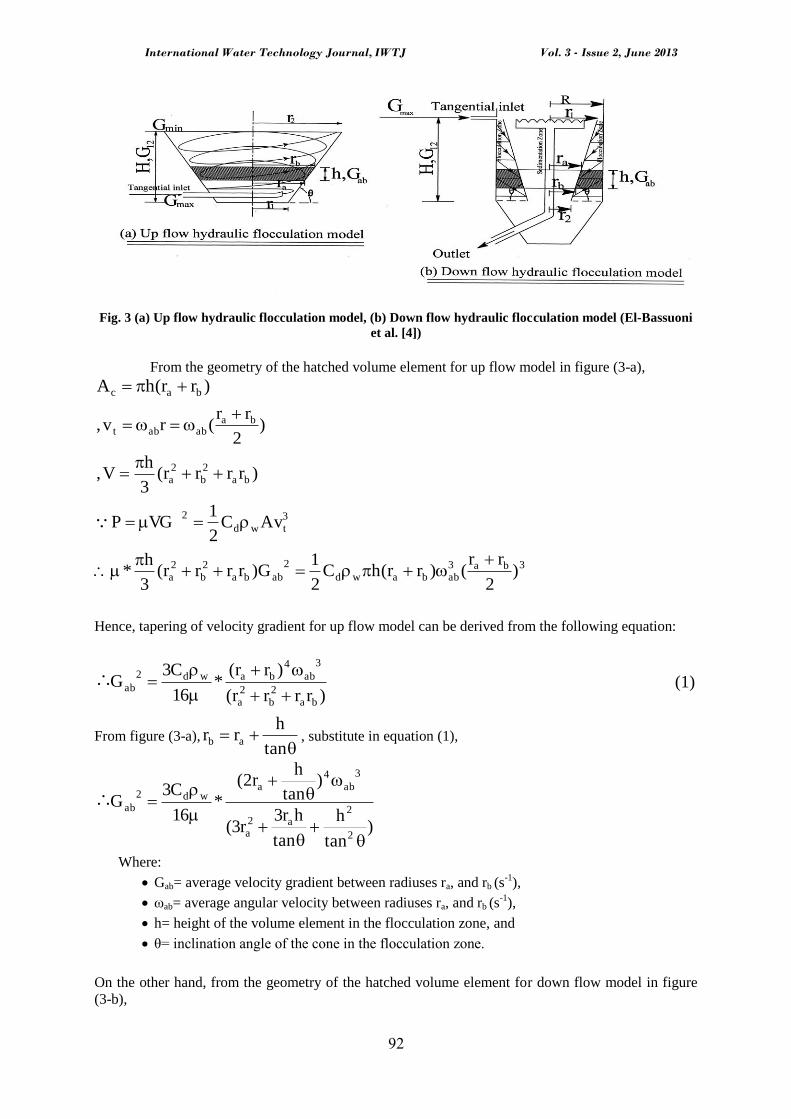
Figures (3-a), and (3-b) represent models of hydraulic flocculators using swirl flow; the design
equation of a swirl flow hydraulic flocculators for each model can be derived as the following:
International Water Technology Journal, IWTJ Vol. 3 - Issue 2, June 2013
89
Fig. 3 (a) Up flow hydraulic flocculation model, (b) Down flow hydraulic flocculation model (El-Bassuoni
et al. [4])
From the geometry of the hatched volume element for up flow model in figure (3-a),
)rr(hA bac
)2
rr(rv, ba
ababt
)rrrr(3
hV, ba
2
b
2
a
3
twd
2AvC
2
1VGP
3ba3
abbawd
2
abba
2
b
2
a )2
rr()rr(hC
2
1G)rrrr(
3
h*
Hence, tapering of velocity gradient for up flow model can be derived from the following equation:
)rrrr(
)rr(*
16
C3G∴
ba2b
2a
3
ab
4
bawd2
ab
(1)
From figure (3-a),
tan
hrr ab , substitute in equation (1),
)tan
h
tan
hr3r3(
)tan
hr2(
*16
C3G∴
2
2a2
a
3
ab4
awd2
ab
Where:
Gab= average velocity gradient between radiuses ra, and rb (s-1
),
ωab= average angular velocity between radiuses ra, and rb (s-1
),
h= height of the volume element in the flocculation zone, and
θ= inclination angle of the cone in the flocculation zone.
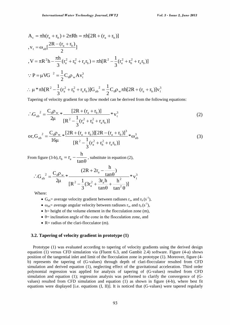
On the other hand, from the geometry of the hatched volume element for down flow model in figure
(3-b),
International Water Technology Journal, IWTJ Vol. 3 - Issue 2, June 2013
89
)]rr(R2[hRh2)rr(hA babac
]2
)rr(R2[v, ba
abt
)]rrrr(3
1R[h)rrrr(
3
hhRV, ba
2
b
2
a
2
ba
2
b
2
a
2
3
twd
2AvC
2
1VGP
3
tbawd
2
abba
2
b
2
a
2 v)]rr(R2[hC2
1G)]rrrr(
3
1R[h*
Tapering of velocity gradient for up flow model can be derived from the following equations:
3
t
ba
2
b
2
a
2
bawd2
ab v*
)]rrrr(3
1R[
)]rr(R2[*
2
CG∴
(2)
3
ab
ba
2
b
2
a
2
3
babawd2
ab *
)]rrrr(3
1R[
)]rr(R2)][rr(R2[*
16
CG,or
(3)
From figure (3-b),
tan
hrr ab , substitute in equation (2),
3
t
2
2a2
a
2
awd2
ab v*
)]tan
h
tan
hr3r3(
3
1R[
)tan
hr2R2(
*2
CG∴
Where:
Gab= average velocity gradient between radiuses ra, and rb (s-1
),
ωab= average angular velocity between radiuses ra, and rb (s-1
),
h= height of the volume element in the flocculation zone (m),
θ= inclination angle of the cone in the flocculation zone, and
R= radius of the clari-flocculator (m).
3.2. Tapering of velocity gradient in prototype (1)
Prototype (1) was evaluated according to tapering of velocity gradients using the derived design
equation (1) versus CFD simulation via (Fluent 6.3, and Gambit 2.4) software. Figure (4-a) shows
position of the tangential inlet and limit of the flocculation zone in prototype (1). Moreover, figure (4-
b) represents the tapering of (G-values) through depth of clari-flocculator resulted from CFD
simulation and derived equation (1), neglecting effect of the gravitational acceleration. Third order
polynomial regression was applied for analysis of tapering of (G-values) resulted from CFD
simulation and equation (1); regression analysis was performed to clarify the convergence of (G-
values) resulted from CFD simulation and equation (1) as shown in figure (4-b), where best fit
equations were displayed [i.e. equations (I, II)]. It is noticed that (G-values) were tapered regularly

International Water Technology Journal, IWTJ Vol. 3 - Issue 2, June 2013
89
through flocculation zone depth with rate of 39.5 s-1
/m depth [using CFD simulation] versus 32.5 s-1
/m
depth [using equation (1)].
On the other hand, CFD simulation was processed considering the gravitational acceleration; (G-
values) were relatively declined in comparison with neglecting effect of the gravitational acceleration.
Hence, gravitational acceleration result noticeable differences in velocity gradient (ΔG) through depth
of the flocculation zone (d); then, correction of velocity gradient (ΔG) can be determined using of
dimensional analysis as follows: ba
g dkg)d,g(fGGG
Where:
ΔG = velocity gradient resulted from effect of the gravitational acceleration (s-1
),
Gg= (G- values) with considering of the gravitational acceleration (s-1
),
G= (G- values) with neglecting of the gravitational acceleration (s-1
),
g= gravitational acceleration =9.81m/s2,
d= flocculation depth, measured from the tangential inlet level (m), and
k= an empirical coefficient deduced in section (3.4).
The previous equation must be dimensionally homogenous; the exponents of each of the quantities
must be the same on each side of the equation; a2baba21 )T()L()L()LT(T
5.0b,5.0a
d
gkG (4)
The corrected velocity gradient (Gg-values) can be determined by modifying equation (1) as follows:
d
gk
)rrrr(
)rr(*
16
C3)G(
ba
2
b
2
a
3
ab
4
bawdgab
(5)
In case of prototype (1), k= -1.9. As shown in figure (4-b), (G-values) were corrected using the
modified design equation (5). Also, regression analysis was applied for the corrected values to clarify
the convergence of (G- values) resulted from CFD simulation (considering gravitational acceleration),
and derived equation (5) as shown in figure (4-b), where best fit equations were displayed [i.e.
equations (III, IV)].
(a)

International Water Technology Journal, IWTJ Vol. 3 - Issue 2, June 2013
89
(b)
Fig. 4 (a) Geometry of prototype (1), (b) (G- values) resulted from CFD simulation and derived design
equations for prototype (1)
3.3. Tapering of velocity gradient in prototype (2)
Prototype (2) was evaluated according to tapering of velocity gradients using the derived design
equations (2, 3) versus CFD simulation via (Fluent 6.3, and Gambit 2.4) software; Figure (5-a) shows
position of the tangential inlet and limit of the flocculation zone in prototype (2). Moreover, figure (5-
b) represents the tapering of (G-values) through depth of clari-flocculator resulted from CFD
simulation and derived equations (2, 3), neglecting effect of the gravitational acceleration. Third order
polynomial regression was applied for analysis of tapering of (G-values) resulted from CFD
simulation and equation (3); regression analysis was performed to clarify the convergence of (G-
values) resulted from CFD simulation and equation (3) as shown in figure (5-b), where best fit
equations were displayed [i.e. equations (I, II)]. It is noticed that (G-values) were tapered through
flocculation zone depth with relatively small rate of 9 s-1
/m depth [using CFD simulation] versus 3.9 s-
1/m depth [using equation (3)].
On the other hand, CFD simulation was processed considering the gravitational acceleration; (G-
values) were relatively increased in comparison with neglecting effect of the gravitational
acceleration. Hence, gravitational acceleration result noticeable differences in velocity gradient (ΔG)
through depth of the flocculation zone (d); then, correction of velocity gradient (ΔG) can be
determined using the previously derived equation (4):
d
gkG
(4)
The corrected velocity gradient (Gg-values) can be determined by modifying equation (3) as follows:
d
gk*
)]rrrr(3
1R[
)]rr(R2)][rr(R2[*
16
C)G( 3
ab
ba2b
2a
2
3babawd
gab
(6)
In case of prototype (2), k= 3.4. As shown in figure (5-b), (G-values) were corrected using the
modified design equation (6). Also, regression analysis was achieved for the corrected values to clarify
the convergence of (G-values) resulted from CFD simulation (considering gravitational acceleration),

International Water Technology Journal, IWTJ Vol. 3 - Issue 2, June 2013
89
and derived equation (6) as shown in figure (5-b), where best fit equations were displayed [i.e.
equations (III, IV)].
(a)
(b)
Fig. 5 (a) Geometry of prototype (2), (b) (G- values) resulted from CFD simulation and derived design
equations for prototype (2)
3.4. Estimation of velocity gradient resulting from the gravitational acceleration
Empirical coefficient (k) resulted from the dimensional analysis as explained in equation (4), can
be deduced by comparing (G-values) resulted from CFD simulation in cases of neglecting and
considering effect of the gravitational acceleration; CFD simulation was processed for different sizes
and configurations of hydraulic clari-flocculators, which ranged between 5m to 40m in diameter.
Consequently, a logarithmic regression was applied for the different results to predict the best fit
equations as shown in figure (6), where the empirical coefficient (k) can be determined for the
different types and dimensions of swirl flow hydraulic clari-flocculators.

International Water Technology Journal, IWTJ Vol. 3 - Issue 2, June 2013
89
From equations (5,6), the corrected velocity gradient (Gg-values) can be determined using the
following equations:
For up flow flocculation,
]043.0)5
ln(39.1[d
g
)rrrr(
)rr(*
16
C3)G(
ba
2
b
2
a
3
ab
4
bawdgab
(7)
For down flow flocculation,
]072.0)5
ln(51.2[d
g*
)]rrrr(3
1
4[
)]rr()][rr([*
16
C)G( 3
ab
ba2b
2a
2
3babawd
gab
(8)
Where:
(Gab)g= average velocity gradient between radiuses ra, and rb ,considering the gravitational
acceleration(s-1
),
Cd= drag coefficient of water,
ρw= water density (Kg/m3),
µ= absolute viscosity of the water (Kg.m/s),
Φ= diameter of clari-flocculator (m),
ωab= average angular velocity between radiuses ra, and rb (s-1
),
g= gravitational acceleration =9.81m/s2, and
d= flocculation depth, measured from the tangential inlet level (m).
Fig. 6 Empirical coefficient (k) for up flow and down flow flocculation

International Water Technology Journal, IWTJ Vol. 3 - Issue 2, June 2013
88
3.5. Evaluation of the different prototypes
From the previous results, it is noticed that (G-values) were tapered through flocculation depth with
rate about 33.6 s-1
/m depth, from the different results of prototype (1); While, rate of tapering of (G-
values) was about 8.7 s-1
/m depth, from the different results of prototype (2). This means that rate of
tapering of (G-values) in upward swirl flow (1) roughly equal to 4 times its value in downward swirl
flow, which indicates that gravitational acceleration relatively improves regularity of tapering of (G-
values) for up flow flocculation, whereas it declines to some extent the tapering of (G-values) for
down flow flocculation, where (G-values) seemed to be almost constant. Therefore, prototype (1) as a
model of up flow hydraulic clari-flocculator is preferable as a modification of the conventional
primary sedimentation tank to accommodate excess flow rate of sewage.
On the other hand, the barrier between the flocculation and clarification zones in the prototype (2)
adds a comparative advantage compared with prototype (1) summarized in retaining of the formed
flocs from cracking. In addition, downward swirl flow [prototype (2)] also features the upward swirl
flow [prototype (1)] in the presence of sludge hopper at the bottom of the tank, which is poised to
receive all sludge in the tank; while, the position of the sludge hopper over the flocculation zone in
prototype (1) enables the small sediments to escape to the bottom of the tank, and it may be mixed
with the raw sewage till increasing the concentration of the pollutants. Consequently, it may reduce
the treatment efficiency. Therefore, prototype (2) is suitable for potable water purification to ensure
the separation between flocculation and sedimentation processes, as well as prototype (2) may be
appropriate for upgrading the sewage treatment plants designed without primary sedimentation (e.g.
oxidation ditches system); while, prototype (1) is suitable for the enhancement of the primary
treatment of sewage, especially, in the already existing plants which contain primary sedimentation
tanks.
4. CONCLUSIONS
The obtained results reveal the following conclusions:
The tapering of velocity gradient is more regular in upward swirl flow rather than downward swirl
flow.
Gravitational acceleration relatively improves regularity of tapering of (G-values) for up flow
flocculation, whereas it declines to some extent the tapering of (G-values) for down flow
flocculation, where (G-values) seemed to be almost constant.
The barrier between the flocculation and clarification zones in the prototype (2) adds a
comparative advantage compared with prototype (1) summarized in retaining of the formed flocs
from cracking.
Downward swirl flow [prototype (2)] also features the upward swirl flow [prototype (1)] in the
presence of sludge hopper at the bottom of the tank, which is poised to receive all sludge in the
tank; while, the position of the sludge hopper over the flocculation zone in prototype (1) enables
the small sediments to escape to the bottom of the tank, and it may be mixed with the raw sewage
till increasing the concentration of the pollutants. Consequently, it may reduce the treatment
efficiency. Therefore, prototype (2) is suitable for potable water purification to ensure the
separation between flocculation and sedimentation processes, as well as prototype (2) may
upgrade the sewage treatment plants designed without primary sedimentation (e.g. oxidation
ditches system); while, prototype (1) is suitable for the enhancement of the primary treatment of
sewage, especially, in the already existing plants which contains primary clarifiers.

International Water Technology Journal, IWTJ Vol. 3 - Issue 2, June 2013
88
REFRENCES
[1] Younis, S.S; Al Mansi, N.M; and Fouad, S.H. (1998). “Chemically assisted primary treatment of
municipal wastewater”. Journal of Environmental Management and Health p.p:209-214.
[2] Rashed, I.G; El-Komy, M. A; Al-Sarawy, A. A; and Al-Gamal, H. F, (1997). “Chemical Treatment
of Sewage"; the First Scientific Conference of the Egyptian Society for the Development of Fisheries
Resources and Human Health, El Arish, Egypt.
[3] Engelhardt, T.L. (2010). “Coagulation, Flocculation and Clarification of Drinking Water”.
Drinking water sector, Hach Company.
[4] El-Bassuoni, A.A; Rashed, I.G.; Al-Sarawy, A.A; and El-Halwany, M.M.(2005). “A Novel
Compact Coagulation-Flocculation-Sedimentation System”. 9th International Water Technology
Conference, Sharm El-Sheikh, Egypt.
[5] Richardson, J.F; Harker, J.H; and Backhurst, J.R. (2002). “Chemical Engineering Series: Particle
Technology and Separation Processes”. Volume (2). Butterworth- Heinemann, Oxford.
[6] Crittenden, J.C; Trussel,R.R; Hand, D.W. ; Howe, K.J; and Tchobanoglous, G.(2005) “ Water
Treatment Principles and Design” second edition , Jhon Wiley and Sons Inc.
[7] McCable, W.L; Smith, J.C; and Harriott, P. (1993). “Unit Operation of Chemical Engineering”. 5th
edition. McGraw Hill.
[8] Chiang, S.H. (2005). “Solid- Liquid Separation”. CRC Press LLC.
[9] Davailles, A; Climent, E; and Bourgeois, F.(2012). “Fundamental understanding of swirling flow
pattern in hydrocyclones”. Separation and Purification Technology, Vol.92. pp. 152-160. ISSN 1383-
5866.
[10] Xu, Peng; Wu, Zhonghua; and Mujumdar, Aruns. (2009). “Mathematical Modelling of Industrial
Transport Processes”. National University of Singapore.
[11] Brennan, M; Holtham, P; and Narasimha, M. (2009) “CFD Modelling of Cyclone Separator:
Validation against plant hydrodynamics performance”. 7th International Conference on CFD in the
Minerals and Process Industries, CSIRO, Melbourne, Australia.
[12] Yuan Hsu, Chih; Jhih Wu, Syuan; and Ming Wu, Rome. (2011). “Particles Separation and Tracks
in Hydrocyclone”. Tamkang Journal of Science and Engineering, Vol.14, No.1, pp. 65-70.
[13] Anderson, J.D. (1995). “Computational Fluid Dynamics: The Basics with Applications”.
Mechanical Engineering Series. Mc Graw- Hill International Editions. ISBN 0-07-113210-4.
[14] Bridgeman, J; Jefferson, B; and Parson, S.A. (2009). “Computational Fluid Dynamics Modelling
of Flocculation in Water Treatment: A Review”. Engineering Applications of Computational Fluid
Mechanics. Vol. 3, No.2, pp.220-241.
[15] Metcalf & Eddy, Inc., George Tchobanoglous; Franklin L. Burton; and H. David Stensel. (2003).
“Wastewater Engineering Treatment and Reuse” 4th ed., Mc Graw-Hill.
[16] Rashed, I.G; Afify, H. A; Ahmed, A.E; and Ayoub, M. A. (2013). “Optimization of chemical
precipitation to improve the primary treatment of wastewater”. Journal of Desalination and Water
Treatment, USA. (In press).