hydraulic modelling of unsteady open channel flow ...263564/s42385743_mphil... · hydraulic...

Hydraulic Modelling of Unsteady Open Channel Flow: Physical and

Analytical Validation of Numerical Models of Positive and Negative

Surges

Martina Reichstetter

A thesis submitted for the degree of Master of Philosophy at

The University of Queensland in August 2011

School of Civil Engineering

ii

Declaration by author

This thesis is composed of my original work, and contains no material previously published

or written by another person except where due reference has been made in the text. I

have clearly stated the contribution by others to jointly-authored works that I have included

in my thesis.

I have clearly stated the contribution of others to my thesis as a whole, including statistical

assistance, survey design, data analysis, significant technical procedures, professional

editorial advice, and any other original research work used or reported in my thesis. The

content of my thesis is the result of work I have carried out since the commencement of

my research higher degree candidature and does not include a substantial part of work

that has been submitted to qualify for the award of any other degree or diploma in any

university or other tertiary institution. I have clearly stated which parts of my thesis, if any,

have been submitted to qualify for another award.

I acknowledge that an electronic copy of my thesis must be lodged with the University

Library and, subject to the General Award Rules of The University of Queensland,

immediately made available for research and study in accordance with the Copyright Act

1968.

I acknowledge that copyright of all material contained in my thesis resides with the

copyright holder(s) of that material.

iii

Statement of Contributions to Jointly Authored Works Contained in the Thesis

“No jointly-authored works.”

Statement of Contributions by Others to the Thesis as a Whole

“No contributions by others.”

Statement of Parts of the Thesis Submitted to Qualify for the Award of Another

Degree

“None.”

Published Works by the Author Incorporated into the Thesis

“None.”

Additional Published Works by the Author Relevant to the Thesis but not Forming

Part of it

REICHSTETTER, M., and CHANSON, H. (2011). "Negative Surge in Open Channel:

Physical, Numerical and Analytical Modelling." Proc. 34th IAHR World Congress,

Brisbane, Australia, 26 June-1 July, Engineers Australia Publication, Eric VALENTINE,

Colin APELT, James BALL, Hubert CHANSON, Ron COX, Rob ETTEMA, George

KUCZERA, Martin LAMBERT, Bruce MELVILLE and Jane SARGISON Editors, pp.2306-

2313.

iv

Acknowledgements

This research project would not have been possible without the support of many people.

The author wishes to express her gratitude to her supervisor, Prof. Hubert Chanson who

was abundantly helpful and offered invaluable assistance, support and guidance.

Besides my advisor, the author would like to thank my assistant advisor Dr. Luke Toombes

for his encouragement and technical support.

Sincere thanks also go to Professor Peter Rutschmann and his team for offering me the

exchange opportunity at the Technical University of Munich sharing his resources and

expertise. The author would like to express her thanks to Michael Seitz and Shokry

Abdelaziz for their support during my stay at the Technical University of Munich.

The author likes to express her gratitude to Dr. Pierre Lubin of the University of Bordeaux

for his help and sharing his vast expertise in CFD modeling and formatting of a successful

conference presentation.

The author thanks her fellow researchers in the School of Civil Engineering at UQ for the

stimulating discussions, especially my office mate Stefan Felder.

Last but not the least; the author would like to thank her family, her parents Hermann

Reichstetter and Elisabeth, for supporting her throughout life.

v

Abstract

Positive and negative surges are generally observed in open channels. Positive surges

that occur due to tidal origins are referred to as tidal bores. A positive surge occurs when a

sudden change in flow leads to an increase of the water depth, while a negative surge

occurs due to a sudden decrease in water depth. Positive and negative surges are

commonly induced by control structures, such as the opening and closing of a gate. In this

study, the free-surface properties and velocity characteristics of negative and positive

surges were investigated physically under controlled conditions, as well as analytically and

numerically. Unsteady open channel flow data were collected during the upstream

propagation of negative and positive surges. Both, physical and numerical modelling, were

performed. Some detailed measurements of free-surface fluctuations were recorded using

non-intrusive techniques, including acoustic displacement meters and video recordings.

Velocity measurements were sampled with high temporal and spatial resolution using an

ADV (200 Hz) at four vertical elevations and two longitudinal locations. The velocity and

water depth results were ensemble-averaged for both negative and positive surges. The

results showed that the water curvature of the negative surge was steeper near the gate at

x=10.5 m compared to further upstream at x=6 m. Both the instantaneous and ensemble-

average data showed that in the negative surge the inflection point of the water surface

and the longitudinal velocity Vx occurred simultaneously. Also, an increase in Vx was

observed at all elevations during the surge passage. For the positive surge the

propagation of the bore and the velocity characteristics supported earlier findings by Koch

and Chanson (2009) and Docherty and Chanson (2010). The surge was a major

discontinuity in terms of the free-surface elevations, and a deceleration of the longitudinal

velocities Vx was observed during the surge passage. A number of analytical and

numerical models were tested, including the analytical and numerical solutions of the

Saint-Venant equations and a computational fluid dynamics (CFD) package. Overall, all

models provided reasonable results for the negative surge. None of the models were able

to provide a good agreement with the measured data for the positive surge. The study

showed that theoretical models may be applied successfully to unsteady flow situations

with simple channel geometry. Also, it was found that the selection of the appropriate

mesh size for CFD simulations is essential in highly unsteady turbulent flows, such as a

positive surge, where the surge front is a sharp discontinuity in terms of water elevation,

velocity and pressure. It was concluded that the highly unsteady open channel flows

remain a challenge for professional engineers and researchers.

vi

Keywords

modelling, unsteady open channel flows, positive surges, negative surges, physical

modelling, numerical modelling, theoretical modelling, Saint-Venant equations, laboratory

experiments, computational fluid dynamics (CFD)

Australian and New Zealand Standard Research Classifications (ANZSRC)

090509 Water Resources Engineering

vii

Table of Contents

ABSTRACT ....................................................................................................................................................... V

NOTATION ...................................................................................................................................................... XII

1 INTRODUCTION ....................................................................................................................................... 1

1.1 DESCRIPTION ..................................................................................................................................... 1

1.2 OBJECTIVES AND OUTLINE ................................................................................................................... 2

2 POSITIVE AND NEGATIVE SURGES: A BIBLIOGRAPHIC REVIEW .................................................... 3

2.1 PRESENTATION ................................................................................................................................... 3

2.2 BASIC EQUATIONS ............................................................................................................................... 4

2.3 ANALYTICAL SOLUTION OF THE SAINT-VENANT EQUATIONS ................................................................... 4

2.4 PREVIOUS EXPERIMENTAL RESEARCH .................................................................................................. 5

2.5 PREVIOUS NUMERICAL RESEARCH ....................................................................................................... 9

3 EXPERIMENTAL SETUP ........................................................................................................................12

3.1 EXPERIMENTAL FACILITY ................................................................................................................... 13

3.2 INSTRUMENTATION ............................................................................................................................ 13

3.2.1 Free surface measurements using acoustic displacement meters ............................................ 14

3.2.2 Free surface profile using video imagery ................................................................................... 14

3.2.3 Velocity fluctuations measurements using acoustic Doppler velocimeter (ADV) ...................... 15

3.2.4 Experimental procedure and flow conditions ............................................................................. 17

4 EXPERIMENTAL RESULTS ...................................................................................................................20

4.1 ACOUSTIC DOPPLER VELOCIMETER AND ACOUSTIC DISPLACEMENT METER RESULTS ............................ 20

4.1.1 Negative surge ........................................................................................................................... 20

4.1.2 Positive surge............................................................................................................................. 24

4.2 VIDEO ANALYSIS RESULTS ................................................................................................................. 25

4.2.1 Negative surge ........................................................................................................................... 26

4.2.2 Positive surge............................................................................................................................. 29

4.3 ENSEMBLE-AVERAGE RESULTS .......................................................................................................... 33

4.3.1 Negative surge ........................................................................................................................... 33

4.3.2 Positive surge............................................................................................................................. 38

4.4 DISCUSSION ..................................................................................................................................... 44

5 NUMERICAL MODELLING .....................................................................................................................46

5.1 ONE DIMENSIONAL MODELLING: NUMERICAL SOLUTION OF THE SAINT-VENANT EQUATIONS ................... 46

5.1.1 Negative surge ........................................................................................................................... 46

5.1.2 Positive surge............................................................................................................................. 48

5.2 TWO DIMENSIONAL MODELLING WITH FLOW-3D .................................................................................. 49

5.2.1 Negative surge ........................................................................................................................... 50

5.2.2 Positive surge............................................................................................................................. 52

viii

6 COMPARISON BETWEEN NUMERICAL AND PHYSICAL DATA .......................................................55

6.1 NEGATIVE SURGE ............................................................................................................................. 55

6.1.1 Surface profile ............................................................................................................................ 55

6.1.2 Turbulent velocities .................................................................................................................... 56

6.2 POSITIVE SURGE ............................................................................................................................... 59

6.2.1 Surface profile ............................................................................................................................ 59

6.2.2 Turbulent velocities .................................................................................................................... 60

7 CONCLUSION .........................................................................................................................................62

REFERENCES .................................................................................................................................................65

APPENDIX A – PHOTOGRAPHS OF THE EXPERIMENTS ............................................................................ 1

APPENDIX B - ENSEMBLE-AVERAGE RESULTS - NEGATIVE SURGE ...................................................... 6

APPENDIX C - ENSEMBLE-AVERAGE RESULTS – POSITIVE SURGE .....................................................15

APPENDIX D – FLOW-3D SETUP AND RESULTS .......................................................................................18

APPENDIX E - CELERITY ...............................................................................................................................23

APPENDIX F – STEADY STATE FLOW PROFILES ......................................................................................26

ix

List of Figures

FIGURE 1-1: PHOTOGRAPHS OF A NEGATIVE AND POSITIVE SURGE ..................................................................................................... 1

FIGURE 2-1: DEFINITION SKETCH OF (A) POSITIVE SURGE AND (B) NEGATIVE SURGE .............................................................................. 3

FIGURE 3-1: PHOTOGRAPHS OF EXPERIMENTAL SETUP (A) X=6 M, (B) X=10.5 M AND (C) X=0-12 M (COURTESY OF PROF. HUBERT CHANSON)

................................................................................................................................................................................. 13

FIGURE 3-2: CALIBRATION RESULTS FOR THE DISPLACEMENT METER MEASUREMENTS ......................................................................... 14

FIGURE 3-3: SKETCH OF THE VIDEO SETUP .................................................................................................................................. 15

FIGURE 3-4: ACOUSTIC DOPPLER VELOCIMETER (ADV) ................................................................................................................ 16

FIGURE 3-5: SKETCH OF EXPERIMENTAL SET-UP WITH ADV ........................................................................................................... 18

FIGURE 4-1: DIMENSIONLESS INSTANTANEOUS VELOCITY AND DEPTH MEASUREMENTS OF A NEGATIVE SURGE AT X=10.5 M ...................... 21

FIGURE 4-2: DIMENSIONLESS INSTANTANEOUS VELOCITY AND DEPTH MEASUREMENTS OF A NEGATIVE SURGE AT X=6 M............................ 23

FIGURE 4-3: DIMENSIONLESS INSTANTANEOUS VELOCITY AND DEPTH MEASUREMENTS OF A POSITIVE SURGE AT X=6 M ............................. 24

FIGURE 4-4: DIMENSIONLESS INSTANTANEOUS VELOCITY AND DEPTH MEASUREMENTS OF A POSITIVE SURGE AT X=10.5 M ........................ 25

FIGURE 4-5: PHOTOS OF (A) POSITIVE AND (B) NEGATIVE SURGE NEAR THE GATE AT (11.2 M< X <10.48 M) .......................................... 26

FIGURE 4-6: DIMENSIONLESS VIDEO DATA FOR THE NEGATIVE SURGE IMMEDIATELY U/S OF THE GATE 10.5 M, WITH X’=0 CORRESPONDING TO

X=11.2 M .................................................................................................................................................................. 27

FIGURE 4-7: DIMENSIONLESS VIDEO DATA FOR THE NEGATIVE SURGE AT 6 M, WITH X’=0 CORRESPONDING TO X=6.3 M ........................... 28

FIGURE 4-8: DIMENSIONLESS VIDEO DATA FOR THE POSITIVE SURGE AT 10.5 M, WITH X’=0 CORRESPONDING TO X=11.2 M ..................... 30

FIGURE 4-9: DIMENSIONLESS VIDEO DATA FOR THE POSITIVE SURGE AT 6 M, WITH X’=0 CORRESPONDING TO X=6.9 M ............................ 31

FIGURE 4-10: INSTANTANEOUS AND MEDIAN DATA FOR ALL 25 RUNS FOR THE NEGATIVE SURGE AT Z=6.69 MM .................................... 34

FIGURE 4-11: DIMENSIONLESS ENSEMBLE-AVERAGE MEDIAN WATER DEPTH DMEDIAN, DIFFERENCE BETWEEN 3RD AND 4TH QUARTILES (D75-

D25) AND 90% AND 10% PERCENTILES (D90-D10), AND RANGE OF MAXIMUM TO MINIMUM WATER DEPTH (DMAX-DMIN) ........... 35

FIGURE 4-12: DIMENSIONLESS ENSEMBLE-AVERAGE MEDIAN VELOCITY VMEDIAN, DIFFERENCE BETWEEN 3RD AND 4TH QUARTILES (V75-

V25) AND 90% AND 10% PERCENTILES (V90- V10), AND RANGE OF MAXIMUM TO MINIMUM WATER DEPTH (VMAX- VMIN) AT X=6 M

AND Z=6.69 MM ......................................................................................................................................................... 36


V25) AND 90% AND 10% PERCENTILES (VZ90- VZ10), AND RANGE OF MAXIMUM TO MINIMUM WATER DEPTH (VMAX- VMIN) AT

X=10.5 M AND Z=6.69 MM........................................................................................................................................... 37

FIGURE 4-14: INSTANTANEOUS AND MEDIAN DATA FOR THE POSITIVE SURGE AT X=6M AND Z=6.69 MM .............................................. 39

FIGURE 4-15: DIMENSIONLESS ENSEMBLE-AVERAGE MEDIAN WATER DEPTH DMEDIAN, DIFFERENCE BETWEEN 3RD AND 4TH QUARTILES (D75-

D25) AND 90% AND 10% PERCENTILES (D90-D10), AND RANGE OF MAXIMUM TO MINIMUM WATER DEPTH (DMAX-DMIN) ............ 41


V25) AND 90% AND 10% PERCENTILES (V90- V10), AND RANGE OF MAXIMUM TO MINIMUM WATER DEPTH (VMAX- VMIN) AT X=6 M

AND Z=6.69 MM. ........................................................................................................................................................ 42


V25) AND 90% AND 10% PERCENTILES (VZ90- VZ10), AND RANGE OF MAXIMUM TO MINIMUM WATER DEPTH (VMAX- VMIN) AT

X=10.5 M AND Z=6.69 MM........................................................................................................................................... 43

FIGURE 4-18: CELERITY OF NEGATIVE SURGES ............................................................................................................................. 45

FIGURE 5-1: NUMERICAL INTEGRATION OF THE METHODS OF CHARACTERISTICS BY THE HARTREE METHODS ........................................... 47

x

FIGURE 5-2: DIMENSIONLESS UNSTEADY FREE-SURFACE PROFILE DURING THE NEGATIVE SURGE WITH 20 L/S DISCHARGE AND A 30 MM GATE

OPENING .................................................................................................................................................................... 48

FIGURE 5-3: DIMENSIONLESS UNSTEADY FREE-SURFACE PROFILE DURING THE POSITIVE SURGE WITH 20 L/S DISCHARGE AND A 30 MM GATE

OPENING .................................................................................................................................................................... 48

FIGURE 5-4: DIMENSIONLESS UNSTEADY FREE-SURFACE PROFILE DURING THE NEGATIVE SURGE RECORDED AND SIMULATED DATA ............... 51

FIGURE 5-5: DIMENSIONLESS VELOCITY AND DEPTH MEASUREMENTS OF A NEGATIVE SURGE SIMULATED USING FLOW-3D ......................... 52

FIGURE 5-6: DIMENSIONLESS UNSTEADY FREE-SURFACE PROFILE DURING THE POSITIVE SURGE RECORDED AND SIMULATED DATA ................ 53

FIGURE 5-7: DIMENSIONLESS VELOCITY AND DEPTH MEASUREMENTS OF A POSITIVE SURGE SIMULATED USING FLOW-3D AT X=6 M, Z=7.5 MM,

Q=20 L/S, D0=0.064 M, INITIAL GATE OPENING 30 MM AND 5 MM MESH SIZE ....................................................................... 54

FIGURE 6-1: DIMENSIONLESS UNSTEADY FREE-SURFACE PROFILE DURING THE NEGATIVE SURGE WITH Q=20 L/S AND A 30 MM GATE OPENING

................................................................................................................................................................................. 56

FIGURE 6-2: COMPARISON OF THE DIMENSIONLESS LONGITUDINAL VELOCITY COMPONENTS VX DERIVED FROM ANALYTICAL AND NUMERICAL

METHODS WITH MEASURED DATA AT X=6 M - FLOW-3D CALCULATIONS PERFORMED WITH 5 MM MESH SIZE . ............................... 58

FIGURE 6-3: UNSTEADY FREE-SURFACE PROFILE DURING THE POSITIVE SURGE .................................................................................... 60

FIGURE 6-4: COMPARISON OF THE DIMENSIONLESS LONGITUDINAL VELOCITY COMPONENTS VX DERIVED FROM ANALYTICAL AND NUMERICAL

METHODS WITH MEASURED DATA AT X=6 M - FLOW-3D CALCULATIONS PERFORMED WITH 5 MM MESH SIZE. ................................ 61

xi

List of Tables

TABLE 2-1: PREVIOUS EXPERIMENTAL RESEARCH INTO POSITIVE SURGES AND TIDAL BORES ..................................................................... 7

TABLE 2-2: PREVIOUS EXPERIMENTAL INVESTIGATION INTO DAM BREAK WAVES ................................................................................... 8

TABLE 3-1: EXPERIMENTAL FLOW CONDITIONS FOR TURBULENT VELOCITY MEASUREMENTS .................................................................. 19

TABLE 4-1: STEADY STATE EXPERIMENTAL FLOW CONDITIONS FOR ADV AND ADM MEASUREMENTS ..................................................... 20

TABLE 4-2: EXPERIMENTAL FLOW CONDITIONS FOR WATER SURFACE MEASUREMENTS USING VIDEO ANALYSIS ......................................... 26

TABLE 4-3: FLOW CONDITIONS AND CELERITY MEASUREMENT ........................................................................................................ 45

TABLE 5-1: BOUNDARY CONDITIONS FOR FLOW-3D MODELS ......................................................................................................... 50

xii

Notation

The following symbols are used in this report:

A flow cross-section area (m2);

B free-surface width (m);

C wave celerity (m/s);

Co initial celerity (m/s) of a small disturbance in the reservoir with initial

reservoir depth do;

d flow depth (m) measured normal to the invert;

do initial reservoir height (m) measured normal to the chute invert;

DH hydraulic diameter (m);

Fr 1- flow Froude number: Fr=V/ ;

2- surge Froude number: Fr=(V+U)/ ;

f Darcy-Weisbach friction factor;

g gravity constant: g=9.8 m/s2;

L channel length (m);

Pw wetted perimeter (m);

Q volume flow rate (m3/s);

Sf friction slope;

So bed slope: So=sinθ;

t time (s);

U surge celerity (m/s) positive u/s;

V flow velocity (m/s);

Vo initial flow velocity (m/s);

Vx flow velocity component (m/s) in x-direction;

xiii

Vy flow velocity component (m/s) in y-direction;

Vz flow velocity component (m/s) in z-direction;

W channel width (m);

x longitudinal distance (m) measured from the upstream end;

x' dimensionless variable;

z vertical elevation (m);

Greek symbols

θ bed slope angle;

o initially steady flow conditions in the channel;

Notation

D/Dt absolute differential;

∂/∂y partial differentiation with respect to y;

Abbreviations

U/S upstream;

D/S downstream;

ADV acoustic Doppler velocimeter;

ADM acoustic displacement meter;

CFD computational fluid dynamics.

1

1 Introduction

1.1 Description

A positive surge occurs when a sudden change in flow leads to an increase of the water

depth. On the other hand, a negative surge occurs due to a sudden decrease in water

depth (Figure 1- 1). Positive and negative surges are commonly induced by control

structures, such as the opening and closing of a gate respectively (e.g. Henderson 1966,

Chanson 2004). Positive and negative surges are generally observed in man-made

channels. Positive surges that occur due to tidal origins are referred to as tidal bores

(Chanson 2010). Surge waves resulting from dam breaks have been responsible for great

destruction. The surge front as a result of a shock, like the complete closing or opening of

a gate, is characterised by a sudden discontinuity and extremely rapid variations of flow

depth and velocity. Many studies have been conducted looking at surges under controlled

laboratory conditions.

Figure 1-1: Photographs of a negative and positive surge

2

Many predictions of surge waves rely on numerical analysis, which are often validated

against limited data sets. The complex flow situations are solved using empirical

approximation and numerical models, which are based on derivates of basic principles,

such as the backwater equation, Saint-Venant and Navier-Stokes equations. Numerical

models are required to make some form of approximation to solve these principles.

Consequently, all models have their limitations. To date most limitations are neither well

understood nor documented.

1.2 Objectives and outline

In this study, the free-surface properties and the velocity characteristics of negative and

positive surges are investigated physically under controlled conditions, as well as

analytically and numerically. New physical modelling is carried out for the specific purpose

to provide benchmark data for numerical model validation. A number of numerical models

are tested, including the integration of the Saint-Venant equations and a more advanced

CFD package. The validation of the numerical models is examined in the cases of positive

and negative surges, including the verification of the model predictions against physical

model data.

The aim of this work is to present the background and theory, as well as the results of the

experimental and numerical investigation undertaken on positive and negative surges.

This report describes a series of experimental and numerical analyses of positive and

negative surges. In the next section, a short overview of previous research for negative

and positive surges is presented. In section 3, the experimental setup is presented.

Section 4 lists and discusses the experimental results. In section 5 the numerical model

setup and results are presented. Comparisons of numerical and physical results are

presented and discussed in section 6. Conclusions are presented in section 7.

3

2 Positive and negative surges: a bibliographic review

2.1 Presentation

Water flows can be divided into two flow regimes, steady flows and unsteady flows. In

steady flows the velocity and depth do not change with time at a given location in a

channel. In unsteady flows the flow parameters change with time and location. Unsteady

flows are frequently observed in water supply systems, hydropower canals, and channels

with junctions, as well as dam-breaks. In a channel filled with water, the sudden increase

in water depth is referred to as a positive surge, while the negative surge is characterised

by a reduction in water depth. Historically, some major contributions on surges were

published by Bazin (1865), Barré de Saint Venant (1871) and Boussinesq (1877). More

recently, some unsteady velocity measurements were conducted using acoustic Doppler

velocimeters (ADV) (Koch and Chanson 2009, Chanson 2010, 2011). Figure 2-1(a) shows

the definition sketch of a positive surge for an observer standing on the bank. Figure 2-1

(b) shows the definition sketch of a negative surge.

(a) Definition sketch of a positive surge (Chanson 2004)

(b) Definition sketch of a negative surge (Chanson 2004)

Figure 2-1: Definition sketch of (a) positive surge and (b) negative surge

4

2.2 Basic equations

In unsteady open channel flows, water depth and velocities change with time and

longitudinal position. The Saint-Venant equations consist of the momentum and continuity

equations and are used in the calculation of one-dimensional free-surface flows. The basic

assumptions of the Saint-Venant equation are: (1) the flow is one dimensional; (2) the

streamline curvature is small and the pressure distribution is hydrostatic; (3) the flow

resistance is the same as for a steady uniform flow with the identical depth and velocity;

(4) the bed slope is small enough so that cosθ ≈ 1 and sinθ ≈ tanθ ≈ 0; (5) constant water

density; the channel has fixed boundaries and air entrainment and sediment motion are

neglected (Chanson 2004). Considering these assumptions, every point at all time during

the progression of the surge can be characterised by two variables, such as V and d:

where V is the velocity and d is the water depth. The following system of two partial

differential equations can be used to describe the unsteady flow properties:

0tan

tconsdx

A

B

V

x

dV

x

V

B

A

t

d (2-1)

0)(

of SSg

x

dg

x

VV

t

V (2-2)

where t is the time, A is the cross-section area, B is the free-surface width, x is the

streamwise coordinate, So is the bed slope, θ is the angle between the bed and the

horizontal, with θ > 0 for a downward slope and Sf is the friction slope (Chanson 2004).

The friction slope can be defined as Sf= fv2/(2gDH) where DH is the hydraulic diameter and

the Darcy friction factor f is a non-linear function of both the Reynolds number and the

relative roughness (Chanson 2004). Equation (2-1) is the continuity equation and (2-2) is

the momentum equation (Liggett 1994, Montes 1998, Chanson 2004).

2.3 Analytical solution of the Saint-Venant equations

Simple solutions of the Saint-Venant equations may be obtained using the "simple wave"

approximation. In this study the simple wave method is used to calculate the water surface

profile of the negative wave. A simple wave is defined as a wave for which (So = Sf = 0)

with constant initial water depth and flow velocity (Chanson 2004). To solve the simple

wave, the Saint-Venant equations become a characteristic system of equations:

0)2( CVDt

D forward characteristic (2-3)

5

0)2( CVDt

D backward characteristic (2-4)

along:

CVdt

dx

forward characteristic (2-5)

CVdt

dx

backward characteristic (2-6)

where (V + 2C) is a constant along the forward characteristic (Equation 2-5) (Chanson

2004). For an observer moving at the absolute velocity (V + C), the term (V + 2C) appears

constant. Similarly (V - 2C) appears constant along the backward characteristic (Equation

2-6). The characteristic trajectories are plotted in the (x, t) plane and represent the path of

the observers travelling on the forward and backward characteristics. For each forward

characteristic, the slope of the trajectory is defined as 1/(V + C) and (V + 2C) and is

considered constant along the characteristic trajectory. The characteristic trajectories form

contour lines of (V + 2C) and (V - 2C) (Chanson 2004, Montes 1998). The simple wave

equations were applied to the negative and positive surge experiments and the results are

discussed in section 5.1 and 6. Rapidly varied unsteady flows in open channels, which are

frequently the focus of research studies, include surge waves, stationary or movable

hydraulic jumps and dam-break waves.

2.4 Previous experimental research

Positive surges were studied by a number of researchers for over a century. Relevant

reviews include, but are not limited to Benjamin and Lighthill (1954), Sander and Hutter

(1991), and Cunge (2003). Major contributions were already made early on and included,

but are not limited to the following researchers: Barré de Saint Venant (1871), Boussinesq

(1877), Lemoine (1948) and Serre (1953). The development of the positive surge front was

studied by numerous researchers, such as Tricker (1965), Peregrine (1966), Wilkinson

and Banner (1977), Teles Da Silva and Peregrine (1990), Sobey and Dinemans (1992)

and Koch and Chanson (2009).

6

Most experimental studies were limited to visual observations and occasionally free-

surface measurements, but rarely encompassed velocity fluctuation measurements.

However, there were a few limited studies assessing velocity fluctuation data of positive

surges, such as Yeh and Mok (1990), Hornung et al. (1995), Koch and Chanson (2009)

and Docherty and Chanson (2010). There are too many experimental research projects

focusing on unsteady flows in open channels, to mention, but a selection of the major

studies are summarised in Table 2-1.

While there are numerous experimental studies assessing the positive surge propagation,

there are only few focused on the negative surge propagation and characteristics (Lauber

and Hager 1998, Bazin 1865, Estrade et al.1964, Cavaillé 1965, Dressler 1952).

Dam-break waves are rapidly time variant unsteady flow situations, and research in dam-

break waves may be applicable to positive and negative surge research. While this report

focuses on the positive and negative surges, the author will also discuss previous research

undertaken, on the dam-break wave problem. Most dam- break research was

experimental, much like the research on the positive surge. However, theoretical concepts

and numerical methods are gaining on importance. Relevant studies include, but are not

limited to Schoklitch (1917), Triffonov (1935), De Marchi (1945), Levin (1952), Dressler

(1952, 1954) the US Corps of Engineers (1960), Faure and Nahas (1961), Estrande

(1967), Rajar (1973), Martin (1983), Menendez and Navarro (1990), Lauber (1997) and

Chanson et al. (2000). Table 2-2 lists the main research undertaken in the field of

experimental dam-break research.

7

Notes; do is the initial water depth; Vo is the initial flow velocity; (1) see also Benet and Cunge (1971). Surge type : +

stands for positive surge; - stands for negative surge; U/S stands for moving upstream; D/S stands for moving

downstream (adapted from Koch and Chanson 2005).

Table 2-1: Previous experimental research into positive surges and tidal bores

Reference Vo (m/s) do (m) Surge type

Channel geometry Remarks

Positive Surges

FAVRE (1935) (1) 0 0.106 to 0.206

+ U/S Rectangular (W = 0.42 m) θ = 0º

Laboratory experiments. Flume length : 73.8 m.

≠ 0 0.109 to 0.265

+ U/S Rectangular (W = 0.42 m) θ = 0.017º

ZIENKIEWICZ and SANDOVER (1957)

0.05 to 0.11

+ Rectangular (W = 0.127 m) θ = 0º Smooth flume : glass Rough flume : wire mesh


BENET and CUNGE (1971)

0 to 0.198

0.057 to 0.138

+ D/S Trapezoidal (base width : 0.172 m, sideslope : 2H:1V) θ = 0.021º


0.59 to 1.08

6.61 to 9.16

+ U/S Trapezoidal (base width : 9 m, sideslope : 2H:1V) θ = 0.006 to 0.0086º

Oraison power plant intake channel.

1.51 to 2.31

5.62 to 7.53

+ U/S Trapezoidal (base width : 8.6 m, sideslope : 2H:1V)

Jouques-Saint Estève intake channel.

TRESKE (1994) 0.08 to 0.16

+ U/S Rectangular (W = 1 m) θ = 0.001º

Laboratory experiments. Flume length : 100 m. Concrete channel.

0.04 to 0.16

+ U/S, + D/S

Trapezoidal (base width : 1.24 m, sideslope : 3H:1V) θ = 0º

Laboratory experiments. Flume length: 124 m. Concrete channel.

CHANSON (1995) 0.4 to 1.2

0.02 to 0.15

+ U/S Rectangular (W = 0.25 m) θ = 0.19 to 0.54º Glass walls and bed

Laboratory experiments. Flume length : 20 m.

KOCH and CHANSON (2005)

1.0 0.079 + U/S Rectangular (W = 0.50 m) θ = 0º PVC invert, glass walls

Laboratory experiments. Flume length : 12 m.

Tidal Bores

Dee river, LEWIS (1972)

0 to +0.2 m/s

~ 1.4 m + U/S Dee river near Saltney Ferry footbridge. Trapezoidal channel

Field experiments between March and September 1972.

8

Table 2-2: Previous experimental investigation into dam break waves

Reference Slope deg. Experimental configuration

Schoklitsch (1917)

0

D ≤ 0.25 m, W = 0.6 m

D ≤ 1 m, W = 1.3 m

Triffonov (1935) 0.4 L=30m, W=0.4m

Initial water depth 300 and 400 mm

Dressler (1954) 0 D = 0.055 to 0.22 m, W = 0.225 m

Smooth invert, Sand paper, Slats

Cavaillé (1965) 0 L = 18 m, W = 0.25 m

D = 0.115 to 0.23 m, Smooth invert

D = 0.23 m, Rough invert

Estrade(1967)

0

L = 13.65 m, W =0.50 m

D = 0.2 & 0.4 m, Smooth & Mortar

L = 0.70 m, W = 0.25 m

D = 0.3 m, Smooth & Rough invert

Faure and Nahas (1961) 1.2x10-4

L=40.6 m, W=0.25 m

US Corps of Engineers (1960) 0.5 L=122 m, W=1.22 m

Smooth & Rough

Lauber (1997)

0

L < 3.6 m, W = 0.5 m, D < 0.6 m

Smooth PVC invert

Chanson et al (2000) 0 L=15 m, W=0.8 m

9

2.5 Previous numerical research

Fluid motion is controlled by the principles of conservation of mass, energy and

momentum. Complex flow situations are solved using empirical approximations, as well as

numerical models, which are based on the basic principles, like the Saint-Venant and the

Navier-Stokes equations. All models are required to make an approximation to solve the

basic principles. Therefore, all models have their limitations. Mathematical models

simulating unsteady flows in open channels have been widely used by civil engineers and

other professionals. Computer programs are becoming increasingly available to solve

unsteady flows in open channels, but their limitations are poorly understood and

documented (Toombes and Chanson 2011).

There are a large number of computational models available to model unsteady flow

situations in open channels. The models might be categorised into the flowing four

categories:

One-dimensional models (1D)

One-dimensional models calculate the flow in one direction only. They either solve

fully dynamic or simplified forms of conservative or non-conservative one-

dimensional, cross-section averaged or shallow water equations (for example the

Saint-Venant equations) (Curge and Benet 1971). Even though, the models are

simplistic, they are widely applied and useful in many situations (Toombes and

Chanson 2011).

Two-dimensional models (2D)

They either solve fully dynamic or simplified forms of conservative or non-

conservative two-dimensional, shallow water equations. They include 2D horizontal

models (Madsen et al. 2005) and 2D vertical models (Lubin et al.2010).

Coupled (or integrated) 1D-2D models

They either solve one-dimensional channel flow or two-dimensional overland flow

by means of fully dynamic or simplified forms of conservative or non-conservative

one- or/and two-dimensional shallow water equations (Altinakar et al. 2009).

Three-dimensional models (3D)

Three-dimensional modelling simulates the motion of water in all directions and is

believed to most accurately capture flow patterns and velocity fluctuations.

10

In computational fluid dynamics (CFD), the governing equations are nonlinear and

there are a large number of unknown variables. Therefore, implicitly formulated

equations are almost always solved using iterative techniques.

To date most commercial software cannot handle rapidly varied unsteady flows, like the

positive surge. This might be due to the lack of practically applicable methods. The

majority of explicit methods are unsuitable for commercial programs because they require

numerical stability, which is expressed by the Courant condition (Zhang and Summer

1994). Several implicit algorithms, like the widely used Preissmann scheme, are generally

not valid for a change from subcritical to supercritical flow or conversely (Cunge et al.

1980; Jin and Fread 1997).

Methods of characteristics are one of the first efforts to numerically solve the Saint-Venant

equations (Zhang and Summer 1994). Nevertheless, they are rarely used in commercial

models because of their complexities and/or the fact that their numerical solutions may

breach mass conservation principles. (Stelkoff and Falvey 1993).

In the last few years a number of numerical models aimed at solving the dam-break

problems (Soarez et al. 2002). Alcrudo and Soarez (1998) concluded that the shallow

water methods agreed adequately with the experimental results. Nevertheless, the

mathematical models and numerical solvers are not always adequate in simulating several

observed hydraulic characteristics, such as the wave front celerity, that may be

misrepresented, as well as the water depth profiles. For example, shortly after the collapse

of a gate, the flow is mainly influenced by vertical acceleration due to gravity and the

gradually-varied flow hypothesis does not apply (Biscarini et al 2009).

Advances in computer software and hardware technology led to a recent increase in the

application of three-dimensional Computational Fluid Dynamics (CFD) models, which are

based on the complete set of the Navier Stokes equations. Several studies have been

conducted where models have been applied to typical hydraulic engineering cases, like

flows over weirs, through bridge piers, pump stations, as well as dam breaks (e.g. Lubin et

al. 2010, Furuyama and Chanson 2010, Mohammadi 2008; Nagata et al. 2005, Gomez-

Gesteira and Dalrymple 2004; Quecedo et al. 2005; Liang et al. 2007; Biscarini et al 2009).

11

Most studies use laboratory/field data to validate computational or numerical models.

However, laboratory data collected in the majority of cases focuses on the flow depth and

does not include velocity and turbulence measurements (Tan and Chu 2010). Tan and

Chu (2010) conducted a model validation study, comparing experimental flow depth and

velocity data collected by Lauber and Hager (1998), with the outputs of a one-dimensional

model based on the Saint-Venant equations. It was concluded that not all of the real

effects of the experiments could be reproduced by a one-dimensional model.

Zhang and Summer (1994) assessed the applicability of the implicit method of

characteristics (IMOC) built in a computer program called FLORIS to simulate rapidly

varied unsteady flows in irregular and nonprismatic open channels. The results showed

that the IMOC maintains the mass conservation and provides satisfactory numerical

solutions for both subcritical flows and mixed-flow regimes. It was found that the program

simulated one-dimensional flows adequately when compared to physical and field data.

Manciola et al. (1994) and De Maio et al. (2004) carried out three-dimensional numerical

simulations, where the effects of the gate collapse and the vertical acceleration were

demonstrated (Biscarini et al. 2009). Several studies concluded that the dam break flows

can be successfully validated using the shallow water equation (Xanthopoulos et al. 1976;

Hromadka et al. 1985; Fraccarollo and Toro 1995; Aric`o et al. 2007). While there is an

increase in studies focusing on the model validation of the positive surge, no studies know

to the author focus on the validation of the modelled negative surge propagation.

Numerical methods of negative surges are limited, but have been discussed by Benet and

Cunge (1971), Montes (1998), Chanson (2004) and Henderson (1966).

12

3 Experimental setup

The physical studies of negative and positive surges are performed with models that have

similar geometry; therefore, the modelling requires the selection of the appropriate

similitude. For the case of a surge propagating in a rectangular, horizontal channel after a

sudden and complete gate opening or closing, a dimensional analysis yields:

d,Vx, Vy, Vz =F1(x, y, z, t, d0, V0, δ, B, g, ρ, µ, σ…) (3-1)

where d is the flow depth, Vx, Vy, Vz are the longitudinal, transverse and vertical velocity

components at a location (x, y, z), x is the coordinate in the flow direction, y is the

horizontal transverse coordinate measured from the flume centerline, z is the vertical

coordinate measured from flume bed, t is the time, do and Vo are the initial flow depth and

velocity, δ is the initial boundary layer thickness at x, B is the channel width, g is the

gravity acceleration, ρ and µ are the water density and dynamic viscosity respectively, and

σ is the surface tension between air and water layer. Equation (3-1) expresses the

unsteady flow properties (left hand side terms) at a point in space (x, y, z) and time t as

functions of the initial flow conditions, channel geometry and fluid properties (Reichstetter

and Chanson 2011).

Basic considerations show that the relevant characteristic length and velocity scales are

correspondingly the initial flow depth do and velocity Vo. Equation 3-1 may be reformulated

in dimensionless terms:

(3-2)

In Equation (3-2) on the right hand side, the fifth and sixth terms are the Froude and

Reynolds numbers in that order, while the ninth term is the Morton number. In a

geometrically similar model, a true dynamic similarity is obtained only if each

dimensionless parameter has the same value in both model and prototype. In free-surface

flows including negative surges, the gravity effects are important and a Froude similitude is

commonly used (Henderson 1966, Chanson 1999). This is also the case in this study.

13

3.1 Experimental facility

New experiments were carried out in the Hydraulic Laboratory at the University of

Queensland. A 12 m long and 0.5 m wide horizontal channel was used. The flume was

made of smooth PVC bed and glass walls, and waters were supplied by a constant head

tank. Photographs of the experimental facility are shown in Figure 3-1.

(a) (b)

(c)

Figure 3-1: Photographs of experimental setup (a) x=6 m, (b) x=10.5 m and (c) x=0-12 m (Courtesy of

Prof. Hubert Chanson)

3.2 Instrumentation

The water discharge was measured using orifice meters that were calibrated with a large

V-notch weir. The percentage of error was expected to be less than 2%. The analysis of

the velocity fluctuations and free surface profile involved more than one instrument, and a

reliable synchronization between the devices was needed.

14

The method used in this study is based upon the analog output of the longitudinal velocity

component in the form of a voltage signal from the ADV that is acquired by the data

acquisition system (VI Logger, national Instruments) of the acoustic displacement meters.

3.2.1 Free surface measurements using acoustic displacement meters

The water depth was measured using four acoustic displacement meters (MicrosonicTM

Mic+25/IU/TC and Mic +35/IU/TC units). The Mic+25/IU/TC sensors have an accuracy of

0.18 mm and a response time of 50 ms. The Mic+35/IU/TC sensor has a response time of

70 ms and an accuracy of 0.18 mm.

The acoustic displacement meters emit an acoustic beam into the air that propagates

downwards perpendicular to the free surface. The beam is reflected back to the sensor

once it hits the air-water interface. From the recorded travel time, the distance between the

sensor and water surface is calculated. The sensors were calibrated before each set of

experiments. Figure 3-2 shows a typical calibration curve for the four sensors used in the

experiments.

Figure 3-2: Calibration results for the displacement meter measurements

3.2.2 Free surface profile using video imagery

Video imagery was used to record the depth profile and the celerity of the passing surge. A

Panasonic™ NV-H30 video camera was used to record the surge at two different locations

within the channel.

15

The first location was near the gate with a full view of the gate to assess the impact of the

gate opening and closing on the surge generation and propagation. The second location

was at x=6 m. The video movies were recorded at 25 frames per second for the duration

of the surge. The camera was placed slightly under the channel surface. The slight angle

of the camera was chosen so that the recorded image shows the free surface on the wall

and not the surge at the centre of the channel as shown in Figure 3-3. The camera was set

back approximately 50 cm from the channel. A 20 mm grid was placed on the side wall of

the channel for reference purposes.

Different colour dyes were added to the water to improve the visibility of the free surface in

the images. The Panasonic camcorder was connected to a computer via a USB cable.

Two methods of data capture were tested, recording to a miniDV tape and direct computer

capture. The videos were imported into Adobe Premiere software, where the movie was

split into individual frames for post processing. Each frame was then imported into the

DigXY software, and the surface profile data was recorded into an excel spreadsheet.

Figure 3-3: Sketch of the video setup

3.2.3 Velocity fluctuations measurements using acoustic Doppler velocimeter

(ADV)

The velocity measurements were recorded using an acoustic Doppler velocimeter (ADV)

model Nortek™ Vectrino+ (Serial No. VNO 0436) equipped with a three-dimensional side-

looking head as shown in Figure 3-4. The velocity range was 1.0 m/s and the sampling

rate was 200 Hz. The acoustic displacement meters and the ADV were synchronised and

recorded simultaneously at 200 Hz using a high speed data acquisition system NI

DAQCard-6024E (maximum sampling rate of 200 Hz).

The translation of the ADV probe in the vertical direction is controlled by a fine adjustment

travelling mechanism connected to a MitutoyoTM digimatic scale unit. The error of the

vertical position of the probe is ∆z<0.025 mm.

16

The accuracy on the longitudinal position is estimated as ∆x<+/- 2 mm. The accuracy on

the traverse position of the probe is less than 1 mm. All the measurements were taken on

the centreline of the channel.

(a) ADV head above the free-surface during a fixed gravel bed experiment (Docherty and Chanson 2010)

(b) Sketch of the NortekTM ADV side-looking head (Docherty and Chanson 2010)

Figure 3-4: Acoustic Doppler velocimeter (ADV)

The ADV measurements were recorded by measuring the velocity of particles in a remote

sampling volume, which is based upon the Doppler shift effect (e.g. Voulgaris and

Trowbridge 1998; McLelland and Nicholas 2000). With each sample recording the ADV

measured four values, the velocity component, the signal strength value, the correlation

value and the signal to-noise ratio. Research showed that there are many problems with

the recordings, because the signal outputs combine the effects of velocity fluctuations,

Doppler noise and other disturbances (Lemmi and Lhermitte 1999; Goring and Nikora

2002; Chanson et al. 2008). Past experience demonstrated recurrent problems with the

velocity data, including low correlations and low signal-to-noise ratios (Chanson 2008).

17

To eliminate noise some clay powder was added to the channel before and during ADV

recordings. Further problems were experienced with boundary proximity, but could not be

eliminated.

There are a number of ADV post-processing techniques for steady flows (e.g. Goring and

Nikora 2002; Wahl 2003). The post processing of the ADV data was carried out using the

software WinADVTM version 2.025 as documented in Koch and Chanson (2009) and

Docherty and Chanson (2010). For the ADV post-processing of steady flows,

communication errors, average signal to noise ratio data less than 5dB and average

correlation values less than 60% were removed. Also, the phase-space thresholding

technique developed by Goring and Nikora (2002) was applied to remove spurious points

in the ADV steady flow data set. However, it was found that the above mentioned post-

processing techniques do not apply in unsteady flow conditions (e.g. Koch and Chanson

2009). Thus, the unsteady flow post-processing was limited to the removal of

communication errors. It was noted that the vertical velocity component Vz data may be

affected adversely by the bed proximity (Chanson 2010).

3.2.4 Experimental procedure and flow conditions

Two main series of measurement were conducted. The first series aimed to study the free

surface properties using video imagery and acoustic displacement meters. The second

series was related to the velocity fluctuation analysis using an ADV. During the second

series the depth measurements recording continued using only the acoustic displacement

meters. During the first series various discharges and gate openings were recorded. The

experimental flow conditions are listed in Table 3-1.

Two layouts for the depth and velocity measurements were selected and recorded at

200 Hz for both negative and positive surges. For configuration one the velocity was

recorded near the gate at x=10.5 m, while the depth measurements were measured at,

x=10.8 m, 10.5 m, 10.2 m and 6 m. Figure 3-5 (a) presents a sketch of configuration one

illustrating a negative surge. For configuration two the velocity was recorded at 6 m, while

the depth measurements were taken at x=10.8 m, 6.2 m, 6 m and 5.6 m. Figure 3-5(b)

presents a sketch for configuration two picturing a positive surge. The ADV measurements

were taken at four different vertical elevations, at z=6.69 mm, 25.01 mm, 123.94 mm and

135.2 mm. Twenty-five positive and negative surges runs were recorded for each of the

four vertical ADV locations.

18

The positive and negative surges were produced using a tainter gate. The tainter gate was

located next to the downstream end (x=11.15 m) where x is the distance from the channel

upstream end. The gate was constructed to allow for different opening settings by moving

the plate upwards and downwards. The gate was operated manually and the opening

times were recorded by video and sound recordings. The negative and positive surges

were produced respectively by opening and closing rapidly the tainter gate and the

opening and closing times were less than 0.2 s.

(a) x=10.5 m

(b) x=6 m

Figure 3-5: Sketch of experimental set-up with ADV

19

Table 3-1: Experimental flow conditions for turbulent velocity measurements

Instrumentation Type of surge Location Discharge

(l/s)

Gate

opening

(mm)

Video

Negative x=10.5 m 20 30

50

30 40

50

x=6 m 20 30

50

30 40

50

Positive (undular) x=10.5 m 20 30

50

30 40

50

x=6 m 20 30

50

30 40

50

ADM

Negative x=10.8 m 20 30

x=10.5 m

x=10.2 m

x=6 m

x=6.2 m

x=5.6 m

Positive (undular) x=10.8 m 20 30

x=10.5 m

x=10.2 m

x=6 m

x=6.2 m

x=5.6 m

ADV

Negative x=10.5 m, z=6.69, 25.01,

123.94, 135.2 mm

20 30

x=6 m, z=6.69, 25.01,

123.94, 135.2 mm

Positive (undular) x=10.5 m, z=6.69, 25.01,

123.94, 135.2 mm

20 30

x=6 m, z=6.69, 25.01,

123.94, 135.2 mm

20

4 Experimental results

The coordinate system was selected with x representing the longitudinal coordinate and

the y axis representing the water depth. The initial water depth is characterized by d0,

while d is the water depth at time t. The celerity of a small disturbance is symbolised by C

and V stands for the velocity in the x direction. In section 4.1 the ADV results are

presented and discussed. The results of the video analysis are outlined in section 4.2 and

in section 4.3 the results of the ensemble-average are illustrated and analysed.

Some instantaneous velocity measurements were performed with an ADV at four vertical

elevations. The data were sampled at 200 Hz on the centreline near the gate at x=10.5 m

and further upstream at x=6 m. For configuration one the velocity was recorded near the

gate at x=10.5 m, while the depth measurements were taken at, x=10.8 m, x=10.5 m,

x=10.2 m and x=6 m. For configuration two the velocity was recorded at 6 m, while the

depth measurements were taken at x=10.8 m, x=6.2 m, x=6 m and x=5.6 m. The

experimental flow conditions for the turbulent velocity measurements for the ADV and

ADM are summarised in Table 4-1.

Table 4-1: Steady state experimental flow conditions for ADV and ADM measurements

(Q)

(l/s)

Gate opening

(mm)

Type of surge Instrumentation V0

(m/s)

d0

(m)

Location (x)

(m)

20 30

Negative ADV, ADM 0.18 0.22 10.8, 10.5, 10.2,

6.2, 6, 5.6

Positive ADV, ADM 0.625 0.064 10.8, 10.5, 10.2,

6.2, 6, 5.6

4.1 Acoustic Doppler velocimeter and acoustic displacement meter results

4.1.1 Negative surge

Figures 4.1 and 4.2 present some typical results in the form of instantaneous

dimensionless flow depth d/do as a function of dimensionless time from gate closure

0/ dgt , where do is the initial water depth at x=6 m and x=10.5 m respectively.

The instantaneous velocity components Vx, Vy and Vz were positive downstream, towards

the left side wall and upwards respectively.

21

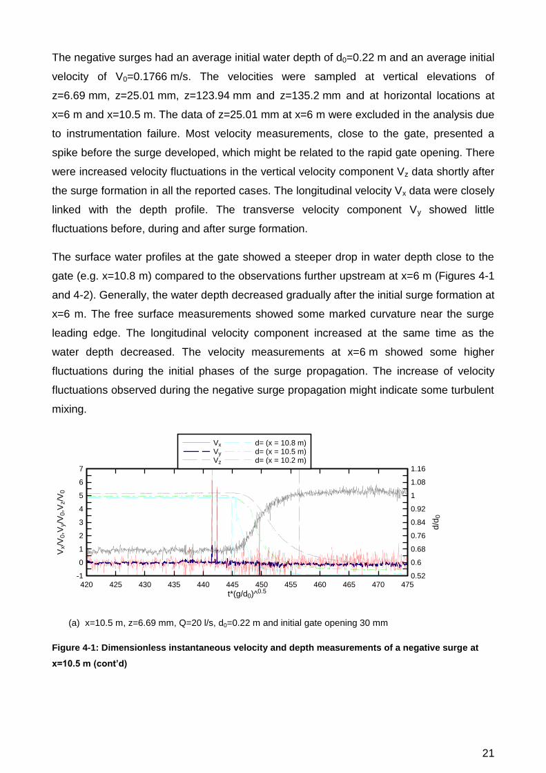
The negative surges had an average initial water depth of d0=0.22 m and an average initial

velocity of V0=0.1766 m/s. The velocities were sampled at vertical elevations of

z=6.69 mm, z=25.01 mm, z=123.94 mm and z=135.2 mm and at horizontal locations at

x=6 m and x=10.5 m. The data of z=25.01 mm at x=6 m were excluded in the analysis due

to instrumentation failure. Most velocity measurements, close to the gate, presented a

spike before the surge developed, which might be related to the rapid gate opening. There

were increased velocity fluctuations in the vertical velocity component Vz data shortly after

the surge formation in all the reported cases. The longitudinal velocity Vx data were closely

linked with the depth profile. The transverse velocity component Vy showed little

fluctuations before, during and after surge formation.

The surface water profiles at the gate showed a steeper drop in water depth close to the

gate (e.g. x=10.8 m) compared to the observations further upstream at x=6 m (Figures 4-1

and 4-2). Generally, the water depth decreased gradually after the initial surge formation at

x=6 m. The free surface measurements showed some marked curvature near the surge

leading edge. The longitudinal velocity component increased at the same time as the

water depth decreased. The velocity measurements at x=6 m showed some higher

fluctuations during the initial phases of the surge propagation. The increase of velocity

fluctuations observed during the negative surge propagation might indicate some turbulent

mixing.

(a) x=10.5 m, z=6.69 mm, Q=20 l/s, d0=0.22 m and initial gate opening 30 mm

Figure 4-1: Dimensionless instantaneous velocity and depth measurements of a negative surge at

x=10.5 m (cont’d)

t*(g/d0)^0.5

Vx/V

0,V

y/V

0,V

z/V

0

d/d

0

420 425 430 435 440 445 450 455 460 465 470 475-1 0.52

0 0.6

1 0.68

2 0.76

3 0.84

4 0.92

5 1

6 1.08

7 1.16

Vx

Vy

Vz

d= (x = 10.8 m)d= (x = 10.5 m)d= (x = 10.2 m)

22

(b) x=10.5 m, z=25.01 mm, Q=20 l/s, d0=0.22 m and initial gate opening 30 mm

(c) x=10.5 m, z=123.94 mm, Q=20 l/s, d0=0.22 m and initial gate opening 30 mm

(d) x=10.5 m, z=135.2 mm , Q=20 l/s, d0=0.22 m and initial gate opening 30 mm


x=10.5 m

t*(g/d0)^0.5

Vx/V

0,V

y/V

0,V

z/V

0

d/d

0

390 395 400 405 410 415 420 425 430 435 440 445-1 0.52

0 0.6

1 0.68

2 0.76

3 0.84

4 0.92

5 1

6 1.08

7 1.16

t*(g/d0)^0.5

Vx/V

0,V

y/V

0,V

z/V

0

d/d

0

360 362 364 366 368 370 372 374 376 378 380 382 384 386 388 390 392 394 396 398 400-1 0.52

0 0.6

1 0.68

2 0.76

3 0.84

4 0.92

5 1

6 1.08

7 1.16

t*(g/d0)^0.5

Vx/V

0,V

y/V

0,V

z/V

0

d/d

0

295 296 297 298 299 300 301 302 303 304 305 306 307 308 309 310 311 312 313 314 315-1 0.52

0 0.6

1 0.68

2 0.76

3 0.84

4 0.92

5 1

6 1.08

7 1.16

23

(a) x=6 m, z=6.69 mm, Q=20 l/s, d0=0.22 m and initial gate opening 30 mm

(b) x=6 m, z=123.94 mm, Q=20 l/s, d0=0.22 m and initial gate opening 30 mm

(c) x=6 m, z=135.2 mm, Q=20 l/s, d0=0.22 m and initial gate opening 30 mm


x=6 m

t*(g/d0)^0.5

Vx/V

0,V

y/V

0,V

z/V

0

d/d

0

400 405 410 415 420 425 430 435 440 445 450 455-1 0.52

0 0.6

1 0.68

2 0.76

3 0.84

4 0.92

5 1

6 1.08

7 1.16

Vx

Vy

Vz

d= (x = 6.2 m)d= (x = 6.0 m)d= (x = 5.6 m)

t*(g/d0)^0.5

Vx/V

0,V

y/V

0,V

z/V

0

d/d

0

435 440 445 450 455 460 465 470 475 480 485 490-1 0.52

0 0.6

1 0.68

2 0.76

3 0.84

4 0.92

5 1

6 1.08

7 1.16

t*(g/d0)^0.5

Vx/V

0,V

y/V

0,V

z/V

0

d/d

0

415 420 425 430 435 440 445 450 455 460 465 470-1 0.52

0 0.6

1 0.68

2 0.76

3 0.84

4 0.92

5 1

6 1.08

7 1.16

24

4.1.2 Positive surge

The positive surges had an average initial water depth of d0=0.064 m and an average

initial velocity of V0=0.625 m/s. Typical instantaneous free-surface profiles and ADV

velocity recordings for the positive surges are presented in Figures 4-3 and 4-4. The data

of z=25.01 mm at x=6 m were excluded in the analysis due to instrumentation failure.

The figures are presented in instantaneous dimensionless flow depth d/do as a function of

dimensionless time from gate closure 0/ dgt , where do is the initial water depth at

x=6 m and x=10.5 m respectively. The acoustic displacement meter output was a function

of the strength of the acoustic signal reflected by the free-surface. When the free-surface

was not horizontal, some erroneous points were recorded. These were relatively isolated

and easily identified. Overall the data showed a gradual evolution of the positive surge

shape as it propagated upstream (e.g. from x=10.8 m to x=6 m) (Figure 4-3). The data

suggested a slight reduction in surge height with increasing distance from the downstream

gate. Figure 4-3(a) shows the positive surge propagation at x=6 m. A decrease in the Vx

velocity component can be observed in the initial phase of the positive surge. The Vy and

Vz velocity components did not show any major change in pattern between the steady

state phase and the propagation of the positive surge. Significant Vz spikes were observed

near the gate as seen in Figure 4-4 (b) and (c).


Figure 4-3: Dimensionless instantaneous velocity and depth measurements of a positive surge at

x=6 m

t*(g/d0)^0.5

Vx/

V0,V

y/V

0,V

z/V

0

d/d

0

900 905 910 915 920 925 930 935 940 945 950 955-0.5 0.9

-0.3 1.02

-0.1 1.14

0.1 1.26

0.3 1.38

0.5 1.5

0.7 1.62

0.9 1.74

1.1 1.86

1.3 1.98

1.5 2.1

Vx

Vy

Vz

d= (x = 6.2 m)d= (x = 6.0 m)d= (x = 5.6 m)

25


(b) x=10.5 m, z=123.94 mm , Q=20 l/s, d0=0.064 m

Figure 4-4: Dimensionless instantaneous velocity and depth measurements of a positive surge at

x=10.5 m

4.2 Video analysis results

Video imagery was used to record the surface profile of the positive and negative surges.

The surface profiles of the propagation of the positive and negative surges were analysed

at 6 m and at 10.8 m. The video imagery was analysed frame by frame, with 25 frames per

second from the first opening or closing of the gate. A summary of the experimental flow

conditions is provided in Table 4.2. Photographs of a positive and negative surge are

shown in Figure 4-5.

t*(g/d0)^0.5

Vx/V

0,V

y/V

0,V

z/V

0

d/d

0

850 855 860 865 870 875 880 885 890 895 900 905-0.5 0.9

-0.3 1.02

-0.1 1.14

0.1 1.26

0.3 1.38

0.5 1.5

0.7 1.62

0.9 1.74

1.1 1.86

1.3 1.98

1.5 2.1

Vx

Vy

Vz

d= (x = 10.8 m)d= (x = 10.5 m)d= (x = 10.2 m)

t*(g/d0)^0.5

Vx/V

0,V

y/V

0,V

z/V

0

d/d

0

790 795 800 805 810 815 820 825 830 835 840 845-0.5 0.9

-0.3 1.02

-0.1 1.14

0.1 1.26

0.3 1.38

0.5 1.5

0.7 1.62

0.9 1.74

1.1 1.86

1.3 1.98

1.5 2.1

26

(a) (b)

Figure 4-5: Photos of (a) positive and (b) negative surge near the gate at (11.2 m< x <10.48 m)

Table 4-2: Experimental flow conditions for water surface measurements using video analysis

Discharge (Q) (l/s) Gate opening (mm) Type of surge V0 (m/s) d0 (m) Location

(x) (m)

20

30 Negative 0.167 0.24 6, 10.5

Positive 0.667 0.06 6, 10.5

50 Negative 0.400 0.10 6, 10.5

Positive 0.667 0.06 6, 10.5

30

40 Negative 0.231 0.26 6, 10.5

Positive 0.750 0.08 6, 10.5

50 Negative 0.273 0.22 6, 10.5

Positive 0.857 0.07 6, 10.5


The results are illustrated in dimensionless water depth and dimensionless distance x

within the recorded frame. Each curve represents the time step for one frame, with a

recording speed of 25 frames per second. The results are presented in Figure 4-6 at

x=10.5 m and Figure 4-7 at x=6 m. The results close to the gate at x=10.5 m showed, that

the flow pattern is very similar regardless of the initial gate opening and discharge. Due to

the gate opening there is an initial rise at the beginning of the surge with a slow and steady

fall of the water surface elevation. The water depth decreases faster at the beginning of

the surge compared to the later stages of the surge. At 6 m the water surface has no

curvature anymore. It was observed that the negative surge with Q= 20 l/s and a 50 mm

gate opening showed the lowest variation in water depth between each frame. A slight

curvature was observed at the dimensionless distance x’/d0=1.25 in the results of the

negative surge at x=6 m with a 30 l/s discharge and a 50 mm gate opening. Overall, the

video data provided a good illustration of the water depth profile, showing the propagation

of the negative surge as a gradual lowering of the water surface.

27

(a) Q=20 l/s and 30 mm gate opening

(b) Q=20 l/s and 50 mm gate opening


Figure 4-6: Dimensionless video data for the negative surge immediately u/s of the gate 10.5 m, with

x’=0 corresponding to x=11.2 m (cont’d)

x'/d0

d/d

0

0 0.25 0.5 0.75 1 1.25 1.5 1.75 2 2.250.10.20.30.40.50.60.70.80.9

11.11.2

123

456

789

101112

131415

161718

192021

222324

2526

x'/d0

d/d

0

0 0.5 1 1.5 2 2.5 3 3.5 4 4.50.4

0.5

0.6

0.7

0.8

0.9

1

123

456

789

101112

131415

161718

19

x'/d0

d/d

0

0 0.25 0.5 0.75 1 1.25 1.5 1.75 2 2.25 2.5 2.750.30.40.50.60.70.80.9

11.11.21.31.4

123

456

789

101112

131415

161718

192021

222324

2526

28

(d) Q=30 l/s and 50 mm gate opening

Figure 4-6: Dimensionless video data for the negative surge immediately u/s of the gate 10.5 m, with

x’=0 corresponding to x=11.2 m



Figure 4-7: Dimensionless video data for the negative surge at 6 m, with x’=0 corresponding to x=6.3

m (cont’d)

x'/d0

d/d

0

0 0.25 0.5 0.75 1 1.25 1.5 1.75 2 2.25 2.5 2.750.2

0.4

0.6

0.8

1

1.2

1.4

123

456

789

101112

131415

1617

x'/d0

d/d

0

0 0.5 1 1.5 2 2.5 3 3.50.9

0.925

0.95

0.975

1

1.025

1.05

1.075

1.1 1 5 10 15 20 25 30 35 40 45 50

x'/d0

d/d

0

0 0.25 0.5 0.75 1 1.25 1.5 1.75 2 2.25 2.5 2.750.92

0.94

0.96

0.98

1

1.02

1.04

1.06

1.08 1 5 10 15 20

29

(c) Q=30 l/s and 40 mm gate opening


Figure 4-7: Dimensionless video data for the negative surge at 6 m, with x’=0 corresponding to x= 6.3

m


The results are illustrated in dimensionless water depth and dimensionless distance x

within the recorded frame. The first frame corresponded to the start of the gate opening.

The results are presented for the positive surge in Figure 4-8 at x=10.5 m and Figure 4-9

at x=6 m. The curves are plotted for each frame with a 25 frames per second camera

speed. The positive surge video analysis showed that there is a difference in surge

propagation and water depth with different discharge conditions and initial gate openings.

The results of the experiments performed with a discharge of 20 l/s and a gate opening of

50 mm showed that the surge propagates slower than the surge in the other experiments.

x'/d0

d/d

0

0 0.25 0.5 0.75 1 1.25 1.5 1.75 2 2.25 2.50.86

0.88

0.9

0.92

0.94

0.96

0.98

1

1.02

1.04

1 5 10 15 20 25 30 35 40 45 50

x'/d0

d/d

0

0 0.3 0.6 0.9 1.2 1.5 1.8 2.1 2.4 2.70.88

0.90.920.940.960.98

11.021.041.061.08

1.1

1 5 10 15 20 25 30 35 40 45

30

The increase in water depth can be best observed at the beginning of the surge formation.

After a quick initial rise in water depth the water surface rose gradually until it came to a

steady state.

The surface profiles of the positive surge were similar for both observed locations, x=10.5

m and x=6 m. The water depth at x=6 m showed the steady propagation of the surge front

with a rise of approximately 0.2 d/d0 between the initial conditions and the water depth at

frame 32 (∆t=1.28 s).



Figure 4-8: Dimensionless video data for the positive surge at 10.5 m, with x’=0 corresponding to

x=11.2 m (cont’d)

x'/d0

d/d

0

0.5 1 1.5 2 2.5 3 3.5 4 4.5 5 5.5 6 6.5 70.85

0.95

1.05

1.15

1.25

1.35

1.45

1.55

123

456

789

101112

131415

161718

192021

222324

252627

2829

x'/d0

d/d

0

0.5 1 1.5 2 2.5 3 3.5 4 4.5 5 5.5 6 6.5 70.8

0.9

1

1.1

1.2

1.3

1.4

1.5

123

456

789

101112

131415

161718

192021

222324

252627

282930

313233

31



Figure 4-8: Dimensionless video data for the positive surge at x= 10.5 m, with x’=0 corresponding to

x=11.2 m


Figure 4-9: Dimensionless video data for the positive surge at x= 6 m, with x’=0 corresponding to

x=6.9 m (cont’d)

x'/d0

d/d

0

0.5 1 1.5 2 2.5 3 3.5 4 4.5 5 5.5 6 6.50.95

1.05

1.15

1.25

1.35

1.45

1.55

1.65

123

456

789

101112

131415

161718

192021

222324

252627

2829

x'/d0

d/d

0

0 0.5 1 1.5 2 2.5 3 3.5 4 4.5 50.75

0.8

0.85

0.9

0.95

1

1.05

1.1

1.15

1.2

1.25

123

456

789

101112

131415

161718

192021

222324

252627

x'/d0

d/d

0

0 0.5 1 1.5 2 2.5 3 3.5 4 4.5 50.75

0.85

0.95

1.05

1.15

1.25 123

456

789

101112

131415

161718

192021

222324

252627

282930

3132

32




Figure 4-9: Dimensionless video data for the positive surge at x=6 m, with x’=0 corresponding to

x=6.9 m

x'/d0

d/d

0

0 0.6 1.2 1.8 2.4 3 3.6 4.2 4.8 5.40.85

0.95

1.05

1.15

1.25

1.35

1.45

1.55

123

456

789

101112

131415

161718

192021

222324

252627

282930

3132

x'/d0

d/d

0

0 0.5 1 1.5 2 2.5 3 3.5 4 4.5 5 5.5 6 6.5 71

1.051.1

1.151.2

1.251.3

1.351.4

1.451.5

1.55

123

456

789

101112

131415

161718

192021

222324

252627

282930

313233

343536

373839

404142

434445

464748

4950

x'/d0

d/d

0

0 0.5 1 1.5 2 2.5 3 3.5 4 4.5 5 5.5 6 6.5 70.95

1

1.05

1.1

1.15

1.2

1.25

1.3

123

456

789

101112

131415

161718

192021

222324

252627

282930

313233

343536

373839

404142

434445

464748

4950

33

4.3 Ensemble-average results

In a turbulent unsteady flow, the analysis of the time average data is not meaningful,

because the hydrodynamic shock and the short-term fluctuation must be analysed

independently. Therefore, the experiments were repeated several times to obtain an

ensemble average of the instantaneous data. For both negative and positive surges the

free-surface properties and velocity characteristics were systematically investigated at

x=10.5 m and x=6 m. A total of 25 runs were conducted for the two layouts and four

vertical elevations of the ADV. The data was analysed and scattered runs were eliminated.

The remaining runs, typically 20 runs or greater, were ensemble-averaged.


Figures 4-10 shows some typical synchronised dimensionless data of the instantaneous

water depth, velocities, as well as the median water depth and median velocities for the

negative surge. An ensemble-median of each instantaneous velocity component was

produced for each vertical elevation of the ADV measurements. All the negative surge

data were synchronised based on the characteristic time t3 which is further illustrated in

Appendix B. The instantaneous depth data was plotted for every run of the 25 runs and the

first derivative was calculated. The data was then filtered using a 0-1 Hz band pass. The

error in the data synchronisation process was estimated at up to 1%.

Figures 4-11(a) presents some typical results of the ensemble averaged median water

depth dMedian, the differences between the 3rd and 4th quartiles (d75- d25) and 90% and 10%

percentiles (d90-d10) and the maximum height between the minimum and maximum water

depth (dmax-dmin) at x=6 m and z=6.69 mm for the negative surge.

Figures 4-11(b) presents the ensemble averaged median water depth dMedian, the

differences between the 3rd and 4th quartiles (d75- d25) and 90% and 10% percentiles (d90-

d10) and the maximum height between the minimum and maximum water depth (dmax-dmin)

at x=10.5 m z=6.69 mm for the negative surge. The full data sets of the ensemble average

water depth for all vertical ADV locations at x=6 m and x=10.5 m are reported in Appendix

B.

Some typical experimental results are shown in Figure 4-12 and Figure 4-13 in terms of

the ensemble-averaged velocity components as a function of dimensionless time.

34

Each graph includes the ensemble-averaged median velocity component (Vx, Vy, or Vz),

the maximum velocity between the minimum and the maximum (Vmax- Vmin), the

differences between the 3rd and 4th quartiles (V75-V25), the 90% and 10% percentiles(V90-

V10), and the ensemble-averaged median water depth dMedian. The full data set is

presented in Appendix B.

The ensemble-averaged median water depth showed a steeper curvature for the data

recorded at the gate at x=10.5 m compared to the data further upstream at x=6 m. The

finding was consistent with the results of the instantaneous data presented in section 4.1.

The inflection point of the median water depth and the inflection point for the longitudinal

velocity Vx occurred approximately at the same time during the passage of the surge. The

fluctuations of the longitudinal velocity Vx seemed to slightly increase near the inflection

point of the negative surge, especially near the gate at x=10.5 m. It was also observed

further upstream, but the fluctuations were smaller. The Vy velocities were very scattered

at x=6 m and z=6.69 mm. However, the median velocities showed little fluctuations. The Vz

velocities showed a slight increase in minimum and maximum velocity fluctuations at the

beginning of the surge. Overall, the median Vz velocities did not show large variations. The

median dimensionless velocities for Vz and Vy were of similar magnitude. To date there is

no previous data available to compare the results.

(a) time variation of median water depth dMedian at x=10.5 m

(c) time variation of median velocity in the longitudinal direction VxMedian at x=6 m

Figure 4-10: Instantaneous and median data for all 25 runs for the negative surge at z=6.69 mm

(cont’d)

t*(g/d0)^0.5

d/d 0

, d/d

Med

ian

60 61 62 63 64 65 66 67 68 69 70 71 72 73 74 75 76 77 78 79 800.5

0.6

0.7

0.8

0.9

1

1.1dMedian

t*(g/d0)^0.5

Vx/

V0,

VxM

edia

n/V

0

85 87.5 90 92.5 95 97.5 100 102.5 105 107.5 110 112.5 115 117.5 1200

0.4

0.8

1.2

1.6

2

2.4

2.8

3.2

3.6

4

VxMedian

35

(c) time variation of median velocity in the cross-sectional direction VyMedian at x=6 m

(d) time variation of median velocity in the vertical direction VzMedian at x=6 m

Figure 4-10: Instantaneous and median data for all 25 runs for the negative surge at z=6.69 mm

(a) x=6 m and z=6.69 mm

Figure 4-11: Dimensionless ensemble-average median water depth dMedian, difference between 3rd

and 4th quartiles (d75-d25) and 90% and 10% percentiles (d90-d10), and range of maximum to minimum

water depth (dmax-dmin) (cont’d)

t*(g/d0)^0.5

Vy/

V0,

VyM

edia

n/V

0

85 87.5 90 92.5 95 97.5 100 102.5 105 107.5 110 112.5 115 117.5 120-0.5

-0.4

-0.3

-0.2

-0.1

0

0.1

0.2

0.3

0.4

VyMedian

t*(g/d0)^0.5

Vz/

V0,

VzM

edia

n/V

0

85 87.5 90 92.5 95 97.5 100 102.5 105 107.5 110 112.5 115 117.5 120-2

-1.6

-1.2

-0.8

-0.4

0

0.4

0.8

1.2

1.6

2

VzMedian

t*(g/d0)0.5

d Med

ian/

d 0

d 75-

d 25/

d 0, d

90-d

10/d

0, d

max

-dm

in/d

0

85 87.5 90 92.5 95 97.5 100 102.5 105 107.5 110 112.5 115 117.5 1200.55 0

0.6 0.06

0.65 0.12

0.7 0.18

0.75 0.24

0.8 0.3

0.85 0.36

0.9 0.42

0.95 0.48

1 0.54

1.05 0.6

1.1 0.66

dMedian

dmax-dmin

d90-d10

d75-d25

36

(b) x=10.5 m and z=6.69 mm



water depth (dmax-dmin)

(a) Vx

(b) Vy

Figure 4-12: Dimensionless ensemble-average median velocity VMedian, difference between 3rd and

4th quartiles (V75- V25) and 90% and 10% percentiles (V90- V10), and range of maximum to minimum

water depth (Vmax- Vmin) at x=6 m and z=6.69 mm (cont’d)

t*(g/d0)0.5

d Med

ian/

d 0

d 75-

d 25/

d 0, d

90-d

10/d

0, d

max

-dm

in/d

0

65 66 67 68 69 70 71 72 73 74 750.55 0

0.6 0.06

0.65 0.12

0.7 0.18

0.75 0.24

0.8 0.3

0.85 0.36

0.9 0.42

0.95 0.48

1 0.54

1.05 0.6

1.1 0.66

dMedian

dmax-dmin

d90-d10

d75-d25

t*(g/d0)0.5

d Med

ian/

d 0

VxM

edia

n/V

0, V

xmax

-Vxm

in/V

0, V

x75-

Vx2

5/V

0, V

x90-

Vx1

0/V

0,

85 87.5 90 92.5 95 97.5 100 102.5 105 107.5 110 112.5 115 117.5 1200.55 -1.6

0.6 -0.8

0.65 0

0.7 0.8

0.75 1.6

0.8 2.4

0.85 3.2

0.9 4

0.95 4.8

1 5.6

1.05 6.4

1.1 7.2

dMedian

VxMedian

Vxmax-Vxmin

Vx90-Vx10

Vx75-Vx25

t*(g/d0)0.5

dM

edia

n/d

0

VyM

edia

n/V

0,

Vym

ax-

Vym

in/V

0,

Vy7

5-V

y25/V

0,

Vy9

0-V

y10/V

0,

85 87.5 90 92.5 95 97.5 100 102.5 105 107.5 110 112.5 115 117.5 1200.55 -1.6

0.6 -0.8

0.65 0

0.7 0.8

0.75 1.6

0.8 2.4

0.85 3.2

0.9 4

0.95 4.8

1 5.6

1.05 6.4

1.1 7.2

dMedian

VyMedian

Vymax-Vymin

Vy90-Vy10

Vy75-Vy25

37

(c) Vz



water depth (Vmax- Vmin) at x=6 m and z=6.69 mm.

(a) Vx

(b) Vy

Figure 4-13: Dimensionless ensemble-average median velocity VMedian, difference between 3rd

and 4th quartiles (V75- V25) and 90% and 10% percentiles (Vz90- Vz10), and range of maximum to

minimum water depth (Vmax- Vmin) at x=10.5 m and z=6.69 mm.

t*(g/d0)0.5

dM

edia

n/d

0

VzM

edia

n/V

0,

Vzm

ax-

Vzm

in/V

0,

Vz7

5-V

z25/V

0,

Vz9

0-V

z10/V

0,

85 87.5 90 92.5 95 97.5 100 102.5 105 107.5 110 112.5 115 117.5 1200.55 -1.6

0.6 -0.8

0.65 0

0.7 0.8

0.75 1.6

0.8 2.4

0.85 3.2

0.9 4

0.95 4.8

1 5.6

1.05 6.4

1.1 7.2

dMedian

VzMedian

Vzmax-Vzmin

Vz90-Vz10

Vz75-Vz25

t*(g/d0)0.5

d Med

ian/

d 0

VxM

edia

n/V

0, V

xmax

-Vxm

in/V

0, V

x75-

Vx2

5/V

0, V

x90-

Vx1

0/V

0,

65 66 67 68 69 70 71 72 73 74 750.55 -1.6

0.6 -0.8

0.65 0

0.7 0.8

0.75 1.6

0.8 2.4

0.85 3.2

0.9 4

0.95 4.8

1 5.6

1.05 6.4

1.1 7.2

dMedian

VxMedian

Vxmax-Vxmin

Vx90-Vx10

Vx75-Vx25

t*(g/d0)0.5

d Med

ian/

d 0

VyM

edia

n/V

0, V

ymax

-Vym

in/V

0, V

y75-

Vy2

5/V

0, V

y90-

Vy1

0/V

0,

65 66 67 68 69 70 71 72 73 74 750.55 -1.6

0.6 -0.8

0.65 0

0.7 0.8

0.75 1.6

0.8 2.4

0.85 3.2

0.9 4

0.95 4.8

1 5.6

1.05 6.4

1.1 7.2

dMedian

VyMedian

Vymax-Vymin

Vy90-Vy10

Vy75-Vy25

38

(c) Vz


4th quartiles (V75- V25) and 90% and 10% percentiles (Vz90- Vz10), and range of maximum to minimum

water depth (Vmax- Vmin) at x=10.5 m and z=6.69 mm.


Figure 4-14 shows the dimensionless data of the synchronised instantaneous water depth,

velocities, as well as the median water depth and median velocities for the positive surge.

An ensemble-median of each instantaneous velocity component was produced for each

vertical elevation of the ADV measurements. All the positive surge data were synchronised

based on the characteristic time t3, which is further illustrated in Appendix C. The

characteristic points of the positive surge were identified in previous studies by Docherty

and Chanson (2010). The estimated error in the data synchronisation process was

estimated at up to 2%.

Figures 4-15 presents the ensemble averaged median water depth dMedian, the differences

between the 3rd and 4th quartiles (d75- d25) and 90% and 10% percentiles (d90-d10) and the

maximum height between the minimum and maximum water depth (dmax-dmin) for the

positive surge. The full data set of the ensemble-averaged velocities for all vertical ADV

locations and the two longitudinal locations x=10.5 m and x=6 m are presented in

Appendix C.

Some typical experimental results are shown in Figure 4-16 and Figure 4-17 in terms of

the ensemble-averaged velocity components as a function of dimensionless time.

t*(g/d0)0.5

dM

edia

n/d

0

VzM

edia

n/V

0,

Vzm

ax-

Vzm

in/V

0,

Vz7

5-V

z25/V

0,

Vz9

0-V

z10/V

0,

65 66 67 68 69 70 71 72 73 74 750.55 -1.6

0.6 -0.8

0.65 0

0.7 0.8

0.75 1.6

0.8 2.4

0.85 3.2

0.9 4

0.95 4.8

1 5.6

1.05 6.4

1.1 7.2

dMedian

VzMedian

Vzmax-Vzmin

Vz90-Vz10

Vz75-Vz25

39

Each graph includes the ensemble-averaged median velocity component (Vx, Vy, or Vz),

the maximum velocity between the minimum and the maximum (Vmax- Vmin), the

differences between the 3rd and 4th quartiles (V75-V25), the 90% and 10% percentiles(V90-

V10), and the ensemble-averaged median water depth dMedian. The full data set is

presented in Appendix C.

The maximum fluctuation of the water depth occurred at the same time as the maximum

fluctuations of the vertical velocities Vx. The maximum fluctuation of the longitudinal

velocity Vx occurred in the surge front passage, as seen by the large values of the

differences between the 90th and the 10th percentile.

The average vertical velocity component was positive during the surge front passage.

There was little fluctuation of the Vy velocities during the surge propagation. Since the

surge was produced using a relatively small discharge the fluctuations of the velocities are

less profound then observed in previous studies, such as Docherty and Chanson (2010)

and Koch and Chanson (2009). However, the results confirmed the findings of

characteristic trends in positive surges of previous studies by Koch and Chanson (2009)

and Docherty and Chanson (2010).

(a) time variation of median water depth dMedian

Figure 4-14: Instantaneous and median data for the positive surge at x=6m and z=6.69 mm (cont’d)

t*(g/d0)^0.5

d/d

0,

dM

edia

n/d

0

120 123 126 129 132 135 138 141 144 147 150 153 156 159 162 165 168 171 174 177 1800.9

1

1.1

1.2

1.3

1.4

1.5

1.6

1.7

1.8

dmedian

40

(b) time variation of median velocity in the longitudinal direction VxMedian

(c) time variation of median velocity in the cross-sectional direction VyMedian

(d) time variation of median velocity in the vertical direction VzMedian.

Figure 4-14: Instantaneous and median data for the positive surge at x=6m and z=6.69 mm

t*(g/d0)^0.5

Vx/

V0,

VxM

ed

ian/V

0

120 123 126 129 132 135 138 141 144 147 150 153 156 159 162 165 168 171 174 177 180-0.15

0

0.15

0.3

0.45

0.6

0.75

0.9

1.05

1.2

1.35

1.5

VxMedian

t*(g/d0)^0.5

Vy/

V0,

VyM

ed

ian/V

0

120 123 126 129 132 135 138 141 144 147 150 153 156 159 162 165 168 171 174 177 180-0.2

-0.16

-0.12

-0.08

-0.04

0

0.04

0.08

0.12

0.16

0.2

VyMedian

t*(g/d0)^0.5

Vz/

V0,

VzM

edia

n/V

0

120 123 126 129 132 135 138 141 144 147 150 153 156 159 162 165 168 171 174 177 180-0.7

-0.5

-0.3

-0.1

0.1

0.3

0.5

0.7

0.9

1.1 VzMedian

41

(a) x=6 m and z=6.69 mm

(a) x=10.5 m and z=6.69 mm



water depth (dmax-dmin)

t*(g/d0)0.5

dM

ed

ian/d

0

d7

5-d

25/d

0,

d9

0-d

10/d

0,

dm

ax-d

min

/d0

230 240 250 260 270 280 290 300 310 320 3300.9 0

1 0.08

1.1 0.16

1.2 0.24

1.3 0.32

1.4 0.4

1.5 0.48

1.6 0.56

1.7 0.64

1.8 0.72

dMedian

dmax-dmin

d90-d10

d75-d25

t*(g/d0)0.5

dM

edia

n/d

0

d75-d

25/d

0,

d90-d

10/d

0,

dm

ax-d

min

/d0

120 123 126 129 132 135 138 141 144 147 150 153 156 159 162 165 168 171 174 177 1800.9 0

1 0.08

1.1 0.16

1.2 0.24

1.3 0.32

1.4 0.4

1.5 0.48

1.6 0.56

1.7 0.64

1.8 0.72

dMedian

dmax-dmin

d90-d10

d75-d25

42

(a) Vx

(b) Vy

(c) Vz



water depth (Vmax- Vmin) at x=6 m and z=6.69 mm.

t*(g/d0)0.5

dM

ed

ian/d

0

VxM

ed

ian/V

0,

Vxm

ax-

Vxm

in/V

0,

Vx7

5-V

x25/V

0,

Vx9

0-V

x10/V

0,

230 240 250 260 270 280 290 300 310 320 3300.9 -0.15

1 0.15

1.1 0.45

1.2 0.75

1.3 1.05

1.4 1.35

1.5 1.65

1.6 1.95

1.7 2.25

1.8 2.55

dMedian

VxMedian

Vxmax-Vxmin

Vx90-Vx10

Vx75-Vx25

t*(g/d0)0.5

dM

ed

ian/d

0

VyM

ed

ian/V

0,

Vym

ax-

Vym

in/V

0,

Vy7

5-V

y25/V

0,

Vy9

0-V

y10/V

0,

230 240 250 260 270 280 290 300 310 320 3300.9 -0.15

1 0.15

1.1 0.45

1.2 0.75

1.3 1.05

1.4 1.35

1.5 1.65

1.6 1.95

1.7 2.25

1.8 2.55

dMedian

VyMedian

Vymax-Vymin

Vy90-Vy10

Vy75-Vy25

t*(g/d0)0.5

dM

ed

ian/d

0

VzM

ed

ian/V

0,

Vzm

ax-

Vzm

in/V

0,

Vz7

5-V

z25/V

0,

Vz9

0-V

z10/V

0,

230 240 250 260 270 280 290 300 310 320 3300.9 -0.15

1 0.15

1.1 0.45

1.2 0.75

1.3 1.05

1.4 1.35

1.5 1.65

1.6 1.95

1.7 2.25

1.8 2.55

dMedian

VzMedian

Vzmax-Vzmin

Vz90-Vz10

Vz75-Vz25

43

(a) Vx

(b) Vy

(c) Vz


4th quartiles (V75- V25) and 90% and 10% percentiles (Vz90- Vz10), and range of maximum to minimum

water depth (Vmax- Vmin) at x=10.5 m and z=6.69 mm.

t*(g/d0)0.5

dM

ed

ian/d

0

VxM

ed

ian/V

0,

Vxm

ax-

Vxm

in/V

0,

Vx7

5-V

x25/V

0,

Vx9

0-V

x10/V

0,

120 123 126 129 132 135 138 141 144 147 150 153 156 159 162 165 168 171 174 177 1800.9 -0.15

1 0.15

1.1 0.45

1.2 0.75

1.3 1.05

1.4 1.35

1.5 1.65

1.6 1.95

1.7 2.25

1.8 2.55

dMedian

VxMedian

Vxmax-Vxmin

Vx90-Vx10

Vx75-Vx25

t*(g/d0)0.5

dM

ed

ian/d

0

VyM

ed

ian/V

0,

Vym

ax-

Vym

in/V

0,

Vy7

5-V

y25/V

0,

Vy9

0-V

y10/V

0,

120 123 126 129 132 135 138 141 144 147 150 153 156 159 162 165 168 171 174 177 1800.9 -0.15

1 0.15

1.1 0.45

1.2 0.75

1.3 1.05

1.4 1.35

1.5 1.65

1.6 1.95

1.7 2.25

1.8 2.55

dMedian

VyMedian

Vymax-Vymin

Vy90-Vy10

Vy75-Vy25

t*(g/d0)0.5

dM

ed

ian/d

0

VzM

ed

ian/V

0,

Vzm

ax-

Vzm

in/V

0,

Vz7

5-V

z25/V

0,

Vz9

0-V

z10/V

0,

120 123 126 129 132 135 138 141 144 147 150 153 156 159 162 165 168 171 174 177 1800.9 -0.15

1 0.15

1.1 0.45

1.2 0.75

1.3 1.05

1.4 1.35

1.5 1.65

1.6 1.95

1.7 2.25

1.8 2.55

dMedian

VzMedian

Vzmax-Vzmin

Vz90-Vz10

Vz75-Vz25

44

4.4 Discussion

The celerity of the negative surge was measured from the video and acoustic

displacement meter data. Figure 4-18 illustrates the results in dimensionless terms with a

dotted line showing the location of the gate. Figure 4-18(a) shows the data for one set of

flow conditions. Figure 4-18(b) shows the dimensionless celerity data with x/L, where L

refers to the channel length of 12 m. This dimensionless presentation enabled the

comparison of different flow conditions. The flow conditions are summarised in Table 4-3.

The full data sets are presented in Appendix E.

The experimental results showed two distinct phases. Very close to the gate, and

immediately after gate closure, the negative surge formation was associated with some

local dissipative process illustrated in Appendix A. During this formation phase, the celerity

of the negative surge leading edge increased with time. Within the experimental flow

conditions (Table 4-3), the present data sets suggested that the acceleration phase took

place within 1 m from the gate. After the acceleration/formation phase, the negative surge

propagated upstream in a more gradual manner. During this gradually-varied phase, the

surge leading edge was very flat and barely perceptible by human eye, and its celerity

tended to decrease slowly with increasing distance from the gate as shown in Figure 4-

18(a) for x/do < 40. The data tended to imply some effect of flow resistance in manner

possibly opposite to that predicted by Henderson (1966, pp. 297-299). At x=6 m, the

dimensionless negative surge celerity (U+Vo)/sqrt(g do) ranged from 0.3 up to 1.0

depending upon the initial steady flow conditions (Table 4-3, 5th column).

For comparison, the analytical solution of the Saint-Venant equations for a simple wave

predicts that the leading edge of the negative surge propagates with a constant

dimensionless celerity (U+Vo)/sqrt(g do)=1. Lauber and Hager (1998) performed

experiments in a horizontal rectangular channel initially at rest (Vo=0) with a 3.5 m long

reservoir. They observed U/sqrt(g do) =sqrt(2) =1.41. Tan and Chu (2009) re-analysed the

data of Lauber and Hager, and their computational data matched the experimental

observations yielding U/sqrt(g do)=1. The present results (Figure 4-18, Table 4-3 &

Appendix E) suggest that neither the Saint-Venant equations solution nor previous findings

are applicable herein. While the negative surge formation might be affected by the gate

opening mechanism, the gradually-varied phase associated with a slow deceleration of the

negative surge leading edge was likely linked with the initial flow conditions and flow

resistance. The present findings suggested that further studies are required to assess the

effect of initial flow conditions and flow resistance on the propagation of negative surges.

45

Table 4-3: Flow conditions and celerity measurement

Q (l/s) Gate opening h (mm)

V0 at x=6m m/s

d0 at x=6 m m

(U+Vo)/sqrt(g do) at x=6

Remark

20 30 0.167 0.23 1.0 0.7-1.17 for 5.6 < x < 8.55 m

20 50 0.4 0.1 0.66

30 40 0.231 0.26 0.30

30 50 0.273 0.22

0.52

(a) Dimensionless celerity (U+Vo)/(g do)1/2

as function of longitudinal distance x/do for Q=0.020 m3/s and

h=30 mm

(b) Dimensionless celerity (U+Vo)/(g do)1/2

as function of longitudinal distance x/L (L=12 m)

Figure 4-18: Celerity of negative surges

x/d0

(U+

V0)/

(g*d

0)1

/2

21 24 27 30 33 36 39 42 45 48 510

0.1

0.2

0.3

0.4

0.5

0.6

0.7

0.8

0.9

1

1.1

1.2

1.3

1.4

ADM (x=6 m) 20l/s, 30mmVideo (11.2< x< 10.48) 20l/s, 30mmVideo (6.8< x< 6.3) 20l/s, 30mmADM (x=10.5m) 20l/s, 30mm

x/L

(U+

V0)/

(g*d

0)1

/2

0.45 0.5 0.55 0.6 0.65 0.7 0.75 0.8 0.85 0.9 0.950

0.2

0.4

0.6

0.8

1

1.2

1.4

1.6

1.8

ADM (x=6 m) 20l/s, 30mmADM (x=10.5m) 20l/s, 30mmVideo (11.2< x< 10.48) 20l/s, 30mmVideo (11.2< x< 10.48) 20l/s, 50mmVideo (11.2< x< 10.48) 30l/s, 40mm

Video (11.2< x< 10.48) 30l/s, 50mmVideo (6.8< x< 6.3) 20l/s, 30mmVideo (6.8< x< 6.3) 20l/s, 50mmVideo (6.8< x< 6.3) 30l/s, 40mmVideo (6.8< x< 6.3) 30l/s, 50mm

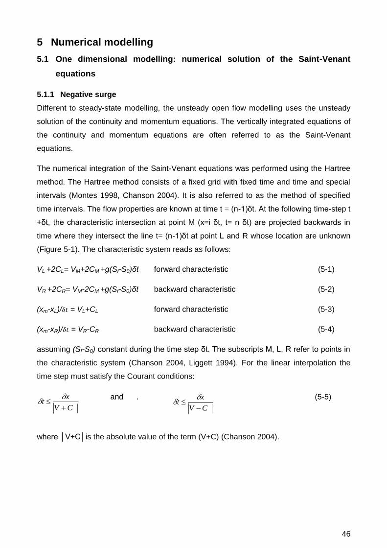
46

CV

xt

CV

xt

5 Numerical modelling

5.1 One dimensional modelling: numerical solution of the Saint-Venant

equations


Different to steady-state modelling, the unsteady open flow modelling uses the unsteady

solution of the continuity and momentum equations. The vertically integrated equations of

the continuity and momentum equations are often referred to as the Saint-Venant

equations.

The numerical integration of the Saint-Venant equations was performed using the Hartree

method. The Hartree method consists of a fixed grid with fixed time and time and special

intervals (Montes 1998, Chanson 2004). It is also referred to as the method of specified

time intervals. The flow properties are known at time t = (n-1)δt. At the following time-step t

+δt, the characteristic intersection at point M (x=i δt, t= n δt) are projected backwards in

time where they intersect the line t= (n-1)δt at point L and R whose location are unknown

(Figure 5-1). The characteristic system reads as follows:

VL +2CL= VM+2CM +g(Sf-S0)δt forward characteristic (5-1)

VR +2CR= VM-2CM +g(Sf-S0)δt backward characteristic (5-2)

(xm-xL)/ = VL+CL forward characteristic (5-3)

(xm-xR)/ = VR-CR backward characteristic (5-4)

assuming (Sf-S0) constant during the time step δt. The subscripts M, L, R refer to points in

the characteristic system (Chanson 2004, Liggett 1994). For the linear interpolation the

time step must satisfy the Courant conditions:

and

. (5-5)

where │V+C│is the absolute value of the term (V+C) (Chanson 2004).

47

Figure 5-1: Numerical integration of the methods of characteristics by the Hartree methods (Chanson

2004)

Both the analytical solution using the simple wave method and numerical model data were

compared with the physical data (Figure 5-2). The analytical solution based upon the

simple wave theory compared well with the physical data. The numerical solution of the

Saint-Venant equations using the Darcy friction factors f=0.015, f=0.025 and f=0.035 also

gave some good results. Most computer software packages use the numerical solution of

the Saint-Venant equations for solving one-dimensional flows. Figure 5-2 shows the best

agreement with the recorded ADM data was reached by the simple wave solution.

Therefore, one may argue that the analytical solution of the Saint-Venant equations did

match the physical results better than the numerical solutions or friction effects are

negligible.

Note however, that the present flume had a rectangular cross-section and was lined with

PVC and glass. Therefore, there was a small boundary friction. In natural channels, the

surface roughness is likely to be greater than in a laboratory setting and it might be

necessary to include different friction factors.

48

Figure 5-2: Dimensionless unsteady free-surface profile during the negative surge with 20 l/s

discharge and a 30 mm gate opening


The simple wave method was compared with the recorded acoustic displacement meter

data for the positive surge at x=6 m. Figure 5-3 illustrates that the analytical solution based

upon the simple wave theory did not compare well with the physical data. The simple wave

solution overestimates the celerity of the surge and underestimates the height of the surge

front. The simple wave method only allows calculating the timing of the surge front and the

water level increase. There was a difference of 7.8 s between the arrivals of the surge

front of the simple wave method compared to the physical data.

Figure 5-3: Dimensionless unsteady free-surface profile during the positive surge with 20 l/s

discharge and a 30 mm gate opening

t *(g/d0)^0.5

d/d 0

0 5 10 15 20 25 30 35 40 45 50 55

0.5

0.55

0.6

0.65

0.7

0.75

0.8

0.85

0.9

0.95

1

1.05

1.1

Data x=10.8 m

Data x=6 m

Simple Wave

SVE (f=0.0015)

SVE (f=0.025)

SVE (f=0.035)

Data x = 10.8 m

Data x = 6.0 m

Ideal gate closure (x=10.8m)

Simple wave (x=6 m)

SVE (f=0.015)

SVE (f=0.025)

SVE (f=0.035)

t*(g/d0)^0.5

d/d

0

0 10 20 30 40 50 60 70 80 90 100 110 120 130 1400.9

1

1.1

1.2

1.3

1.4

1.5

1.6

1.7

1.8

ADM Data x= 6 m

Simple wave

Data x=6 mSimple wave

49

5.2 Two dimensional modelling with Flow-3D

Flow-3DTM is a CFD model developed by Flow Science Inc.. Flow-3DTM calculates the

three velocity components (Vx, Vy, Vz) and pressures at the nodes of an orthogonal finite

difference grid, using a range of turbulence models. Flow-3DTM has the capabilities of

modelling free surface flows using the Volume of Fluid (VOF) method.

The models were set up using Flow-3DTM version 9.3. The viscosity and velocity

fluctuations option was selected with Newtonian viscosity and the renormalisation group

(RNG) turbulence model that used a dynamically computed maximum velocity fluctuations

mixing length.

The RNG model was selected because it was recommended as the most robust

turbulence model available within the Flow-3DTM modelling software (Flow-3D user manual

2007).

The geometry for the models was a simple rectangular channel with the same width and

depth as the experimental channel the length of the channel was extended by 0.8 m to

reduce boundary effects. The gate was simulated using the general moving object (GMO).

The GMO settings were set as prescribed motion with 6 degree of freedom (6-DOF).

The initial location of the reference point was selected in the middle of the gate at

x=11.2 m, y=0.25 m and z=0.25 m. The gate was operated using the translational velocity

component in the space system with a velocity of a non-sinusoidal movement in the z

direction of -1 m/s for the positive surge and +1 m/s for the negative surge. The gate

opening was selected to maximise model stability. The gate movement for the simulations

was vertical, which is different from the gate operation in the experimental setup, where

the gate opens in a semi-circular movement.

The selection of mesh size is essential for both the accuracy of the result and the

simulation times. Therefore, a sensitivity analysis was performed using three different

uniform mesh sizes of 5 mm, 15 mm and 30 mm. Smaller sizes have been tried out,

however, due to time limitations and model stability the smallest size chosen was 5 mm.

The results of the sensitivity analysis are further discussed in the following sections.

The selection of appropriate boundary conditions is essential for the accuracy of the

simulations. The boundary conditions are summarised in Table 5-1. However, there are

several other boundary options available in the software that could be applied for the

models in this study.

50

The choice of the boundary options was made to replicate the steady flow state prior to the

surge generation as closely to the experimental conditions as possible.

Table 5-1: Boundary conditions for Flow-3DTM

models

XMin XMax YMin YMax ZMin ZMax

Negative surge P P S S W S

Positive Surge Q P S S W S

Notes; P is the specified pressure boundary; S is the symmetry boundary; W is the wall boundary and Q stands for the

volume flow rate boundary.


A sensitivity analysis was performed to assess the impact of mesh size on the surface

profile of the negative surge. The results are presented in Figure 5-4. The Flow-3DTM

simulation replicated the experimental data for the negative surge reasonably well.

However, all the simulation using the 5 mm, 15 mm and 30 mm mesh sizes showed that

the water depth decreased more slowly than the recorded data. The uniform mesh size of

5 mm compared best with the measured results. The 15 mm and 30 mm mesh sizes

produced similar outcomes and no improvement was observed by using the 15 mm mesh

size compared to the 30 mm mesh size. The results recorded at x=6 m as presented in

Figure 5-4 (b) showed the same trend as observed at x=10.8 m using the 5 mm uniform

mesh size and compared the best to the measured data. The results calculated using the

Flow-3DTM software code, using a 5 mm mesh, are further illustrated in this section. The

velocity was assessed at four vertical elevations, which were closest to the measurements

taken in the experimental setup using the ADV and acoustic displacement meters. The

data were recorded on the centreline near the gate at x=10.5 m and further upstream at

x=6 m. The figures show dimensionless flow depth d/do as a function of dimensionless

time from gate closure 0/ dgt , where do is the initial water depth at x=6 m and

x=10.5 m respectively. Figure 5-5 presents some typical results in the form of

dimensionless time variation and water depth. For the negative surge, the surface water

profiles at the gate showed a steeper drop in water depth close to the gate (e.g. x=10.8 m)

compared to the observations further upstream at x=6 m, which is consistent with the

findings in previous sections (Figures 4-1 and 4-2). The longitudinal velocity Vx data were

closely linked with the depth profile. Due to the rapid drop in the depth profile only little

output was available near the gate for the vertical velocity recordings as further illustrated

in Appendix D.

51

Generally, the water depth decreased relatively gradually after the initial surge formation.

The free surface measurements showed some marked curvature near the surge leading

edge. The longitudinal velocity component increased at the same time as the water depth

decreased.

(a) x=10.8 m

(b) x=6 m

Figure 5-4: Dimensionless unsteady free-surface profile during the negative surge recorded and

simulated data

t *(g/d0)^0.5

d/d

0

0 5 10 15 20 25 30 35 40 45 50 55

0.5

0.55

0.6

0.65

0.7

0.75

0.8

0.85

0.9

0.95

1

1.05

1.1

Data x=10.8 m

Flow-3D 30 mm (x=10.8 m)

Flow-3D 15mm (x=10.8 m)

Flow-3D 5 mm (x=10.8 m)

ERROR BAR

Data (x = 10.8 m)

Flow-3D, mesh 30mm (x=10.8 m)



t *(g/d0)^0.5

d/d

0

20 22.5 25 27.5 30 32.5 35 37.5 40 42.5 45 47.5 50 52.5 55

0.5

0.55

0.6

0.65

0.7

0.75

0.8

0.85

0.9

0.95

1

1.05

1.1

Data x=6 m

Flow-3D 30 mm (x=6 m)



Data (x = 6.0 m)

Flow-3D,mesh 30mm (x=6 m)

Flow-3D, mesh 15mm (x=6 m)


52

(a) x=6 m, z=7.5 mm, Q=20 l/s, d0=0.20 m, initial gate opening 30 mm and 5 mm mesh size

(b) x=10.5 m, z=7.5 mm, Q=20 l/s, d0=0.064 m, initial gate opening 30 mm and 5 mm mesh size

Figure 5-5: Dimensionless velocity and depth measurements of a negative surge simulated using

Flow-3DTM


A sensitivity analysis was performed to assess the impact of mesh size on the surface

profile of the positive surge. The results are presented in Figure 5-6. The Flow-3DTM

simulations did not replicate the experimental data for the positive surge well. All the

simulation using the 5 mm, 15 mm and 30 mm uniform mesh sizes showed that the water

depth increased much less at the beginning and during the propagation of the surge. All

three simulations underestimated the water depth during the surge propagation. The

increase in mesh size was relatively sensitive to the timing of the surge front. The

simulation using a 15 mm uniform mesh provided good results compared to the recorded

data for the timing of the initial surge formation.

t*(g/d0)^0.5

Vx/V

0, V

y/V

0

d/d

0

1420 1425 1430 1435 1440 1445 1450 1455 1460 1465 1470 1475-0.5 0.52

0 0.6

0.5 0.68

1 0.76

1.5 0.84

2 0.92

2.5 1

3 1.08

3.5 1.16

Vx Vz d

t*(g/d0)^0.5

Vx/V

0,

Vy/V

0

d/d

0

1412 1414 1416 1418 1420 1422 1424 1426 1428 1430-0.5 0.2

0 0.3

0.5 0.4

1 0.5

1.5 0.6

2 0.7

2.5 0.8

3 0.9

3.5 1

4 1.1

4.5 1.2

5 1.3

Vx Vz d

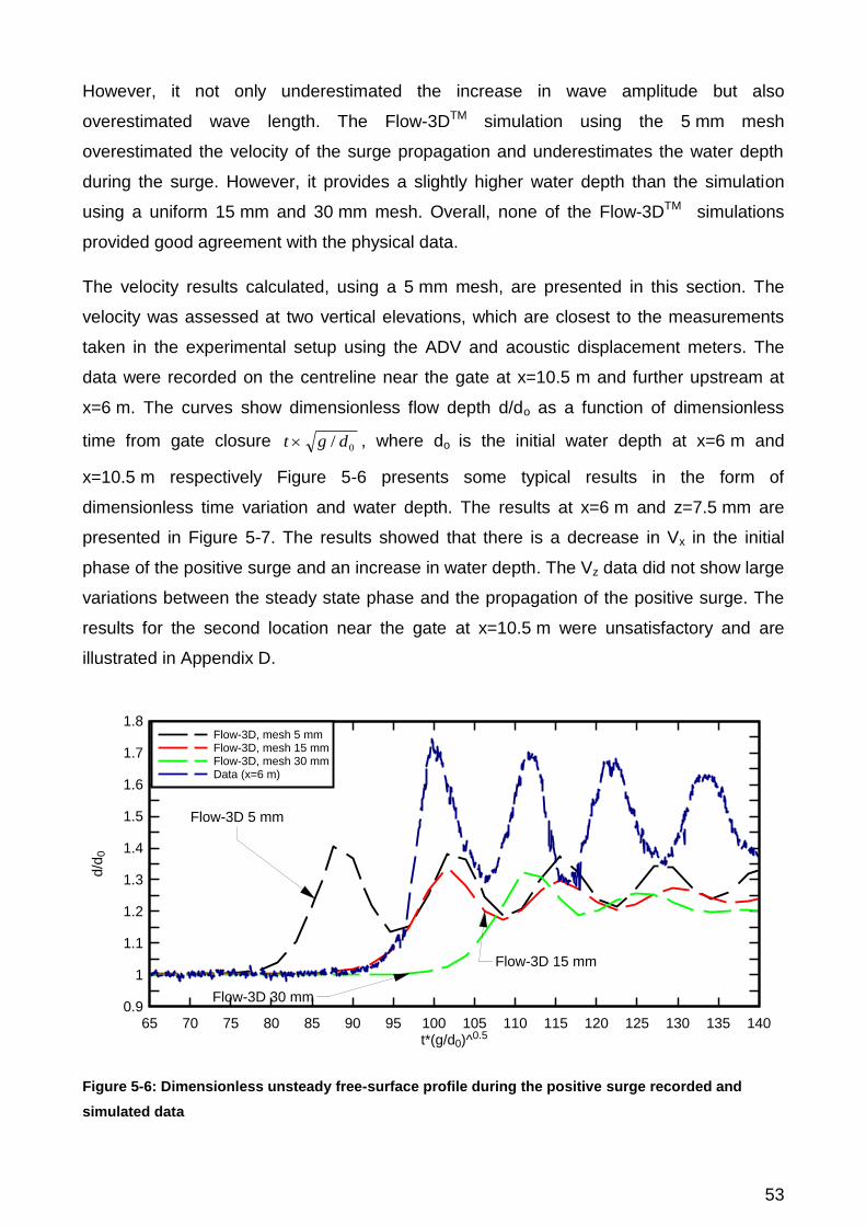
53

However, it not only underestimated the increase in wave amplitude but also

overestimated wave length. The Flow-3DTM simulation using the 5 mm mesh

overestimated the velocity of the surge propagation and underestimates the water depth

during the surge. However, it provides a slightly higher water depth than the simulation

using a uniform 15 mm and 30 mm mesh. Overall, none of the Flow-3DTM simulations

provided good agreement with the physical data.

The velocity results calculated, using a 5 mm mesh, are presented in this section. The

velocity was assessed at two vertical elevations, which are closest to the measurements

taken in the experimental setup using the ADV and acoustic displacement meters. The

data were recorded on the centreline near the gate at x=10.5 m and further upstream at

x=6 m. The curves show dimensionless flow depth d/do as a function of dimensionless

time from gate closure 0/ dgt , where do is the initial water depth at x=6 m and

x=10.5 m respectively Figure 5-6 presents some typical results in the form of

dimensionless time variation and water depth. The results at x=6 m and z=7.5 mm are

presented in Figure 5-7. The results showed that there is a decrease in Vx in the initial

phase of the positive surge and an increase in water depth. The Vz data did not show large

variations between the steady state phase and the propagation of the positive surge. The

results for the second location near the gate at x=10.5 m were unsatisfactory and are

illustrated in Appendix D.

Figure 5-6: Dimensionless unsteady free-surface profile during the positive surge recorded and

simulated data

t*(g/d0)^0.5

d/d

0

65 70 75 80 85 90 95 100 105 110 115 120 125 130 135 1400.9

1

1.1

1.2

1.3

1.4

1.5

1.6

1.7

1.8

Flow-3D 5 mm

Flow-3D 15 mm

Flow-3D 30 mm

Flow-3D, mesh 5 mmFlow-3D, mesh 15 mmFlow-3D, mesh 30 mmData (x=6 m)

54

Figure 5-7: Dimensionless velocity and depth measurements of a positive surge simulated using

Flow-3D at x=6 m, z=7.5 mm, Q=20 l/s, d0=0.064 m, initial gate opening 30 mm and 5 mm mesh size

t*(g/d0)^0.5

Vx/V

0,

Vy/V

0

d/d

0

2480 2488 2496 2504 2512 2520 2528 2536 2544 2552 2560-0.1 0.7

0 0.8

0.1 0.9

0.2 1

0.3 1.1

0.4 1.2

0.5 1.3

0.6 1.4

0.7 1.5

0.8 1.6

0.9 1.7

1 1.8

Vx Vz d

55

6 Comparison between numerical and physical data

6.1 Negative surge

6.1.1 Surface profile

The analytical solution and numerical model data were compared with experimental data

from ADM and video measurements (Figure 6-1). The video measurements at 10.8 m

compared well with the ADM data. However, near the gate the video data was slightly

higher than the ADM data. This might be related to the difficulty in estimating the water

surface near the gate form the video recordings. The simple wave method and the

numerical integration of the Saint-Venant equations compared well with the physical data.

The solutions with no or little friction compared better to the recorded data, than the ones

with higher friction factors. However, the laboratory flume had a rectangular cross-section

and was lined with PVC and glass. Therefore, it had a small boundary friction. In natural

channels, the surface roughness is likely to be greater than in a laboratory setting and it

might be necessary to include different friction factors. The Flow-3DTM results produced a

comparable output at x=10.8 m. It is suggested that the initial difference in the surface of

the water depth is related to the gate opening mechanism. As observed in previous

sections the instantaneous free surface measurements recorded a spike near the gate,

which might be due to the semi-circular movement of the gate, which pushed the water

upwards, before the natural progression of the surge. Initially the water depth was

simulated quite well using Flow-3DTM at x=10.8 m. However, it overestimated the water

depth shortly after the inflection points of the free surface and slightly underestimated it,

when the water depth reached the steady state flow. Overall, for the location near the gate

at x=10.8 m, the 5 mm mesh size matched best against experimental data compare to the

models with a uniform mesh size of 15 mm and 30 mm. The Flow-3DTM simulation at

x=6 m using 5 mm, 15 mm and 30 mm mesh sizes overestimated the water depth, but

produced a similar slope compared to the recoded data. The propagation of the negative

surge is replicated quite well for all the numerical method, with the surge front passing

through x=6 m, close to the measured data. The Flow-3DTM results showed a slight delay

in the surge front, which might be a result of the differences in gate opening mechanisms.

56

Figure 6-1: Dimensionless unsteady free-surface profile during the negative surge with Q=20 l/s and

a 30 mm gate opening

6.1.2 Turbulent velocities

The longitudinal velocities of the measured data were compared with the velocities of the

simple wave methods, the numerical integration of the Saint-Venant equations and the

outputs of the Flow-3DTM simulations. The results are presented in Figure 6-2. The

longitudinal velocities Vx were measured at z=6.69 mm, z=123.94 mm and z=135.2 mm.

The Flow-3DTM results for the model with 5 mm mesh size were output at locations closest

to the measured z values. The Vx velocity component for the simple wave method and

numerical integration of the Saint-Venant equations are the same for all vertical elevations.

All the velocities in the figures below are presented in dimensionless time and

dimensionless velocity components at x=6 m. The comparison of the simple wave method,

the numerical integration of the Saint-Venant equations and the Flow-3DTM simulation with

experimental data showed that there is an increase in the longitudinal velocity

components, as observed in all vertical locations.

t *(g/d0)^0.5

d/d

0

0 5 10 15 20 25 30 35 40 45 50 55

0.5

0.55

0.6

0.65

0.7

0.75

0.8

0.85

0.9

0.95

1

1.05

1.1

Data x=10.8 m

Data x=6 m

Simple Wave

SVE (f=0.0015)

SVE (f=0.025)

SVE (f=0.035)




Flow-3D 30 mm (x=10.8 m)

Flow-3D 15mm (x=10.8 m)

Flow-3D 5 mm (x=10.8 m)

Data (x = 10.8 m)

Data (x = 6.0 m)

Simple wave (x=6 m)

SVE (f=0.015)

SVE (f=0.025)

SVE (f=0.035)

Flow-3D,mesh 30mm (x=6 m)






Data (x=6m) Video

Data (x=10.8m) Video

57

However, the analytical method and the numerical integration generally overestimated the

longitudinal velocity component Vx for all vertical elevations.

The longitudinal velocity at z=135.2 mm showed the best agreement of the simple wave

methods and the numerical integration of the Saint-Venant equations with measured data.

The analytical method and numerical integration of the Saint-Venant equations

overestimated the longitudinal velocity component Vx close to the channel bed. Overall,

the analytical method compared best with the recorded Vx velocity component of the

negative surge. It replicated the longitudinal velocity trend at z=135.2 mm very closely.

The numerical integration of the Saint-Venant equations using different Darcy friction

factors compared reasonably well with the measured data. Generally, the results using the

highest friction factor f=0.035 overestimated the velocities the most, while the results of the

numerical integration of the Sain-Venant equations using the lowest Darcy friction factor

f=0.015 compared better with the measured data. This confirms the assumption made in

previous sections that for the experimental setup used in this the friction effect is negligible

for the negative surge.

The Flow-3DTM results generally underestimated the velocities for the negative surge for all

vertical elevations. The velocities before the surge passage were a close match to the

recorded data. The very initial stage of the surge propagation replicated the measured

data well. The Flow-3DTM simulation underestimated the velocities considerably during the

surge passage for all vertical elevations. The Flow-3DTM simulation compared best for

z=123.94 mm, compared to z=6.69 mm and z=135.2 mm. The much lower Vx values

during the surge propagation at z=6.69 mm suggested that the model did not represent the

physical processes closest to the channel bed. This was consistent with velocities of the

analytical and the numerical integration of the Saint-Venant equations, which showed the

biggest differences closest to the channel bed when compared with measured data. The

Flow-3DTM results presented are for the model setup as discussed in section 5.2. A

different model setup may lead to different findings.

In general, the simple wave methods produced good results when compared to the

experimental data. It was also the least time consuming method tested in this study. The

Flow-3DTM models were easy to setup, however, the choice of input parameters required

the user to have detailed knowledge of all the fluid properties. Also, Flow-3DTM simulations

were both time and computational intensive.

58

On the other hand, the simple wave method and the numerical integration of the Saint-

Venant equations required an initial input time series for the boundary setup and therefore,

would not be able to calculate the surge propagation without the availability of the input

data.

(a) z=6.69 mm, Q=20 l/s and 30 mm gate opening

(b) z=123.94 mm, Q=20 l/s and 30 mm gate opening

Figure 6-2: Comparison of the dimensionless longitudinal velocity components Vx derived from

analytical and numerical methods with measured data at x=6 m - Flow-3DTM

calculations performed

with 5 mm mesh size (cont’d).

t*(g/d0)^0.5

Vx/V

0

d/d

0

0 3 6 9 12 15 18 21 24 27 30 33 36 39 42 45 48 51 54 57 600 0.48

0.4 0.54

0.8 0.6

1.2 0.66

1.6 0.72

2 0.78

2.4 0.84

2.8 0.9

3.2 0.96

3.6 1.02

4 1.08

Water Depth

Vx- ADVVx- Flow-3DVx- SVE (f=0.015)

Vx- SVE (f=0.035)Vx- SVE (f=0.025)Vx- Simple Wave

t*(g/d0)^0.5

Vx/V

0

d/d

0

0 3 6 9 12 15 18 21 24 27 30 33 36 39 42 45 48 51 54 57 600 0.48

0.4 0.54

0.8 0.6

1.2 0.66

1.6 0.72

2 0.78

2.4 0.84

2.8 0.9

3.2 0.96

3.6 1.02

4 1.08

Water Depth



59

(c) z=135.2 mm, Q=20 l/s and 30 mm gate opening


analytical and numerical methods with measured data at x=6 m - Flow-3DTM

calculations performed

with 5 mm mesh size.

6.2 Positive surge

6.2.1 Surface profile

The simple wave method was used to obtain the analytical solution of the Saint-Venant

equations for the positive surge. The result was compared to surface water profile data

measured with acoustic displacement meters (Figure 6-3). The simple wave method did

not provide good results for the positive surge. There was a difference of 7.8 s between

the arrival of the surge front of the simple wave method and the physical data. In addition,

the wave amplitude was much lower than the amplitude observed in the recorded data.

The two-dimensional Flow-3DTM model was tested against physical data. The results are

presented in Figure 6-3. There was a substantial difference between the timing of the initial

surge formation between the three Flow-3DTM tests using 5 mm, 15 mm and 30 mm mesh

sizes. The Flow-3DTM model with a mesh 15 mm mesh size replicated the timing of the

initial surge formation the best, but it underestimated the wave amplitude. In the Flow-3DTM

model with a uniform mesh size of 5 mm, the initial formation of the positive surge

occurred much earlier than in the physical data. Although the wave amplitude was slightly

larger than in the other two Flow-3DTM configurations, it was still fundamentally

underestimated. The simple wave method and the Flow-3DTM simulation with a 5 mm

mesh provided simular results regarding the wave amplitude. Overall, all three Flow-3DTM

configurations and the simple wave methods did not compare well with the physical data.

t*(g/d0)^0.5

Vx/V

0

d/d

0

0 3 6 9 12 15 18 21 24 27 30 33 36 39 42 45 48 51 54 57 600 0.48

0.4 0.54

0.8 0.6

1.2 0.66

1.6 0.72

2 0.78

2.4 0.84

2.8 0.9

3.2 0.96

3.6 1.02

4 1.08

Water Depth



60

Figure 6-3: Unsteady free-surface profile during the positive surge

6.2.2 Turbulent velocities

The velocities of the Flow-3DTM model with a 5 mm uniform mesh size were compared to

experimental data. The Flow-3DTM model with a 5 mm mesh size was chosen because it

had a more detailed vertical velocity profile, compared to the 15 mm and 30 mm mesh size

models. The results are shown in dimensionless terms in Figure 6-4.

The results of the Flow-3D simulations showed a sharp deceleration of the longitudinal

velocity Vx, which was also observed in the physical data. Also, the results showed an

undular velocity pattern that is similar to the recorded data. The measured velocity data

were selected at z/d0=0.1 and z/d0=0.4. The Flow-3DTM results, recorded a larger velocity

at z/d0=0.4 than at z/d0=0.1. As expected, the velocities for the Flow-3DTM model were

smaller than the measured data. The sharp discontinuity in terms of the longitudinal

velocities occurred earlier in the Flow-3DTM model than in the measured data. This was

consistent with the earlier timing of the initial surge formation (section 6.2.1). While the

velocity at z=22.5 mm was close to the observed velocities, the velocity at z=7.5, was

smaller than the experimental data. This might be linked with the smaller wave amplitude

observed in the previous section.

Other studies, by Simon et al. (2011) and Lubin et al. (2010) found that the computation of

positive surges using a CFD code may be impacted by boundary conditions.

While the results of these studies provided good agreement of the surge flow patterns,

they also stated that the velocity profiles were not completely satisfying.

t*(g/d0)^0.5

d/d

0

0 10 20 30 40 50 60 70 80 90 100 110 120 130 1400.9

1

1.1

1.2

1.3

1.4

1.5

1.6

1.7

1.8

Flow-3D 5 mm

Flow-3D 15 mm

Flow-3D 30 mm

ADM Data x= 6 m

Simple wave

Flow-3D, mesh 5 mmFlow-3D, mesh 15 mmFlow-3D, mesh 30 mmData (x=6 m)Simple wave

61

The presented data showed that the surge generation immediately upstream of the gate

was an intense turbulent process, which cannot be modelled easily, with one-dimensional

equations, or a limited CFD model.

The difficulty to compute an accurate velocity profile for a positive surge, results in the

inaccuracy of the timing of the initial surge formation. It might be concluded that the

velocity profile and the turbulent mixing in positive surges are much more complex than in

negative surges. Also, the simulation of positive surges using CFD codes is still in its early

stages and the results should be validated against physical data.

(a) z/d0=0.1

(b) z/d0=0.4


analytical and numerical methods with measured data at x=6 m - Flow-3D calculations performed

with 5 mm mesh size.

t*(g/d0)^0.5

Vx/

V0

d/d

0

0 10 20 30 40 50 60 70 80 90 100 110 120 130 140-0.5 0.8

-0.3 0.9

-0.1 1

0.1 1.1

0.3 1.2

0.5 1.3

0.7 1.4

0.9 1.5

1.1 1.6

1.3 1.7

1.5 1.8

Water DepthData z=6.69 mmFlow-3D z=7.5mm

t*(g/d0)^0.5

Vx/

V0

d/d

0

0 10 20 30 40 50 60 70 80 90 100 110 120 130 140-0.5 0.8

-0.3 0.9

-0.1 1

0.1 1.1

0.3 1.2

0.5 1.3

0.7 1.4

0.9 1.5

1.1 1.6

1.3 1.7

1.5 1.8

Water DepthData z=25.01 mmFlow-3D z=22.5 mm

62

7 Conclusion

Unsteady open channel flow data were collected during the upstream propagation of

negative and positive surges. Both, physical and numerical modelling, were performed.

Some detailed measurements of free-surface fluctuations were recorded using non-

intrusive techniques, including acoustic displacement meters and video recordings.

Velocity measurements were sampled with high temporal and spatial resolution using an

ADV (200 Hz) at four vertical elevations and two longitudinal locations. The velocity and

water depth results were ensemble-averaged for both negative and positive surges. The

results showed that the water curvature of the negative surge was steeper near the gate at

x=10.5 m compared to further upstream at x=6 m. Both the instantaneous and ensemble-

average data showed that in the negative surge the inflection point of the water surface

and the longitudinal velocity Vx occurred simultaneously. Also, an increase in Vx was

observed at all elevations during the surge passage. For the positive surge the

propagation of the bore and the velocity fluctuations characteristics supported earlier

findings by Koch and Chanson (2009) and Docherty and Chanson (2010). The surge was

a major discontinuity in terms of the free-surface elevations, and a deceleration of the

longitudinal velocities Vx was observed during the surge passage.

The free-surface profile was analysed analytically using the simple wave solution of the

Saint-Venant equations. The analytical results in terms of water depth compared well with

the experimental results at x=6 m for the negative surge, but provided poorer results for

the positive surge. The numerical integration of the Saint-Venant equations compared

reasonably well with the physical data for the negative surge, in terms of both water depth

and longitudinal velocities. The longitudinal velocities where slightly overestimated

resulting in the underestimation of water depth. For the negative surge, the results of Flow-

3DTM simulations compared reasonably well with the measured data, but underestimated

the velocities resulting in an overestimation of the water surface. For the positive surge,

the analytical method and the computational analysis using Flow-3DTM did not compare

well with the physical data. All the models underestimated the water depth at both the

initial stage of the surge and during surge propagation. The simple wave solution and

Flow-3DTM simulation, with a uniform mesh size of 5 mm overestimated the velocities of

the positive surge. The timing of the positive surge formation was best simulated by the

Flow-3DTM model with 15 mm mesh size.

63

This study had two aims. First, to analyse the propagation and velocity fluctuations

characteristics of positive and negative surges, second, to validate the analytical and

numerical techniques against the physical data sets.

The study resulted in a number of significant outcomes:

1. High quality benchmark data was collected. Complete data sets including

simultaneous data for depth and velocity were collected specifically with high spatial

and temporal resolution in unsteady open channel flows. The physical data provide

a unique data set for future numerical model validation.

2. The study showed that theoretical models may be applied successfully to unsteady

flow situations, with simple channel geometry. The theoretical models are often

overlooked for more complex numerical methods to solve unsteady open channel

flow situations. However, a theoretical model may provide better results in some

unsteady flow situations in simple channel geometries as shown for the negative

surge herein.

3. The one-dimensional (1D) modelling compared well with physical data and better

than a more complex CFD model for the negative surge. Although one-dimensional

modelling is popular in the engineering industry, some engineers believe that CFD

modelling is more capable. This study showed that the numerical integration of the

Saint-Venant equations compared well with the measured data for the negative

surge, while CFD modelling did not match physical data in highly unsteady open

channel flows within the setup used in this study.

4. The study showed that the selection of the appropriate mesh size for CFD

simulations is critical and that a sensitivity analysis is essential for highly unsteady

open channel flows, together with access to a solid validation data set. In the

absence of quality validation data, the user would not be able to determine the

appropriate mesh size, which might results in substantial differences of model

outcomes.

5. The present experience demonstrated that the usage of a commercial CFD

package requires some solid understanding of all the properties of the software,

including the basic equations, the velocity fluctuations model(s) and the definition of

the boundary conditions.

64

6. A negative surge is associated with a relative gentle decrease in water elevation.

Although, the pressure distributions might not be hydrostatic at the leading edge of

the surge, the Saint-Venant equations provide reasonably accurate predictions of

the surge properties using both analytical and numerical approaches.

7. In a positive surge, the surge front is a sharp discontinuity in terms of water

elevations, velocities and pressure. The present data showed that the surge

generation immediately upstream of the gate is an intense turbulent process, which

cannot be simply modelled neither, with one-dimensional equations nor a limited

CFD model.

8. Highly unsteady open channel flows remain a challenge for professional engineers

and researchers.

65

References

ARIC’O, C., NASELLO, C., and TUCCIARELLI, T. (2007). “A Marching in Space and Time

(MAST) Solver of the Shallow Water Equations, Part II: The2-D model.” Adv. Water Res.,

Vol. 30, No.5, pp. 1253–1271.

ALCRUDO, F. and SORARES FRAZAO, S. (1998). “Conclusions from 1st CADAM

Meeting.” Proc. of 1st CADAM Meeting, Paper 5, Wallingford.

ALTINAKAR, M.S., MATHEU, E.E, and MCGRANTH, M.Z. (2009a). “New Generation

Modeling and Decision Support Tools for Studying Impacts of Dam Failures. Dam Safety

2009.” Proc., ASDSO 2009 Annual Conference, Sept. 27-October 1, Hollywood, FL (CD-

Rom). Association of State Dam Safety Officials, Lexington, KY.

BARRÉ de SAINT-VENANT, A.J.C. (1871a). "Théorie et Equations Générales du

Mouvement Non Permanent des Eaux Courantes." Comptes Rendus des séances de

l'Académie des Sciences, Paris, France, Séance 17 July 1871, Vol. 73, pp. 147-154.

BARRÉ de SAINT-VENANT, A.J.C. (1871b). "Théorie du Mouvement Non Permanent des

Eaux, avec Application aux Crues de Rivières et à l'Introduction des Marées dans leur Lit."

Comptes Rendus des séances de l'Académie des Sciences, Paris, France, Vol. 73, No. 4,

pp. 237-240.

BAZIN, H. (1865a). "Recherches Expérimentales sur l'Ecoulement de l'Eau dans les

Canaux Découverts." ('Experimental Research on Water Flow in Open Channels.')

Mémoires presents par divers savants à l'Académie des Sciences, Paris, France, Vol. 19,

pp. 1-494.

BAZIN, H. (1865b). "Recherches Expérimentales sur la Propagation des Ondes."

('Experimental Research on Wave Propagation.') Mémoires présentés par divers savants

à l'Académie des Sciences, Paris, France, Vol. 19, pp. 495-644.

BENET, F., and CUNGE, J.A. (1971). "Analysis of Experiments on Secondary Undulations

caused by Surge Waves in Trapezoidal Channels." Jl of Hyd. Res., IAHR, Vol. 9, No. 1,

pp. 11-33.

BENJAMIN, T.B., and LIGHTHILL, M.J. (1954). "On Cnoidal Waves and Bores." Proc.

Royal Soc. Of London, Series A, Math. & Phys. Sc., Vol. 224, No. 1159, pp. 448-460.

66

BISCARINI, C., DI FRANCESCO, S. and MANCIOLA P. (2009). “CFD Modelling Approach

for Dam Break Flow Studies.” Hydrol. Earth Syst. Sci., Vol. 14, pp.705–718.

BOUSSINESQ, J.V. (1877). "Essai sur la Théorie des Eaux Courantes." ('Essay on the

Theory of Water Flow.') Mémoires présentés par divers savants à l'Académie des

Sciences, Paris, France, Vol. 23, Série 3, No. 1, supplément 24, pp. 1-680.

CAVAILLE, Y. (1965). "Contribution à l'Etude de l'Ecoulement Variable Accompagnant la

Vidange Brusque d'une Retenue." ('Contribution to the Study of Unsteady Flow Following

a Dam Break.') Publ. Scient. et Techn. du Ministère de l'Air, No. 410, Paris, France, 165

pages.

CHANSON, H. (1995). "Flow Characteristics of Undular Hydraulic Jumps. Comparison

with Near-Critical Flows." Report CH45/95, Dept. Of Civil Engineering, University of

Queensland, Australia, June, 202 pages.

CHANSON, H., AOKI, S., and MARUYAMA, M. (2000). "Experimental Investigations of

Wave Runup Downstream of Nappe Impact. Applications to Flood Wave Resulting from

Dam Overtopping and Tsunami Wave Runup." Coastal/Ocean Engineering Report, No.

COE00-2, Dept. of Architecture and Civil Eng., Toyohashi University of Technology,

Japan, 38 pages.

CHANSON, H. (2004). "The Hydraulics of Open Channel Flows: An Introduction."

Butterworth-Heinemann, Oxford, UK, 2nd edition, 630 pages.

{http://www.uq.edu.au/~e2hchans/reprints/book3_2.htm}

CHANSON, H. (2005). "Le Tsunami du 26 Décembre 2004: un Phénomène Hydraulique

d'Ampleur Internationale. Premier Constats." ('The 26 December 2004 Tsunami: a

Hydraulic Engineering Phenomenon of International Significance. First Comments') Jl La

Houille Blanche, No. 2, pp. 25-32.

CHANSON, H. (2010). "Unsteady Turbulence in Tidal Bores: the Effects of Bed

Roughness." Journal of Waterway, Port, Coastal, and Ocean Engineering, ASCE, Vol. 136

(ISSN 0733-950X).

CHANSON, H. (2011). "Turbulent Shear Stresses in Hydraulic Jumps, Bores and

Decelerating Surges.” Earth Surf. Processes, Vol. 36, pp.180-189.

67

CUNGE, J.A., F.M. HOLLY and Jr. and A. VERWEY (1980). “Practical Aspects of

Computational River Hydraulics. London, Pitman.

CUNGE, J.A. (2003). Undular bores and secondary waves -experiments and hybrid finite-

volume modelling.”J. Hyd. Res., IAHR, Vol 41, No.5,pp. 557–558.

DE MAIO, A., SAVI, F., and SCLAFANI, L (2004). “Three-dimensional Mathematical

Simulation of Dambreak Flow.” Proceeding of IASTED conferences – Environmental

Modelling and Simulation ISBN: 0-88986-441-1 St. Thomas, US Virgin Island.

DE MARCHI, G. (1945). “Ondi di depressione provocato da apperatura di paratoia in un

canale in definito.” L’Energia Elettrica , Vol. 22(1/2), pp. 1-13.

DOCHERTY, N.J., and CHANSON, H. (2010). "Characterisation of Unsteady Turbulence

in Breaking Tidal Bores including the Effects of Bed Roughness." Hydraulic Model Report

No. CH76/10, School of Civil Engineering, The University of Queensland, Brisbane,

Australia, 112 pages.

DRESSLER, R.F. (1952). "Hydraulic Resistance Effect upon the Dam-Break Functions." Jl

of Research, Natl. Bureau of Standards, Vol. 49, No. 3, pp. 217-225.

DRESSLER, R. (1954). "Comparison of Theories and Experiments for the Hydraulic Dam-

Break Wave." Proc. Intl Assoc. of Scientific Hydrology Assemblée Générale, Rome, Italy,

Vol. 3, No.38, pp. 319-328.

ESTRADE, J. (1967). "Contribution à l'Etude de la Suppression d'un Barrage. Phase

Initiale de l'Ecoulement." ('Contribution to the Study of Dam Break. Initial Stages of the

Wave.') Bulletin de la Direction des Etudes et Recherches, Series A, Nucléaire,

Hydraulique et Thermique, EDF Chatou, France, No. 1, pp. 3-128.

ESTRADE, J., and MARTINOT-LAGARDE, A. (1964). "Ecoulement Consécutif à la

Suppression d'un Barrage dans un Canal Horizontal de Section Rectangulaire." ('Dam

Break Wave Flow in a Horizontal Rectangular Canal.') Comptes-Rendus de l'Académie

des Sciences de Paris, Vol. 259, 21 December, Group 2, pp. 4502-4505.

FAVRE, H. (1935). "Etude Théorique et Expérimentale des Ondes de Translation dans les

Canaux Découverts." ('Theoretical and Experimental Study of Travelling Surges in Open

Channels.') Dunod, Paris, France.

68

FAURE, J., and NAHAS, N. (1961). "Etude Numérique et Expérimentale d'Intumescences

à Forte Courbure du Front." ('A Numerical and Experimental Study of Steep-Fronted

Solitary Waves.')Jl La Houille Blanche, No. 5, pp. 576-586. Discussion: No. 5, p. 587.

FLOW SCIENCE, INC. (2007). “Flow-3D User’s Manuals”, Version 9.2, Santa Fe, NM

FRACCAROLLO, L. and TORO, E. F.(1995). “Experimental and Numerical Assessment of

the Shallow Water Model for Two-Dimensional Dam-Break Problems, Jl. Hydr. Res., Vol.

33, pp. 843–864.

FURUYAMA, S.I. and CHANSON, H. (2010). “A numerical simulation of a tidal bore flow.”

Costal Engineering Journal, Vol. 52, No. 3, pp.215-234.

G’OMEZ-GESTEIRA, M. and DALRYMPLE, R. A. (2004). “Using a Three Dimensional

Smoothed Particle Hydrodynamics Method for Wave Impact on a Tall Structure. “J.

Waterway, Port, Coastal and Ocean Eng., Vol. 130, No. 2, pp. 63–69.

GORING, D.G., and NIKORA, V.I. (2002). “Despiking Acoustic Doppler Velocimeter Data.”

Jl of Hyd. Engrg., ASCE, Vol. 128, No. 1, pp. 117-126. Discussion: Vol. 129, No. 6,

pp.484-489.

HENDERSON, F.M. (1966). "Open Channel Flow." MacMillan Company, New York, USA.

HORMADKA, T. V., BERENBROCK, C. E., FRECKLETON, J. R., and GUYMON, G. L

(1985). “A Two-Dimensional Dam-Break Flood Plain Model, Adv. Wat. Res., Vol. 8, 7–14

March.

HORNUNG, H.G., WILLERT, C., and TURNER, S. (1995). "The Flow Field Downstream of

a Hydraulic Jump." Jl of Fluid Mech., Vol. 287, pp. 299-316.

JIN, M and D. L. FREAD (1997). “Dynamic flood routing with explicit and implicit numerical

solution schemes.” Jl of Hyd. Engrg, ASCE, Vol. 123, No.3,pp. 166-173.

KOCH, C., and CHANSON, H. (2005). "An Experimental Study of Tidal Bores and Positive

Surges: Hydrodynamics and Turbulence of the Bore Front." Report No. CH56/05, Dept. of

Civil Engineering, The University of Queensland, Brisbane, Australia, July, 170 pages.

KOCH, C., and CHANSON, H. (2009). "Turbulence Measurements in Positive Surges and

Bores." Jl of Hyd. Res., IAHR, Vol. 47, No. 1, pp. 29-40.

69

LAUBER, G. (1997). "Experimente zur Talsperrenbruchwelle im glatten geneigten

Rechteckkanal." ('Dam Break Wave Experiments in Rectangular Channels.') Ph.D. thesis,

VAW-ETH, Zürich,Switzerland. (also Mitteilungen der Versuchsanstalt fur Wasserbau,

Hydrologie und Glaziologie, ETH-Zurich, Switzerland, No. 152).

LAUBER, G., and HAGER, W.H. (1998). “Experiment to Dambreak Wave: Horizontal

Channel.” Jl of Hyd. Res., IAHR, Vol. 36, No. 3, pp. 291-307.

LEMMIN, U., and LHERMITTE, R. (1999). “ ADV Measurements of Turbulence: can we

Improve their Interpretation? Discussion.” Jl of Hyd. Engrg., ASCE, Vol. 125, No. 6, pp.

987-988.

LEMOINE, R. (1948). "Sur les Ondes Positives de Translation dans les Canaux et sur le

Ressaut Ondulé de Faible Amplitude." ('On the Positive Surges in Channels and on the

Undular Jumps of Low Wave Height.') Jl La Houille Blanche, Mar-Apr., pp. 183-185.

LEWIS, A.W. (1972). "Field Studies of a Tidal Bore in the River Dee." M.Sc. thesis, Marine

Science Laboratories, University College of North Wales, Bangor, UK.

LEVIN, L. (1952). "Mouvement Non Permanent sur les Cours d'Eau à la Suite de Rupture

de Barrage." ('Unsteady Flow Motion Induced by a Dam Break.') Revue Générale de

l'Hydraulique, Vol. 18, pp. 297-315.

LIANG, D., LIN, B., and FALCONER, R. A. (2007). “Simulation of Rapidly Varying Flow

Using an Efficient TVD-MacCormack Scheme.” Int. J. Numer. Meth. Fl., Vol. 53, pp.811–

826.

LIGGETT, J.A. (1994). "Fluid Mechanics." McGraw-Hill, New York, USA.

LUBIN, P., GLOCKNER, S. and CHANSON, H. (2010). “Numerical simulation of a weak

breaking tidal bore.” Mech. Res. Comm., Vol.37, pp.119-121.

MADSEN, A., SVENDSEN, I.A and PAN, C.H. (2005). “Numerical simulation of tidal bores

and hydraulic jumps. “ Costal Eng., Vol. 52, pp. 409-433.

MANCIOLA, P., MAZZONI, A., and SAVI, F. (1994). ”Formation and Propagation of Steep

Waves: An Investigative Experimental Interpretation.” Proceedings of the Specialty

Conference Co-sponsored by ASCE-CNR/CNDCI-ENEL Spa, Milan, Italy, 29 June–1 July.

MARTIN, H. (1983). “Dam-break Wave in Horizontal Channels with Parallel and Divergent

Side Walls.” 20 IAHR Congress Moscow 2, pp.494-505.

70

MENENDEZ, A.N., and NAVARRO, F. (1990). “An Experimental Study of the Continuous

Breaking of a Dam.” Jl of Hyd. Res., IAHR, Vol.28, No.6, pp.753-772.

McLELLAND, S.J., and NICHOLAS, A.P. (2000).”A New Method for Evaluating Errors in

High-Frequency ADV Measurements.” Hydrological Processes, Vol.14, pp.351-366.

MOHAMMANDI, M.(2008). “Boundary Shear Stress Around Bridge Piers.” Am. J. Appl.

Sci., Vol. 5, No.11, pp. 1547–1551.

MONTES, J.S. (1998). "Hydraulics of Open Channel Flow." ASCE Press, New-York, USA,

697pages.

NAGATA, N., HOSODA, T., NAKATO, T., and MURAMOTO, Y. (2005). “Three-

Dimensional Numerical Model for Flow and Bed Deformation around River Hydraulic.” Jl.

Hyd. Engrg.-ASCE, Vol. 131, No.12, pp. 1074– 1087.

PEREGRINE, D.H. (1966). "Calculations of the Development of an Undular Bore." Jl. Fluid

Mech., Vol 25, pp.321-330.

QUECEDO, M., PASTOR, M., HERREROS, M.I., FERNANDEZ MERODO, J. A., and

ZHANG, Q. (2005). Comparison of Two Mathematical Models for Solving the Dam Break

Problem Using the FEM Method.” Comput. Method Appl. M., Vol. 194, No. 36–38, pp.

3984–4005.

RAJAR, R. (1973). “ Modèle Mathematique et Abaques sans Dimensions pour la

Determination de L’écoulement qui suit la Rupture d’un Barrage.” ICOLD Congress,

Madrid Q40(R34), pp. 503-521.

SANDER, J and HUTTER, K (1991). “On the development of the theory of the solitary

wave. A historical essay,” Acta Mech., Vol. 86, pp. 111–152.

SCHOKLITSCH, A. (1917). “Über Dambruchwellen." Sitzungberichten der Königliche

Akademie der Wissenschaften, Vienna, Vol. 126, Part IIa, pp. 1489-1514.

SERRE, F. (1953). "Contribution à l'Etude des Ecoulements Permanents et Variables dans

les Canaux." ('Contribution to the Study of Permanent and Non-Permanent Flows in

Channels.') Jl La Houille Blanche, Dec., pp. 830-872.

71

SIMON, B., LUBIN, P., GLOCKNER, S., and CHANSON, H. (2011). "Three-Dimensional

Numerical Simulation of the Hydrodynamics generated by a Weak Breaking Tidal Bore."

Proc. 34th IAHR World Congress, Brisbane, Australia, 26 June-1 July, Engineers Australia

Publication, Eric VALENTINE, Colin APELT, James BALL, Hubert CHANSON, Ron COX,

Rob ETTEMA, George KUCZERA, Martin LAMBERT, Bruce MELVILLE and Jane

SARGISON Editors, pp. 1133-1140.

SOAREZ FRAZAO, S. and ZECH, Y (2002). “Dam Break in Channels with 90 °bend.” Jl of

Hyd. Engrg -ASCE, Vol.128, No.11, pp. 956–968.

SOBEY, R.J. and DINGEMANS, M.W. (1992). “Rapidly varied flow analysis of undular

bore.“J. Waterway, Port, Coastal and Ocean Engrg., ASCE, Vol. 118, No.4, 417–436.

STRELKOFF, T. S and H. T. FALVEY (1993). “Numerical method used to model unsteady

canal flow.” Jl. of Hyd. Engrg., ASCE, Vol. 119, No. 4, pp. 637-655.

TAN, L. and CHU, V.H. (2010). “Lauber and Hager’s Dam-break Wave Data for Numerical

Model Validation.” Jl of Hyd. Res., Vol. 47, No.4, pp.524-528.

TELES DA SILVA, A.F. and PERERINE, D.H. (1990). “Nonsteady computations of undular

and breaking bores.” Proceeding of the 22nd International Congress Coastal Engineering,

Delft, The Netherlands, ASCE Publ., Vol. 1, pp. 1019–1032.

TOOMBES, L. and CHANSON, H. (2011). "Numerical Limitations of Hydraulic Models."

Proc. 34th IAHR World Congress, Brisbane, Australia, 26 June-1 July, Engineers Australia

Publication, Eric VALENTINE, Colin APELT, James BALL, Hubert CHANSON, Ron COX,

Rob ETTEMA, George KUCZERA, Martin LAMBERT, Bruce MELVILLE and Jane

SARGISON Editors, pp. 2322-2328.

TRESKE, A. (1994). "Undular Bores (Favre-Waves) in Open Channels - Experimental

Studies." Jl of Hyd. Res., IAHR, Vol. 32, No. 3, pp. 355-370. Discussion: Vol. 33, No. 3, pp.

274-278.

TRICKER, R.A.R. (1965).” Bores, Breakers, Waves and Wakes.” American Elsevier Publ.

Co., NewYork, USA.

TRIFFONOV, E.K. (1935). “Etudes Expérimentales de la Propagation d’une Onde Positive

le Long d’un fond sec. ”Bulletin des Congrès de Navigation, Bruxelles 10(19), pp. 66-77.

72

US CORPS OF ENGINEERS (1960). “Floods Resulting from Suddenly Breached Dams.

Miscellaneous Paper 2 (374), Report 1. UA Army Engineers Waterways Experiment

Station, Corps of engineers: Vicksburg, Mississippi.

VOULGARIS, G. and TOWNBRIDGE J.H. (1998). “Evaluation of the Acoustic Doppler

Velocimeter (ADV) for Turbulence Measurements.” J. Atmos. Oceanic. Technol, Vol 15,pp.

272-289.

WHAL, T.L. (2003). “Despiking Acoustic Doppler Velocimeter Data. Discussion.” Jl of Hyd.

Engrg., ASCE, Vol. 129, No. 6, pp. 484-487.

WILKINSON, D.L. and BANNER, M.L. (1977). “Undular bores.” Proceeding of 6th

Australasian Hydraulic and Fluid Mechanics Conference, Adelaide, Australia, 369–373.

XANTHOPOULOS, T. and KOUTITAS, C (1976). “Numerical Simulation of a Two

Dimensional Flood Wave Propagation Due to Dam-Failure, J. Hyd. Res., Vol. 14, No. 4,

pp. 321–331.

YEH, H.H. and MOK, K.M. (1990). “On turbulence in bores.” Physics of Fluids, Series A,

Vol.2, No.5, 821–828.

ZHANG W. and W. SUMMER (1994). “Computation of rapidly varied unsteady flows in

open channels and comparison with physical model and field experiments.”

Hydroinformatics ’94, A. Verwey, A. M. Minns, V. Babovic & C. Maksimovic (eds),

Balkema, Rotterdam 731-737.

ZIENKIEWICZ, O.C. and SANDOVER, J.A. (1957). “The undular surge wave.” Proceeding

of the 7th IAHR Congress,, Lisbon, Portugal, Vol. II, paper D25, D1–11.

A1

Appendix A – Photographs of the experiments

A-1Presentation

New experiments were performed in the hydraulic laboratory at the University of

Queensland. The channel was horizontal, 12 m long and 0.5 m wide. The sidewalls were

made of 0.45 m high glass panels and the bed was made of 12 mm thick PVC sheets.

Notation


L channel length (m);

Q volume flow rate (m3/s);

Vo initial velocity (m/s);

W channel width (m);


A3

Figure A-1: Propagation of a positive surge – Q=30 l/s, d0=6.4 cm, 25 frames per second,

initial gate opening of 40 mm and 11.2< x <10.48 m

A5

Figure A-2: Propagation of a negative surge – Q=20 l/s, d0=26 cm, 25 frames per second,

initial gate opening of 40 mm and 11.2< x <10.48 m

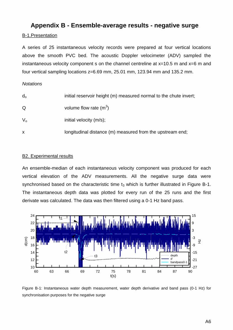
A6

Appendix B - Ensemble-average results - negative surge

B-1.Presentation

A series of 25 instantaneous velocity records were prepared at four vertical locations

above the smooth PVC bed. The acoustic Doppler velocimeter (ADV) sampled the

instantaneous velocity component s on the channel centreline at x=10.5 m and x=6 m and

four vertical sampling locations z=6.69 mm, 25.01 mm, 123.94 mm and 135.2 mm.

Notations


Q volume flow rate (m3)



B2. Experimental results


vertical elevation of the ADV measurements. All the negative surge data were

synchronised based on the characteristic time t3 which is further illustrated in Figure B-1.

The instantaneous depth data was plotted for every run of the 25 runs and the first

derivate was calculated. The data was then filtered using a 0-1 Hz band pass.

Figure B-1: Instantaneous water depth measurement, water depth derivative and band pass (0-1 Hz) for

synchronisation purposes for the negative surge

t(s)

d(c

m)

Hz

60 63 66 69 72 75 78 81 84 87 9010 -27

12 -21

14 -15

16 -9

18 -3

20 3

22 9

24 15

t3

t1

t2depthd'bandpass0-1

A7

The experimental results are shown in terms of ensemble-averaged median velocity

component as a function of time. Each graph includes the ensemble-averaged median

velocity component (Vx, Vy, Vz) the range of maximum to minimum velocities, the

differences between the 3rd and 4th quartiles (V75-V25) and 90% and 10% percentiles, (V90-

V10) and the ensemble-averaged water depth, dMedian.

(a) z=123.94 mm, x=6 m (con’t)

Figure B-3: Dimensionless ensemble-average median velocity VyMedian, difference between 3rd and 4th

quartiles (V75- V25) and 90% and 10% percentiles (V90- V10), and range of maximum to minimum velocities

(Vmax- Vmin) at x=6 m- From Top to bottom Vx, Vy, Vz (con’t)

t*(g/d0)0.5

dM

ed

ian/d

0

VxM

ed

ian/V

0,

Vxm

ax-V

xm

in/V

0,

Vx7

5-V

x2

5/V

0,

Vx9

0-V

x1

0/V

0,

85 87.5 90 92.5 95 97.5 100 102.5 105 107.5 110 112.5 115 117.5 1200.55 -1.6

0.6 -0.8

0.65 0

0.7 0.8

0.75 1.6

0.8 2.4

0.85 3.2

0.9 4

0.95 4.8

1 5.6

1.05 6.4

1.1 7.2

dMedian

VxMedian

Vxmax-Vxmin

Vx90-Vx10

Vx75-Vx25

t*(g/d0)0.5

dM

ed

ian/d

0

VyM

ed

ian/V

0,

Vym

ax-V

ym

in/V

0,

Vy7

5-V

y2

5/V

0,

Vy9

0-V

y1

0/V

0,

85 87.5 90 92.5 95 97.5 100 102.5 105 107.5 110 112.5 115 117.5 1200.55 -1.6

0.6 -0.8

0.65 0

0.7 0.8

0.75 1.6

0.8 2.4

0.85 3.2

0.9 4

0.95 4.8

1 5.6

1.05 6.4

1.1 7.2

dMedian

VyMedian

Vymax-Vymin

Vy90-Vy10

Vy75-Vy25

A8

(a) z=123.94 mm, x=6 m

(b) z= 135.2 mm, x=6 m (con’t)



(Vmax- Vmin) at x=6 m- From Top to bottom Vx, Vy, Vz (con’t)

t*(g/d0)0.5

dM

ed

ian/d

0

VzM

ed

ian/V

0,

Vzm

ax-V

zm

in/V

0,

Vz7

5-V

z2

5/V

0,

Vz9

0-V

z1

0/V

0,

85 87.5 90 92.5 95 97.5 100 102.5 105 107.5 110 112.5 115 117.5 1200.55 -1.6

0.6 -0.8

0.65 0

0.7 0.8

0.75 1.6

0.8 2.4

0.85 3.2

0.9 4

0.95 4.8

1 5.6

1.05 6.4

1.1 7.2

dMedian

VzMedian

Vzmax-Vzmin

Vz90-Vz10

Vz75-Vz25

t*(g/d0)0.5

dM

ed

ian/d

0

VxM

ed

ian/V

0,

Vxm

ax-V

xm

in/V

0,

Vx7

5-V

x2

5/V

0,

Vx9

0-V

x1

0/V

0,

85 87.5 90 92.5 95 97.5 100 102.5 105 107.5 110 112.5 115 117.5 1200.55 -1.6

0.6 -0.8

0.65 0

0.7 0.8

0.75 1.6

0.8 2.4

0.85 3.2

0.9 4

0.95 4.8

1 5.6

1.05 6.4

1.1 7.2

dMedian

VxMedian

Vxmax-Vxmin

Vx90-Vx10

Vx75-Vx25

A9

(b) z= 135.2 mm, x=6 m



(Vmax- Vmin) at x=6 m- From Top to bottom Vx, Vy, Vz

t*(g/d0)0.5

dM

ed

ian/d

0

VyM

ed

ian/V

0,

Vym

ax-V

ym

in/V

0,

Vy7

5-V

y2

5/V

0,

Vy9

0-V

y1

0/V

0,

85 87.5 90 92.5 95 97.5 100 102.5 105 107.5 110 112.5 115 117.5 1200.55 -1.6

0.6 -0.8

0.65 0

0.7 0.8

0.75 1.6

0.8 2.4

0.85 3.2

0.9 4

0.95 4.8

1 5.6

1.05 6.4

1.1 7.2

dMedian

VyMedian

Vymax-Vymin

Vy90-Vy10

Vy75-Vy25

t*(g/d0)0.5

dM

ed

ian/d

0

VzM

ed

ian/V

0,

Vzm

ax-V

zm

in/V

0,

Vz7

5-V

z2

5/V

0,

Vz9

0-V

z1

0/V

0,

85 87.5 90 92.5 95 97.5 100 102.5 105 107.5 110 112.5 115 117.5 1200.55 -1.6

0.6 -0.8

0.65 0

0.7 0.8

0.75 1.6

0.8 2.4

0.85 3.2

0.9 4

0.95 4.8

1 5.6

1.05 6.4

1.1 7.2

dMedian

VzMedian

Vzmax-Vzmin

Vz90-Vz10

Vz75-Vz25

A10

(a) z=25.01 mm, x=10.5 m (con’t)



(Vmax- Vmin) at x=10.5 m- From Top to bottom Vx, Vy, Vz (con’t)

t*(g/d0)0.5

dM

edia

n/d

0

VxM

edia

n/V

0,

Vxm

ax-V

xm

in/V

0,

Vx75-V

x25/V

0,

Vx90-V

x10/V

0,

65 66 67 68 69 70 71 72 73 74 750.55 -1.6

0.6 -0.8

0.65 0

0.7 0.8

0.75 1.6

0.8 2.4

0.85 3.2

0.9 4

0.95 4.8

1 5.6

1.05 6.4

1.1 7.2

dMedian

VxMedian

Vxmax-Vxmin

Vx90-Vx10

Vx75-Vx25

t*(g/d0)0.5

dM

edia

n/d

0

VyM

edia

n/V

0,

Vym

ax-V

ym

in/V

0,

Vy75-V

y25/V

0,

Vy90-V

y10/V

0,

65 66 67 68 69 70 71 72 73 74 750.55 -1.6

0.6 -0.8

0.65 0

0.7 0.8

0.75 1.6

0.8 2.4

0.85 3.2

0.9 4

0.95 4.8

1 5.6

1.05 6.4

1.1 7.2

dMedian

VyMedian

Vymax-Vymin

Vy90-Vy10

Vy75-Vy25

A11

(a) z=25.01 mm, x=10.5 m

(b) z=123.94 mm, x=10.5 m (con’t)




t*(g/d0)0.5

dM

edia

n/d

0

VzM

edia

n/V

0,

Vzm

ax-V

zm

in/V

0,

Vz75-V

z25/V

0,

Vz90-V

z10/V

0,

65 66 67 68 69 70 71 72 73 74 750.55 -1.6

0.6 -0.8

0.65 0

0.7 0.8

0.75 1.6

0.8 2.4

0.85 3.2

0.9 4

0.95 4.8

1 5.6

1.05 6.4

1.1 7.2

dMedian

VzMedian

Vzmax-Vzmin

Vz90-Vz10

Vz75-Vz25

t*(g/d0)0.5

dM

edia

n/d

0

VxM

edia

n/V

0,

Vxm

ax-V

xm

in/V

0,

Vx75-V

x25/V

0,

Vx90-V

x10/V

0,

65 66 67 68 69 70 71 72 73 74 750.55 -1.6

0.6 -0.8

0.65 0

0.7 0.8

0.75 1.6

0.8 2.4

0.85 3.2

0.9 4

0.95 4.8

1 5.6

1.05 6.4

1.1 7.2

dMedian

VxMedian

Vxmax-Vxmin

Vx90-Vx10

Vx75-Vx25

A12

(b) z=123.94 mm, x=10.5 m




t*(g/d0)0.5

dM

edia

n/d

0

VyM

edia

n/V

0,

Vym

ax-V

ym

in/V

0,

Vy75-V

y25/V

0,

Vy90-V

y10/V

0,

65 66 67 68 69 70 71 72 73 74 750.55 -1.6

0.6 -0.8

0.65 0

0.7 0.8

0.75 1.6

0.8 2.4

0.85 3.2

0.9 4

0.95 4.8

1 5.6

1.05 6.4

1.1 7.2

dMedian

VyMedian

Vymax-Vymin

Vy90-Vy10

Vy75-Vy25

t*(g/d0)0.5

dM

edia

n/d

0

VzM

edia

n/V

0,

Vzm

ax-V

zm

in/V

0,

Vz75-V

z25/V

0,

Vz90-V

z10/V

0,

65 66 67 68 69 70 71 72 73 74 750.55 -1.6

0.6 -0.8

0.65 0

0.7 0.8

0.75 1.6

0.8 2.4

0.85 3.2

0.9 4

0.95 4.8

1 5.6

1.05 6.4

1.1 7.2

ADV out of water

dMedian

VzMedian

Vzmax-Vzmin

Vz90-Vz10

Vz75-Vz25

A13

t*(g/d0)0.5

dM

edia

n/d

0

VxM

edia

n/V

0,

Vxm

ax-V

xm

in/V

0,

Vx75-V

x25/V

0,

Vx90-V

x10/V

0,

65 66 67 68 69 70 71 72 73 74 750.55 -1.6

0.6 -0.8

0.65 0

0.7 0.8

0.75 1.6

0.8 2.4

0.85 3.2

0.9 4

0.95 4.8

1 5.6

1.05 6.4

1.1 7.2

ADV out of water

dMedian

VxMedian

Vxmax-Vxmin

Vx90-Vx10

Vx75-Vx25

t*(g/d0)0.5

dM

edia

n/d

0

VyM

edia

n/V

0,

Vym

ax-V

ym

in/V

0,

Vy75-V

y25/V

0,

Vy90-V

y10/V

0,

65 66 67 68 69 70 71 72 73 74 750.55 -1.6

0.6 -0.8

0.65 0

0.7 0.8

0.75 1.6

0.8 2.4

0.85 3.2

0.9 4

0.95 4.8

1 5.6

1.05 6.4

1.1 7.2

dMedian

VyMedian

Vymax-Vymin

Vy90-Vy10

Vy75-Vy25

A14

(c) z=135.2 mm, x=10.5 m



(Vmax- Vmin) at x=10.5 m- From Top to bottom Vx, Vy, Vz

t*(g/d0)0.5

dM

edia

n/d

0

VzM

edia

n/V

0,

Vzm

ax-V

zm

in/V

0,

Vz75-V

z25/V

0,

Vz90-V

z10/V

0,

65 66 67 68 69 70 71 72 73 74 750.55 -1.6

0.6 -0.8

0.65 0

0.7 0.8

0.75 1.6

0.8 2.4

0.85 3.2

0.9 4

0.95 4.8

1 5.6

1.05 6.4

1.1 7.2

dMedian

VzMedian

Vzmax-Vzmin

Vz90-Vz10

Vz75-Vz25

A15

Appendix C - Ensemble-average results – positive surge

C-1.Presentation

A series of 25 instantaneous velocity records were prepared at four vertical locations

above the smooth PVC bed. The acoustic Doppler velocimeter (ADV) sampled the

instantaneous velocity components on the channel centreline at x=10.5 m and x=6 m and

four vertical sampling locations z=6.69 mm, 25.01 mm, 123.94 mm and 135.2 mm.

Notations





C-2.Experimental Results


vertical elevation of the ADV measurements. All the positive surge data were synchronised

based on the characteristic time t3, which is illustrated in Figure C-1.

Figure C-1: Instantaneous water depth measurement for synchronisation purposes for the positive surge

t (s)

d (

cm

)

72 72.25 72.5 72.75 73 73.25 73.5 73.75 74 74.25 74.5 74.75 75 75.25 75.54

4.8

5.6

6.4

7.2

8

8.8

9.6

10.4

11.2

12

t1

t2

t3

A16

The experimental results are shown in terms of ensemble-averaged median velocity

component as a function of time. Each graph includes the ensemble-averaged median

velocity component (Vx, Vy, Vz) the range of maximum to minimum velocities, the

differences between the 3rd and 4th quartiles (V75-V25) and 90% and 10% percentiles, (V90-

V10) and the ensemble-averaged water depth, dMedian.

Figure C-2: Dimensionless ensemble-average median velocity VyMedian, difference between 3rd and 4th


(Vmax- Vmin) at x=10.5 m and z=25.01 mm - From Top to bottom Vx, Vy, Vz (con’t)

t*(g/d0)0.5

dM

edia

n/d

0

VxM

edia

n/V

0,

Vxm

ax-V

xm

in/V

0,

Vx75-V

x25/V

0,

Vx90-V

x10/V

0,

120 123 126 129 132 135 138 141 144 147 150 153 156 159 162 165 168 171 174 177 1800.9 -0.15

1 0.15

1.1 0.45

1.2 0.75

1.3 1.05

1.4 1.35

1.5 1.65

1.6 1.95

1.7 2.25

1.8 2.55

dMedian

VxMedian

Vxmax-Vxmin

Vx90-Vx10

Vx75-Vx25

t*(g/d0)0.5

dM

edia

n/d

0

VyM

edia

n/V

0,

Vym

ax-V

ym

in/V

0,

Vy75-V

y25/V

0,

Vy90-V

y10/V

0,

120 123 126 129 132 135 138 141 144 147 150 153 156 159 162 165 168 171 174 177 1800.9 -0.15

1 0.15

1.1 0.45

1.2 0.75

1.3 1.05

1.4 1.35

1.5 1.65

1.6 1.95

1.7 2.25

1.8 2.55

dMedian

VyMedian

Vymax-Vymin

Vy90-Vy10

Vy75-Vy25

A17

Figure C-2: Dimensionless ensemble-average median velocity VyMedian, difference between 3rd and 4th


(Vmax- Vmin) at x=10.5 m and z=25.01 mm - From Top to bottom Vx, Vy, Vz

t*(g/d0)0.5

dM

ed

ian/d

0

VzM

ed

ian/V

0,

Vzm

ax-V

zm

in/V

0,

Vz7

5-V

z2

5/V

0,

Vz9

0-V

z1

0/V

0,

120 123 126 129 132 135 138 141 144 147 150 153 156 159 162 165 168 171 174 177 1800.9 -0.15

1 0.15

1.1 0.45

1.2 0.75

1.3 1.05

1.4 1.35

1.5 1.65

1.6 1.95

1.7 2.25

1.8 2.55

dMedian

VzMedian

Vzmax-Vzmin

Vz90-Vz10

Vz75-Vz25

A18

Appendix D – Flow-3D setup and results

D1- Presentation

Flow-3DTM is a CFD model developed by Flow Science Inc.. Flow-3DTM calculates the

three velocity components (Vx, Vy, Vz) and pressures at the nodes of an orthogonal finite

difference grid, using different turbulence models, selected by the user, such as k-ε, RNG

and LES. Compared to other general purpose CFD codes, Flow-3DTM has capabilities

intended for hydraulic engineering applications, such as the capabilities of modelling free

surface flow. Flow-3DTM has been applied to model in-stream structures such as,

spillways, stilling basins, water intakes and fish ladders. Flow-3DTM uses the VOF method,

which is at present one of the best methods available to simulate the movement of rapidly-

varying water surfaces.

The models were set up using Flow-3DTM version 9.3. Each model was set up with one

fluid, incompressible flow and a free surface or sharp interface. The fluid properties were

set as water at 20 degrees Celsius for all simulations.

There are different physics options available for selections, three options were activated to

obtain accurate results for the cases presented in this report. The gravity option was

selected with gravitational acceleration in the vertical direction set to -9.806m/s2. The

viscosity and turbulence option was selected with Newtonian viscosity and the

renormalisation group (RNG) turbulence model that used dynamically computed maximum

turbulence mixing length. The RNG model was selected because it was recommended as

the most robust turbulence model available within the Flow-3DTM modelling software by the

Flow-3DTM user manual (2007). The moving and deforming option was selected for the

gate operation.

The geometry for the models was a simple rectangular channel with the same width and

depth as the experimental channel. The length of the channel was extended by 0.8 m to

reduce boundary effects. The gate was simulated using the general moving object (GMO).

The GMO settings were set as prescribed motion with 6 degree of freedom (6-DOF). The

initial location of the reference point was selected in the middle of the gate at x=11.2 m,

y=0.25 m and z=0.25 m. The gate was operated using the translational velocity component

in the space system with a velocity of non-sinusoidal movement in the z direction of -1 m/s

for the positive surge and +1 m/s for the negative surge. The speed of the gate movement

was selected to increase the stability of the model.

A19

Different gate opening times were selected, but it was found that slower and faster gate

opening times result in instability of the models resulting in the termination of the

simulation. The gate movement for the simulations was vertical, which is different from the

gate operation in the experimental setup, where the gate opens in a semi-circular

movement.

The mesh subdivides the flow domain into smaller regions, where numerical values, such

as velocity and pressure are calculated. Choosing the right mesh size is essential for both

the accuracy of the result and the simulation times. It is important to get enough resolution

to capture the important features of the geometry. However, the computing time can

increase significantly with reducing the mesh size. Therefore, a sensitivity analysis was

performed using three different uniform mesh sizes of 5 mm, 15 mm and 30 mm. It was

decided that the channel is modelled in two dimensions instead of three, to reduce

simulation time. To further reduce the simulation time, a restart file was produced

simulating the steady flow conditions for each case for 200 s. The restart option allows the

user to run a simulation before changing the model settings including its geometry and

configuration. The simulation was restarted using the information calculated at the

selected time step of the last simulation.

The selection of appropriate boundary conditions is essential for the accuracy of the

simulations. Several boundary conditions were tested for both the negative and the

positive surges. The boundary conditions are summarised in Table D-1. However, there

are several other boundary options available in the software that could be applied for the

cases in this study. The choice of the boundary options was made to replicate the steady

flow state prior to the surge generation as closely to the experimental conditions as

possible.

Table D-1: Boundary conditions

XMin XMax YMin YMax ZMin ZMax

Negative surge P P S S W S

Positive Surge Q P S S W S

Notes; P is the specified pressure boundary; S is the symmetry boundary; W is the wall boundary and Q

stands for the volume flow rate boundary.

A20

The numeric options within Flow-3DTM are modifications to the way the Reynolds-averaged

Navier Stokes (RANS) equations are solved. The RANS equations are the fundamental

underlying equations solved by Flow-3DTM. The time steps were left as default, except the

initial time step was adjusted down for initial model stability to 0.0002 s. A small initial time

step was necessary for the simulations as the gate opening and closing using the GMO

application resulted in an initially less stable model environment. The time step size was

controlled by stability and convergence. The pressure solver option was selected as

implicit with automatic limited compressibility and the implicit solver option was generalised

minimum residual (GMRES). The simulations were calculated using the explicit solver

options. The difference between the explicit and implicit solver options are that the explicit

solution is solved progressively at each computational cell by stepping trough time, while

the time step is restricted to meet stability criteria. On the other hand the implicit solution is

solved in each time step using the information from a previous time step, which requires

more complex interactive or matrix solution but does not impose time step restrictions. The

models were run calculating both the momentum and continuity equation with a first order

momentum advection.

D 2 – Flow-3D results


Figure D-1 Dimensionless velocity and depth measurements of a negative surge Simulated using Flow-

3DTM

(con’t)

t*(g/d0)^0.5

Vx/V

0, V

y/V

0

d/d

0

1420 1425 1430 1435 1440 1445 1450 1455 1460 1465 1470 1475-0.5 0.52

0 0.6

0.5 0.68

1 0.76

1.5 0.84

2 0.92

2.5 1

3 1.08

3.5 1.16

Vx Vz d

A21

(b) x=6 m, z=22.5 mm, Q=20 l/s, d0=0.20 m and initial gate opening 30 mm

(c) x=6 m, z=123 mm, Q=20 l/s, d0=0.20 m and initial gate opening 30 mm

(d) x=6 m, z=138 mm, Q=20 l/s, d0=0.20 m and initial gate opening 30 mm

Figure D-1 Dimensionless velocity and depth measurements of a negative surge Simulated using Flow-3DTM

t*(g/d0)^0.5

Vx/V

0, V

y/V

0

d/d

0

1420 1425 1430 1435 1440 1445 1450 1455 1460 1465 1470 1475-0.5 0.52

0 0.6

0.5 0.68

1 0.76

1.5 0.84

2 0.92

2.5 1

3 1.08

3.5 1.16

Vx Vz d

t*(g/d0)^0.5

Vx/V

0, V

y/V

0

d/d

0

1420 1425 1430 1435 1440 1445 1450 1455 1460 1465 1470 1475-0.5 0.52

0 0.6

0.5 0.68

1 0.76

1.5 0.84

2 0.92

2.5 1

3 1.08

3.5 1.16

Vx Vz d

t*(g/d0)^0.5

Vx/V

0, V

y/V

0

d/d

0

1420 1425 1430 1435 1440 1445 1450 1455 1460 1465 1470 1475-0.5 0.52

0 0.6

0.5 0.68

1 0.76

1.5 0.84

2 0.92

2.5 1

3 1.08

3.5 1.16

Vx Vz d

A22

Figure D-2 Dimensionless velocity and depth measurements of a negative surge simulated using Flow-3DTM

:


Figure D-3 Dimensionless velocity and depth measurements of a positive surge simulated using Flow-3DTM

with x=6 m, z=22.5 mm, Q=20 l/s, d0=0.064 m

Figure D-4 Dimensionless velocity and depth measurements of a positive surge simulated using Flow-3DTM

with x=10.5 m, z=22.5 mm, Q=20 l/s, d0=0.064 m

t*(g/d0)^0.5

Vx/V

0,

Vy/V

0

d/d

0

1412 1414 1416 1418 1420 1422 1424 1426 1428 1430-0.5 0.2

0 0.3

0.5 0.4

1 0.5

1.5 0.6

2 0.7

2.5 0.8

3 0.9

3.5 1

4 1.1

4.5 1.2

5 1.3

Vx Vz d

t*(g/d0)^0.5

Vx/V

0,

Vy/V

0

d/d

0

2480 2488 2496 2504 2512 2520 2528 2536 2544 2552 2560-0.1 0.7

0 0.8

0.1 0.9

0.2 1

0.3 1.1

0.4 1.2

0.5 1.3

0.6 1.4

0.7 1.5

0.8 1.6

0.9 1.7

1 1.8

Vx Vz d

t*(g/d0)^0.5

Vx/V

0,

Vy/V

0

d/d

0

2360 2380 2400 2420 2440 2460 2480 2500 2520 2540 2560-0.1 0.7

0 0.8

0.1 0.9

0.2 1

0.3 1.1

0.4 1.2

0.5 1.3

0.6 1.4

0.7 1.5

0.8 1.6

0.9 1.7

1 1.8

Vx Vz d

A23

Appendix E - Celerity

E1- Presentation

The celerity of the negative surge was measured from video and acoustic displacement

meter data. Table E-1 summarises the celerity data and the initial flow conditions. Figures

E-1 to E-4 illustrate the celerity results under different flow conditions.

Table E-1: Celerity measurements

Q

m3/s

h

Gate

m

d0

x=6m

v0

x=6m

m/s

x

m

U

m/s

(U+V0)/sqrt(g*do)

0.020 0.030 0.236 0.169 8.550 1.599 1.162 0.020 0.030 0.230 0.174 6.150 0.923 0.718

5.800 0.899 0.702 10.650 0.984 0.758

0.020 0.030 0.240 0.167 10.350 1.765 1.271 8.100 1.479 1.083 11.092 0.136 0.197

0.020

0.050

0.100

0.400

11.080 0.436 0.393 11.059 0.643 0.528 11.039 0.340 0.331 11.027 0.242 0.267 11.011 0.560 0.474 10.989 0.557 0.472 10.945 1.664 1.194 10.884 1.375 1.005 11.092 0.382 0.790

0.030

0.040

0.260

0.231

11.080 0.225 0.631 11.071 0.223 0.629 11.060 0.328 0.735 11.043 0.518 0.927 11.033 0.418 0.826 11.049 0.390 0.389

0.030

0.050

0.220

0.273

11.016 1.235 0.918 10.972 0.975 0.755 10.927 1.248 0.926 10.888 0.722 0.597 10.829 2.256 1.558 10.756 1.365 1.000 10.729 0.810 0.652 11.048 0.490 0.519

0.020

0.030

0.240

0.167

11.038 0.011 0.193 11.030 0.380 0.444 11.011 0.556 0.564 10.980 0.995 0.863 10.940 1.034 0.890 10.912 0.371 0.438 10.904 0.615 0.604 6.673 1.380 1.009

0.020 0.050 0.100 0.400 6.639 0.250 0.657 0.030 0.040 0.260 0.231 6.730 0.330 0.350 0.030 0.050 0.220 0.273 6.603 0.490 0.519

A24

E 2 – Results

Figure E-1: Celerity measurements for Q= 20 l/s and a 30 mm gate opening

Figure E-2: Celerity measurements for Q=20 l/s and a 50 mm gate opening

x(m)

U (

m/s

)

5.5 6 6.5 7 7.5 8 8.5 9 9.5 10 10.5 11 11.50

0.1

0.2

0.3

0.4

0.5

0.6

0.7

0.8

0.9

1

1.1

1.2

1.3

1.4

1.5

1.6

1.7

1.8

1.9

2

ADM (x=6 m) 20l/s, 30mmADM (x=10.5m) 20l/s, 30mmVideo (11.2< x< 10.48) 20l/s, 30mmVideo (6.8< x< 6.3) 20l/s, 30mm

x(m)

U (

m/s

)

5.5 6 6.5 7 7.5 8 8.5 9 9.5 10 10.5 11 11.50

0.1

0.2

0.3

0.4

0.5

0.6

0.7

0.8

0.9

1

Video (11.2< x< 10.48) 20l/s, 50mmVideo (6.8< x< 6.3) 20l/s, 50mm

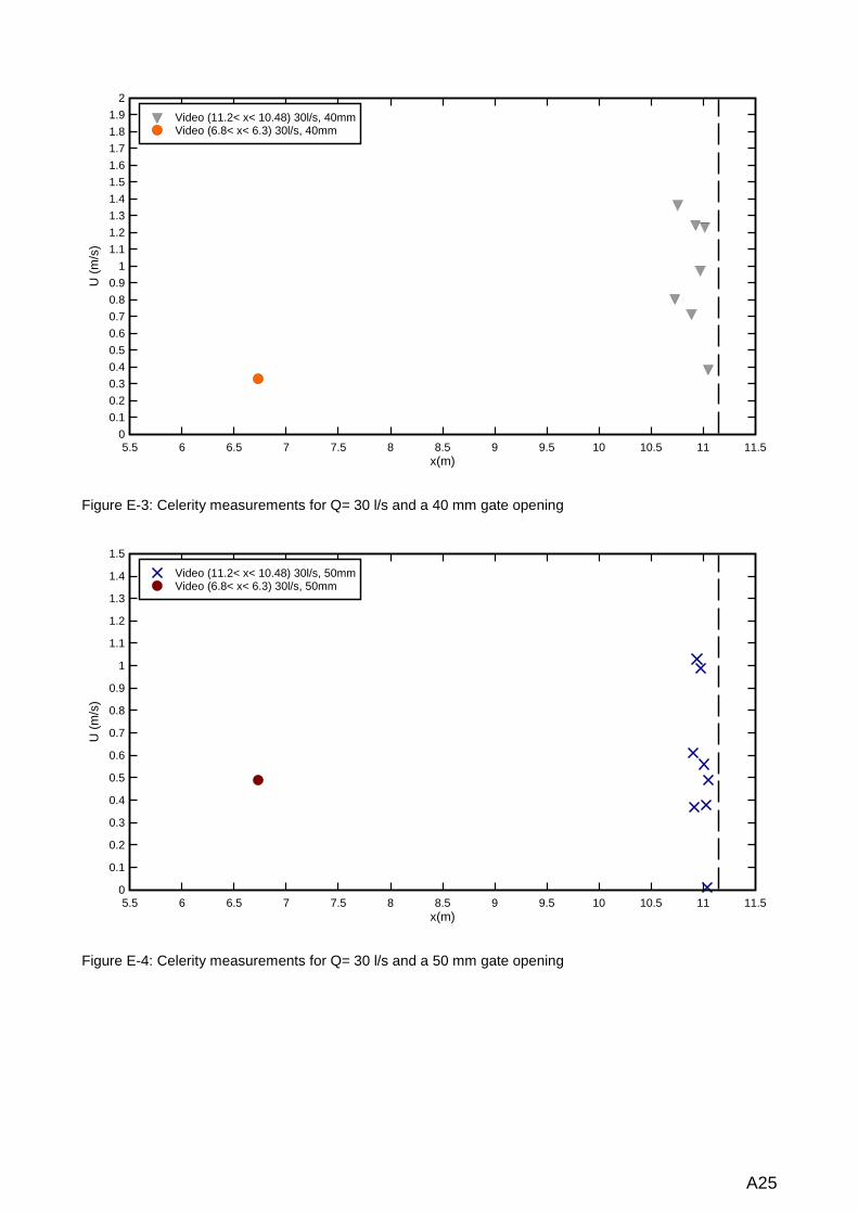
A25



x(m)

U (

m/s

)

5.5 6 6.5 7 7.5 8 8.5 9 9.5 10 10.5 11 11.50

0.1

0.2

0.3

0.4

0.5

0.6

0.7

0.8

0.9

1

1.1

1.2

1.3

1.4

1.5

1.6

1.7

1.8

1.9

2


x(m)

U (

m/s

)

5.5 6 6.5 7 7.5 8 8.5 9 9.5 10 10.5 11 11.50

0.1

0.2

0.3

0.4

0.5

0.6

0.7

0.8

0.9

1

1.1

1.2

1.3

1.4

1.5


A26

Appendix F – Steady state flow profiles

F-1 Presentation

The steady state flow profiles were recorded using ADM and video data. Typical steady

state flow profiles using acoustic displacement meters for the negative and positive surge

are illustrated in Figures F-1 and F-2 respectively. Typical steady state flow profiles using

video recordings for the positive and negative surge are illustrated in Figures F-3 and F-4

respectively.

Notations





F-2 Results

Figure F-1: Steady state profile for negative surge from ADM analysis, Q=20 l/s, h=30 mm, d0 at 6 m

Figure F-2: Steady state profile for positive surge from ADM analysis, Q=20 l/s, h=30 mm, d0 at 6 m

x (m)

d (c

m)

5.5 6 6.5 7 7.5 8 8.5 9 9.5 10 10.5 1121.3

21.4

21.5

21.6

21.7

21.8

21.9

22

22.1

22.2

22.3

22.4

x (m)

d (

cm

)

5.5 6 6.5 7 7.5 8 8.5 9 9.5 10 10.5 116.24

6.32

6.4

6.48

6.56

6.64

6.72

6.8

6.88

6.96

7.04

A27

Figure F-3: Dimensionless steady state profile positive surge from video data analysis

Figure F-4: Dimensionless steady state profile negative surge from video data analysis

x'/d0

d/d

' 0

0 0.5 1 1.5 2 2.5 3 3.5 4 4.5 5 5.5 6 6.5 7 7.5 8 8.5 90.9

0.93

0.96

0.99

1.02

1.05

1.08

1.11

1.14

1.17

1.2

Video (11.2< x <10.48), 20 l/s, 30mmVideo (11.2< x <10.48), 20 l/s, 50mm


x'/d0

d/d

' 0

0 0.25 0.5 0.75 1 1.25 1.5 1.75 2 2.25 2.5 2.750.9

0.91

0.92

0.93

0.94

0.95

0.96

0.97

0.98

0.99

1

1.01

1.02

1.03

1.04

1.05



hydraulic modelling of unsteady open channel flow ...263564/s42385743_mphil... · hydraulic...

Documents