hydraulics 3 gradually-varied flow - 1 dr david apsley 3

Hydraulics 3 Gradually-Varied Flow - 1 Dr David Apsley

3. GRADUALLY-VARIED FLOW (GVF) AUTUMN 2018 3.1 Normal Flow vs Gradually-Varied Flow

In normal flow the downslope component of weight balances bed friction. As a result, the

water depth h and velocity V are constant and the total-head line (or energy grade line) is

parallel to both the water surface and the channel bed; i.e. the friction slope Sf is the same as

the geometric slope S0.

As a result of disturbances due to hydraulic structures (weir, sluice, etc.) or changes to

channel width, slope or roughness the downslope component of weight may not locally

balance bed friction. As a result, the friction slope Sf and bed slope S0 will be different and

the water depth h and velocity V will change along the channel.

The gradually-varied-flow equation gives an expression for dh/dx and allows one to predict

the variation of water depth along the channel.

h

EGL (energy grade line)/2gV2

Friction slope Sf

Geometric slope S0

RVF GVF RVF GVF RVF GVF RVF GVF UF

sluicegate

hydraulicjump

weir changeof slope

GVF


3.2 Derivation of the Gradually-Varied-Flow Equation

Provided the pressure distribution is hydrostatic

then, at any streamwise location x:

The total head is

(1)

where zs is the level of the free surface and zb is the level of the bed.

Although not crucial, we make the small-slope assumption and make no distinction between

the vertical depth h (which forms part of the total head) and that perpendicular to the bed,

h cos θ (which is used to get the flow rate).

The total head may be written

(2)

where E is the specific energy, or head relative to the bed:

(3)

In frictionless flow, H = constant; i.e. the energy grade line is horizontal. In reality, H

decreases over large distances due to bed friction; the energy grade line slopes downward.

Differentiate (2):

(4)

Define:

(5)

(6)

Sf is the downward slope of the energy grade line, or friction slope; (more about how this is

calculated later). S0 is the actual geometric slope. Then

(7)

Thus, the specific energy only changes if there is a difference between the geometric and

friction slopes, i.e. between the rates at which gravity drives the flow and friction retards it.

Otherwise we would have normal flow, in which the depth and specific energy are constant.

Equations (5) and (7) are two forms of the gradually-varied-flow equation. However, the

third, and most common, form rewrites dE/dx in terms of the rate of change of depth, dh/dx.

h cos

gzs

zbh


bs

dh

A

(8)

where . Hence,

Differentiating with respect to streamwise distance x (using the chain rule for the last term):

If bs is the width of the channel at the surface:

and

Hence,

Combining this with (7) gives, finally,

Gradually-Varied-Flow Equation

(9)

3.3 Finding the Friction Slope

Since the flow (and hence the velocity profile and bed stress) vary only gradually with

distance, friction is primarily determined by the local bulk velocity V. The local friction slope

Sf can then be evaluated on the “quasi-uniform-flow” assumption that there is the same rate

of energy loss as in normal flow of the same depth; e.g. using Manning’s equation:

Inverting for the friction slope:

(10)

Both A and Rh (which depend on the channel shape) should be written in terms of depth h.

In general, the deeper the flow then the smaller the velocity and friction losses. Qualitatively,

greater depth lower velocity smaller Sf ;

smaller depth higher velocity greater Sf .


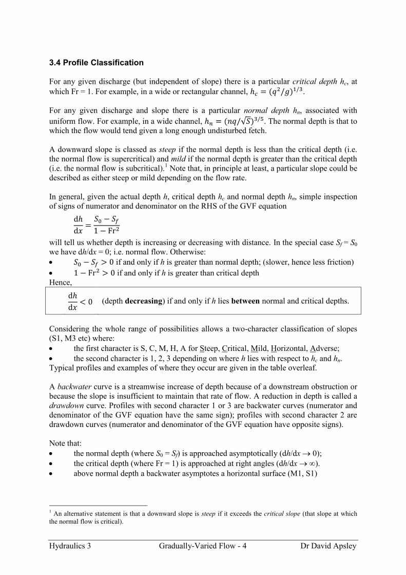
3.4 Profile Classification

For any given discharge (but independent of slope) there is a particular critical depth hc, at

which Fr = 1. For example, in a wide or rectangular channel, .

For any given discharge and slope there is a particular normal depth hn, associated with

uniform flow. For example, in a wide channel, . The normal depth is that to

which the flow would tend given a long enough undisturbed fetch.

A downward slope is classed as steep if the normal depth is less than the critical depth (i.e.

the normal flow is supercritical) and mild if the normal depth is greater than the critical depth

(i.e. the normal flow is subcritical).1 Note that, in principle at least, a particular slope could be

described as either steep or mild depending on the flow rate.

In general, given the actual depth h, critical depth hc and normal depth hn, simple inspection

of signs of numerator and denominator on the RHS of the GVF equation

will tell us whether depth is increasing or decreasing with distance. In the special case Sf = S0

we have dh/dx = 0; i.e. normal flow. Otherwise:

if and only if h is greater than normal depth; (slower, hence less friction)

if and only if h is greater than critical depth

Hence,

(depth decreasing) if and only if h lies between normal and critical depths.

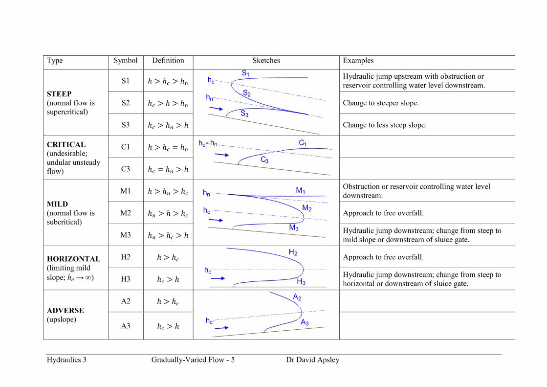
Considering the whole range of possibilities allows a two-character classification of slopes

(S1, M3 etc) where:

the first character is S, C, M, H, A for Steep, Critical, Mild, Horizontal, Adverse;

the second character is 1, 2, 3 depending on where h lies with respect to hc and hn.

Typical profiles and examples of where they occur are given in the table overleaf.

A backwater curve is a streamwise increase of depth because of a downstream obstruction or

because the slope is insufficient to maintain that rate of flow. A reduction in depth is called a

drawdown curve. Profiles with second character 1 or 3 are backwater curves (numerator and

denominator of the GVF equation have the same sign); profiles with second character 2 are

drawdown curves (numerator and denominator of the GVF equation have opposite signs).

Note that:

the normal depth (where S0 = Sf) is approached asymptotically (dh/dx 0);

the critical depth (where Fr = 1) is approached at right angles (dh/dx ).

above normal depth a backwater asymptotes a horizontal surface (M1, S1)

1 An alternative statement is that a downward slope is steep if it exceeds the critical slope (that slope at which

the normal flow is critical).


Type Symbol Definition Sketches Examples

STEEP

(normal flow is

supercritical)

S1

Hydraulic jump upstream with obstruction or

reservoir controlling water level downstream.

S2 Change to steeper slope.

S3 Change to less steep slope.

CRITICAL

(undesirable;

undular unsteady

flow)

C1

C3

MILD

(normal flow is

subcritical)

M1

Obstruction or reservoir controlling water level

downstream.

M2 Approach to free overfall.

M3 Hydraulic jump downstream; change from steep to

mild slope or downstream of sluice gate.

HORIZONTAL (limiting mild

slope; hn → )

H2

Approach to free overfall.

H3 Hydraulic jump downstream; change from steep to

horizontal or downstream of sluice gate.

ADVERSE (upslope)

A2

A3

hn

hc

S1

S2

S3

hnhc C1

3C

=

hn

hc

M1

M2

3M

H2

hc

3H

A2

hc 3A


3.5 Qualitative Examples of Open-Channel-Flow Behaviour

A control point is a location where there is a known relationship between water depth and

discharge (aka “stage-discharge relation”). Examples include critical-flow points (weirs,

venturi flumes, sudden changes in slope, free overfall), sluice gates, entry or discharge to a

reservoir. A hydraulic jump can also be classed as a control point. Control points often

provide a location where one can start a GVF calculation; i.e. a boundary condition.

Some general rules:

(i) Supercritical controlled by upstream conditions.

Subcritical controlled by downstream conditions.

(ii) Given a long-enough undisturbed fetch the flow will revert to normal flow.

(iii) A hydraulic jump occurs between regions of supercritical and subcritical gradually-

varied flow at the point where the jump condition for the sequent depths is correct.

(iv) Where the slope is mild (i.e. the normal flow is subcritical), and any downstream

control is a long way away, a hydraulic jump can be assumed to jump directly to the

normal depth.

Flow over a weir (mild slope)

Flow under a sluice gate – (a) mild slope

Flow under a sluice gate – (b) steep slope

WEIR

normal M1

normal

hydraulicjump

hnch

1h

2h M3

CP CP

hn

normal M1normal

hydraulicjump

hn

2h M3

CP CP

hn

h1

normalS1

2h S3

CP

nh

normal

nh

h1


Flow from a reservoir – (a) mild slope

Flow from a reservoir – (b) steep slope

Flow into a reservoir (mild slope)

Free overfall (mild slope)

RESERVOIR

hn

normalCP

RESERVOIR

hc

normal

S2

CP

RESERVOIR

hn

normalCPM1

hn

normal

CPM2

critical

hc


3.6 Numerical Solution of the GVF Equation

Analytical solutions of the GVF equation are very rare and it is usual to solve it numerically.

The process yields a series of discrete pairs of distance xi and depth hi. Intermediate points

can be determined, if required, by interpolation.

All methods employ a discrete approximation to one of the following forms of GVF equation:

(total head

) (11)

(specific energy

) (12)

(depth h) (13)

In any of these the friction slope can be obtained by inverting Manning’s equation:

(14)

and the Froude number is

(15)

where is the mean depth (= actual depth for a rectangular or wide channel).

Physically, integration should start at a control point and proceed:

forward in x if the flow is supercritical

(upstream control)

backward in x if the flow is subcritical

(downstream control).

There are two main classes of method:

Standard-step methods: solve for depth h at

specified distance intervals Δx.

Direct-step methods: solve for distance x at

specified depth intervals Δh. (One advantage is

that they can calculate profiles starting from a

critical point, where and standard-

step methods would fail).

0h h1

h2

h3

h4

x x x x

CPflow

CP

flow

x0 1x 2x 3x

h

h

h


3.6.1 Total-Head Form of the GVF Equation

This is solved as a standard-step method (find depth h at specified distance intervals Δx). The

equation is discretised as

(16)

solving sequentially for h1, h2, h3, … starting with the depth at the control point h0.

Since both H and Sf are functions of h, the method operates by adjusting hi+1 iteratively at

each step so that the LHS and RHS of (16) are equal.

This is a good method, but since it requires iterative solution at each step it is better suited to

a computer program than hand or spreadsheet calculation.

3.6.2 Specific-Energy Form of the GVF Equation

where

Since increments in E are determined by successive values of h, this is solved as a direct-step

method (find displacement x at specified depth intervals Δh).

First invert to make E the independent variable:

The equation is then discretised ( ) and rearranged for distance increments:

(17)

where

(18)

There are various ways of estimating the average slope difference. The example to follow

uses the average of values at depths hi and hi+1.


3.6.3 Depth Form of the GVF Equation

Here we shall solve this by a direct-step method (find displacement x at specified depth

intervals Δh).

First, invert to make h the independent variable:

The function on the RHS is first written as a function of h. The equation is then discretised

( ) and rearranged for distance increments as:

(19)

As before, the bracketed term on the RHS can be taken as the average of values at the start

and end of an interval or (my preference) by evaluation at the interval mid-depth:

Comment. Different authors adopt different ways of solving the GVF equation numerically,

particularly in choosing whether to use the specific-energy or depth form, and how to form

the average derivative (e.g., average of values at the ends of the interval or simply the single

value at the midpoint). All should give the same answer when the step size Δh becomes very

small, but may differ for the larger step sizes typical of hand calculations. The specific-

energy form seems to be slightly more common in the literature, but my own tests suggest

that the depth form, with derivative evaluated just once at the mid-point of the interval, gives

slightly better results for large step sizes. Note that surface profiles become highly curved

near critical points and more steps, with a smaller Δh, should be used there.


Example. (Exam 2007 – modified)

A long rectangular channel of width 4 m has a slope of 1:5000 and a Manning’s n of

0.015 m–1/3

s. The total discharge is 8 m3 s

–1. The channel narrows to a width of 1 m as a

venturi flume over a short length.

(a) Determine the normal depth for the 4 m wide channel.

(b) Show that critical conditions occur at the narrow 1 m wide section.

(c) Determine the depth just upstream of the venturi where the width is 4 m.

(d) Determine the distance upstream to where the depth is 5% greater than the normal

depth using two steps in the gradually-varied flow equation given below; (you may

use either form).

Data In standard notation,

or

Solution.

(a) For the normal depth,

where

,

Rearranging as an iterative formula for h to find the normal depth at the channel slope S0:

Here, with lengths in metres:

Iteration (from, e.g., h = 1.570) gives normal depth:

Answer: 2.09 m.

(b) To determine whether critical conditions occur, compare the total head in the approach

flow with that assuming critical conditions at the throat.

The total head, assuming normal flow and measuring heights from the bed of the channel is


At the throat the discharge per unit width is

The critical depth and critical specific energy at the throat are

Since the bed of the flume is flat (zb = 0), the critical head Hc = Ec.

Since the approach-flow head Ha is less than the critical head Hc (the minimum head required

to pass this flow rate through the venturi), the flow must back up and increase in depth just

upstream to supply this minimum head. It will then undergo a subcritical to supercritical

transition through the throat. The total head throughout the venturi is H = Hc = 2.804 m.

(c) In the vicinity of the venturi the total head is H = 2.804 m. Just upstream (where width

b = 4 m), we seek the subcritical solution of

Rearrange for the deeper solution:

Here, with lengths in metres:

Iterate (from, e.g., h = 2.804) to get the depth just upstream of the venturi:

Answer: 2.78 m

(d) Do a GVF calculation (subcritical, so physically it

should start at the fixed downstream control and work

upstream, although mathematically it can be done the other

way) from the pre-venturi depth (h = 2.778 m) to where

h = 2.194 m (i.e. 1.05hn). Using two steps the depth

increment per step is

x0x1x2

Step 1Step 2

h = 2.7780

h = 2.4861

h = 2.1942


Both depth and specific-energy methods are shown on the following pages.

METHOD 1: using the depth form of the GVF equation

(‘mid’ means mid-point of the interval: half way between hi and hi+1; sometimes written hi+½.)

For convenience, work out numerical expressions for Fr2 and Sf in terms of h:

Manning’s equation (see earlier) gave

Assuming that the rate of loss of energy (Sf) at a general depth h is the same as the channel

slope that would give normal flow at that depth, rearrangement for the slope gives

Hence,

With

and Δh = –0.292 m

working may then be set out in tabular form. (All depths assumed to be in metres.)

i hi xi hmid (dx/dh)mid Δx

0 2.778 0

2.632 10810 –3157

1 2.486 –3157

2.340 18850 –5504

2 2.194 –8661

This gives a distance of about 8.7 km upstream.


METHOD 2: Using the specific-energy form of the GVF equation

(‘av’ is taken as the average of values calculated at start and end of each interval in h.)

Here:

and the same expression as before may be used for Sf, so that:

With

working may then be set out in tabular form. (All depths assumed to be in metres.)

i hi xi Ei S0 –Sf ΔE (S0 –Sf)av Δx

0 2.778 0 2.804 1.04610–4

–0.285 8.88310–5

–3208

1 2.486 –3208 2.519 7.30410–5

–0.283 4.85110–5

–5834

2 2.194 –9042 2.236 2.39710–5

This gives a distance of about 9.0 km upstream.

Smaller steps Δh will give more accurate results (and closer agreement between the two

methods).


Example. (Exam 2008 – reworded)

A long, wide channel has a slope of 1:2747 with a Manning’s n of 0.015 m–1/3

s. It carries a

discharge of 2.5 m3 s

–1 per metre width, and there is a free overfall at the downstream end.

An undershot sluice is placed a certain distance upstream of the free overfall which

determines the nature of the flow between sluice and overfall. The depth just downstream of

the sluice is 0.5 m.

(a) Determine the critical depth and normal depth.

(b) Sketch, with explanation, the two possible gradually-varied flows between sluice and

overfall.

(c) Calculate the particular distance between sluice and overfall which determines the

boundary between these two flows. Use one step in the gradually-varied-flow

equation.

Example. (Exam 2018)

An undershot sluice controls the flow in a long rectangular channel of width 2.5 m,

Manning’s roughness coefficient n = 0.012 m–1/3

s and streamwise slope 0.002. The depths of

parallel flow upstream and downstream of the gate are 1.8 m and 0.3 m, respectively.

(a) Assuming no losses at the sluice, find the volume flow rate, Q.

(b) Find the normal and critical depths in the channel.

(c) Compute the distance from the sluice gate to the hydraulic jump, assuming normal

depth downstream of the jump. Use two steps in the gradually-varied-flow equation.

Example. (Exam 2014)

An undershot sluice is used to control the flow of water in a long wide channel of slope 0.003

and Manning’s roughness coefficient 0.012 m–1/3

s. The flow rate in the channel is 2 m3 s

–1

per metre width.

(a) Calculate the normal depth and critical depth in the channel and show that the channel

is hydrodynamically “steep” at this flow rate.

(b) The depth of flow just downstream of the sluice is 0.4 m. Assuming no head losses at

the sluice calculate the depth just upstream of the sluice.

(c) Sketch the depth profile along the channel, indicating clearly any flow transitions

brought about by the sluice and indicating where water depth is increasing or

decreasing.

(d) Use 2 steps in the gradually-varied flow equation to determine how far upstream of

the sluice a hydraulic jump will occur.

hydraulics 3 gradually-varied flow - 1 dr david apsley 3

Documents