hydraulique `a surface libre td2: numerical integration...
TRANSCRIPT
Hydraulique a surface libreTD2: Numerical integration, discretization
and schemes for solving differentialequations
Professor: C. AnceyTeaching assistant: T. Trewhela
ENAC / LHE - 2020
Outline
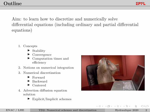
Aim: to learn how to discretize and numerically solvedifferential equations (including ordinary and partial differentialequations)
1. ConceptsI StabilityI ConvergenceI Computation times and
efficiency2. Notions on numerical integration3. Numerical discretization
I ForwardI BackwardI Centered
4. Advection diffusion equationsolution
I Explicit/Implicit schemes
ENAC / LHE TD2: Numerical schemes and discretization Hydraulique 2020 2
Stability
A numerical solution is called stable when numerical errors donot increase in the course of the numerical computation. Foriterative methods, a stable method is one for which the errorsdo not diverge to a point that they would be no longer bounded.
We will address stability in each problem we solve during thissession, and it is an important issue to address every time onesolve an equation numerically.
ENAC / LHE TD2: Numerical schemes and discretization Hydraulique 2020 3
Convergence
A numerical solution converges when the found solution tendsto the exact solution as the grid size tends to 0.
When the exact solution is unknown, the convergence must beproven with various solutions using different grid sizes. If thesolutions tend to fixed values and are consistent, then thesolution converges.
In all the exercises, convergence must be verified.
ENAC / LHE TD2: Numerical schemes and discretization Hydraulique 2020 4
Computation time and efficiency
Some numerical methods takemore time than others. Thereare several ways to improvecomputational times, such asvectorization for example.
In Matlab, it is highly advised to vectorize and avoid the usageof for/while cycles. Computational time can be evaluated usingthe tic/toc commands.
ENAC / LHE TD2: Numerical schemes and discretization Hydraulique 2020 5
Notions on numerical integration
a b
f(x)
x
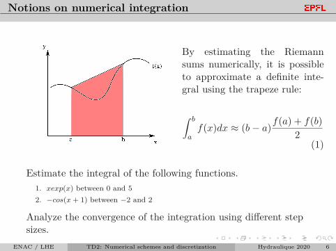
y By estimating the Riemannsums numerically, it is possibleto approximate a definite inte-gral using the trapeze rule:
∫ b
af(x)dx ≈ (b− a)f(a) + f(b)
2(1)
Estimate the integral of the following functions.1. xexp(x) between 0 and 52. −cos(x+ 1) between −2 and 2
Analyze the convergence of the integration using different stepsizes.
ENAC / LHE TD2: Numerical schemes and discretization Hydraulique 2020 6
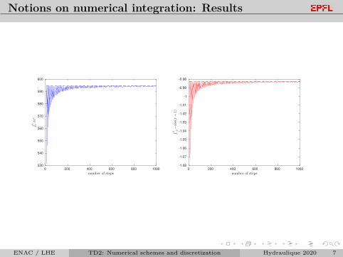
Notions on numerical integration: Results
0 200 400 600 800 1000
530
540
550
560
570
580
590
600
0 200 400 600 800 1000
-1.08
-1.07
-1.06
-1.05
-1.04
-1.03
-1.02
-1.01
-1
-0.99
-0.98
ENAC / LHE TD2: Numerical schemes and discretization Hydraulique 2020 7
Method for differential equations: Runge-Kutta 4
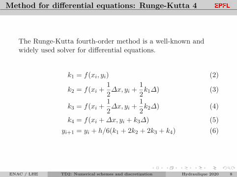
The Runge-Kutta fourth-order method is a well-known andwidely used solver for differential equations.
k1 = f(xi, yi) (2)
k2 = f(xi + 12∆x, yi + 1
2k1∆) (3)
k3 = f(xi + 12∆x, yi + 1
2k2∆) (4)
k4 = f(xi +∆x, yi + k3∆) (5)yi+1 = yi + h/6(k1 + 2k2 + 2k3 + k4) (6)
ENAC / LHE TD2: Numerical schemes and discretization Hydraulique 2020 8
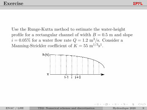
Exercise
Use the Runge-Kutta method to estimate the water-heightprofile for a rectangular channel of width B = 0.5 m and slopei = 0.05% for a water flow rate Q = 1.2 m3/s. Consider aManning-Strickler coefficient of K = 55 m1/3s1.
ENAC / LHE TD2: Numerical schemes and discretization Hydraulique 2020 9
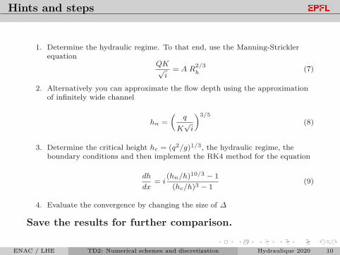
Hints and steps
1. Determine the hydraulic regime. To that end, use the Manning-Stricklerequation
QK√i
= A R2/3h
(7)
2. Alternatively you can approximate the flow depth using the approximationof infinitely wide channel
hn =(
q
K√i
)3/5(8)
3. Determine the critical height hc = (q2/g)1/3, the hydraulic regime, theboundary conditions and then implement the RK4 method for the equation
dh
dx= i
(hn/h)10/3 − 1(hc/h)3 − 1
(9)
4. Evaluate the convergence by changing the size of ∆
Save the results for further comparison.
ENAC / LHE TD2: Numerical schemes and discretization Hydraulique 2020 10
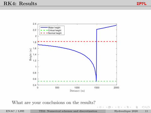
RK4: Results
0 500 1000 1500 20000.4
0.6
0.8
1
1.2
1.4
1.6
1.8
2
2.2
2.4
Water height
Critical height
Normal height
What are your conclusions on the results?
ENAC / LHE TD2: Numerical schemes and discretization Hydraulique 2020 11
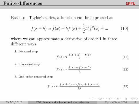
Finite differences
Based on Taylor’s series, a function can be expressed as
f(x+ h) ≈ f(x) + hf ′(x) + 12h
2f ′′(x) + ... (10)
where we can approximate a derivative of order 1 in threedifferent ways
1. Forward step
f ′(x) ≈f(x+ h)− f(x)
h(11)
2. Backward step
f ′(x) ≈f(x)− f(x− h)
h(12)
3. 2nd order centered step
f ′(x) ≈f(x+ h)− 2f(x) + f(x− h)
h2 (13)
ENAC / LHE TD2: Numerical schemes and discretization Hydraulique 2020 12
Optional exercise
Solve the water-height profile using a forward and a centeredscheme. What are the differences?
ENAC / LHE TD2: Numerical schemes and discretization Hydraulique 2020 13
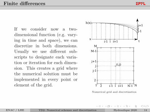
Finite differences
If we consider now a two-dimensional function (e.g. vary-ing in time and space), we candiscretize in both dimensions.Usually we use different sub-scripts to designate each varia-tion or iteration for each dimen-sion. This creates a grid wherethe numerical solution must beimplemented in every point orelement of the grid.
h(x)
xi i+1i-1 t
jj+1
j-1
1 N
M
2
2
N-1
M-1
(i,j)
i i+1i-1
j
j+1
j-1
Numerical grid and discretization
ENAC / LHE TD2: Numerical schemes and discretization Hydraulique 2020 14
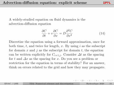
Advection-diffusion equation: explicit scheme
A widely-studied equation on fluid dynamics is theadvection-diffusion equation
∂C
∂t+ v
∂C
∂x= D
∂2C
∂x2 (14)
Discretize the equation using a forward approximation, once forboth time, t, and twice for length, x. By using i as the subscriptfor domain x and j as the subscript for domain t, the equationcan be written explicitly for Ci+1,j . Consider ∆t as the spacingfor t and ∆x as the spacing for x. Do you see a problem orrestriction for the equation in terms of stability? For an answer,think on errors related to the grid and how they may propagate.
ENAC / LHE TD2: Numerical schemes and discretization Hydraulique 2020 15
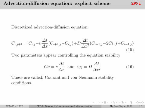
Advection-diffusion equation: explicit scheme
Discretized advection-diffusion equation
Ci,j+1 = Ci,j−v∆t
∆x(Ci+1,j−Ci,j)+D
∆t
∆x2 (Ci+1,j−2Ci, j+Ci−1,j)(15)
Two parameters appear controlling the equation stability
Co = v∆t
∆xand vN = D
∆t
∆x2 (16)
These are called, Courant and von Neumann stabilityconditions.
ENAC / LHE TD2: Numerical schemes and discretization Hydraulique 2020 16
Advection-diffusion equation: explicit scheme
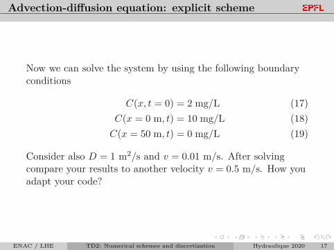
Now we can solve the system by using the following boundaryconditions
C(x, t = 0) = 2 mg/L (17)C(x = 0 m, t) = 10 mg/L (18)C(x = 50 m, t) = 0 mg/L (19)
Consider also D = 1 m2/s and v = 0.01 m/s. After solvingcompare your results to another velocity v = 0.5 m/s. How youadapt your code?
ENAC / LHE TD2: Numerical schemes and discretization Hydraulique 2020 17
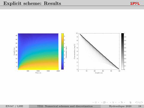
Explicit scheme: Results
500 1000 1500 2000
5
10
15
20
25
30
35
40
45
1
2
3
4
5
6
7
8
9
Concentr
ation (
mg/L
)
0 10 20 30 40 50
0
1
2
3
4
5
6
7
8
9
10
0
0.1
0.2
0.3
0.4
0.5
0.6
0.7
0.8
0.9
1
ENAC / LHE TD2: Numerical schemes and discretization Hydraulique 2020 18
Advection-diffusion equation: implicit scheme
An alternative is to write the advection-diffusion equation usingbackward finite differences.Rewrite the equation using backward finite differences for bothtime and space. What is the difference from the previous case?Solve your equations using the same conditions as for theexplicit scheme. Hint: Write your problem in matrix form.Compare your results to the previous scheme in terms ofstability, calculation time. What do you think about thesealternatives?
ENAC / LHE TD2: Numerical schemes and discretization Hydraulique 2020 19
Advection-diffusion equation: implicit scheme
The implicit scheme can be expressed as
Ci,j − Ci,j−1∆t
= −v ∆t∆x
(Ci+1,j−Ci,j)+D∆t
∆x2 (Ci+1,j−2Ci, j+Ci−1,j)(20)
which can be rewritten in matrix form
ACj = Cj−1 (21)
where Ai,i = 1 + 2vN + Co and Ai,i1 = Ai,i+1 = vN + Co. Don’tforget the boundary conditions!
ENAC / LHE TD2: Numerical schemes and discretization Hydraulique 2020 20