hydroclimate of the spring mountains and sheep … of the spring mountains and sheep range, clark...
TRANSCRIPT

Prepared in cooperation with the U.S. Forest Service, Bureau of Land Management, and U.S. Fish and Wildlife Service
Hydroclimate of the Spring Mountains and Sheep Range, Clark County, Nevada
U.S. Department of the InteriorU.S. Geological Survey
Scientific Investigations Report 2014–5142

Cover: Photograph showing part of the Spring Mountains including Charleston Peak, Joshua trees (Yucca brevifolia) in the foreground. Photograph taken by Michael T. Moreo, U.S. Geological Survey, February 2009.

Hydroclimate of the Spring Mountains and Sheep Range, Clark County, Nevada
By Michael T. Moreo, Gabriel B. Senay, Alan L. Flint, Nancy A. Damar, Randell J. Laczniak, and James Hurja
Prepared in cooperation with the U.S. Forest Service, Bureau of Land Management, and U.S. Fish and Wildlife Service
Scientific Investigations Report 2014–5142
U.S. Department of the InteriorU.S. Geological Survey

U.S. Department of the InteriorSALLY JEWELL, Secretary
U.S. Geological SurveySuzette M. Kimball, Acting Director
U.S. Geological Survey, Reston, Virginia: 2014
For more information on the USGS—the Federal source for science about the Earth, its natural and living resources, natural hazards, and the environment, visit http://www.usgs.gov or call 1–888–ASK–USGS.
For an overview of USGS information products, including maps, imagery, and publications, visit http://www.usgs.gov/pubprod
To order this and other USGS information products, visit http://store.usgs.gov
Any use of trade, firm, or product names is for descriptive purposes only and does not imply endorsement by the U.S. Government.
Although this information product, for the most part, is in the public domain, it also may contain copyrighted materials as noted in the text. Permission to reproduce copyrighted items must be secured from the copyright owner.
Suggested citation:Moreo, M.T., Senay, G.B., Flint, A.L., Damar, N.A., Laczniak, R.J., and Hurja, James, 2014, Hydroclimate of the Spring Mountains and Sheep Range, Clark County, Nevada: U.S. Geological Survey Scientific Investigations Report 2014–5142, 38 p., http://dx.doi.org/10.3133/sir20145142.
ISSN 2328-0328 (online)

iii
Contents
Abstract ...........................................................................................................................................................1Introduction.....................................................................................................................................................1
Purpose and Scope ..............................................................................................................................3Description of Study Area ...................................................................................................................3
Study Models ..................................................................................................................................................6Precipitation...........................................................................................................................................6Evapotranspiration................................................................................................................................6
Potential Evapotranspiration .....................................................................................................6Actual Evapotranspiration ..........................................................................................................6
Operational Simplified Surface Energy Balance Model ..............................................7Vegetation Evapotranspiration Model .............................................................................7
Hydroclimate of the Spring Mountains and Sheep Range .....................................................................8Precipitation Estimates ........................................................................................................................8Evapotranspiration Estimates ...........................................................................................................13Ecosystem Relations and Climatic Water Deficit ..........................................................................19Climate Zones and Aridity Index ......................................................................................................22Water Balance Estimates ..................................................................................................................22
Summary........................................................................................................................................................26References Cited..........................................................................................................................................26Appendix A. Geospatial Database, Spring Mountains and Sheep Range, Clark County, Nevada 31Appendix B. Evapotranspiration Data, Spring Mountains and Sheep Range, Clark County,
Nevada .............................................................................................................................................32Appendix C. Evaluation of Over-Estimation of Actual Evapotranspiration by the Operational
Simplified Surface Energy Balance Model in High-Elevation Areas, Spring Mountains and Sheep Range, Clark County, Nevada ...................................................................................33

iv
Figures 1. Map showing study area extent, Spring Mountains and Sheep Range, Clark County,
Nevada ...........................................................................................................................................2 2. Map showing ecosystem distribution and location of Soil Climate Analysis Network
(SCAN) and Snowpack Telemetry (SNOTEL) stations, Spring Mountains and Sheep Range, Clark County, Nevada .....................................................................................................5
3. Map showing distribution of mean annual (1971–2007) Parameter-elevation Regressions on Independent Slopes Model (PRISM) precipitation and location of U.S. Geological Survey high-elevation precipitation (HEP) gages, Spring Mountains and Sheep Range, Clark County, Nevada. ...............................................................................9
4. Graphs showing comparisons between annual Parameter-elevation Regressions on Independent Slopes Model (PRISM) precipitation and annual precipitation measured at five U.S. Geological Survey high-elevation precipitation gages, water years 1971–2007, Spring Mountains and Sheep Range, Clark County, Nevada ...............11
5. Graphs showing intra-annual pattern of mean monthly (1971–2007) Parameter-elevation Regressions on Independent Slopes Model (PRISM) precipitation, Spring Mountains and Sheep Range, Clark County, Nevada .....................12
6. Graph showing relation between mean annual Parameter-elevation Regressions on Independent Slopes Model (PRISM) precipitation and elevation, Spring Mountains and Sheep Range, Clark County, Nevada ...........................................................12
7. Map showing distribution of mean annual (1971–2007) Basin Characterization Model potential evapotranspiration (PET), Spring Mountains and Sheep Range, Clark County, Nevada .................................................................................................................14
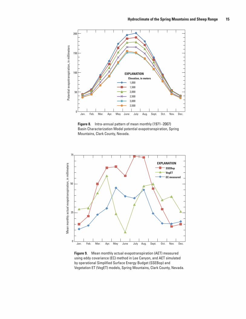
8. Graph showing intra-annual pattern of mean monthly (1971–2007) Basin Characterization Model potential evapotranspiration, Spring Mountains, Clark County, Nevada ...........................................................................................................................15
9. Graph showing mean monthly actual evapotranspiration (AET) measured using eddy covariance (EC) method in Lee Canyon, and AET simulated by operational Simplified Surface Energy Budget (SSEBop) and Vegetation ET (VegET) models, Spring Mountains, Clark County, Nevada ...............................................................................15
10. Graphs showing operational Simplified Surface Energy Budget (SSEBop) and Vegetation Evapotranspiration (VegET) actual evapotranspiration (AET), and Parameter-elevation Regressions on Independent Slopes Model (PRISM) precipitation (PPT) versus elevation, Spring Mountains and Sheep Range, Clark County, Nevada ...........................................................................................................................16
11. Map showing distribution of mean annual (2001–11) Vegetation Evapotranspiration model actual evapotranspiration, Spring Mountains and Sheep Range, Clark County, Nevada ...........................................................................................................................18
12. Graphs showing relations between mean ecosystem elevations and mean annual precipitation and actual evapotranspiration, and potential evapotranspiration and climatic water deficit, Spring Mountains and Sheep Range, Clark County, Nevada ......20

v
Figures—Continued 13. Map showing distribution of mean annual climatic water deficit, Spring Mountains
and Sheep Range, Clark County, Nevada ...............................................................................21 14. Map showing distribution of mean annual (1971–2007) aridity index and climate
zones, Spring Mountains and Sheep Range, Clark County, Nevada .................................23 15. Graphs showing intra-annual patterns of mean monthly precipitation and snow depth
measured at the Lee Canyon Snowpack Telemetry (SNOTEL) station, and volumetric soil water content (SWC) and actual evapotranspiration (AET) measured at Lee Canyon SNOTEL and eddy-covariance (EC) stations, July 2008 through June 2010, Spring Mountains, Clark County, Nevada ...............................................................................24
16. Graph showing recharge efficiency as a function of elevation, Spring Mountains and Sheep Range, Clark County, Nevada ...............................................................................25
Tables 1. Elevation and summary statistics for U.S. Geological Survey (USGS) high-elevation
precipitation gages, water years 1986–2007, Spring Mountains and Sheep Range, Clark County, Nevada .................................................................................................................13
2. Monthly actual evapotranspiration (AET) data and statistics from eddy-covariance station, Lee Canyon, Spring Mountains, Clark County, Nevada, July 4, 2008–April 7, 2011 ...............................................................................................................................................16
3. Correlative analyses of mean annual hydroclimatic variables and mean ecosystem elevations, Spring Mountains and Sheep Range, Clark County, Nevada .........................19
4. Mean annual ecosystem water budgets and hydroclimate data, Spring Mountains and Sheep Range, Clark County, Nevada ...............................................................................22

vi
Conversion Factors and Datums
Conversion Factors
SI to Inch/Pound
Multiply By To obtain
Length
centimeter (cm) 0.3937 inch (in.)millimeter (mm) 0.03937 inch (in.)meter (m) 3.281 foot (ft) kilometer (km) 0.6214 mile (mi)
Area
square meter (m2) 0.0002471 acre square kilometer (km2) 0.3861 square mile (mi2)square kilometer (km2) 247.1044 acre
Volume
cubic meter (m3) 0.0002642 million gallons (Mgal) cubic meter (m3) 0.0008107 acre-foot (acre-ft) million cubic meter (Mm3) 0.8107132 thousand acre-foot (Kaf)
Flow rate
meter per second (m/s) 2.2369 miles per hour (mi/h) millimeter per year (mm/yr) 0.03937 inch per year (in/yr)
Mass
gram (g) 0.03527 ounce, avoirdupois (oz)
Pressure
kilopascal (kPa) 0.1450 pound per square inch (lb/in2)
Density
gram per cubic meter (g/m3) 0.00006242 pound per cubic foot (lb/ft3)
Energy
watt per square meter (W/m2) 0.0222 calorie per second per square foot [(cal/s)/ft2]
Temperature in degrees Celsius (°C) may be converted to degrees Fahrenheit (°F) as follows:
°F = (1.8 ×°C) + 32
Temperature in degrees Celsius (°C) may be converted to kelvins (K) as follows:
[ ]°C°C
1KK= +273.15
1
Datums
Vertical coordinate information is referenced to North American Vertical Datum of 1988 (NAVD 88).
Horizontal coordinate information is referenced to North American Datum of 1983 (NAD 83).
Elevation, as used in this report, refers to distance above the vertical datum.

Hydroclimate of the Spring Mountains and Sheep Range, Clark County, Nevada
By Michael T. Moreo1, Gabriel B. Senay1, Alan L. Flint1, Nancy A. Damar1, Randell J. Laczniak1, and James Hurja2
AbstractPrecipitation, potential evapotranspiration, and actual
evapotranspiration often are used to characterize the hydroclimate of a region. Quantification of these parameters in mountainous terrains is difficult because limited access often hampers the collection of representative ground data. To fulfill a need to characterize ecological zones in the Spring Mountains and Sheep Range of southern Nevada, spatially and temporally explicit estimates of these hydroclimatic parameters are determined from remote-sensing and model-based methodologies. Parameter-elevation Regressions on Independent Slopes Model (PRISM) precipitation estimates for this area ranges from about 100 millimeters (mm) in the low elevations of the study area (700 meters [m]) to more than 700 mm in the high elevations of the Spring Mountains (> 2,800 m). The PRISM model underestimates precipitation by 7–15 percent based on a comparison with four high-elevation precipitation gages having more than 20 years of record. Precipitation at 3,000-m elevation is 50 percent greater in the Spring Mountains than in the Sheep Range. The lesser amount of precipitation in the Sheep Range is attributed to partial moisture depletion by the Spring Mountains of eastward-moving, cool-season (October–April) storms. Cool-season storms account for 66–76 percent of annual precipitation. Potential evapotranspiration estimates by the Basin Characterization Model range from about 700 mm in the high elevations of the Spring Mountains to 1,600 mm in the low elevations of the study area. The model realistically simulates lower potential evapotranspiration on northeast-to-northwest facing slopes compared to adjacent southeast-to-southwest facing slopes. Actual evapotranspiration, estimated using a Moderate Resolution Imaging Spectroradiometer based water-balance model, ranges from about 100 to 600 mm. The magnitude and spatial variation of simulated, actual evapotranspiration was validated by comparison to
PRISM precipitation. Estimated groundwater recharge, computed as the residual of precipitation depleted by actual evapotranspiration, is within the range of previous estimates. A climatic water deficit dataset and aridity-index-based climate zones are derived from precipitation and evapotranspiration datasets. Climate zones range from arid in the lower elevations of the study area to humid in small pockets on north- to northeast-facing slopes in the high elevations of the Spring Mountains. Correlative analyses between hydroclimatic variables and mean ecosystem elevations indicate that the climatic water deficit is the best predictor of ecosystem distribution (R2 = 0.92). Computed water balances indicate that substantially more recharge is generated in the Spring Mountains than in the Sheep Range. A geospatial database containing compiled and developed hydroclimatic data and other pertinent information accompanies this report.
IntroductionThe U.S. Forest Service (USFS), Bureau of Land
Management, and U.S. Fish and Wildlife Service are conducting a study to characterize ecological zones in the Spring Mountains and Sheep Range in southern Nevada (fig. 1). The Spring Mountains and Sheep Range are home to some of the most isolated and biologically diverse species and vegetative communities in the Mojave Desert. High- elevation communities, often referred to as “sky islands,” are particularly susceptible to the effects of climate change and harbor more than 41 percent of the endemic species in the Mojave Desert Ecoregion (The Nature Conservancy, 2001; Randall and others, 2010). Because hydroclimatic data are sparse in this area of high topoclimatic variability, USFS and other land-management agencies lack sufficient information to understand the relation between hydroclimatic variables and the distribution and productivity of ecological zones, or how ecological zones may be affected by climate change.
1U.S. Geological Survey.2U.S. Forest Service.

2 Hydroclimate of the Spring Mountains and Sheep Range, Clark County, Nevada
sac14-4204_fig 01
SP
RI N
G M
OU
NT
AI N
S
SH
EE
P
RA
NG
E
Study Area
CL
AR
K
CLARK
LINCOLN
Charleston Peak
Hayford Peak
Las Vegas ValleyLakeMead
Pahrump ValleyNEVADA
CALIFORNIA
NY
E
INYO
SANTA BARBARA
NEVADA UTAH
ARIZONA
CALIFORNIA
LasVegas
Study area
EXPLANATIONStudy area boundary
115°115°30'116°
37°
36°30'
36°
0 10 20 30 40 MILES
0 10 20 30 40 KILOMETERS
Base from ESRI ArcGIS Online Services, ESRI Imagery World 2D layer accessed November 2013; U.S. Census Bureau TIGER/Line 2010: U.S. Geological Survey 2012Spatial reference system: UniversalTransverse Mercator projection, Zone 11,North American Datum of 1983
ARIZONA
Figure 1. Study area extent, Spring Mountains and Sheep Range, Clark County, Nevada.

Introduction 3
Ecological zones are large areas with similar environmental conditions, which are manifested by characteristic vegetative communities (Simon and others, 2005). The U.S. Geological Survey (USGS), as part of this comprehensive study, is characterizing the local hydroclimate emphasizing the magnitude, timing, and distribution of precipitation and evapotranspiration. Concurrently, the Natural Resources Conservation Service (NRCS) is conducting detailed soil surveys. Additionally, NRCS and USFS have established Snowpack Telemetry (SNOTEL), Soil Climate Analysis Network (SCAN), and other micrometeorological stations in a general transect from the Spring Mountains to the Sheep Range to collect long-term climate data. Previous studies have focused primarily on understanding the occurrence and distribution of vegetative communities (Clark County, 2000; Prior-Magee and others, 2007; Heaton and others, 2011).
A thorough knowledge of local hydrologic processes is vital to understanding the occurrence of ecological zones and the populations, communities, and ecosystems within them. Water availability is critical to all living organisms and all water available to terrestrial ecosystems is provided by the atmospheric output of moisture in the form of solid and liquid precipitation. Terrestrial moisture is converted to the vapor phase by irradiant energy and returned to the atmosphere through evaporation and transpiration processes, known collectively as evapotranspiration. A relatively small amount of precipitation falling at high elevations infiltrates the soil, percolates past root zones, and recharges the underlying aquifers. Precipitation stored in upper soil layers becomes available for uptake by the local vegetation provided the water potential in the soil is higher than in the plant roots. The flux and storage of water are poorly understood in the study area. The relation between precipitation and evapotranspiration is the fundamental climatic influence driving multiple processes at the land-atmosphere interface (Shelton, 2009).
Quantifying the magnitude of precipitation and evapotranspiration, and their spatial and temporal distributions, is within the realm of hydroclimatology. Hydroclimatology couples the traditional sciences of hydrology and climatology to account for energy and moisture exchanges between the Earth’s surface and atmosphere. At the global scale, differential heating of the Earth’s surface results in energy and moisture imbalances that create atmospheric pressure gradients that form the systematic framework of global air transport. Local-scale vertical fluxes of energy and moisture at the Earth’s surface are superimposed on these global circulation patterns. The hydroclimate of any specified area is defined by these global- and local-scale thermodynamic and hydrodynamic processes that drive energy and moisture exchanges at the land-atmosphere interface. Quantifying these hydroclimatic processes characterized by precipitation-evapotranspiration fluxes and resulting storages is a prerequisite to developing a water balance that can be used for subsequent interdisciplinary studies (Shelton, 2009).
Purpose and Scope
This report documents the hydroclimate of the Spring Mountains and Sheep Range in southern Nevada emphasizing the magnitude, timing, and distribution of precipitation and evapotranspiration. Spatially explicit estimates of precipitation, potential evapotranspiration (PET), and actual evapotranspiration (AET) are developed from mathematical models that represent the physical processes occurring in the study area. The remote-sensing and model-based methodology of this research is necessitated by the challenges posed by limited accessibility and sparse data in the mountainous terrain of the study area; although limited, ground measurements are used to validate the accuracy of model simulations to the extent possible. Maps are presented that illustrate precipitation, PET, AET, and derivative products in time and space. Spatiotemporal relations between hydroclimatic variables, elevation gradients, and vegetation-based ecosystem distributions are explored.
This report and the accompanying geospatial database (appendix A) are expected to provide a baseline hydroclimatic framework from which ecological zones will be delineated and characterized. The geospatial database contains pertinent geospatial data including simulated mean annual precipitation, PET, and AET distributions. A more thorough understanding of the relation between the hydroclimate, geology, soils, and vegetation distributions will help land managers evaluate and characterize present-day conditions, and will provide a basis for predicting ecological-zone response to natural or anthropogenic forces such as climate change. Moreover, the data generated from this research effort also can be used to support future biophysical and water-availability impact studies, including ecophysiological, climate change, and groundwater recharge modeling efforts.
Description of Study Area
The major topographic features of the 6,350 km2 study area are the Spring Mountains and Sheep Range (fig. 1). Located in the Basin and Range Physiographic Province, these mountain ranges primarily consist of exposed Paleozoic limestone and are flanked by extensive alluvial fans. The valley floor separating the two ranges consists of thick Cenozoic basin-fill deposits that overlie the Las Vegas Valley shear zone—a right-lateral, strike-slip fault with 50 km of displacement (Page and others, 2005). The steep topography characterizing the study area exhibits about 3 km of relief. The highest points are Charleston Peak (3,652 m) in the Spring Mountains and Hayford Peak (3,021 m) in the Sheep Range. Charleston Peak is the highest point in the Mojave Desert.

4 Hydroclimate of the Spring Mountains and Sheep Range, Clark County, Nevada
The geographic setting, topographic relief, and atmospheric circulation patterns are the primary hydroclimatic controls in the study area. The location of the study area relative to the Pacific Ocean is such that a substantial amount of moisture from prevailing westerly winter storms is captured by orographic lifting associated with the intervening Sierra Nevada Mountains. This capture, or “rain shadow,” results in leeward storms of diminished moisture content. Nevertheless, these areally extensive low-pressure, low-intensity winter storms account for two-thirds to three-quarters of mean annual precipitation. Despite its close proximity to the Pacific Ocean, the clear dry air of the study area attributed to the rain shadow effect results in large diurnal temperature fluctuations that are more continental than maritime in nature. During summer months, monsoonal air flow from the south accounts for high-intensity, short-duration convective storms of limited areal extent. Mean annual precipitation ranges from about 100 mm at low elevations (700 m) to more than 700 mm at high elevations (> 2,800 m). Temperature decreases and precipitation increases, with increasing elevation, result in a markedly colder and wetter climate than the desert conditions more common at low elevations. The dominant presence of the Spring Mountain and Sheep Range creates a highly complex hydroclimatic pattern that supports a rich and diverse flora (Houghton and others, 1975).
Groundwater recharge processes begin at high elevations in the Spring Mountains and Sheep Range. Annual precipitation is highest during the winter when PET and air temperatures are at their annual minima resulting in snow accumulations. Precipitation decreases during the spring as PET and air temperatures increase resulting in snowmelt and increasing AET. Snowmelt infiltrates the surface and increases the soil moisture. When soil water storage exceeds capacity, recharge is generated and percolation through the underlying bedrock proceeds at a rate determined by the hydraulic conductivity. Percolating subsurface water is captured as recharge to local perched aquifers; is intercepted and discharged at local springs; or travels through the highly-fractured Paleozoic carbonate rock to replenish regional aquifers that often extend laterally into and beyond adjacent valleys. Surface runoff is generally short-lived and considered negligible for water balance calculations. Minimal or no recharge occurs in warmer, low-elevation areas where PET is greater and precipitation is substantially less than at high elevations. Water recharged in the Spring Mountains, and to a lesser extent the Sheep Range, is the primary source of groundwater for Las Vegas Valley, Pahrump Valley, and the springs discharging to the Ash Meadows National Wildlife Refuge (AMNWR) located about 27 km west of the northwestern part of the study area boundary (San Juan and others, 2010). AMNWR is home to the highest concentration of endemic species in the United States harboring nearly 30 endemic species (7 listed as threatened and 5 listed as endangered) including the Devils Hole pupfish (Cyprinodon diabolis) (U.S. Fish and Wildlife Service, 2013). Recharge
processes in the Great Basin region are well documented in Harrill and Prudic (1998), Stonestrom and others (2007), and Flint and Flint (2007a).
Vegetation assemblages in Clark County, Nevada, have been organized into communities and ecosystems based on similar characteristics for management purposes. The vegetation-based ecosystem distribution shown in figure 2 was produced for the Clark County Multiple Species Habitat Conservation Program (Heaton and others, 2011), and represents a refinement of previous classification efforts (Clark County, 2000). Ecosystems occurring in the study area are:
• Alpine—distribution limited to only 1.2 km2 above 3,500 m elevation in the Spring Mountains,
• Bristlecone pine—ranging in elevation from 2,700 to 3,500 m in the Spring Mountains and Sheep Range,
• Mixed conifer—ranging in elevation from 2,200 to 3,300 m in the Spring Mountains and Sheep Range,
• Pinion-juniper—ranging in elevation from 1,500 to 2,500 m in the Spring Mountains and Sheep Range,
• Sagebrush—ranging in elevation from 1,500 to 2,800 m in the Spring Mountains and Sheep Range,
• Blackbrush—below 1,800 m in elevation,• Salt desert scrub—ranging in elevation from 1,000
to 1,800 m, • Mojave Desert scrub—below 1,200 m in elevation,• Mesquite-acacia—occurs near springs, on sandy
hummocks, and in washes within Mohave Desert scrub and salt desert scrub ecosystems, and
• Disturbed—areas within ecosystems with some degree of human management.
The need for long-term climate data has been recognized, and as part of this study nine permanent climate and soil monitoring stations were installed and will be maintained by NRCS—six SCAN stations (data can be accessed at http://www.wcc.nrcs.usda.gov/scan/Nevada/nevada.html) and three SNOTEL stations (data can be accessed at http://www.wcc.nrcs.usda.gov/snotel/Nevada/nevada.html) (fig. 2). SCAN sites measure liquid precipitation, air temperature, relative humidity, barometric pressure, wind speed and direction, solar radiation, soil moisture, and soil temperature. The SNOTEL sites measure liquid and solid precipitation, air temperature, snow water content, snow depth, wind speed and direction, solar radiation, soil moisture, and soil temperature. SCAN and SNOTEL stations were augmented for this project with a net radiometer to measure the energy balance between the incoming and outgoing shortwave and longwave radiation. These sites should provide valuable data that will support future modeling efforts undertaken to better understand ecological zones and environmental processes in the study area.

Introduction 5
sac14-4204_fig 02
2,000
2,000
3,000
2,000
1,0001,000
1,00
01,
000
2,000
2,000
2,00
02,
000
1,0001,000
1,00
01,
000
NEVADACALIFORNIA
LINCOLN
NY
E
INYO
PahrumpValley
Las VegasValley
CLARK
CL
AR
K
CharlestonPeak
HayfordPeak
SP
RI N
G M
OU
NT
AI N
S
SH
EE
P
RA
NG
E
99
11
44
6655
88
77
22
33
Ecosystems from Heaton and others (2011) D21 final
SCANSNOTEL
EXPLANATIONEcosystem
Station type, name andnumber on map
Alpine
Bristlecone pine
Mixed conifer
Pinion-juniper
Blackbrush
Sagebrush
Mojave Desert scrub
Salt desert scrub
Mesquite-acacia
1 Charkiln2 Trough Springs3 Bristlecone Trail4 Lee Canyon5 Kyle Canyon6 Rainbow Canyon7 Lovell Summit8 Hayford Peak9 Pine Nut
Disturbed
0 10 20 MILES
0 10 20 KILOMETERS
Study area boundary
Elevation, in meters above the North American Vertical Datum of 1988
1,000
36°30'
36°
115°115°30'116°
Shaded-relief base from 10-meter National Elevation Data, 2011. Spatial reference system: UniversalTransverse Mercator projection, Zone 11, North American Datum of 1983
Figure 2. Ecosystem distribution and location of Soil Climate Analysis Network (SCAN) and Snowpack Telemetry (SNOTEL) stations, Spring Mountains and Sheep Range, Clark County, Nevada.

6 Hydroclimate of the Spring Mountains and Sheep Range, Clark County, Nevada
Study ModelsThis section describes the models used to develop
precipitation, PET, and AET estimates. Monthly outputs for each model are aggregated into mean water year (October–September) estimates.
Precipitation
Monthly Parameter-elevation Regressions on Independent Slopes Model (PRISM) 30-arcsec (about 800-m) grid resolution LT71m (LT, long term; m, monthly) time-series datasets were compiled and used to estimate mean annual precipitation (and minimum and maximum air temperatures) for water years 1971 through 2007 (PRISM Climate Group, 2008; Daly and others, 2008). The LT71m dataset is derived from station networks that include stations with more than 20 years of data for long-term consistency. Interpolation between stations is aided by using 1971–2000 long-term normals as predictor grids. The advantage of this climatologically aided interpolation (CAI) method is that the interpolator is robust to wide variations in station data density. Station data in southern Nevada is especially sparse compared to other parts of the United States.
Evapotranspiration
Estimating evapotranspiration in mountain environments is particularly problematic because spatial and topographic variations in precipitation and PET are considerable, and access to representative measurement sites is limited. PET is a measure of the evaporative power of the atmosphere and defines the amount of evapotranspiration that would occur assuming an unlimited water supply. The water supply at the land surface is determined by precipitation magnitude and timing. The primary climatic variables controlling PET are solar radiation, air temperature and humidity, and wind speed (Allen and others, 1998). Solar irradiation at the land surface is the primary source of available energy driving evapotranspiration processes. Available energy is related to PET through the Priestley-Taylor equation (Priestley and Taylor, 1972). Given a wet surface and air temperature near 24 °C, available energy is equal to both PET and AET (Flint and Childs, 1991). Greater water availability means a greater proportion of available energy is partitioned into latent-heat energy. Latent heat is the energy consumed converting water from a liquid or solid to vapor. Available energy is partitioned either into latent- or sensible-heat energy. A greater proportion of available energy is partitioned into sensible heat in dryer environments where water supplies are limited. Sensible heat is the movement of heat energy that results from a temperature difference between the surface and the atmosphere.
Latent- and sensible-heat energy fluxes are difficult to measure directly and any attempt to extrapolate point measurements in mountain environments are complicated by many factors including PET that varies with elevation and surface slope and aspect, and precipitation that varies with elevation and between adjacent mountain ranges. Models used to estimate evapotranspiration for this research effort are described in the following sections.
Potential EvapotranspirationFor this study, PET is estimated from Basin
Characterization Model (BCM) 270-m gridded datasets (Flint and Flint, 2007a; Thorne and others, 2012). Monthly datasets were compiled for water years 1971–2007. The BCM is a distributed-parameter, water-balance model that uses spatially distributed climate and physical properties, with mechanistic, process-based algebraic equations to perform water-balance calculations. The BCM relies on an hourly energy-balance subroutine that is based on solar radiation, air temperature, and the Priestley-Taylor equation (Priestley and Taylor, 1972; Flint and Childs, 1991) to calculate PET (Flint and Childs, 1987). Clear sky PET is calculated using a solar radiation model that incorporates seasonal atmospheric transmissivity parameters and site parameters of slope, aspect, and topographic shading (to define the percentage of sky seen for every grid cell) (Flint and Flint, 2007b). Hourly PET is aggregated into monthly estimates and corrected for local cloud cover using cloudiness data from National Renewable Energy Laboratory (NREL). Simulated PET for the southwestern United States is calibrated to measured PET from California Irrigation Management Information System and Arizona Meteorological Network stations (Flint and Flint, 2007a; Flint and others, 2012). All input data are downscaled or interpolated to the 270-m spatial resolution for model application following Flint and Flint (2012).
Actual EvapotranspirationFor this study, AET is estimated using two different
models that provide spatially explicit values. One, the Operational Simplified Surface Energy Balance (SSEBop) model, uses an energy balance approach; and the other, the Vegetation Evapotranspiration (VegET) model, uses a water balance approach. Both models use data acquired by a Moderate Resolution Imaging Spectroradiometer (MODIS) sensor aboard the Terra and Aqua satellites, which were launched in 1999 and 2002, respectively. The two modeling approaches require different input data to quantify the spatial variability of AET; the SSEBop model uses thermal data (with a spatial resolution of 1,000 m), whereas the VegET model uses Normalized Difference Vegetation Index (NDVI, 250 m spatial resolution) data computed from red and near-infrared

Study Models 7
bands of the electromagnetic spectrum. Both models use BCM PET data to define the upper limit of AET and output monthly AET datasets with spatial resolutions of 1,000 m (SSEBop) and 250 m (VegET).
Operational Simplified Surface Energy Balance ModelThe SSEBop model primarily uses land-surface
temperature (LST) and PET data (Senay and others, 2013) to compute AET. The model starts with a surface energy balance for a potential condition (assuming full vegetation cover and unlimited water supply) using PET as AET. Evapotranspiration fractions (ETf) account for differences in water availability across the landscape, and are used to adjust the PET based on a pixel’s LST value in relation to the “hot” and “cold” boundary reference conditions (equation 1). LST data are derived from 8-day average MODIS dataset with a 1,000-m spatial resolution.
The formulation of the SSEBop model is an adaptation of the “hot and cold” pixel approach from the Surface Energy Balance Algorithm for Land (SEBAL) model of Bastiaanssen and others (1998) and Mapping Evapotranspiration at High Resolution and Internalized Calibration (METRIC) of Allen and others (2007). In principle, instantaneous LST at satellite overpass time can be used to identify hot and cold pixels which in turn can be used to calculate ETf on a per pixel basis. This approach works well in a region with uniform hydroclimatic conditions such as irrigated basins. In order to eliminate the manual selection of hot and cold reference pixels, which also introduces subjective errors, SSEBop pre-defines the hot and cold boundary conditions specific to a given location and period using a combination of air temperature and clear-sky energy balance calculations (Senay and others, 2013).
The dimensionless ETf is calculated for each pixel by applying the following equation to each 8-day LST grid:
ETfTh TsdT
=− (1)
where ETf is the evapotranspiration fraction (0–1), Ts is the surface temperature, derived from
MODIS LST or Landsat thermal data, dT is a pre-defined (from the clear-sky radiation
balance calculation) temperature difference between the hot and cold reference boundary conditions that are unique for each day and pixel, ranging generally between 5 kelvin (K) and 25 K depending on location and season, and
Th is the hot reference boundary condition, representing the temperature of a dry-bare (hot) surface:
Th Tc dT= + (2)
where Tc is the cold boundary condition, representing
the cold- and wet-vegetated surface that is in equilibrium with the air temperature (all net radiation is used for latent-heat flux).
Tc is estimated by linearly disaggregating monthly PRISM maximum air temperature data for the given 8-day period. A correction coefficient of 0.985 is necessary to adjust for use of the maximum air temperature as a surrogate for the LST of well-watered vegetation at the time of satellite overpass, which occurs at a nominal overpass time of 10:30 a.m. (Pacific Standard Time). This implies that 98.5 percent of the maximum air temperature is considered as the cold/wet boundary condition at which LST AET is expected to equal PET. It is important that the cold boundary condition (Tc) is an accurate representation of the real value because a direct bias could be introduced owing to an over- or underestimation error. For example, during the growing season where the dT (Th – Tc) is about 20 K, an overestimation of Tc by 5 K could increase the ETf of a pixel by 0.25, which could be an increase of 50 percent if the true ETf of the pixel is only 0.5, that is, ETf changes from 0.5 to 0.75. Such errors have a potential to occur in topographically complex regions where simulated air temperature datasets must be interpolated from sparse station data.
Knowing ETf , AET is computed as:
AET ET PET= ×f (3)
where simulated PET is obtained from the BCM (Flint and Flint, 2007a). Monthly PET values were disaggregated into 8-day time periods assuming a linear distribution in the month to match the 8-day LST datasets. Because PET datasets were only available through water year 2007, the median of water years 2001–07 was calculated for each 8-day period to be used for water years 2008–09. Although the use of the median PET data will reduce some year-to-year variability, the spatial variability in AET is considerably more sensitive to the variability in the LST than to the variability in the PET.
Vegetation Evapotranspiration ModelThe VegET model simulates soil water levels in the root
zone (to 1 m depth below the surface) through a daily water balance algorithm that estimates AET in precipitation-driven landscapes (Senay, 2008). For this study, the key input data to the VegET model are PRISM precipitation, BCM PET, soil water holding capacity (WHC), and land surface phenology (LSP)-based crop coefficient (Kcp). AET is calculated as the product of PET, soil stress coefficient (Ks), and Kcp:

8 Hydroclimate of the Spring Mountains and Sheep Range, Clark County, Nevada
AET PET= × ×Kcp Ks (4)
where Kcp is LSP-based crop coefficient (ratio: 0.2–1.3),
and Ks is soil water stress coefficient (ratio: 0.0–1.0).
Ks is determined from a soil water balance model similar to procedures described in Allen and others (1998) and the gridded version developed by Senay and Verdin (2003) using equation 5. The dimensionless Ks coefficient varies from 0.0 to 1.0 depending on the soil water level in the modeling unit:
KsSWMAD
SW MAD K SW MADii S i= < = ≥, ; . ,1 0 (5)
where SWi is the soil water level of current time step, in
millimeters (equation 6), and MAD is the maximum allowable depletion level of
soil water in the root zone, in millimeters.
When MAD is less than SWi, AET is constrained by the availability of soil water and will be less than the potential. Although MAD varies by crop/vegetation type, a nominal value of 50 percent of the soil WHC can be used for most generalized crops such as cereals and natural vegetation. Thus, MAD is estimated as 50 percent of the soil WHC. Soil WHC—computed as the difference between field capacity and permanent wilting point—is derived from the NRCS State Soil Geographic database (Soil Survey Staff, 2011).
SWi is determined using a daily soil water balance described in equation 6. AET is estimated iteratively from equations 5 and 6. The model estimates saturation excess (assumed percolation deeper than 1 m for this study) where soil water in excess of the WHC of the soil is considered to be unavailable for plant use in the root zone; thus SWi is reset to a maximum of WHC or a minimum of 0.0 at the end of time step “i”:
SW SW PPTi i i i= + −−1 AET (6)
where SWi is level of soil water (soil moisture in depth
unit) at current model time step, in millimeters,
SWi-1 is level of soil water at previous model time step, in millimeters,
PPTi is precipitation during current model time step, in millimeters, and
AETi is actual evapotranspiration during current model time step, in millimeters.
Finally, to solve equation 4, the LSP-based crop coefficient Kcp is calculated using NDVI as shown in equation 7 which is formulated from an equation developed by Choudhury and others (1994) and confirmed by Tasumi and Allen (2007) for use with a grass-reference PET:
Kcp = +1 25 0 2. .NDVI (7)
where NDVI is the 8-day composite calculated from the 16-day, 250-m resolution MODIS NDVI data obtained from NASA LP DAAC (https://lpdaac.usgs.gov/get_data) with a linear interpolation in time. PRISM precipitation data were available only through water year 2007, and therefore, the median precipitation value of water years 2001–07 was calculated for each 8-day period and used for water years 2008–11. Owing to the limited number of years, the median was selected instead of the mean to minimize the influence of large deviations in a given year that may distort the climatology. Year-to-year precipitation variability in the Kcp was accounted for indirectly by the unique 8-day NDVI. A more detailed description of the setup and initialization of the VegET model is given in Senay and Verdin (2003) and Senay (2008).
Hydroclimate of the Spring Mountains and Sheep Range
Simulated, spatially explicit estimates of precipitation, PET, and AET are described and evaluated in this section. The accuracy of model-simulated estimates is validated with limited ground measurements to the extent possible. The hydroclimatic variables compiled and calculated for this study are assigned and summarized by ecosystem to explore the spatial variability and relations between these variables, elevation, and ecosystem distribution. Aridity-index-based climate zones and climatic water deficit datasets are calculated from precipitation and evapotranspiration datasets. Site- and ecosystem-scale water balances are computed. A geospatial database (appendix A) suitable for ecological zone characterization analyses is developed from hydroclimate estimates and other ancillary data.
Precipitation EstimatesThe accuracy of PRISM precipitation is validated by
comparison to available precipitation records. The distribution of mean annual precipitation estimated by PRISM for water years 1971–2007 is shown in figure 3. Mean annual precipitation ranges from 108 mm in the low elevations of the study area to more than 700 mm in the high elevations of the Spring Mountains. The lower PRISM precipitation bound of 108 mm is similar to mean annual precipitation of 105 mm measured at the Las Vegas airport (660 m elevation) from 1937 to 2013 (Western Region Climate Center, 2014).

Hydroclimate of the Spring Mountains and Sheep Range 9
sac14-4204_fig 03
2,000
2,000
3,000
2,000
1,0001,000
1,00
01,
000
2,000
2,000
2,000
2,000
1,0001,000
1,00
01,
000
NEVADACALIFORNIA
CLARK
CharlestonPeak
INYO
PahrumpValley
Las VegasValley
LINCOLN
NY
E
CLARK
SP
RI N
G M
OU
NT
AI N
S
SH
EE
P
RA
NG
EC
LA
RK
Sheep Peak
Lee Canyon
Kyle CanyonKyle Canyon
Hayford Peak
Trough Spring
Las Vegas
West ofcrest
East of crestEast of crest
West ofcrest
SHEEP RANGESHEEP RANGE
SPRINGMOUNTAINS
SPRINGMOUNTAINS
EXPLANATION
PRISM precipitation,in millimeters per year
768
108
200
300
400
500
600
700
0 10 20 MILES
0 10 20 KILOMETERS
USGS HEP gage
Study area boundary
Elevation, in meters above the North American Vertical Datum of 1988
1,000
36°30'
36°
115°115°30'116°
Shaded-relief base from 10-meter National Elevation Data, 2011. Spatial reference system: UniversalTransverse Mercator projection, Zone 11, North American Datum of 1983
Parameter-elevation on Independent Slopes Model (PRISM)PRISM Climate Group, Oregon State University
Created July, 2008
Figure 3. Distribution of mean annual (1971–2007) Parameter-elevation Regressions on Independent Slopes Model (PRISM) precipitation and location of U.S. Geological Survey high-elevation precipitation (HEP) gages, Spring Mountains and Sheep Range, Clark County, Nevada. Inset shows study area subdivisions used for analyses.

10 Hydroclimate of the Spring Mountains and Sheep Range, Clark County, Nevada
Additional validation data are provided by five gages located in the current study area from a USGS high-elevation precipitation (HEP) network (fig. 3). Each shielded gage is 3-m in height and 0.3-m in diameter. Data are typically collected during May and October of each year, and are not corrected for wind-induced catch deficiencies (Larsen and Peck, 1974). Wind speed and temperature data are not measured at orifice height; therefore, the magnitudes of these deficiencies are not known. Years having only partial data are excluded from the analysis. HEP gage elevations and summary statistics from water years 1986–2007 are given in table 1 (data can be accessed at http://waterdata.usgs.gov/nv/nwis/). Linear correlations between PRISM and measured precipitation are strong. Coefficients of determination (R2) range from 0.62 to 0.81 (fig. 4). Generally, PRISM precipitation underestimates measured precipitation for above-average years and overestimates for below-average years. Mean PRISM precipitation ranges from 7 to 15 percent less than the measured mean at all sites except Trough Springs where the simulated mean is 10 percent greater than the measured mean. The difference between the simulated and measured means at the Trough Springs gage may be related to the steep local topography near the site and the relatively coarse PRISM grid. PRISM precipitation is 10 percent less just 1,200 m southwest and downslope of the gage. The intra-annual pattern of mean monthly PRISM precipitation is shown in figure 5. About 37 percent of annual PRISM precipitation occurs from January through March, whereas only about 13 percent occurs from April through June. The proportion of cool season (October–April) to annual precipitation estimated by PRISM (69 percent) is within the range of cool season precipitation measured at the HEP gages (66–76 percent). Precipitation measured at the USGS HEP network compares favorably with precipitation measured annually at another high-elevation network maintained by the Nevada Division of Water Resources (NDWR, data can be accessed at http://water.nv.gov/data/precipitation/index.cfm; Fenelon and Moreo, 2002). The NDWR network is a precipitation data source used in the development of the PRISM 1971–2000 normal dataset (Norm71m) that in turn is used in the CAI process to develop the LT71m datasets used for this study (http://prism.oregonstate.edu/documents/PRISM_datasets_aug2013.pdf).
Mean annual PRISM precipitation was plotted at 10-m elevation increments beginning at 1,000 m to evaluate the relation between precipitation and elevation within and between the two mountain ranges. For this analysis, the study area was subdivided into (1) two sections so that the Spring Mountains could be considered separately from Sheep Range, and (2) four sections with each mountain range divided along its crest to separate east- and west-trending slopes so that
differences between windward and leeward slopes could be evaluated separately (fig. 3 inset). Each pixel in the mean annual PRISM precipitation grid was assigned an elevation using a 30-m digital elevation model. The elevation of each pixel was then rounded to the nearest 10-m increment and the mean precipitation value computed. Resulting precipitation-elevation plots of all data for each range indicate that precipitation increases with elevation in both ranges but that the rate of increase is greater in the Spring Mountains than in the Sheep Range (fig. 6). Precipitation in both ranges is similar at 1,000 m. At 2,000 and 3,000 m, precipitation in the Spring Mountains is 32 and 50 percent greater than in the Sheep Range, respectively.
The most likely explanation for this difference is a local rain shadow effect caused by the Spring Mountains on the Sheep Range during the cool season when winter storms bring moisture in from the Pacific. Quiring (1965) suggested that the relatively high elevation of the Spring Mountains and Sheep Range can be expected to produce variations in the local precipitation, but that it is unlikely this influence would be noticeable over a substantial area as is the case with the Sierra Nevada Mountains. Ralph and others (2003) found evidence of local rain shadow effects on adjacent watersheds in the Santa Cruz area of California. However, data do not indicate a rain shadow effect on leeward versus windward slopes. A double-tailed, paired t-test (assuming unequal variances) was conducted at the α = 0.05 probability level to determine whether precipitation estimated for windward (western) and leeward (eastern) slopes of each range are statistically different from each other. Differences are not significant in the Spring Mountains (n = 247, t-stat = 0.0014, p = 0.999, east of crest mean = 417, west of crest mean = 417) and Sheep Range (n = 195, t-stat = 0.6088, p = 0.543, east of crest mean = 276, west of crest mean = 272). The reason for the absence of a rain shadow here may be explained by the local topography in relation to storm directions. Quiring (1965) reported that low-pressure systems develop (cyclogenesis) with significant frequency in southern Nevada during the winter. Cyclogenesis draws additional moisture from the south and results in secondary storm tracks from the southwest. These secondary storm tracks result in a greater amount of moisture depletion northward in the Spring Mountains. This finding is supported by precipitation data from the HEP gages in the Spring Mountains. Precipitation amounts decrease from the southernmost (Kyle Canyon) to northernmost (Trough Spring) gages even though gage elevations are similar (fig. 3, table 1). Simulated mean annual PRISM precipitation data are included in the geospatial database (appendix A).

Hydroclimate of the Spring Mountains and Sheep Range 11
Figure 4. Comparisons between annual Parameter-elevation Regressions on Independent Slopes Model (PRISM) precipitation and annual precipitation measured at five U.S. Geological Survey high-elevation precipitation gages, water years 1971–2007, Spring Mountains and Sheep Range, Clark County, Nevada.
sac14-4204_fig04
0
500
1,000
1,500
PRIS
M p
reci
pita
tion,
in m
illim
eter
s PR
ISM
pre
cipi
tatio
n, in
mill
imet
ers
PRIS
M p
reci
pita
tion,
in m
illim
eter
s
PRIS
M p
reci
pita
tion,
in m
illim
eter
s PR
ISM
pre
cipi
tatio
n, in
mill
imet
ers
0
250
500
750
1,000
0
250
500
750
1,000
0 500 1,000 1,500
Measured precipitation, in millimeters
0 250 500 750 1,000
Measured precipitation, in millimeters
0 250 500 750 1,000
Measured precipitation, in millimeters
0 250 500 750 1,000
Measured precipitation, in millimeters
0 250 500 750 1,000
Measured precipitation, in millimeters
0
250
500
750
1,000
0
250
500
750
1,000
Mean annualmeasuredprecipitation(630)
Mean annualmeasuredprecipitation(418)
Mean annualmeasuredprecipitation(396)
Mean annualmeasuredprecipitation(362)
Mean annualmeasuredprecipitation(530)
Kyle Canyon, Spring Mountains Lee Canyon, Spring Mountains
Trough Springs, Spring Mountains
Sheep Peak, Sheep Range Hayford Peak, Sheep Range
R² = 0.77
1:1 LINE
1:1 LINE
1:1 LINE 1:1 LINE
R² = 0.62
1:1 LINE
R² = 0.76
R² = 0.81
R² = 0.74

12 Hydroclimate of the Spring Mountains and Sheep Range, Clark County, Nevada
sac14-4204_fig05
0
25
50
75
100
PRIS
M p
reci
pita
tion,
in m
illim
eter
s 3,000
2,500
2,000
1,500
1,000
Sheep Range
0
25
50
75
100
Jan. Feb. Mar. Apr. May June July Aug. Sept. Oct. Nov. Dec. Jan. Feb. Mar. Apr. May June July Aug. Sept. Oct. Nov. Dec.
PRIS
M p
reci
pita
tion,
in m
illim
eter
s
3,500
3,000
2,500
2,000
1,500
1,000
Spring Mountains
EXPLANATION EXPLANATIONElevation, in meters Elevation, in meters
Figure 5. Intra-annual pattern of mean monthly (1971–2007) Parameter-elevation Regressions on Independent Slopes Model (PRISM) precipitation, Spring Mountains and Sheep Range, Clark County, Nevada.
sac14-4204_fig06
y = 0.20x - 23.82 R ² = 0.97
y = 0.13x + 27.55 R ² = 0.97
0
250
500
750
0 1,000 2,000 3,000 4,000
PRIS
M p
reci
pita
tion,
in m
illim
eter
s
Elevation, in meters
Spring Mountains
Sheep Range
EXPLANATION
Figure 6. Graph showing relation between mean annual Parameter-elevation Regressions on Independent Slopes Model (PRISM) precipitation and elevation, Spring Mountains and Sheep Range, Clark County, Nevada.

Hydroclimate of the Spring Mountains and Sheep Range 13
Table 1. Elevation and summary statistics for U.S. Geological Survey (USGS) high-elevation precipitation gages, water years 1986–2007, Spring Mountains and Sheep Range, Clark County, Nevada.
Elevation and summary statistics (USGS site identification)
Kyle Canyon (361457115373301)
Lee Canyon (361822115402501)
Trough Spring (362240115462101)
Sheep Peak (363500115144301)
Hayford Peak (363929115115801)
Number of water years 22 19 18 16 20Mean, in millimeters 630 530 418 362 396Median, in millimeters 613 533 349 333 330Standard deviation, in millimeters 301 136 185 205 202Elevation, in meters 2,565 2,594 2,512 2,926 2,999
Evapotranspiration Estimates
The distribution of mean annual PET estimated by the BCM is shown in figure 7. Results range from about 700 mm in the high elevations of the Spring Mountains to about 1,600 mm in the low elevations of the study area. PET decreases by about 430 mm for each 1,000 m increase in elevation (lapse rate). Even though solar irradiance increases at higher elevations owing to a decrease in atmospheric diffusion, the air temperature lapse rate is the primary forcing mechanism. The lapse rate of air temperature in the study area averages about -0.01 °C/m, meaning air temperature decreases by an average of about 10 °C for each 1,000 m increase in elevation (appendix C). Within the local complexities of mountain topography, however, solar irradiance is the primary forcing mechanism. Mean annual PET on a south facing slope may be as much as 50 percent greater than on the adjacent north facing slope at the same elevation. Seasonally, differences are greater during winter than summer because the increasing solar zenith angle generally increases solar irradiance incident to south facing slopes; whereas, solar irradiance on north facing slopes decrease. The BCM realistically simulates differences on northeast-to-northwest facing slopes (lower PET) compared to southeast-to-southwest facing slopes (higher PET). The intra-annual pattern of mean monthly PET follows a typical mid-latitude, northern hemisphere, solar pattern with a peak in June–July and trough in December–January. Figure 8 shows this pattern for different elevations in the Spring Mountains. Simulated mean annual BCM PET data are included in the geospatial database (appendix A).
Mean monthly SSEBop and VegET simulated AET estimates are compared to AET measured at an eddy covariance (EC) station to evaluate the intra-annual pattern of simulated AET (fig. 9). The EC station was located at an elevation of 2,630 m in a ponderosa pine forest, within the mixed conifer ecosystem, approximately 50 m south of the Lee Canyon SNOTEL station (fig. 2). The period of operation was from July 4, 2008, to April 7, 2011. EC data filters, gap-filling, and corrections were applied following the procedures outlined in Moreo and others (2007). The
station was not in operation from February 10 to April 9, 2009. This period was not gap-filled, and these months are excluded from monthly statistics. For the rest of the record, 6.8 percent of data were filtered and gap-filled. The energy-balance ratio for the period of record was 0.74, indicating that 74 percent of measured available energy was accounted by measured turbulent energy (latent-heat plus sensible-heat energy fluxes). This energy imbalance was corrected and uncertainty computed as described in Moreo and Swancar (2013). Monthly AET data and statistics are given in table 2 (daily data are given in appendix B). Because the EC sensors were positioned only 4 m above the ground surface, AET measurements were sub-canopy. A tower constructed above the canopy was not possible because of scenic and wilderness area restrictions in much of the high elevation areas of the Spring Mountains. Understory vegetation in the EC source area was extremely sparse; therefore, measured AET represents sublimation and bare-ground evaporation processes, and little if any ponderosa pine transpiration. Accordingly, simulated AET, which does account for transpiration, is expected to be greater than measured AET. The mean annual sums are 318 mm measured by the EC station, 419 mm simulated by the VegET model, and 546 mm simulated by the SSEBop model. Despite the difference in magnitude, there is a good correlation (R2 = 0.82) between mean monthly measured AET and SSEBop AET; whereas, the correlation between measured AET and VegET AET is poor (R2 = 0.01). The correlation between SSEBop AET and mean monthly volumetric soil water content measured at a depth of 20 cm at the Lee Canyon SNOTEL station also is good (R2 = 0.84). However, the VegET magnitude (419 mm) compares favorably to measured AET (318 mm) plus growing season transpiration (117 mm) estimated for a mature ponderosa pine forest (Ryan and others, 2000). The comparisons of measured to simulated AET relied on only the single pixel where the EC station was located because there was minimal variation in simulated AET in the surrounding pixels.
The magnitude and spatial variation of simulated mean annual AET is compared to mean annual PRISM precipitation at 10-m elevation increments to further assess the accuracy of the SSEBop and VegET models (fig. 10).

14 Hydroclimate of the Spring Mountains and Sheep Range, Clark County, Nevada
sac14-4204_fig 07
2,000
2,000
3,000
2,000
1,0001,000
1,00
01,
000
2,000
2,000
2,00
02,
000
1,0001,000
1,00
01,
000
NEVADACALIFORNIA
LINCOLN
NY
E
INYO
PahrumpValley
Las VegasValley
HayfordPeak
CLARK
CL
AR
K
CharlestonPeak
SP
RI N
G M
OU
NT
AI N
S
SH
EE
P
RA
NG
E
EXPLANATIONPotential evapotranspiration,in millimeters per year
698
1,100
1,000
1,200
1,300
1,400
1,500
1,594
0 10 20 MILES
0 10 20 KILOMETERS
Study area boundary
Elevation, in meters above the North American Vertical Datum of 1988
1,000
36°30'
36°
115°115°30'116°
Shaded-relief base from 10-meter National Elevation Data, 2011. Spatial reference system: UniversalTransverse Mercator projection, Zone 11, North American Datum of 1983
Figure 7. Distribution of mean annual (1971–2007) Basin Characterization Model potential evapotranspiration (PET), Spring Mountains and Sheep Range, Clark County, Nevada.
Hydroclimate of the Spring Mountains and Sheep Range 15
sac14-4204_fig08
0
50
100
150
200
Jan. Feb. Mar. Apr. May June July Aug. Sept. Oct. Nov. Dec.
Pote
ntia
l eva
potra
nspi
ratio
n, in
mill
imet
ers
1,000
1,500
2,000
2,500
3,000
3,500
EXPLANATIONElevation, in meters
Figure 8. Intra-annual pattern of mean monthly (1971–2007) Basin Characterization Model potential evapotranspiration, Spring Mountains, Clark County, Nevada.
sac14-4204_fig09
0
25
50
75
Jan. Feb. Mar. Apr. May June July Aug. Sept. Oct. Nov. Dec.
Mea
n m
onth
ly a
ctua
l eva
potra
nspi
ratio
n, in
mill
imet
ers
SSEBop
VegET
EC measured
EXPLANATION
Figure 9. Mean monthly actual evapotranspiration (AET) measured using eddy covariance (EC) method in Lee Canyon, and AET simulated by operational Simplified Surface Energy Budget (SSEBop) and Vegetation ET (VegET) models, Spring Mountains, Clark County, Nevada.

16 Hydroclimate of the Spring Mountains and Sheep Range, Clark County, Nevada
Table 2. Monthly actual evapotranspiration (AET) data and statistics from eddy-covariance station, Lee Canyon, Spring Mountains, Clark County, Nevada, July 4, 2008–April 7, 2011.
[All values in millimeters unless otherwise noted]
MonthMinimum measured
AET
Maximum measured
AET
Mean measured AET
(not corrected for energy imbalance)
Number of months
in mean (n)
Mean measured AET (corrected for
energy imbalance)
Uncertainty of energy-balance corrected mean
AET
January 8 12 9 3 11 2February 9 15 12 2 14 2March 18 22 20 2 23 4April 24 24 24 1 29 4May 38 41 39 2 47 7June 32 35 33 2 39 6July 26 38 32 2 38 6August 30 48 38 3 45 7September 13 31 21 3 24 4October 5 19 13 3 16 2November 10 16 13 3 15 2December 10 17 15 3 17 3
sac14-4204_fig10
0
200
400
600
800
1,000
0 1,000 2,000 3,000 4,000
Shee
p Ra
nge
wat
er fl
ux, i
n m
illim
eter
s pe
r yea
r
Elevation, in meters
0
200
400
600
800
1,000
0 1,000 2,000 3,000 4,000
Sprin
g M
ount
ains
wat
er fl
ux, i
n m
illim
eter
s pe
r yea
r
Elevation, in meters
SSEBop AET
PRISM PPT
VegET AET
EXPLANATION
A B
Figure 10. Operational Simplified Surface Energy Budget (SSEBop) and Vegetation Evapotranspiration (VegET) actual evapotranspiration (AET), and Parameter-elevation Regressions on Independent Slopes Model (PRISM) precipitation (PPT) versus elevation, (A) Spring Mountains and (B) Sheep Range, Clark County, Nevada.

Hydroclimate of the Spring Mountains and Sheep Range 17
Despite the realistic pattern of simulated intra-annual AET and good correlation to soil moisture, SSEBop AET is substantially greater than PRISM precipitation at upper elevations. These results contradict the conceptual understanding of mountain recharge processes in that precipitation generally should be greater than AET in the high elevations of the Spring Mountains and Sheep Range. Conversely, VegET AET is consistent with hydrologic expectations. PRISM precipitation is similar to VegET AET at low elevations but exceeds VegET AET at high elevations. PRISM precipitation and VegET AET data are further compared using a two-sample t-test (assuming unequal variances) to determine whether differences between these two variables were significant at the α = 0.05 probability level. Differences are not significant below 2,000 m in the Spring Mountains (n = 129, t-stat = 0.23, p = 0.41, PRISM mean = 242, VegET mean = 239) and Sheep Range (n = 141, t-stat = -0.91, p = 0.18, PRISM mean = 196, VegET mean = 201). AET and precipitation measured at two low elevation sites using the Bowen ratio energy budget method validate this result (appendix B). However, differences are significant at elevations above 2,000 m in the Spring Mountains (n = 153, t-stat = 18.33, p < 0.01, PRISM mean = 535, VegET mean = 411) and Sheep Range (n = 99, t-stat = 11.89, p < 0.01, PRISM mean = 350, VegET mean = 319). The slope of precipitation-elevation relations flattens slightly above 2,000 m, whereas the slope of the AET-elevation relations level off or decreases. This result indicates that as the elevation increases, more water is increasingly available than can be evaporated and transpired; therefore, more water is increasingly available to recharge processes.
A mean annual water balance for the entire study area is computed to validate the magnitude of mean annual VegET AET. Regional groundwater recharge can be estimated by subtracting VegET AET from PRISM precipitation assuming that (1) runoff in the study area is minor, (2) PRISM-estimated precipitation is reasonably accurate, and (3) changes in soil moisture storage are negligible on a mean annual basis (Shelton, 2009). The computed recharge is 82 Mm3 (67 Kaf), which is 5.4 percent of the mean annual PRISM precipitation volume of 1,532 Mm3 (1,242 Kaf). This proportion of recharge is within the range of 0.3 to 6 percent of precipitation reported by Flint and Flint (2007a) for 194 basins in southwestern United States. Furthermore, this value is consistent with recharge previously reported by investigators using various methods. Water recharged in the Spring Mountains, and to a lesser extent the Sheep Range, is the primary source of groundwater replenishing aquifer systems beneath Las Vegas and Pahrump Valleys, and discharging to springs in the AMNWR. Previous estimates
of regional groundwater recharge to Las Vegas Valley ranges from 31 to 43 Mm3 (25–35 Kaf) (Maxey and Jameson, 1948; Malmberg, 1965; Harrill, 1976; Dettinger, 1989), to Pahrump Valley ranges from 27 to 32 Mm3 (22–26 Kaf) (Malmberg, 1967; Harrill, 1986), and to AMNWR springs ranges from 12 to 22 Mm3 (10–18 Kaf) (Walker and Eakin, 1963; Thomas and others, 1996; Belcher and Sweetkind, 2010). The total regional recharge computed for the current study of 82 Mm3 is within the range of 70 to 97 Mm3 estimated in previous studies.
Based on the preceding arguments, the distribution and magnitude of mean annual AET simulated by the VegET model are considered acceptable for the purpose and scope of this study. Simulated mean annual VegET AET data are included in the geospatial database (appendix A). Like PET, VegET AET rates are high on southeast-to-southwest facing slopes, and low on northeast-to-northwest facing slopes (fig. 11). Precipitation being equivalent, low simulated AET on northeast-to-northwest facing slopes results in higher recharge than on southeast-to-southwest facing slopes. The VegET model performed well at the annual timescale because precipitation-driven AET is the dominant process both physically and in the model. However, the VegET model does not adequately simulate the intra-annual pattern of AET at higher elevations primarily because the one-dimensional soil-water simulation in the root-zone does not account for the time lag between snowfall and snowmelt, which results in an overestimation of AET from autumn through early spring and an underestimation from early spring through autumn.
Additional research is required to improve both models in performance and usability in similar natural environments. The weak performance (overestimation) of the SSEBop model at higher elevations at the annual timescale can largely be attributed to a combination of model assumptions and input data errors. Particularly, the model is sensitive to the air temperature dataset that forms the basis for the cold boundary condition. An investigation of the air temperature dataset indicated a smaller lapse rate (for example, -0.0074 K/m) than the lapse rate obtained from the LST (-0.01 K/m). This resulted in a relatively high air temperature in the high elevation areas (compared to the changes in LST), which leads to an overestimation of the ETf and thus the AET. Additional information regarding SSEBop overestimation of AET is available in appendix C. The VegET model has shown reasonably good performance in precipitation-driven systems (Senay, 2008, and as shown in this study); the good performance of the model at an annual timescale points to the possibility of integrating the VegET model with a two-dimensional snowmelt and transport model to improve its intra-annual performance in similar environments.

18 Hydroclimate of the Spring Mountains and Sheep Range, Clark County, Nevada
sac14-4204_fig 11
2,000
2,000
3,000
2,000
1,0001,000
1,00
01,
000
2,000
2,000
2,00
02,
000
1,0001,000
1,00
01,
000
NEVADACALIFORNIA
LINCOLN
NY
E
INYO
PahrumpValley
HayfordPeak
Las VegasValley
CLARK
CL
AR
K
CharlestonPeak
SP
RI N
G M
OU
NT
AI N
S
SH
EE
P
RA
NG
EEXPLANATION
122
300
200
400
500
611
Actual evapotranspiration,in millimeters per year
0 10 20 MILES
0 10 20 KILOMETERS
Study area boundary
Elevation, in meters above the North American Vertical Datum of 1988
1,000
36°30'
36°
115°115°30'116°
Shaded-relief base from 10-meter National Elevation Data, 2011. Spatial reference system: UniversalTransverse Mercator projection, Zone 11, North American Datum of 1983
Figure 11. Distribution of mean annual (2001–11) Vegetation Evapotranspiration model actual evapotranspiration, Spring Mountains and Sheep Range, Clark County, Nevada.

Hydroclimate of the Spring Mountains and Sheep Range 19
Ecosystem Relations and Climatic Water Deficit
The hydroclimatic variables compiled and calculated for this study are summarized by ecosystem to explore the spatial variability and general relations between these variables, elevation, and ecosystem distribution. More detailed ecosystem analyses are beyond the scope of the current study. The study area is subdivided into five sections with each mountain range divided along its crest to separate east- and west-trending slopes with a fifth section for the valley floor between the ranges (fig. 3 inset). Mean elevations were computed for each ecosystem occurrence in each section. Ecosystem distributions in the study area generally are stratified according to elevation (Heaton and others, 2011; figs. 2 and 12). The bristlecone pine ecosystem occurs at a slightly higher elevation and is more extensive in the Spring Mountains (3,000 m) than in the Sheep Range (2,850 m). In the Sheep Range, the bristlecone pine distributions likely represent only the lowermost bound because the range peaks at about 3,000 m. In the Spring Mountains, an alpine ecosystem occurs only at the highest elevations and its distribution is extremely limited (1.2 km2). The mean elevation of the mixed conifer ecosystem in the Spring Mountains and Sheep Range ranges from about 2,520 to 2,580 m, and the pinion-juniper ecosystem ranges from about 2,050 to 2,160 m. The more extensive blackbrush ecosystem on the lower slopes of each range has a mean elevation of about 1,530 m. Sagebrush distributions on the range front are small and generally occur at higher mean elevations in the Spring Mountains than in the Sheep Range. Lower elevations of the study area make up the valley floor and are dominated by the salt desert scrub and Mojave Desert scrub ecosystems.
Mean hydroclimatic values are computed for each ecosystem occurrence shown in figure 12. Even though the Spring Mountains receives considerably more precipitation than the Sheep Range, mean ecosystem elevations are similar for both ranges. Differences between precipitation and AET rates represent the recharge rate (fig. 12A). Data indicate that precipitation increases with elevation, and AET generally increases with elevation until flattening at about 2,000 m in the Spring Mountain and 1,500 m in the Sheep Range. Conversely, PET and climatic water deficit (CWD) decrease with elevation (fig. 12B); CWD is a measure of the drought
stress on soils and vegetation. Stephenson (1998) suggests the CWD is a robust and biologically meaningful indicator of ecosystem distribution because it is a measure of both energy and water availability. The CWD is computed as PET minus AET, and represents the additional amount of water that would have evaporated or transpired if water in an environment were not limited. Mean annual CWD estimates for the study area are shown in figure 13. Higher values indicate higher stress conditions. The CWD is highest at lower elevations and lowest on northeast-to-northwest facing slopes at upper elevations where PET is least (figs. 7 and 13).
The results of correlative analyses between the hydroclimatic variables in figure 12 and mean ecosystem elevations are given in table 3. Linear regression equations are fit to data points by the least squares method. The goodness of fit is reported as the coefficient of determination (R2). When each mountain range is considered separately, the variable that correlates best with mean ecosystem elevation is precipitation. When treated as a single dataset for the entire study area, the correlation between precipitation and ecosystem elevation is not as good because the Sheep Range receives significantly less precipitation than the Spring Mountains, but the mean ecosystem elevations between both ranges are similar. The correlate with the best fit across the entire study area is CWD (R2 = 0.92) followed by PET (R2 = 0.88). Mean CWD values for the four primary ecosystems in each mountain range are given in table 4. Computed CWD data are included in the geospatial database (appendix A).
Table 3. Correlative analyses of mean annual hydroclimatic variables and mean ecosystem elevations, Spring Mountains and Sheep Range, Clark County, Nevada.
[All values are coefficient of determination (R2)]
Hydroclimatic variableSpring
MountainsSheep Range
Study area
Precipitation 0.95 0.96 0.82Actual evapotranspiration 0.84 0.83 0.76Potential evapotranspiration 0.93 0.83 0.88Climatic water deficit 0.95 0.88 0.92

20 Hydroclimate of the Spring Mountains and Sheep Range, Clark County, Nevada
sac14-4204_fig12
0
100
200
300
400
500
600
700
0
500
1,000
1,500
2,000
2,500
3,000
3,500
Moj
ave
Dese
rtsc
rub
Blac
kbru
sh
Piny
on-ju
nipe
r
Sage
brus
h
Mix
ed c
onife
r
Bris
tleco
ne p
ine
Bris
tleco
ne p
ine
Mix
ed c
onife
r
Piny
on-ju
nipe
r
Sage
brus
h
Blac
kbru
sh
Salt
dese
rt sc
rub
Moj
ave
Dese
rtsc
rub
Blac
kbru
sh
Moj
ave
Dese
rtsc
rub
Salt
dese
rt sc
rub
Moj
ave
Dese
rtsc
rub
Salt
dese
rt sc
rub
Blac
kbru
sh
Sage
brus
h
Piny
on-ju
nipe
r
Mix
ed c
onife
r
Bris
tleco
ne p
ine
Bris
tleco
ne p
ine
Mix
ed c
onife
r
Piny
on-ju
nipe
r
Sage
brus
h
Blac
kbru
sh
Salt
dese
rt sc
rub
Moj
ave
Dese
rtsc
rub
Moj
ave
Dese
rtsc
rub
Blac
kbru
sh
Piny
on-ju
nipe
r
Sage
brus
h
Mix
ed c
onife
r
Bris
tleco
ne p
ine
Bris
tleco
ne p
ine
Mix
ed c
onife
r
Piny
on-ju
nipe
r
Sage
brus
h
Blac
kbru
sh
Salt
dese
rt sc
rub
Moj
ave
Dese
rtsc
rub
Blac
kbru
sh
Moj
ave
Dese
rtsc
rub
Salt
dese
rt sc
rub
Moj
ave
Dese
rtsc
rub
Salt
dese
rt sc
rub
Blac
kbru
sh
Sage
brus
h
Piny
on-ju
nipe
r
Mix
ed c
onife
r
Bris
tleco
ne p
ine
Bris
tleco
ne p
ine
Mix
ed c
onife
r
Piny
on-ju
nipe
r
Sage
brus
h
Blac
kbru
sh
Salt
dese
rt sc
rub
Moj
ave
Dese
rtsc
rub
Annu
al w
ater
flux
, in
mill
imet
ers
Elev
atio
n, in
met
ers
0
250
500
750
1,000
1,250
1,500
1,750
0
500
1,000
1,500
2,000
2,500
3,000
3,500
Annu
al w
ater
flux
, in
mill
imet
ers
Elev
atio
n, in
met
ers
Precipitation
Actual evapotranspiration
Potential evapotranspiration
Climatic water deficit
EXPLANATION
EXPLANATION
A
B
Spring Mountains Sheep Range Valley Floor West of crest West of crest East of crest East of crest
Spring Mountains Sheep Range Valley Floor West of crest West of crest East of crest East of crest
Figure 12. Relations between mean ecosystem elevations and (A) mean annual precipitation and actual evapotranspiration, and (B) potential evapotranspiration and climatic water deficit, Spring Mountains and Sheep Range, Clark County, Nevada.
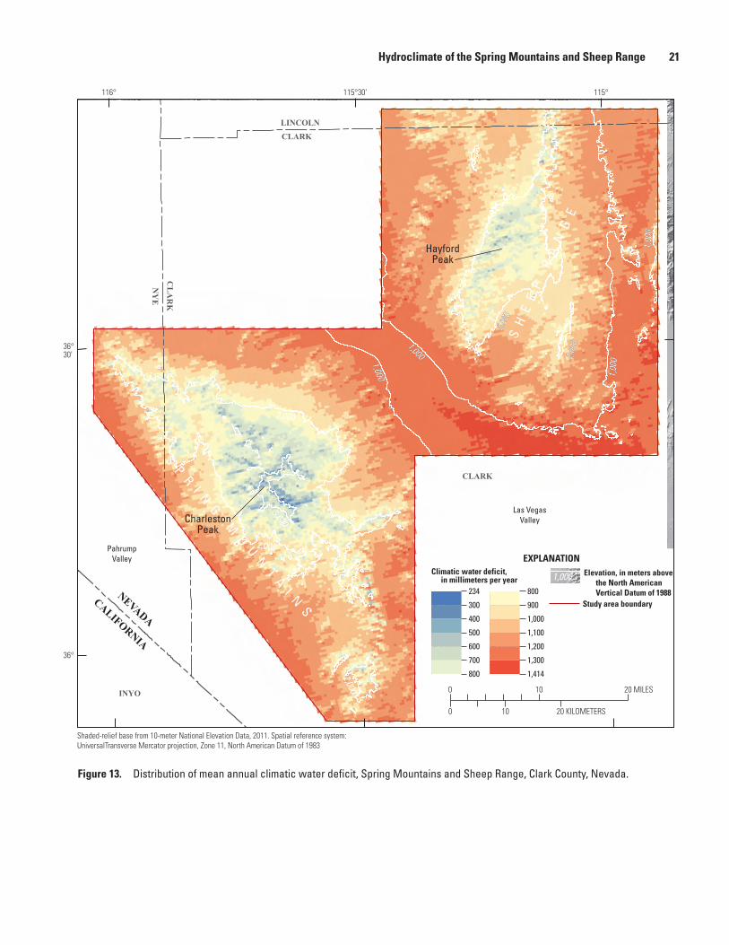
Hydroclimate of the Spring Mountains and Sheep Range 21
sac14-4204_fig 13
2,000
2,000
3,000
2,000
1,0001,000
1,00
01,
000
2,000
2,000
2,00
02,
000
1,0001,000
1,00
01,
000
NEVADA
CALIFORNIA
INYO
PahrumpValley
CharlestonPeak
HayfordPeak
LINCOLN
NY
E
CLARK
CL
AR
K
0 10 20 MILES
0 10 20 KILOMETERS
Study area boundary
1,000
EXPLANATIONClimatic water deficit,
in millimeters per year234
300
400
500
600
700
800
800
900
1,000
1,100
1,200
1,300
1,414
Elevation, in meters above the North American Vertical Datum of 1988
36°30'
36°
115°115°30'116°
Shaded-relief base from 10-meter National Elevation Data, 2011. Spatial reference system: UniversalTransverse Mercator projection, Zone 11, North American Datum of 1983
Las VegasValley
CLARK
SH
EE
P
RA
NG
ES
PR
I NG
MO
UN
TA
I NS
Figure 13. Distribution of mean annual climatic water deficit, Spring Mountains and Sheep Range, Clark County, Nevada.

22 Hydroclimate of the Spring Mountains and Sheep Range, Clark County, Nevada
Climate Zones and Aridity Index
Climate aridity provides information on the moistness or dryness of a region. Whether a climate is moist or dry cannot be determined by knowing precipitation alone—PET also must be known (Thornthwaite, 1948). Aridity can be computed as a function of precipitation and PET. Many numerical indices have been proposed to quantify the degree of dryness of a climate at a given location in an attempt to help delineate climate zones (Maliva and Missimer, 2012). The United Nations Educational and Scientific Organization (1979) proposed a classification of climate zones based on an aridity index, where the index is computed by dividing precipitation by PET. Climate zones for the current study are classified according to this conceptually simple and widely used classification system:
Hyper-arid = Aridity index < 0.03Arid = 0.03 < Aridity index < 0.20Semi-arid = 0.20 < Aridity index < 0.50Sub-humid = 0.50 < Aridity index < 0.75Humid = Aridity index > 0.75
The spatial distribution of climate zones throughout the study area is shown in figure 14. Arid regions have low precipitation and high PET rates, and therefore, low aridity index values. The low elevations in the study area are within the arid climate zone. The semi-arid climate zone generally begins in the blackbrush ecosystem at a mean elevation of about 1,560 m. The sub-humid zone is absent from the Sheep Range and begins in the mixed conifer ecosystem of the Spring Mountains at a mean elevation of about 2,660 m. The humid zone occurs primarily in small pockets on north- and northeast-facing slopes in the upper elevations of the Spring
Mountains where the topographic shading is greatest. Mean aridity index values for the four primary ecosystems in each mountain range are given in table 4. Computed aridity index data are included in the geospatial database (appendix A).
Water Balance Estimates
The water balance is a robust concept which can be applied at various spatial and temporal scales. A basin-scale water balance at the mean annual timescale has important implications because annual runoff and recharge to regional aquifers often determine the quantity of water available for human consumption. A water balance at the intra-annual scale provides the analytical framework for examining the spatial and temporal characteristics of wetting and drying periods (Shelton, 2009).
The water balance as presented in this study is an assessment of relations between moisture supply and demand at the seasonal site scale and mean-annual ecosystem scales. Precipitation provides the moisture supply, and the moisture demand is represented by AET. Recharge at the mean-annual ecosystem scale is expressed as the residual of precipitation depleted by AET. This simplification of the water balance is based on the assumption that the volume of runoff in the study area is minor in relation to recharge, and soil moisture levels remain approximately the same when averaged for a decade or more (Shelton, 2009). The seasonal site-scale water balance describes the changing seasonal relation between precipitation and AET where energy and moisture maxima contrast.
The seasonal water balance is explored by examining the relation between precipitation and AET from the Lee Canyon SNOTEL and EC stations using mean monthly data acquired from July 2008 through June 2010 (fig, 2).
Table 4. Mean annual ecosystem water budgets and hydroclimate data, Spring Mountains and Sheep Range, Clark County, Nevada.
[Mean values in millimeters unless otherwise noted. Abbreviations: AET, actual evapotranspiration; PET, potential evapotranspiration; CWD, climatic water deficit. Recharge: computed as precipitation minus AET. CWD: computed as PET minus AET. Aridity index: computed as precipitation divided by PET. Recharge efficiency: computed as recharge divided by precipitation]
Mountain range EcosystemElevation (meters)
Precipi- tation
AET Recharge PET CWDAridity index, dimensionless
Recharge efficiency,
dimensionless
Spring Mountains Blackbrush 1,517 277 267 10 1,347 1,080 0.21 0.03Pinyon-juniper 2,062 411 381 30 1,249 868 0.33 0.07Mixed conifer 2,533 510 427 83 1,133 706 0.45 0.16Bristlecone pine 3,012 574 422 152 1,075 653 0.53 0.27
Sheep Range Blackbrush 1,549 225 225 0 1,286 1,061 0.17 0.00Pinyon-juniper 2,107 312 303 9 1,180 877 0.26 0.03Mixed conifer 2,553 362 326 37 1,117 791 0.32 0.10Bristlecone pine 2,842 370 313 57 1,141 828 0.32 0.15

Hydroclimate of the Spring Mountains and Sheep Range 23
sac14-4204_fig 14
2,000
2,000
3,000
2,000
1,0001,000
1,00
01,
000
2,000
2,000
2,000
2,000
1,0001,000
1,00
01,
000
NEVADACALIFORNIA
INYO
PahrumpValley
Las VegasValley
HayfordPeak
CLARK
CharlestonPeak
LINCOLN
NY
E
CLARK
CL
AR
K
Scale 98%
SP
RI N
G M
OU
NT
AI N
S
SH
EE
P
RA
NG
EEXPLANATION
0 10 20 MILES
0 10 20 KILOMETERS
Aridity index and climatezones
0.08
0.20
0.50
0.75
1.03
Arid
Semi-arid
Sub-humid
Humid
Study area boundary
Elevation, in meters above the North American Vertical Datum of 1988
1,000
36°30'
36°
115°115°30'116°
Shaded-relief base from 10-meter National Elevation Data, 2011. Spatial reference system: UniversalTransverse Mercator projection, Zone 11, North American Datum of 1983
Figure 14. Distribution of mean annual (1971–2007) aridity index and climate zones, Spring Mountains and Sheep Range, Clark County, Nevada.

24 Hydroclimate of the Spring Mountains and Sheep Range, Clark County, Nevada
About 65 percent of annual precipitation fell during the cool season primarily as snow (fig. 15A). Generally, snow accumulated at the surface with each passing storm because the snowfall rate exceeded the combined rates of snowmelt and evaporation (sublimation). As a result, the mean monthly snow depth increased from 0 mm in October to 320 mm in March. From March to June the snow depth decreased to 0 mm as the available energy increased resulting in warming air temperatures, and snowmelt and sublimation rates that exceeded the decreasing precipitation rate. However, precipitation was considerable during July and August owing to summer convective storms. Mean annual precipitation for the period was 709 mm.
The mean monthly volumetric soil water contents (SWC) measured at the SNOTEL site for 0.2, 0.5, and 1 m depths below land surface are shown in figure 15B. As meltwater infiltrated the soil, a portion of it was stored in soil pores, raising the SWC. As the soil became wetter, its ability to conduct moisture increased until water was transmitted downward (percolation) as fast as the snowmelt infiltrated. Once this condition was reached, the SWC of the
surface became constant and a wave of moisture percolated downward, wetting successively deeper layers to a moisture content at which their hydraulic conductivity is equal to the infiltration rate (Dunne and Leopold, 1978). SWC increased at a relatively constant rate at each depth through May as meltwater percolated to 1 m. As the air temperature increased through spring, so did the biological activity. In addition to water being lost from the site through infiltration and percolation processes, water vapor also was lost to the atmosphere as carbon dioxide diffused through ponderosa pine leaf stomata for photosynthesis. This transpired water was replaced by soil water moving, from high to low potential from root system through the xylem to the leaves, in response to transpiration demand. Ponderosa pine roots can range in depth from less than 1 to more than 2 m (Burns and Honkala, 1990). The trend in soil moisture decreased from May through December because the combined rates of ponderosa pine transpiration and percolation deeper than 1 m exceeded the combined rates of residual snowmelt percolation and percolation of new and mostly liquid precipitation (rain) into the 0.2–1-m depth range.
sac14-4204_fig15
0
50
100
150
200
250
300
350
Jan. Feb. Mar. Apr. May June July Aug. Sep. Oct. Nov. Dec. Jan. Feb. Mar. Apr. May June July Aug. Sep. Oct. Nov. Dec.
Prec
ipita
tion
and
snow
dep
th, i
n m
illim
eter
s
Snow depth
0
10
20
30
40
50
60
0
5
10
15
20
25
30
AET,
in m
illim
eter
s
Volu
met
ric s
oil w
ater
con
tent
, in
perc
ent
SWC -0.2 m
SWC -0.5 m
AET
EXPLANATIONEXPLANATION
A B
Precipitation
SWC -1 m
Figure 15. Intra-annual patterns of mean monthly (A) precipitation and snow depth measured at the Lee Canyon Snowpack Telemetry (SNOTEL) station, and (B) volumetric soil water content (SWC) and actual evapotranspiration (AET) measured at Lee Canyon SNOTEL and eddy-covariance (EC) stations, July 2008 through June 2010, Spring Mountains, Clark County, Nevada. (SWC measured at depths below land surface, in meters [m].)

Hydroclimate of the Spring Mountains and Sheep Range 25
Figure 15B also shows mean monthly AET measured at the sub-canopy EC station. AET generally increased from January through May as increasing available energy during this period converted water from a solid (snow) to liquid (snowmelt) and vapor phases. The process that converts snow directly to vapor is sublimation. Sublimation accounted for approximately 100 percent of AET from January through May because the site was approximately 100 percent covered in snow (fig. 15A). In June, AET decreased as the snow-free, near-surface soil moisture decreased as indicated by the SWC at 0.2 m depth. AET increased during July and August in response to summer convective storms, and some of this precipitation increased or maintained the SWC downward to 1 m. AET and soil moisture generally decreased through October then responded to storm events in November and December at the shallow depths. It should be reiterated that EC measurements primarily reflected sublimation and ground evaporation processes because the EC sensors were positioned below the ponderosa pine forest canopy. The mean annual AET measured at the EC station was 283 mm.
A water balance for Lee Canyon can be estimated on the basis of site-specific measurements and previously published values as follows. The primary objective of any water balance analysis is to determine the effect of precipitation. Mean annual precipitation for the 2-year measurement period (July 2008–June 2010) was 709 mm. Of this amount, 283 mm (40 percent) was lost to the atmosphere to sublimation and sub-canopy evaporation processes. Data are not sufficient to divide the remaining precipitation between the amount used for transpiration and the amount that percolated past root zones (recharge). Assuming the estimate reported by Ryan and others (2000) is reasonably applicable to the current study area, 117 mm (17 percent of precipitation) was transpired by the ponderosa pine forest; therefore, the remaining amount of 309 mm (43 percent) became recharge. Recharge may be either local or regional. Local recharge is deeply percolating water that is captured by local perched aquifers (within the Spring Mountains) and discharged to local springs. Regional recharge is deeply percolating water that travels through the highly-fractured Paleozoic carbonate bedrock and discharges to adjacent or downgradient groundwater basins. For this site-scale water balance, it is not known what portion of deeply percolating subsurface water is captured for regional as opposed to local recharge processes; however, a large percentage of this water potentially is regional recharge because estimates of local spring discharge in Lee Canyon are small (Plume, 1984). The seasonal water balance pattern presented in this section based on data from the Lee Canyon SNOTEL and EC stations should be reasonably representative of the mixed conifer ecosystem in the Spring Mountains because the intra-annual energy and moisture minima and maxima should be similar, allowing for local deviations based primarily on varying topography. It should be noted that precipitation during the 2-year period of this analysis (709 mm) is about 30 percent greater than the 1971–2007 PRISM mean (545 mm).
A water balance is computed at the mean annual timescale from PRISM precipitation and VegET AET datasets for each of the four primary ecosystems (table 4). Precipitation and AET are substantially greater in the Spring Mountains than in the Sheep Range. Recharge in the Spring Mountains is greater than in the Sheep Range because the difference between precipitation and AET is greater (table 4, fig. 12A). For example, mean annual precipitation in the bristlecone pine ecosystem of the Spring Mountains is 55 percent greater than in the Sheep Range, AET is 34 percent greater, and the resulting recharge estimate is 269 percent greater in the Spring Mountains than in the Sheep Range.
Recharge can be expressed in terms of the percentage of precipitation that becomes recharge, or the recharge efficiency. For the bristlecone pine ecosystem, 27 percent of precipitation becomes recharge in the Spring Mountains compared to only 15 percent in the Sheep Range. For the mixed conifer ecosystem, 16 percent of precipitation becomes recharge in the Spring Mountains compared to 10 percent in the Sheep Range (table 4).
Recharge efficiencies also are computed as a function of elevation at 10-m increments in each range (fig. 16). The recharge efficiency is greater at all elevations in the Spring Mountains than in the Sheep Range. Mean annual recharge estimates are assumed to be regional because the relatively small amount of local recharge is accounted for indirectly as AET through NDVI variability in the VegET model. Recharge computed for the study area is within the range of previous estimates (see section “Evapotranspiration Estimates”). Computed recharge data are included in the geospatial database (appendix A).
sac14-4204_fig16
y = 7E-06x2
2 - 0.0174x + 11.919
R = 0.9692
y = 5E-06x2
2 - 0.0117x + 7.3064
R = 0.9343 0
10
20
30
40
50
60
1,000 2,000 3,000 4,000
Rech
arge
, as
perc
ent o
f pre
cipi
tatio
n
Elevation, in meters
Figure 16. Recharge efficiency as a function of elevation, Spring Mountains and Sheep Range, Clark County, Nevada.

26 Hydroclimate of the Spring Mountains and Sheep Range, Clark County, Nevada
SummaryThe U.S. Forest Service is conducting a study to better
understand and delineate ecological zones in the Spring Mountains and Sheep Range of southern Nevada. Because hydroclimate data are sparse in this area of high topographic-climatic variability, land management agencies lack sufficient information to understand the relation between hydroclimatic variables and the distribution and productivity of ecological zones, or how ecological zones may be affected by climate change. As part of this overall study, the U.S. Geological Survey (USGS) is characterizing the local hydroclimate with an emphasis on the magnitude, timing, and distribution of precipitation and evapotranspiration. The remote-sensing and model-based methodology of this research stems from the challenges posed by limited access and sparse data in this mountainous environment.
Spatially and temporally explicit estimates of precipitation, potential evapotranspiration (PET), and actual evapotranspiration (AET) are compiled, developed, and used to characterize the local hydroclimate. Mean annual precipitation estimates (1971–2007) are based on monthly Parameter-elevation Regressions on Independent Slopes Model (PRISM) 800-meter (m) gridded data. Mean annual PET estimates (1971–2007) are developed from monthly Basin Characterization Model (BCM) 270-m gridded data. Mean annual AET is estimated using two remote-sensing models. The first model—Operational Simplified Surface Energy Balance (SSEBop)—uses an energy balance approach. The second model—Vegetation Evapotranspiration (VegET)—uses a water balance approach. Both models rely on Moderate Resolution Imaging Spectroradiometer (MODIS) data.
Model results are validated with limited ground measurements. Compared to four high elevation precipitation gages with more than 20 years of record, PRISM underestimates precipitation by 7–15 percent. Precipitation at 3,000-m elevation is 50 percent greater in the Spring Mountains than in the Sheep Range. The lesser amount of precipitation in the Sheep Range is attributed to partial moisture depletion by the Spring Mountains of eastward-moving cool-season (October–April) storms, which accounts for 66–76 percent of annual precipitation. PET estimates by the BCM range from about 700 millimeter (mm) in the upper elevations (> 2,800 m) of the Spring Mountains to 1,600 mm in the lower elevations. The VegET model simulated AET more accurately than the SSEBop model at the annual timescale. Mean annual VegET AET estimates (2001–11) range from about 100 to 600 mm. A simple water budget validates the magnitude of mean annual VegET AET where regional recharge is estimated by subtracting VegET AET from PRISM precipitation. The budget assumes that (1) runoff in the study area is minor, (2) PRISM-estimated precipitation is reasonably accurate, and (3) changes in soil moisture storage are negligible on a mean annual basis. The resulting recharge estimate to the underlying groundwater flow system is within the range of recharge estimated by previous studies.
Hydroclimatic variables compiled and calculated for this study are correlated to ecosystem distributions and to each other for exploring the spatial and temporal variability and relations between variables, elevation, and ecosystem distribution. Aridity-index-based climate zones and climatic water deficit datasets are developed from precipitation and evapotranspiration datasets. Climate zones range from arid, in the lower elevations of the study area, to humid, in small pockets adjacent to north- and northeast-facing slopes in the upper elevations of the Spring Mountains. Correlative analyses between hydroclimatic variables and mean ecosystem elevations indicate that the climatic water deficit is the best predictor of ecosystem distribution. Computed water balances indicate substantially more recharge is generated in the Spring Mountains than in the Sheep Range. A geospatial database containing compiled and developed hydroclimatic data and other pertinent information accompanies this report.
References Cited
Allen, R.G., Pereira, L.S., Raes, D., and Smith, M., 1998, Crop evapotranspiration—Guidelines for computing crop water requirements: Rome, FAO Irrigation and Drainage Paper 56, Food and Agriculture Organization of the United Nations, 300 p.
Allen, R.G., Tasumi, M., Morse, A.T., Trezza, R., Kramber, W., Lorite, I., and Robison, C.W., 2007, Satellite-based energy balance for mapping evapotranspiration with internalized calibration (METRIC)—Applications: ASCE Journal of Irrigation and Drainage Engineering, v. 133, p. 395–406.
Bastiaanssen, W.G.M., Menenti, M., Feddes, R.A., and Holtslag, A.A.M., 1998, A remote sensing surface energy balance algorithm for land (SEBAL)—1. Formulation: Journal of Hydrology, v. 212–213, p. 198–212.
Belcher, W.R., and Sweetkind, D.S., eds., 2010, Death Valley regional groundwater flow system, Nevada and California—Hydrogeologic framework and transient groundwater flow model: U.S. Geological Survey Professional Paper 1711, 398 p.
Burns, R.B., and Honkala, B.H., 1990, Silvics of North America—1. Conifers: Washington D.C., U.S. Department of Agriculture, U.S. Forest Service, Agriculture handbook 654, v. 2, 877 p.
Choudhury, B.J., Ahmed, N.U., Idaho, S.B., Reginato, R.J., and Daughtry, C.S.T., 1994, Relations between evaporation coefficients and vegetation indices: studies by model simulation: Remote Sensing of Environment, v. 50, 1–17.

References Cited 27
Clark County, 2000, Final Clark County multiple species habitat conservation plan and environmental impact statement for issuance of a permit to allow incidental take of 79 species in Clark County, Nevada, September 2000: Las Vegas, Nevada, Prepared by RECON for Clark County Department of Comprehensive Planning, [variously paged].
Daly, C., Halbleib, M., Smith, J.I., Gibson, W.P., Doggett, M.K., Taylor, G.H., Curtis, J., and Pasteris, P.P., 2008, Physiographically sensitive mapping of climatological temperature and precipitation across the conterminous United States: International Journal of Climatology, v. 28, no. 15, p. 2,031–2,064.
Dettinger, M.D., 1989, Reconnaissance estimates of natural recharge to desert basins in Nevada, U.S.A., by using chloride balance calculations: Journal of Hydrology, v. 106, p. 55–78.
Dunne, T., and Leopold, L.B., 1978, Water in environmental planning: New York, W.H. Freeman and Company, 818 p.
Fenelon, J.M., and Moreo, M.T., 2002, Trend analysis of ground-water levels and spring discharge in the Yucca Mountain region, 1960–2000: U.S. Geological Survey Water-Resources Investigations Report 02-4178, 97 p., http://pubs.usgs.gov/wri/wrir024178/.
Flint, A.L., and Childs, S.W., 1987, Calculation of solar radiation in mountainous terrain: Agricultural and Forest Meteorology, v. 40, p. 233–249.
Flint, A.L. and Childs, S.W., 1991, Modification of the Priestley-Taylor equation to estimate evapotranspiration for soil water limited conditions: Agricultural and Forest Meteorology, v. 56, p. 247–260.
Flint, L.E., and Flint, A.L., 2007a, Regional analysis of ground-water recharge, in Stonestrom, D.A., Constantz, J., Ferré, T.P.A., and Leake, S.A., eds., Ground-water recharge in the arid and semiarid southwestern United States: U.S. Geological Survey Professional Paper 1703, p. 29–59, http://pubs.usgs.gov/pp/pp1703/b/.
Flint, L.E., and Flint, A.L., 2007b, Estimation of hourly stream temperatures in unmeasured tributaries to the lower Klamath River, California: Journal of Environmental Quality, v. 37, p. 57–68.
Flint, L.E., and Flint, A.L., 2012, Downscaling future climate scenarios to fine scales for hydrologic and ecologic modeling and analysis: Ecological Processes, v. 1, p. 1–15.
Flint, L.E., Flint, A.L., Stolp, B.J., and Danskin, W.R., 2012, A basin-scale approach for assessing water resources in a semiarid environment—San Diego region, California and Mexico: Hydrology and Earth System Sciences, v. 16, p. 3,817–3,833.
Harrill, J.R., 1976, Pumping and ground-water storage depletion in Las Vegas Valley, Nevada, 1955–74: Nevada Department of Conservation and Natural Resources, Division of Water Resources Bulletin No. 44, 70 p.
Harrill, J.R., 1986, Ground-water storage depletion on Pahrump Valley, Nevada-California, 1962–75: U.S. Geological Survey Water-Supply Paper 2279, 116 p.
Harrill, J.R., and Prudic, D.E., 1998, Aquifer systems in the Great Basin region of Nevada, Utah, and adjacent states—summary report: U.S. Geological Survey Professional Paper 1409-A, 66 p.
Hess, R.H., and Johnson, G.L., 1996, County digital geological maps of Nevada: Nevada Bureau of Mines and Geology Open-File Report 97-1.
Heaton, J.S., Miao, X., Von Seckendorff Hoff, K., Charlet, D., Cashman, P., Trexler, J., Grimmer, A., and Patil, R., 2011, Ecosystem indicators final report 2005-UNR-578, report to Clark County MSHCP: University of Nevada Reno, 36 p.
Houghton, J.G., Sakamato, C.M., and Gifford, R.O., 1975, Nevada’s weather and climate: Nevada Bureau of Mines and Geology Special Publication 2, 78 p.
Larsen, L.W., and Peck, E.L., 1974, Accuracy of precipitation measurements for hydrologic modeling: Water Resources Research, v. 10, no. 4, p. 857–863.
Maliva, R., and Missimer, T., 2012, Arid lands water evaluation and management: Springer-Verlag Berlin, 1,076 p.
Malmberg, G.T., 1965, Available water supply of the Las Vegas ground-water basin, Nevada: U.S. Geological Survey Water-Supply Paper 1780, 116 p., 13 pls.
Malmberg, G.T., 1967, Hydrology of the valley-fill and carbonate-rock reservoirs, Pahrump Valley, Nevada-California: U.S. Geological Survey Water-Supply Paper 1832, 47 p.
Maxey, G.B., and Jameson, C.H., 1948, Geology and water resources of Las Vegas, Pahrump, and Indian Springs Valleys, Clark and Nye Counties, Nevada: Nevada State Engineer Water Resources Bulletin 5, 121 p.
Moreo, M.T., Laczniak, R.J., and Stannard, D.I., 2007, Evapotranspiration rate measurements of vegetation typical of ground-water discharge areas in the Basin and Range carbonate-rock aquifer system, White Pine County, Nevada, and adjacent areas in Nevada and Utah, September 2005–August 2006: U.S. Geological Survey Scientific Investigations Report 2007-5078, 36 p., http://pubs.er.usgs.gov/publication/sir20075078.

28 Hydroclimate of the Spring Mountains and Sheep Range, Clark County, Nevada
Moreo, M.T., and Swancar, A., 2013, Evaporation from Lake Mead, Nevada and Arizona, March 2010 through February 2012: U.S. Geological Survey Scientific Investigations Report 2013–5229, 40 p., http://dx.doi.org/10.3133/sir20135229.
Page, W.R., Lundstrom, S.C., Harris, A.G., Langenheim, V.E., Workman, J.B., Mahan, S.A., Paces, J.B., Dixon, G.L., Rowley, P.D., Burchfiel, B.C., Bell, J.W., and Smith, E.I., 2005, Geologic and Geophysical maps of the Las Vegas 30’ × 60’ quadrangle, Clark and Nye Counties, Nevada, and Inyo County, California: U.S. Geological Survey Scientific Investigations Map 2814, http://pubs.usgs.gov/sim/2005/2814/.
Plume, R.W., 1984, Ground-water resources of Kyle and Lee Canyons, Spring Mountains, Clark County, Nevada: U.S. Geological Survey Open-File Report, 47 p., http://pubs.er.usgs.gov/publication/ofr84438.
Priestley, C.H.B., and Taylor, R.J., 1972, On the assessment of surface heat flux and evaporation using large-scale parameters: Monthly Weather Review, v. 100, p. 81–92.
Prior-Magee, J.S., Boykin, K.G., Bradford, D.F., Kepner, W.G., Lowry, J.H., Schrupp, D.L., Thomas, K.A., and Thompson, B.C., eds, 2007, Ecoregional gap analysis of the southwestern United States: Moscow, Idaho, The Southwest Regional Gap Analysis Project Final Report, U.S. Geological Survey gap analysis program, 441 p.
PRISM Climate Group, 2008, PRISM climate data created July, 2008: Corvallis, Oregon, Oregon State University, http://prism.oregonstate.edu.
Quiring, R.F., 1965, Annual precipitation amount as a function of elevation in Nevada south of 38 ½ degrees latitude, Las Vegas, Nevada: U.S. Weather Bureau Research Station, 14 p.
Ralph, F.M., Neiman, P.J., Kingsmill, D.E., Persson, P., White, A.B., Strem, E.B., Andrews, E.D., and Antweiler, R.C., 2003, The impact of a prominent rain shadow on flooding in California’s Santa Cruz Mountains—A CALJET case study and sensitivity to the ENSO cycle: Journal of Hydrometeorology, v. 4, p. 1,243–1,264.
Randall, J.M., Parker, S.S., Moore, J., Cohen, B., Crane, L., Christian, B., Cameron, D., MacKenzie, J., Klausmeyer, K., and Morrison, S., 2010, Mojave Desert ecoregional assessment: San Francisco, California, The Nature Conservancy, unpublished report, September 2010, version 1.1, 106 p., http://conserveonline.org/workspaces/mojave/documents/mojave-desert-ecoregional-2010/@@view.html.
Ryan, M.G., Bond, B.J., Law, B.E., and others, 2000, Transpiration and whole-tree conductance in ponderosa pine trees of different heights: Oecologia, v. 124, p. 553–560.
San Juan, C.A., Belcher, W.R., Laczniak, R.J., and Putnam, H.M., 2000, Chapter C—Hydrologic components for model development, in Belcher, W.R., and Sweetkind, D.S., eds., 2010, Death Valley regional groundwater flow system, Nevada and California—Hydrogeologic framework and transient groundwater flow model: U.S. Geological Survey Professional Paper 1711, 398 p.
Senay, G.B., 2008, Modeling landscape evapotranspiration by integrating land surface phenology and a water balance algorithm: Algorithms, v. 1, p. 52–68.
Senay, G.B., Bohms, S., Singh R., Gowda, P., Velpuri, N.M., Alemu, H., and Verdin, J.P., 2013, Operational evapotranspiration modeling using remote sensing and weather datasets—A new parameterization for the SSEB approach: Journal of the American Water Resources Association, v. 49, no. 3, p. 577–591.
Senay, G.B., and Verdin, J.P., 2003, Characterization of yield reduction in Ethiopia using a GIS-based crop water balance model: Canadian Journal of Remote Sensing, v. 29, p. 687–692.
Shelton, M.L., 2009, Hydroclimatology—Perspectives and applications: Cambridge University Press, New York, 426 p.
Simon, S.A., Collins, T.K., Kauffman, G.L., McNab, W.H., and Ulrey, C.J., 2005, Ecological zones in the southern Appalachians—First approximation: U.S. Forest Service Research Paper SRS-41, 41 p.
Soil Survey Staff, 2011, Web Soil Survey: Natural Resources Conservation Service, United States Department of Agriculture—, accessed April 24, 2012, at http://websoilsurvey.nrcs.usda.gov/.
Soil Survey Staff, 2012, Soil Survey Geographic (SSURGO) Database for Survey Areas 608, 755, 757, 785, 788, Nevada: Natural Resources Conservation Service, U.S. Department of Agriculture, accessed May 25, 2012, at http://websoilsurvey.sc.egov.usda.gov/App/HomePage.htm.
Stephenson, N.L., 1998, Actual evapotranspiration and deficit—Biologically meaningful correlates of vegetation distribution across spatial scales: Journal of Biogeography, v. 25, p. 855–870.
Stonestrom, D.A., Constantz, J., Ferre, Ty P.A., and Leake, S.A., eds., 2007, Ground-water recharge in the arid and semiarid southwestern United States: U.S. Geological Survey Professional Paper 1703, 414 p., http://pubs.usgs.gov/pp/pp1703/.

References Cited 29
Tasumi, M., and Allen, R.G., 2007, Satellite-based ET mapping to assess variation in ET with timing of crop development: Agricultural Water Management, v. 88, p. 54–62.
Thomas, J.M., Welch, A.H., and Dettinger, M.D, 1996, Geochemistry and isotope hydrology of representative aquifers in the Great Basin region of Nevada, Utah, and adjacent states: U.S. Geological Survey Professional Paper 1409-C, 100 p., http://pubs.er.usgs.gov/publication/pp1409C.
Thorne, J.H., Boynton, R., Flint, L.E., Flint, A. L., and Thuy, N.L., 2012, Development and application of downscaled hydroclimatic predictor variables for use in climate vulnerability and assessment studies: California Energy Commission, no. CEC-500-2012-010, 84 p.
Thornthwaite, C.W., 1948, An approach toward a rational classification of climate: Geographical Review, v. 38, no. 1, p. 55–94.
The Nature Conservancy, 2001, Mojave Desert Ecoregional assessment: The Nature Conservancy of California, v 1.1, 210 p., http://www.azconservation.org.
United Nations Educational and Scientific Organization, 1979, Map of world distribution of arid regions: Paris, United Nations Educational and Scientific Organization, Map at scale 1:25,000,000 with explanatory note MAB technical notes 7, 54 p.
U.S. Fish and Wildlife Service, 2013, Ash Meadows National Wildlife Refuge, Nevada—Wildlife and Habitat: U.S. Fish and Wildlife Service Web page, accessed March 4, 2014, at http://www.fws.gov/refuge/Ash_Meadows/wildlife_and_habitat/index.html.
U.S. Geological Survey, 1999, National Elevation Dataset: U.S. Geological Survey Fact Sheet 148-99, 2 p.
Walker, G.E., and Eakin, T.E., 1963, Geology and ground water of Amargosa Desert, Nevada–California: Nevada Department of Conservation and Natural Resources, Ground-Water Resources—Reconnaissance Report 14, 44 p.
Western Region Climate Center, 2014, precipitation data for Las Vegas WSO Airport, Nevada (264436): Western Regional Climate Center accessed June 18, 2014, at http://www.wrcc.dri.edu/cgi-bin/cliMAIN.pl?nv4436.


Appendixes 31
Appendix A. Geospatial Database, Spring Mountains and Sheep Range, Clark County, Nevada
An Environmental Systems Research Institute (ESRI) ArcGIS 10.1 file geodatabase was compiled to support any future efforts to characterize ecological zones. The file geodatabase contains a vector point feature class consisting of 81,481 points arranged in a 270-m grid that covers the study area (fig. 1). ArcGIS tools were used to extract data from raster and vector geospatial datasets and relate those data to the points as attributes. Attributes include the hydroclimatic variables discussed in this report (table A1) and other ancillary data. Hydroclimate and ancillary datasets are described in the metadata for the file geodatabase. The appendix A file geodatabase is available for download at http://pubs.water.usgs.gov/sir/2014/5142/.
Table A1. Hydroclimate attributes in geodatabase, Spring Mountains and Sheep Range, Clark County, Nevada.
[Abbreviations: PRISM, Parameter-elevation Regressions on Independent Slopes Model; mm, millimeter; °C, degrees Celsius; BCM, Basin Characterization Model; VegET, Vegetation Evapotranspiration; PET, potential evapotranspiration; AET, actual evapotranspiration; CWD, climatic water deficit; N/A, not applicable]
Attribute identifier
Hydroclimatic variable
ModelPeriod of record
(water year)
Computed period of
record statisticUnit Reference Remarks
PPT_PRISM_mm Precipitation PRISM 1971–2007 Mean mm Daly and others, 2008
N/A
TM_PRISM_C Minimum temperature
PRISM 1971–2007 Mean °C Daly and others, 2008
N/A
TX_PRISM_C Maximum temperature
PRISM 1971–2007 Mean °C Daly and others, 2008
N/A
PET_BCM_mm PET BCM 1971–2007 Mean mm Flint and Flint, 2007a
N/A
AET_VegET_mm AET VegET 2001–2011 Mean mm Current study N/ACWD_cmp_mm CWD N/A N/A N/A mm Current study Computed as PET minus
AETRCH_cmp_mm Recharge N/A N/A N/A mm Current study Computed as precipitation
minus AET; values less than 0 set to 0
AI_cmp Aridity index N/A N/A N/A Dimension- less
Current study Computed as precipitation divided by PET

32 Hydroclimate of the Spring Mountains and Sheep Range, Clark County, Nevada
Appendix B. Evapotranspiration Data, Spring Mountains and Sheep Range, Clark County, Nevada
A spreadsheet of pertinent evapotranspiration data in Microsoft® Excel 2010 format is available at http://pubs.usgs.gov/sir/2014/5142/. Column headers are described within the spreadsheet; selected daily data are presented in native units. Eddy covariance latent- and sensible-heat flux data are not corrected for energy imbalances at daily or sub-daily time steps. Appendix B daily data are available for download at http://pubs.water.usgs.gov/sir/2014/5142/. Sub-daily (20- and 30-minute) data are available for download at http://nevada.usgs.gov/water/et/index.htm.

Appendixes 33
Appendix C. Evaluation of Over-Estimation of Actual Evapotranspiration by the Operational Simplified Surface Energy Balance Model in High-Elevation Areas, Spring Mountains and Sheep Range, Clark County, Nevada
cooler in 2010 than 2005 for Tmax. If we assume, the MODIS sensor is stable for LST, then it raises the question whether Tmax was unrealistically high in 2005.
A plot of yearly lapse rate from 2001 through 2012 using Daymet and LST data shows that the lapse rate from Ta showed erratic behavior and, on average, lower estimates for the 2001–06 as compared to the period since 2007 (fig. C3). Conversely, the lapse rate from LST also showed erratic patterns, but was consistently higher than the Ta lapse rate throughout the 12-year period. The 12-year average lapse rate from Ta was -0.008 K/m and -0.01 K/m for LST. The stability and higher average lapse rate since 2007 suggests that Daymet may have obtained data from new stations that improved the estimation of Ta in higher elevation areas. Note that the average of 2001–07 PRISM data was used for this study. Thus, comparing this period with 2007–12 may indicate a potential bias, especially in the use of the earlier year dataset. Therefore, we investigated the lapse rate differences for the two periods (2001–06 versus 2007–12) using average temperature for both Ta and LST. The premise is that if the lapse rate of the LST remains relatively constant from period to period (knowing the possible fluctuation from year to year) but the lapse rate from Daymet changes, then it points to a change in data or modeling change for the Daymet dataset.
Figure C4 shows the lapse rate for Tmax and LST for the two periods. The Tmax lapse rate changed from -0.0074 K/m (2001–06) to -0.0084 K/m (2007–12), but lapse rate from LST remained about the same, -0.0099 to -0.01 K/m. These findings point to two important conclusions:
1. The lapse rate between LST and Tmax differs in the study area; thus, relations established at lower elevations that assume a similar lapse rate for both LST and Tmax will introduce error into the ETf calculation. Note that once elevation differences are accounted by using Tmax, which accounts for lapse rate, the SSEBop model assumes that differences in LST are a result of latent-heat flux. It is important to remember that LST already accounts for lapse rate because it is a direct observation and not modeled.
2. The lapse rate of Tmax changed for the two periods, lower in 2001–06 (-0.0074 K/m) and higher in 2007–12 (-0.0084 K/m) while the lapse rate of LST remained at -0.01 K/m, indicating a change in data input or algorithm for Tmax.
Simulated operational Simplified Surface Energy Balance (SSEBop) actual evapotranspiration (AET) was substantially greater than AET simulated with the Vegetation Evapotranspiration model over elevated areas, particularly greater than 2,000 m. The overestimation increased with elevation. Owing to a heavy reliance of the SSEBop approach on the air temperature (Ta) for the cold boundary condition, an investigation was conducted to evaluate whether Ta and land surface temperature (LST) were experiencing differential lapse rates. From the SSEBop formulation, the major assumption is that the Ta and LST decrease with elevation with a comparable lapse rate. However, a Ta lapse rate smaller than the LST will result in a higher Ta estimation with elevation which in turn leads to a higher estimation of the ET fraction (ETf) and AET.
The 2001–06 Parameter-elevation Regressions on Independent Slopes Model (PRISM) maximum air temperature (Tmax) dataset available at the time of the study was evaluated along with MODerate Resolution Imaging Spectroradiometer (MODIS) LST for the same period along cross-section A-A′ (fig. C1). A daily 1-km gridded Daymet model Tmax dataset from 2001–12 (http://daymet.ornl.gov/overview) also was evaluated. It is important to note that the SSEBop model was run using PRISM Tmax whereas Daymet Tmax is only used to show time-series analysis over a longer time frame. A comparison between PRISM and Daymet Tmax show a strong correspondence; therefore, the use of Daymet in place of PRISM data is not expected to change the conclusion of the analysis (fig. C2). For 2010, because there was no PRISM data (at the time of the study), the median of 2001–06 is plotted for relative comparison. Daymet and PRISM Tmax correspond well in 2005; however, both plot much higher than the LST for elevations above 2,500 m. Differences between Tmax and LST are spatially distributed over a broad area and may not be attributed to cold LST due to snow. A snow-cover map from MODIS shows negligible snow during the same period. In 2010, the 2001–06 average PRISM Tmax plots higher than the 2010 Daymet Tmax and close to or higher than the LST. The areal extent of the PRISM dataset was smaller than Daymet, thus PRISM shows a shorter profile.
Generally, the change in temperature with elevation was at a lower rate for Tmax than the LST (fig. C2). Furthermore, the change in temperature with elevation (lapse rate) appears to be different for 2005 and 2010 for Tmax but about the same for LST. At the peak, the LST is cooler in 2005 than 2010, but

34 Hydroclimate of the Spring Mountains and Sheep Range, Clark County, Nevada
sac14-4204_fig C1
"
A
A'
NEVADA
CALIFORNIA
0 30 KILOMETERS10 20
0 10 20 30 MILESBase U.S. Geological Survey mean 30 arc-seconds GMTED2010(Global Multi-resolution Terrain Elevation Data 2010)Horizontal datum WGS84/Vertical datum EGM96 geoidU.S. Census Bureau Tiger/Line 2010
116˚00’
36˚30’
36˚00’
115˚30’ 115˚00’
ARIZONA
UTAHNEVADA
CALIFORNIA
EXPLANATION
Elevation, in meters above the North American Vertical Datum of 1988
Study area
Profile A–A’
Lee CanyonStation
4,000
0
Figure C1. The A-A’ cross-section used for lapse-rate comparisons, Spring Mountains and Sheep Range, Clark County, Nevada.

Appendixes 35
sac14-4204_fig C2
Distance from point A, in kilometers (figure C1)Distance from point A, in kilometers (figure C1)
A B
250
260
270
280
290
300
310
320Te
mpe
ratu
re, i
n de
gree
s ke
lvin
0
500
1,000
1,500
2,000
2,500
3,000
3,500
4,000
Elev
atio
n, in
met
ers
Tmax (daymet)Tmax (PRISM)LSTElevation
EXPLANATION
0 10 20 30 40 50 60 70 80 90 100 0 10 20 30 40 50 60 70 80 90 100
Figure C2. Maximum air temperature (Tmax), land-surface temperature (LST), and elevation for a profile, average for May 9–15, during 2005 and 2010, Spring Mountains, Mountains and Sheep Range, Clark County, Nevada.
sac14-4204_fig C3
Elevation, in meters
0.005
0.007
0.009
0.011
0.013
0.015
2001 2002 2003 2004 2005 2006 2007 2008 2009 2010 2011 2012
Laps
e ra
te, i
n de
gree
s ke
lvin
per
met
er
EXPLANATIONTmax (daymet)LST
Figure C3. Yearly lapse rate for May 9–15 using Daymet maximum air temperature (Tmax) and land-surface temperature (LST) (8-day average) data from 2001 through 2012, Spring Mountains and Sheep Range, Clark County, Nevada.
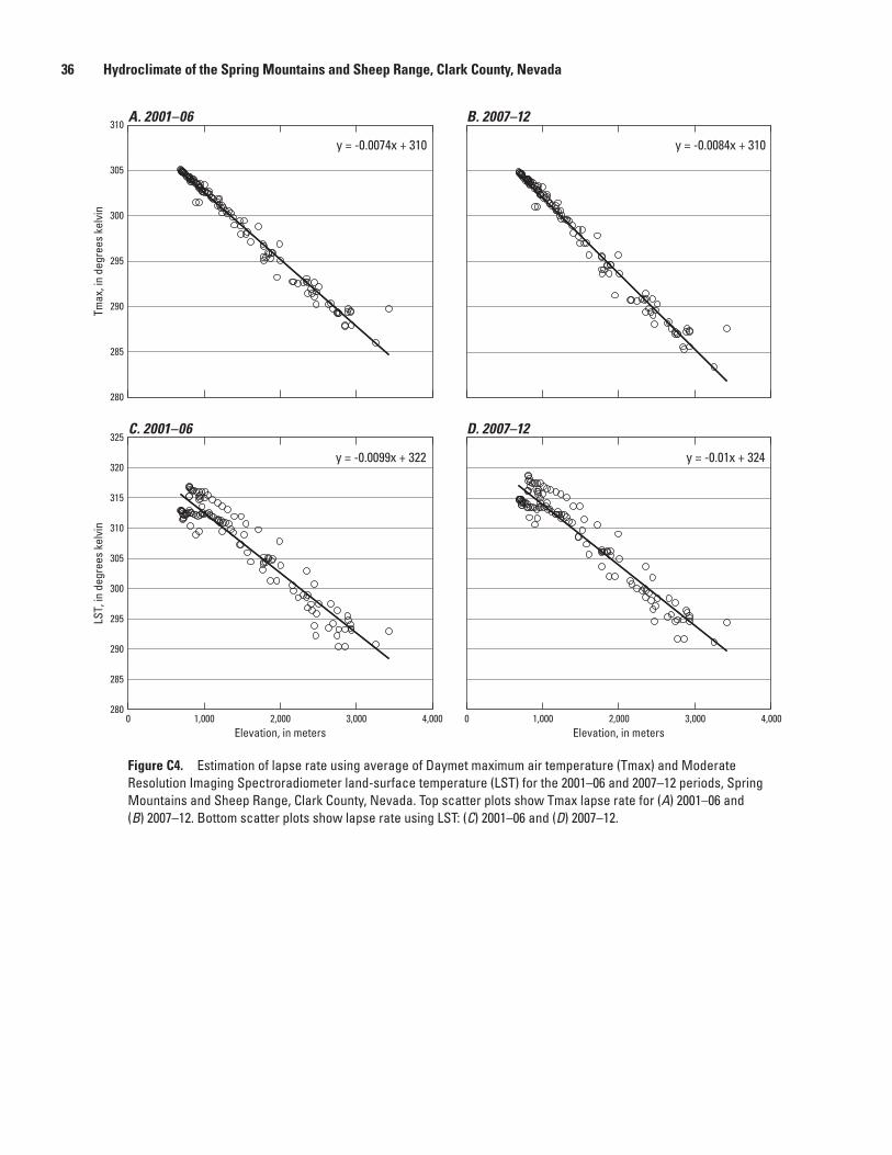
36 Hydroclimate of the Spring Mountains and Sheep Range, Clark County, Nevada
sac14-4204_fig C4
A. 2001–06 B. 2007–12
C. 2001–06 D. 2007–12
280
285
290
295
300
305
310
Tmax
, in
degr
ees
kelv
in
280
285
290
295
300
305
310
315
320
325
0 1,000 2,000 3,000 4,000
LST,
in d
egre
es k
elvi
n
0 1,000 2,000 3,000 4,000Elevation, in metersElevation, in meters
y = -0.0074x + 310
y = -0.0099x + 322
y = -0.0084x + 310
y = -0.01x + 324
Figure C4. Estimation of lapse rate using average of Daymet maximum air temperature (Tmax) and Moderate Resolution Imaging Spectroradiometer land-surface temperature (LST) for the 2001–06 and 2007–12 periods, Spring Mountains and Sheep Range, Clark County, Nevada. Top scatter plots show Tmax lapse rate for (A) 2001–06 and (B) 2007–12. Bottom scatter plots show lapse rate using LST: (C) 2001–06 and (D) 2007–12.

Appendixes 37
The relatively lower estimate of lapse rate for Tmax compared to LST results in a higher Tmax at higher elevations. This artificially elevates the cold boundary condition in the model. With elevated cold boundary conditions, observed LST from satellite will be plotted close to the cold boundary conditions, which increases the ETf, and thus the modeled AET. With a 12-year average difference of 0.002 K/m between Ta (-0.008 K/m) and LST (-0.01 K/m), areas with elevations of 2,000, 3,000, and 4,000 m will experience a temperature difference of about 4, 6, and 8 K, respectively. This can bring a substantial difference in ETf estimation where the max difference in temperature averages about 20 K for the growing season. In this case, because the Ta had a smaller lapse rate, the net effect is an increased overestimation at higher elevations.
This investigation highlights the need to analyze the lapse rate relations between LST and Ta, especially in complex terrain, to improve the performance of SSEBop in higher elevation areas. Similar evaluations should be conducted over other regions and time periods.Caveat: The lapse rate for LST is expected to be high when there is snow cover and significant latent-heat flux from dense vegetation. However, MODIS snow cover maps did not show detectable snow cover during May over several years. In terms of the vegetation density, the strong linear relation shown in the scatter plot indicates the influence of latent-heat flux was probably minimal over the cross-section. Additionally, the Normalized Difference Vegetation Index (NDVI) for the cross-section showed low to moderate values (as much as NDVI = 0.5) for most, and a few isolated points of greater than 0.5 NDVI.


Publishing support provided by the U.S. Geological SurveyScience Publishing Network, Tacoma Publishing Service Center
For more information concerning the research in this report, contact the Nevada Water Science Center
U.S. Geological Survey 2730 N. Deer Run Rd. Carson City, NV 89701 http://nevada.usgs.gov/water/

Moreo and others—
Hydroclim
ate of the Spring Mountains and Sheep Range, Clark County, N
evada—Scientific Investigations Report 2014–5142
ISSN 2328-0328 (online)http://dx.doi.org/10.3133/sir20145142