hydrodynamic analysis of a heavy lift vessel during ... bin - full thesis... · orcaflex software....
TRANSCRIPT

Hydrodynamic Analysis of a Heavy Lift Vessel during Offshore Installation Operations
Bin WANG
Master Thesis
presented in partial fulfillment of the requirements for the double degree:
“Advanced Master in Naval Architecture” conferred by University of Liege "Master of Sciences in Applied Mechanics, specialization in Hydrodynamics,
Energetics and Propulsion” conferred by Ecole Centrale de Nantes
developed at University of Rostock in the framework of the
“EMSHIP” Erasmus Mundus Master Course
in “Integrated Advanced Ship Design”
Ref. 159652-1-2009-1-BE-ERA MUNDUS-EMMC
Supervisor: Prof. Robert Bronsart, University of Rostock
Reviewer: Prof. Leonard Domnisoru, "Dunarea de Jos" University of Galati
Rostock, February 2015

2 Bin Wang
Master Thesis developed at University of Rostock, Germany
Hydrodynamic Analysis of a Heavy Lift Vessel during Offshore Installation Operations 3
“EMSHIP” Erasmus Mundus Master Course, period of study September 2013 – February 2015
Abstract
As the raising demand of energy nowdays, offshore transportation and installation using
heave lift vessel (HLV) becomes more common in offshore industry. This thesis pays attention
to the hydrodynamic performance of a given heave lift vessel under selected working
conditions covering from seakeeping analysis to zero speed operations cases.
After an introduction about hydrodynamic problems under potential flow theory which is the
basis for all the following analysis, we start to investigate the transportation cases, and the
seakeeping simulation are perform with GL-Rankine, a 3-D diffraction/radiation programme
from DNV-GL. Both Rankine source method and zero-speed green function method are used
in simulations considering different forward speeds as well as wave heading angles. The
results from GL-Rankine are compared with the existing numerical database for this type of
vessel. A small discussion for the difference between Rankine source method and 2-D strip
method is also conducted.
Then, the following studies investigate the multi-body interaction cases. The frequent usage
of two closely positioned vessels during offshore operations makes this an important topic.
Again, GL-Rankine software is used as the solving tool here. After a verification study for a
simple multi-body system in limited water depth, the research focus on the hydrodynamic
performance of the HLV/ barge system in frequency domain. Some typical results i.e. RAOs
and mean drift forces from multi-body interaction simulations are stated by comparing with
the single body data under same environmental conditions. Besides of this, the influences
from special factors, i.e. limited water depth, asymmetric geometry and resonance trapped
waves, are also discussed in this chapter.
The last part of this thesis focuses on the time-domain analysis during the first two phases of
offshore installation: Lifting-off and lowering through splash zone. Due to time issues, only
several selected cases are studied, with some simplifications to be assumed for modelling with
Orcaflex software. In addition, the methodology and the theory background is also included.
For lifting-off process, the study is concentrated on the influence of lifting speed during cargo
transfer process and coupling between the two ships is introduced through a spring
connection to restrain the horizontal movements. For the lowering operation, attentions are
paid to the hydrodynamic loads on lifted object. The dynamic forces in slings and crane wire
during both cargo transferring and the lowering operation are obtained for selected cases.
Based on this study, a more understanding of the dynamic performance of the offshore
operation is obtained, therefore it will help to estimate the possible response under given
wave conditions, select safer operation window as well as avoid the potential risk.

4 Bin Wang
Master Thesis developed at University of Rostock, Germany

Hydrodynamic Analysis of a Heavy Lift Vessel during Offshore Installation Operations 5
“EMSHIP” Erasmus Mundus Master Course, period of study September 2013 – February 2015
Declaration of Authorship
I declare that this thesis and the work presented in it are my own and has been generated by
me as the result of my own original research.
Where I have consulted the published work of others, this is always clearly attributed.
Where I have quoted from the work of others, the source is always given. With the exception of
such quotations, this thesis is entirely my own work.
I have acknowledged all main sources of help.
Where the thesis is based on work done by myself jointly with others, I have made clear exactly
what was done by others and what I have contributed myself.
This thesis contains no material that has been submitted previously, in whole or in part, for the
award of any other academic degree or diploma.
I cede copyright of the thesis in favour of the University of …..
Date: Signature

6 Bin Wang
Master Thesis developed at University of Rostock, Germany

Hydrodynamic Analysis of a Heavy Lift Vessel during Offshore Installation Operations 7
“EMSHIP” Erasmus Mundus Master Course, period of study September 2013 – February 2015
Contents
Abstract ........................................................................................................................... 3
Contents ........................................................................................................................... 7
List of Figures .................................................................................................................. 9
List of Tables ................................................................................................................. 11
1. Introduction ............................................................................................................... 13
1.1 General Information ....................................................................................................... 13
1.2 Literature review for multi-body hydrodynamic problems ............................................ 14
1.3 Literature review for offshore crane lifting/lowering operations ................................... 16
2. Hydrodynamic Problems under Potential Flow Theory .............................................. 18
2.1 Potential Flow Theory .................................................................................................... 18
2.1.1 General equations in fluid domain .................................................................. 18
2.1.2 Laplace equation. ............................................................................................ 19
2.1.3 Solving the Laplace equation using singularity distributions ......................... 20
2.2 General Principle of the Panel Method........................................................................... 21
2.2.1 Diffraction Theory ........................................................................................... 22
2.2.2 Solving Potentials (Green’s Function Method) ............................................... 24
2.3 Method of Singularities of Rankine for Seakeeping Problem ........................................ 26
2.4 Frank’s Method of Pulsating Sources: a 2-D Strip Theory ............................................ 28
2.4.1 Basic concept of strip theory ........................................................................... 28
2.4.2 Frank’s Method of Pulsating Sources ............................................................. 28
3. Comparative Study on Seakeeping Codes .................................................................. 31
3.1 Introduction .................................................................................................................... 31
3.2 Scope of Work ................................................................................................................ 31
3.3 General Information of Comparison Models .................................................................. 32
3.3.1 Coordinate system ........................................................................................... 32
3.3.2 Description of hull form Discretization .......................................................... 32
3.4 Zero-Speed Cases: Hydrodynamic Analysis using Green Function .............................. 33
3.5 Nonlinear Steady Simulation: seakeeping using Rankine sources ................................. 36
3.5.1 Free surface generation ................................................................................... 37
3.5.2 Nonlinear steady solution for a selected HLV: Forward Speed U0=10.98 Knots
.................................................................................................................................. 38
3.6 Seakeeping: 3-D Rankine sources V.S Frank’s 2-D strip pulsating sources .................. 41
3.6.1 Test model for numerical comparison ............................................................. 41
3.6.2 Seakeeping using Frank’s method of pulsating source: Forward speed U0=8.5
knots ......................................................................................................................... 42
4. Cases Study in Frequency Domain: Hydrodynamic Interactions between Two Ships . 46
4.1 Mathematic Solution for Two-body Hydrodynamic Problem ........................................ 46
4.2 Verification Case: Two Freely Floating Cylinders in Finite Water Depth ..................... 49
4.3 The Sase to Study: hydrodynamic interaction in side-by-side operation ....................... 51
4.3.1 Model Data ...................................................................................................... 51
4.3.2 Multi-body analysis in regular waves in finite water depth ............................ 54
4.4 Some Notes & Discussions............................................................................................. 58
4.4.1 Additional roll damping ratio .......................................................................... 58
4.4.2 Asymmetric Structures .................................................................................... 58
4.4.3 Irregular Frequencies. ...................................................................................... 59
8 Bin Wang
Master Thesis developed at University of Rostock, Germany
4.4.4 Resonance Trapped Waves ............................................................................. 59
4.4.5 Limited Water Depth ....................................................................................... 61
5. Cases Study in Time Domain: Offshore Lifting ......................................................... 65
5.1 Theory Basis based on DNV-GL Regulations ............................................................... 65
5.1.1 Phase I: Lift-Off .............................................................................................. 65
5.1.2 Phase II: Through splash zone ........................................................................ 67
5.2 Lift-off Simulations ........................................................................................................ 71
5.2.1 Software: Orcaflex .......................................................................................... 71
5.2.2 Model data ....................................................................................................... 72
5.2.3 Assumptions and Settings ............................................................................... 73
5.2.4 Simulation Targets and Results ....................................................................... 74
5.3 Lowering Through the Splash Zone ............................................................................... 77
5.3.1 The simplification of lifted object ................................................................... 77
5.3.2 Method States and Environmental Conditions ................................................ 79
5.3.3 Results from selected cases ............................................................................. 79
5.4 Discussion ....................................................................................................................... 83
6. Conclusion ................................................................................................................. 85
6.1 Summaries ...................................................................................................................... 85
6.2 Recommendations for further work ................................................................................ 86
ACKNOWLEDGEMENTS ............................................................................................ 89
REFERENCES............................................................................................................... 90

Hydrodynamic Analysis of a Heavy Lift Vessel during Offshore Installation Operations 9
“EMSHIP” Erasmus Mundus Master Course, period of study September 2013 – February 2015
List of Figures
Figure 1- 1 Lifting suction anchor off transportation barge deck ........................................... 13
Figure 2- 1 Force of pressure and gravity on fluid in region Ω bounded by surface S. .......... 18
Figure 2- 2 Streamlines of the flow generated by a line source .............................................. 20
Figure 2- 3 Streamlines of the flow generated by a doublet line source aligned along the x-
axis ................................................................................................................................... 21
Figure 2- 4 Typical Discretized Panel Elements Using Rankine Source Method .................. 27
Figure 2- 5 A picked slice within strip theory ......................................................................... 28
Figure 3- 1 Ship motion with 6 degrees of freedom ............................................................... 32
Figure 3- 2 Surface discretization of a ship hull in GL-Rankine ............................................ 33
Figure 3- 3 Wave heading setting ........................................................................................... 33
Figure 3- 4 Force/moment transfer functions for “Type I Vessel” in regular waves at zero-
speed. ................................................................................................................................ 36
Figure 3- 5 Wave Pattern using Rankine sources vs RANSE-based method ........................ 37
Figure 3- 6 Surface discretization of free surface and selected ship hull in GL-Rankine ....... 37
Figure 3- 7 Force/Moment transfer functions for “Type I Vessel” in regular waves at 10.98
Knots. ............................................................................................................................... 40
Figure 3- 8 Discrited hull models: 2-D strips V.S 3-D panels ............................................... 42
Figure 3- 9 Force/Moment transfer functions for “Type II Vessel” in regular waves at 8.5
Knots. ............................................................................................................................... 44
Figure 4- 1 Definition of Co-ordinate system ......................................................................... 46
Figure 4- 2 Mesh arrangements of the wetted surfaces of two floating vertical cylinders. .... 50
Figure 4- 3 Surge motions of two vertical floating cylinders ................................................. 50
Figure 4- 4 Heave motions of two vertical floating cylinders ................................................. 50
Figure 4- 5 A heavy lift vessel and a transport barge during cargo transfer operation ........... 51
Figure 4- 6 Whole panel model of HLV: Main Hull + Pontoon ............................................. 52
Figure 4- 7 The panel models of transport barge .................................................................... 53
Figure 4- 8 Multi-body models (blue: HLV; green: Transport Barge) in GL-Rankine .......... 54
Figure 4- 9 Wave heading angle setting .................................................................................. 54
Figure 4- 10 Wave surface contours for a multi-body interaction case .................................. 55
Figure 4- 11 Transfer Functions of exciting forces & moments for single and multi-body
cases in limited water depth ............................................................................................. 56
Figure 4- 12 HLV Mean Drift Forces in 315 degree incoming waves. ................................. 57
Figure 4- 13 Function 𝐽𝑛 versus 𝑛𝜋𝑟 for piston mode (n=1, solid line) and lowest sloshing
mode (n=2, dotted line) .................................................................................................... 60
Figure 4- 14 Comparison of wave length and phase velocity under dispersion relation ........ 61
Figure 4- 15 Wave Pressure Distribution along position Z= 0~20 m under different water
depths. .............................................................................................................................. 62
Figure 4- 16 Ship motions under different water depths, Incoming wave angle=0 degree ..... 63
Figure 5- 1 Probability of barge hitting lifted object .............................................................. 67
Figure 5- 2 Mass force on the object ....................................................................................... 69
Figure 5- 3 Models in Orcaflex. .............................................................................................. 72

10 Bin Wang
Master Thesis developed at University of Rostock, Germany
Figure 5- 4 Time history of Cargo’s velocity in vertical direction. ........................................ 74
Figure 5- 5 Time history of lift wire tension in vertical direction ........................................... 75
Figure 5- 6 Time history of nominal contact force during lifting process .............................. 75
Figure 5- 7 Time history of x-angle velocity of HLV during lifting process for selected case
.......................................................................................................................................... 76
Figure 5- 8 Time history of vertical velocity of selected structures during lifting process .... 77
Figure 5- 9 Slam buoy distributions on the object in Orcaflex ............................................... 78
Figure 5- 10 Selected case: Object in splash zone, fully submerged ...................................... 80
Figure 5- 11 Wave train under JONSWAP wave type ............................................................ 80
Figure 5- 12 Time history results for selected wave condition ............................................... 81
Figure 5- 13 Horizontal travel path of lifted object, for selected wave condition .................. 82
Figure 5- 14 Summary of serve roll accelerations .................................................................. 82
Figure 5- 15 Rigging peak tensions - wave dir. 1650 .............................................................. 83

Hydrodynamic Analysis of a Heavy Lift Vessel during Offshore Installation Operations 11
“EMSHIP” Erasmus Mundus Master Course, period of study September 2013 – February 2015
List of Tables
Table 3- 1 ‘Type I’ vessel parameters ...................................................................................... 33
Table 3- 2 ‘Type II’ vessel parameters ..................................................................................... 42
Table 4- 1 Principal dimensions of ‘Type I’ HLV .................................................................. 52
Table 4- 2 Principal dimensions of transport barge ................................................................ 53
Table 5- 1 Hydrodynamic data of lifted objects ...................................................................... 78
Table 5- 2 Environmental conditions ...................................................................................... 79

12 Bin Wang
Master Thesis developed at University of Rostock, Germany
Hydrodynamic Analysis of a Heavy Lift Vessel during Offshore Installation Operations 13
“EMSHIP” Erasmus Mundus Master Course, period of study September 2013 – February 2015
1. Introduction
1.1 General Information
As we already knew, shipping is one of the lowest cost transportation ways, which covers most
of logistics among the five continents. Beside of this, as the rising energy demands all over the
world, lots of attentions are being attracted to the blue water. How to understand and predict
the response of floating structures on the sea is always one of the key tasks for us engineers,
and also key parameters to implement our ambition of marine exploration.
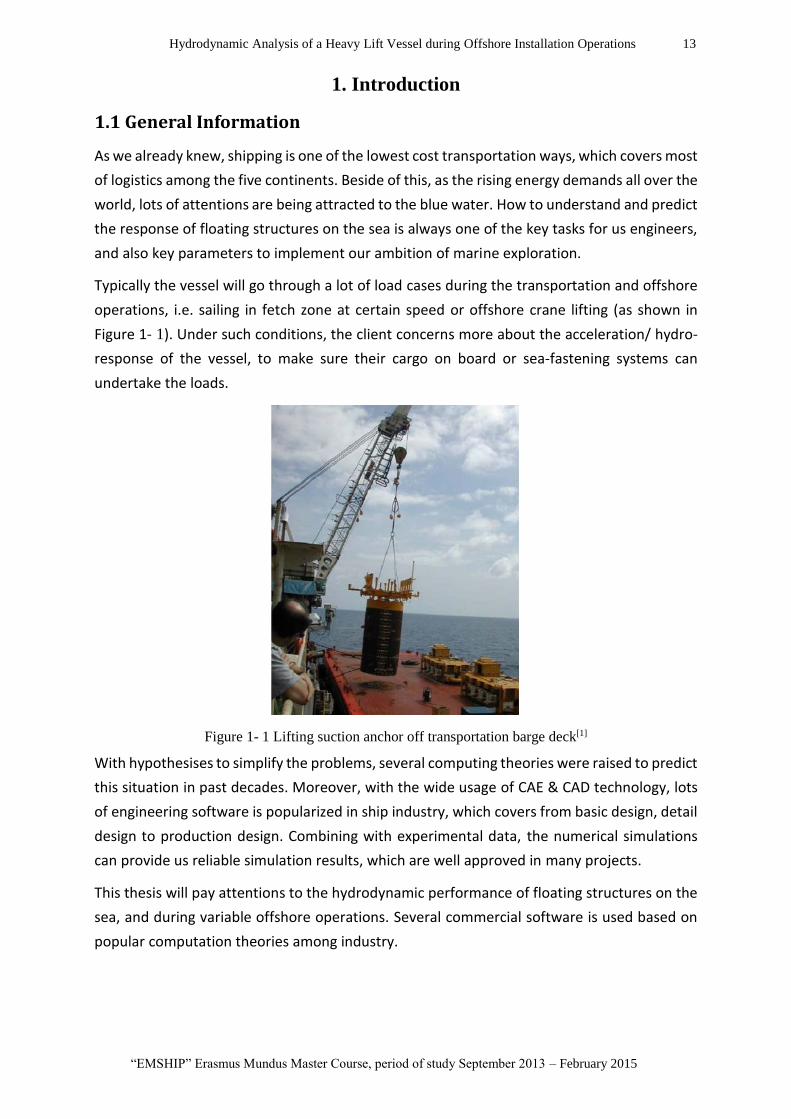
Typically the vessel will go through a lot of load cases during the transportation and offshore
operations, i.e. sailing in fetch zone at certain speed or offshore crane lifting (as shown in
Figure 1- 1). Under such conditions, the client concerns more about the acceleration/ hydro-
response of the vessel, to make sure their cargo on board or sea-fastening systems can
undertake the loads.
Figure 1- 1 Lifting suction anchor off transportation barge deck[1]
With hypothesises to simplify the problems, several computing theories were raised to predict
this situation in past decades. Moreover, with the wide usage of CAE & CAD technology, lots
of engineering software is popularized in ship industry, which covers from basic design, detail
design to production design. Combining with experimental data, the numerical simulations
can provide us reliable simulation results, which are well approved in many projects.
This thesis will pay attentions to the hydrodynamic performance of floating structures on the
sea, and during variable offshore operations. Several commercial software is used based on
popular computation theories among industry.

14 Bin Wang
Master Thesis developed at University of Rostock, Germany
1.2 Literature review for multi-body hydrodynamic problems
In many offshore operations, two or more closely positioned structures are used, with or
without connections between them. Over the years, multi-body hydrodynamic problems,
particularly two-body systems, have been investigated by researchers. Linear potential theory
has been widely used for this purpose and this requires that the following conditions are
satisfied: the fluid is incompressible, in-viscid, irrotational, and the motion of the structures
are small compared to their size. Three main numerical simulation methods based on the
linear potential theory have been developed for this use. These include the strip theory
method, the boundary integral method, and the finite element method[2],[3].
A. Strip theory method
Strip theory was developed for slender bodies which have one length-dimension substantially
greater than the others. In this case, it is assumed that the local force at one section of the
body is not affected by the shape of the other parts of the body. In a two body system, this
means that there is interaction only between the corresponding sections of the two structures.
After the strip theory was raised in 50’s, it was used on multi-body systems appeared about
one decade later. Kim[4] (1972) used the strip theory method to evaluate the hydrodynamic
forces and moments as well as the response motions of a twin-hull ocean platform in beam
seas. Ohkusu[5] (1969) calculated the hydrodynamic forces acting on two circular cylinders
connected with each other using the series expansion method and only heaving motion was
considered. In another of his paper[6] in 1974, the motions of a ship in the neighborhood of a
large moored two-dimensional floating structure was analyzed by strip theory. Based on his
results, we find that he clearly illustrated the effects of the position of a smaller body on the
weather and lee side against a large body. Kodan[7] (1984) extended Ohkusu’s method to
investigate the effects of hydrodynamic interaction between two parallel slender structures
in oblique waves and compared with the results from model experiments to support the
validity of the strip method, but the speed effect was not included.
B. Boundary integral method
Compared with the 2D-strip theory approach, the boundary integral method, which is also
known as panel method, can be used for ship hulls and ocean structures that have more
arbitrary geometries. Its formulation uses the Green’s theorem to express the velocity
potential in term of the surface distribution of singularities over the boundary surfaces which
are discretized into small panels. The wave exciting forces, the added mass and the damping
coefficients can be thus found, as well as the equations of motion.
Van Oortemerssen[8] (1979) was the first to apply the three dimensional source distribution
method, a common form of the Boundary Integral Method (BIM), for motion analysis of two
floating bodies with more arbitrary geometries. The numerical results showed good

Hydrodynamic Analysis of a Heavy Lift Vessel during Offshore Installation Operations 15
“EMSHIP” Erasmus Mundus Master Course, period of study September 2013 – February 2015
agreement with experimental data. However, he did not apply his method to ship
configurations and did not consider the speed effect either.
Loken[9] (1981) analyzed the wave-induced motions and wave-drifting forces and moments on
several close vessels in waves by a three-dimensional sink-source method, the results were
very satisfactory except for the resonance region. Duncan[ 10 ] et al. (1983) extended van
Oortmerssen’s technique to compute the coupled response of two ships, and the effects of
mooring lines and the cylindrical fenders were included. In his study, it was limited to the
conditions for two closely spaced ships with zero speed infinite depth water.
Inoue et al. [11] (1996) developed a general method for evaluating dynamic responses of
multiple-body systems having arbitrary connections. Linear stiffness matrices are introduced
into the equation of motions to represent the effect of the mooring lines and the connections.
These matrices are determined by the locations of the attachment points and the constant
stiffness of the connection. The case of a parallely connected FPSO unit and LNG carrier is
studied. The general analysis of the system only requires the frequency domain simulation.
But for detail analysis such as design of the connection, a time domain analysis should be
considered in order to take account of the nonlinear effects.
Fang and Chen(2001)[12] used three-dimensional source distribution method to predict the
relative motion and wave elevation between two bodies in waves. The corresponding Green
functions and their derivatives are solved by using the series expansions of Telste and
Noblesse’s algorithm for the Cauchy principal value integral of unsteady flow. The numerical
solution was compared with experimental data and strip theory, the results show that the
hydrodynamic interactions are generally important. In the resonance region, the
hydrodynamic interaction calculated by the 3D method is more reasonable.
J. N. Newman ‘s paper[13] reviews the extensive analytical and numerical accomplishments
when the number of bodies is very large, where asymptotic approximations are required. .
New computations are included to illustrate first-and second-order interaction effects. Special
consideration is given to configurations where the interactions are singular at certain
frequencies.
Hong and Kim et al.(2005)[ 14 ] used a higher-order boundary element method (HOBEM)
combined with generalized mode approach to analysis of motion and drift force of side-by-
side moored multiple vessels (LNG FPSO, LNGC and shuttle tankers). Model tests of global and
local motion responses and drift forces of three vessels are compared with numerical solutions.
C. Finite Element Method
Comparing with panel method, the advantage of the finite element method (FEM) is that it
can solve the problem that the solution of the surface integral equation is not unique at
irregular frequencies, which causes poor numerical conditioning.

16 Bin Wang
Master Thesis developed at University of Rostock, Germany
Taylor et al [15] used a combined method to analyze multi-component systems: FEM for fluid
region near the body and BIM for the far field region. It is an economical numerical technique
providing an accurate prediction of the hydrodynamic interaction between structures. The
formulation of the method was reviewed including the choice of element mesh, symmetry,
and equation solution. This method was applied to different multi-body configurations
including two horizontal cylinders, floating box & cylinder, and semi-submersible catamaran.
The comparison between the results obtained by the present method and those obtained by
using other methods gives a good agreement.
Min-Chih Huang et al. (1985)[ 16 ] developed a numerical procedure for predicting wave
diffraction, wave radiation, and body responses of multiple 3-D bodies of arbitrary shape was
described. Within the limits of linear wave theory, the boundary value problems are solved
numerically by the finite element method (FEM) using a radiation boundary damper approach.
Both permeable boundary dampers and a fictitious bottom boundary element are included in
the finite element algorithm in order to treat both permeable boundary problems and deep
water wave problems. Numerical results were presented for a variety of structures to illustrate
the following features: fictitious bottom boundary, multiple-structure wave interference, and
permeable boundary.
S.A. Sannasiraj et al. (2001)[17] used a two-dimensional numerical model to evaluate hydro-
dynamic coefficients and forces in an oblique wave field. It was found that the two-
dimensional model is applicable to investigate the wave-structure interaction problems of the
type herein considered.
Parallel to these numerical simulation methods, studies based on experimental results from
model tests present another view of the study of the two or multi-body system hydrodynamics,
especially for real industrial projects. For instance, the LNG FPSO/shuttle tanker system has
been widely investigated[18],[19].
1.3 Literature review for offshore crane lifting/lowering operations
Wagner (1932) first evaluated impact hydrodynamic loads on a body entering calm water,
which was applied to the problem of wave impact onto a vertical wall. The expression
provided good results for small dead rise angels[20]. This method was used by O. Faltinsen[21]
to develop a generalized Wagner’s based method (WBM) for solving the impact process of a
wave that reaches the deck at the front end of a platform and propagates downstream along
the length of the deck. Kaplan[22] (1993) raised method combining the momentum- and
drag- force analysis give a good prediction of the initial stages of the impact. am used
to determine the wave-induced loads acting on a ship in a seaway, including the effects on
hull girder loads due to slamming.
Rene Wouts’s article[23](1992) illustrated the significance of lift dynamic aspects observed
during two major offshore heavy lift operations performed in 1991. The contribution of lift

Hydrodynamic Analysis of a Heavy Lift Vessel during Offshore Installation Operations 17
“EMSHIP” Erasmus Mundus Master Course, period of study September 2013 – February 2015
dynamics to the overall response in the medium frequency range was found to be of similar
magnitude as the response in the wave frequency range. Initial correlation studies with
computer models show that this aspect was underestimated by the analyses.
Tim Bunnik[24],[25](2004) presented improved Volume Of Fluid (iVOF) method based on the
Navier-Stokes equations, was used to predict the behavior of a subsea structure in the splash
zone in ISOPE Conferences. Good initial comparison with model test shows the potential of
the iVOF method for the simulation of the behavior of subsea structures in the splash zone.
However, significant further development is needed before long simulations in irregular waves
can be carried out. Xiaozhou Hu (2014)[26] discretized the RANS equations by the finite volume
(FV) approach to track the complicated free surface, then numerical investigation of wave
slamming of flat bottom body during water entry process was done.
S.A. Reinholdtsen’s paper[ 27 ] (2003) presented some useful numerical force models for
simulation of multi-body offshore marine operations. The models cover pairs of docking
funnels and docking posts, bumper elements and fenders. A method for including n offshore
deck-mating operation/ time-varying mass was also covered. T.Jacobsen’s paper[28] outlined
the two methods for template installation, and states typical installation criteria based on
model tests and empirical data from full scale-measurements. Based on model tests, a
numerical hydrodynamic model was made of both methods and the typical design criteria
prior to the offshore operation were established, with the software SIMO.
J.L. Cozijn’s paper[29 ] (2008) described the analysis performed for the installation of two
topside modules by dynamically positioned S7000 crane vessel. The complete analysis
consisted of hydrodynamic scale model tests, time-domain simulations and observations
made during the actual installation offshore and the purpose of the analysis was to determine
the operational limits of the offshore installation. The computer simulations were carried out
using the multi-body time-domain simulation tool LIFSIM.
In K.P. Parkpaper’s paper[30 ] (2011), the dynamic factor was analyzed based on dynamic
simulations of a floating crane and a cargo, considering an elastic boom. Six-degree-of-
freedom motions were considered for the floating crane and for the cargo, and 3-dimensional
deformations for the elastic boom. The effects of the elastic boom on heavy cargo lifting were
discussed by comparing the simulation results of an elastic boom and a rigid boom. S.I.
Sagatun[31] suggested a new strategy for active control in heavy-lift offshore crane operations,
by introducing a new concept of wave synchronization in his article. Wave synchronization
reduces the hydrodynamic forces by minimization of variations in the relative vertical velocity
between payload and water using a wave amplitude measurement. Experimental results also
show that wave synchronization leads to significant improvements in performance.

18 Bin Wang
Master Thesis developed at University of Rostock, Germany
2. Hydrodynamic Problems under Potential Flow Theory
The domain of marine hydrodynamics includes applications of fluid mechanics which are
pertinent to ships, offshore platforms and other vessels. A variety of hydrodynamics problems
can be addressed within the context of potential flows, neglecting viscous effects. These
include the wave resistance of ships, motion of zero-speed ships and platform in waves, and
also the interactions between adjacent ships manoeuvring in close proximity. In these cases,
separation is avoid either because the geometry is streamlined, or because the Keulegan-
Carpenter (KC) number is small. Boundary-layer corrections can be applied when it is
appropriate to do so[32].
2.1 Potential flow theory
Equations of the potential flow problem to be stated here.
2.1.1 General equations in fluid domain
The governing equations in fluid mechanics, or wave mechanics are obtained using principles
and laws of classical physics, such as
- Conservation of mass which states that mass is neither created nor destroyed:
Equation of continuity:
∂
∂t𝜌 + ∇ ∙ (𝜌 ) = 0 (2-1)
For an incompressible-fluid flow, the equation of continuity reduces to:
∇ ∙ = 0 (2-2)
- Balance of momentum which is the same as the Newtons II Law which states that the rate of change of linear momentum of a body is equal to the sum of the external forces acting on the body:
Figure 2- 1 Force of pressure and gravity on fluid in region Ω bounded by surface S[33].
The rate of change of linear momentum of a system is equal to the sum of the external
forces acting on the system, we have:
∫∂ρu
∂tΩ
dΩ +∫ (ρu )u S
∙ n dS = −k ∫ ρgΩ
dΩ −∫ pnS
dS (2-3)

Hydrodynamic Analysis of a Heavy Lift Vessel during Offshore Installation Operations 19
“EMSHIP” Erasmus Mundus Master Course, period of study September 2013 – February 2015
Using Gauss integral identities and assuming that the flow variables are continuous, we
can simply equate the integrals:
u [∂ρ
∂t+ ∇ ∙ (ρu )] + ρ [
∂u
∂t+ (u ∙ ∇)u ] = −ρgk − ∇p (2-4)
By conservation of mass, above equation becomes:
𝜌 [∂
∂t+ ( ∙ ∇) ] = −∇(𝑝 + 𝜌𝑔𝑧) (2-5)
Equation (2-6) is well known as the Euler’s equations
- Balance of Linear Momentum in Viscous Fluid: The Incompressible Navier-Stokes Equation
Taking Euler’s equation as basis, we simply consider only the term that needs to be
modified to model effect of viscosity. Viscosity contributes to both normal and tangential
components of surface force. We define stress vector τ = σ ∙ n. One can show that
divσ = −∇𝑝 + 𝑢∇2 (2-7)
∇2 represents the Laplacian operator (eg., in Oxyz coordinates ∇2=∂2
∂x2+
∂2
∂y2+
∂2
∂z2 )
The equation of motion for the incompressible linear-viscous fluid flow, referred to as the
incompressible Navier-Stokes equations, are thus
ρ [∂u
∂t+ (u ∙ ∇)u ] = −ρgk − ∇p+ u∇2u (2-8)
The above equation is for the unknowns of u and pressure p.
2.1.2 Laplace equation.
A flow that is irrotational, inviscid and incompressible is called potential flow. In potential
flows the components of the velocity vector are no longer independent from each other. They
are coupled by the potential ∅. The derivative of the potential in arbitrary direction gives the
velocity component in this direction:
= 𝑢vw = ∇∅ (2-9)
Three unknowns (the velocity components) in above equation are thus reduced to one
unknown (the potential). This leads to a considerable simplification of the computation.
The continuity equation simplifies to Laplace’s equation for potential flow:
∆∅ = ∅𝑥𝑥 + ∅𝑦𝑦 + ∅𝑧𝑧 = 0 (2-10)
If the volumetric forces are limited to gravity forces, the Euler equations can be written as:
∇ [∅𝑡 +1
2(∇∅)2 − 𝑔𝑧 +
1
𝜌𝑝] = 0 (2-11)

20 Bin Wang
Master Thesis developed at University of Rostock, Germany
Integration gives Bernoulli’s equation:
∅𝑡 +1
2(∇∅)2 − 𝑔𝑧 +
1
𝜌𝑝 = 𝑐𝑜𝑛𝑠𝑡. (2-12)
The Laplace equation is sufficient to solve for the unknown velocities. From it, one can attempt
to solve for ∅, using given boundary conditions. Once ∅ is known, the pressure p in the flow
can also be found.
2.1.3 Solving the Laplace equation using singularity distributions
Sometimes it is very hard to solve the Laplace equation for given boundary conditions. Luckily
the Laplace equation is a linear differential equation. This offers the big advantage of
combining elementary solutions (so-called sources, sinks, dipoles, vortices) to arbitrarily
complex solutions. So let’s suppose that we have some solutions of the Laplace equation. Any
linear combination of these solutions will then also be a solution.
So the first thing we need to do is find some elementary solutions for the Laplace equation.
Examples of such solutions are sources, sinks, dipoles, vortices and such.
a. Sources and sinks
Now it is time to examine some elementary solutions. One such solution is the so-called source.
Let’s suppose we have a source with strength σ(Q), positioned at some point Q. The potential
∅ caused by this source at some point P then is
∅(𝑃) =𝜎(𝑄)
2𝜋ln (𝑟(𝑃, 𝑄)) (2-13)
By the way, if the source strength σ is negative, the source is often called a sink.
Figure 2- 2 Streamlines of the flow generated by a line source
We can put a lot of sources on a curve S. Then we get a source distribution. To find the velocity
potential at points P, caused by this distribution, we use an integral. This velocity potential
thus will be:

Hydrodynamic Analysis of a Heavy Lift Vessel during Offshore Installation Operations 21
“EMSHIP” Erasmus Mundus Master Course, period of study September 2013 – February 2015
∅(𝑃) = ∫𝜎(𝑄)
2𝜋ln (𝑟(𝑃, 𝑄))𝑑𝑠
𝑆
(2-14)
A problem might occur if the point P lies on the source distribution itself. Such a situation
should always be considered separately.
b. Doublets (Dipole)
Another elementary solution is the doublet. The potential at some point P, caused by a
doublet at Q, is given by
∅(𝑃) = 𝜇(𝑄)𝜕
𝜕𝑛𝑄(1
2𝜋ln(𝑟(𝑃, 𝑄))) (2-15)
Here µ(Q) is the strength of the doublet and 𝑛𝑄 is the direction of the doublet.
Figure 2- 3 Streamlines of the flow generated by a doublet line source aligned along the x-axis[34]
Once more, we can put a lot of doublets in a row. We then get a doublet distribution. To find
the velocity potential at P, we now have to use
∅(𝑃) = ∫ 𝜇(𝑄)𝜕
𝜕𝑛𝑄(1
2𝜋ln(𝑟(𝑃, 𝑄)))𝑑𝑠
𝑆
Once more, the case Q ∈ S should be considered separately.
2.2 General principle of the panel method
CFD comprises methods that solve the basic field equations subject to boundary conditions by
approaches involving a large number of (mathematically simple) elements. Here boundary
element methods (BEM) are used for potential flows.
For potential flows, the integrals over the whole fluid domain can be transformed to integrals
over the boundaries of the fluid domain. Therefore practical applications for potential flows
about ships (e.g. wave resistance problems) use exclusively BEM which are called panel
methods. Panel methods divide the surface of a ship (and often part of the surrounding water
surface) into discrete elements (panels). Each of these elements automatically fulfils the

22 Bin Wang
Master Thesis developed at University of Rostock, Germany
Laplace equation. Indirect methods determine the element strengths so that at the collocation
points (usually centres of the panels) a linear boundary condition (e.g. zero normal velocity) is
fulfilled. This involves the solution of a full system of linear equations with the source
strengths as unknowns.
The required velocities are computed in a second step, hence ‘indirect’ method. Bernoulli’s
equation yields then the pressure field. Direct methods determine the potential directly. They
are less suited for boundary conditions involving higher derivatives of the potential, but yield
higher accuracy for lifting flows. Most commercially used codes for ship flows are based on
indirect methods. BEM cannot be used to solve RANSE. Fundamentals of BEM can be found
in, e.g., Hess (1990)[35].
2.2.1 Diffraction Theory
According to linear potential theory, the potential of a floating body is a superposition of the
potentials due to the undisturbed incoming wave ∅𝐼 , the potential due to the diffraction of
the undisturbed incoming wave on the fixed body ∅𝑑 and the radiation potentials due to the
six body motions ∅𝑗:
Φ=∑ ∅𝑗 +6𝑗=1 ∅𝐼 + ∅𝑑 (2-16)
Again, the fluid is assumed to be incompressible, inviscid and irrotational, without any effects
of surface tension. The motion amplitudes and velocities are small enough. The potentials
have to satisfy following boundary conditions:
• 1. Laplace equation The continuity condition or Laplace equation holds in the fluid domain:
𝜕∅2
𝜕𝑥2+𝜕∅2
𝜕𝑦2+𝜕∅2
𝜕𝑧2= 0 (2-17)
• 2. Sea bed boundary condition At the sea bed:
𝜕∅
𝜕𝑧= 0 𝑤𝑖𝑡ℎ 𝑧 = −ℎ0 (2-18)
In which ℎ0 is the distance from the origin of the earth-bound coordinate system O(x; y;
z), to the sea bed. Note that, in contrast to the earlier theory, this treatment is for water
with a finite depth.
• 3. Free surface boundary condition At the mean free surface:
𝑔𝜕∅
𝜕𝑧+𝜕∅2
𝜕𝑡2= 0 (2-19)
• 4. Kinematic boundary condition on the oscillating body surface On the wetted part of the oscillating hull of the structure (in its mean position):

Hydrodynamic Analysis of a Heavy Lift Vessel during Offshore Installation Operations 23
“EMSHIP” Erasmus Mundus Master Course, period of study September 2013 – February 2015
𝜕∅
𝜕𝑛= 𝑣 ∙ (2-20)
In which 𝑣 is the velocity of a point on the hull of the body and is the normal vector of
the hull, positive into the fluid.
• 5. Radiation condition The body motion and diffraction potentials have to satisfy a radiation condition that at
great distance from the body these potentials disappear. This condition imposes a
uniqueness that would not otherwise be presented; such discussions are found in
(Oortmerssen, 1976)[36].
The free-surface condition follows from the assumptions that the pressure at the surface is
constant and that water particles do not pass through the free surface. The condition on the
wetted surface of the body assures the no-leak condition of the (oscillating) hull. The condition
at the sea bed is also a no-leak condition.
The boundary conditions are generated and apply to all possible realizations of wave
conditions. Here the theory is developed for a unidirectional regular wave. Superposition can
be used to study all sorts of irregular wave conditions - even those with directional spreading.
In regular waves a linear potential Φ, which is a function of the earth-fixed coordinates and of
time t, can be written as a product of a space-dependent term and a harmonic time-
dependent term as follows
Φ(x, y, z; t) = ∅(x, y, z) ∙ 𝑒−𝑖𝜔𝑡 (2-21)
The boundary conditions for the potential, Φ , result in similar conditions for the space
dependent term, ∅.
In the case of long crested, harmonic progressive waves the incident potential (space-
dependent part of the velocity potential) for finite depth (h), is defined as:
∅𝐼 =−𝑖𝑔𝜉0𝜔
cosh [𝑘(𝑧 + ℎ)]
cosh 𝑘ℎ𝑒𝑖𝑘(𝑥𝑐𝑜𝑠𝜒+𝑦𝑠𝑖𝑛𝜒) (2-22)
in which :
𝜉0 = amplitude of undisturbed wave
k=2π/λ = wave number
λ = wave length
h = water depth
g = acceleration of gravity
𝜒 = angle between incident waves and X axis
The individual potentials should satisfy the Laplace equation in the fluid domain. There are
different solutions for above Laplace equation and the boundary conditions of the problem

24 Bin Wang
Master Thesis developed at University of Rostock, Germany
specify the suitable solution for each problem. The fluid pressure follows from Bernoulli
equation:
𝑝(𝑥, 𝑦, 𝑧; 𝑧) = −𝜌𝜕∅
𝜕𝑡 = ρω2 (∅𝐼 + ∅𝑑)𝜁0 + ∑ ∅𝑗𝜁𝑗 ∙ 𝑒
−𝑖𝜔𝑡6𝑗=1 (2-23)
However, there is no analytical solution for diffraction potential ∅𝑑 and radiation potentials
∅𝑗, so the problem should be solved numerically.
2.2.2 Solving Potentials (Green’s Function Method)
According to the 3-D source method, the potentials ∅𝑑 and ∅𝑗 can be expressed in terms of
well-known Green functions.
The Green’s functions G with its first and second derivatives are continuous everywhere
except at the point q(, , ). It can be interpreted as the response of a system at a field point
p(x, y, z) due to a delta function input at the source point q(, , ). This can be applied with
the Green’s second theorem to derive the integral equation for the velocity potentials on the
surface of the body:
2π∅(𝑝) +∬∅(𝑞)𝜕𝐺(𝑝, 𝑞)
𝜕𝑛(𝑞)𝑑𝑆𝑞 =
𝑆
∬G(p, q)𝜕∅(𝑞)
𝜕𝑛(𝑞)𝑑𝑆𝑞
𝑆
(2-24)
Alternately, the more compact integral equation may be used to obtain ∅𝑑 on the surface of
the body:
4π∅𝐷(𝑝) +∬∅𝐷(𝑞)𝜕𝐺(𝑝, 𝑞)
𝜕𝑛(𝑞)𝑑𝑆𝑞 =
𝑆
4π∅𝐼(𝑝) (2-25)
As a result, boundary conditions are reduced only to wetted surfaces of the body[37].The
integral equation is solved numerically by a panel method in which the body surface is
approximated by an ensemble of flat quadrilateral panels and the value of the potential is
assumed to be constant over each panel. Utilizing a collocation method in which the integral
equation is satisfied at one point for each panel, the problem is reduced to solving a linear
system for the values of the velocity potential strengths on each panel.
According to [Lamb, 1932][38], the potential ∅𝑗 at a point (x, y, z) on the mean wetted body
surface 𝑆0 due to a motion in the mode j (j = 1 to 6) and the diffraction potential ∅𝐷 can be
represented by a continuous distribution of single sources on the body surface:
∅𝑗(𝑥, 𝑦, 𝑧) =1
4𝜋∬𝜎𝑗(, , ) ∙ 𝐺
𝑆0
(𝑥, 𝑦, 𝑧, , , ) ∙ 𝑑𝑆0
𝑓𝑜𝑟 𝑗 = 1,… 7
(2-26)
in which:
• ∅𝑗(𝑥, 𝑦, 𝑧) is the potential function in a point (x, y, z) on the mean wetted body surface,
𝑆0 . The cases with j = 1, ..6 correspond to the potentials due to a motion of the body

Hydrodynamic Analysis of a Heavy Lift Vessel during Offshore Installation Operations 25
“EMSHIP” Erasmus Mundus Master Course, period of study September 2013 – February 2015
in the j𝑡ℎ mode, while ∅7 (or ∅𝑑 ) is the potential of the diffracted waves. The
individual potentials satisfy all boundary conditions.
• 𝜎𝑗(, , ) is the complex source strength in a point (, , ) on the mean wetted body
surface 𝑆0, due to a motion of the body in the j -mode.
• 𝐺(𝑥, 𝑦, 𝑧, , , ) is the Green’s function of the pulsating source 𝜎𝑗(, , ) in a point
located at (, , ) on the potential ∅𝑗(𝑥, 𝑦, 𝑧) in a point located at (x, y, z), singular for
(, , ) = (x, y, z).
This Green’s function satisfies the Laplace equation, the linearized boundary conditions on
the seabed and on the free surface and the radiation condition at infinity.
According to [Wehausen and Laitone, 1960][39]:
𝐺(𝑥, 𝑦, 𝑧, , , ) = 1
𝑟+1
𝑟1
+𝑃𝑉∫2(𝑘 + 𝑣)𝑒−𝑘ℎ ∙ cosh 𝑘(ℎ0 + ) ∙ cosh 𝑘(ℎ0 + 𝑧)
𝑘𝑠𝑖𝑛ℎ(𝑘ℎ) − 𝑣𝑐𝑜𝑠ℎ(𝑘ℎ)
∞
0
∙ 𝐽0(𝑘𝑅) ∙ 𝑑𝑘
+i ∙2𝜋(𝑘2 − 𝑣2) ∙ 𝑐𝑜𝑠ℎ 𝑘(ℎ0 + ) ∙ 𝑐𝑜𝑠ℎ 𝑘(ℎ0 + )
(𝑘2 − 𝑣2)ℎ − 𝑣∙ 𝐽0(𝑘𝑅) (2-27)
This free-surface Green’s function satisfies all boundary conditions except the body
surface boundary condition[40].
Furthermore, according to [John, 1949][41]:
𝐺(𝑥, 𝑦, 𝑧, , , )
= 2𝜋𝑣2 − 𝑘2
(𝑘2 − 𝑣2)ℎ + 𝑣∙ cosh 𝑘(ℎ0 + ) ∙ cosh 𝑘(ℎ0 + 𝑧) ∙ 𝑌0(𝑘𝑟) − 𝑖𝐽0(𝑘𝑅)
+∑4(𝑘𝑖
2+𝑣2)
(𝑘𝑖2+𝑣2)ℎ−𝑣
∙ cosh 𝑘𝑖(ℎ0 + ) ∙ cosh 𝑘𝑖(ℎ0 + 𝑧) ∙ 𝐾0(𝑘𝑖𝑅)∞𝑖=1 (2-28)
In which
r = √(𝑥 − )2 + (𝑦 − )2 + (𝑧 − )2
r1 = √(𝑥 − )2 + (𝑦 − )2 + (𝑧 + 2ℎ0 + )2 (= mirrored)
R = √(𝑥 − )2 + (𝑦 − )2
J0, K0 and 𝑌0 = Bessel functions
𝑣 = 𝜔2/𝑔
𝑘𝑖 = 𝑝𝑜𝑠𝑖𝑡𝑖𝑣𝑒 𝑠𝑜𝑙𝑢𝑡𝑖𝑜𝑛𝑠 𝑜𝑓 tanh(𝑘𝑖ℎ) + 𝑣 = 0
These two representations are equivalent. In general, equation (2-27) is the most convenient
representation for calculations, but when R = 0 the value of K0 becomes infinite, so that
equation (2-28) must be used when R is small or zero. Meanwhile computation involving both
formulations can be speeded up through the use of polynomial expressions, see Newman[42].

26 Bin Wang
Master Thesis developed at University of Rostock, Germany
As mentioned before, the unknown source strengths 𝜎𝑗(, , ) are determined based on the
normal velocity boundary condition on the body:
∂∅𝑗
∂x 𝑗= 𝑛𝑗 (2-29)
= −1
2𝜎𝑗(𝑥, 𝑦, 𝑧) +
1
4𝜋∬𝜎𝑗(, , ) ∙
𝜕𝐺(𝑥, 𝑦, 𝑧, , , )
𝜕𝑛𝑆0
∙ 𝑑𝑆0 𝑓𝑜𝑟 𝑗 = 1,… 6
In the above equations, the operator ∂
∂n signifies the gradient in the direction of the normal
to the surface of the body.
Finally, the motions ζ𝑗 are determined from the solution of the following coupled equations
of motion for six degrees of freedom:
∑−𝜔2(𝑚𝑘𝑗 + 𝑎𝑘𝑗) − 𝑖𝜔𝑏𝑘𝑗
6
𝑗=1
+ 𝑐𝑘𝑗 ∙ ζ𝑗 = X𝑘 𝑓𝑜𝑟 𝑘 = 1, . .6 (2-30)
With:
𝑚𝑘𝑗 = inertia matrix of the body for inertia coupling in the k-mode for acceleration in the
j-mode.
𝑎𝑘𝑗 =inertia matrix of the body for inertia coupling in the k-mode for acceleration in the
j-mode.
𝑏𝑘𝑗 =damping matrix for the force on the body in the k-mode due to velocity of the body
in the j-mode.
𝑐𝑘𝑗 =spring matrix for the force on the body in the k-mode due to motion of the body in
the j-mode.
Xk = wave force on the body in the k-mode.
2.3 Method of Singularities of Rankine for Seakeeping Problem
The choice of the most appropriate Green’s function is particular to each boundary problem[43].
In the context of seakeeping problems there are some famous ones, such as the transient
Green function, Kelvin sources and Rankine sources, this last one being discussed here.
The Rankine panel method distributes sources on the free surface as on the body surface. The
Green function method only distributes source on the body surface, because the Green
function automatically satisfies the linearized free-surface condition.
Two problems have long impeded the application of Rankine source methods to free-surface
flows[44]:
- The radiation condition: In the steady wave problem, wave will propagate only
downstream; i.e. far ahead of the ship no waves may appear.

Hydrodynamic Analysis of a Heavy Lift Vessel during Offshore Installation Operations 27
“EMSHIP” Erasmus Mundus Master Course, period of study September 2013 – February 2015
- The open-boundary condition: only a limited area of the free surface can be discretized.
Waves must pass through the outer boundary of this area without significant reflection.
Both conditions must be fulfilled numerically. Here the computation in frequency domain to
be discussed.
A Cartesian coordinate system O-xyz is employed to compute the wave interaction with a
floating body at forward speed, U. The oxy plane is on the plane with z=0 which represents
the undisturbed water surface. The z-axis is the positive upward. Incident waves propagate at
an angle β relative to the x-axis.
Figure 2- 4 Typical Discretized Panel Elements Using Rankine Source Method. (Source: Muniyandy
Elangovan, Indian Register of Shipping, India)
A ship with smooth surface moves with uniform speed U in a homogeneous, incompressible
and inviscous fluid, which is only bounded by the ship’s hull and the free surface. The set of
equations defining the problem of singularities of Rankine is the following:
∆∅ = 0 𝑖𝑛 (𝐷), 𝐿𝑎𝑝𝑙𝑎𝑐𝑒 𝐸𝑞𝑢𝑎𝑡𝑖𝑜𝑛
(𝜕∅
𝜕𝑛)𝑐= 0, 𝑆𝑙𝑖𝑝 𝐶𝑜𝑛𝑑𝑖𝑡𝑖𝑜𝑛
𝐸 ∅ = 0|𝑧=0 𝑜𝑛 𝑆𝐿𝑚, 𝑚𝑒𝑠ℎ𝑒𝑑 𝑝𝑎𝑟𝑡 𝑜𝑓 𝑡ℎ𝑒 𝑓𝑟𝑒𝑒 𝑠𝑢𝑟𝑓𝑎𝑐𝑒 (𝑆𝐿).
𝜕∅
𝜕𝑧= 0|
𝑧=0 𝑜𝑛 𝑆𝐿, 𝑛𝑜𝑛 𝑚𝑒𝑠ℎ𝑒𝑑 𝑝𝑎𝑟𝑡 𝑜𝑓 𝑡ℎ𝑒 𝑓𝑟𝑒𝑒 𝑠𝑢𝑟𝑓𝑎𝑐𝑒 (𝑆𝐿)
∅ → 𝑈𝑥 𝑎𝑡 𝑖𝑛𝑓𝑖𝑛𝑖𝑡𝑦,
(2-31)
In which, E is linearized free surface boundary operator (see Neuman-Kelvin or Dawson
theory)[45]. By applying the free surface operator E to the 3rd Green’s fuction, we can verify
the condition of symmetry on 𝑆𝐿,.
The total velocity potential at field point p(x, y, z) is assumed to be time harmonic:

28 Bin Wang
Master Thesis developed at University of Rostock, Germany
Ф(𝑝) = −𝑈𝑥 + 𝑈∅ + 𝑅𝑒[∑𝜁𝑗∅𝑗𝑒−𝑖𝜔𝑡
7
𝑗=0
] (2-32)
∅ is the steady potential due to unit forward speed; ∅0 is the incident wave potential (equal
to ∅𝐼 we used before ) while ∅7 is the diffracted wave potential (or ∅𝐷 we used before ).
∅𝑗 𝑓𝑜𝑟 𝑗 = 1,… 6 are the radiation potentials with respect to motions in six degrees of
freedom; 𝜁𝑗 𝑓𝑜𝑟 𝑗 = 1, …6 are the motion amplitudes; 𝜁0 = 𝜁7 is the incident amplitude; and
𝜔 is the frequency of encounter.
The radiation and the diffraction potentials for a body with forward speed are computed from
de-singularized integrals in terms of source strength by using the forward-speed Green
function in the frequency domain. For detail, see [Volker Bertram, 1990] or [Qiu, 2007][46][47].
2.4 Frank’s Method of Pulsating Sources: a 2-D Strip Theory
Strip theory is valid for long and slender bodies only. In spite of this restriction, experiments
have shown that strip theory can be applied successfully for floating bodies with a length to
breadth ratio L/B ≥ 3, , at least from a practical point of view[48].
2.4.1 Basic concept of strip theory
Strip theory considers a ship to be made up of a finite number of transverse two-dimensional
slices, which are rigidly connected to each other. Each slice is treated hydrodynamically as if
it is a segment of an infinitely long floating cylinder.
Figure 2- 5 A picked slice within strip theory[49]
All waves which are produced by the oscillating ship (hydro-mechanic loads) and the diffracted
waves (wave loads) are assumed to travel parallel to the (y, z)-plane of the ship. The fore and
aft side of the body (such as a pontoon) does not produce waves in the x -direction. For zero
forward speed case, interactions between the cross sections are ignored.
2.4.2 Frank’s Method of Pulsating Sources
The two-dimensional nature of the strip problem implies three degrees of freedom of motion:

Hydrodynamic Analysis of a Heavy Lift Vessel during Offshore Installation Operations 29
“EMSHIP” Erasmus Mundus Master Course, period of study September 2013 – February 2015
• Vertical or heave,
• Horizontal or sway and
• Rotational about a horizontal axis or roll.
Within boundary value problem of potential theory, the cylinder is forced into harmonic
motion 𝐴(𝑚) ∙ cos (ω ∙ t) with a prescribed radian frequency of oscillation ω, where the
superscript 𝑚 may take on the values 2, 3 and 4, denoting swaying, heaving and rolling
motions, respectively.
According to Green’s function (see Equ.2-27), the real point-source potential can be written
as[49]:
H(x, 𝑦; , ; 𝑡) = 𝑅𝑒𝐺(𝑧, 𝜁, 𝑡) (2-33)
Where
𝐺(𝑝, 𝑞, 𝑡) is the Green’s function of the pulsating source 𝜎𝑗(, , 𝑡) in a point located
at ζ(, ) on the potential ∅𝑗(𝑥, 𝑦, 𝑡) in a point located at z(x, y), singular for ζ(, ) =
z(x, y).
Letting:
G(z, ζ) =1
2π∙ 𝑅𝑒 ln(𝑧 − ζ) − ln(z − ζ) + 2 ∙ PV∫
𝑒−𝑖∙𝑘∙(𝑧−ζ)𝜋
𝑣 − 𝑘
∞
0
𝑑𝑘
−𝑖 ∙ 𝑅𝑒𝑒−𝑖∙𝑣∙(𝑧−ζ) (2-34)
where
𝑧 = 𝑥 + 𝑖 ∙ 𝑦; ζ = + 𝑖 ∙ ; ζ = − 𝑖 ∙ ; 𝑣 = 𝜔2/𝑔
Then we have:
H(x, 𝑦; , ; 𝑡) = 𝑅𝑒𝐺(𝑧, 𝜁, 𝑡) ∙ 𝑒−𝑖𝜔𝑡 (2-35)
This equation satisfies Laplace equation, the boundary conditions and alsothe radiation
condition,
Ф(𝑚)(𝑥, 𝑦, 𝑡) = 𝑅𝑒∫ 𝑄(𝑠) ∙ G(z, ζ) ∙ 𝑒−𝑖𝜔𝑡 ∙ 𝑑𝑠𝐶0
, (2-36)
Where
𝐶0 is the submerged contour of the cylindrical cross section at its mean (rest) position and 𝑄(𝑠) represents the complex source density as a function of the position along 𝐶0 .
Application of the kinematic boundary condition on the oscillating cylinder at z(x,y) yields:
𝑅𝑒( ∙ ∇ ) ∙ ∫ 𝑄(𝑠) ∙ G(z, ζ) ∙ 𝑑𝑠𝐶0
= 0 (2-37)
𝐼𝑚( ∙ ∇ ) ∙ ∫ 𝑄(𝑠) ∙ G(z, ζ) ∙ 𝑑𝑠𝐶0
= 𝐴(𝑚) ∙ 𝜔 ∙ 𝑛(𝑚) (2-38)

30 Bin Wang
Master Thesis developed at University of Rostock, Germany
Where:
𝐴(𝑚) denotes the amplitude of oscillation and 𝑛(𝑚) the direction cosine of the normal
velocity at z(x,y) on the cylinder. Both 𝐴(𝑚)and 𝑛(𝑚) depend on the mode of motion of the cylinder.
Above equations are applied at the midpoints of each of the N segments and it is assumed
that over an individual segment the complex source strength 𝑄(𝑠) remains constant, although
it varies from segment to segment. With these stipulations, this set of coupled integral
equations (2-37) & (2-38) becomes a set of 2*N linear algebraic equations in the unknowns:
𝑅𝑒𝑄(𝑚)(𝑠𝑗) = 𝑄𝑗(𝑚) 𝑎𝑛𝑑 𝐼𝑚𝑄(𝑚)(𝑠𝑗) = 𝑄𝑁+𝑗
(𝑚) (2-39)
Thus, for i=1,2,…,N:
+∑𝑄𝑗(𝑚) + 𝐼𝑖𝑗
(𝑚)
𝑁
𝑗=1
+∑𝑄𝑁+𝑗(𝑚) + 𝐽𝑖𝑗
(𝑚)
𝑁
𝑗=1
= 0 (2-40)
−∑𝑄𝑗(𝑚) + 𝐽𝑖𝑗
(𝑚)
𝑁
𝑗=1
+∑𝑄𝑁+𝑗(𝑚) + 𝐼𝑖𝑗
(𝑚)
𝑁
𝑗=1
= 𝜔 ∙ 𝐴(𝑚) ∙ 𝑛𝑖(𝑚) (2-41)
Where the superscript 𝑚 denotes the mode of motion.
The hydrodynamic pressure at (x𝑖, 𝑦𝑖) along the cylinder is obtained from the velocity
potential by means of the linearized Bernoulli equation:
𝑝(𝑚)(x𝑖, 𝑦𝑖, 𝜔, 𝑡) = −𝜌 ∙𝜕Ф(𝑚)
𝜕𝑡(x𝑖, 𝑦𝑖 , 𝜔, 𝑡) (2-42)
And:
𝑝(𝑚)(x𝑖, 𝑦𝑖, 𝜔, 𝑡)
= 𝑝𝑎(𝑚)(x𝑖, 𝑦𝑖 , 𝜔) ∙ cos(𝜔 ∙ 𝑡) + 𝑝𝑣
(𝑚)(x𝑖 , 𝑦𝑖 , 𝜔) ∙ sin(𝜔 ∙ 𝑡) (2-43)
where 𝑝𝑎(𝑚) and 𝑝𝑣
(𝑚) are the hydrodynamic pressure in-phase with the displacement and in-
phase with the velocity, respectively.
Hydrodynamic Analysis of a Heavy Lift Vessel during Offshore Installation Operations 31
“EMSHIP” Erasmus Mundus Master Course, period of study September 2013 – February 2015
3. Comparative Study on Seakeeping Codes
3.1 Introduction
The prediction of ship motions, resistance, and dynamic effects like deck wetness and
slamming in a realistic seaway is very important during each shipping, heavy-lift transportation
and offshore operations. This makes seakeeping very essential.
The direct and practical way to obtain the seakeeping result is to run model test. The results
gained are very accurate, but the process is costly and time-consuming and seakeeping tank
test is not affordable in most of realistic projects. An alternative and popular way nowadays,
is to adopt computer codes to do the seakeeping prediction work. However, different
software may provide different results under same environmental condition. Here introduce
several software that will be involved in following comparisons.
GL-Rankine is a sea-keeping program that is developed by DNV-GL. The code calculates the 6-
DOF motions of the ship (surge, sway, heave, roll, pitch and yaw), the motions and
accelerations of specified points located on the hull, as well as the wave induced loads (forces
and moments) at specified ship sections. In addition, the code delivers the hydrodynamic
pressures along the wetted surface of the freely moving body hull, in response to a regular
incident wave train. The program GL-Rankine can be used for the following computations[50]:
• Resistance in calm water, taking into account shallow water and channel walls
• Dynamic squat in calm water, taking into account shallow water and channel walls
• Linear transfer functions of ship motions in regular waves
• Sectional loads, relative motions and accelerations in waves
• Mapping of pressure distributions onto nodes of a finite-element mesh
• Hydrodynamic interaction of ships with the same forward speed and course
WASIM is a hydrodynamic program for computing global responses and local loading on
vessels moving at any forward speed. The simulations are carried out in the time domain, but
results are also transformed to the frequency domain using Fourier transformations. WASIM
solves the fully 3-dimensional radiation/diffraction problem by a Rankine panel method[51].
OCTOPUS is a hydrodynamic analysis program for the calculation of seakeeping characteristics
of ships and other floating structures, with or without forward speed. Using the linear 2D strip
method, OCTOPUS can calculate site or voyage dependent response statistics and create 2D
hydrodynamic databases[52].
3.2 Scope of Work
The comparisons are selected such that they covered a range of different methods:
Non-Linear Steady Cases: Linear potential methods linearizing around the non-linear
steady wave field.

32 Bin Wang
Master Thesis developed at University of Rostock, Germany
Approximate Forward Speed Cases: Linear potential method linearizing around the
undisturbed flow, applying zero-speed Green Functions.
2-D Strip Method Cases: Linear potential method linearizing around transverse two
dimensional slices, then 3-DOF results are extended to global responses.
In this chapter, typical heavy lift vessel (HLV) hulls are used in the comparative study. In
general, the main works including:
a. Use GL-Rankine to calculate the hydrodynamic response for both zero speed case
and certain forward speed cases, applying with different theories.
b. Compare those results with hydrodynamic database from the other software
(analyzed with WASIM, or OCTPUS). The comparisons are conducted for a wide range
of wave periods and wave heading angles.
Airy wave theory is used for all load cases.
No viscous damping was considered into all analyzed conditions, which means only potential
damping to be conducted. As you can image, no wind or current is considered in analysis, in
order to exclude the possible deviation from this.
3.3 General Information of Comparison Models
3.3.1 Coordinate system
An orthogonal, right-handed coordinate system (x-axis forward, z-axis upward) is used, as
shown in Figure 3- 1. The z=0 plane is placed on undisturbed water plane.
Figure 3- 1 Ship motion with 6 degrees of freedom (Source : Internet)
3.3.2 Description of hull form Discretization
For the numerical validation, the wetted surface of vessel hull is discretized (see Figure 3- 2)
with affordable mesh size. The total number of panel elements on body surface is around
2000~4000, depending on variable cases.

Hydrodynamic Analysis of a Heavy Lift Vessel during Offshore Installation Operations 33
“EMSHIP” Erasmus Mundus Master Course, period of study September 2013 – February 2015
Figure 3- 2 Surface discretization of a ship hull in GL-Rankine
In each case, the ship is considered to encounter a regular wave, defined by its parameters:
• wave length λ or period T
• heading angle α (counterclockwise angle with x-axis. see Figure 3- 3)
• wave height (double amplitude)
• wave phase (see following Figure 3- 3).
Figure 3- 3 Wave heading setting
The wave length λ and wave period T are linked by the following relation: λ = g ∙ T2/2𝜋 ,
which means infinite water depth condition is assumed during the seakeeping simulations.
3.4 Zero-Speed Cases: Hydrodynamic Analysis using Green Function
The following table shows the basic dimensions and characteristics of the selected ‘Type I’
vessel shown in Figure 3- 2, which will be used in following numerical simulations. No trim or
heel angle is assumed under hydrostatic status.
Table 3- 1 ‘Type I’ Vessel Parameters
TYPE Lpp
/m
Beam
/m
Depth
/m
Draft
/m
Displacement/
Mt
GMt
/m
Number of Total
Panels
Hull
Type I 149.4 27.5 13.8 8.2 20770 4.76
2700-4000, depends
on cases

34 Bin Wang
Master Thesis developed at University of Rostock, Germany
For zero speed cases, computations are done firstly in the frequency domain by GL-Rankine,
using the linear Neumann-Kelvin approach in which the body boundary condition is applied
on the mean position of the exact body surface and linearized free surface boundary
conditions are fulfilled. These assumptions allow solutions to take Green Function technique
to solve 3-D radiation potential problems. An internal boundary inside the body may be
needed to eliminate irregular frequencies in some cases.
Three different wave-heading angles (α=00, 600, and 900 ) are considered here. Those results
obtained from GL-Rankine are compared with the well-approved database from a third party,
which was obtained with DNV/WASIM software and are already well-approved in finished
projects. Here some typical comparative results are given:
(a)
(b)

Hydrodynamic Analysis of a Heavy Lift Vessel during Offshore Installation Operations 35
“EMSHIP” Erasmus Mundus Master Course, period of study September 2013 – February 2015
(c)
(d)
(e)
36 Bin Wang
Master Thesis developed at University of Rostock, Germany
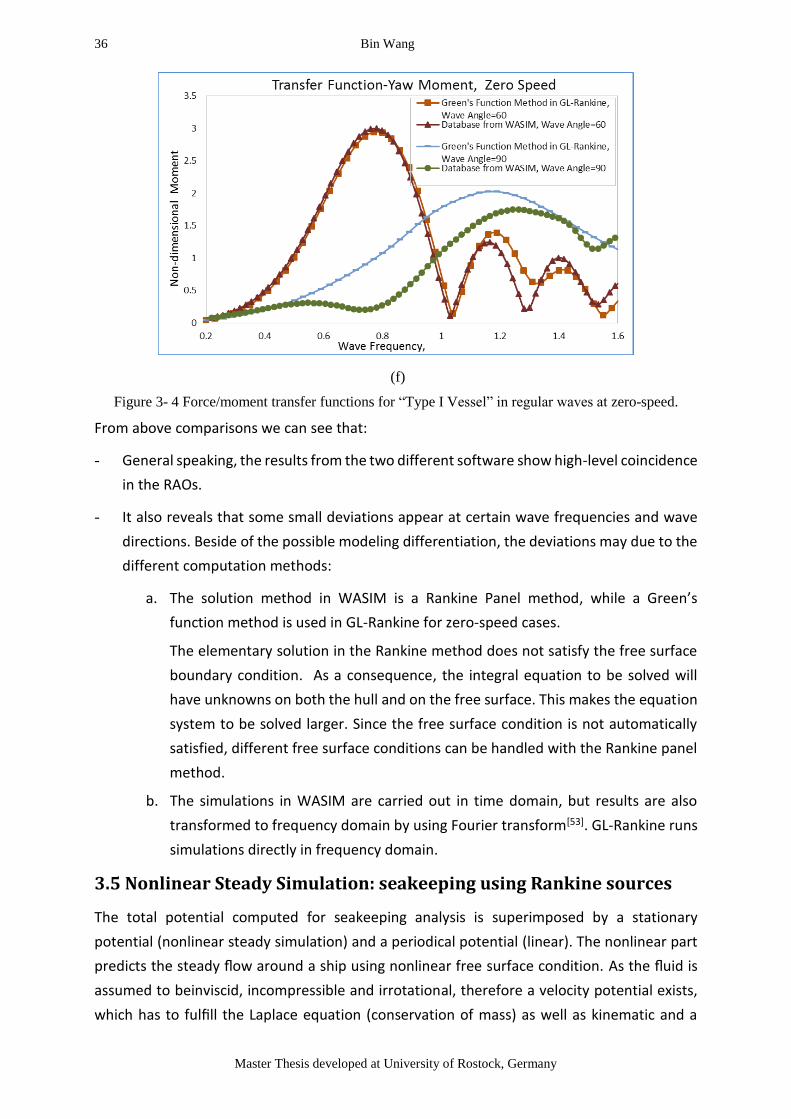
(f)
Figure 3- 4 Force/moment transfer functions for “Type I Vessel” in regular waves at zero-speed.
From above comparisons we can see that:
- General speaking, the results from the two different software show high-level coincidence
in the RAOs.
- It also reveals that some small deviations appear at certain wave frequencies and wave
directions. Beside of the possible modeling differentiation, the deviations may due to the
different computation methods:
a. The solution method in WASIM is a Rankine Panel method, while a Green’s
function method is used in GL-Rankine for zero-speed cases.
The elementary solution in the Rankine method does not satisfy the free surface
boundary condition. As a consequence, the integral equation to be solved will
have unknowns on both the hull and on the free surface. This makes the equation
system to be solved larger. Since the free surface condition is not automatically
satisfied, different free surface conditions can be handled with the Rankine panel
method.
b. The simulations in WASIM are carried out in time domain, but results are also
transformed to frequency domain by using Fourier transform[53]. GL-Rankine runs
simulations directly in frequency domain.
3.5 Nonlinear Steady Simulation: seakeeping using Rankine sources
The total potential computed for seakeeping analysis is superimposed by a stationary
potential (nonlinear steady simulation) and a periodical potential (linear). The nonlinear part
predicts the steady flow around a ship using nonlinear free surface condition. As the fluid is
assumed to beinviscid, incompressible and irrotational, therefore a velocity potential exists,
which has to fulfill the Laplace equation (conservation of mass) as well as kinematic and a

Hydrodynamic Analysis of a Heavy Lift Vessel during Offshore Installation Operations 37
“EMSHIP” Erasmus Mundus Master Course, period of study September 2013 – February 2015
dynamic boundary conditions on the free surface. Because the free surface boundary
condition is non-linear an iterative solution is required. An under relaxed Newton-like iteration
for the residuum is used.
Comparing with more-time consuming CFD simulations with RANSE method, the Rankine
source method can provide a high-level seakeeping prediction within shorter time, as shown
in Figure 3- 5.
Figure 3- 5 Wave Pattern using Rankine sources (upper half) vs RANSE-based method (bottom).
(Source of photo: Dipl.-Ing. Alexander von Graefe)
3.5.1 Free surface generation
To fulfill the linear free surface condition, GL-Rankine needs panels on the free surface. The
grid consists of an inner free surface grid with the same structure as the grid for nonlinear
steady computation, and an outer free surface grid. The outer grid is coarser than the inner
grid as shown in Figure 3- 6; a different boundary condition is fulfilled on the outer grid to
prevent reflection from the artificial free surface grid boundary.
Figure 3- 6 Surface discretization of free surface and selected ship hull in GL-Rankine (half)
38 Bin Wang
Master Thesis developed at University of Rostock, Germany
After determining the potential, the forces and moments acting on the ship are computed by
integration and used to determine the dynamic trim and sinkage. A small update of the ship
attitude is calculated at every Newton iteration step.
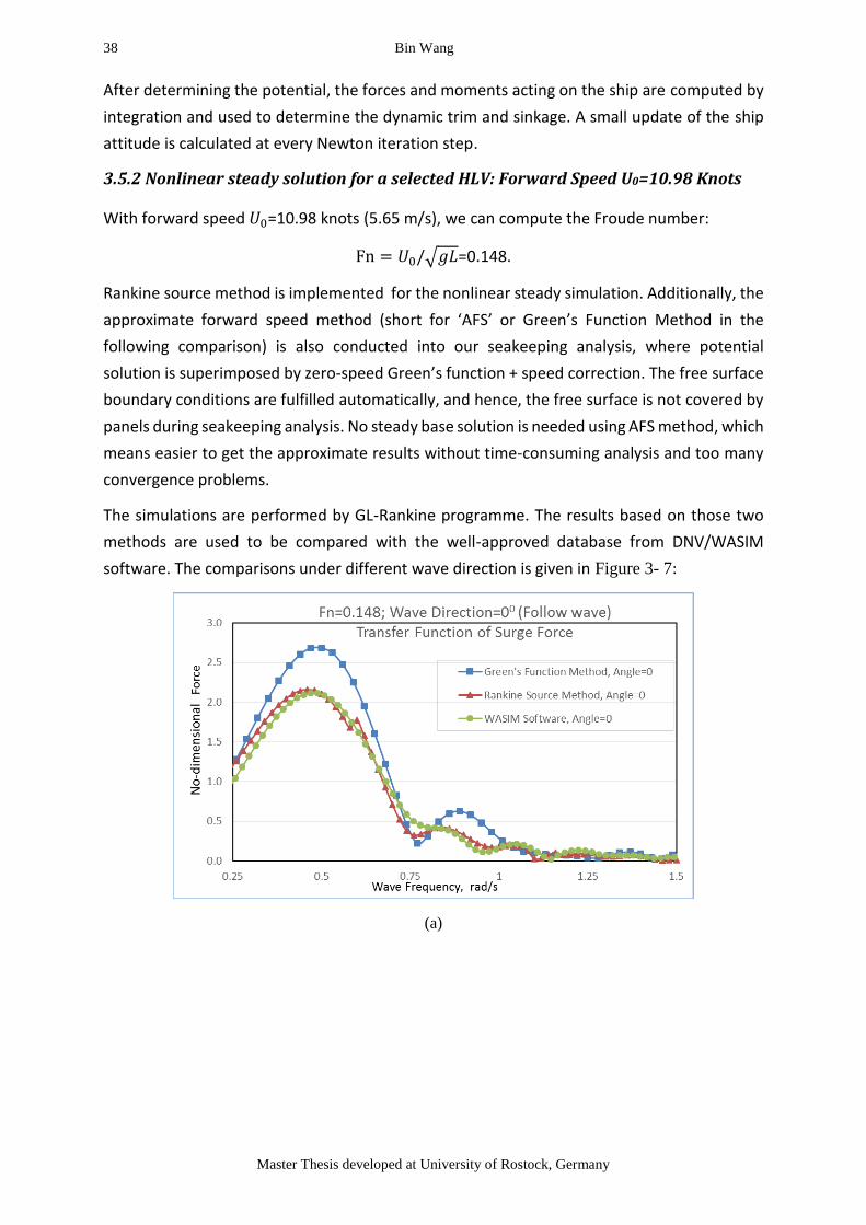
3.5.2 Nonlinear steady solution for a selected HLV: Forward Speed U0=10.98 Knots
With forward speed 𝑈0=10.98 knots (5.65 m/s), we can compute the Froude number:
Fn = 𝑈0/√𝑔𝐿=0.148.
Rankine source method is implemented for the nonlinear steady simulation. Additionally, the
approximate forward speed method (short for ‘AFS’ or Green’s Function Method in the
following comparison) is also conducted into our seakeeping analysis, where potential
solution is superimposed by zero-speed Green’s function + speed correction. The free surface
boundary conditions are fulfilled automatically, and hence, the free surface is not covered by
panels during seakeeping analysis. No steady base solution is needed using AFS method, which
means easier to get the approximate results without time-consuming analysis and too many
convergence problems.
The simulations are performed by GL-Rankine programme. The results based on those two
methods are used to be compared with the well-approved database from DNV/WASIM
software. The comparisons under different wave direction is given in Figure 3- 7:
(a)

Hydrodynamic Analysis of a Heavy Lift Vessel during Offshore Installation Operations 39
“EMSHIP” Erasmus Mundus Master Course, period of study September 2013 – February 2015
(b)
(c)
(d)

40 Bin Wang
Master Thesis developed at University of Rostock, Germany
(e)
(f)
Figure 3- 7 Force/Moment transfer functions for “Type I Vessel” in regular waves at 10.98 Knots.
From above comparisons, we can see that:
The results based on AFS method (zero-speed Green’s function + forward speed
correction) agree well with Rankine source method under most of conditions, which
approves that AFS method can be used as reference before more time-consuming
analysis to be performed.
It also reveals that some large deviations appear at certain wave frequencies and wave
directions. It is easy to understand that since the steady inflow is approximated as
parallel inflow in Green’s function method, which works well with a small forward
speed. Within high forward speed, the zero-speed Green function method delivers
low reliable results.

Hydrodynamic Analysis of a Heavy Lift Vessel during Offshore Installation Operations 41
“EMSHIP” Erasmus Mundus Master Course, period of study September 2013 – February 2015
Generally, the seakeeping analysis results from GL-Rankine show high-level
coincidence to WASIM’s, that both are based on Rankine source assumptions.
Beside of the possible modeling deviation, some existing small differences between
the two results may due to the different ways to obtain motions response. We already
know that in WASIM, the simulations are carried out in the time domain and then use
Fourier transformations to transfer the results if achievements are needed in
frequency domain, so during the process it can integrate time-dependent variables.
GL-Rankine only runs seakeeping analysis in frequency domain.
3.6 Seakeeping: 3-D Rankine sources V.S Frank’s 2-D strip pulsating
sources
Over the past years, several comparisons of strip theory predictions have been made with
model experimental data for head seas. Murdey[54] demonstrated the accuracy of predictions
through comparison with data from tests with the NRC hull form series for fast surface ships.
It concluded that, for Froude numbers below 0.5, early versions of strip theory models
predicted heave and pitch motions in regular waves to within 20% of the maximum measured
response. Karppinen[55] presented comparisons of strip theory predictions with model test
data for a wide-beam fishing vessel. Heave RAO's for both head and beam seas were predicted
to within 15% even at the relatively high Froude number of 0.8, with a lesser degree of
correlation for pitch RAO's.
In this section, we will compare the simulation results, one based on 3-D Rankine Source
method in GL-Rankine, another based on Frank’s 2-D strip method in Octopus.
3.6.1 Test model for numerical comparison
In Octopus, the following assumptions are introduced due to usage of the strip theory
approach:
- The pitch and yaw coefficients follow from the previous heave and sway coefficients
and the arm (i.e., the distance of the cross section to the center of gravity G).
- For each frequency, the two-dimensional potential hydrodynamic sway coefficient of
related equivalent longitudinal cross section is translated to two-dimensional potential
hydrodynamic surge coefficients by an empiric method.
- The 3-D coefficients follow from an integration of these 2-D coefficients over the ship’s
length[56].
The following table provides basic dimensions and characteristics of the selected ‘Type II’
vessel, which to be used in following numerical simulations. Again no trim or heel angle is set
at hydrostatic status and infinite water depth to be assumed.

42 Bin Wang
Master Thesis developed at University of Rostock, Germany
Table 3- 2 ‘Type II’ Vessel Parameters
TYPE Lpp /m Beam
/m
Depth
/m
Draft
/m
Displacement/
Mt
GMt
/m
Hull
Type II 123.9 23.0 11.4 7.8 16877 2.68
Accordingly, the two dimensional strip model as well as discretized 3-D panel model for vessel
hull are given in Figure 3- 8:
(a)
(b)
Figure 3- 8 Discrited hull models: 2-D strips (upper) V.S 3-D panels (lower)
3.6.2 Seakeeping using Frank’s method of pulsating source: Forward speed U0=8.5
knots
In 2-D strip seakeeping analysis, the pulsating source method of Frank is used. The theoretical
basis was already given, see sub-chapter 2.4.
With forward speed 𝑈0=8.5 knots (4.37 m/s), we can compute the Froude number:
Fn = 𝑈0/√𝑔𝐿=0.125.
One representative wave directions (α=400) condition is picked out and the corresponding
comparative results are given in six-degree of freedom, see following Figure 3- 9.

Hydrodynamic Analysis of a Heavy Lift Vessel during Offshore Installation Operations 43
“EMSHIP” Erasmus Mundus Master Course, period of study September 2013 – February 2015
(a)
(b)
(c)

44 Bin Wang
Master Thesis developed at University of Rostock, Germany
(d)
(e)
(f)
Figure 3- 9 Force/Moment transfer functions for “Type II Vessel” in regular waves at 8.5 Knots.

Hydrodynamic Analysis of a Heavy Lift Vessel during Offshore Installation Operations 45
“EMSHIP” Erasmus Mundus Master Course, period of study September 2013 – February 2015
From above comparisons, we can see that:
The results based on Frank’s method of pulsating source agree well with Rankine
source method under most of conditions, which corroborates that 2-D strip method
can be used to conduct a meaningful result before more time-consuming 3-D source
simulation to be performed.
It also reveals that some large deviations appear at certain wave frequencies and wave
directions. In general, the hydrodynamic forces from Octopus seem more
conservative. The possible reason is that 2-D strips integration method cannot catch too much
geometry changes along each axis direction, since uniform shape along each strip to
be assumed and only 3 degree of freedom to be considered at beginning.

46 Bin Wang
Master Thesis developed at University of Rostock, Germany
4. Cases Study in Frequency Domain: Hydrodynamic Interactions
between Two Ships
The frequent use of two or more closely positioned vessels during offshore operations makes
the study of multi-body systems an important topic. An important aspect of the thesis work is
to study hydrodynamic performance under such operation conditions.
This chapter focuses on multi-body analysis in regular waves in frequency domain. The purpose of
those investigations is to determine the hydrodynamic coefficients and exciting forces of the floating
body models that are close enough, i.e. heavy lift vessel (HLV) and transport barge during the cargo
transfer process.
Here we first introduce the theoretical basis of multi-body interaction in wave field. Then
these methods will be implemented in the following case studies to illustrate certain features
of the physical behavior.
4.1 Mathematic Solution for Two-body Hydrodynamic Problem
For the multiple body system, the number of the degrees of freedom of the mass matrix and
the body motion vector, is changed to 6N×6N, where N is the number of bodies. Here consider
two-body interaction case. Three sets of right-handed orthogonal coordinate systems are
used to describe the motions responses, as shown in Figure 4- 1.
O-XYZ is the space fixed coordinate system, OA-XAYAZA and OB-XBYBZB are the oscillatory
coordinate systems fixed with respect to ship A and B respectively. The O-XY plane coincides
with the undisturbed free surface. Oscillatory coordinate systems OA-XAYAZA and OB-XBYBZB will
be used to describe the body motion in six degrees of freedom with complex amplitudes ζ𝑖
(i=1,2,…, 12), where i=1,2,3,4,5,6 represents surge, sway, heave, roll, pitch and yaw motions
for ship A, and i=7,8,9,10,11,12 represent motions for ship B, respectively.
Figure 4- 1 Definition of Co-ordinate system[57]

Hydrodynamic Analysis of a Heavy Lift Vessel during Offshore Installation Operations 47
“EMSHIP” Erasmus Mundus Master Course, period of study September 2013 – February 2015
The hydrodynamic coefficients are solved in the following sequence[58]:
1. The radiation/diffraction problem for each body in isolation 2. The interaction problem resulting from radiation/scatter from body A in the presence
of body B, and radiation/scatter from body B in the presence of body A.
Where body A and B represent a pair of bodies which interact hydrodynamically. If there are
several bodies, the two-body problem should be addressed for each unique pair of bodies.
4.1.1 Theoretical Formulation
The total unsteady potential for a sinusoidal wave excitation with encounter frequency ωe,
can be expressed as:
ti
iiiDI
eezyxzyxtzyx
12
1
),,(),,(),,,( (4-1)
Where ФI (x,y,z) is the incident wave potential representing the incident waves; ФD (x,y,z) is
the diffraction potential representing the disturbance of the incident waves diffracted from
the body; Фi (i=1,2,… ,12) are the radiation potentials due to oscillations of the two bodies in
calm water with unit amplitude. The incident wave potential was given as follow
(4-2)
Where 𝜔0 is the wave frequency, ξa is the wave amplitude, k is the incident wave number
and k=ω02/g, β is an arbitrary heading angles (1800 for head sea).
The individual potentials have to satisfy in the fluid domain, on the free surface, the sea bed,
the submerged body surface and a suitable far-field radiation condition at infinity.
Laplace equation: 02 in the fluid domain (4-3)
Linear free surface condition: 02
zge
on z=0 (4-4)
Body boundary condition for diffraction potentials:
0)(
DI
n on ship A and ship B (4-5)
Body boundary condition for radiation potentials:
iei ni
n
(i=1, 2, ...6) on ship A (4-6)
(i=7, 8, ...12) on ship B (4-7)
(i=1, 2, ...6) on ship A (4-8)
(i=7, 8, ...12) on ship B (4-9)
Where,
tikykxikzaI
eeeeig
)sincos(
0
0
i
n
0
i
n
iei nin

48 Bin Wang
Master Thesis developed at University of Rostock, Germany
nnnn
),,( 321 on ship A; on ship A.
on ship B; on ship B.
Here n is the outward unit normal vector on ship A and ship B and r
is the position
vector with respect to the origin of the reference frame on ship A and ship B.
Sea bed condition: for z (4-10)
Radiation condition at infinity :
0)(lim
ik
nkr
kr at kr (4-11)
The wave exciting force 𝐹𝑖 can be divided into the incident wave part,𝐹𝑖𝐼, and the diffraction
part, 𝐹𝑖𝐷.
dsniFFF iSS
DIe
D
i
I
iiBA
)( (4-12)
The motion induced forces is
(4-13)
Where,
ijeijeij BiAT 2 (4-14)
The terms 𝐴𝑖𝑗 and 𝐵𝑖𝑗 are added mass and damping coefficients, respectively.
(4-15)
(4-16)
Under the assumption that the responses are linear and harmonic, the twelve linear coupled
differential equations of motion for two floating bodies can be written in the following form
for i=1,2...12 (4-17)
where, 𝑀𝑖𝑗 is the generalized mass matrix for the ship A and ship B, 𝐶𝑖𝑗is the restoring force
matrix for ship A and ship B, respectively. ζj is the complex amplitude of the response motion
in each of the six degree of freedom for each body, and Fi is the complex amplitude of the
wave exciting force for ship A and ship B.
4.1.2 Numerical Procedure
The diffraction potential and radiation potentials can be expressed in terms of well-known
Green functions, where by the distribution with the density on the surface SA and SB:
for P inside fluid (4-18)
The unknown source density can be found by imposing the body boundary conditions and it
gives:
nrnnn
),,( 654
nnnn
),,( 987 nrnnn
),,( 121110
0
n
12
1
12
1 j
jijiSS
j
j
jei TdsniEBA
dsnA iSS
j
e
ijBA
Im
dsnB iSS
jijBA
Re
12
1
2 ])([j
ijijijeijije FCBiAM
BA SSpQdsQPGQ )(4)(),()(

Hydrodynamic Analysis of a Heavy Lift Vessel during Offshore Installation Operations 49
“EMSHIP” Erasmus Mundus Master Course, period of study September 2013 – February 2015
for P on body surface (4-19)
where, Vn is the normal component of the velocity on the body surface.
For more detail about such procedure, see previous sub-chapter 2.2 or Telste and Noblesse’s
paper (1986).
4.1.3 Relative motion between two floating bodies
Finally, the longitudinal, horizontal and vertical relative motion between ship A and ship B at
any position can be expressed as three components,
)]()[(1
12117651
BBAA
aa
R yzyzL
(4-20)
(4-21)
(4-22)
where, (x𝐴, 𝑦𝐴, 𝑧𝐴) and (x𝐵 , 𝑦𝐵, 𝑧𝐵) are the coordinates of the position with respect to each
body frame system; see Figure 4- 1.
4.2 Verification Case: Two Freely Floating Cylinders in Finite Water
Depth
Based on above procedure, a numerical simulation consisting of two freely floating vertical
cylinders is performed in regular waves, under the purpose to study the interaction effects
and to justify the validity of the computer code. Again, the computing program GL-Rankine is
used to analyze this simple multi-body interaction problem.
The diameter and draft of each cylinder is 40.0 m and 10.0 m respectively. The separation
distance or, gap between them is 20.0 m. The water depth is considered as 200.0 m. The
wetted surface of each cylinder was divided into 1368 panels, as shown in Figure 4- 2. For 00
wave-heading angle, body I and body II represent the lee side and weather side cylinder
respectively.
(a)
BA SSnVQds
n
QPGQP )(
),()(
4
1)(
2
1
)]()[(1
10128462
BBAA
aa
R zxzxH
)]()[(1
10119453
BBAA
aa
R yxyxV

50 Bin Wang
Master Thesis developed at University of Rostock, Germany
(b)
Figure 4- 2 Mesh arrangements of the wetted surfaces of two floating vertical cylinders.
(a) Top view, (b) Side view
The numerical simulation results are plotted against 𝑘𝑎, where k and a denote the wave
number and radius of each cylinder respectively. The non-dimensional surge wave motions on
body I and body II are shown in Figure 4- 3, and Figure 4- 4 presents the heave motion
response of body I and body II.
Figure 4- 3 Surge motions of two vertical floating cylinders
Figure 4- 4 Heave motions of two vertical floating cylinders

Hydrodynamic Analysis of a Heavy Lift Vessel during Offshore Installation Operations 51
“EMSHIP” Erasmus Mundus Master Course, period of study September 2013 – February 2015
Figure 4- 3 and Figure 4- 4 also depict comparisons between the present simulation and
Matsui’s results [Matsui et al, 1981][59] [Mir T. A. and Yoshiyuki I. 2005] [60]. We can see the
high-level coincidence between both of them, which also approve that GL-Rankine software
to be capable for this case.
4.3 The Case to Study: hydrodynamic interaction in side-by-side
operation
According to the accommodation in marine operation guideline DNV-RP-C205[61] and DNV-RP-
H103[62], hydrodynamic interactions between multiple floaters in close proximity, or between
a floater and a large fixed structure in the vicinity of this floater, should be considered when
solving radiation/diffraction problems.
So an case of a two-body system consisting of a heavy lift vessel and a side-by-side positioned
transport barge during lifting operations (shown as Figure 4- 5) , will be studied here.
Figure 4- 5 A heavy lift vessel and a transport barge during cargo transfer operation : Topview (left)
& The gap (right). (Source of photoes: SAL Heavy Lift)
This is a typical situation happening during offshore engineering , where there may be strong
hydrodynamic interaction effects between the two floater. And the frequency- domain
analysis is performed with GL-Rankine software in freely floating condition, no motion
constraint between HLV and transport barge is considered.
4.3.1 Model Data
a. Vessel Model
Here ‘Type I’ heave lift vessel (HLV) is used again, but with one additional pontoon at starboard
side. The pontoon is connected with main hull via a relatively rigid steel frame. This box-
shaped pontoon can provide additional buoyance to improve the stability during the lifting
operations.
The principal dimensions of this ‘new’ HLV are listed in Table 4- 1.
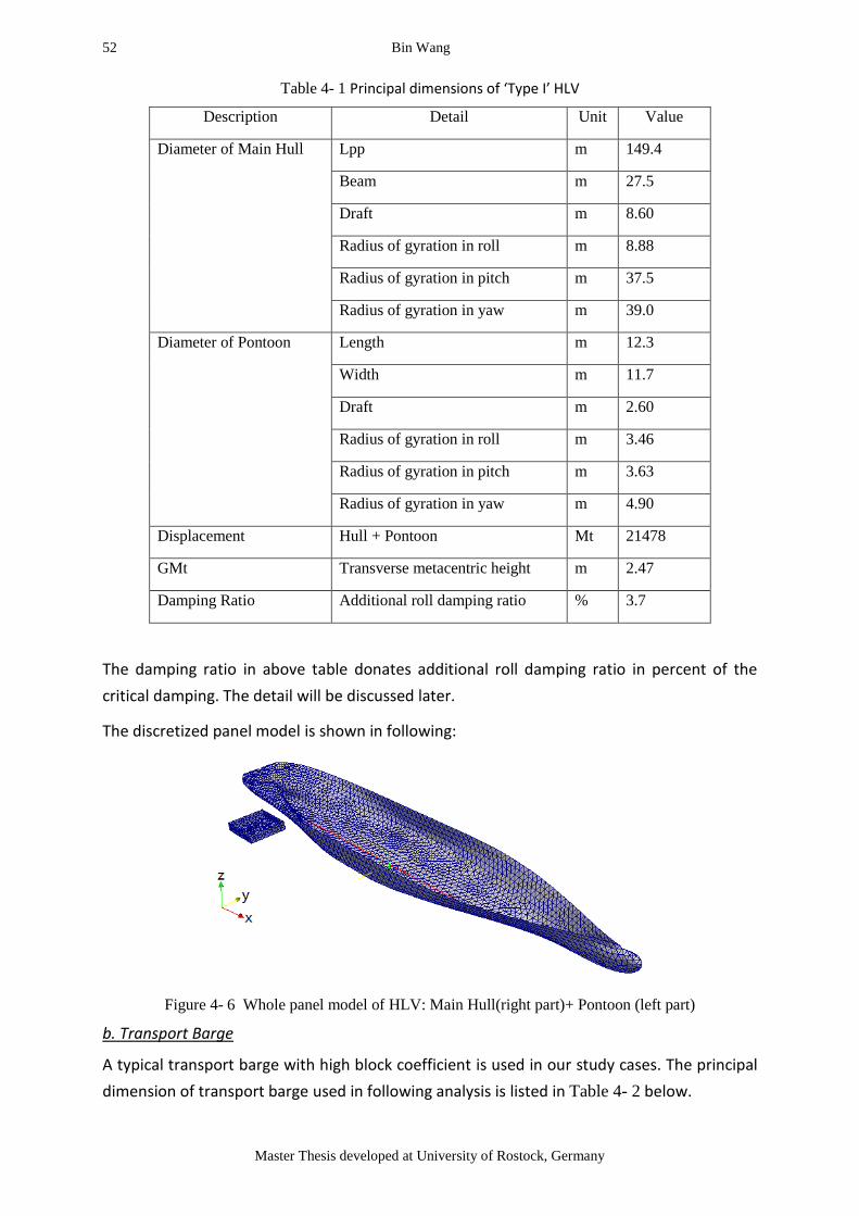
52 Bin Wang
Master Thesis developed at University of Rostock, Germany
Table 4- 1 Principal dimensions of ‘Type I’ HLV
Description Detail Unit Value
Diameter of Main Hull Lpp m 149.4
Beam m 27.5
Draft m 8.60
Radius of gyration in roll m 8.88
Radius of gyration in pitch m 37.5
Radius of gyration in yaw m 39.0
Diameter of Pontoon Length m 12.3
Width m 11.7
Draft m 2.60
Radius of gyration in roll m 3.46
Radius of gyration in pitch m 3.63
Radius of gyration in yaw m 4.90
Displacement Hull + Pontoon Mt 21478
GMt Transverse metacentric height m 2.47
Damping Ratio Additional roll damping ratio % 3.7
The damping ratio in above table donates additional roll damping ratio in percent of the
critical damping. The detail will be discussed later.
The discretized panel model is shown in following:
Figure 4- 6 Whole panel model of HLV: Main Hull(right part)+ Pontoon (left part)
b. Transport Barge
A typical transport barge with high block coefficient is used in our study cases. The principal
dimension of transport barge used in following analysis is listed in Table 4- 2 below.

Hydrodynamic Analysis of a Heavy Lift Vessel during Offshore Installation Operations 53
“EMSHIP” Erasmus Mundus Master Course, period of study September 2013 – February 2015
Table 4- 2 Principal dimensions of transport barge
Description Detail Unit Value
Diameter of Barge Lpp m 86.1
Beam m 27.5
Draft m 3.0
Radius of gyration in roll m 11.0
Radius of gyration in pitch m 24.1
Radius of gyration in yaw m 24.1
Displacement Mt 7204
GMt Transverse metacentric height m 19.23
Damping Ratio Additional roll damping ratio % 2.0
Accordingly, the discretized panel model of transport barge is shown as following:
Figure 4- 7 The panel models of transport barge
c. Coupled models and the gap
Though the transport barge to be positioned by tensioned winches and rubber fenders placed
between the gap during the cargo transfer process (as shown in Figure 4- 5), the motion
constraint or connecting stiffness’ are not considered here in frequency domain analysis, but
in time domain analysis in next chapter. Now is the free-free interaction case.
The gap (horizontal distance) between heave lift vessel and transport barge is set to be only
1.25 m, which may result strong resonance waves. This will be discussed later sub-chapter.
Finally, the panel models of two-body system consisting of a heavy lift vessel and a side-by-
side positioned transport barge, are shown as following:

54 Bin Wang
Master Thesis developed at University of Rostock, Germany
Figure 4- 8 Multi-body models (blue: HLV; green: Transport Barge) in GL-Rankine
d. Environmental Conditions
Similar as previous cases, wave heading is accounted anti-clockwise by the angle between x-
axis and wave propagation direction, see Figure 4- 9.
Figure 4- 9 Wave heading angle setting
Several typical wave directions (including 00, 450, 900, 3150) are conducted in analysis. Current
and wind is not considered in this study.
The water depth is set to be 20 meters only, which normally means the shallow water
conditions. Furthermore, the cargo transfer operation happened in open sea area, which
means no harbor or wall-shielding conditions were assumed here.
4.3.2 Multi-body analysis in regular waves in finite water depth
The added mass, added damping, exciting forces and moments are obtained in this frequency
domain analysis using GL-Rankine (short for ‘Rankine’ in the following). Main emphasis is put
on the hydrodynamic performance of the two vessels: how much their behavior changes from
the single body case to multi-body case.
Thus, there are two main steps to achieve that goal. First, single body analysis is performed in
order to obtain the response of HLV alone as well as of transport barge. Then, multi-body
analysis is carried out by placing HLV and the barge side-by-side, with 1.25 m horizontal

Hydrodynamic Analysis of a Heavy Lift Vessel during Offshore Installation Operations 55
“EMSHIP” Erasmus Mundus Master Course, period of study September 2013 – February 2015
distance. Based on the result from those two steps, the interaction effect can be observed, if
same environmental conditions to be used.
Figure 4- 10 Wave surface contours for a multi-body interaction case
a. Exciting Forces and Moments
It is convenient to show all the results here since a considerable amount of data and plots had
been generated during the case studies. Here gives the comparison of transfer function of
exciting forces for single-body and multi-body cases, under a representative wave direction.
(a) Surge RAO-Force
(b) Sway RAO-Force

56 Bin Wang
Master Thesis developed at University of Rostock, Germany
(c) Heave RAO-Force
(d) Roll RAO-Moment
(e) Pitch RAO-Moment
(f) Yaw RAO-Moment
Figure 4- 11 Transfer Functions of exciting forces & moments for single and multi-body cases in
limited water depth. (Left: Heave Lift Vessel; Right: Transport Barge)

Hydrodynamic Analysis of a Heavy Lift Vessel during Offshore Installation Operations 57
“EMSHIP” Erasmus Mundus Master Course, period of study September 2013 – February 2015
For this wave heading case, the results show that the existing of HLV on the weather side
provided an apparent “sheltering effect” which leads to smaller motions on the leeside
transport barge, as well as reducing forces in all six-degree of transport barge in relatively long
waves.
There are also some peak values appearing in high wave frequency zone during the multi-body
interaction analysis, especially for HLV, which looks unreasonable. This phenomena may due
to the trapped waves existing in the gap between structures and will be discussed later.
b. RAO of Average Drift Forces and Drift Moments
Beside of the wave frequency force, here is also interested to study the interaction influences
on mean drift forces, which is very important to dynamic positioning (DP) systems design or
mooring design during the offshore operations.
Based on the potentials, which were solved by zero-speed Green function method, the first-
order pressure is computed, and then quadratic transfer functions (i.e., forces and moments
proportional to wave amplitude squared) are computed to obtain side drift forces in waves.
As we can image, when calculating individual drift forces on multiple floaters, direct pressure
integration of second order fluid pressure on each body to be conducted, which is well known
as “Near-field Method”. Wave heading= 315 degree case is picked for instance and here lists
three components in one set of six-degree mean drift forces/moments.
(a) (b)
(c)
Figure 4- 12 HLV Mean Drift Forces in 3150 incoming waves. Selected: (a) Sway; (b) Heave; (c)
Yaw

58 Bin Wang
Master Thesis developed at University of Rostock, Germany
Figure 4- 12 shows that the interaction effect may produce both positive and negative mean
drift forces. The negative mean drift force may be produced from the reflection wave due to
the presence of Transport Barge.
Further, in the radiation problem, the presence of the hydrodynamic interaction between HLV
and Barge can be revealed from the added mass and potential damping coefficients. Both
added mass and potential damping are frequency dependent. Due to space limits, those
results will not be listed here.
4.4 Some Notes & Discussions
4.4.1 Additional roll damping ratio
As mentioned in model data (see Table 4- 1 and Table 4- 2), Blume’s method [63] is used to
characterize roll damping in the program. The method defines effective linear viscous
damping term 𝐵𝑣 , based on the application of a time-harmonic exciting roll moment 𝑀 of
known frequency and amplitude, to account for the strong non-linearity of the damping force,
especially in the roll motion.
The coefficient of the equivalent linear roll damping can be obtained from:
𝑏𝑒𝑓𝑓 =𝑀
𝜑𝑟𝑒𝑠√𝐼𝜑𝑐𝜑⁄ (4-23)
where
𝑀 is the static moment
𝐼𝜑 is the moment of inertia with respect to the roll axis (including added moment of inertia).
𝜑𝑟𝑒𝑠 is the corresponding resonance roll amplitude at the resonance frequency 𝜔𝜑
𝜔𝜑 = √𝑐𝜑/𝐼𝜑 , where 𝑐𝜑 = 𝑚𝑔𝐺𝑀𝑡 is the stiffness coefficient and 𝑚 is the mass
displacement.
For more detail, please see [Ould el M.and Vladimir S. et.][64]
4.4.2 Asymmetric Structures
As stated in sub-chapter 4.3.1, the HLV is comprised by main hull and additional pontoon,
which means an asymmetric structures.
Beside of adjusted metacentric height and shifted CoG, the combining of inertia moments
results in six new products: I𝑥𝑦 = I𝑦𝑥 , I𝑥𝑧 = I𝑧𝑥 and I𝑦𝑧 = I𝑧𝑦 , called products of inertia,
which normally be zero for symmetric vessels. Then those products listed in mass/inertia
matrix 𝑀 are involved in solving of the hydro-mechanical problem 𝑀𝑋 " = ∑𝐹 𝑒𝑥𝑡, and finally
resulted significant influence on the ship motions.

Hydrodynamic Analysis of a Heavy Lift Vessel during Offshore Installation Operations 59
“EMSHIP” Erasmus Mundus Master Course, period of study September 2013 – February 2015
4.4.3 Irregular Frequencies.
Beside of resonant response with damped natural frequencies of structures, irregular
frequencies may occur in a narrow bandwidth always causing unwanted numerical problems.
As stated before, if the Green theorem is applied, the velocity potential turns out to be a
solution of the Fredholm integral equation of second kind[65]:
α∅(x) + ∫ ∅(𝜉)𝜕𝐺(𝑥; 𝜉)
𝜕𝑛𝑑𝑆 = ∫
𝜕∅(𝜉)
𝜕𝑛𝐺(𝑥; 𝜉)𝑑𝑆
𝑆𝑆
(4-24)
where n is the unit normal vector on the body surface pointing toward fluid, α is the solid
angle, and 𝑆 is the boundary surface. 𝐺(𝑥; 𝜉) is the wave Green function according to
[Wehausen and Laitone, 1960], see sub-chapter 2.2.2.
The above integral equation may not have a unique solution at specific frequencies, which are
called irregular frequencies. This is related with an internal resonance. Irregular frequencies
may occur at high encounter frequencies. A typical indication for an irregular frequency is a
large condition number of the equation system or very ‘noisy’ transfer functions.
Irregular frequencies correspond to standing waves inside the body. To eliminate irregular
frequencies, an internal boundary inside the body was generated (source distribution) in GL-
Rankine during simulations.
4.4.4 Resonance Trapped Waves
If we look carefully at the transfer functions results (see Figure 4- 11) from multi-body analysis,
some peak values seem far beyond the data from single body analysis. This important
interaction effect may due to a near resonance trapped wave between the floaters which can
excite sway and roll motions. This trapped wave is undamped within potential theory.
Additional resonance peaks also appear in coupled heave, pitch and roll motions.
According to DNV guidelines, hydrodynamic resonance may occur in the gap between the two
vessels that are situated closely side-by-side. There are three types of resonant motions to be
considered:
- Piston mode motion, where the volume of water between the vessels heaves up and down more or less like a rigid body. This mode of motion is also called the pumping or Helmholtz mode.
- Longitudinal sloshing mode, where the water between the vessels moves back and forth in the longitudinal direction.
- Transverse sloshing mode, where the water motion between the vessels is a standing wave between the vessels with a wavelength on the order of the gap width.
The eigenfrequencies 𝜔𝑛 corresponding to the hydrodynamic resonances in the gap can be
conducted from[66]:

60 Bin Wang
Master Thesis developed at University of Rostock, Germany
𝜔𝑛2 = 𝑔𝜆𝑛
1 + 𝐽𝑛0 tanh 𝜆𝑛𝑑
𝐽𝑛0+ tanh 𝜆𝑛𝑑 (4-25)
where
𝐽𝑛0(𝑟) =2
𝑛𝜋2𝑟∫
𝑟2
𝑢2√𝑢2 + 𝑟2
1
0
[1 + 2𝑢 + (𝑢 − 1) cos(𝑛𝜋𝑢)
−3
𝑛𝜋sin(𝑛𝜋𝑢)] 𝑑𝑢 −
1
𝑠𝑖𝑛𝜃0+ 1 + 2𝑟 𝑙𝑛
1 + 𝑐𝑜𝑠𝜃01 − 𝑐𝑜𝑠𝜃0
(4-26)
𝑟 = 𝑏/𝑙
𝑏 = 𝑤𝑖𝑑𝑡ℎ 𝑜𝑓 𝑡ℎ𝑒 𝑔𝑎𝑝 𝑏𝑒𝑡𝑤𝑒𝑒𝑛 𝑣𝑒𝑠𝑠𝑒𝑙𝑠 [𝑚]
𝑙 = 𝑙𝑒𝑛𝑔𝑡ℎ 𝑜𝑓 𝑡ℎ𝑒 𝑔𝑎𝑝 (𝑎𝑝𝑝𝑟𝑜𝑥𝑖𝑚𝑎𝑡𝑒𝑑 𝑏𝑦 𝑙𝑒𝑛𝑔𝑡ℎ 𝑜𝑓 𝑠ℎ𝑜𝑟𝑡𝑒𝑠𝑡 𝑣𝑒𝑠𝑠𝑒𝑙) [𝑚]
𝑑 = 𝑑𝑟𝑎𝑓𝑡 𝑜𝑓 𝑣𝑒𝑠𝑠𝑒𝑙𝑠 (𝑎𝑠𝑠𝑢𝑚𝑒𝑑 𝑡𝑜 ℎ𝑎𝑣𝑒 𝑠𝑖𝑚𝑖𝑙𝑎𝑟 𝑑𝑟𝑎𝑓𝑡) [𝑚]
𝑔 = 𝑎𝑐𝑐𝑒𝑙𝑒𝑟𝑎𝑡𝑖𝑜𝑛 𝑜𝑓 𝑔𝑟𝑎𝑣𝑖𝑡𝑦 [𝑚/𝑠2]
𝜆𝑛 = 𝑛𝜋/𝑙 [𝑚−1]
𝜃0 = 𝑡𝑎𝑛−1(1/𝑟) [𝑟𝑎𝑑]
The function 𝐽𝑛 versus 𝑛𝜋𝑟 is shown in Figure 4- 13. The eigenfrequency of the piston mode
is obtained by setting 𝑛 = 1 while The eigenfrequencies of sloshing modes are obtained by
setting 𝑛 = 2,3,4…. in above general expression.
Figure 4- 13 Function 𝐽𝑛 versus 𝑛𝜋𝑟 for piston mode (n=1, solid line) and lowest sloshing mode
(n=2, dotted line) (Source :DNV-GL)
A simplified expression for the eigenfrequency of the piston mode is also given by[67]:
𝜔12 =
𝑔
𝑑 +𝑏𝜋 (1.5 + 𝑙𝑛
𝐵2𝑏) (4-27)
where 𝐵 is the total beam of the two vessels including the gap between the vessels.
For our studied case, where vessels are located in close proximity with a narrow gap, the
eigenfrequencies of transverse sloshing are high and may be neglected. Only piston mode and
longitudinal sloshing mode are valuable to us.
Here the resonant piston mode in the narrow gap between main hull of HLV and the transport
barge is picked out for consideration, which may be the cardinal situation in our studied case.
Based on above equations, we can conduct the eigenfrequency ω𝑛1 = 1.46 𝑟𝑎𝑑 /s or
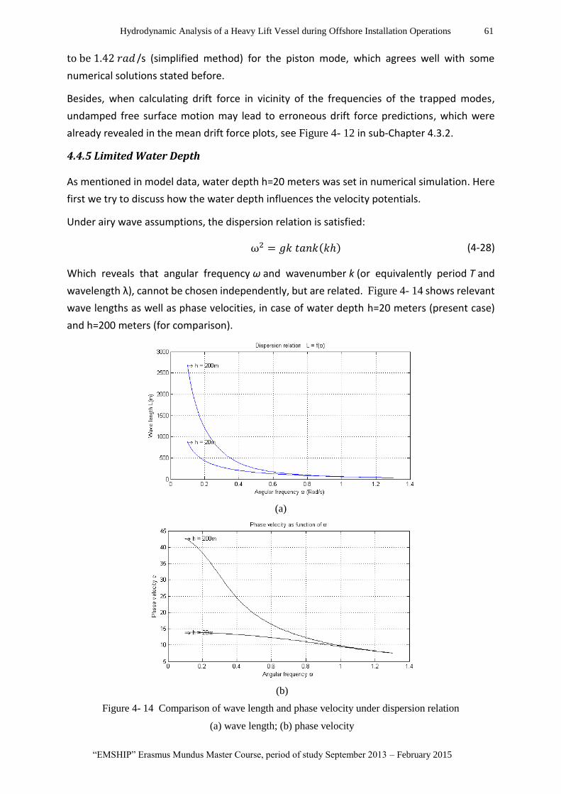
Hydrodynamic Analysis of a Heavy Lift Vessel during Offshore Installation Operations 61
“EMSHIP” Erasmus Mundus Master Course, period of study September 2013 – February 2015
to be 1.42 𝑟𝑎𝑑 /s (simplified method) for the piston mode, which agrees well with some
numerical solutions stated before.
Besides, when calculating drift force in vicinity of the frequencies of the trapped modes,
undamped free surface motion may lead to erroneous drift force predictions, which were
already revealed in the mean drift force plots, see Figure 4- 12 in sub-Chapter 4.3.2.
4.4.5 Limited Water Depth
As mentioned in model data, water depth h=20 meters was set in numerical simulation. Here
first we try to discuss how the water depth influences the velocity potentials.
Under airy wave assumptions, the dispersion relation is satisfied:
ω2 = 𝑔𝑘 𝑡𝑎𝑛𝑘(𝑘ℎ) (4-28)
Which reveals that angular frequency ω and wavenumber k (or equivalently period T and
wavelength λ), cannot be chosen independently, but are related. Figure 4- 14 shows relevant
wave lengths as well as phase velocities, in case of water depth h=20 meters (present case)
and h=200 meters (for comparison).
(a)
(b)
Figure 4- 14 Comparison of wave length and phase velocity under dispersion relation
(a) wave length; (b) phase velocity

62 Bin Wang
Master Thesis developed at University of Rostock, Germany
From above comparison, we can clearly see that for wave frequency less than 1.0 rad/s,
current water depth (h=20 m) has significantly changed wave length and phase velocity, which
means ‘shallow water’ situation.
Further, the water pressure distribution under ‘shallow water’ and deeper water is also quite
different. For comparison purpose, wave frequency ω=0.5 rad/s is selected within different
water depth and the dynamic wave pressure fields are computed accordingly, using airy wave
theory, see Figure 4- 15.
(a)
(b)
Figure 4- 15 Wave Pressure Distribution along position Z= 0~20 m under different water depths.
(a) Water Depth h=20 m (present case); (b) Water Depth h=200 m
The influence from water depth will be reflected to the diffraction/radiation potential solution
and finally to the ship motions. The following Figure 4- 16 gives the comparison of motion

Hydrodynamic Analysis of a Heavy Lift Vessel during Offshore Installation Operations 63
“EMSHIP” Erasmus Mundus Master Course, period of study September 2013 – February 2015
RAOs under two different water depth: ℎ𝑠ℎ𝑎𝑙𝑙𝑜𝑤 = 20 𝑚 (present case) and : ℎ𝐷𝑒𝑒𝑝 =
1000 𝑚 (for comparison).
(a)
(b)
(c)
Figure 4- 16 Ship motions under different water depths, Incoming wave angle=0 degree
(a) Surge motion; (b) Heave motion; (c) Roll motion
From above comparisons, we can see the motion characteristics show large deviations, after
reducing the water depth. The horizontal shifting increased while the vertical motion
decreasing.
Generally, those differences become significant only in low wave frequency zone, where
presents the trend that dispersion parameter μ = (wave number ∗ water depth) ≪ O(1),
and non-linear parameter ϵ =wave amplitude
water depth≫ 𝑂(0). Under shallow water scale conditions,
whether the dispersion relation (which was the basis of the wave model used in above analysis)

64 Bin Wang
Master Thesis developed at University of Rostock, Germany
works well or not become an issue, but this topic is not in this paper’s discussion range. For
details, please read relevant hydrodynamic books.
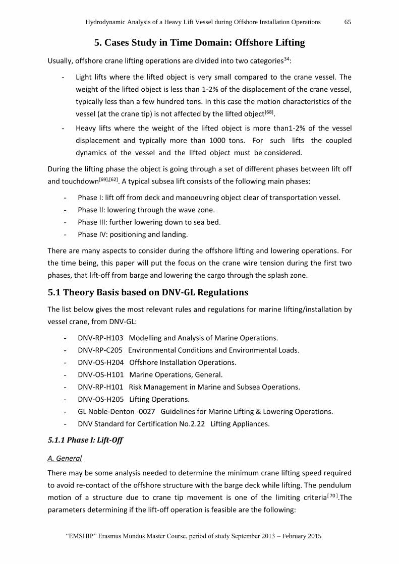
Hydrodynamic Analysis of a Heavy Lift Vessel during Offshore Installation Operations 65
“EMSHIP” Erasmus Mundus Master Course, period of study September 2013 – February 2015
5. Cases Study in Time Domain: Offshore Lifting
Usually, offshore crane lifting operations are divided into two categories34:
- Light lifts where the lifted object is very small compared to the crane vessel. The
weight of the lifted object is less than 1-2% of the displacement of the crane vessel,
typically less than a few hundred tons. In this case the motion characteristics of the
vessel (at the crane tip) is not affected by the lifted object[68].
- Heavy lifts where the weight of the lifted object is more than1-2% of the vessel
displacement and typically more than 1000 tons. For such lifts the coupled
dynamics of the vessel and the lifted object must be considered.
During the lifting phase the object is going through a set of different phases between lift off
and touchdown[69],[62]. A typical subsea lift consists of the following main phases:
- Phase I: lift off from deck and manoeuvring object clear of transportation vessel.
- Phase II: lowering through the wave zone.
- Phase III: further lowering down to sea bed.
- Phase IV: positioning and landing.
There are many aspects to consider during the offshore lifting and lowering operations. For
the time being, this paper will put the focus on the crane wire tension during the first two
phases, that lift-off from barge and lowering the cargo through the splash zone.
5.1 Theory Basis based on DNV-GL Regulations
The list below gives the most relevant rules and regulations for marine lifting/installation by
vessel crane, from DNV-GL:
- DNV-RP-H103 Modelling and Analysis of Marine Operations.
- DNV-RP-C205 Environmental Conditions and Environmental Loads.
- DNV-OS-H204 Offshore Installation Operations.
- DNV-OS-H101 Marine Operations, General.
- DNV-RP-H101 Risk Management in Marine and Subsea Operations.
- DNV-OS-H205 Lifting Operations.
- GL Noble-Denton -0027 Guidelines for Marine Lifting & Lowering Operations.
- DNV Standard for Certification No.2.22 Lifting Appliances.
5.1.1 Phase I: Lift-Off
A. General
There may be some analysis needed to determine the minimum crane lifting speed required
to avoid re-contact of the offshore structure with the barge deck while lifting. The pendulum
motion of a structure due to crane tip movement is one of the limiting criteria[ 70 ].The
parameters determining if the lift-off operation is feasible are the following:

66 Bin Wang
Master Thesis developed at University of Rostock, Germany
- The hoisting speed of the crane (depends on the weight of the object to be lifted).
- The combined motion characteristics of the barge and the crane vessel.
- The weather condition, combined with the orientation of the two vessels.
When lifting an object from the barge by means of a crane on board a crane vessel positioned
side by side with the barge, a critical parameter is the relative motion between the crane hook
and the barge at the position of the lifted object. The statistics of the relative motion
determines the probability that the barge will hit the lifted object after lift-off.
Once the object is lifted free of the transport barge, the object will be hanging from the crane,
and is being subject to the motion of the crane top. Since the length of the wire is short in this
case, the dynamic response of the object/wire system will be marginal, and the force in the
wire can be estimated from the vertical acceleration of the crane top alone.
For operations involving multiple cranes the maximum out of plumb of hoist lines should be
defined/calculated and considered in the calculations[71].
B. Probability of barge hitting lifted object[62]
A criterion for characterization of the safety of the lifting operation is that the object is not re-
hit by the barge after having been lifted off. The safety of the operation can be assessed by
estimating the probability that the lifted object will be hit by the barge and ensuring that the
probability is less than a certain prescribed value.
The following simplifying assumptions are made for the statistical analysis:
- The motion responses of the two vessels are assumed to be narrow banded.
- The hoisting speed U is constant during lifting.
- The lifted object is leaving the barge as the relative vertical motion a between the
barge and the crane hook has a maximum.
- The probability that the lifted object will be hit by the barge more than once
is practically zero. Consequently only the first possible hit is considered.
The probability P that the lifted object will be hit by the barge at the next maximum value of
the relative motion can be approximated by:
))2
()4
exp(2
1)(2
exp(2
1)(
22 erfcP (5-1)
Where:
τ =U 𝑇𝑧π
σ, 𝑒𝑟𝑓𝑐(𝑥) =
2
√𝜋∫ 𝑒−𝑡
2∞
𝑥dt (5-2)
U = hoisting speed [m/s]
Tz = zero up-crossing period for relative motion [s]
σ = standard deviation of relative motion [m]
The probability P is plotted in Figure 5- 1.

Hydrodynamic Analysis of a Heavy Lift Vessel during Offshore Installation Operations 67
“EMSHIP” Erasmus Mundus Master Course, period of study September 2013 – February 2015
Figure 5- 1 Probability of barge hitting lifted object. (Source : DNV-RP-H103)
Requiring the probability to be less than a given number ε, gives implicitly a value for the
maximum standard deviationσof the relative motion which is proportional to the significant
wave height 𝐻𝑠.
5.1.2 Phase II: Through splash zone
A. General
The “through the splash zone” phase starts when the cargo is lowered down and the bottom
end of the cargo begins submerging into the water. An object lowered into or lifted out of
water will be exposed to a number of different forces acting on the cargo. In general the
following forces should be taken into account when assessing the response of the object;
• 𝐹𝑙𝑖𝑛𝑒 = force in hoisting line/cable
• 𝑊0 = weight of object (in air)
• 𝐹𝐵 = buoyancy force
• 𝐹𝐶 = steady force due to current
• 𝐹𝐼 = inertia force
• 𝐹𝑤𝑑 = wave damping force
• 𝐹𝑑 = drag force
• 𝐹𝑤 = wave excitation force
• 𝐹𝑠 = slamming force
• 𝐹𝑒 = water exit force
The motions of the installation vessel combined with the motion of surface waves will create
a significant load on the object when it is lowered through the splash zone. It is important to
determine the wave loads during the passage through the splash zone and the added mass
and damping when the object is submerged to the seabed. However, the added mass and drag
coefficients are immersion dependent. The installed structure should be exposed to extreme
direct wave loading in the analysis. The added mass associated with the installed structure at
different submerged volumes may be estimated using the radiation/diffraction software.

68 Bin Wang
Master Thesis developed at University of Rostock, Germany
B. Hydrodynamic Forces on The Object: Simplified Method in DNV Rules
The Simplified Method supersedes the recommendations for determination of
environmental load effects given in DNV Rules for Marine Operations. The Simplified Method
is based upon the following main assumptions[72]:
- The horizontal extent of the lifted object (in the wave propagation direction) is
relatively small compared to the wave length.
- The vertical motion of the object follows the crane tip motion.
- The load case is dominated by the vertical relative motion between object and water,
which means other modes of motions can be disregarded.
Heave, pitch and roll RAOs for the vessel should be combined with crane tip position to find
the vertical motion of the crane tip.
An object lowered into or lifted out of water will be exposed to a number of different forces
acting on the structure. Beside of static weight of the submerged object, the following
hydrodynamic forces or parameters should be taken into account when assessing the
response of the object in general case:
I). Slamming impact force
Slamming forces are short-term impulse forces that acts when the structure hits the water
surface:
(5-3)
𝐴𝑠 is the relevant slamming area on the exposed structure part. 𝐶𝑠 is slamming coefficient.
The slamming velocity 𝑣𝑠, is :
22
wctcs vvvv (5-4)
Where,
𝑣𝑐 = lowering speed
𝑣𝑐𝑡 = vertical crane tip velocity
𝑣𝑤 = vertical water particle velocity at water surface
II). Varying buoyancy force
Varying buoyancy 𝐹𝜌, is the change in buoyancy due to the water surface elevation.
(5-5)
δV is the change in volume of displaced water from still water surface to wave crest or
wave trough.
δV = 𝑤 ∙ √ζ𝑎
2+ η𝑐𝑡
2 (5-6)
Where:
25.0 sssslam vACF
gVF

Hydrodynamic Analysis of a Heavy Lift Vessel during Offshore Installation Operations 69
“EMSHIP” Erasmus Mundus Master Course, period of study September 2013 – February 2015
ζ𝑎
= wave amplitude
η𝑐𝑡= crane tip motion amplitude
𝑤= mean water line area in the wave surface zone
III). Drag force
Drag forces are flow resistance on submerged part of the structure. The drag forces are
related to relative velocity between object and water particles. There are two sources:
a. Friction force: Due to viscosity of the water and roughness of the objects surface a
velocity dependent friction force is generated. The friction force will always work in
opposite direction of the movement.
b. Wake: The water flow creates wakes around corners, the wakes creates an area with
lower pressure. This creates a force opposite of the direction of the movement
The drag coefficient, C𝐷, in oscillatory flow for complex subsea structures may typically be
C𝐷≥2.5.
(5-7)
Relative velocity, 𝑣𝑟, is found by:
(5-8)
Where,
𝑣𝑐 = lowering/hoisting speed.
𝑣𝑐𝑡 = vertical crane tip velocity.
𝑣𝑤 = vertical water particle velocity at water depth, d.
𝐴𝑝 = horizontal projected area.
IV). Mass force
“Mass force” is here a combination of inertia force, Froude-K force and diffraction force.
The overview of mass forces is as Figure 5- 2. All of this mass must be accelerated when
the crane tip acceleration is transferred to the load.
Figure 5- 2 Mass force on the object. (Source: Arnstein Hosaas, Subsea 7)
25.0 rPDD vACF
22
wctcr vvvv

70 Bin Wang
Master Thesis developed at University of Rostock, Germany
Crane tip acceleration and water particle acceleration are assumed statistically
independent, then mass force 𝐹𝑀:
(5-9)
Where,
𝑀 = mass of object in air
𝐴33 = heave added mass of object
𝑎𝑐𝑡 = vertical crane tip acceleration
𝑉 = volume of displaced water relative to the still water level
𝑎𝑤 = vertical water particle acceleration at water depth, d.
About added mass 𝐴33:
- Hydrodynamic added mass for flat plates: depends on body shape.
- Added mass increase due to body height.
- A volume of water partly enclosed within large plated surfaces will also contribute to
the added mass.
- No reduction applied in added mass when perforation is small.
V). Total Hydrodynamic Forces:
During lowering through the water surface, the structure may have both fully submerged
parts and items in the splash zone. The slamming force acting on the surface crossing item
is then in phase with the drag force acting on the fully submerged part. Likewise, the mass
and varying buoyancy forces are 1800 out of phase.
The characteristic hydrodynamic force is a time dependent function of slamming impact
force, varying buoyancy, hydrodynamic mass forces and drag forces. In the Simplified
Method the forces may be combined as follows:
(5-10)
where
𝐹𝐷 = characteristic hydrodynamic drag force.
𝐹𝑠𝑙𝑎𝑚 = characteristic slamming impact force.
𝐹𝑀 = characteristic hydrodynamic mass force.
𝐹𝜌 = characteristic varying buoyancy force.
Water particle velocity and acceleration are related to the vertical center of gravity for
each main item. Mass and drag forces contributions are then summarized:
i
MiM FF and (5-11)
𝐹𝑀𝑖 and 𝐹𝐷𝑖 are the individual force contributions from each main item.
2
33
2
33 ])[(])[( wctM aAVaAMF
22 )()( FFFFF MslamDhyd
][NFFi
DiD

Hydrodynamic Analysis of a Heavy Lift Vessel during Offshore Installation Operations 71
“EMSHIP” Erasmus Mundus Master Course, period of study September 2013 – February 2015
The static and hydrodynamic force should be calculated for different stages. The structure
may be divided into main items and surfaces contributing to the hydrodynamic force.
VI). Summary of simplified method.
The intention of the Simplified Method is to give simple conservative estimates of the
forces acting on the object. Pay attention that the Simplified Method is not applicable if
the crane tip oscillation period or the wave period is close to the resonance period 𝑇𝑛 , of
the hoisting system.
Also pay attention to the assumption that the horizontal extent of lifted object is relatively
small compared to the wave length, and if 𝐷 > 0.5𝜆 (where D is the horizontal dimension,
λ is the wave length), this simplified method will not applicable anymore.
The Simplified Method provides an excellent and efficient basis for lifting analysis, based
on the feedback from projects (K. Aarset 2011) [73].
5.2 Lift-off Simulations
During the lifting operation the lifted structure will be affected by the irregular motion of the
waves and the vertical motion of the crane tip as a result of the vessel motion. It is a quite
complex & time dependent system, even after the reduction in degrees of freedom, this is a
highly complex system and should hence be analyzed by a numerical computer program if
more accurate solution needed, such as Orcaflex software from Orcina.
5.2.1 Software: Orcaflex
Orcaflex is a non-linear time domain finite element program which is frequently used within
the offshore industry due to its graphical and easy-to-use interface. OrcaFlex has a very wide
range of applications in marine engineering and offshore renewable energy industry. WithIn
the domain of installation analysis, the program has the capabilities to analyze a number of
marine operations such as[74]:
• Pipelay analysis
• Anchor and mooring deployment
• Riser installation
• Cable lay dynamics
• Through-splash zone deployment
• Deep water installation of subsea hardware
• Seabed plough deployment and operation
• Offshore lift dynamics
• Deflect-to-connect and cross-seabed pull-in
• Stab and Hinge simulation
The vessel model can be endowed with correct hydrodynamic characteristic by importing
response data from diffraction/radiation programs. The hydrodynamic forces on line elements

72 Bin Wang
Master Thesis developed at University of Rostock, Germany
are calculated based on an extended version of the Morison equation and cross flow
assumptions. Orcaflex also uses “lumped mass” elements and “6D-bouys”, to simulate
structural elements such as beams, pipes and plates. The elements will simplify the
mathematical formulation and reduce the overall computational time.
5.2.2 Model data
a. Ship models and lifting object
Again, the ‘type I’ heave lift vessel as well as transport barge are introduced during the cargo
transfer (lift-off) operation, see Figure 5- 3(a)&(b). Their principal dimensions can be found
in previous chapter. Multi-body hydrodynamic analysis results in frequency domain are
imported, so that time-domain simulations for lift-off operations can be performed including
the interaction effects.
Additionally, bi-linear springs acting in surge and sway movement are modelled to work as
motion constraint in horizontal direction, to simulate the fenders and winch connection
between HLV and transport barge in the real world.
(a) (b)
(c)
Figure 5- 3 Models in Orcaflex. (Upper: the whole model in simulation; Bottom: lifted object)
The object to lift is a simplified box-shaped manifold, which is placed on the centre of barge
deck in initial condition. The weight of this manifold is 220 MT in air, with a main dimension
of L × B × H =6.70×5.50×3.72 meter. Four slings are used during the lifting simulation,
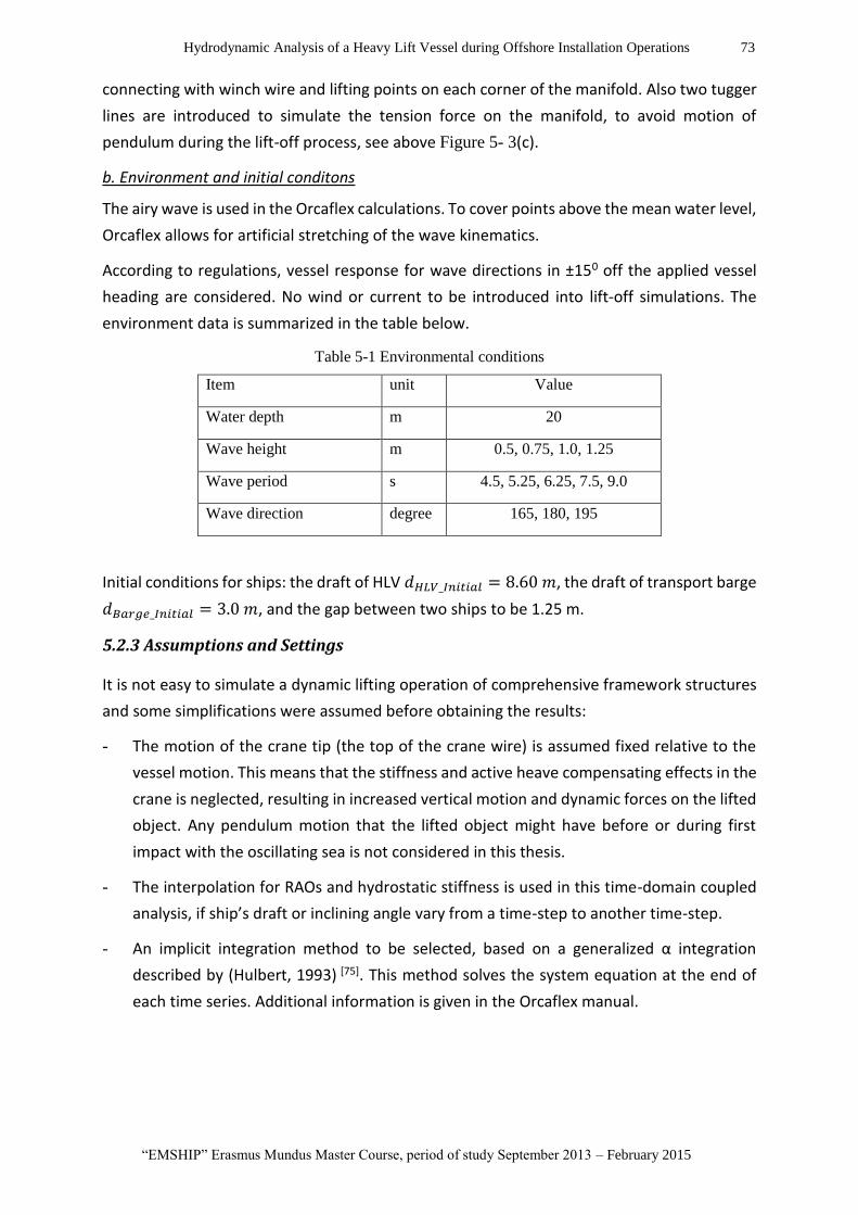
Hydrodynamic Analysis of a Heavy Lift Vessel during Offshore Installation Operations 73
“EMSHIP” Erasmus Mundus Master Course, period of study September 2013 – February 2015
connecting with winch wire and lifting points on each corner of the manifold. Also two tugger
lines are introduced to simulate the tension force on the manifold, to avoid motion of
pendulum during the lift-off process, see above Figure 5- 3(c).
b. Environment and initial conditons
The airy wave is used in the Orcaflex calculations. To cover points above the mean water level,
Orcaflex allows for artificial stretching of the wave kinematics.
According to regulations, vessel response for wave directions in ±150 off the applied vessel
heading are considered. No wind or current to be introduced into lift-off simulations. The
environment data is summarized in the table below.
Table 5-1 Environmental conditions
Item unit Value
Water depth m 20
Wave height m 0.5, 0.75, 1.0, 1.25
Wave period s 4.5, 5.25, 6.25, 7.5, 9.0
Wave direction degree 165, 180, 195
Initial conditions for ships: the draft of HLV 𝑑𝐻𝐿𝑉_𝐼𝑛𝑖𝑡𝑖𝑎𝑙 = 8.60 𝑚, the draft of transport barge
𝑑𝐵𝑎𝑟𝑔𝑒_𝐼𝑛𝑖𝑡𝑖𝑎𝑙 = 3.0 𝑚, and the gap between two ships to be 1.25 m.
5.2.3 Assumptions and Settings
It is not easy to simulate a dynamic lifting operation of comprehensive framework structures
and some simplifications were assumed before obtaining the results:
- The motion of the crane tip (the top of the crane wire) is assumed fixed relative to the
vessel motion. This means that the stiffness and active heave compensating effects in the
crane is neglected, resulting in increased vertical motion and dynamic forces on the lifted
object. Any pendulum motion that the lifted object might have before or during first
impact with the oscillating sea is not considered in this thesis.
- The interpolation for RAOs and hydrostatic stiffness is used in this time-domain coupled
analysis, if ship’s draft or inclining angle vary from a time-step to another time-step.
- An implicit integration method to be selected, based on a generalized α integration
described by (Hulbert, 1993) [75]. This method solves the system equation at the end of
each time series. Additional information is given in the Orcaflex manual.

74 Bin Wang
Master Thesis developed at University of Rostock, Germany
5.2.4 Simulation Targets and Results
As stated before, the feasibility of lift-off operations are determined by lots of parameters, i.e.
the minimum hoisting speed of crane, crane capacity, rigging capacity etc. The simulation here
is concentrated on the investigation of lifting speeds, under certain wave cases.
Here one typical regular wave condition is conducted for following studies: wave height 𝐻 =
0.75 𝑚, Zero crossing period 𝑇𝑧 = 5.25 𝑠. 𝑊𝑎𝑣𝑒 𝑑𝑖𝑟𝑒𝑐𝑡𝑖𝑜𝑛 = 195 𝑑𝑒𝑔𝑟𝑒𝑒 . Two different
lifting speed: 𝑈1 = 0.02 𝑚/𝑠 ,and 𝑈2 = 0.04 𝑚/𝑠 to be used in analysis to conduct the
discussion.
a. Cases: 𝑈1 = 0.02 𝑚/𝑠 versus 𝑈2 = 0.04 𝑚/𝑠
First, let us see how is the cargo vertical motions under different lifting-up speed, in the
selected wave.
(a) (b)
Figure 5- 4 Time history of Cargo’s velocity in vertical direction.
(a). 𝑈1 = 0.02 𝑚/𝑠 (b). 𝑈2 = 0.04 𝑚/𝑠
From Figure 5- 4, we can see the object follows with barge’s harmonic motion at the first
phase, since linear wave model is assumed. Lifting-off is finished in short time and the transfer
process under 𝑈1 = 0.02 𝑚/𝑠 is no as smooth as 𝑈2 condition.
After being lifted freely from the barge deck and hung in air, environmental forces on the ship
initiates motions in the crane tip which are further transferred as dynamic loads in the crane
slings and into cargo, thus complex motion occurs on lifted object.
The tension plot on lifting wire, as well as the nominal contact force between lifted cargo and
transport barge during the lifting are given in Figure 5- 5and Figure 5- 6:
Hydrodynamic Analysis of a Heavy Lift Vessel during Offshore Installation Operations 75
“EMSHIP” Erasmus Mundus Master Course, period of study September 2013 – February 2015
(a) 𝑈1 = 0.02 𝑚/𝑠 (b) 𝑈2 = 0.04 𝑚/𝑠
Figure 5- 5 Time history of lift wire tension in vertical direction
(a) 𝑈1 = 0.02 𝑚/𝑠 (b) 𝑈2 = 0.04 𝑚/𝑠
Figure 5- 6 Time history of nominal contact force during lifting process
From above comparison we can conduct that the object is re-hit by the barge after being lifted
off in Case I, where lifting speed 𝑈1 = 0.02 𝑚/𝑠. That is dangerous situation to both lifted
structure and the operation’s safety, which we should try to avoid. After increasing lifting
speed to 𝑈2 = 0.04 𝑚/𝑠, the risk of re-contact is dismissed for this wave case.
b. Lifting speed estimation
As we can see, the faster the lifting off operation happens, the lower risk of re-hitting there
will be under certain conditions. But there are lots of limitations existing in real world, such as
the capacity of cranes, the stability limitation, and structural strength. The following gives the
time history of the angle-velocity for x-axis (which means roll angle velocity) during the lifting
operations. From this sample comparison, we can image that for higher lifting speed, higher
roll moment stiffness or more powerful ballast capacity to be needed for heavy lift vessel.

76 Bin Wang
Master Thesis developed at University of Rostock, Germany
(a). 𝑈1 = 0.02 𝑚/𝑠 (b). 𝑈2 = 0.04 𝑚/𝑠
Figure 5- 7 Time history of x-angle velocity of HLV during lifting process for selected case
As stated in regulations, the minimum crane lifting speed could be obtained by using the
criteria that the crane lifting velocity should be greater than the relative vertical velocity
between the structure base and the barge to avoid re-contact. As we can image, for a certain
case (certain wave direction as well as wave height and wave period), this relative vertical
velocity is a stochastic value related to the wave phase/wave field at each location while
lifting-off happens.
Based on the assumptions and analysis results, here a simplified way is conducted to estimate
a safe lifting speed. For the selected case, the motion of crane tip and transport barge during
the whole lifting simulations are given in following:
(a)
(b)

Hydrodynamic Analysis of a Heavy Lift Vessel during Offshore Installation Operations 77
“EMSHIP” Erasmus Mundus Master Course, period of study September 2013 – February 2015
Figure 5- 8 Time history of vertical velocity of selected structures during lifting process
(a). Crane Tip of HLV (b). Transport Barge
From Figure 5- 8, we can see that the maximum negative speed in Z-direction of the crane tip
was -0.034m/s after all the cargo weight to be transferred to HLV, meanwhile the maximum
possible positive speed of transport barge in Z-direction was 0.043 m/s, after the object being
lifted freely. Normally those two speeds will not occur at the same time. So if lifting speed
𝑈 = 0.043 + 0.034 = 0.077 𝑚/𝑠, it can cover all the possible cases under the selected wave
case. This is a fast estimation under lots of assumptions which including that the motion of
the crane tip is fixed relatively to the vessel motion.
5.3 Lowering Through the Splash Zone
After the lifting-off operation, the transport barge will leave the site and only HLV is left. There
the vessel will lift the object with its own crane and lower it through the splash zone to a pre-
defined depth.
Assume that the surface piercings duo to lowered object will not affect existing wave field,
which has been calculated by boundary element method. Similar as before, HLV’s 1st order
RAO forces data, hydrostatic stiffness and added mass/damping matrix are imported and to
be used in following time-domain coupled simulations.
The goal of following coupled analysis is to see how is the response of HLV and lifted object
during the lowering operations. The results are stated by the max tension in the rigging, as
well as the risk of clashing.
5.3.1 The simplification of lifted object
For hydrodynamic calculations, it is not easy to do the numerical discretization for a real
subsea structure which may consists of hundreds of pipes and plates with different normal
direction. Normally, 6-D buoy and line elements in Orcaflex can be used to simulate the
hydrodynamic and structural properties for the lowering structures. Excel can be used to get
the global added mass coefficient, global drag coefficient etc., gathered from different
components[76].
Due to time issue, this thesis will escape this part and some simplifications are assumed here.
The object was to be modelled by 6-D buoy which will be treated as a body with the ability to
move in 6 degrees of freedom. And the following static and hydrodynamic loads during
lowering simulation are considerred:
•Weight and inertial loads.
•Buoyancy, added mass, damping and drag. For a surface-piercing condition, the
hydrodynamic forces and hydrostatic pressure take account of the proportion of the buoy
that is below the water surface.

78 Bin Wang
Master Thesis developed at University of Rostock, Germany
•Slam forces as the buoy passes through the sea surface. The 6D-buoys calculates forces
for both water entry and water exit. The slam force in Orcaflex is applied normal to the
water surface by using the unit normal vector, allowing for a horizontal slamming
component (in DNV-RP-H103 the forces only acts in the vertical direction).
Additionally, the slam force and the water exit force are accounted by using 24 discretized 6D-
buoys in two layers, as shown in Figure 5- 9. Each buoy is assigned with a slamming coefficient
and a projected area, in order to calculate the slamming forces acting at each vertical level of
panels.
Figure 5- 9 Slam buoy distributions on the object in Orcaflex
The total force on the object is a sum of all contributions. The following table gives the pre-
setting parameters in lowering analysis:
Table 5- 1 Hydrodynamic data of lifted objects
Item Value
Weight in air (t) 220
Volume displaced (m3) 51.65
Global projected area
(m2)
x-direction 21.4
y-direction 26.7
z-direction 52.5
Global added mass
coeffient
x-direction 0.92
y-direction 1.04
z-direction 1.29
Global drag coeffient x-direction 2.95
y-direction 2.55
z-direction 3.16
Slamming coefficient 6.28
Slamming area (m2) 3.3×12×2

Hydrodynamic Analysis of a Heavy Lift Vessel during Offshore Installation Operations 79
“EMSHIP” Erasmus Mundus Master Course, period of study September 2013 – February 2015
5.3.2 Method States and Environmental Conditions
Generally, there are two popular numerical methods for the lowering simulations in splash
zone: one method is related to statistical analysis, by repeating lowering in irregular waves
(different wave realizations) and then conduct the extreme values[77]; the other way is stated
here:
-
• Step I: To determine the most severe positions of the lowered object relative to the
water surface.
Normally 1~2 typical regular waves are selected, and then slowly lowering the object
through regular waves by time domain analysis (normally over 1000 sec. duration).
• Step II: Stationary analysis in most onerous position, in irregular waves.
Those time-domain analysis are performed in the time-domain with application of
various waves with different wave height and period, also with the object lifted by
winch line without payout (which means not lowering). The duration of each
analysis depends on individual cases and in sensitivity analyses a number of shorter
simulations may be performed. (DNV-RP-H103 recommends that the lifted object
should be fixed in selected positions in simulations of minimum 30 minutes).
• Step III: Evaluate the results.
Such as to study time series, to find peak values or estimate extreme forces.
The environmental conditions used in lowering analysis are reported in following table:
Table 5- 2 Environmental Conditions
Item unit Value
Wave Spectrum - Jonswap
Peak-Enhancement Factor, γ - 1.0
Significant wave height m 0.75, 1.0, 1.25, 1.5
Peak period s 6.5, 7.5, 9.0, 10.5, 13.0
Wave direction degree 1650, 1800, 1950 (bow sea +/- 150)
Water depth m 20
5.3.3 Results from selected cases
In order to cover most of possible situations during the lowering through splash zone
operations, plenty of cases are needed to run at each of picked severe positions. For time
issues, we will not analyzed the whole procedures using the methods stated before. Several
time-domain analysis using irregular wave trains at one selected position to be performed
here, with the purpose to simplify the following comparison.

80 Bin Wang
Master Thesis developed at University of Rostock, Germany
Figure 5- 10 shows the overview of the exampled case: Object in splash zone, fully submerged
(top plates on the mean water level in equilibrium position). The tension in the rigging/lifting-
winch is reduced due to buoyancy force. But normally this position is the severe case to find
slack wire/snap forces.
Figure 5- 10 Selected case: Object in splash zone, fully submerged
Since this is a research purpose discussion, so here time domain analyses are carried out only
600 s for each environmental condition to obtain the peak responses. Based on these results,
further the maximum hydrodynamic response can estimated.
a. Wave trains based on giving the energy spectrum
In order to obtain a stationary ergodic wave train for given energy spectrum, a Fast Fourier
Transform (FFT) is used in Orcaflex to transform the data into a number of frequency
components. Each component is then used to define a single Airy wave and these Airy waves
are then combined to give the wave elevation and kinematics at all points. The following gives
one exampled wave condition.
Figure 5- 11 Wave train under JONSWAP wave type: 𝐻𝑠 = 1.0 𝑚; 𝑇𝑝 = 7.5 𝑠; 𝐻𝑒𝑎𝑑𝑖𝑛𝑔 = 1650
(Left: Directional spreading spectrum; Right: Part of wave train)

Hydrodynamic Analysis of a Heavy Lift Vessel during Offshore Installation Operations 81
“EMSHIP” Erasmus Mundus Master Course, period of study September 2013 – February 2015
b. Time history of wave impact loads and HLV motions for selected wave case
The following results are taken from the wave condition that 𝐻𝑠 = 1.0 𝑚; 𝑇𝑝 = 7.5 𝑠; and
wave heading= 1650.
Figure 5- 12 gives the time history of rigging loads, where the horizontal black line represents
static weight of lifted object. Comparing with wave elevation history (see Figure 5- 11_b) at
the point of HLV’s CoG, we can see that the peak hydrodynamic loads on lifted object do not
always occur at the second of peak amplitude waves.
(a)
(b)
Figure 5- 12 Time history results for selected wave condition
(a) Rigging loads; (b) x-axis angle (roll motion) velocity of HLV
As shown before, the tugger lines connected with lifted object were used to control swinging
of the objects with horizontal tensions during the lowering operations. The following Figure
5- 13 presents the horizontal travel path of lifted object, and the two black crossing lines
present the values in hydrostatic case. Those data can be used to conduct the clearance in
Orcaflex, which is meaningful for operation safety.

82 Bin Wang
Master Thesis developed at University of Rostock, Germany
Figure 5- 13 Horizontal travel path of lifted object, for selected wave condition
c. Summary of splash zone dynamics
The results shown in Figure 5- 14 represent the maximum roll acceleration of HLV under
different wave conditions. Those values of x-angle acceleration reflect the most serve rolling
moment changes due to incoming wave loads plus the moment from rigging wire at that time.
(a)
(b)
Figure 5- 14 Summary of serve roll accelerations

Hydrodynamic Analysis of a Heavy Lift Vessel during Offshore Installation Operations 83
“EMSHIP” Erasmus Mundus Master Course, period of study September 2013 – February 2015
For hydrodynamic loads on lifted object in splash zone analysis, the effects are stated in Figure
5- 15 by rigging tension (static tension + hydrodynamic forces) and the static tension in calm
water is also marked on the figure with black line. The highest load occurring in the rigging is
1887 kN (see Figure 5- 15-a), which occurs at 𝑇𝑝 = 6.5 s.
(a)
(b)
Figure 5- 15 Rigging peak tensions - wave dir. 1650
The slack line criterion describes a check, whether the dynamic load falls below 10 % of the
corresponding static load. It is frequently used in snap forces elevations during lowering
operation. For our studied cases, the lowest loads in slings 1573 kN (see Figure 5- 15-b),
correlates to 71.5 % of the static load in air. So the risk of snap forces in slings or hoist line is
eliminated based on this design criteria.
5.4 Discussion
Main focus of those analysis is on hydrodynamic lifting forces, and evaluation of tip motions
related to HLV during marine operations. Several simplifications were assumed before

84 Bin Wang
Master Thesis developed at University of Rostock, Germany
coupled time-domain analysis. As we can image, the more detailed the model, the more
nominal the results will be.
In the real world, the lifting operation is carried out under natural wave conditions, which
means a stochastic process each time. Since lifting operations takes place in relatively calm
weather, the motions of the crane vessel can be computed from linear wave theory, and the
motions can be assumed to follow a distribution forms, such as Gaussian distributed, as stated
in DNV-RP-H103. Each of the time-domain analysis’ contributes a reference, which may be
used in further statistical analysis to estimate extreme force at a certain confidence level.

Hydrodynamic Analysis of a Heavy Lift Vessel during Offshore Installation Operations 85
“EMSHIP” Erasmus Mundus Master Course, period of study September 2013 – February 2015
6. Conclusion
6.1 Summaries
The purpose of this thesis is to study the dynamic response of selected templates during the
offshore operation. Three main objectives are set: First, to study the seakeeping performance
of selected HLV; Then the second part focuses on the multi-body hydrodynamic analysis in
frequency domain, which is the common case during offshore operation; And based on
previous study, the last parts is transferred to the time-domain response study of simplified
systems during offshore lifting.
1. The seakeeping analysis and relevant comparison studies cover a range of different
methods, under a wide range of wave periods and wave heading angles for selected HLVs:
- Non-Linear Steady Cases: Linear potential methods linearizing around the non-linear
steady wave field. The results from GL-Rankine show high-level coincidence to WASIM’s,
as both of them use Rankine source method.
- Approximate Forward Speed Cases: Linear potential method linearizing around the
undisturbed flow, applying Green Functions. The comparison with Rankine source
method reveals that AFS method (zero-speed Green’s function + forward speed
correction) can be used as reference before more time-consuming analysis to be
performed.
- 2-D Strip Method Cases: Linear potential method linearizing around transverse two
dimensional slices, the global response of HLV are extended from 3-DOF of motions of
each slices. The results based on Frank’s method of pulsating source agree well with
Rankine source method under most of conditions, but some evident difference are also
shown due to the limitation of 2-D strip assumptions.
2. Hydrodynamic interaction effects between multiple surface piercing structures is included
since the excitation loads on each structure is considerable influenced by the presence of the
other structures. Using GL-Rankine, the case study of multi-body interaction is carried out in
regular waves in frequency domain:
- First, with the verification purpose, a simple multi-body case is analyzed, where two freely
floating vertical cylinders in regular waves in finite water depth are used to study the
interaction effects. For selected 00 wave-heading angle, this response of this two-body
system agree well with results in [Matsui et al, 1981].
- Then a heave lift vessel and a transport barge are modelled in finite water depth, to study
the influence of hydrodynamic interaction during cargo transfer process. The comparison
between the single body and multi-body cases is given to assess the effect of additional
radiation & diffraction potentials, as well as the changes of mean drift forces due to such
close operations. Beside of the influence of additional hydrostatic inertia products due to

86 Bin Wang
Master Thesis developed at University of Rostock, Germany
asymmetric geometry, irregular frequency due to “standing waves” inside the body, the
influence from limited water depth to hydrodynamic response is conducted too. An
important interaction effect: near resonance trapped wave between the floaters which
may excite sway and roll motions, is also discussed in this chapter.
3. With the achievement from earlier discussions, the lifting operation is simulated, for several
simplified cases within time-domain. The motion of the crane tip (the top of the crane wire) is
assumed fixed relative to the vessel motion, which may result in increased vertical motion and
dynamic forces on the lifted object. With the fact that he wave impact on is in reality a very
complicated process, only several interested cases are picked out for analysis in this thesis.
Orcaflex software has been used to give an estimation of forces involved in the wave impact
process on coupled complex system.
- For the phase of lifting-off from transport barge, the coupled analysis is performed under
regular wave conditions. Multi-body interaction RAOs are imported and horizontal
motion constraint to be added to simulate the connecting/fender system. Beside of
tension forces in rigging wire under a certain wave condition, the elevating of lifted object
to re-hit the barge under different lifting speed are stated. A conservative estimation of
min. lifting speed is given for the selected regular wave case.
- In order to carry out the dynamic analysis of the lifting system through the splash-zone,
the basic theories involved in the lifting operation and guidelines according to DNV-GL are
introduced first. The lifted object is simplified and modelled with 6-D buoy element with
given hydrodynamic data such as projected area, drag and added mass coefficient etc.
The slamming effect is simulated by using lumped buoy in two layers, with slamming area
and coefficient setting. The investigation is made under the selected location that the
structure is suspended just below the mean sea level, using an irregular wave sea-state
with angle spreading. Accordingly, the largest roll accelerations of HLV and prediction
forces on lifted object is stated. Additionally, the risk of compression in the lifting wires
can be eliminated using slack line criteria for the selected case.
6.2 Recommendations for further work
This thesis has done a comprehensive analysis on the dynamic performance of the template
during transportations and typical offshore operations. However, due to some objective
reasons, there are still a lot of problems and tasks remain unsolved. Therefore, there are still
different kinds of work and new tasks can be added into this topic.
From the seakeeping analysis part, GL-Rankine is approved to be a powerful program on
hydrodynamic analysis, for both Rankine source method and green function method. In order
to better understanding the hydro-mechanic performance of marine transport vessels, more
detail works need to be done.

Hydrodynamic Analysis of a Heavy Lift Vessel during Offshore Installation Operations 87
“EMSHIP” Erasmus Mundus Master Course, period of study September 2013 – February 2015
- For instance that with high Froude number, the linearization of the flow (potential flow
theory) may become not so creditable, since nonlinear effects such as non-steady
turbulent flow / wave breaking to be more significant. This can be checked with towing
test in basin or using detail CFD simulation method.
- Should investigate the pressure distribution on each panel elements, which is important
for load mapping to further structural safety analysis.
- Seakeeping analysis are carried out in deep water in this thesis. Limited water depth
condition may be considered and studied in further works.
For the multi-body interaction case study, some interesting results are shown to present how
those additional diffraction/radiation potentials can change the hydrodynamic response of
concerned vessel. Furthermore, in order to obtain more reliable results:
- Should investigate the wave model theory under given limited shallow water.
- Second order wave forces: to investigate the sum-frequency and difference-frequency
wave loads on the body in irregular waves with higher order wave assumption.
- Care should be taken to distinguish between the eigenfrequencies of near resonant
trapped modes and possible irregular frequencies inherent in the numerical analysis.
More detail need to be explored while resonance trapped wave appearing.
For the lifting operation, there are many simplified and idealized assumptions during the
modeling in this thesis, as well as more case studies are needed to get a better overviewing.
Therefore, there still a lot of works in the future research:
- Normally this lifted object consists mainly of pipes and beams, which should be discretized
one by one, if they undertake variable hydrodynamic forces during lower through
operations. This will make the analysis more creditable.
- Due to the lack of time and space, the analysis is only performed with simple models. And
more simulations are needed to cover the most possible serve cases during lifting-off and
lowering operations, with different layout speed under more sea-states.
- The wave drift force is not discussed during the lifting simulations. Thus, in further work
the wave drift force especially the second-order forces on the template can be introduced.
- Heave compensation is frequently used during light lifts. The stiffness and active heave
compensating effects in the crane should be considered in further works, Any pendulum
motion that the lifted object might have before first impact with the oscillating sea is not
considered in this thesis.
Finally and most importantly, since all above simulations were performed in-house by
computing codes, there may be some ideal assumptions or simplifications that could lead to

88 Bin Wang
Master Thesis developed at University of Rostock, Germany
significant simulating deviation from the reality. Experimental data gathered from towering
tank or wave basins is essential before we classify the numerical simulation to be reliable.

Hydrodynamic Analysis of a Heavy Lift Vessel during Offshore Installation Operations 89
“EMSHIP” Erasmus Mundus Master Course, period of study September 2013 – February 2015
ACKNOWLEDGEMENTS
I wish to thank Professor Robert Bronsart, my supervisor, for the support of my internship and
for the guidance during the past months, which led to the creation of this thesis. My grateful
thanks are also extended to various people; to Prof. Leonard Domnisoru to review this thesis;
to Prof. Philippe Rigo and Prof. Pierre Ferrant who have been always concerning us in every
possible way; to all the professors and lecturers who taught and encouraged me; to all staffs
in ULG, ECN and URO involved in EMSHIP Erasmus programme.
I would like to delicate a special thanks to Mr. Helge Rathje, my mentor during the internship,
for the constructive discussions and valuable insights in offshore works. His willingness to
answer all my questions has been very much appreciated. I also want to show my gratitude to
Mr. Karsten Behrens and Mr. Tilo Klappenbach from SAL Heave Lift office in Hamburg, for their
supports during my internship.
My gratitude for all parties who have supported me during finishing my study in three
different countries, which left me fantastic memories.
Finally and most importantly, I would like to express my gratitude to my family, for the
unconditional love that led me all the way to here. All will become meaningless without their
supports.
This thesis was developed in the frame of the European Master Course in “Integrated
Advanced Ship Design” named “EMSHIP” for “European Education in Advanced Ship Design”,
Ref.: 159652-1-2009-1-BE-ERA MUNDUS-EMMC.
90 Bin Wang
Master Thesis developed at University of Rostock, Germany
REFERENCES
[1] Helge Johnsgard & Elisabeth Gjølmesli. Marine Operations: A brief summary of operations
and engineering. October 19, 2011
[2] Chen Xie, Characterization of Coupled Body Response in Random Sea, Texas A&M
University, Master Dissertation.
[3] Chen Xie, Statistical Estimation of Two-Body Hydrodynamic Properties Using System
Identification. Texas A&M University, PhD Dissertation.
[4] Kim C H, The hydrodynamic interaction between two cylindrical bodies floating in beam
seas, 1972
[5] Ohkusu, M. On the heaving motion of two circular cylinders on the surface of a fluid.
Reports of the Research Institute of Applied Mechanics, Kyushu University,1969
[6] Ohkusu,M. Ship Motions in vicinity of a structure, Proc. of Int'l Conf. on Behavior of
Offshore Structure, NIT, Trondheim,1974
[7] N. Kodan, The motions of adjacent floating structures in oblique waves, J. Energy Resour.
Technol. 1984
[8] Van Oortemerssen, Hydrodynamic interaction between two structures, floating in waves,
Proc. BOSS '79. 2nd Int'l Conf. of Behavior of Offshore Structures, London. 1979
[9] Loken AE. Hydrodynamic interaction between several floating bodies of arbitrary form in
waves. Proc. of int’l symposium on hydrodynamics in ocean engineering. 1981
[ 10 ] Kodan, N., The motions of adjacentfloating structures in oblique waves. In 3rd
International Symposium on Offshore Mechanics and Arctic Engineering, 1984.
[11] Inoue et al.Motion analysis of parallely connected FPSO unit and LNG carrier, 1996
[12] Gung-Rong Chen, Ming-Chung Fang. Hydrodynamic interactions between two ships
advancing in waves. Ocean Engineering 28 (2001)
[13] J. N. NEWMAN. Wave Effects on Multiple Bodies. Hydrodynamics in Ship and Ocean
Engineering, RIAM, Kyushu University, April 2001 (pp. 3-26)
[14] S.Y. Hong, J.H. Kim et al. Numerical and experimental study on hydrodynamic interaction
of side-by-side moored multiple vessels. Ocean Engineering 32 (2005).
[15] Eatock Taylor, R, and Zietsman. J. Hydrodynamic loading on multi-component bodies.
Proc. 3rd. BOSS Conference I, 1982.
[16] Min-Chih Huang et al. FEM Solution of 3‐D Wave Interference Problems. J. Of
Waterway, Port, Coastal, and Ocean Engineering. Volume 111, 1985.

Hydrodynamic Analysis of a Heavy Lift Vessel during Offshore Installation Operations 91
“EMSHIP” Erasmus Mundus Master Course, period of study September 2013 – February 2015
[17] S.A. Sannasiraja, et al. Diffraction-radiation of multiple floating structures in directional
waves. Ocean Engineering V28. 2001
[18] Bas Buchner et al. Numerical Multiple-Body Simulations of Side-by-Side Mooring to an
FPSO. MARIN. 2001
[19] Mun Sung Kim, et al. Relative Motions between LNG-FPSO and Side-by-Side positioned
LNG Carrier in Waves. Samsung Heavy Industries, Co. Ltd. 2003
[20] Korobkin A. WAGNER THEORY OF STEEP WAVE IMPACT. University of East
Anglia, UK
[21] Odd Faltinsen. Slamming on the Wet-deck of MultiHulls. NTNU, Norway.
[22] P. Kaplani and J. F. Dalzell. Hydrodynamic Loads Prediction (including Slamming) and
Relation to Structural Reliability. Ship Structures Symposium ‘93
[23] Rene Wouts, et al. Monitoring Offshore Lift Dynamics. OTC 6948, Houston, Texas, 1992.
[24] Tim Bunnik, Bas Buchner. Simulation of the Dynamic Motions of Complex Sub-Sea
structures in the Splash Zone during Deepwater Installations. MARIN, Netherland.
[25] Tim Bunnik, Bas Buchner. Numerical Prediction of Wave Loads on Subsea Structures in
the Splash Zone. ISOPE Conferences (2004), France
[26] Xiaozhou Hu, Shaojun Liu. Numerical Investigation of Wave Slamming of Flat Bottom
Body during Water Entry Process. Mathematical Problems in Engineering Volume 2014.
[ 27 ] Svein-Arne Reinholdtsen, et al. Useful Force Models for Simulation of Multibody
Offshore Marine Operations. ISOPE Conferences (2003), USA
[28] T.Jacobsen, T.Næss. Lessons Learned From Template Installation in Harsh Environments.
Subsea 7
[29] J.L. Cozijn, R.J. van der Wal. Model Testing and Complex Numerical Simulations for
Offshore Installation. ISOPE Conferences (2008), Canada.
[30] Kwang-Phil Park, et al. Dynamic factor analysis considering elastic boom effects in heavy
lifting operations. Ocean Engineering 38 (2011)
[31] S.I. Sagatun,Tor A. Johansen et al. Wave Synchronizing Crane Control during Water Entry
in Offshore Moonpool Operations. Bergen, Norway.
[32] J. Nicholas NEWMAN, Panel Methods in Marine Hydrodynamics. 11th Australasian Fluid
Mechanics Conference. Hobart, Australia, 1992.
[33] P. Ananthakrishnan, Lecture notes for ‘Physical Aspects of Oceanography’. Nantes, 2014
[34] Richard Fitzpatrick, Lecture Notes for ‘Fluid Mechanics’, The University of Texas at
Austin
[35] J. L. Hess, “Panel methods in computational fluid dynamics,” Annual Review of Fluid
Mechanics, vol. 22, no.1, pp. 255–274, 1990.

92 Bin Wang
Master Thesis developed at University of Rostock, Germany
[ 36 ] Oortmerssen, G.Van. The motions of a moored ship in waves. Technical Report
Publication No.510. Netherlands Ship Model Basin, 1976.
[37] M. N. Islam, M. R. Islam and M. S. Baree. COMPUTATION OF SHIP RESPONSES IN
WAVES USING PANEL METHOD. Journal of Naval Architecture and Marine Engineering
1 (2004) 35-46.
[38] Lamb, H. Hydrodynamics. ISBN 0486602567. New York. 1932.
[39] J. V. Wehausen and E. V. Laitone, Surface waves, Encyclopedia of physics, Fluid
dynamics 3, Springer-Verlag, Berlin 4 (1960).
[40] S. H. Mousavizadegan and M. Rahman.. NUMERICAL METHOD IN WAVE-BODY
INTERACTIONS. J. Appl. Math. & Computing Vol. 17(2005)
[41] J. V. Wehausen and E. V. Laitone, Surface waves, Encyclopedia of physics, Fluid
dynamics 3, Springer-Verlag, Berlin 4 (1960).
[42] J. N. Newman. Algorithms for the free-surface Green function. Journal of Engineering
Mathematics Volume 19, Issue 1, 1985.
[43] Pelipe Ruggeri. A Time Domain Rankine Panel Method for 2D Seakeeping Analysis. Sao
Paulo, 2012.
[44] Volker Bertram. A Rankine Source Method for the Forward-Speed Diffraction Problem.
TUHH, Hamburg, 1990
[45] Pierre Ferrant. Lecture Notes on “Ship resistance under potential flow theory”. Ecole
Centrale de Nantes, 2014.
[46] QIU, W.; PENG, H., (2007), Computation of forward speed wave-body interactions, Int.
J. Offshore and Polar Eng. 17/2, pp.125-131 ,
[47] Wei Qiu, Heather Peng. Seakeeping Analysis Suite for Ships and Offshore Structures.
Memorial University, St. John's/Canada
[48] Nikolai Kornev. Lecture notes on “Ship dynamics in waves”. University of Rostock.
Germany, 2011
[49] http://www.amarcon.com/fileadmin/user_upload/Documentation/1370-StripTheory-
03.pdf
[50] Alexander V.G., Bettar E.M., Vladimir S.. GL Rankine User Manual (Version 2014-04-
03), DNV-GL
[51] http://www.dnv.com/services/software/products/sesam/sesam_hydrod/wasim.asp.
[52] OCTOPUS-Office User Manual Rev 1.0, Amarcon BV. 2012
[53] SESAM User Manual- Wasim: Wave Loads on Vessels with Forward Speed (version 5.1-
01). DET NORSKE VERITAS, 2011.

Hydrodynamic Analysis of a Heavy Lift Vessel during Offshore Installation Operations 93
“EMSHIP” Erasmus Mundus Master Course, period of study September 2013 – February 2015
[ 54 ] Murdey, D.C., "Seakeeping of the NRC Hull Form Series A Comparison between
Experiment and Theory", Proc. of the 19th ATTC, Vol I, July 1980.
[55] Karppinen, T.O., "Comparison of Theoretical Seakeeping Predictions with Model Test
Results", Proc. of the 20th General Meeting of the ATTC, Vol II, p 1047, August 1983.
[ 56 ] J.M.J. Journée and L.J.M. Adegeest. Theoretical Manual of Strip Theory Program
“SEAWAY for Windows” Report 1370, September 2003
[57] M.-S. Kim and M.-K. Ha, Prediction of Motion Responses between Two Offshore Floating
Structures in Waves
[58] Y.-B. Kim, Dynamic Analysis of Multiple-body Floating Platforms Coupled with Mooring
Lines and Risers, PHD. Dissertation.
[ 59 ] Matsui, T. and Tamaki, T. Hydrodynamic interaction between groups of vertical
axisymmetric bodies floating in waves. International Symposium on Hydrodynamic in Ocean
Engineering (1981), P.817~836.
[60] Mir T. A. and Yoshiyuki I. On Hydrodynamic Interaction Between Two Rectangular
Barges Floating Side-by-side In Regular Waves. Proceedings of the International Conference
on Mechanical Engineering 2005, Dhaka, Bangladesh
[61] DNV-RP-C205 Environmental Conditions and Environmental Loads. DNV AS, 2014-04
[62] DNV-RP-H103 Modelling and Analysis of Marine Operations. DNV AS, 2014-02.
[63] Blume, P. (1979). Experimentelle Bestimmung von Koeffizienten der wirksamen Roll-
dämpfung und ihre Anwendung zu Abschätzung extremer Rollwinkel. Schiffstechnik.
[64] Ould el Moctar1, Vladimir Shigunov & Tobias Zorn. Duisburg Test Case: Post-Panamax
Container Ship for Benchmarking
[65] Lee, D. and Kim, M. (2005) Two-Body Resonant Interactions by Fully Coupled Method
and Partially Coupled Method. Civil Engineering in the Oceans VI: pp. 494-503.
[66] Molin, B. (2002) “Experimental study of the wave propagation and decay in a channel
through a rigid ice-sheet”. Applied Ocean Research Vol. 24 pp.247-260.
[67] Molin, B. (2001) “On the piston and sloshing modes in moonpools”. J. Fluid Mech. Vol.
430, pp. 27-50.
[ 68 ] Faltinsen, O.M. (1990) “Sea Loads on Ships and Offshore Structures”. Cambridge
University Press.
[69] Stig Madland, Dynamic Analysis for the Installation of Offshore Wind Turbine Foundation.
Master Thesis, NTNU, 2012.
[70] Yong Bai, Qiang Bai, Subsea Engineering Handbook. Elsevier, 2010.
[71] DNV-OS-H205_ Lifting Operations. DETNORSKEVERITAS, 2014-04.

94 Bin Wang
Master Thesis developed at University of Rostock, Germany
[72] Tormod Bøe. Estimation of Hydrodynamic Forces during Subsea Lifting, DNV Marine
Operations. December 2012
[73] K. Aarset et al. Lessons Learnt from Lifting Operations and Towing of Heavy Structures
in North Sea. OTC 21680, 2011.
[74] http://www.orcina.com/SoftwareProducts/OrcaFlex/Applications/
[75] OrcaFlex Manual Version 9.7a. Orcina Ltd. 2013
[76] Anders Selvåg. Master thesis: Wave Impact Forces on complex structures during lowering
through the splash zone. 2013, Norwegian University of Science and Technology.
[77] Peter Chr. Sandvik (MARINTEK). Analysis of subsea lifting operations. Presentation at
Stavanger, 2011.