This page intentionally left blank

HYDRODYNAMIC INSTABILITIES

The instability of fluid flows is a key topic in classical fluid mechanics becauseit has huge repercussions for applied disciplines such as chemical engineering,hydraulics, aeronautics, and geophysics.Thismodern introduction iswritten for anystudent, researcher, or practitioner working in the area, for whom an understandingof hydrodynamic instabilities is essential.

Based on a decade’s experience of teaching postgraduate students in fluid dynam-ics, this book brings the subject to life by emphasizing the physical mechanismsinvolved. The theory of dynamical systems provides the basic structure of the expo-sition, together with asymptotic methods. Wherever possible, Charru discusses thephenomena in terms of characteristic scales and dimensional analysis. The bookincludes numerous experimental studies, with references to videos and multimediamaterial, as well as over 150 exercises which introduce the reader to new problems.

FRANÇOIS CHARRU is a Professor of Mechanics at the University of Toulouse,France, and a researcher at the Institut de Mécanique des Fluides de Toulouse.

Cambridge Texts in Applied Mathematics

All titles listed below can be obtained from good booksellers or from Cambridge University Press. For acomplete series listing, visit www.cambridge.org/mathematics

Nonlinear Dispersive WavesMARK J. ABLOWITZ

Complex Variables: Introduction and Applications (2nd Edition)MARK J. ABLOWITZ & ATHANASSIOS S. FOKAS

ScalingG. I. R. BARENBLATT

Introduction to Symmetry AnalysisBRIAN J. CANTWELL

A First Course in Continuum MechanicsOSCAR GONZALEZ & ANDREW M. STUART

Theory of Vortex SoundM. S. HOWE

Applied Solid MechanicsPETER HOWELL, GREGORY KOZYREFF & JOHN OCKENDON

Practical Applied Mathematics: Modelling, Analysis, ApproximationSAM HOWISON

A First Course in the Numerical Analysis of Differential Equations (2nd Edition)ARIEH ISERLES

A First Course in Combinatorial OptimizationJON LEE

An Introduction to Parallel and Vector Scientific ComputationRONALD W. SHONKWILER & LEW LEFTON

HYDRODYNAMIC INSTABILITIES

FRANÇOIS CHARRUUniversity of Toulouse

Translated by

PATRICIA DE FORCRAND-MILLARD

CAMBRIDGE UNIVERSITY PRESS

Cambridge, New York, Melbourne, Madrid, Cape Town,Singapore, São Paulo, Delhi, Tokyo, Mexico City

Cambridge University PressThe Edinburgh Building, Cambridge CB2 8RU, UK

Published in the United States of America by Cambridge University Press, New York

www.cambridge.orgInformation on this title: www.cambridge.org/9780521769266

Originally published in French as Instabilités Hydrodynamiques by EDP Sciences in 2007© 2007, EDP Sciences, 17, avenue du Hoggar, BP 112, Parc d’activités de

Courtabœuf, 91944 Les Ulis Cedex Aet

CNRS ÉDITIONS, 15, rue Malebranche, 75005 Paris

First published in English by Cambridge University Press 2011English translation © Cambridge University Press 2011

Foreword © P. Huerre 2011

Cover photo: manifestation of the Kelvin–Helmholtz instability between two atmospheric layers with differentvelocity, above Laramie, Wyoming, USA. © Brooks Martner, NOAA, Environmental Technology Laboratory.

Ouvrage publié avec le concours du Ministère français chargé de la culture – Centre national du livre.Published with the assistance of the French Ministry of Culture – Centre national du livre.

This publication is in copyright. Subject to statutory exceptionand to the provisions of relevant collective licensing agreements,no reproduction of any part may take place without the written

permission of Cambridge University Press.

First published 2011

Printed in the United Kingdom at the University Press, Cambridge

A catalogue record for this publication is available from the British Library

Library of Congress Cataloging in Publication dataCharru, François. [Instabilités hydrodynamiques. English]

Hydrodynamic instabilities / François Charru;translated by Patricia de Forcrand-Millard.

p. cm.–(Cambridge texts in applied mathematics; 37)Includes bibliographical references and index.

ISBN 978-0-521-76926-6 (hardback) – ISBN 978-0-521-14351-6 (pbk.)1. Unsteady flow (Fluid dynamics) I. Title.

TA357.5.U57C4813 2011620.1′064–dc22 2011000388

ISBN 978-0-521-76926-6 HardbackISBN 978-0-521-14351-6 Paperback

Cambridge University Press has no responsibility for the persistence oraccuracy of URLs for external or third-party internet websites referred to

in this publication, and does not guarantee that any content on suchwebsites is, or will remain, accurate or appropriate.

To my father

Contents

Foreword page xPreface xiiiVideo resources xvi

1 Introduction 11.1 Phase space, phase portrait 11.2 Stability of a fixed point 21.3 Bifurcations 61.4 Examples from hydrodynamics 121.5 Non-normality of the linearized operator 301.6 Exercises 36

2 Instabilities of fluids at rest 432.1 Introduction 432.2 The Jeans gravitational instability 442.3 The Rayleigh–Taylor interface instability 532.4 The Rayleigh–Plateau capillary instability 642.5 The Rayleigh–Bénard thermal instability 682.6 The Bénard–Marangoni thermocapillary instability 762.7 Discussion 792.8 Exercises 80

3 Stability of open flows: basic ideas 883.1 Introduction 883.2 A criterion for linear stability 963.3 Convective and absolute instabilities 983.4 Exercises 102

vii

viii Contents

4 Inviscid instability of parallel flows 1044.1 Introduction 1044.2 General results 1074.3 Instability of a mixing layer 1164.4 The Couette–Taylor centrifugal instability 1264.5 Exercises 134

5 Viscous instability of parallel flows 1395.1 Introduction 1395.2 General results 1455.3 Plane Poiseuille flow 1545.4 Poiseuille flow in a pipe 1625.5 Boundary layer on a flat surface 1625.6 Exercises 169

6 Instabilities at low Reynolds number 1716.1 Introduction 1716.2 Films falling down an inclined plane 1746.3 Sheared liquid films 1936.4 Exercises 199

7 Avalanches, ripples, and dunes 2017.1 Introduction 2017.2 Avalanches 2027.3 Sediment transport by a flow 2087.4 Ripples and dunes: a preliminary dimensional analysis 2187.5 Subaqueous ripples under a continuous flow 2207.6 Subaqueous ripples in oscillating flow 2307.7 Subaqueous dunes 2387.8 Exercises 244

8 Nonlinear dynamics of systems with few degrees of freedom 2468.1 Introduction 2468.2 Nonlinear oscillators 2498.3 Systems with few degrees of freedom 2608.4 Illustration: instability of a sheared interface 2648.5 Exercises 268

9 Nonlinear dispersive waves 2749.1 Introduction 2749.2 Instability of gravity waves 2759.3 Instability due to resonant interactions 279

Contents ix

9.4 Instability to modulations 2879.5 Resonances revisited 2949.6 Exercises 295

10 Nonlinear dynamics of dissipative systems 29910.1 Introduction 29910.2 Weakly nonlinear dynamics 30010.3 Saturation of the primary instability 30510.4 The Eckhaus secondary instability 30510.5 Instability of a traveling wave 31110.6 Coupling to a field at large scales 31710.7 Exercises 323

11 Dynamical systems and bifurcations 32611.1 Introduction 32611.2 Phase space and attractors 32711.3 Linear stability 33411.4 Invariant manifolds and normal forms 33811.5 Structural stability and genericity 34511.6 Bifurcations 35111.7 Exercises 365

paragraphMultimedia Fluid Mechanics.xv paragraphAIP Gallery of FluidMotion.xvii

Appendix A: The Saint-Venant equations 369A.1 Outflow from a slice of fluid 369A.2 Mass conservation 370A.3 Momentum conservation 371A.4 Modeling the wall friction 372A.5 Consistent depth-averaged equations 373

References 375Index 387

Foreword

Hydrodynamic instabilities occupy a special position in fluid mechanics. Since thetime of Osborne Reynolds and G. I. Taylor, it has been known that the transitionfrom laminar flow to turbulence is due to the instability of the laminar state tocertain classes of perturbations, both infinitesimal and of finite amplitude. Thisparadigm was first displayed in a masterful way in the studies of G. I. Taylor onthe instability of Couette flow generated by the differential rotation of two coaxialcylinders. From then on, the theory of hydrodynamical instability has formed apart of the arsenal of techniques available to the researcher in fluid mechanics forstudying transitions in a wide variety of flows in mechanical engineering, chemicalengineering, aerodynamics, and in natural phenomena (climatology, meteorology,and geophysics).

The literature on this subject is so vast that very few researchers have attemptedto write a pedagogical text which describes the major developments in the field.Owing to the enormity of the task, there is a temptation to cover a large numberof physical situations at the risk of repetition and of wearying the reader with justa series of methodological approaches. François Charru has managed to avoid thishazard and has risen to the challenge. With this book he fills the gap between theclassical texts of Chandrasekhar and Drazin and Reid, and the more recent book ofSchmid and Henningson.

Classical instability theory essentially deals with quasi-parallel or parallelshear flows such as mixing layers, jets, wakes, Poiseuille flow in a channel,boundary-layer flow, and so on. Such configurations are the focus of the booksby Drazin and Reid and by Schmid and Henningson, and they are of particu-lar interest to researchers of a “mechanical” bent. François Charru has chosento follow an approach which synthesizes these classical situations, while care-fully avoiding the treatment of the critical layer in all these states (cf. Drazin andReid), known to be a source of difficulties. He opens perspectives on the mostrecent developments in the study of transition in shear flows, for example, the

x

Foreword xi

phenomena of nonmodal growth, “by-pass” transition, and convective or absoluteinstabilities.

During the last 25 years, our understanding of instabilities has evolved signifi-cantly under the combined influence of physicists and mathematicians specializingin nonlinear phenomena and the theory of dynamical systems. In particular, theinflux of physicists studying macroscopic phenomena into the ideal playing fieldof fluid mechanics has led to a profound renewal of our discipline. It is thereforeimportant to introduce the student to the essential concepts without getting mired intechnical details. Here also François Charru has succeeded in attractively present-ing the most important ideas which have become standard tools of any specialistin instabilities. The fundamentals of the spatio-temporal dynamics of dissipativestructures are also introduced in such a way that they can be further pursued usingthe works by Manneville and by Godrèche and Manneville. By now, many authorshave shown that the study of model amplitude equations of the Ginzburg–Landauor the nonlinear Schrödinger type can reveal the nature of the weakly nonlineardynamics near the instability threshold. It is also known that these toy modelsremain relevant far from threshold, in a regime which is essentially supercritical,for extracting the generic characteristics of instabilities such as the Benjamin–Feiror the Eckhaus instability, and for testing methodological tools such as the phasedynamics of dissipative textures.

Finally, I would like to draw the attention of the reader to the two chaptersat the heart of this book devoted to the surface instabilities of films and theinstabilities governing the formation of ripples and dunes. The author has inhis own research contributed very significantly in these two areas, and he dis-cusses these topics from his own point of view. Here it should be emphasizedthat the law governing the behavior of granular media has not yet been setin stone. Experimental observation of the instabilities occurring in such com-plex media will make it possible to confirm or reject any particular behaviorpostulated in the theoretical models. In his discussion of the trends in currentresearch, the author helps the student appreciate the vitality and current relevance ofthis field.

The resolutely “physical” approach adopted by the author is an essential charac-teristic of this work. For each instability class François Charru presents, by meansof dimensional analysis and elegant physical arguments, the mechanism respon-sible for amplifying the perturbations. This type of reasoning and evaluation oforders of magnitude is carried out before any systematic mathematical treatment isundertaken. The author also makes a special effort to present examples of labora-tory experiments which allow confirmation of the theoretical results. This type ofexposition familiarizes the student with both the theoretical and the experimentalaspects of the research process.

xii Foreword

The reader is therefore encouraged to adopt the concepts and methods presentedin this book, and to become immersed in the author’s approach inwhich an importantrole is played by intuition and physical understanding of the phenomena. He orshe will then have an ideal jumping-off point for the discovery of more beautifulhydrodynamic instabilities.

Patrick Huerre

Preface

La raison a tant de formes, que nous ne sçavons à laquelle nous prendre ;l’experience n’en a pas moins.Montaigne, Essais, Livre 3, 13.

Reason has so many forms that we know not to which to take;experience has no fewer.

Montaigne, Essays, XXI. Of Experience, tr. Charles Cotton.

For over a century now, the field of hydrodynamic instabilities has been constantlyand abundantly renewed, and enriched by a fruitful dialogue with other fields ofphysics: phase transitions, nonlinear optics and chemistry, plasma physics, astro-physics and geophysics. Observation and analysis have been stimulated by newexperimental techniques and numerical simulations, as well as by the developmentand adaptation of new concepts, in particular, those related to asymptotic analy-sis and the theory of nonlinear dynamical systems. Ever since the observations ofOsborne Reynolds in 1883, there has been unflagging interest in the fundamen-tal problem of the transition to turbulence. This topic has been given new life byconcepts such as convective instabilities, transient growth, and by the recognizedimportance of unstable nonlinear solutions. New problems have emerged, suchas flows involving fluid–structure interactions, granular flows, and flows of com-plex fluids – non-Newtonian and biological fluids, suspensions of particles, bubblyflows – where constitutive laws play an essential role.

This book has been written over the course of 10 years of teaching postgrad-uate students in fluid dynamics at the University of Toulouse. It is intended forany student, researcher, or engineer already conversant with basic hydrodynamics,and interested in the questions listed above. As far as possible, the phenomena arediscussed in terms of characteristic scales and dimensional analysis in order to elu-cidate the underlying physical mechanisms or, in Feynman’s words, the “qualitative

xiii

xiv Preface

content of the equations.”1 This approach blends well with the theory of dynamicalsystems, bifurcations, and symmetry breaking, which provides the basic structurefor our exposition. Asymptotic methods also play an important role. Their powerand success, sometimeswell beyond the regionwhere they should apply, are alwaysamazing. Numerous experimental studies are discussed in detail in order to confirmthe theoretical developments or, conversely, to display their shortcomings.

The first part of the book (Chapters 1 to 7) is essentially devoted to linear sta-bility, while the second part (Chapters 8 to 11) deals with nonlinear aspects. Thefirst chapter presents an introduction to the theory of dynamical systems, includingnumerous examples of “simple” hydrodynamical problems; there we also introducethe idea of transient growth. In the second chapter we present the general methodol-ogy of a stability analysis: perturbation of a base state, linearization, normal modes,and the dispersion relation; we illustrate these techniques by the classical problemsof thermal, capillary, and gravitational instabilities.

Chapters 3 to 5 give the classical analyses of instabilities in open flows (the insta-bility criterion, convective and absolute instabilities, temporal and spatial growth)and then instabilities of parallel flows: inviscid instabilities are discussed in Chapter4 (the Rayleigh inflection-point theorem, the Kelvin–Helmholtz instability) andviscous ones in Chapter 5 (the Orr–Sommerfeld equations, Tollmien–Schlichtingwaves in boundary layers and Poiseuille flow).

InChapters 6 and 7wediscuss problems that are barely touched on in the classicaltextbooks: (i) instabilities at small Reynolds number, which arise, in particular, inthe presence of deformable interfaces (liquid films falling down an inclined planeor sheared by another fluid, flows of superposed layers), and (ii) the instabilities ofgranular beds flowing down a slope (avalanches) or eroded by a flow, which giverise to the growth of surface waves, ripples, and dunes. Chapter 7 also presents a(very sketchy) introduction to the physics of granular media, and illustrates howstability is strongly affected by the modeling, in particular, by the introduction ofrelaxation phenomena.

Chapters 8 to 10 present an introduction to weakly nonlinear dynamics, wherethe method of multiple scales plays an essential role. In Chapter 8 we discuss non-linear oscillators and the “canonical” nonlinear effects such as amplitude saturationand frequency correction (the Landau equation), and frequency locking for forcedoscillators. Next, the analysis of systems that are governed by partial differentialequations but which are spatially confined reveals how the dynamics near the insta-bility threshold is controlled by the weakly unstable “master mode.” Chapter 9 isdevoted to dispersive nonlinear waves, the canonical model of which is the Stokesgravity wave, and to the Benjamin–Feir instability. The latter is analyzed from two

1 The Feynman Lectures on Physics, Volume 2. Electromagnetism, §41.6, Addison Wesley Longman, 1970.

Preface xv

viewpoints: in terms of resonances with side-band wave numbers (described byamplitude equations), and in terms of modulations of the envelope of the wavepacket (described by the nonlinear Schrödinger equation). Chapter 10 presents thedynamics of dissipative systems in the supercritical and subcritical cases, typicallyRayleigh–Bénard convection or Couette–Taylor flow for the former, and Poiseuilleand boundary-layer flow for the latter. Then for the supercritical case we analyzethe secondary instabilities of the Eckhaus type, or the Benjamin–Feir–Eckhaus typein the case of waves. Finally, we study the situation where, owing to a particularinvariance (Galilean, or an invariance associatedwith a conservation law), themodeof zero wave number is marginal, leading to a nontrivial coupling of two nearlyneutral phase modes.

The final chapter is devoted to a more mathematical exposition of bifurcationtheory (the central manifold theorem, normal forms, bifurcations of codimensiongreater than unity), providing a systematic treatment of the ideas introduced inthe earlier chapters. Finally, in the Appendix we derive the depth-averaged Saint-Venant equations, which offer a simple framework for analyzing problems wherethe gradients in the flow direction are small.

A list of videos and multimedia material that illustrate the phenomena coveredby this book is given below. At the end of each chapter we suggest some exerciseswhich often serve as introductions to new problems. Finally, dispersed through-out the text are 11 short biographies of some of the most important figures inthe study of instabilities: Bagnold, Chandrasekhar, Helmholtz, Kapitza, Kelvin,Landau, Poincaré, Rayleigh, Reynolds, Stokes, and Taylor.

This work does not pretend to be exhaustive: choices had to bemade from amongthe enormous diversity of advances in the subject. Important topics like wakesand vortices, and ideas like transient growth and global modes, are only brieflyaddressed or completely omitted, but some general bibliographical information isprovided.∗

The author would like to thank his colleagues and friends who, in numerousconversations, have contributed to enriching this work, in particular, B. Andreotti,A. Bottaro, G. Casalis, G. Iooss, E. J. Hinch, P. Luchini, P. Brancher, and J.Magnaudet.

Finally, I would like to warmly thank Bud Homsy for his kind and fruitful help.His thorough reading of the initial translation of the French book, the fine questionshe raised, the detailed modifications he proposed, and his contribution to the finalwriting significantly improved this book.

∗Note from the Editor: Every effort has been made to secure the necessary permissions to reproduce copyrightmaterial in this work, but in some cases it has proved impossible to trace the copyright holders. If any omissionsare brought to our notice, we will be happy to include the appropriate acknowledgments on reprinting.

Video resources

There are increasing numbers of videos and multimedia material available thatillustrate various instability phenomena covered in this book. Below is a list ofresources that were available at the time this book went to press. It is easily antici-pated that the number of resources will only increase, so the reader is encouragedto search the popular websites: efluids.com, YouTube.com, etc.The NSF/NCFMFSeries.Between the years 1961–1969, the USNational ScienceFoundation supported the production of a series of movies by the National Commit-tee for FluidMechanics Films under the leadership of the lateAsher Schapiro.Thesecan be accessed at the MIT website: http://web.mit.edu/hml/ncfmf.html as part ofMIT’s iFluids program, requiring only the use of RealPlayer software. Of particu-lar interest are the films on Flow Instabilities, Turbulence, and Boundary Layers,although others will also contain material related to hydrodynamic instabilities.Multimedia Fluid Mechanics. Between the years 1998–2008 the US NationalScience Foundation supported the production of the DVD, Multimedia FluidMechanics (G.M. Homsy et al., Cambridge University Press, 2007). It is availablefrom the publisher at reasonable cost and contains over 800 movies and animationsillustrating fluid phenomena. These media pieces are displayed on explanatorypages and also collected in a “Video Library.” Below we list those relevant tohydrodynamic stability by their number in the Video Library. Links from there willtake the interested viewer to the page where further explanation may be found.

• 4, 702, Steady and spiral Couette–Taylor instabilities• 84, Boundary layer flow showing both laminar and turbulent boundary layers• 172, 173, 174, 180, 455, 643, 645, PipeFlow–a series of experiments on transitionin pipe flow conducted on Osborne Reynolds’ original apparatus

• 392, 393, In- and out-of-phase vortex shedding from pairs of aligned cylinders• 636, Wake instabilities and vortex shedding from a cylinder

xvi

Video resources xvii

• 484, 638, Tollmien–Schlichting waves, spanwise instabilities and turbulent spotsin a boundary layer

• 3489, 3490, Plateau–Rayleigh instability of a water jet• 3487, Instability of a soap film• 3489, Viscous Rayleigh–Taylor instability of a thin liquid film• 3584, Gravity–capillary waves• 3587, 4305, Plateau–Rayleigh instability of an annular film on a wire• 3518, 4053, Formation and instability of a soap film catenoid• 3599, Famous film byBreidenthal showing the instability and “mixing transition”in a free shear layer

• 3600, Turbulent streaks in a boundary layer• 3696, 3697, 3698, 3699, 3703, 3704, Taylor vortices in Couette–Taylor flowexhibiting turbulent bursts, drifting, and intermittency

• 3805, Famous film by Brown and Roshko showing instability of the free shearlayer

• 3832, 3838, The rivulet instability in climbing Marangoni films• 3915, Hexagonal Marangoni–Bénard convection cells• 3936, Onset of Rayleigh–Bénard convection• 3976, 3978, Simulation of turbulent Rayleigh–Taylor instability• 4013, 4015, Dewetting instability of thin films of nonwetting liquids• 4412, Simulation of thermal convection in the Sun• 4548, 4818, Kelvin–Helmholtz instability of a jet• 5396, Turbulent mixing in Rayleigh–Taylor instability• 5104, Axial instability of a vortex pair

efluids Media Gallery. There are many static images and movies of fluid phenom-ena posted in the Media Gallery at www.efluids.com (then link to “galleries”). Ofparticular interest are:

1. Breakup of a liquid jet:http://media.efluids.com/galleries/all?medium=717

2. Viscous fingering of an elastic liquid:http://web.mit.edu/nnf/people/jbico/exp89.mov

3. Fractal viscous fingering:http://media.efluids.com/galleries/all?medium=581

4. von Kármán vortex street:http://media.efluids.com/galleries/all?medium=578

5. Piano waves in a vibrated granular media:http://media.efluids.com/galleries/all?medium=507

6. Shear layer instabilities:http://media.efluids.com/galleries/youtube?medium=579

xviii Video resources

7. Flow around a cylinder:http://media.efluids.com/galleries/instability?medium=417

8. Wake of a low aspect ratio pitching plate:http://media.efluids.com/galleries/instability?medium=332

9. Helical instability in a compressible jet:http://media.efluids.com/galleries/instability?medium=424

10. Ferrofluid instability:http://media.efluids.com/galleries/instability?medium=3

11. Collapse of a soap bubble:http://media.efluids.com/galleries/all?medium=723

12. Richtmeyer–Meshkov instability:http://media.efluids.com/galleries/all?medium=707

AIP Gallery of Fluid Motion. The Division of Fluid Dynamics of the Ameri-can Physical Society (APS/DFD) chooses winners of the annual Gallery of FluidMotion. The winning images and videos are available at: http://scitation.aip.org/pof/gallery/archives.jsp. Of particular interest are:

1. Viscous fingering in microgravity:http://scitation.aip.org/pof/gallery/video/2001/915109phfVFfilm.mov

2. Faraday jets and sand:http://scitation.aip.org/pof/gallery/2003-sandtke.jsp#video

3. Turbulent Rayleigh–Taylor instability:http://scitation.aip.org/pof/gallery/video/2005/908509phfenhanced.mov

4. Rayleigh–Taylor instability of an evaporating liquid:http://scitation.aip.org/pof/gallery/2009-Dehaeck.jsp#video

5. Helical instability of a rotating jet:http://scitation.aip.org/pof/gallery/2008-Weidman.jsp#video

6. Water bell and sheet instabilities:http://scitation.aip.org/pof/gallery/2006-Bush.jsp#video

7. Breakdown modes of swirling jets:http://scitation.aip.org/pof/gallery/2002-ruith.jsp#video

1

Introduction

1.1 Phase space, phase portrait

In this first chapter we give an introduction to the stability of discrete systems andbifurcations from the geometrical viewpoint of the theory of dynamical systems inphase space. In the first part, which is more mathematical than physical, we definethe fundamental ideas. These ideas are then illustrated by examples borrowed fromhydrodynamics and the physics of liquids. We close the chapter with a brief pre-sentation of the idea of transient growth, which is related to nonorthogonality ofthe eigenvectors of a linear system.

The time evolution of a discrete (noncontinuous) physical system is generallygoverned by differential equations following from physical conservation principlesand the laws describing the phenomenological behavior. These equations can oftenbe written as a system of first-order ordinary differential equations (ODEs) of theform (see, e.g., Glendinning (1994)):

dxi

dt= Xi (x1, . . . , xn, t), i =1, . . . ,n. (1.1)

The remainder of this chapter will consider only autonomous systems, in whichtime does not appear explicitly on the right-hand side. The variables xi are calledthe degrees of freedom of the system.1 As an example, let us consider a simpledamped nonlinear pendulum whose vertical position is specified by the angle θ .Its equation of motion

d2θ

dt2+µ

dθ

dt+ω2

0 sinθ =0 (1.2)

1 The degrees of freedom in question are the dynamical degrees of freedom (here, the position and velocity),which are different from the kinematical degrees of freedom in physical space (the positions).

1

2 Introduction

x2(a) (b)

x1 x1

x2

Figure 1.1 Phase portraits of the oscillator (1.3) for (a) µ=0; (b) µ>0.

can be written equivalently as a system of two ODEs by setting x1 =θ , x2 =dθ/dt :

dx1

dt= x2,

dx2

dt=−µx2 −ω2

0 sin x1. (1.3)

Any solution of a system of ODEs for a given initial condition can be repre-sented by a curve in the space of the degrees of freedom, called the phase space.For the system (1.3) the phase space is the (x1, x2) plane. Figure 1.1 shows typi-cal trajectories corresponding to given initial conditions for µ= 0 and µ> 0. Thecase µ= 0 corresponds to a nondissipative oscillator (i.e., where the mechanicalenergy remains constant), and the case µ>0 corresponds to a dissipative oscillator(where the mechanical energy decreases over time). A representation of this typewhich depicts the essential features of the solutions of a system of ODEs is calledthe phase portrait, which allows the trajectory to be plotted qualitatively for anygiven initial condition. We use the term dynamical system to refer to any system ofODEs studied from the viewpoint of obtaining the phase portrait of the system.

The phase portrait can be guessed easily for a system as elementary as the pen-dulum (1.3). For more complicated systems the first step is to determine the fixedpoints and study their stability. When there are several fixed points the secondimportant step is to determine to which fixed point the system evolves for vari-ous initial conditions. The ensemble of initial conditions resulting in motion to aparticular fixed point is called the basin of attraction of that fixed point.

1.2 Stability of a fixed point

1.2.1 Fixed points

The equilibrium states of a physical system correspond to the stationary solutionsof the system of ODEs, defined as

dxi

dt=0, i =1, . . . ,n.

1.2 Stability of a fixed point 3

These solutions are represented in phase space by points called fixed points. Thefixed points are determined by solving the nonlinear system

Xi (x1, . . . , xn)=0, i =1, . . . ,n.

The fixed points of the system (1.3) are (x1, x2) = (0,0) and (x1, x2) = (π,0)(modulo 2π ). In the case of a system where the forces acting can be derivedfrom a potential V (x1, . . . , xn), or are proportional to velocities (viscous or frictionforces), the equilibrium states correspond to the extrema of the potential (Landauand Lifshitz, 1976).

1.2.2 Linear stability of a fixed point

Once the fixed points are determined, the question of their stability (i.e., the stabil-ity of the corresponding equilibrium states) arises. When these equilibrium statesare the extrema of a potential, the states of stable and unstable equilibrium cor-respond respectively to the minima and maxima of the potential (Landau andLifshitz, 1976), and knowledge of the potential is sufficient for sketching the phaseportrait. For example, the phase portrait of the system (1.3) for µ= 0 can easilybe drawn by noticing that the only force involved in the equation of motion, theweight, can be derived from the potential V (θ) = −mg cosθ . When there is nosuch potential, a general method based on linear algebra can be used to study thestability of a fixed point with respect to small perturbations. Accordingly, let usconsider the system (1.1) written in vector form

dxdt

=X(x), where x= (x1, . . . , xn),

which has a fixed point at x = a. The idea is that for small perturbations fromequilibrium of amplitude ε1, the smooth function X can be expanded about thefixed point in a Taylor series, and all products of perturbations can be neglectedbecause they are of order ε2 or smaller. Setting y = x−a, the resulting linearizedsystem is written as

dydt

=L(a)y, (1.4)

where L(a) is the Jacobian matrix of X(x) calculated at the point a, the elements ofwhich are Li j =∂Xi/∂x j (a). When, as in the present case of autonomous systems,the elements Li j are independent of time, the system (1.4) is linear with constantcoefficients and its solutions are exponentials exp(st). The problem then becomesan algebraic eigenvalue problem L(a)y = sy, which has a nontrivial solution onlyif the determinant of L− sI vanishes, where I is the unit matrix. This determinant

4 Introduction

is a polynomial in s, called the characteristic polynomial, and its roots are theeigenvalues. If the real parts of the eigenvalues are all negative, the solution isa sum of decaying exponentials, and any perturbation from equilibrium dies outat large times: the fixed point is asymptotically stable. However, if at least oneof the eigenvalues has positive real part, the fixed point is unstable. To study thelinear stability of a fixed point we therefore need to (i) find the eigenvalues of thelinearized problem, (ii) find the eigenvectors or eigendirections in the phase space,and (iii) plot the phase portrait in the neighborhood of the fixed point.

In two dimensions the classification of types of fixed point is simple. Thecharacteristic polynomial det(L − s I ) depends only on the trace tr(L) and thedeterminant det(L) of the matrix L:

det(L−s I )= s2 − tr(L)s +det(L). (1.5)

The various cases, illustrated in Figure 1.2, are the following:

• det(L)<0: s1 and s2 are real and have opposite signs; the trajectories are hyper-bolas whose asymptotes are the eigendirections, and the fixed point is called asaddle (Figure 1.2a).

• det(L) > 0 and 4det(L) ≤ tr2(L) (positive or zero discriminant): s1 and s2 arereal and have the same sign as tr(L); the fixed point is called a node, and isattractive (stable) if tr(L)< 0 or repulsive (unstable) if tr(L)> 0 (Figure 1.2b).If the discriminant is zero, s is a double root and two cases can be distinguished:either L is a multiple of the identity I, in which case the trajectories are straightlines and the node is called a star, or L is nondiagonalizable and the node is

(b) Node

(c) Focus

Determinant(c) Focus

(b) Node

Trace

(d) Center

(e)

(a) Saddle

Figure 1.2 Types of fixed point in R2. The parabola corresponds to tr2L −4det L=0 (discriminant of the characteristic polynomial equal to zero).

1.2 Stability of a fixed point 5

termed improper. In the latter case L can at best be written as a Jordan block:

L=(

s 10 s

).

• det(L) > 0 and 4det(L) > tr2(L) (negative discriminant): s1 = s∗2 are complex

conjugates with real part tr(L)/2 and nonzero imaginary part; the trajectories arespirals and the fixed point is a focus, attractive (stable) if tr(L)< 0 or repulsive(unstable) if tr(L)>0 (Figure 1.2c).

• det(L)>0 and tr(L)=0: s1 =s∗2 are purely imaginary; the trajectories are ellipses

and the fixed point is a center (Figure 1.2d). A perturbation neither grows nordecays, and the stability is termed neutral.

• det(L)=0: L is not invertible (Figure 1.2e). If tr(L) =0, zero is a simple eigen-value, whereas if tr(L)= 0, zero is a double eigenvalue. In the latter case, if theproper subspace has dimension 2, L is diagonalizable (L = 0); otherwise L is aJordan block of the form

L=(

0 10 0

).

In the first three cases the real part of each of the two eigenvalues is nonzero andthe fixed point is termed hyperbolic. In the last two cases the real parts are zeroand the fixed point is termed nonhyperbolic.

As an example, let us consider the stability of the fixed point (0,0) of the system(1.3). The linearized system is written as

dx1

dt= x2,

dx2

dt=−µx2 −ω2

0x1. (1.6)

The trace and the determinant of the matrix of this system are respectively −µ

and ω20. The eigenvalues are s± = 1

2(−µ±√µ2 −4ω2

0). For µ<−2ω0 or µ>2ω0

the discriminant is positive and the eigenvalues are real and of the same sign, thatof −µ; the fixed point is a node and determination of the eigenvectors permitsthe local phase portrait to be sketched. For −2ω0 <µ< 2ω0 the eigenvalues arecomplex conjugates of each other, and the fixed point is a focus or a center forµ = 0. In the end, (0,0) is attractive (stable) for µ> 0 and repulsive (unstable)for µ< 0. A similar analysis can be performed for the other fixed point (π,0), forwhich the trace and the determinant of the matrix L are respectively −µ and −ω2

0.The eigenvalues are real and of opposite signs, and so the fixed point is a saddle.

6 Introduction

1.2.3 Stability of a nonhyperbolic fixed point

A special situation occurs when all the eigenvalues have negative real part exceptfor one (or several) which have zero real part. The fixed point is then nonhyper-bolic, and we can learn nothing about its stability from the linear stability analysis.Its stability is therefore determined by the nonlinear terms, whose effect can be sta-bilizing or destabilizing. Let us take as an example the oscillator described by thesystem (1.3) in the nondissipative case (µ=0) with an additional force β(dθ/dt)3.The system linearized about the fixed point (0,0) possesses two purely imaginaryeigenvalues ±iω0, and so the linear stability analysis tells us nothing. However,in this particular case it can be shown simply, without linearization, that the fixedpoint is stable for β > 0 and unstable for β < 0. We multiply the first equation in(1.3) by x1 and the second by x2 and then add them. Introducing the distance to

the fixed point r =√

x21 + x2

2 , we obtain

rdr

dt=−βx4

2 . (1.7)

The distance r therefore varies monotonically with time, decreasing for β >0 andincreasing for β <0, thus proving the result.

1.3 Bifurcations

1.3.1 Definition

The behavior of a physical system depends in general on a certain number ofparameters, for example, the damping constant µ of the oscillator (1.3). An impor-tant question is the following: how does the system behave when one of theseparameters is varied? The answer is that nothing much happens except when theparameter passes through certain values where the qualitative behavior of the sys-tem changes. Let us take the oscillator (1.3) as an example. As µ varies withoutchanging sign, the oscillator remains unstable when µ is negative, and stable whenµ is positive. However, when µ passes through the critical value µc = 0, the sta-bility of the equilibrium position changes. It is said that the oscillator undergoes abifurcation at µ=µc. The general definition of a bifurcation of a fixed point is thefollowing.

Definition 1.1 Let a dynamical system depend on a parameter µ and possess afixed point a(µ). This system undergoes a bifurcation of the fixed point for µ=µc

if for this value of the parameter the system linearized at the fixed point a admitsan eigenvalue with zero real part, i.e., if the fixed point is nonhyperbolic.

The rest of this section is devoted to the study of three important bifurcations.

1.3 Bifurcations 7

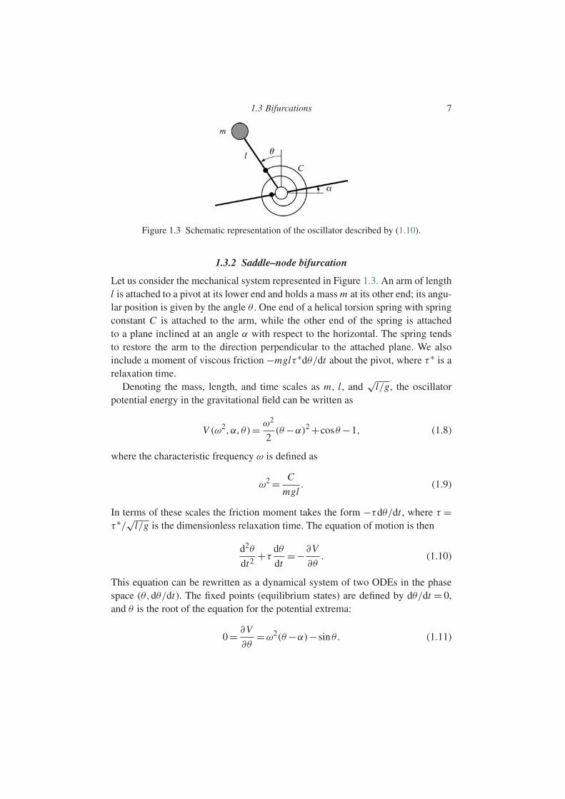
Figure 1.3 Schematic representation of the oscillator described by (1.10).

1.3.2 Saddle–node bifurcation

Let us consider the mechanical system represented in Figure 1.3. An arm of lengthl is attached to a pivot at its lower end and holds a mass m at its other end; its angu-lar position is given by the angle θ . One end of a helical torsion spring with springconstant C is attached to the arm, while the other end of the spring is attachedto a plane inclined at an angle α with respect to the horizontal. The spring tendsto restore the arm to the direction perpendicular to the attached plane. We alsoinclude a moment of viscous friction −mglτ ∗dθ/dt about the pivot, where τ ∗ is arelaxation time.

Denoting the mass, length, and time scales as m, l, and√

l/g, the oscillatorpotential energy in the gravitational field can be written as

V (ω2,α,θ)= ω2

2(θ −α)2 +cosθ −1, (1.8)

where the characteristic frequency ω is defined as

ω2 = C

mgl. (1.9)

In terms of these scales the friction moment takes the form −τdθ/dt , where τ =τ ∗/

√l/g is the dimensionless relaxation time. The equation of motion is then

d2θ

dt2+τ

dθ

dt=−∂V

∂θ. (1.10)

This equation can be rewritten as a dynamical system of two ODEs in the phasespace (θ,dθ/dt). The fixed points (equilibrium states) are defined by dθ/dt = 0,and θ is the root of the equation for the potential extrema:

0= ∂V

∂θ=ω2(θ −α)−sinθ. (1.11)

8 Introduction

(a)

V

θ

θeq

(b)

α > αc

–αc αc α

α > 0

α = 0

α < 0

α < –αc

Figure 1.4 (a) The potential V (θ) for various inclinations α (the relative verticalpositions of the various curves are arbitrary). (b) The bifurcation diagram: (—)stable states, (- -) unstable states.

The dependence of the equilibrium states on the two parameters ω2 and α canbe determined graphically or, for |α| small and ω2 near unity, by a Taylor seriesexpansion about θ = 0. For α = 0 the potentials at the equilibrium points θ− andθ+ are the same (Figure 1.4a). For |α| small and ω2 < 1 the system possesses anunstable equilibrium state θ0 near θ =0 (the corresponding fixed point is a saddle)and two stable equilibrium states on either side, θ− < 0 and θ+ > 0 (whose corre-sponding fixed points are nodes). For α<0 the state θ−<0 has the lowest potentialand is therefore the most stable state, while the state θ+>0 is only metastable. Thesituation is reversed for α>0.

Let us consider the system in the state θ− with α positive and small (Figure1.4b). As α increases, the metastable equilibrium state θ− and the unstableequilibrium state θ0 approach each other, and there exists a critical inclina-tion αc for which the two equilibrium states merge. For α > αc, the systemjumps to the stable branch θ+. For α = αc, the phase portrait of the systemtherefore undergoes a qualitative change when the stable node (θ−,0) and theunstable saddle (θ0, 0) coalesce. This qualitative change corresponds to a bifur-cation: for α = αc, an eigenvalue of the system linearized about each of thefixed points (θ0, 0) and (θ−,0) crosses the imaginary axis (the proof is left asan exercise). The corresponding bifurcation is called a saddle–node bifurcation.A similar bifurcation occurs for decreasing α when α reaches the value −αc.Figure 1.4b, which shows the fixed points as a function of the parameter α, iscalled the bifurcation diagram. At each bifurcation the system jumps from onebranch to another, and the critical value of the bifurcation parameter α is dif-ferent depending on whether it is increasing or decreasing: the system displayshysteresis.

1.3 Bifurcations 9

Figure 1.5 The saddle–node bifurcation diagram: (—) stable states, (- -) unstablestates.

This example2 displays a bifurcation corresponding to the coalescence of twofixed points, called a saddle–node bifurcation. The general definition of such abifurcation is the following.

Definition 1.2 A dynamical system possessing a stable fixed point a undergoesa saddle–node bifurcation at µ=µc if a real eigenvalue of the system linearizedabout a crosses the imaginary axis for µ=µc. For µ in the neighborhood of µc,the behavior of the system is then governed, maybe after an appropriate changeof variables, by the following equation, called the normal form of a saddle–nodebifurcation:

dx

dt=µ− x2. (1.12)

Figure 1.5 shows the corresponding bifurcation diagram.

1.3.3 Pitchfork bifurcation

Let us return to the oscillator of Figure 1.3, and now consider what happenswhen we allow ω2 to vary for fixed α = 0. As ω2 increases, the potential bar-rier between the two minima flattens, and the three equilibrium points coalescefor ω2

c0 = 1 (Figure 1.6a). For ω2 >ω2c0, only the stable equilibrium state θ = 0

exists. This qualitative change of the phase portrait again corresponds to a bifur-cation: for ω2 =ω2

c0, an eigenvalue of the system linearized about (0,0) crossesthe imaginary axis (the proof is left as an exercise). The corresponding bifurca-tion is called a supercritical pitchfork bifurcation and the bifurcation diagram isshown in Figure 1.6b. The term supercritical means that in passing through thebifurcation a stable branch of equilibrium positions varies continuously, withoutany discontinuity.

2 An extension of the analysis to the case of a chain of coupled oscillators can be found in Charru (1997).

10 Introduction

(a) (b)

Vω > ωc0

ω = ωc0

ω < ωc0

θ

θeq

ωc0 ω

Figure 1.6 (a) The potential for various ω and α=0 (the relative vertical positionsof the various curves are arbitrary). (b) Bifurcation diagram: (—) stable states,(- -) unstable states.

The existence of the pitchfork bifurcation displayed in this example is related ina crucial way to the symmetry of the problem about θ =0, i.e., to the invariance ofthe equation for the transformation of θ into −θ , which is referred to as reflectioninvariance. A pitchfork bifurcation is defined more generally as follows.

Definition 1.3 A dynamical system which is invariant under reflection, i.e.,invariant under the transformation x → −x (associated with a symmetry of thephysical system), and which possesses a stable fixed point a undergoes a pitchforkbifurcation at µ=µc if a real eigenvalue of the system linearized about a crossesthe imaginary axis for µ=µc. For µ in the neighborhood of µc, the behavior ofthe system is then governed, perhaps after an appropriate change of variables, bythe following equation, called the normal form of a pitchfork bifurcation:

dx

dt=µx −δx3, δ=±1. (1.13)

The case δ=1 is termed supercritical and the case δ=−1 is termed subcritical.

Figure 1.7 shows the corresponding bifurcation diagrams. In the supercriticalcase the equilibrium state x = 0 is stable for µ< 0 and unstable for µ> 0; in thelatter case any perturbation of this equilibrium state makes the system jump to oneof the stable branches ±√

µ. In the subcritical case and for µ<0, x =0 is alwaysstable with respect to infinitesimal amplitude perturbations, but an amplitudeperturbation larger than ±√−µ, i.e., a perturbation of finite amplitude, can desta-bilize it: for µ> 0, any perturbation of the state x = 0 causes the system to jumpdiscontinuously to a state that the normal form (1.13) is incapable of describing;higher-order terms (of degree five or higher) must be taken into account.

What happens in a system when the reflection symmetry x → −x is brokenby an imperfection? We return to the oscillator of Figure 1.3 but now for small,nonzero angle α, which breaks the θ →−θ invariance, and we consider the effect

1.3 Bifurcations 11

Figure 1.7 Pitchfork bifurcation diagrams: (a) supercritical (δ = +1), (b) sub-critical (δ=−1); (—) stable states, (- -) unstable states.

(a) (b)

V

ω > ωc

θeq

θ

ω < ωc

ωc

ω

Figure 1.8 (a) The potential for ω<ωc and ω>ωc, for α =0. (b) Bifurcation dia-gram: (—) stable states, (- -) unstable states. A saddle–node bifurcation survivesfor ω=ωc.

of varying ω. For ω small there are still two stable equilibria on either side of anunstable equilibrium, but the positions of stable equilibria are no longer symmet-ric about θ = 0, and the position of the unstable equilibrium is no longer locatedat θ = 0 (Figure 1.8a). As α increases, the two stable branches approach eachother as for α = 0, but they do not coalesce: the lower branch merges with theunstable branch for ω2

c(α) <ω2c0 (Figure 1.8b), and we again arrive at a saddle–

node bifurcation. This example shows that the pitchfork bifurcation is a specialcase corresponding to a system which is invariant under the change of variableθ →−θ , i.e., a system which possesses symmetry under reflection. The breakingof this symmetry causes pitchfork bifurcation to be replaced by saddle–node bifur-cation. The latter is termed generic, as it is robust with respect to additional termsin (1.13) describing imperfections of the physical system in question.

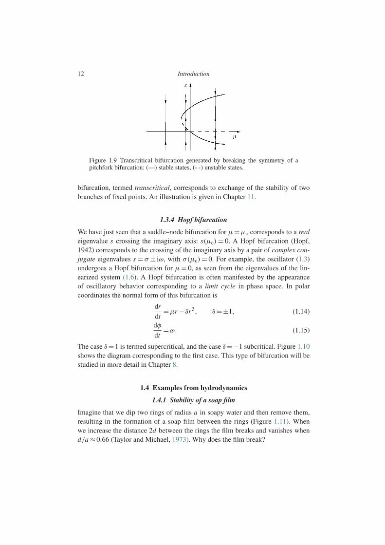
Another type of perturbation of a pitchfork bifurcation can occur; its bifurcationdiagram is shown in Figure 1.9. This other type of symmetry breaking, which hasthe effect of moving the parabolic branches off-center, restores the saddle–nodebifurcation for µ<0, but another bifurcation survives at µ=0. This other type of

12 Introduction

Figure 1.9 Transcritical bifurcation generated by breaking the symmetry of apitchfork bifurcation: (—) stable states, (- -) unstable states.

bifurcation, termed transcritical, corresponds to exchange of the stability of twobranches of fixed points. An illustration is given in Chapter 11.

1.3.4 Hopf bifurcation

We have just seen that a saddle–node bifurcation for µ=µc corresponds to a realeigenvalue s crossing the imaginary axis: s(µc) = 0. A Hopf bifurcation (Hopf,1942) corresponds to the crossing of the imaginary axis by a pair of complex con-jugate eigenvalues s = σ ± iω, with σ(µc)= 0. For example, the oscillator (1.3)undergoes a Hopf bifurcation for µ= 0, as seen from the eigenvalues of the lin-earized system (1.6). A Hopf bifurcation is often manifested by the appearanceof oscillatory behavior corresponding to a limit cycle in phase space. In polarcoordinates the normal form of this bifurcation is

dr

dt=µr −δr3, δ=±1, (1.14)

dφ

dt=ω. (1.15)

The case δ=1 is termed supercritical, and the case δ=−1 subcritical. Figure 1.10shows the diagram corresponding to the first case. This type of bifurcation will bestudied in more detail in Chapter 8.

1.4 Examples from hydrodynamics

1.4.1 Stability of a soap film

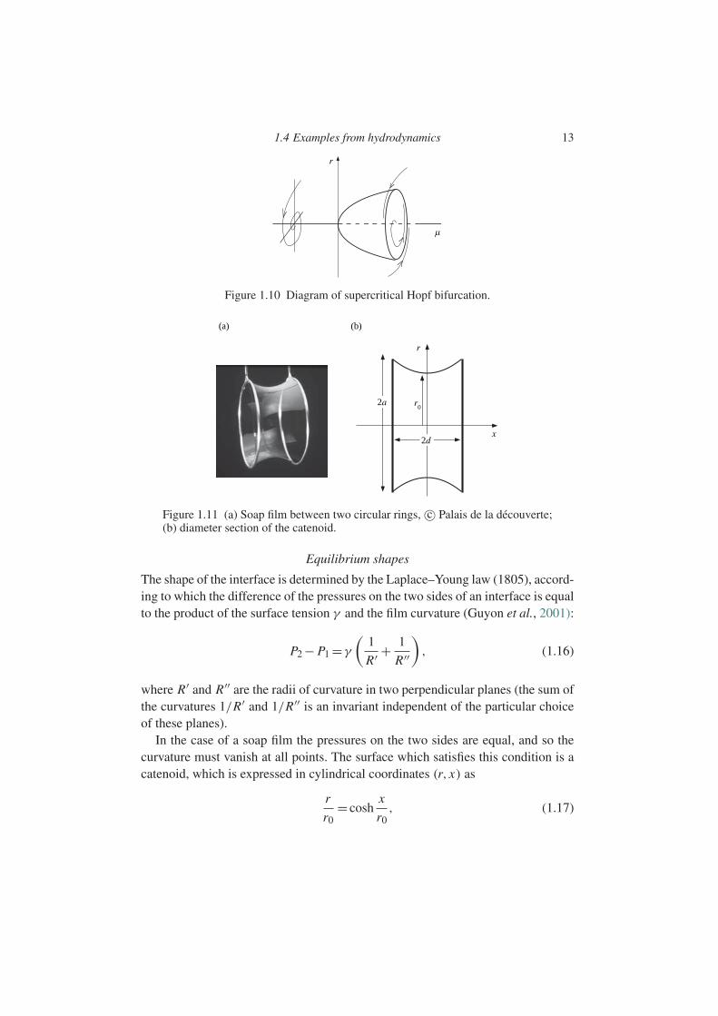
Imagine that we dip two rings of radius a in soapy water and then remove them,resulting in the formation of a soap film between the rings (Figure 1.11). Whenwe increase the distance 2d between the rings the film breaks and vanishes whend/a ≈0.66 (Taylor and Michael, 1973). Why does the film break?

1.4 Examples from hydrodynamics 13

µ

r

Figure 1.10 Diagram of supercritical Hopf bifurcation.

2d

2a

(b)(a)

x

r

r0

Figure 1.11 (a) Soap film between two circular rings, c© Palais de la decouverte;(b) diameter section of the catenoid.

Equilibrium shapes

The shape of the interface is determined by the Laplace–Young law (1805), accord-ing to which the difference of the pressures on the two sides of an interface is equalto the product of the surface tension γ and the film curvature (Guyon et al., 2001):

P2 − P1 =γ

(1

R′ +1

R′′

), (1.16)

where R′ and R′′ are the radii of curvature in two perpendicular planes (the sum ofthe curvatures 1/R′ and 1/R′′ is an invariant independent of the particular choiceof these planes).

In the case of a soap film the pressures on the two sides are equal, and so thecurvature must vanish at all points. The surface which satisfies this condition is acatenoid, which is expressed in cylindrical coordinates (r, x) as

r

r0= cosh

x

r0, (1.17)

14 Introduction

0 0.5 1 1.5 20

1

2

3 (a)

x/r0

r 0/r

0 0.4 0.80

0.5

1 (b)

d/a

r 0

a/

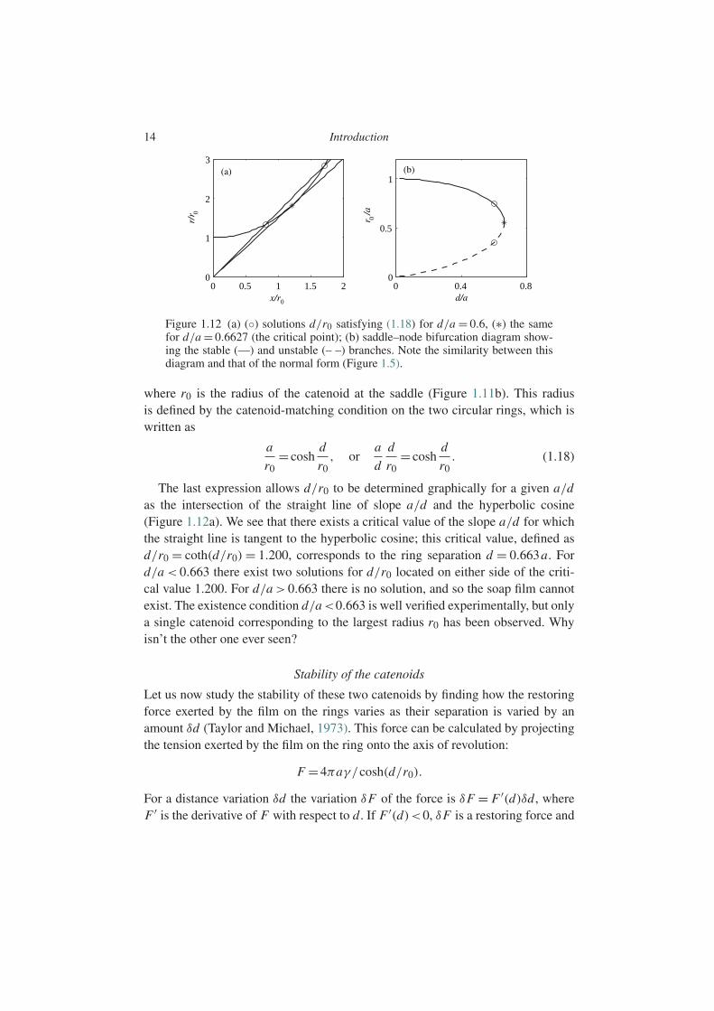
Figure 1.12 (a) () solutions d/r0 satisfying (1.18) for d/a = 0.6, (∗) the samefor d/a = 0.6627 (the critical point); (b) saddle–node bifurcation diagram show-ing the stable (—) and unstable (– –) branches. Note the similarity between thisdiagram and that of the normal form (Figure 1.5).

where r0 is the radius of the catenoid at the saddle (Figure 1.11b). This radiusis defined by the catenoid-matching condition on the two circular rings, which iswritten as

a

r0= cosh

d

r0, or

a

d

d

r0= cosh

d

r0. (1.18)

The last expression allows d/r0 to be determined graphically for a given a/das the intersection of the straight line of slope a/d and the hyperbolic cosine(Figure 1.12a). We see that there exists a critical value of the slope a/d for whichthe straight line is tangent to the hyperbolic cosine; this critical value, defined asd/r0 = coth(d/r0) = 1.200, corresponds to the ring separation d = 0.663a. Ford/a < 0.663 there exist two solutions for d/r0 located on either side of the criti-cal value 1.200. For d/a > 0.663 there is no solution, and so the soap film cannotexist. The existence condition d/a<0.663 is well verified experimentally, but onlya single catenoid corresponding to the largest radius r0 has been observed. Whyisn’t the other one ever seen?

Stability of the catenoids

Let us now study the stability of these two catenoids by finding how the restoringforce exerted by the film on the rings varies as their separation is varied by anamount δd (Taylor and Michael, 1973). This force can be calculated by projectingthe tension exerted by the film on the ring onto the axis of revolution:

F =4πaγ /cosh(d/r0).

For a distance variation δd the variation δF of the force is δF = F ′(d)δd, whereF ′ is the derivative of F with respect to d. If F ′(d)<0, δF is a restoring force and

1.4 Examples from hydrodynamics 15

the film is stable, while in the opposite case the film is unstable. Using (1.18) anddifferentiating to calculate r ′

0(d), we find

F ′(d)= 4πγ

d/r0 −coth(d/r0). (1.19)

F ′(d) is therefore negative for the smaller of the two solutions d/r0 of (1.18), andthe film of larger radius r0 is stable. The other solution of (1.18) corresponds to anunstable film.3 Figure 1.12b shows the variation of the radius at the saddle, r0/a,with distance d/a for the two solutions. We see that the critical value correspondsto coalescence of the stable and unstable branches, and therefore to a saddle–nodebifurcation.

Geoffrey Ingram Taylor (1886–1975)

G. I. Taylor was born in London, England,where his father was a painter and interior dec-orator of ocean liners, and his mother a daugh-ter of George Boole (of Boolean algebra).As a child, he displayed a precocious interestin science and met William Thomson (LordKelvin). He studied at Trinity College, Cam-bridge. His earliest research work included atheoretical study of shock waves (for whichhe won the Smith Prize) and an experimentalstudy inspired by J. J. Thomson to test quan-tum theory. After appointment to the post ofReader in Dynamical Meteorology at Trin-

ity College, he worked on turbulence. After the sinking of the Titanic in1912 he worked as meteorologist on the ship the Scotia assigned to icebergsurveillance in the North Atlantic, where his measurements of temperature,

3 The more complete stability calculation of Taylor and Michael (1973) uses the calculus of variations. Theshorter calculation presented here does not require calculation of the second derivative of the area of thecatenoid

A =2πr20

(d

r0+ 1

2sinh

2d

r0

).

We note that the force variation δF can also be written as δF = −E ′′p (d)δd, where Ep = γ A is the potential

energy of the film (the free energy). The stability condition is therefore just the condition of convexity of thepotential energy (E ′′

p (d) > 0). Finally, it should be observed that the equilibrium does not correspond to an

extremum of the film energy with respect to variations of d: E ′p(d)=−F =0 (see the exercise in Section 1.6.6

below).

16 Introduction

pressure, and humidity helped him develop a model of turbulent mixing ofair. During World War I he participated in the design and operation of air-planes at the Royal Aircraft Factory at Farnborough, where he studied the stresson propellor shafts and learned to fly airplanes and make parachute jumps.After returning to Trinity College he worked on turbulent flow as applied tooceanography and on the problem of bodies passing through a rotating fluid.In 1923 he was appointed Research Professor by the Royal Society of London,which allowed him to give up teaching. (He was not a natural lecturer andnot much interested in teaching... wrote G. K. Batchelor.a) He carried out manyimportant studies, in particular on the deformation of crystalline materials, andintroduced a new statistical approach to velocity fluctuations in turbulence.Batchelor again: His investigations in the mechanics of fluids and solids cov-ered an extraordinary wide range, and most of them exhibited the originalityand insight for which he was now becoming famous... The nature of his think-ing was like that of Stokes, Kelvin and Rayleigh, although he got more fromexperiments than any one of these three. During World War II he worked onthe propagation of blast waves and continued his research at Cambridge until1972, twenty years after his retirement. His name is associated with severalconcepts in turbulence and hydrodynamical phenomena, as well as three fun-damental instabilities: Couette–Taylor, Rayleigh–Taylor, and Saffman–Taylor.He was elected a Fellow of the Royal Society in 1919, and awarded the RoyalMedal (1933), the Copley Medal (1944), and more than twenty other prizes. Hewas knighted and appointed to the Order of Merit, and elected to membershipin academic societies in many countries, including the USSR and the USA.He published over 250 papers in applied mathematics, mathematical physics,and mechanical and chemical engineering. He was keenly interested in botany,traveling, and sailing, and made numerous voyages with his wife in their boat.b

a G. K. Batchelor (1976), Geoffrey Ingram Taylor, Biographical Memoirs of Fellows of the Royal Society ofLondon 22, 565–633.

b This biographical note, like others in this book, has been adapted from the excellent site The MacTu-tor History of Mathematics of J. J. O’Connor and E. F. Robertson, St. Andrews University, Scotland:http://www-history.mcs.st-andrews.ac.uk/. The photograph also comes from this site. For a historicalperspective, see also Darrigol (2005).

1.4.2 Stability of a bubble

Let us consider a bubble of radius r in a liquid at pressure p and temperatureT (Figure 1.13). The bubble contains a mixture of vapor of the liquid and anincondensible gas (air, for example). How do the radius and stability of the bubblevary as the pressure or temperature of the surrounding liquid varies?

1.4 Examples from hydrodynamics 17

Liquid, p, T

Bubble of radius r

Vaporand gas,

pv + pg, T

Figure 1.13 A bubble of vapor and incondensable gas in a liquid.

Equilibrium radii

Assuming that the mixture is ideal, the pressure in the bubble is the sum of thepressure pg of the incondensible gas and the pressure pv(T ) of the vapor in equi-librium with the liquid (the saturation vapor pressure).4 The Laplace–Young lawand the isothermal evolution of the gas (assumed perfect) give the relation betweenthe pressure and the radius:

p(r)= pv(T )+ pg − 2γ

r, pg = pg0

r30

r3, (1.20)

where the subscript 0 denotes a reference state of the bubble. For r sufficientlysmall the 1/r3 term dominates and the pressure p(r) decreases with r . For r suf-ficiently large it is the other term, proportional to −1/r , that dominates, and thepressure p(r) is an increasing function of r . The curve p = p(r) therefore has aminimum corresponding to a radius rc and pressure pc in the liquid given by

rc =(

3pg0r30

2γ

)1/2

, pc = pv − 4γ

3rc.

Choosing rc and γ /rc as the length and pressure scales, the relation betweenpressure and radius becomes

p− pv(T )

γ /rc= 2

3

(rc

r

)3 −2rc

r,

as illustrated in Figure 1.14. We note that for r/rc > 0.6 the pressure p is lowerthan the saturation pressure pv(T ) (and possibly negative), and from the viewpointof thermodynamics the liquid is in metastable equilibrium.

4 Here we ignore the shift of the liquid–vapor equilibrium curve pv(T ) induced by the surface tension, which isimportant only for bubbles less than a micron in diameter.

18 Introduction

0 1r/rc

(p–

p v(T))

/(γ

/rc)

2 3–2

0

2

4

Gas bubble

Vapor bubble

Figure 1.14 Variation of the pressure (p − pv(T ))/(γ /rc) with the equilibriumradius r/rc of a bubble; (—) stable bubbles of incondensable gas, (- -) unstablebubbles of vapor. The minimum corresponds to a saddle–node bifurcation.

Stability from the mechanical point of view

The stability of the equilibrium states can be studied by evaluating the net forceacting on a half-bubble perturbed from its equilibrium radius r . A perturbationδr of this radius is associated with a perturbation δpg of the pressure pg + pv(T )

of the bubble (the saturation vapor pressure pv depends only on temperature andtherefore is not changed in a slow perturbation). The net force on the half-bubbledirected toward the outside is then(

(pv(T )+ pg +δpg)− p)π(r +δr)2 −γ 2π(r +δr).

Linearizing about the equilibrium radius, this becomes

2πγ δr +πr2δpg. (1.21)

For r rc the pressure inside the bubble is dominated by the pressure pg, as thevapor pressure is negligible. The bubble behaves like a bubble of incondensiblegas for which the pressure varies with radius as δpg/pg +3δr/r =0 for isothermalevolution. The linearized net force then becomes

(2πγ −3πr pg)δr =−(2pg + p)πrδr.

This force, of opposite sign to δr , is therefore a restoring force and the bubble isstable (the same result is obtained in the case of isentropic evolution).

For r rc the pressure inside the bubble is now dominated by the vapor pressurepv and the gas pressure is negligible. This bubble behaves like a vapor bubblewhose pressure is determined by the temperature. The net force (1.21) acting on

1.4 Examples from hydrodynamics 19

a half-bubble then reduces to the term 2πγ δr . This force, which has the samesign as δr , therefore tends to amplify the initial perturbation, and so the bubble isunstable.

Stability from the thermodynamic point of view

From the thermodynamic point of view, the first thing to note is that the slope ofthe curve p(r) is related to the isothermal compressibility of the bubble as

κT =− 1

V

∂V

∂p=−3

1

r

∂r

∂p.

This compressibility is positive on the decreasing branch of Figure 1.14, divergesat the minimum, and then is negative on the growing branch. According to ageneral result of thermodynamic stability (Callen, 1985), the decreasing branchcorresponds to stable equilibrium states and the increasing branch to unstable ones.We therefore recover the result of the mechanical analysis performed above.

The general result of thermodynamic stability for the sign of the compressibil-ity follows from the second law of thermodynamics regarding the increase of theentropy of an isolated system. This result can be rederived for the particular casestudied here by considering not the entropy (the bubble is not an isolated system),but rather the free energy F of the system consisting of the bubble and a thin liq-uid film of condensed vapor.5 Let us consider the simple case of a vapor bubble.This bubble is in contact with a heat bath which determines its temperature (butnot its pressure, owing to the surface tension). Under a variation dV of its vol-ume, the variation dF of its free energy is then equal to the work δWrev =−pdVdone by the external forces. We therefore find d(F + pV )= 0, i.e., the functionF + pV is an extremum. This function can be expressed as a function of the bubbleradius as

F + pV =−pvV +γ A+ F0 + pV =−(pv − p)4πr3

3+γ 4πr2 + F0,

where A is the bubble area and F0 is a reference free energy which involves thechemical potential but not the bubble radius. The equilibrium condition

∂(F + pV )

∂r=0

5 Consideration of the film of condensed vapor makes it possible to assume that the bubble has constant mass.We could also use the fact that the liquid imposes a chemical potential µ and then work with the grand potential= F −µN .

20 Introduction

again gives the Laplace–Young law. The bubble potential F + pV then grows asr2 for radii smaller than the equilibrium radius, and as −r3 for radii larger than it.The potential extremum is a maximum, and so the equilibrium of the vapor bubbleis unstable.

In conclusion, the minimum of the curve p(r) in Figure 1.14 corresponds to themerging of two branches of equilibrium states, one stable and the other unstable.This minimum therefore corresponds to a saddle–node bifurcation.

A numerical illustration

As a numerical illustration, let us consider a bubble of radius r0 =1µm in water atatmospheric pressure p0 =101.3 kPa and temperature T0 =20C. At this tempera-ture the saturation vapor pressure is pv(T0)= 2.3 kPa, and for γ = 0.070 N/m thepressure of the gas inside the bubble is pg0 = 239 kPa. The minimum of the curvep(r) corresponds to rc = 2.3µm and pc = −38.9 kPa. The radius r0 is thereforesmaller than rc and the bubble is stable. Let us see how this equilibrium is affectedby variation of the pressure or temperature.

• When the pressure is decreased at constant temperature, the bubble becomesunstable when the liquid pressure reaches the value pc =−38.9 kPa, where thenegative pressure corresponds to a metastable state. If a larger bubble is presentin the water, i.e., a bubble of radius r0 initially larger than 1µm, it will becomeunstable for a liquid pressure either less negative or positive, but always less thanthe saturation pressure pv(T0) owing to the surface tension.

• When the temperature is raised at constant pressure p0, the bubble becomesunstable when the saturation vapor pressure reaches pv(T ) = pc + 4γ /3rc =142 kPa with pc = p0, or T =110C. This temperature (which is slightly changedwhen the temperature dependence of γ is taken into account) is clearly higherthan the equilibrium temperature T =100C of a planar interface. A bubble ini-tially larger (r0 > 1µm) would become unstable at a temperature below 110C(but always higher than 100C owing to the surface tension).

1.4.3 Stability of a colloidal suspension

Many fluids which appear homogeneous to the naked eye actually contain micron-sized particles suspended in a liquid; such fluids are called colloids or colloidalsuspensions. Some examples are mud (clay particles in water), inks, paint (whitezinc oxide particles in water, for example), fruit juices, and emulsions (waterdroplets in oil or the opposite, such as milk). These suspensions are in generalunstable: the particles tend to regroup themselves to form aggregates called flocs,

1.4 Examples from hydrodynamics 21

and small droplets coalesce to form larger ones. This instability originates in theattractive van der Waals forces between the particles. The range of these forces isvery small, on the order of a micron, but thermal agitation or motion of the liquidcan make the particles approach each other to distances small enough that theseforces become dominant and cause the particles to stick together. Colloids can bestabilized by introducing additives such as polymer molecules or surfactants. Con-versely, flocculation can be encouraged, as is done, for example, in water treatmentplants to separate particles from the liquid.

Here we shall consider the effect of a dissolved salt on the stability of a suspen-sion, a phenomenon originally studied by Faraday (1791–1867). Faraday observedthat a colloid of gold, prepared by rubbing together two gold electrodes immersedin water and connected to an electric battery, is stable.6 Even though they aresubject to van der Waals attraction, the particles in this colloid remain sepa-rated. The reason is that the gold particles spontaneously carry negative chargeson their surfaces which keep the particles far apart owing to electrostatic repul-sion (Figure 1.15a). Faraday attempted to confirm this explanation by dissolvingsodium chloride in the water. The color of the colloid changed from red to blue: thesuspension had become unstable and the particles had formed aggregates. Why hadthis happened? The sodium chloride had dissolved, and the Na+ ions, attracted bythe negatively charged gold particles, stuck to them, thus screening the electrostaticinteraction created by these charges (Figure 1.15b). The repulsive force therebybeing neutralized, the van der Waals force became dominant, and the suspensionflocculated.

--

--

----

++++

++

++

++

- --

-

---

-

-

-

--

--

-- - -

++

++

+

++

++

---

-

- -

--

+

(a)

(b)

--

--

----

--

--

-- - -

FA FAFR FR

Figure 1.15 Forces between two charged spheres: (a) electrostatic repulsiondominates van der Waals attraction and the suspension is stable; (b) the posi-tive ions of a dissolved salt screen the electrostatic force and the attractive forcedominates, making the suspension unstable.

6 Our description of the experiment follows that of de Gennes and Badoz (1994).

22 Introduction

A variation of the Faraday experiment is to observe the effect of adding salt to asuspension of clay particles in water. Like gold particles, clay particles carry neg-ative charge on their surface and the suspension is stable. The particles are heavierthan water and gradually undergo sedimentation. The addition of salt makes thesuspension unstable and causes the particles to flocculate. The sedimentation ratevaries as the square of the particle size (Guyon et al., 2001), and this instability ismanifested as a marked increase in the sedimentation rate of the particles. Try theexperiment yourself!

Let us now perform a more quantitative analysis. For two spheres of radius awhose surfaces are separated by a distance d a, calculation of the van der Waalsattractive interaction potential VA gives

VA =− Aa

12d, (1.22)

where A = 10−19 J is a typical value for the Hamaker constant (Probstein, 2003).The repulsive electrostatic potential VR generated by the double layer of negativeand positive charges decreases very rapidly – exponentially – with distance. In thevicinity of a particle, i.e., up to a distance of the order of the particle radius, thispotential is given by

VR =2πaεφ2we−d/λD, λD =

(εkBT

2z2e2 NAC

)1/2

, (1.23)

where φw is the potential at the particle surface and λD is the Debye wavelength,which corresponds to the range of the electrostatic force of the double layer.7 Thisrange is smaller the larger the ion concentration C ; for an aqueous solution ofmonovalent ions it is about 1 nm for a concentration of 102 mol·m−3 and 10 nmfor one of 1 mol·m−3.

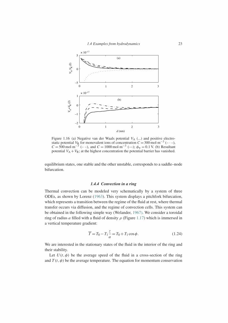
Figure 1.16 shows the shape of the attractive and repulsive potentials VA andVR for three different concentrations, along with the net potential VA + VR inthe three cases. We see that the potential barrier keeping the particles sepa-rate decreases as the concentration increases. The critical concentration abovewhich the suspension is unstable corresponds to the vanishing of the barrier whenthe maximum and minimum coalesce (the minimum, which lies to the right ofthe maximum, is very flat). In terms of dynamical systems, this fusion of two

7 ε is the electrical permittivity of the electrolyte (7.1×1010 C V−1 m−1 for water), kB =1.38×10−23 J K−1 isthe Boltzmann constant, z is the valence of the ions (1 for Na+ and Cl−), e=1.60×10−19 C is the elementaryelectric charge, and NA =6.02×1023 mol−1 is Avogadro’s number.

1.4 Examples from hydrodynamics 23

5

0

–5

–1

–2

0

1

0 1

(a)

(b)

d (nm)

V A+

V R (J

)V A

,VR

(J)

2 3

0 1 2 3

× 10–17

× 10–17

Figure 1.16 (a) Negative van der Waals potential VA (...) and positive electro-static potential VR for monovalent ions of concentration C =300 mol·m−3 (– · –),C = 500 mol·m−3 (– –), and C = 1000 mol·m−3 (—); φw = 0.1 V. (b) Resultantpotential VA +VR; at the highest concentration the potential barrier has vanished.

equilibrium states, one stable and the other unstable, corresponds to a saddle–nodebifurcation.

1.4.4 Convection in a ring

Thermal convection can be modeled very schematically by a system of threeODEs, as shown by Lorenz (1963). This system displays a pitchfork bifurcation,which represents a transition between the regime of the fluid at rest, where thermaltransfer occurs via diffusion, and the regime of convection cells. This system canbe obtained in the following simple way (Welander, 1967). We consider a toroidalring of radius a filled with a fluid of density ρ (Figure 1.17) which is immersed ina vertical temperature gradient:

T = T0 −T1z

a= T0 +T1 cosφ. (1.24)

We are interested in the stationary states of the fluid in the interior of the ring andtheir stability.

Let U (t,φ) be the average speed of the fluid in a cross-section of the ringand T (t,φ) be the average temperature. The equation for momentum conservation

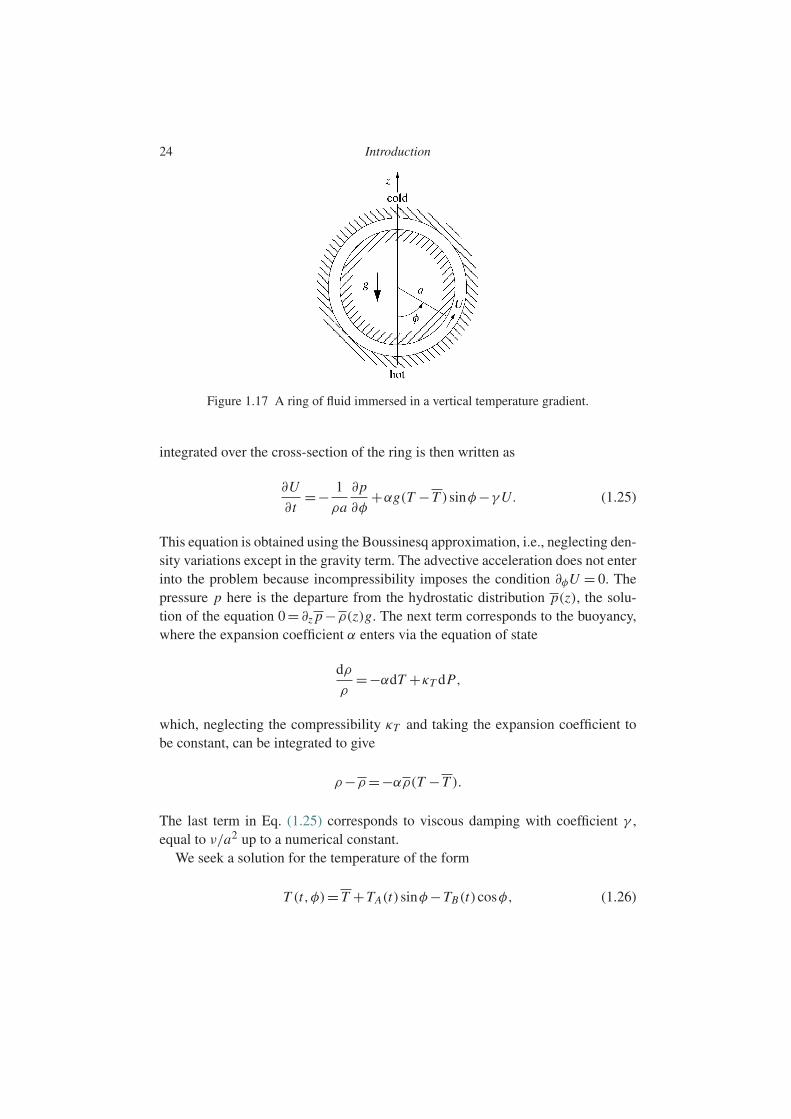
24 Introduction

Figure 1.17 A ring of fluid immersed in a vertical temperature gradient.

integrated over the cross-section of the ring is then written as

∂U

∂t=− 1

ρa

∂p

∂φ+αg(T −T )sinφ−γU. (1.25)

This equation is obtained using the Boussinesq approximation, i.e., neglecting den-sity variations except in the gravity term. The advective acceleration does not enterinto the problem because incompressibility imposes the condition ∂φU = 0. Thepressure p here is the departure from the hydrostatic distribution p(z), the solu-tion of the equation 0 = ∂z p −ρ(z)g. The next term corresponds to the buoyancy,where the expansion coefficient α enters via the equation of state

dρ

ρ=−αdT +κT dP,

which, neglecting the compressibility κT and taking the expansion coefficient tobe constant, can be integrated to give

ρ−ρ =−αρ(T −T ).

The last term in Eq. (1.25) corresponds to viscous damping with coefficient γ ,equal to ν/a2 up to a numerical constant.

We seek a solution for the temperature of the form

T (t,φ)= T +TA(t)sinφ−TB(t)cosφ, (1.26)

1.4 Examples from hydrodynamics 25

where TA(t) and TB(t) are two amplitudes. The pressure can be eliminated fromthe problem by integrating (1.25) from φ=0 to φ=2π . We then obtain

dU

dt= αg

2TA −γU. (1.27)

This equation shows that the temperature difference 2TA between the left and rightbranches acts as a destabilizing forcing term.

The equation for energy conservation is written in simplified form as

∂T

∂t+ U

a

∂T

∂φ= k(T −T ). (1.28)

The left-hand side represents the material derivative of the temperature, and theright-hand side corresponds to heat transfer to the surroundings. Viscous dissipa-tion is neglected, as is the coefficient affecting the advection term (the average ofa nonlinear term is not equal to a product of averages). Taking into account (1.26)and the fact that (1.28) must be satisfied for all φ, we obtain the two differentialequations governing TA and TB :

dTA

dt=−U

a(TB −T1)−kTA, (1.29a)

dTB

dt= U

aTA −kTB . (1.29b)

The differential equations (1.27) and (1.29) form a dynamical system with threedegrees of freedom, U , TA, and TB , which is nonlinear (the nonlinearities arisefrom the advection of the temperature by the flow). After a change of scale

X = 1

kaU, Y = αg

2γ kaTA, Z = αg

2γ kaTB, τ = kt, (1.30)

this system becomes

dX

dτ=−P X + PY, (1.31a)

dY

dτ=−Y − X Z + R X, (1.31b)

dZ

dτ=−Z + XY, (1.31c)

where the parameters P and R, defined as

P = k

γ, R = αgT1

2γ ka,

26 Introduction

are analogs of the Prandtl and Rayleigh numbers. The system (1.31) is identical tothat obtained by Lorenz (1963) for describing atmospheric motions in a simplifiedmanner. His landmark study showed that a system with three degrees of freedomcan display disordered, “unpredictable” behavior, and played an important role inunderstanding deterministic chaos (Lighthill, 1986; Berge et al., 1987; Schusterand Wolfram, 2005).

The fixed points of the dynamical system (1.31) are (X,Y, Z)= (0,0,0), corre-sponding to the fluid at rest, and, for r = R −1 positive, (X,Y, Z)= (±√

r ,±√r ,r),

corresponding to steady rotation of the fluid in one or the other direction.Let us study the linear stability of the fixed point corresponding to the fluid at

rest. Linearizing (1.31) about (0,0,0), we obtain a linear system with a constant-coefficient matrix L which has solutions of the type exp(sτ). The resulting systemof equations has a nontrivial solution only if the determinant of L− sI vanishes,leading to

(s +1)(

s2 +(P +1)s −r P)=0. (1.32)

It is easy to verify that the roots of the second-degree polynomial are real and bothnegative for r < 0 (R < 1), or of opposite signs for r > 0 (R > 1). We thereforeconclude that the rest state is stable for r <0 and unstable for r >0.

The stability of the other two branches of fixed points is studied in the samemanner. The characteristic polynomial, which is the same for the two branches, is

s3 +(P +2)s2 +(P +1+r)s +2r P =0. (1.33)

Near the threshold r = 0 of instability of the fluid at rest we can seek solutions inthe form of a series in powers of r , s = s(0)+rs(1)+·· · , which leads to

s1 =− 2r P

P +1+O(r2), (1.34a)

s2 =−1+O(r), (1.34b)

s3 =−(P +1)+O(r). (1.34c)

These three roots are negative, the branches (X,Y, Z) = (±√r ,±√

r ,r) aretherefore stable, and the bifurcation at r =0 is a supercritical pitchfork bifurcation.

We can go further by noting that the characteristic polynomial (1.33), whichhas the form s3 + As2 + Bs +C = 0, has positive real coefficients. A real root canonly be negative, and so an instability necessarily corresponds to a complex roots = sr + isi. The instability threshold of the branches (X,Y, Z)= (±√

r ,±√r ,r)

therefore corresponds to sr =0. We thereby demonstrate that for P <2 the branches(X,Y, Z) = (±√

r ,±√r ,r) are stable for all R, and for P > 2 they become

unstable for R = P(P +4)/(P −2) via a Hopf bifurcation (Glendinning, 1994).

1.4 Examples from hydrodynamics 27

1.4.5 Double diffusion of heat and matter

The presence of a concentration gradient of dissolved salt together with a temper-ature gradient leads to remarkable instability phenomena such as the developmentof salt fingers. This particular phenomenon, which is illustrated in Figure 1.18,occurs in a fluid with stabilizing (positive) temperature gradient when the salt con-centration is higher on the top than on the bottom. Since salt water is denser thanfresh water, this distribution of the salt concentration is unstable, thus leading tothe observed fingers.

Here we consider the different situation of a statically stable mixture of saltand water, i.e., a mixture with a concentration profile C(z) such that the densitydecreases with height, and investigate the effect of a temperature gradient thatcan be either positive or negative. The density is given by the equation of stateρ = ρ(P,T,C) which, neglecting compressibility, can be written in differentialform as

dρ

ρ=−αdT +βdC, (1.35)

where α>0 is the thermal expansion coefficient and β >0 is an analogous coeffi-cient describing the variation of the density with the salt concentration. Near anyreference height z0 the concentration profile is

C(z)=C0 +C ′0(z − z0),

Figure 1.18 Descending fingers of salt water, formed by pouring a salt watersolution into fresh water possessing a stabilizing (positive) temperature gradi-ent. The fingers are rendered visible by adding fluorescein to the salt water andilluminating it from below through a slit (Huppert and Turner, 1981).

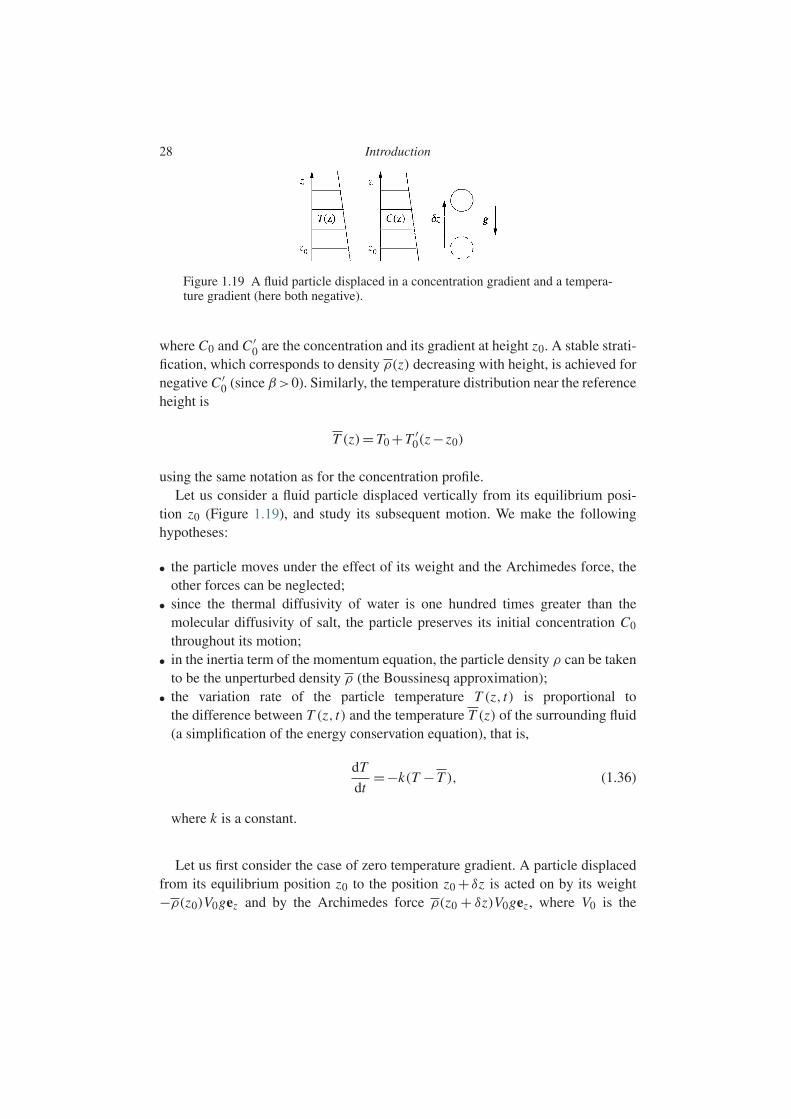
28 Introduction

Figure 1.19 A fluid particle displaced in a concentration gradient and a tempera-ture gradient (here both negative).

where C0 and C ′0 are the concentration and its gradient at height z0. A stable strati-

fication, which corresponds to density ρ(z) decreasing with height, is achieved fornegative C ′

0 (since β>0). Similarly, the temperature distribution near the referenceheight is

T (z)= T0 +T ′0(z − z0)

using the same notation as for the concentration profile.Let us consider a fluid particle displaced vertically from its equilibrium posi-

tion z0 (Figure 1.19), and study its subsequent motion. We make the followinghypotheses:

• the particle moves under the effect of its weight and the Archimedes force, theother forces can be neglected;

• since the thermal diffusivity of water is one hundred times greater than themolecular diffusivity of salt, the particle preserves its initial concentration C0

throughout its motion;• in the inertia term of the momentum equation, the particle density ρ can be taken

to be the unperturbed density ρ (the Boussinesq approximation);• the variation rate of the particle temperature T (z, t) is proportional to

the difference between T (z, t) and the temperature T (z) of the surrounding fluid(a simplification of the energy conservation equation), that is,

dT

dt=−k(T −T ), (1.36)

where k is a constant.

Let us first consider the case of zero temperature gradient. A particle displacedfrom its equilibrium position z0 to the position z0 + δz is acted on by its weight−ρ(z0)V0gez and by the Archimedes force ρ(z0 + δz)V0gez , where V0 is the

1.4 Examples from hydrodynamics 29

constant volume of the particle. Its equation of motion is then

d2

dt2δz = gβC ′

0δz.

For C ′0 < 0 the net vertical force is a restoring force which gives rise to neutral

oscillations of the particle with frequency N =√

−gβC ′0, called the Brunt–Vaisala

frequency.Let us now assume a nonzero temperature gradient T ′

0. A particle displaced adistance δz is subject to its weight −ρ(z0)V0gez , as before, and the Archimedesforce ρ(z0 + δz)(V0 + δV )gez , where δV = V0αδT is the variation of the particlevolume associated with the temperature variation δT = T − T0. The equation ofmotion becomes

d2

dt2δz =αgδT +βC ′

0gδz. (1.37)

Introducing the temperature variation δT into the energy conservation equation(1.36), the latter becomes

d

dtδT =−kδT +kT ′

0δz. (1.38)

The system (1.37)–(1.38) is a system of linear differential equations with constantcoefficients, and has nonzero exponential solutions of the form exp(st) when theeigenvalue s is a solution of the characteristic polynomial

(s +k)(s2 + N 2)−αgkT ′0 =0. (1.39)

For a weak temperature gradient T ′0 we can seek the eigenvalues as perturbations

s′ of the eigenvalues ±iN corresponding to zero temperature gradient, that is, s =±iN +s′. We then find

s′± = −N ± ik

2N (N 2 +k2)αgkT ′

0. (1.40)

The imaginary part of these eigenvalues corresponds to a shift of the Brunt–Vaisalafrequency. The real part provides the answer for the stability: for positive tempera-ture gradient T ′

0, the real part is negative and the oscillation decays; conversely, fornegative temperature gradient T ′

0, the oscillation amplifies and the stratification isunstable. For T ′

0 = 0 the pair of complex-conjugate eigenvalues crosses the imag-inary axis at ±N , which is none other than a Hopf bifurcation. This result can beinterpreted physically by noting that for T ′

0 < 0 the particle is subject not only to

30 Introduction

the restoring force due to the concentration gradient which produces an oscillationat frequency N , but also to an additional destabilizing force associated with thetemperature gradient. Accordingly, as the particle passes through its equilibriumposition z0, say, from below, it is hotter and lighter than the surrounding fluid. It isthen pulled upwards by the buoyancy force and overshoots the previous maximum,so that the oscillation amplitude increases.

1.5 Non-normality of the linearized operator

1.5.1 Algebraic transient growth

Strictly speaking, any study of linear stability is incomplete if it deals onlywith the asymptotic stability of an equilibrium state under “infinitesimal” ampli-tude perturbations. In the real world, perturbations (various types of fluctuation,vibrations, etc.) have a finite amplitude. Fortunately, it has been proved that formany physical systems the predictions of linear stability analysis are well con-firmed experimentally for amplitudes (normalized by a scale characteristic ofthe problem) of order 10−2 or even 10−1, for which nonlinear effects remainnegligible. However, the domain of validity of the linear analysis is sometimeslimited to amplitude perturbations which are extremely small, perhaps of order10−3, smaller than the ordinary ambient “noise,” and so, except in experimentswhere noise effects are really under control, the predictions may not agree withobservation.

Noise effects are particularly important in the neighborhood of a subcriticalbifurcation. Let us consider the simple case of a subcritical pitchfork bifurcationwhose normal form is given by Eq. (1.13) with δ = −1. As seen from the bifur-cation diagram, for µ < 0 the equilibrium state x = 0 is stable with respect toinfinitesimal perturbations but unstable if the initial amplitude is larger than

√−µ.Therefore, if the system is subject to noise of characteristic amplitude ε, the bifur-cation for µ increasing will occur for µ≈ −ε2, not for µ= 0. Experimentally, aspread in the measured bifurcation thresholds associated with the random natureof the noise is observed.

The phenomenon described above becomes dramatic for systems in which cer-tain perturbations, even though they decay exponentially at long times, can displaytransient growth. Such transient growth can amplify the initial energy of the pertur-bation by extremely large factors of 102 or 103 or more. Nonlinear effects may thenbecome significant and can eventually destabilize the system. This phenomenonis related to non-normality of the linearized operator, i.e., to the nonorthogonalnature of the eigenvectors (for a more complete introduction to this problem, seeTrefethen et al. (1993) and Schmid and Henningson (2001, §4)).

1.5 Non-normality of the linearized operator 31

In order to illustrate the above ideas, let us consider the linear dynamical system

dxdt

=Ax, A=(

0 10 0

), (1.41)

where A is a Jordan block. This system possesses a double-zero eigenvalue asso-ciated with the unique eigenvector e = (1,0). The solution of this system for theinitial condition (x10, x20) is

x1 = x20t + x10, x2 = x20.

The solution therefore grows with time not exponentially, but algebraically.Let us now consider the “perturbed” system

dxdt

=Ax, A=(−ε 1

0 −2ε

), 0<ε 1. (1.42)

The origin (0,0) is the only fixed point of this system and it is stable: the eigenval-ues are −ε and −2ε, with eigenvectors e1 = (1,0) and e2 = (1,−ε), respectively.We note that the angle between these two vectors is small, of order ε. The solutionof this system for the initial condition (x10, x20) is

x= y10 e−εt e1 + y20 e−2εt e2, y10 = x10 + x20

ε, y20 =− x20

ε, (1.43)

where y10 and y20 are the initial conditions in the basis of the eigenvectors. Thephase portrait is shown in Figure 1.20: since the eigenvalues are nonorthogonal,the trajectories are initially parallel to the more stable eigendirection e2; they thenconverge toward the fixed point following the less stable eigendirection e1.

How, for ε tending to zero, does the exponential decay match up with the alge-braic growth at ε=0? In order to answer this question, let us study how the energyE(t)=x(t)·x(t) of the perturbation varies with time. At long times, i.e., for εt 1,the behavior of the solution (1.43) is no surprise: the component in the most stabledirection e2 is exponentially small, and the solution becomes

x∼ y10 e−εt e1,

for which the energy decreases exponentially.8 At short times (εt 1), a Taylorseries expansion of the energy gives

E(t)= (y10 + y20)2 +(εy20)

2 −(2y210 +4(1+ε2)y2

20 +6y10y20)εt +O(ε2t2).

(1.44)

8 Here the symbol ∼ is used in the sense of asymptotic equivalence (Hinch, 1991).

32 Introduction

Figure 1.20 Phase portrait of the dynamical system (1.42), with a stable fixedpoint at the origin. Initial conditions in the hatched region lead to transient growth.

This expansion shows that the energy can grow if the coefficient of εt is nega-tive, which can happen for particular initial conditions to be determined. Since thedynamical system is linear, there is no loss of generality if we take y10 to be strictlypositive and set y20 =−ay10 (the special case y10 =0 corresponds to trivial decayalong the most stable eigendirection). Analysis of the sign of the coefficient of εtthen shows that a necessary condition for growth at short times is ε2 < 1/8, andthat the initial conditions for which the energy is amplified are such that

a− <a <a+, with a± = 3±√1−8ε2

4(1+ε2). (1.45)

Therefore, in the phase space, all initial conditions located in the sector delimitedby the straight lines of slope −a− and −a+ in the eigenvector basis (i.e., for smallε, the lines x20 ∼ εx10 and x20 ∼ (1/2ε)x10) give rise to transient growth of theenergy.

The phase portrait shown in Figure 1.20 explains the situation geometrically.Initial conditions “downstream” of the hatched region lead to exponential decayto the origin (the norm of the vector x, and therefore of the energy x·x, decreasesmonotically). Initial conditions within the hatched region lead first to transientgrowth, and then, as the point exits the hatched region, to exponential decay.Finally, for initial conditions “upstream” of the hatched region, the energy firstdecays then grows, and eventually decays. We emphasize the fact that this growthat short times can only be transient, and that at long times the exponential decaywill eventually prevail.

We can next ask which of the above initial conditions corresponds to the largesttransient growth. This particular initial condition, called the “optimal perturbation”in control theory, is obtained in two steps. The first is to find the time at which theenergy E(t) associated with a given initial condition passes through a maximum;

1.5 Non-normality of the linearized operator 33

by differentiation we find that this time tmax is

εtmax = lna

a−, a− ≤a ≤a+.

The relation between the maximum E(tmax) and the initial energy E0, referredto as the “gain,” is then

E(tmax)

E0= a2−

a2

(1+ε2)a2−−2a−+1

(1+ε2)a2 −2a +1. (1.46)

The second step is to find the initial condition which maximizes this gain. We find,again by differentiation, that this optimal condition corresponds to

aopt =a+, or x20 ∼ x10

2ε.

In Figure 1.20, this line corresponds to the edge with highest slope of the hatchedregion, with a clear geometrical interpretation. It should be noted that the optimalperturbation is located on a direction close to the normal to the eigendirections; weshall return to this later. Then the maximal gain is

maxa

(E(tmax)

E0

)= (3a−−1)(1−a−)

(3a+−1)(1−a+). (1.47)

It can be verified that the optimal perturbation, giving the maximum gain, corre-sponds to zero initial growth rate, i.e., dx2/dt = 0 at time t = 0. This maximumgain depends only on ε and is larger the smaller ε is. For example, it reaches 625for ε=10−2 and 62,500 for ε=10−3. Figure 1.21 shows the time evolution of theenergy for ε=0.1, normalized by the initial energy, for two initial conditions. One,for y20 =−a−y10, leads to monotonic decrease of the energy, while the other, fory20 =−aopty10, corresponds to the optimal condition maximizing the gain.

In conclusion, certain perturbations of an asymptotically stable equilibrium statecan be strongly amplified in a transient manner by a purely linear effect. This tran-sient growth is essentially related to the nonorthogonal nature of the eigenvectorsof the system linearized at the fixed point. The optimal perturbation is oriented ina direction normal to the neighboring eigendirections.

1.5.2 Optimal excitation of an unstable mode

The above discussion of the possibility of transient growth concerns an equilibriumstate which is linearly stable. In the case of an unstable equilibrium state, i.e., for asystem with an eigenvalue which has positive real part, a related question is that ofthe “optimal excitation” of the unstable mode (Farrell, 1988). This optimal exci-tation corresponds to the initial perturbation which allows, at a given instant, the

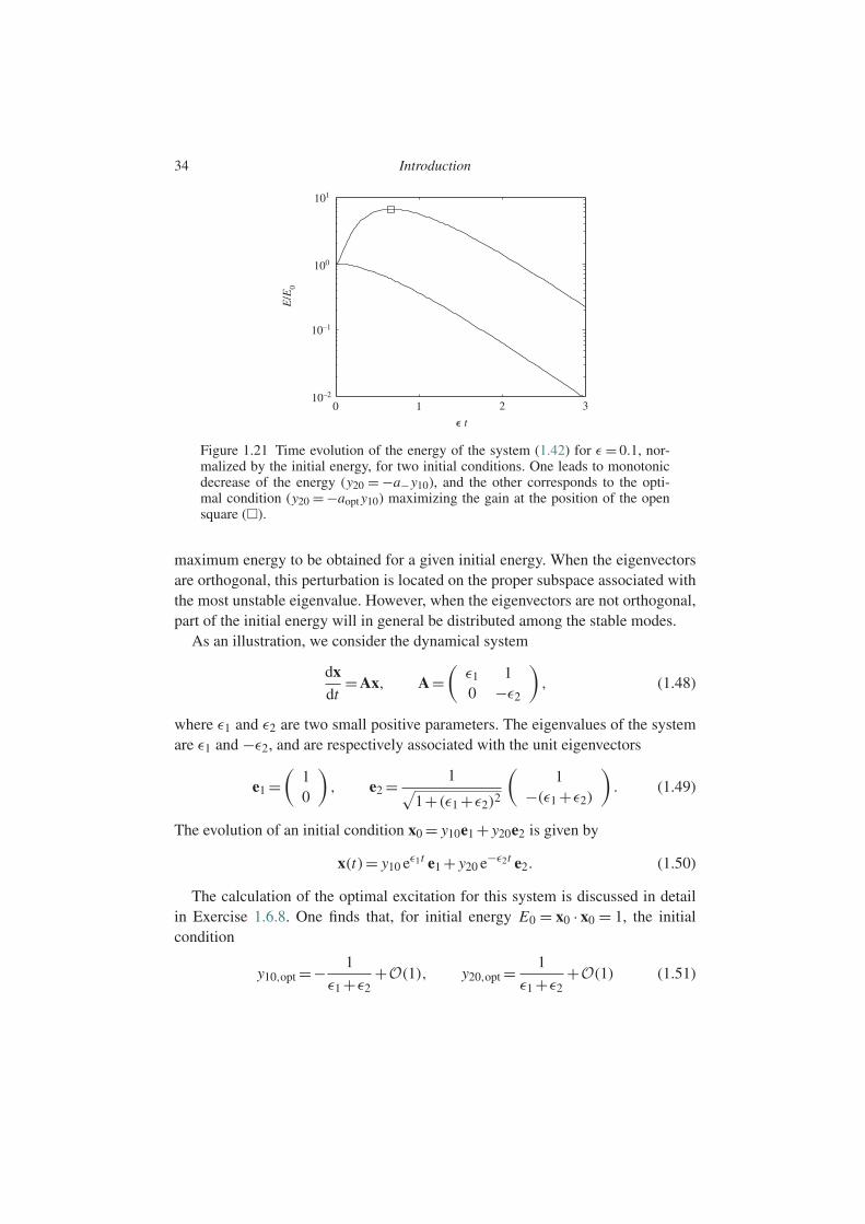
34 Introduction

101

100

10–1

10–2

0 1

E/E

0

2 3

e t

Figure 1.21 Time evolution of the energy of the system (1.42) for ε = 0.1, nor-malized by the initial energy, for two initial conditions. One leads to monotonicdecrease of the energy (y20 = −a−y10), and the other corresponds to the opti-mal condition (y20 = −aopt y10) maximizing the gain at the position of the opensquare ().

maximum energy to be obtained for a given initial energy. When the eigenvectorsare orthogonal, this perturbation is located on the proper subspace associated withthe most unstable eigenvalue. However, when the eigenvectors are not orthogonal,part of the initial energy will in general be distributed among the stable modes.

As an illustration, we consider the dynamical system

dxdt

=Ax, A=(

ε1 10 −ε2

), (1.48)

where ε1 and ε2 are two small positive parameters. The eigenvalues of the systemare ε1 and −ε2, and are respectively associated with the unit eigenvectors

e1 =(

10

), e2 = 1√

1+(ε1 +ε2)2

(1

−(ε1 +ε2)

). (1.49)

The evolution of an initial condition x0 = y10e1 + y20e2 is given by

x(t)= y10 eε1t e1 + y20 e−ε2t e2. (1.50)

The calculation of the optimal excitation for this system is discussed in detailin Exercise 1.6.8. One finds that, for initial energy E0 = x0 · x0 = 1, the initialcondition

y10,opt =− 1

ε1 +ε2+O(1), y20,opt = 1

ε1 +ε2+O(1) (1.51)

1.5 Non-normality of the linearized operator 35

or vice versa, corresponds to the optimal excitation, i.e., at a given t these max-imize the energy E(t) = x(t) · x(t). (Owing to the linear nature of the problem,taking the initial energy to be unity does not lead to loss of generality of the result.)

We define the “optimal gain” Gopt at a given time as the energy of the optimalexcitation, divided by the energy the system would have at the same time for initialcondition of the single unstable mode (y10 =1, y20 =0):

Gopt = maxy20(E)

Ey20=0. (1.52)

At long times (ε1,2t 1) this gain can be written simply as

Gopt ∼ 1

(ε1 +ε2)2∼ 1

2(1−e1 ·e2). (1.53)

We see that the smaller the angle between the eigenvectors, the closer the scalarproduct is to unity, and the larger the gain. Figure 1.22 compares, for ε1 =ε2 =0.1,the growth of the energy of the single unstable mode (a straight line in semi-logarithmic coordinates) to that of the optimal excitation. It is clear that the energyof the optimal excitation grows more quickly than that of the single unstablemode. At long times the component of the optimal excitation on the stable sub-space vanishes exponentially, and the two time evolutions then become parallel,corresponding to constant gain (1.53).

Finally, we note that a powerful mathematical concept for dealing with the ideasof transient growth and optimal excitation is that of the adjoint operator. For thescalar product 〈x,y〉= x·y, the adjoint operator A† associated with an operator A

104

103

102

101

1000 0.5

E/E

0

1 1.5 2e1t

Figure 1.22 Growth of the energy for ε1 = ε2 = 0.1 for the single unstable mode(y10 =1, y20 =0, lower curve) and for the optimal excitation (1.51) (upper curve).

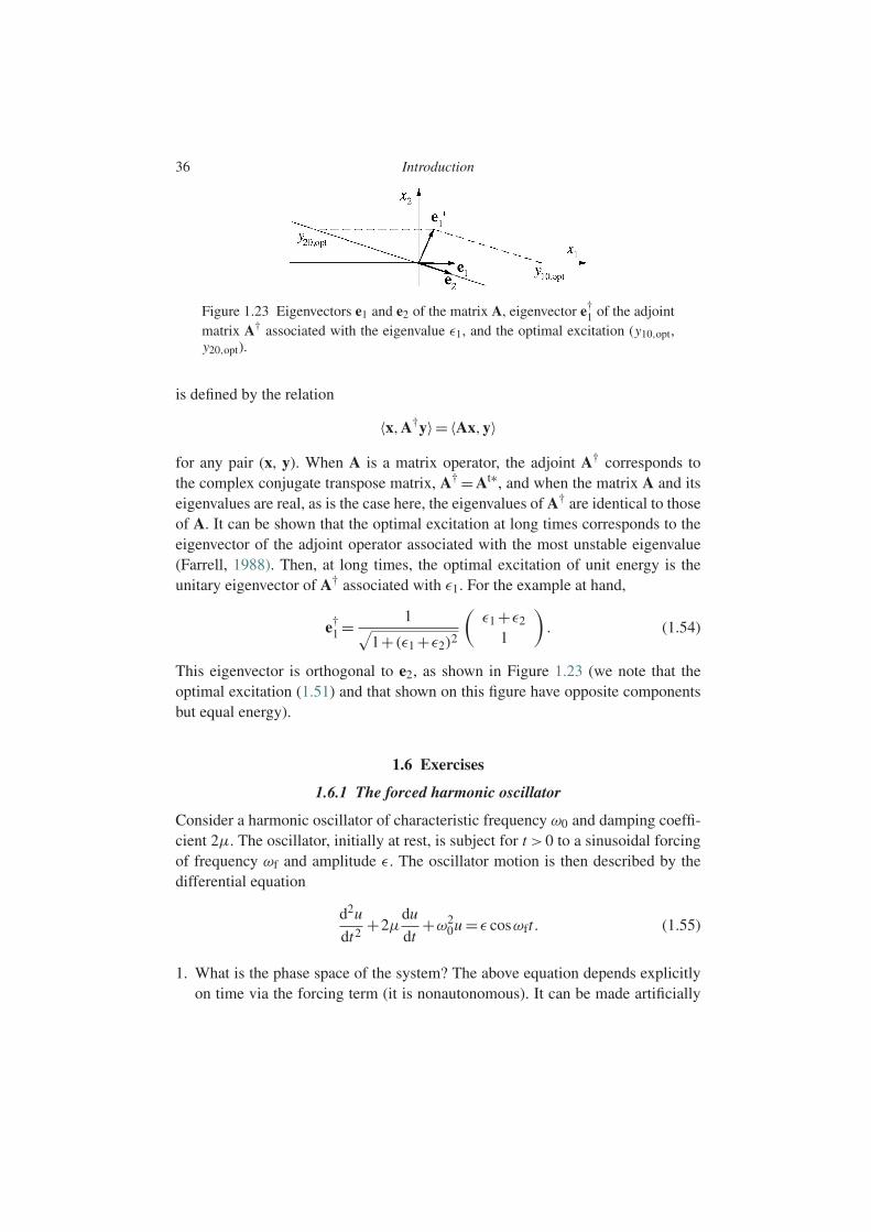
36 Introduction

Figure 1.23 Eigenvectors e1 and e2 of the matrix A, eigenvector e†1 of the adjoint

matrix A† associated with the eigenvalue ε1, and the optimal excitation (y10,opt,y20,opt).

is defined by the relation

〈x,A†y〉= 〈Ax,y〉for any pair (x, y). When A is a matrix operator, the adjoint A† corresponds tothe complex conjugate transpose matrix, A† =At∗, and when the matrix A and itseigenvalues are real, as is the case here, the eigenvalues of A† are identical to thoseof A. It can be shown that the optimal excitation at long times corresponds to theeigenvector of the adjoint operator associated with the most unstable eigenvalue(Farrell, 1988). Then, at long times, the optimal excitation of unit energy is theunitary eigenvector of A† associated with ε1. For the example at hand,

e†1 = 1√

1+(ε1 +ε2)2

(ε1 +ε2

1

). (1.54)

This eigenvector is orthogonal to e2, as shown in Figure 1.23 (we note that theoptimal excitation (1.51) and that shown on this figure have opposite componentsbut equal energy).

1.6 Exercises

1.6.1 The forced harmonic oscillator

Consider a harmonic oscillator of characteristic frequency ω0 and damping coeffi-cient 2µ. The oscillator, initially at rest, is subject for t >0 to a sinusoidal forcingof frequency ωf and amplitude ε. The oscillator motion is then described by thedifferential equation

d2u

dt2+2µ

du

dt+ω2

0u = ε cosωft. (1.55)

1. What is the phase space of the system? The above equation depends explicitlyon time via the forcing term (it is nonautonomous). It can be made artificially

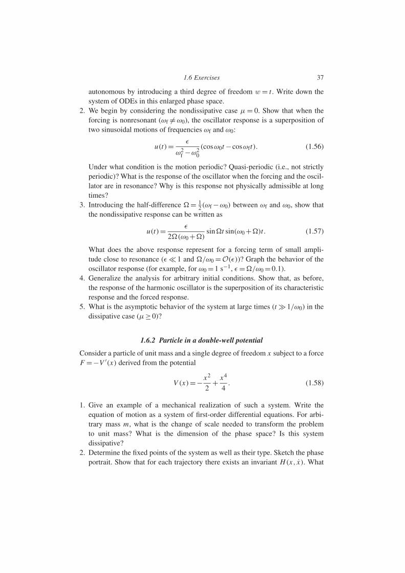
1.6 Exercises 37

autonomous by introducing a third degree of freedom w = t . Write down thesystem of ODEs in this enlarged phase space.

2. We begin by considering the nondissipative case µ = 0. Show that when theforcing is nonresonant (ωf =ω0), the oscillator response is a superposition oftwo sinusoidal motions of frequencies ωf and ω0:

u(t)= ε

ω2f −ω2

0

(cosω0t −cosωft). (1.56)

Under what condition is the motion periodic? Quasi-periodic (i.e., not strictlyperiodic)? What is the response of the oscillator when the forcing and the oscil-lator are in resonance? Why is this response not physically admissible at longtimes?

3. Introducing the half-difference = 12(ωf −ω0) between ωf and ω0, show that

the nondissipative response can be written as

u(t)= ε

2(ω0 +)sint sin(ω0 +)t. (1.57)

What does the above response represent for a forcing term of small ampli-tude close to resonance (ε 1 and /ω0 =O(ε))? Graph the behavior of theoscillator response (for example, for ω0 =1 s−1, ε =/ω0 =0.1).

4. Generalize the analysis for arbitrary initial conditions. Show that, as before,the response of the harmonic oscillator is the superposition of its characteristicresponse and the forced response.

5. What is the asymptotic behavior of the system at large times (t 1/ω0) in thedissipative case (µ≥0)?

1.6.2 Particle in a double-well potential

Consider a particle of unit mass and a single degree of freedom x subject to a forceF =−V ′(x) derived from the potential

V (x)=− x2

2+ x4

4. (1.58)

1. Give an example of a mechanical realization of such a system. Write theequation of motion as a system of first-order differential equations. For arbi-trary mass m, what is the change of scale needed to transform the problemto unit mass? What is the dimension of the phase space? Is this systemdissipative?

2. Determine the fixed points of the system as well as their type. Sketch the phaseportrait. Show that for each trajectory there exists an invariant H(x, x). What

38 Introduction

does this invariant represent physically? Derive the equation for the trajecto-ries and complete the phase portrait. Interpret these trajectories in terms of theparticle motion.

3. Without any calculation, but instead imagining a ball in a double-well potential,show how a friction force −µx (µ>0) modifies the type of fixed point. Sketchthe phase portrait.

4. Answer the above questions for the potential W (x) = −V (x). For additionaldiscussion, see Guckenheimer and Holmes (1983, §2.2).

1.6.3 Avalanches in a sand pile

Consider the nonlinear oscillator

ψ −γ ψ2 +kψ =0, γ ≥0, k real, (1.59)

which can be interpreted as an oscillator with a friction term (ψ)ψ involvinga nonconstant friction coefficient (ψ)= −γ ψ . This oscillator is a rudimentarymodel of avalanches in a sand pile, with ψ representing the deviation of theslope of the sand pile from the equilibrium slope; see Linz (1995). An avalanchecorresponds to ψ <0, and ψ =0 corresponds to the stopping of the avalanche.

1. Write Eq. (1.59) as a system of two first-order ODEs, and study the lin-ear stability of the fixed point as a function of the value of k. What can weconclude?

2. Equation (1.59) can be written as

d

dt

(ψ e−γψ

)= F(ψ), F(ψ)=−kψ e−γψ, (1.60)

which can be interpreted as the equation of motion of a mass e−γψ dependingon the position ψ and subject to a force F(ψ). We then define the kinetic energyEk and the potential V of the system as

Ek = 1

2e−2γψψ2, V =− k

4γ 2(1+2γψ)e−2γψ . (1.61)

Show that the extrema of V are the equilibrium positions (F = 0), the min-ima and maxima respectively corresponding to stable and unstable equilibriumstates. Verify that the energy Ek +V of the system remains constant throughoutthe motion.

3. Study the variations of the potential V in the cases k < 0 and k > 0. Sketch thebehavior of the potential V as a function of γψ for k = −4γ 2 and k = 4γ 2.Find the equilibrium positions of the system and their stability. Compare theseresults with those of the first question.

1.6 Exercises 39

4. For what values of k and the energy does the system (1.59) possess periodicsolutions?

5. Sketch the phase portrait of the system (1.59) for k <0 and k >0 with referenceto the behavior of the potential V .

1.6.4 A second-order phase transition

Consider a pure material near a phase transition. The thermodynamic state of thematerial is described by an “order parameter” A(t) assumed to be uniform in space(since the material is homogeneous). This order parameter might be the molarvolume of a fluid, the magnetization of a ferromagnetic material, the orientation ofliquid crystals, and so on. The order parameter obeys the real equation

dA

dt=−V ′(A), V (A)=µ

A2

2−α

A4

4− A6

6, (1.62)

where V ′(A) is the derivative of the thermodynamic potential V (A). This equationexpresses the fact that the rate of variation of the order parameter is proportional tothe slope of the thermodynamic potential V (A). Here, µ is the control parameterof the transition proportional to the difference from the transition temperature. Inthis exercise we take α=1.

1. Show that the stable and unstable fixed points respectively correspond to theminima and maxima of V (A). Justify the term thermodynamic potential for thefunction V (A).

2. Sketch the behavior of the potential as a function of the control parameter µ

and find the bifurcation diagram as a function of µ. Specify the nature of thebifurcation.

1.6.5 A first-order phase transition

For the same situation as in the preceding exercise we now take α = −1 in theexpression for the potential (1.62). The order parameter can take only positive orzero values. To make the ideas more precise, suppose that A=0 represents a liquidphase and A>0 a solid phase of the pure material.

1. Show that outside an interval [µ1,µ2], to be determined, the potential has asingle minimum, while inside this interval it has two minima which are equalfor a value µ0 to be calculated. Graph the potential in the two cases.

2. Sketch the bifurcation diagram as a function of the control parameter µ. Specifythe nature of the displayed bifurcations in µ=µ1 for µ decreasing from µ0,and in µ = µ2 for µ increasing from µ 0. Are µ1 and µ2 equal? What is

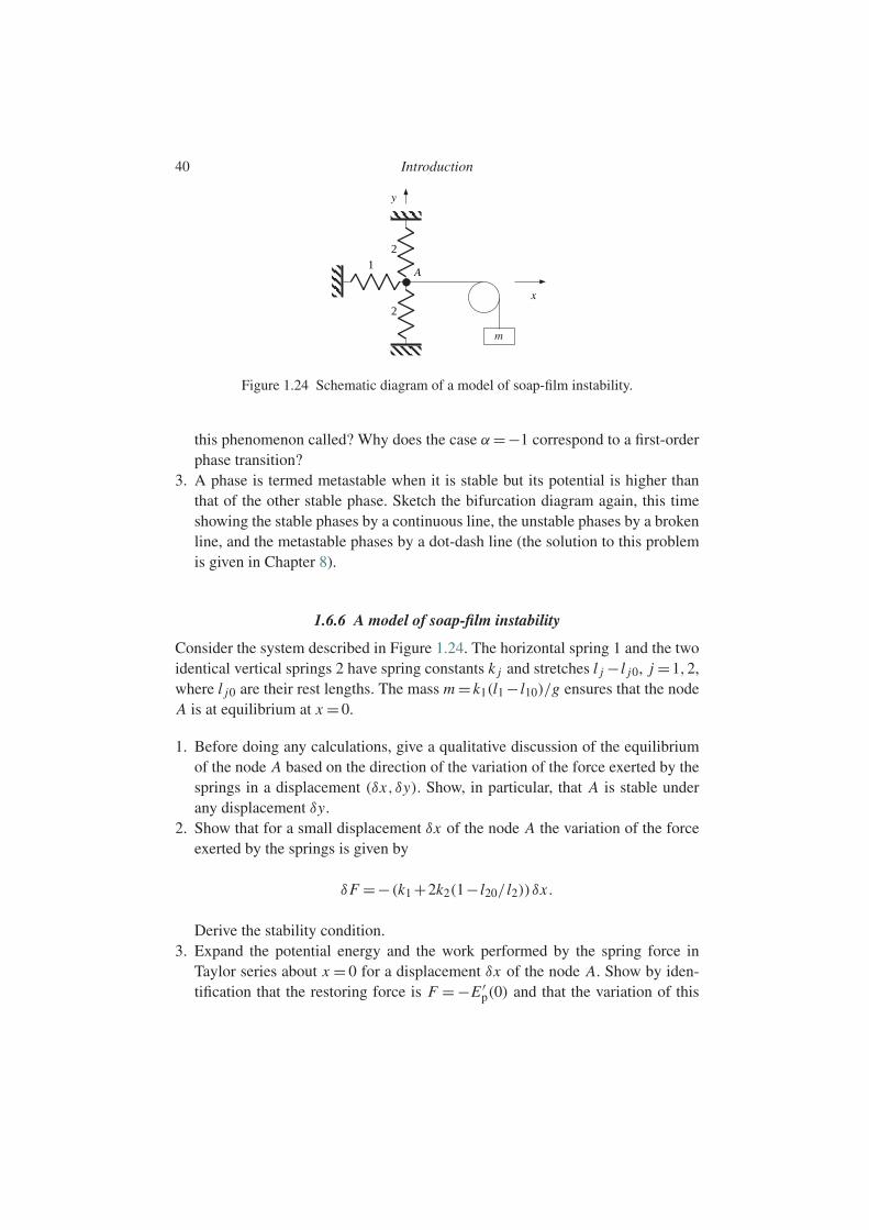
40 Introduction

y

x

m

12

2

A

Figure 1.24 Schematic diagram of a model of soap-film instability.

this phenomenon called? Why does the case α=−1 correspond to a first-orderphase transition?

3. A phase is termed metastable when it is stable but its potential is higher thanthat of the other stable phase. Sketch the bifurcation diagram again, this timeshowing the stable phases by a continuous line, the unstable phases by a brokenline, and the metastable phases by a dot-dash line (the solution to this problemis given in Chapter 8).

1.6.6 A model of soap-film instability

Consider the system described in Figure 1.24. The horizontal spring 1 and the twoidentical vertical springs 2 have spring constants k j and stretches l j −l j0, j =1,2,where l j0 are their rest lengths. The mass m = k1(l1 − l10)/g ensures that the nodeA is at equilibrium at x =0.

1. Before doing any calculations, give a qualitative discussion of the equilibriumof the node A based on the direction of the variation of the force exerted by thesprings in a displacement (δx,δy). Show, in particular, that A is stable underany displacement δy.

2. Show that for a small displacement δx of the node A the variation of the forceexerted by the springs is given by

δF =−(k1 +2k2(1− l20/ l2))δx .

Derive the stability condition.3. Expand the potential energy and the work performed by the spring force in

Taylor series about x = 0 for a displacement δx of the node A. Show by iden-tification that the restoring force is F = −E ′

p(0) and that the variation of this

1.6 Exercises 41

force is δF =−E ′′p (0)δx . Derive the stability condition in terms of the convex-

ity of the potential energy of the springs. What is the potential (different thanthe potential energy Ep) whose extrema correspond to the equilibrium states?

1.6.7 Transient growth and optimal perturbation

Derive the results (1.43) to (1.47) for the system (1.42).

1.6.8 Optimal excitation of an unstable mode

Consider the dynamical system (1.48),

dxdt

=Ax, A=(

ε1 10 −ε2

),

where ε1 and ε2 are two small positive parameters associated with the initialcondition x0 = (x10, x20).

1. Show that the eigenvalues of the system are ε1 and −ε2, respectively associatedwith the unitary eigenvectors (1.49).

2. We define the energy of the system at time t as E(t)=x(t) ·x(t). Owing to thelinear nature of the problem, without loss of generality we can consider the caseof unit initial energy E0 =x(0) ·x(0)=1, with x(0)= y10e1 + y20e2. Show thatthe energy E(t) can be written as

E(t)/e2ε1t −1

1−α= (2p2 −1−α)y2

20 ±2p y20

√1−(1− p2)y2

20 ,

where α= e−(ε1+ε2)t and p = e1 ·e2.3. Show that the initial conditions y20 which make the energy E an extremum at

time t are the roots of the biquadratic equation

(1− p2)y420 − y2

20 + p2

4p2(1− p2)+(1−α−2(1− p2))2=0.

4. Using the linearity of the system of differential equations, without loss of gen-erality we can seek only the positive roots. Show that for ε1 1 and ε2 1 andusing 1− p2 ∼ (ε1 +ε2)

2, the positive roots of the above equation are

y(1)20 = 1

1−α+O(ε1 +ε2), y(2)

20 = 1

ε1 +ε2+O(1).

Find the corresponding initial conditions y(1)10 and y(2)

10 .

42 Introduction

5. Show that the optimal gain (1.52) corresponds to the initial condition y(2)20 , and

that at long times (ε1t 1 and ε2t 1) this gain is given by (1.53). Qualitativelysketch ln(E(t)/E0) as a function of time for initial condition corresponding to(a) the energy at the single unstable mode, and (b) the energy at the optimalexcitation. What do you conclude?

6. Discuss the meaning of the initial condition y(1)20 .

1.6.9 Subcritical bifurcation via a transient growth

Construct a nonlinear dynamical system with two degrees of freedom which has afixed point displaying subcritical pitchfork bifurcation for a critical value µc of aparameter µ, and such that for µ<µc there exist unstable initial conditions owingto a transient growth. It may be helpful to consult Trefethen et al. (1993).

2

Instabilities of fluids at rest

2.1 Introduction

In this chapter we discuss how various gravitational, capillary, and thermal phe-nomena can initiate an instability in a fluid initially at rest. In such a motionlessfluid, advection of momentum plays a negligible role in the small amplitude the-ory, unlike the situations that will be studied in later chapters. We also present thebasic techniques for studying linear stability: derivation of the equations for smallperturbations of a base state, linearization, and determination of the normal modesand the dispersion relation.

An important part of this chapter is devoted to the analysis of problems in termsof ratios of characteristic scales. The approach we take is to simplify the problemby evaluating the order of magnitude of the involved phenomena before embark-ing on long analytic or numerical calculations. This allows us to retain only themost important effects and to elucidate mechanisms. This dimensional analysis,which is essential in both fundamental and applied research, is often sufficient fordetermining the scaling laws governing the problem. It allows the choice of a setof suitable reference scales to recast the problem in dimensionless form, or, inother words, to recast the problem in a system of units composed of scales thatare intrinsic to the problem. This modeling approach then guides the later calcula-tions, for example, by revealing a small parameter which suggests an asymptoticexpansion. It also serves to justify or reject a posteriori certain hypotheses, andleads to a better understanding of the physics of the problem.

This chapter is organized as follows. First we present the basic technique forstudying stability using the example of the gravitational instability of a cloud ofinterstellar gas (Section 2.2). We then study some classical instabilities related togravity, surface tension, and temperature gradients (Sections 2.3–2.6). From theseexamples we can abstract (Section 2.7) some common and fundamental featuresof broader generality introduced in the preceding chapter, such as the concepts

43

44 Instabilities of fluids at rest

of control parameter of an instability, bifurcation, symmetry breaking, and themechanism of structure selection.

2.2 The Jeans gravitational instability

The instability of a distribution of masses interacting gravitationally – an instabil-ity which should cause the Universe to collapse toward its center – did not escapethe notice of Isaac Newton. After speculating with the theologian Richard Bentleyabout what he considered to be an unacceptable collapse, Newton concluded in1692 that our Universe must be infinite, as then it has no center, and therefore nocollapse: “...providence had designed a Universe of infinite extent in which uni-formly distributed stars stand poised in unstable equilibrium like needles on theirpoints” (Edward Harrison; quoted by Longair, 2006). In 1902 the British physicistSir James Jeans made a major advance in solving this problem by determining alength scale above which a mass of uniformly distributed gas is effectively unsta-ble. The problems that this study raised led to much later research, which continuestoday, to better understand the formation and evolution of stars, galaxies, and theUniverse. Here we give an elementary introduction to the subject. First we dis-cuss the effect of terrestrial gravity on classical acoustic waves, which allows usto introduce the fundamental ideas of normal modes and a dispersion relation. Wethen turn to the case of a nonuniform gravitational field within the framework ofthe Jeans approximation. Finally, we briefly discuss this approximation in the lightof some recent developments.

2.2.1 Acoustic waves

Base state, perturbations, and linearization

Let us consider a fluid – a liquid or a gas – at rest in the Earth’s gravitational fieldg. The velocity, density, and pressure fields are defined as

U=0, ρ =ρ0, P = P0 −ρ0gz, (2.1)

where ρ0 and P0 are the density and pressure at a reference altitude z = 0. Thesequantities define a base state satisfying the laws of mass and momentum conser-vation (at least on a height scale for which the density variation associated withfluid compressibility can be neglected. As an example, for a height variation ofone hundred meters, the density variation of the Earth’s atmosphere is 1.7% andthat of the ocean, 0.04%).

Under a small perturbation of this base state, the velocity, density, and pressurefields become

U=U+u, ρ =ρ+ρ′, P = P + p.

2.2 The Jeans gravitational instability 45

The evolution of these fields must satisfy the laws of mass and momentumconservation:

∂tρ+div(ρU)=0, (2.2a)

ρ(∂t U+(U·grad)U)=−gradP +ρg. (2.2b)

It can be verified a posteriori that the viscosity effects omitted above are negligible;we have, however, included gravity, which is essential to our discussion. A fifthequation is necessary to account for the thermodynamic behavior of the fluid andto close the system of equations. Assuming the evolution of the perturbations tobe isentropic (adiabatic and reversible), the variations of the density and pressureperturbations are related via the equation of state:

dρ = ∂ρ

∂P

∣∣∣∣s

dP =ρκs dP, (2.3)

where κs is the isentropic compressibility (Callen, 1985). Taking into account theequation of hydrostatic equilibrium satisfied by the base state,

0=−grad P +ρg,

and linearizing the above equations about this base state neglecting products ofperturbations, we obtain

∂tρ′ +ρ0 divu=0, (2.4a)

ρ0∂t u=−grad p+ρ′g, (2.4b)

ρ′ =ρ0κs p. (2.4c)

Taking the divergence of (2.4b) and substituting Eqs (2.4a) and (2.4c) results in anequation involving only the pressure:

∂2t p−c2

sp+g ·grad p =0, (2.5)

where we have introduced the speed cs defined as

cs = 1√ρ0κs

. (2.6)

We note that for g = 0 we recover the classical equation for acoustic waves(Lighthill, 1978; Billingham and King, 2000).

Normal modes and the dispersion relation

Equation (2.5) above is linear with constant coefficients (a reflection of the trans-lation invariance of the problem), and therefore for unbounded domains admits

46 Instabilities of fluids at rest

solutions that are exponentials in time and in space. These solutions can bewritten as

p = 1

2p ei(k·r−ωt)+c.c., (2.7)

where c.c. stands for complex conjugate, corresponding to plane waves of wavevector k and angular frequency ω, with amplitude p. This amplitude, which isa priori complex, can be written as | p|eiθ where | p| and θ are its modulus andphase.1 For k real and ω=ωr + iωi complex, the perturbation can be written as

p =| p|eωit cos(k·r−ωrt +θ)

(in the next chapter we shall consider the more general situation of complex wavenumber). The real part of the angular frequency ωr therefore corresponds to prop-agation of the perturbation at speed c=ωr/k, where k =|k|. The imaginary part ωi

is the temporal growth rate: ωi <0 corresponds to a damped perturbation, ωi =0 toa neutral perturbation, and ωi > 0 to an amplified perturbation. Any perturbation,like a localized excitation, can be treated as a superposition of perturbations ofthe form (2.7) which, in a linearized problem, evolve independently of each other.Such perturbations are called the normal modes (owing to the orthogonality ofthe exponential functions). Thus, when studying linear stability, we can in generalconsider only the evolution of a single generic normal mode of the form (2.7); thisstatement will be made more precise in the next chapter.

With (2.7) the wave equation (2.5) becomes

−ω2 p+c2s k2 p+ ig·k p =0.

This equation has a nonzero solution only if the coefficient of p is zero, i.e.

ω2 = c2s k2 + ig·k. (2.8)

This is the dispersion relation for small perturbations; it shows that the frequencyand the wave vector of a normal mode, or eigenmode, are not independent, but arerelated in a specific way. The dispersion relation does not involve the amplitudeof the perturbation, which remains undetermined owing to the linear and homoge-neous nature of Eq. (2.5). Here we have managed to solve the system (2.4) simplyby substitution; as we shall see in the following section, the introduction of normalmodes leads more generally to a homogeneous algebraic system for the amplitudesof the perturbations, which has a nonzero solution only if its determinant vanishes;it is this more general condition that gives the dispersion relation.

1 The coefficient 1/2 in (2.7) may be omitted since the problem to be solved is linear and homogeneous; however,it is introduced for consistency with the nonlinear analyses of later chapters.

2.2 The Jeans gravitational instability 47

Temporarily ignoring the last term ig·k in the dispersion relation, we see thatthe frequency of a wave with real wave vector is ω=±csk; it is real, which cor-responds to a wave which propagates without amplification or attenuation. Thephase velocity of this wave, also called the wave speed, is

c = ω

k=±cs, (2.9)

which explains the physical meaning of the speed cs. We note that this speed, the“speed of sound,” is independent of the wave number, i.e., acoustic waves are notdispersive. In air (assumed to be an ideal gas), we find2 cs =√

γ rT0 = 340 m s−1

for T0 = 288 K; therefore, a typical acoustic wave of frequency ω/2π = 1000 Hzhas wavelength λ = 2π/(ω/cs) = 0.34 m. In water, which has compressibilityκs ≈0.47×10−9 Pa−1, the speed of sound is cs ≈1460 m s−1, and the wavelengthat the same frequency is λ = 1.46 m. Let us now consider the effect of gravity,which corresponds to the term ig·k. The first thing to note is that this effectarises only when the wave vector has a vertical component. For audible acous-tic waves of wavelength about a meter, the order of magnitude of the gravity termcompared to ω2 is 10−5, so that the effect of gravity is completely negligible.But gravity does become important for waves of frequency below 1 Hz, whosewavelength is about a kilometer. However, for such long waves the assumption ofuniform gravitational field must be revised. This is the subject of the followingsection.

2.2.2 The effect of gravity at large scales

Dimensional analysis

As shown in the preceding section, the propagation of an acoustic wave with speedcs is essentially a consequence of a balance between the fluid inertia and an elasticrestoring force due to the fluid compressibility. Gravity plays a role only at lengthscales above c2

s /g, which is about 10 km for the Earth’s atmosphere and 200 km forthe ocean. Thus the role of gravity is essential at the scale of astrophysical phenom-ena. In particular, it gives rise to an instability of an interstellar gas cloud whichcauses the cloud to collapse on itself, leading to star formation. This instability canbe analyzed qualitatively as follows.

First we recall that a mass m produces a gravitational field G = Gm/r2 at adistance r , where G = 6.67 × 10−11 m3/kg/s2 is the gravitational constant, and

2 The isentropic compressibility of an ideal gas is κs =γ /P , where γ = cp/cv is the adiabatic index (the ratio ofthe heat capacity at constant pressure to the heat capacity at constant volume). Taking into account the Boyle–Mariotte law P/ρ = rT , where r = R/M is the ratio of the ideal gas constant R = 8.314 J K−1 mol−1 and themolar mass M , one obtains c2

s =γ rT0. For air, γ =1.4 and M =29.0 g mol−1.

48 Instabilities of fluids at rest

that this gravitational field exerts on a mass m′ an attractive force m′G. Now letus take a large mass of gas at rest, for example, an interstellar gas cloud, andperturb its equilibrium by density and pressure nonuniformities δρ and δP on aspatial scale L . This leads to a nonuniformity of the gravitational field of orderδG ∼ G δρL3/L2 = G δρL . A fluid particle of typical size a is then subject totwo competing forces, an elastic force and a gravitational force. The elastic force,which is related to the compressibility of the fluid, points from compressed regionsto neighboring rarefied regions, and its order of magnitude is

Fa ∼ (δP/L)a3 ∼ δρ c2s a3/L .

The net gravitational force is directed toward the compressed region containing amass excess of order δρL3, and its order of magnitude is

Fg ∼ρa3 δG∼ρa3 G δρ L .

The ratio of these two forces is then Fg/Fa =ρGL2/c2s . Thus, if the spatial scale of

the nonuniformities is such that L cs/√ρG, the elastic force dominates and the

perturbation propagates as an acoustic wave, without amplification. Conversely, ifL cs/

√ρG, the gravitational force dominates and the gas moves from rarefied

regions to compressed ones, which enhances the initial density difference. Thus,the effect amplifies the cause, and an instability develops which destroys the initialuniformity of the cloud and causes it to collapse.3

The dimensional analysis carried out above therefore indicates a length scale

Lc = cs√ρG

(2.10)

above which a mass of gas is susceptible to collapsing on itself. This length cor-responds (up to a numerical factor) to the length discovered by Jeans in 1902.For the Earth’s atmosphere this length is about 36,000 km, which is much largerthan the Earth’s radius: gravity does not enter into the propagation of soundwaves, and so the Earth’s atmosphere is not at risk of collapse! For a low-densitycloud of interstellar gas, where the parameters are typically cs = 200 m s−1 andρ=2×10−17 kg m−3, the length Lc is about 5×1012 km, that is, about a thousandtimes the size of the Solar System, or half a light-year.4

3 The analogy with a liquid–vapor phase transition should be noted: the liquid results from “collapse” of the gas.However, in this case it is not the gravitational interaction which is responsible for the instability, but ratherinteractions of the van der Waals type.

4 This analysis is incorrect for astrophysical objects which are very dense such as white dwarfs, whose densityis of order 5×106 g/cm. For such objects it is a pressure of quantum rather than thermal origin which opposesthe gravitational attraction and ensures equilibrium.

2.2 The Jeans gravitational instability 49

The base state, perturbations, and linearization

We now make the above dimensional analysis quantitative by considering solutionsto the linearized equations. Consider a large cloud of interstellar gas of density ρ,pressure P , and temperature T , assumed to be an ideal gas (Chandrasekhar, 1961,§119). The stability of this cloud can be studied from the thermodynamic point ofview by seeking the extrema of a suitable thermodynamic potential (the entropy foran isolated system described by the microcanonical formalism, or the free energyfor a system held at constant temperature and described by the canonical formalism(Chavanis, 2002)). Equivalently, this stability can be studied using the mechanicsof continuous media. It is this latter approach that we follow here. The conserva-tion equations are then identical to Eqs (2.2) governing acoustic waves, with thegravitational acceleration g replaced by the gravitational field G=−grad, where is the gravitational potential:

∂tρ+divρU=0, (2.11a)

ρ(∂t U+(U·grad)U)=−gradP −ρ grad. (2.11b)

The gravitational potential is related to the density distribution by the Poissonequation:

=4πGρ. (2.12)

Finally, as before, we assume that the perturbations evolve isentropically, with theentropy given by the equation of state (Callen, 1985):

s −s0 = cv lnP

P0−cp ln

ρ

ρ0, (2.13)

where cv and cp are the heat capacities at constant volume and pressure, and thesubscript 0 refers to a reference equilibrium state.

We note first of all that equations (2.11)–(2.12) do not admit a solution withuniform P and ρ: for such a solution, the potential would have to be uniformaccording to (2.11b), and the Poisson equation (2.12) would then imply ρ = 0. Anonuniform hydrostatic equilibrium can be found for a spherical mass distribu-tion, corresponding to a uniform temperature and a density which varies as 1/r2,where r is the distance to the center of the distribution (Binney and Tremaine,1988). However, this distribution corresponds to infinite total mass (the mass∫ρ(r)4πr2dr in a sphere of radius R diverges as R). This difficulty can be over-

come by artificially confining the gas inside a sphere of radius R (Chavanis, 2002).A full treatment of this problem lies outside the scope of the present book, and sohere we shall consider the simplified version studied by Jeans in 1902. The sim-plification is to study the stability of a uniform base state, although this base state

50 Instabilities of fluids at rest

does not satisfy the Poisson equation (2.12). In spite of this simplification, knownas the “Jeans swindle” (Binney and Tremaine, 1988), the calculation merits repro-duction owing to its historical importance and the fact that in the end it gives astability condition close to that obtained in the solution of the full problem.5

Let us consider a stationary and uniform base state defined as

U=0, ρ =ρ0, s = s0, =0, P = P0, (2.14)

and a small isentropic perturbation of this base state, u, ρ′, φ, and p. The equationsgoverning the evolution of these perturbations are then, according to (2.11)–(2.13),

∂t (ρ0 +ρ′)+div((ρ0 +ρ′)u

)=0, (2.15a)

(ρ0 +ρ′)(∂t u+(u·grad)u)=−grad(P0 + p)−(ρ0 +ρ′)grad(0 +φ),

(2.15b)

φ=4πGρ′, (2.15c)

ln(1+ p

P0)−γ ln(1+ ρ′

ρ0)=0. (2.15d)

We note that, although the base state does not satisfy the Poisson equation, theperturbations do. For small perturbations we can linearize the equations about thebase state neglecting products of perturbations. The linearized equations are then

∂tρ′ +ρ0 divu=0, (2.16a)

ρ0 ∂t u=−gradp−ρ0 gradφ, (2.16b)

φ=4πGρ′, (2.16c)

p = c2sρ

′. (2.16d)

Normal modes and the dispersion relation

Like the problem of acoustic waves treated above, the problem (2.16) is linear withconstant coefficients, again a reflection of its translation invariance. It thereforehas solutions which are exponentials in time and space and can be written as planewaves of wave vector k and frequency ω:

u = 1

2u ei(k·r−ωt)+c.c., (2.17)

with similar expressions for the other velocity components v and w, as well as forρ′, p, and φ.

5 The “Jeans swindle” in fact becomes legitimate in cosmology when the expansion of the Universe is taken intoaccount, in which case the Poisson equation is involved only for the perturbations.

2.2 The Jeans gravitational instability 51

Taking the divergence of (2.16b), by substitution we obtain an equationinvolving only the pressure perturbation p:

∂2t p−c2

sp−4πρ0G p =0. (2.18)

For a normal mode of the form (2.17) this equation becomes

ω2 p = c2s k2 p−4πGρ0 p, (2.19)

where k =|k|. This equation has a nonzero solution only when the coefficient of pvanishes, from which we find the dispersion relation:

ω2 = c2s k2 −4πGρ0. (2.20)

Note that this is the dispersion relation (2.8) for acoustic waves with the correctedgravitational term 4πGρ0.

2.2.3 Discussion

Let us now study the dispersion relation (2.20) by considering a plane wavewith real wave vector k whose temporal stability is to be determined. Since thedispersion relation is quadratic in ω, there exist two eigenmodes with frequency

ω±(k)=±√

c2s k2 −4πGρ0.

This indicates the existence of a critical wave number

kJ =√

4πGρ0

cs(2.21)

for which the expression in the square root vanishes. Any perturbation with wavenumber above kJ has real frequency, and therefore corresponds to a wave whichpropagates without growth or decay with velocity

c± =ω±/k =±cs

√1−k2

J /k2 (k > kJ),

which is close to cs for short wavelengths (k kJ) and vanishes at k = kJ. On theother hand, any perturbation with wave number below kJ has purely imaginaryfrequency. The mode corresponding to ω+ =+iωi grows exponentially at a rate

ωi = cs

√k2

J −k2 (k < kJ),

while the other mode of frequency ω− =−iωi decreases exponentially. The phasevelocity of these modes, c =ωr/k, is zero.

52 Instabilities of fluids at rest

We conclude that in a gas cloud of size smaller than the Jeans length LJ =2π/kJ,any perturbation propagates without amplification, and so the cloud is linearlystable. On the other hand, if the cloud is larger than the Jeans length, it is unstablewith respect to perturbations of large wavelength. We note that LJ corresponds,up to a numerical factor

√π , to the critical length (2.10) obtained in our earlier

dimensional analysis.

Subrahmanyan Chandrasekhar (1910–1995)

Subrahmanyan Chandrasekhar was born inLahore, India (now Pakistan) into a well-off, cultivated Brahmin family. One of hisuncles, Sir Chandrasekhara Venkata Raman,was awarded the Nobel Prize in Physics in1930 for his discovery of the optical effectbearing his name. He did his secondary andundergraduate studies in Madras, at whichtime he published his first article in the Pro-ceedings of the Royal Society. Following theexample of his uncle, he left India in 1930 tostudy at Trinity College, Cambridge, England,where he obtained his doctorate in 1933. He

got married in India in 1936, and then moved to the University of Chicagowhere he remained for the rest of his life. During World War II he worked onshock waves and detonation. He was elected a Fellow of the Royal Society ofLondon in 1944. He and his wife became American citizens in 1953. He con-tributed to many fields in physics, including white dwarfs, stellar dynamics,radiation, hydrodynamic and hydromagnetic stability, general relativity, blackholes, and gravitational waves. In particular, he showed that a star of mass lessthan 1.44 solar masses evolves at the end of its life into a white dwarf, whilea star of mass greater than this limit collapses violently into an object of enor-mous density, a neutron star or a black hole. He won the Nobel Prize in 1983for his work on stellar structure and evolution. He published about 400 papersand many important books, in particular, Hydrodynamic and HydromagneticStability (1961). He received many honors, including the Royal Medal (1962)and the Copley Medal (1984) of the Royal Society of London. He was edi-tor in chief of the Astrophysical Journal for 19 years, and raised its statureenormously. He was interested in the connections between art and science, andlater in life wrote the books Truth and Beauty: Aesthetics and Motivations inScience (1987) and Newton’s Principia for the Common Reader (1995), and

2.3 The Rayleigh–Taylor interface instability 53

gave thought-provoking lectures such as Shakespeare, Newton and Beethovenor patterns of creativity and one on comparison of Newton’s Principia andMichelangelo’s frescoes in the Sistine Chapel.

Let us now return to the “Jeans swindle” for the case of a uniform basestate. This swindle can be considered acceptable on a length scale over whichthe gravitational potential is nearly constant, i.e. the scale given by the Poissonequation. Actually, since the equilibrium condition imposes ρ/L ∼ P/L withP/ρ = c2

s /γ ≈ c2s , the Poisson equation gives

c2s

L2∼

L2∼4πGρ.

The length scale L that appears is again none other than the critical length (2.10)(up to a numerical factor of order unity)! Therefore, the conclusion that a cloudof uniform density and size smaller than LJ is stable appears completely reason-able for a realistic cloud of nonuniform density satisfying the Poisson equation.The appearance of an instability for a cloud of size of order LJ suggested by thedimensional analysis also seems quite plausible. On the other hand, the result ofmaximal growth rate for k = 0 is not reasonable. Recent studies on this subjectconfirm these conclusions (Chavanis, 2002). Interestingly, a study of the nonlinearevolution of the instability suggests a fractal organization of the mass distributionat the time of its collapse (de Vega et al., 1996).

2.3 The Rayleigh–Taylor interface instability

2.3.1 Dimensional analysis

We consider two infinitely deep superposed fluid layers subject to constant gravityand separated by a horizontal interface. We shall first neglect viscosity and assumethat the walls bounding the fluid are far enough from the interface to be ignored(the effect of walls and of viscous forces is studied in Exercises 2.8.1 and 2.8.2).The only physical variables then are the two densities ρ1 and ρ2, the surface tensionγ , and gravity g. These four dimensional variables bring in the three fundamentaldimensions of mass, length, and time, and so the problem depends on only a singledimensionless parameter, namely, the density contrast or the Atwood number,

At= ρ1 −ρ2

ρ1 +ρ2. (2.22)

This key parameter is negative if the denser fluid is on top, and positive in theopposite case. It is equal to 1.0 if the upper fluid has negligible density, as for thecase of a gas on top of a liquid, and equal to −1.0 in the opposite case of liquidover gas.

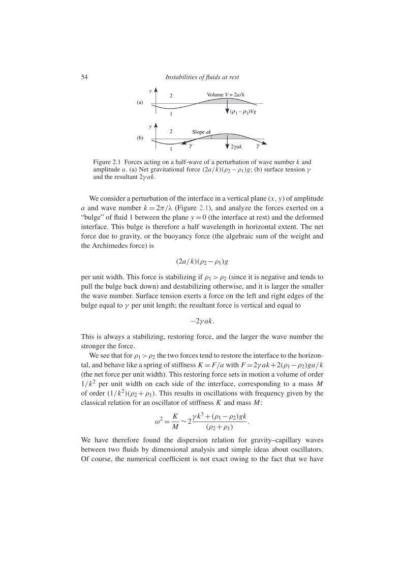
54 Instabilities of fluids at rest

2

2

(a)

(b)

1

1

Slope ak

Volume V = 2a/k

2γ ak

(ρ1 – ρ2)Vg

y

y

γ γ

Figure 2.1 Forces acting on a half-wave of a perturbation of wave number k andamplitude a. (a) Net gravitational force (2a/k)(ρ2 −ρ1)g; (b) surface tension γand the resultant 2γ ak.

We consider a perturbation of the interface in a vertical plane (x, y) of amplitudea and wave number k = 2π/λ (Figure 2.1), and analyze the forces exerted on a“bulge” of fluid 1 between the plane y =0 (the interface at rest) and the deformedinterface. This bulge is therefore a half wavelength in horizontal extent. The netforce due to gravity, or the buoyancy force (the algebraic sum of the weight andthe Archimedes force) is

(2a/k)(ρ2 −ρ1)g

per unit width. This force is stabilizing if ρ1 >ρ2 (since it is negative and tends topull the bulge back down) and destabilizing otherwise, and it is larger the smallerthe wave number. Surface tension exerts a force on the left and right edges of thebulge equal to γ per unit length; the resultant force is vertical and equal to

−2γ ak.

This is always a stabilizing, restoring force, and the larger the wave number thestronger the force.

We see that for ρ1>ρ2 the two forces tend to restore the interface to the horizon-tal, and behave like a spring of stiffness K = F/a with F =2γ ak+2(ρ1−ρ2)ga/k(the net force per unit width). This restoring force sets in motion a volume of order1/k2 per unit width on each side of the interface, corresponding to a mass Mof order (1/k2)(ρ2 +ρ1). This results in oscillations with frequency given by theclassical relation for an oscillator of stiffness K and mass M :

ω2 = K

M∼2

γ k3 +(ρ1 −ρ2)gk

(ρ2 +ρ1).

We have therefore found the dispersion relation for gravity–capillary wavesbetween two fluids by dimensional analysis and simple ideas about oscillators.Of course, the numerical coefficient is not exact owing to the fact that we have

2.3 The Rayleigh–Taylor interface instability 55

estimated the amount of mass in motion. Comparison with the exact dispersionrelation given below in (2.40) shows that the effective mass is equal to twice themass estimated here.

For ρ1 <ρ2, gravity is destabilizing, and its action overcomes that of the surfacetension if

2(ρ2 −ρ1)ag/k −2γ ak >0.

We deduce that the interface is unstable to perturbations of wave number lowerthan a cutoff kc defined as

kc = 1

lc, with lc =

√γ

g|ρ2 −ρ1| , (2.23)

where lc is the capillary length (Guyon et al., 2001). For a water–air interface(γ =70×10−3 N/m) the capillary length is lc =2.7 mm. In the absence of surfacetension (two miscible liquids or two gases, for example, cold air above a layer ofwarm air) all wave numbers are unstable.

Therefore, with or without surface tension, the configuration of a heavy fluid ontop of a light one is always unstable to long wavelength perturbations. However,if an interface is confined to a length scale smaller than the capillary length, itis stable. This explains why a narrow vertical tube can hold a column of liquidwithout emptying.

The time for the instability to grow, i.e., the time over which the amplitude ofthe perturbation changes significantly, is on the order of the only time scale in theproblem, the capillary time:

τc =√

lcg

=(

γ

|ρ1 −ρ2|g3

)1/4

. (2.24)

The assumption of negligible viscosity and infinite vertical extent of the liquidscan now be made more precise. The length scale of the problem being the capillarylength lc, the walls limiting the vertical extent of the fluids do not play a role if thethickness of the layers is large compared to lc. Additionally, viscous effects canbe neglected if during the characteristic time for the instability to grow, τc, themomentum has not diffused appreciably, i.e., it has diffused only a small distancecompared to lc. This condition can be written as

√ντc lc.

In other words, viscosity effects are negligible if the capillary Reynolds numberRecap = l2

c/τcν is large compared to unity. This condition is satisfied for a water–air interface for which Recap = 15. Let us now carry out a quantitative analysis ofthe problem.

56 Instabilities of fluids at rest

2.3.2 Perturbation equations

The base state and nature of the perturbations

Here the base state corresponds to the fluid at rest, a planar interface η(x, z, t), anda hydrostatic pressure distribution:

U j =0, η=0, P j (y)− P0 =−ρ j gy, j =1,2, (2.25)

where P0 is a reference pressure at the interface. This state satisfies the conserva-tion equations and the boundary conditions, as we shall verify later on. Perturbingthis base state, the velocity, pressure, and interface position are written

U j =U j +u j ,

Pj = P j + p j ,

η=η+η.

The stability problem can be solved without loss of generality by consideringan irrotational perturbation, for which

u j =gradφ j

where φ j is the velocity potential. As justification, let us consider the Helmholtzequation for the vorticity perturbations ω, linearized about the rest state of thefluid:

∂tω= νω.

In the absence of viscous diffusion, this equation reduces to ∂tω = 0 (Batchelor,1967). The velocity field associated with an initial vorticity distribution can there-fore be only a time-independent field, which cannot participate in the growth of aninstability.

The conservation equations

In order to simplify the algebra, we consider perturbations which are two-dimensional in a vertical plane (x, y). The incompressibility equation can thenbe written as

∂xxφ j +∂yyφ j =0, j =1,2. (2.27)

The momentum conservation is given by the Bernoulli equation (the first integralof the Euler equations):

ρ j∂tφ j + 1

2ρ j (gradφ j )

2 +(P j + p j )+ρ j gy = P0, j =1,2,

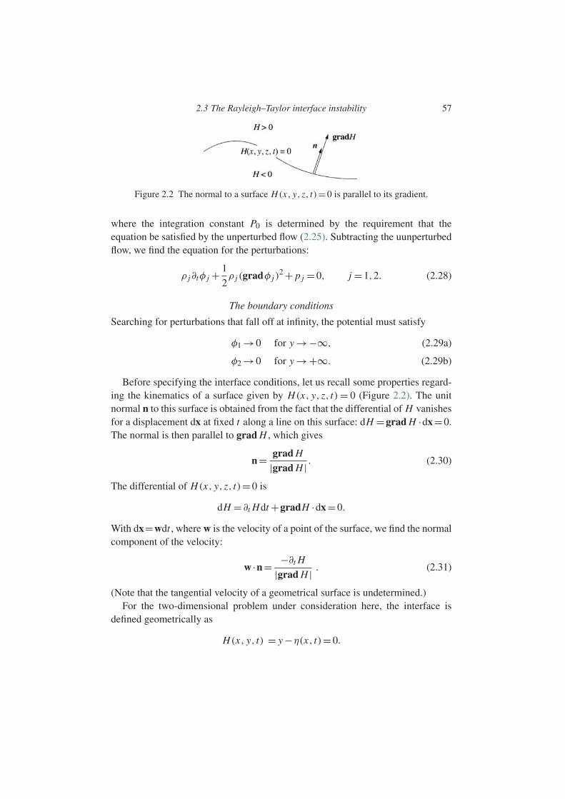
2.3 The Rayleigh–Taylor interface instability 57

Figure 2.2 The normal to a surface H(x, y, z, t)=0 is parallel to its gradient.

where the integration constant P0 is determined by the requirement that theequation be satisfied by the unperturbed flow (2.25). Subtracting the uunperturbedflow, we find the equation for the perturbations:

ρ j∂tφ j + 1

2ρ j (gradφ j )

2 + p j =0, j =1,2. (2.28)

The boundary conditions

Searching for perturbations that fall off at infinity, the potential must satisfy

φ1 →0 for y →−∞, (2.29a)

φ2 →0 for y →+∞. (2.29b)

Before specifying the interface conditions, let us recall some properties regard-ing the kinematics of a surface given by H(x, y, z, t)= 0 (Figure 2.2). The unitnormal n to this surface is obtained from the fact that the differential of H vanishesfor a displacement dx at fixed t along a line on this surface: dH =grad H ·dx=0.The normal is then parallel to grad H , which gives

n= grad H

|grad H | . (2.30)

The differential of H(x, y, z, t)=0 is

dH = ∂t Hdt +gradH ·dx=0.

With dx=wdt , where w is the velocity of a point of the surface, we find the normalcomponent of the velocity:

w ·n= −∂t H

|grad H | . (2.31)

(Note that the tangential velocity of a geometrical surface is undetermined.)For the two-dimensional problem under consideration here, the interface is

defined geometrically as

H(x, y, t) = y −η(x, t)=0.

58 Instabilities of fluids at rest

The normal and the normal velocity of the interface are then

n= (−∂xη,1)√1+∂2

xη, w ·n= ∂tη√

1+∂2xη

,

where ∂xη is the interface slope.There are two types of boundary condition at the interface: a “kinematic” con-

dition which expresses the impermeability of the interface, and a “dynamical”condition on the stresses. The kinematic condition states that in each fluid thenormal velocity at the interface U j ·n must be equal to the normal velocity w·n ofthe interface:

U j ·n=w·n at y =η(x, t), j =1,2,

or

∂xφ1 (−∂xη)+∂yφ1 = ∂tη at y =η, (2.32a)

∂xφ2 (−∂xη)+∂yφ2 = ∂tη at y =η. (2.32b)

Now let us turn to the matching condition of the stresses. Here, since we haveneglected viscous effects, the stress is purely normal to the interface and equal to−P1n in the lower fluid and −P2(−n) in the upper one (Figure 2.3). The matchingcondition expresses the balance of normal forces and is given by the Laplace–Young relation:

P1 − P2 = γ

Rat y =η, (2.33)

where γ is the surface tension and R−1 = divn is the interface curvature, hereequal to

1

R=divn= −∂xxη

(1+∂2xη)

3/2.

Figure 2.3 For a cylindrical interface the equilibrium condition (P1 − P2)Rdθ =2γ dθ/2 gives the Laplace–Young law P1 − P2 =γ /R.

2.3 The Rayleigh–Taylor interface instability 59

An interface which is concave downward (the case of Figure 2.3) corresponds topositive curvature and thus to P1 > P2 according to (2.33), as expected.

2.3.3 Linearization, normal modes, and the dispersion relation

Linearizing the perturbation equations (2.27) and (2.28) and the boundary con-ditions (2.29), (2.32), and (2.33), we obtain a system with constant coefficientsindependent of x and t . The dependence of the solutions on x and t is thereforeexponential, and the perturbations can be sought in the form of normal modes:

(φ j , p j ,η)= 1

2

(φ j (y), p j (y), η

)ei(kx−ωt)+c.c., j =1,2, (2.34)

with k real for the translational invariance to be satisfied. We note that in contrast tothe case of gravitational instability in a gas of infinite extent, here the y dependenceof φ j and p j is a priori unknown. This is because the problem is not invariantunder translations in y (which pass from one fluid to the other). The system oflinearized perturbation equations becomes

(∂yy −k2)φ j =0, j =1,2, (2.35a)

−iωρ j φ j + p j =0, j =1,2, (2.35b)

with the boundary conditions far from the interface

φ1 →0 for y →−∞, (2.36a)

φ2 →0 for y →+∞, (2.36b)

and the boundary conditions at the interface

∂yφ1 =−iωη at y =0, (2.37a)

∂yφ2 =−iωη at y =0, (2.37b)

( p1 −ρ1gη)−( p2 −ρ2gη)= k2γ η at y =0. (2.37c)

The last equation is obtained by using a Taylor series expansion of the pressurenear y =0:

P(η)= P(η)+ p(η)= P(0)+η∂y P(0)+ p(0)+O(η2).

We note that the linearization results in the application of boundary conditions atthe unperturbed interface location, i.e., at y =0.

The general solution of (2.35a) is written as

φ j = A j e−ky + B j e

ky, j =1,2. (2.38)

60 Instabilities of fluids at rest

Taking into account the conditions (2.36) of decay at infinity and setting k > 0without loss of generality, we find A1 =0 and B2 =0 (the case k<0 can be includedin the analysis by writing |k| instead of k in the argument of the exponentials).We note that the eigenfunction then decreases exponentially on either side of theinterface, which implies that a perturbation of wave number k penetrates to a depthof order k−1 =λ/2π . Using (2.38) and (2.35b), the interface conditions (2.37) canbe rewritten as

iωη+k B1 =0, (2.39a)

iωη−k A2 =0, (2.39b)

−iρ1ωB1 + iρ2ωA2 +(ρ1 −ρ2)gη=−k2γ η. (2.39c)

This homogeneous algebraic system has a nonzero solution for B1, A2, η only ifits determinant vanishes, which after some algebra results in (Rayleigh, 1883a)

(ρ1 +ρ2)ω2 −((ρ1 −ρ2)gk +k3γ

)=0. (2.40)

This is the dispersion relation for small perturbations.6 It contains completeinformation about the linear stability of the two superposed fluid layers.

2.3.4 Discussion

Since the dispersion relation (2.40) is quadratic in ω, it has two real or complex-conjugate roots ω±. For ρ1 >ρ2 (the heavier fluid on the bottom, Atwood numberAt > 0), the roots are real for any wave number. Introducing the capillary length(2.23) and the capillary time (2.24), these can be written as

τc ω± =±√

Atklc(1+k2l2c ) . (2.41)

The eigenmodes then correspond to two waves of constant amplitude propagatingin opposite directions with speed c± = ±ω/k. In particular, for ρ2 = 0 (At = 1)we recognize the classical dispersion relation for gravity–capillary waves in deepwater (Lighthill, 1978; Billingham and King, 2000). The existence of these twomodes is a consequence of the invariance of the problem under the transformationx →−x corresponding to spatial reflection symmetry.

For ρ1<ρ2 (the heavier fluid on top, At<0), the eigenmodes with wave numbersuch that klc > 1 correspond to waves of neutral stability (real roots of opposite

6 The dispersion relation including the case k <0 is

(ρ1 +ρ2)ω2 −|k|

((ρ1 −ρ2)g+k2γ

)=0.

2.3 The Rayleigh–Taylor interface instability 61

1

0.5

–0.5

ωiτ

ref

–10 0.5 1.5

klc

1

0

Figure 2.4 Growth rates of the two Rayleigh–Taylor modes when the heavierfluid is on top (At < 0), normalized to τref = τc(−At)−1/2, as a function of thenormalized wave number klc; (- -) stable mode, (—) unstable mode.

sign). However, for klc <1, i.e., long waves, the roots of the dispersion relation arepurely imaginary:

τc ω± =±i√(−At)klc(1−k2l2

c ). (2.42)

The mode corresponding to ω− is such that e−iω−t decreases with time, i.e., itis stable; the other mode ω+ is unstable. The existence of these two modes ofopposite stability is a consequence of the invariance of the problem under the trans-formation t →−t and u →−u. This invariance under time reflection is related tothe nondissipative nature of the flow and disappears when viscous effects are takeninto account.

The results of the dimensional analysis are thus confirmed and made specific:when the heavy fluid is on top, the wave number satisfying klc = 1 is a cutoffabove which the perturbations are neutral and below which they grow. This is theRayleigh–Taylor instability. Figure 2.4 shows the growth rate of the two modes asa function of the wave number. The more amplified mode with the faster growthis the one for which klc ≈0.6. If the initial perturbation contains a broad spectrumof wave numbers, it is this mode that will eventually dominate, at least as long asits amplitude remains sufficiently small that nonlinear effects remain unimportant.An instability for which the band of unstable wave numbers extends from k =0 toa finite cutoff koff is referred to as a long wave instability.

2.3.5 The effects of horizontal walls and viscosity

The preceding study shows that the amplitude of the eigenfunctions (2.38)decreases exponentially on each side of the interface with a penetration depth ofk−1. It can therefore be expected that the presence of horizontal boundaries has

62 Instabilities of fluids at rest

1/lc

σ

k

k1/2

0

γ > 0

γ = 0

–k

1/k

Figure 2.5 Growth rate when viscosity effects cannot be neglected, with andwithout surface tension γ , and asymptotic behavior for small and large wavenumbers.

a non-negligible effect if the thickness of the layers is of the same order of mag-nitude or smaller than the penetration depth, and calculations show that this iseffectively the case; see Exercise 2.8.1. Only the growth rate of small wave num-bers is changed significantly: it varies as k rather than as

√k. The cutoff wave

number is not changed.The effect of the viscosity is manifested at large wave numbers for which the

velocity gradients are large – viscosity dissipates energy at short wavelengths. Forvanishing surface tension (as in the case of miscible fluids), short wavelengthsremain unstable with growth rate decreasing as 1/k (Figure 2.5). For nonzero sur-face tension, short wavelengths are stable, and their growth rate varies as −k. Aremarkable result is that the cutoff wave number klc = 1 is independent of theviscosities (Chandrasekhar, 1961, §94).

An interesting case is that of a thin viscous layer suspended above a lighterfluid, for example, a film of paint spread on a ceiling (Fermigier et al., 1992). Thegrowth of long-wavelength perturbations (with wavelengths longer than the filmthickness) is slowed by viscosity, and the growth rate varies as k2 rather than as k;see Exercise 2.8.1. The structure of the interface resulting from this instability isillustrated in Figure 2.6: it is a periodic array of stable, hanging drops. The arraycan be hexagonal, square, or any array that fills the space. Much work has beendevoted to the problem of pattern selection: if we restrict our attention to lineartheory, the shape of the boundaries, especially in small aspect-ratio containers,can dictate the pattern. However, weak nonlinear effects and imperfections cancompete with the effect of boundaries, especially if these are far away.

The Rayleigh–Taylor instability is also manifested in the case of a stronglyaccelerated interface (Taylor, 1950). Here gravity plays a minor role and it is

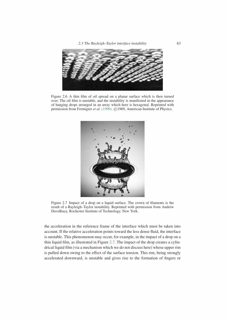
2.3 The Rayleigh–Taylor interface instability 63

Figure 2.6 A thin film of oil spread on a planar surface which is then turnedover. The oil film is unstable, and the instability is manifested in the appearanceof hanging drops arranged in an array which here is hexagonal. Reprinted withpermission from Fermigier et al. (1990). c©1969, American Institute of Physics.

Figure 2.7 Impact of a drop on a liquid surface. The crown of filaments is theresult of a Rayleigh–Taylor instability. Reprinted with permission from AndrewDavidhazy, Rochester Institute of Technology, New York.

the acceleration in the reference frame of the interface which must be taken intoaccount. If the relative acceleration points toward the less dense fluid, the interfaceis unstable. This phenomenon may occur, for example, in the impact of a drop on athin liquid film, as illustrated in Figure 2.7. The impact of the drop creates a cylin-drical liquid film (via a mechanism which we do not discuss here) whose upper rimis pulled down owing to the effect of the surface tension. This rim, being stronglyaccelerated downward, is unstable and gives rise to the formation of fingers or

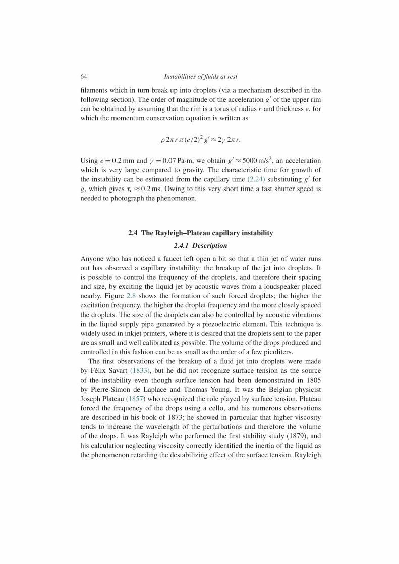
64 Instabilities of fluids at rest

filaments which in turn break up into droplets (via a mechanism described in thefollowing section). The order of magnitude of the acceleration g′ of the upper rimcan be obtained by assuming that the rim is a torus of radius r and thickness e, forwhich the momentum conservation equation is written as

ρ 2πr π(e/2)2 g′ ≈2γ 2πr.

Using e = 0.2 mm and γ = 0.07 Pa·m, we obtain g′ ≈ 5000 m/s2, an accelerationwhich is very large compared to gravity. The characteristic time for growth ofthe instability can be estimated from the capillary time (2.24) substituting g′ forg, which gives τc ≈ 0.2 ms. Owing to this very short time a fast shutter speed isneeded to photograph the phenomenon.

2.4 The Rayleigh–Plateau capillary instability

2.4.1 Description

Anyone who has noticed a faucet left open a bit so that a thin jet of water runsout has observed a capillary instability: the breakup of the jet into droplets. Itis possible to control the frequency of the droplets, and therefore their spacingand size, by exciting the liquid jet by acoustic waves from a loudspeaker placednearby. Figure 2.8 shows the formation of such forced droplets; the higher theexcitation frequency, the higher the droplet frequency and the more closely spacedthe droplets. The size of the droplets can also be controlled by acoustic vibrationsin the liquid supply pipe generated by a piezoelectric element. This technique iswidely used in inkjet printers, where it is desired that the droplets sent to the paperare as small and well calibrated as possible. The volume of the drops produced andcontrolled in this fashion can be as small as the order of a few picoliters.

The first observations of the breakup of a fluid jet into droplets were madeby Felix Savart (1833), but he did not recognize surface tension as the sourceof the instability even though surface tension had been demonstrated in 1805by Pierre-Simon de Laplace and Thomas Young. It was the Belgian physicistJoseph Plateau (1857) who recognized the role played by surface tension. Plateauforced the frequency of the drops using a cello, and his numerous observationsare described in his book of 1873; he showed in particular that higher viscositytends to increase the wavelength of the perturbations and therefore the volumeof the drops. It was Rayleigh who performed the first stability study (1879), andhis calculation neglecting viscosity correctly identified the inertia of the liquid asthe phenomenon retarding the destabilizing effect of the surface tension. Rayleigh

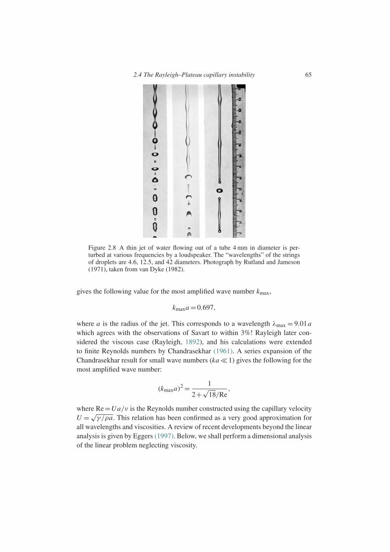
2.4 The Rayleigh–Plateau capillary instability 65

Figure 2.8 A thin jet of water flowing out of a tube 4 mm in diameter is per-turbed at various frequencies by a loudspeaker. The “wavelengths” of the stringsof droplets are 4.6, 12.5, and 42 diameters. Photograph by Rutland and Jameson(1971), taken from van Dyke (1982).

gives the following value for the most amplified wave number kmax,

kmaxa =0.697,

where a is the radius of the jet. This corresponds to a wavelength λmax = 9.01awhich agrees with the observations of Savart to within 3%! Rayleigh later con-sidered the viscous case (Rayleigh, 1892), and his calculations were extendedto finite Reynolds numbers by Chandrasekhar (1961). A series expansion of theChandrasekhar result for small wave numbers (ka 1) gives the following for themost amplified wave number:

(kmaxa)2 = 1

2+√18/Re

,

where Re=Ua/ν is the Reynolds number constructed using the capillary velocityU =√

γ /ρa. This relation has been confirmed as a very good approximation forall wavelengths and viscosities. A review of recent developments beyond the linearanalysis is given by Eggers (1997). Below, we shall perform a dimensional analysisof the linear problem neglecting viscosity.

66 Instabilities of fluids at rest

2.4.2 Dimensional analysis

As discussed above, surface tension stabilizes the planar interface between twolayers of superposed fluids subject to gravity. The reason for this is that any per-turbation of a planar interface increases its area A and therefore also the interfaceenergy γ A. In the present case of a cylindrical column the surface tension is, onthe contrary, destabilizing, and is responsible for the instability. Indeed, for a givenfixed volume of fluid, the interface area is smaller for an ensemble of sphericaldrops of radius r than for a cylinder of radius a; more precisely, the ratio of theareas of the drops formed from a cylinder of radius a is (Figure 2.9a)

area of drops

area of cylinder= 3

2

a

r.

Therefore, the ratio of the areas is smaller the larger the droplets: minimization ofthe interface area must lead to the largest possible drops. The instability thereforecorresponds to the transition to a state of smaller interface energy. However, theformation of large drops involves large displacements of fluid particles, displace-ments which are opposed by the fluid inertia (Figure 2.9). The droplet diameterthat results is therefore a compromise between a destabilizing factor, the surfacetension, and a stabilizing – or at least retarding – factor, the fluid inertia.

The droplet formation time can be estimated by dimensional analysis omittingviscous effects. We assume that the liquid column moves with constant velocity,and we consider the perturbed flow in the reference frame attached to the unper-turbed cylindrical column. The variables on which the problem depends are thenthe density ρ, the radius a of the column, and the surface tension γ . Thus the only

Figure 2.9 Capillary instability of a column of water: a perturbation of the inter-face is amplified owing to a capillary pressure gradient, thereby leading to dropletformation.

2.4 The Rayleigh–Plateau capillary instability 67

length and time scales are the radius a and the capillary time

τc =√ρa3/γ . (2.43)

We can then suppose that these scales give the orders of magnitude of the dropletdiameter and formation time. This droplet formation time grows with the dropletmass ρa3 and decreases with the surface tension, which seems reasonable. For a1 mm diameter water column, the time scale τc is a few milliseconds.

To make our discussion more precise, let us consider an axisymmetric pertur-bation of wavelength 2π/k and amplitude η of the cylindrical interface, as shownschematically in Figure 2.9b (this perturbation preserves the volume up to termsof order (η/a)2, which are negligible for small perturbations). If this wavelengthis small compared to the radius a, the perturbation “sees” a planar interface andso we have the case of a neutral capillary wave (zero growth rate). If, on the otherhand, the wavelength is large, the perturbation induces a difference of the radii ofcurvature: it is close to a −η at the necks and a +η at the bulges of the column.The difference of the curvatures, which can be written as

1

a −η− 1

a +η≈ 2η

a2

for small η/a, then leads to a pressure difference, according to the Laplace–Young law, of p+ − p− ≈ 2γ η/a2 and therefore to an average pressure gradient(k/π)(p+ − p−)≈ 2kγ η/πa2. This gradient induces an acceleration of the fluidtoward the bulges where the pressure is lower, which, from a one-dimensionalmomentum balance, is of order

du

dt∼ k(p+ − p−)

ρ∼ akη

τ 2c

,

where we have introduced the capillary time (2.43). Mass conservation givesanother equation relating velocity to displacement amplitude: the volume of fluidleaving a pinch during a time dt is of order ua2dt ; this decrease corresponds to avolume variation of order (a/k)dη, where dη is the variation of η during the timedt . We then deduce that ua2dt ∼ (a/k)dη, or

dη

dt∼ kau.

Differentiating the first equation with respect to time and taking into account thesecond, we obtain

d2u

dt2=σ 2u, σ ∼ ka

τc. (2.44)

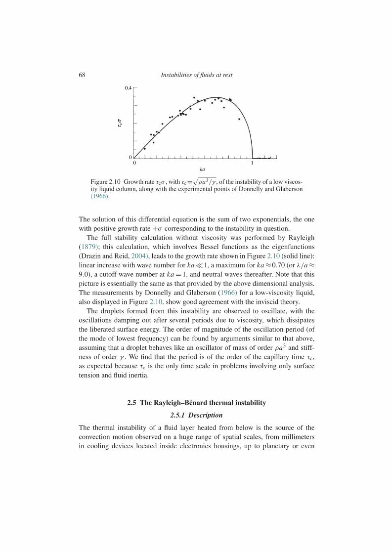
68 Instabilities of fluids at rest

0.4

τ cσ

00 1

ka

Figure 2.10 Growth rate τcσ , with τc =√ρa3/γ , of the instability of a low viscos-

ity liquid column, along with the experimental points of Donnelly and Glaberson(1966).

The solution of this differential equation is the sum of two exponentials, the onewith positive growth rate +σ corresponding to the instability in question.

The full stability calculation without viscosity was performed by Rayleigh(1879); this calculation, which involves Bessel functions as the eigenfunctions(Drazin and Reid, 2004), leads to the growth rate shown in Figure 2.10 (solid line):linear increase with wave number for ka 1, a maximum for ka ≈0.70 (or λ/a ≈9.0), a cutoff wave number at ka = 1, and neutral waves thereafter. Note that thispicture is essentially the same as that provided by the above dimensional analysis.The measurements by Donnelly and Glaberson (1966) for a low-viscosity liquid,also displayed in Figure 2.10, show good agreement with the inviscid theory.

The droplets formed from this instability are observed to oscillate, with theoscillations damping out after several periods due to viscosity, which dissipatesthe liberated surface energy. The order of magnitude of the oscillation period (ofthe mode of lowest frequency) can be found by arguments similar to that above,assuming that a droplet behaves like an oscillator of mass of order ρa3 and stiff-ness of order γ . We find that the period is of the order of the capillary time τc,as expected because τc is the only time scale in problems involving only surfacetension and fluid inertia.

2.5 The Rayleigh–Benard thermal instability

2.5.1 Description

The thermal instability of a fluid layer heated from below is the source of theconvection motion observed on a huge range of spatial scales, from millimetersin cooling devices located inside electronics housings, up to planetary or even

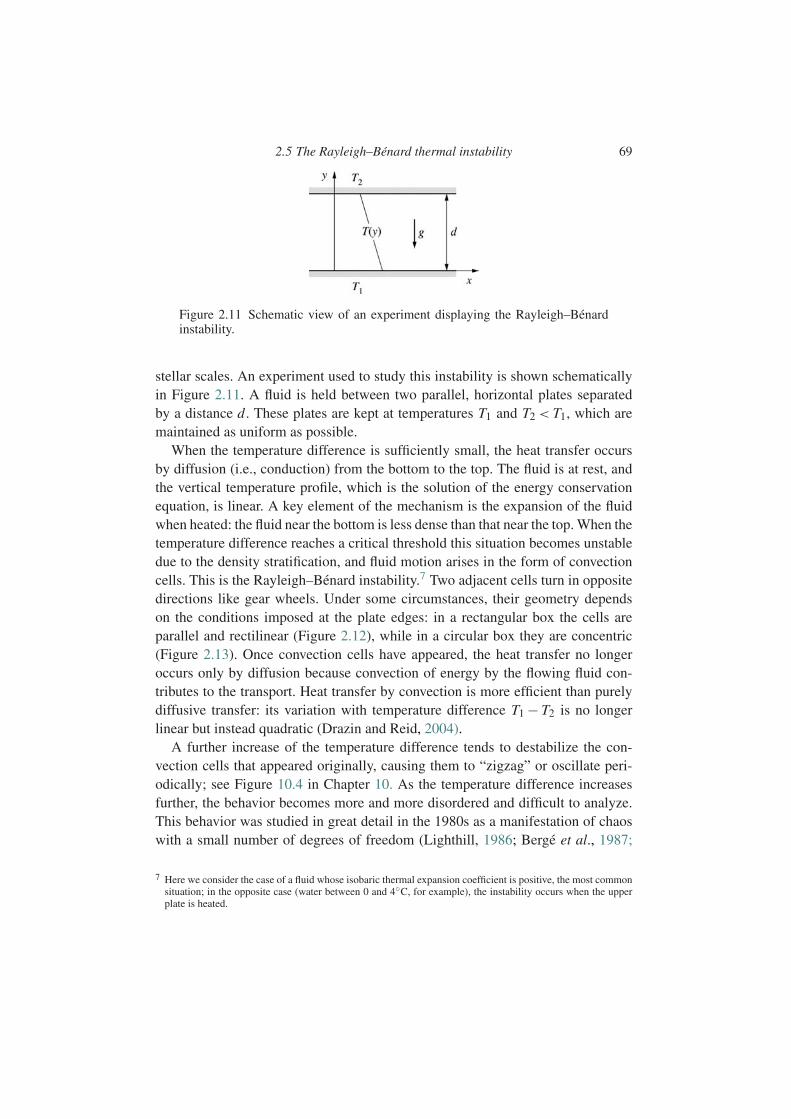
2.5 The Rayleigh–Benard thermal instability 69

Figure 2.11 Schematic view of an experiment displaying the Rayleigh–Benardinstability.

stellar scales. An experiment used to study this instability is shown schematicallyin Figure 2.11. A fluid is held between two parallel, horizontal plates separatedby a distance d. These plates are kept at temperatures T1 and T2 < T1, which aremaintained as uniform as possible.

When the temperature difference is sufficiently small, the heat transfer occursby diffusion (i.e., conduction) from the bottom to the top. The fluid is at rest, andthe vertical temperature profile, which is the solution of the energy conservationequation, is linear. A key element of the mechanism is the expansion of the fluidwhen heated: the fluid near the bottom is less dense than that near the top. When thetemperature difference reaches a critical threshold this situation becomes unstabledue to the density stratification, and fluid motion arises in the form of convectioncells. This is the Rayleigh–Benard instability.7 Two adjacent cells turn in oppositedirections like gear wheels. Under some circumstances, their geometry dependson the conditions imposed at the plate edges: in a rectangular box the cells areparallel and rectilinear (Figure 2.12), while in a circular box they are concentric(Figure 2.13). Once convection cells have appeared, the heat transfer no longeroccurs only by diffusion because convection of energy by the flowing fluid con-tributes to the transport. Heat transfer by convection is more efficient than purelydiffusive transfer: its variation with temperature difference T1 − T2 is no longerlinear but instead quadratic (Drazin and Reid, 2004).

A further increase of the temperature difference tends to destabilize the con-vection cells that appeared originally, causing them to “zigzag” or oscillate peri-odically; see Figure 10.4 in Chapter 10. As the temperature difference increasesfurther, the behavior becomes more and more disordered and difficult to analyze.This behavior was studied in great detail in the 1980s as a manifestation of chaoswith a small number of degrees of freedom (Lighthill, 1986; Berge et al., 1987;

7 Here we consider the case of a fluid whose isobaric thermal expansion coefficient is positive, the most commonsituation; in the opposite case (water between 0 and 4C, for example), the instability occurs when the upperplate is heated.

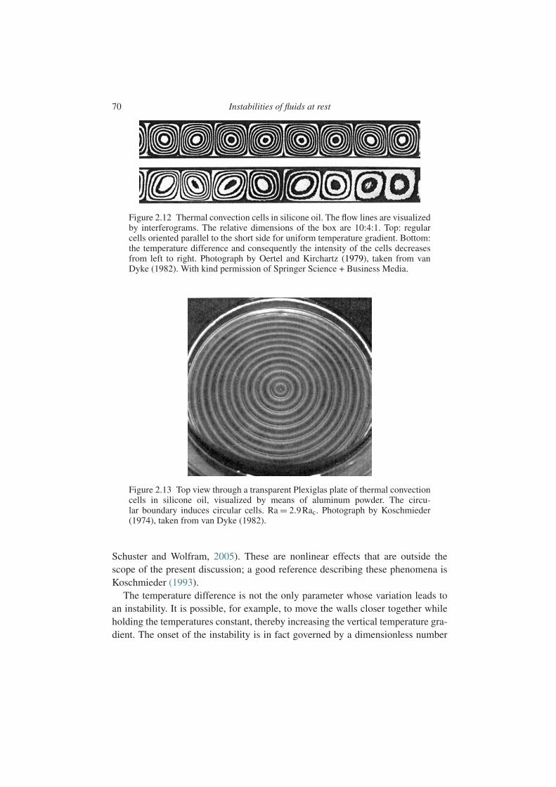
70 Instabilities of fluids at rest

Figure 2.12 Thermal convection cells in silicone oil. The flow lines are visualizedby interferograms. The relative dimensions of the box are 10:4:1. Top: regularcells oriented parallel to the short side for uniform temperature gradient. Bottom:the temperature difference and consequently the intensity of the cells decreasesfrom left to right. Photograph by Oertel and Kirchartz (1979), taken from vanDyke (1982). With kind permission of Springer Science + Business Media.

Figure 2.13 Top view through a transparent Plexiglas plate of thermal convectioncells in silicone oil, visualized by means of aluminum powder. The circu-lar boundary induces circular cells. Ra = 2.9Rac. Photograph by Koschmieder(1974), taken from van Dyke (1982).

Schuster and Wolfram, 2005). These are nonlinear effects that are outside thescope of the present discussion; a good reference describing these phenomena isKoschmieder (1993).

The temperature difference is not the only parameter whose variation leads toan instability. It is possible, for example, to move the walls closer together whileholding the temperatures constant, thereby increasing the vertical temperature gra-dient. The onset of the instability is in fact governed by a dimensionless number

2.5 The Rayleigh–Benard thermal instability 71

Figure 2.14 A fluid particle perturbed vertically in a temperature gradient.

called the Rayleigh number Ra which is the control parameter of the instabil-ity. This number, defined below, represents the net effect of two phenomena, onedestabilizing (the buoyancy force) and the other stabilizing (thermal diffusion).

2.5.2 The instability mechanism (Pr1)

Let us consider a small fluid particle of radius a d, temperature T , and densityρ, which, owing to fluctuations, is displaced upward a distance δy (Figure 2.14).The particle therefore finds itself surrounded by colder, denser fluid of temperatureT +δT and density ρ+δρ such that

δT = T2 −T1

dδy <0,

δρ =−αpρδT >0,

where αp is the isobaric thermal expansion coefficient of the fluid.8 The particle isthen subject to an upward-directed buoyancy force (the sum of its weight and theArchimedes force) equal to

FA = 4

3πa3δρg.

However, the resulting rising motion is counteracted by the viscous resistance.Let us consider the case of a fluid with high Prandtl number Pr = ν/κ , whereκ is the thermal diffusivity. Then the relaxation time of the particle motion, oforder a2/ν, is much shorter than the time during which the temperature differenceis maintained, which is of order a2/κ . The particle therefore reaches its equilib-rium speed v without the temperature having varied significantly. This equilibrium

8 The general equation of state is written as

δρ

ρ=−αpδT +κT δP,

where αp is the isobaric thermal expansion coefficient and κT is the isothermal compressibility, but herecompressibility effects are negligible.

72 Instabilities of fluids at rest

speed corresponds to equilibrium between the Archimedes force and the Stokesdrag force:

FS + FA =0, with FS ∝µav.

The equilibrium speed is therefore

v∝ αpga2 δT

ν. (2.46)

According to this equation, the speed v of the particle adapts very quickly to thetemperature difference δT , to which it is “enslaved.”

Two phenomena compete in the rising motion: thermal diffusion, which tendsto eliminate the temperature difference δT and therefore to stop the motion, andadvection at speed v toward the colder fluid which restores the temperature differ-ence and tends to amplify the motion. Marginal stability must correspond to thesetwo phenomena being in equilibrium, which is equivalent to the equality of theircharacteristic times. The time for thermal diffusion of the temperature difference isa2/κ , while that for restoration of this difference is δy/v, with δy/d =δT/(T1−T2)

and the velocity v given by (2.46). Thus, equal characteristic times corresponds to

a2

κ∝ ν d

αpga2(T1 −T2). (2.47)

This condition for marginal stability appears to depend on the particle radius a. Thedestabilizing force FA varies as a3 and the drag force FS as a and so the largestparticles are the first to be destabilized. For those with radius d/2 correspondingto the size of the observed convection cells, the marginal stability condition (2.47)can be written as Ra =Rac, where

Ra = αpg(T1 −T2)d3

νκ(2.48)

is known as the Rayleigh number, and Rac is a number corresponding to the criti-cal value of the Rayleigh number at the instability threshold. The actual numericalvalue of Rac cannot be obtained by dimensional analysis: the full calculation givesRac =1708 for rigid no-slip boundaries, a value independent of the Prandtl number.The important thing here is not the numerical value of the threshold, but the factthat we have found, by reasoning in terms of characteristic scales, a dimensionlessnumber controlling the onset of the instability. This key parameter has the phys-ical interpretation of the ratio of destabilizing to stabilizing forces. For Ra < Rac

thermal diffusion prevails over advection and any perturbation is dissipated, whilefor Ra>Rac the motion is amplified.

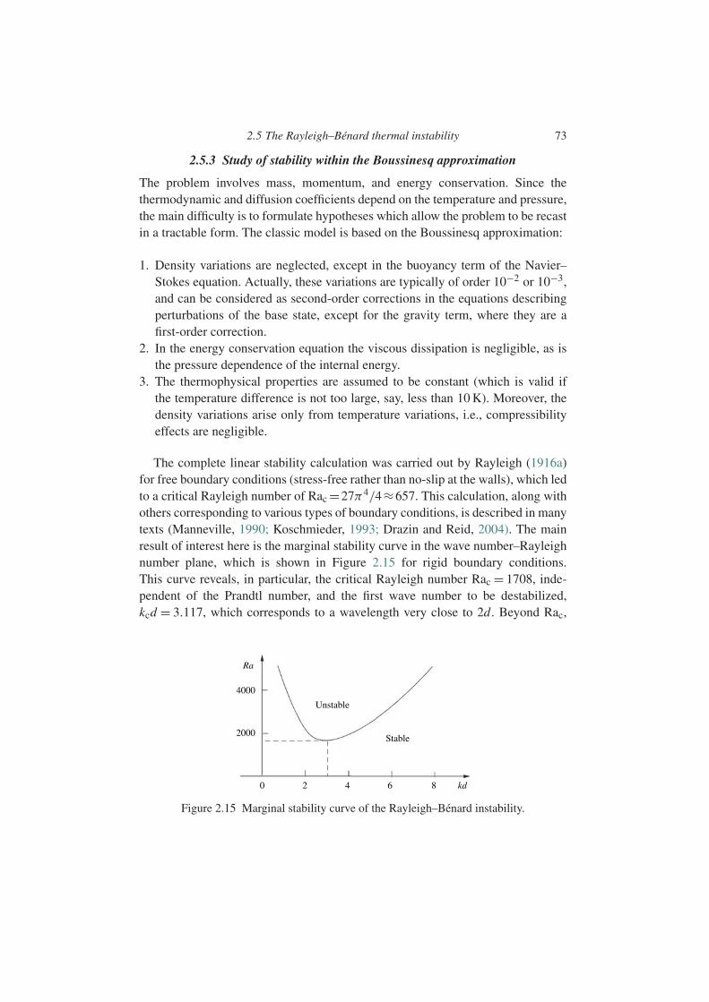
2.5 The Rayleigh–Benard thermal instability 73

2.5.3 Study of stability within the Boussinesq approximation

The problem involves mass, momentum, and energy conservation. Since thethermodynamic and diffusion coefficients depend on the temperature and pressure,the main difficulty is to formulate hypotheses which allow the problem to be recastin a tractable form. The classic model is based on the Boussinesq approximation:

1. Density variations are neglected, except in the buoyancy term of the Navier–Stokes equation. Actually, these variations are typically of order 10−2 or 10−3,and can be considered as second-order corrections in the equations describingperturbations of the base state, except for the gravity term, where they are afirst-order correction.

2. In the energy conservation equation the viscous dissipation is negligible, as isthe pressure dependence of the internal energy.

3. The thermophysical properties are assumed to be constant (which is valid ifthe temperature difference is not too large, say, less than 10 K). Moreover, thedensity variations arise only from temperature variations, i.e., compressibilityeffects are negligible.

The complete linear stability calculation was carried out by Rayleigh (1916a)for free boundary conditions (stress-free rather than no-slip at the walls), which ledto a critical Rayleigh number of Rac =27π4/4≈657. This calculation, along withothers corresponding to various types of boundary conditions, is described in manytexts (Manneville, 1990; Koschmieder, 1993; Drazin and Reid, 2004). The mainresult of interest here is the marginal stability curve in the wave number–Rayleighnumber plane, which is shown in Figure 2.15 for rigid boundary conditions.This curve reveals, in particular, the critical Rayleigh number Rac = 1708, inde-pendent of the Prandtl number, and the first wave number to be destabilized,kcd = 3.117, which corresponds to a wavelength very close to 2d. Beyond Rac,

2000

4000

Unstable

Stable

0 2 4 6 8 kd

Ra

Figure 2.15 Marginal stability curve of the Rayleigh–Benard instability.

74 Instabilities of fluids at rest

the width δk of the unstable band is centered at kc and grows as√

Ra−Rac.This result is in good agreement with experiments, which must be performedvery carefully to ensure, in particular, that the thermal conditions are uniform overthe plates.

Let us conclude by returning to the question of the instability mechanism. Wewrite down the two equations for vertical momentum conservation and energyconservation. Linearized about the base state, these two equations become

∂v

∂t=−∂y p

ρ+νv+αpg δT, (2.49a)

∂δT

∂t=κδT +v

T1 −T2

d. (2.49b)

In the first equation the first two terms on the right-hand side correspond to theretarding force induced by pressure and viscous drag,9 and the third correspondsto the buoyancy force. For Pr 1, where the velocity is quasi-statically slavedto the temperature disturbance, the equilibrium between these two forces corre-sponds to the dimensional equation (2.46) with ∼−1/a2. The second equation(2.49b) shows that the instability depends on the relative importance of the stabi-lizing thermal diffusion and the destabilizing advection. The equilibrium of thesetwo terms corresponds to the marginal stability condition given by the dimen-sional equation (2.47), again with ∼ −1/a2. Using the estimate (2.46) for thevelocity, from (2.49b) we find an estimate for the growth rate at large Prandtlnumber:

σ ∼ κ

d2

Ra−Rac

Rac. (2.50)

We note that this growth rate, the scale of which is the thermal diffusion time d2/κ ,is proportional to the distance from threshold Ra−Rac.

Rayleigh (1916a) thought that his calculation would explain the observationsmade by Benard (1900) of convection cells on thin layers of a liquid heated frombelow and open to air at the top. It was later realized that the instability whichRayleigh had found did not correspond to the situation studied by Benard, becausethe liquid layer was too thin and the dynamics involved surface tension. In thoseexperiments the instability is due not to the Archimedes force but to the surfacetension gradients generated by temperature nonuniformities of the free surface.This instability is discussed in the following section.

9 Here we note that the pressure gradient has the same scaling as the viscous force, as in all low Reynolds numberStokes flows. A well-known example is the force on a sphere in Stokes flow, where the two contributions areexactly equal to 3πµav.

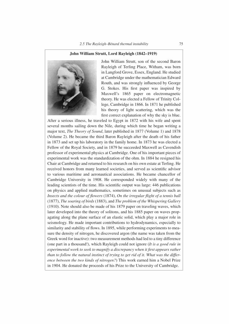
2.5 The Rayleigh–Benard thermal instability 75

John William Strutt, Lord Rayleigh (1842–1919)

John William Strutt, son of the second BaronRayleigh of Terling Place, Witham, was bornin Langford Grove, Essex, England. He studiedat Cambridge under the mathematician EdwardRouth, and was strongly influenced by GeorgeG. Stokes. His first paper was inspired byMaxwell’s 1865 paper on electromagnetictheory. He was elected a Fellow of Trinity Col-lege, Cambridge in 1866. In 1871 he publishedhis theory of light scattering, which was thefirst correct explanation of why the sky is blue.

After a serious illness, he traveled to Egypt in 1872 with his wife and spentseveral months sailing down the Nile, during which time he began writing amajor text, The Theory of Sound, later published in 1877 (Volume 1) and 1878(Volume 2). He became the third Baron Rayleigh after the death of his fatherin 1873 and set up his laboratory in the family home. In 1873 he was elected aFellow of the Royal Society, and in 1879 he succeeded Maxwell as Cavendishprofessor of experimental physics at Cambridge. One of his important pieces ofexperimental work was the standardization of the ohm. In 1884 he resigned hisChair at Cambridge and returned to his research on his own estate at Terling. Hereceived honors from many learned societies, and served as scientific advisorto various maritime and aeronautical associations. He became chancellor ofCambridge University in 1908. He corresponded widely with many of theleading scientists of the time. His scientific output was large: 446 publicationson physics and applied mathematics, sometimes on unusual subjects such asInsects and the colour of flowers (1874), On the irregular flight of a tennis ball(1877), The soaring of birds (1883), and The problem of the Whispering Gallery(1910). Note should also be made of his 1879 paper on traveling waves, whichlater developed into the theory of solitons, and his 1885 paper on waves prop-agating along the plane surface of an elastic solid, which play a major role inseismology. He made important contributions to hydrodynamics, especially tosimilarity and stability of flows. In 1895, while performing experiments to mea-sure the density of nitrogen, he discovered argon (the name was taken from theGreek word for inactive): two measurement methods had led to a tiny difference(one part in a thousand!), which Rayleigh could not ignore (It is a good rule inexperimental work to seek to magnify a discrepancy when it first appears ratherthan to follow the natural instinct of trying to get rid of it. What was the differ-ence between the two kinds of nitrogen?) This work earned him a Nobel Prizein 1904. He donated the proceeds of his Prize to the University of Cambridge.

76 Instabilities of fluids at rest

2.6 The Benard–Marangoni thermocapillary instability

2.6.1 Description

When a thin layer of liquid open to the air is heated by the plate on which it rests,an instability arises in the form of convection cells, which are generally hexag-onal as shown in Figures 2.16 and 2.17. It should be observed in Figure 2.16how the hexagonal cells adapt themselves to a circular boundary, and also how aflower-like imperfection is formed, at the right center, owing to a tiny perturbationon the lower copper plate. This convection phenomenon, discovered and studiedby Benard (1900), resembles the Rayleigh–Benard instability described above inthat it occurs in a heated liquid, but its physical origin is different: it originates notwith the buoyant force, but from gradients of the surface tension due to temperaturenonuniformities. Thus the presence of a free surface is essential. This thermocap-illary instability is now associated with the name of the Italian physicist CarloMarangoni (1871), who noticed that a surface tension gradient induced by a tem-perature gradient or a concentration gradient in an aqueous solution can generatefluid motion, a phenomenon now known as the Marangoni effect (Probstein, 2003).The correct interpretation of the Benard experiments is due to Pearson (1958).

Since the mechanism of this thermocapillary instability is associated withthe variation of the surface tension with temperature, we need to describe thisvariation. For a liquid in equilibrium with its vapor or with air, the followingapproximate equation of state is well satisfied over a large temperature range(Rocard, 1967):

γ =γ0

(1− 1.03 T

Tc

), (2.51)

Figure 2.16 Thermocapillary convection cells in a thin layer of silicone oil ofviscosity 0.5 cm2/s. Photograph by Koschmieder (1974), taken from van Dyke(1982).

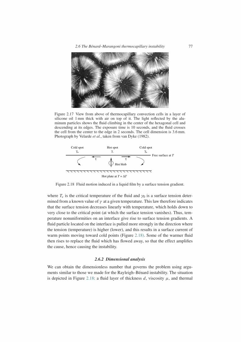
2.6 The Benard–Marangoni thermocapillary instability 77

Figure 2.17 View from above of thermocapillary convection cells in a layer ofsilicone oil 1 mm thick with air on top of it. The light reflected by the alu-minum particles shows the fluid climbing in the center of the hexagonal cell anddescending at its edges. The exposure time is 10 seconds, and the fluid crossesthe cell from the center to the edge in 2 seconds. The cell dimension is 3.6 mm.Photograph by Velarde et al., taken from van Dyke (1982).

Cold spotγ+

Cold spotγ+

Free surface at T

Hot spotγ–

Hot blob

τ τ

Hot plate at T + ∆T

Figure 2.18 Fluid motion induced in a liquid film by a surface tension gradient.

where Tc is the critical temperature of the fluid and γ0 is a surface tension deter-mined from a known value of γ at a given temperature. This law therefore indicatesthat the surface tension decreases linearly with temperature, which holds down tovery close to the critical point (at which the surface tension vanishes). Thus, tem-perature nonuniformities on an interface give rise to surface tension gradients. Afluid particle located on the interface is pulled more strongly in the direction wherethe tension (temperature) is higher (lower), and this results in a surface current ofwarm points moving toward cold points (Figure 2.18). Some of the warmer fluidthen rises to replace the fluid which has flowed away, so that the effect amplifiesthe cause, hence causing the instability.

2.6.2 Dimensional analysis

We can obtain the dimensionless number that governs the problem using argu-ments similar to those we made for the Rayleigh–Benard instability. The situationis depicted in Figure 2.18: a fluid layer of thickness d, viscosity µ, and thermal

78 Instabilities of fluids at rest

diffusivity κ is subject to a temperature difference T >0 between the lower plateand the free surface. Now consider a fluctuation in the form of a fluid upwellingthat brings a patch of hot fluid to the surface. This will raise the temperature thereby an amount on the order of T relative to the undisturbed surface temperature.The warmer fluid will have a lower interfacial tension relative to the colder pointon the surface (where the fluid must down-well in order to conserve mass). Thescaling estimates that follow can be developed with the wavelength of the convec-tion, λ, different from the depth, d, but for simplicity we take these length scalesto be the same order of magnitude.

The temperature gradient results in a horizontal Marangoni shearing stress,

τ ∼ dγ

dx∼γ ′ T

d.

The tangential force (per unit length in the direction perpendicular to the plane)due to the applied Marangoni stress is therefore

Fγ ∼γ ′T .

The question is now whether the viscous drag on the blob and diffusion of tempera-ture are both small enough to allow a sustained circulation driven by the Marangonistress produced by the initial upwelling. The viscous drag per unit length is

Fµ ∼µ |∇2u|d2 ∼µu.

If the convection is to be self-sustaining the convection of energy must competewith thermal diffusion, i.e.

u ·∇T ∼κ∇2T,

from which we determine the velocity scale as

u ∼κ/d.

Eliminating the velocity, the ratio of the driving force to the retarding forcebecomes

Fγ

Fµ

∼ γ ′T d

κµ=Ma. (2.52)

This dimensionless number is known as the Marangoni number, and governs avariety of thermocapillary flows. The review of Schatz and Neitzel (2001) canbe consulted for a more complete analysis of this and other thermocapillaryinstabilities.

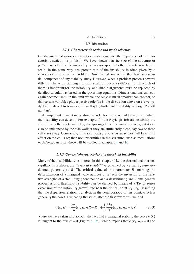
2.7 Discussion 79

2.7 Discussion

2.7.1 Characteristic scales and mode selection

Our discussion of various instabilities has demonstrated the importance of the char-acteristic scales in a problem. We have shown that the size of the structure orpattern selected by the instability often corresponds to the characteristic lengthscale. In the same way, the growth rate of the instability is often given by acharacteristic time in the problem. Dimensional analysis is therefore an essen-tial component of any stability study. However, when a problem presents severaldifferent characteristic length or time scales, it becomes difficult to tell which ofthem is important for the instability, and simple arguments must be replaced bydetailed calculations based on the governing equations. Dimensional analysis canagain become useful in the limit where one scale is much smaller than another, sothat certain variables play a passive role (as in the discussion above on the veloc-ity being slaved to temperature in Rayleigh–Benard instability at large Prandtlnumber).

An important element in the structure selection is the size of the region in whichthe instability can develop. For example, for the Rayleigh–Benard instability thesize of the cells is determined by the spacing of the horizontal surfaces, but it canalso be influenced by the side walls if they are sufficiently close, say two or threecell sizes away. Conversely, if the side walls are very far away they will have littleeffect on the cell size; then nonuniformities in the structure, such as modulationsor defects, can arise; these will be studied in Chapters 9 and 10.

2.7.2 General characteristics of a threshold instability

Many of the instabilities encountered in this chapter, like the thermal and thermo-capillary instabilities, are threshold instabilities governed by a control parameterdenoted generally as R. The critical value of this parameter Rc marking thedestabilization of a marginal wave number kc reflects the inversion of the rela-tive strengths of a stabilizing phenomenon and a destabilizing one. Some generalproperties of a threshold instability can be derived by means of a Taylor seriesexpansion of the instability growth rate near the critical point (kc, Rc) (assumingthat the dispersion relation is analytic in the neighborhood of this point, which isgenerally the case). Truncating the series after the first few terms, we find

σ(k, R)= ∂σ

∂R(kc, Rc)(R − Rc)+ 1

2

∂2σ

∂k2(kc, Rc)(k −kc)

2, (2.53)

where we have taken into account the fact that at marginal stability the curve σ(k)is tangent to the axis σ = 0 (Figure 2.19a), which implies that σ(kc, Rc)= 0 and

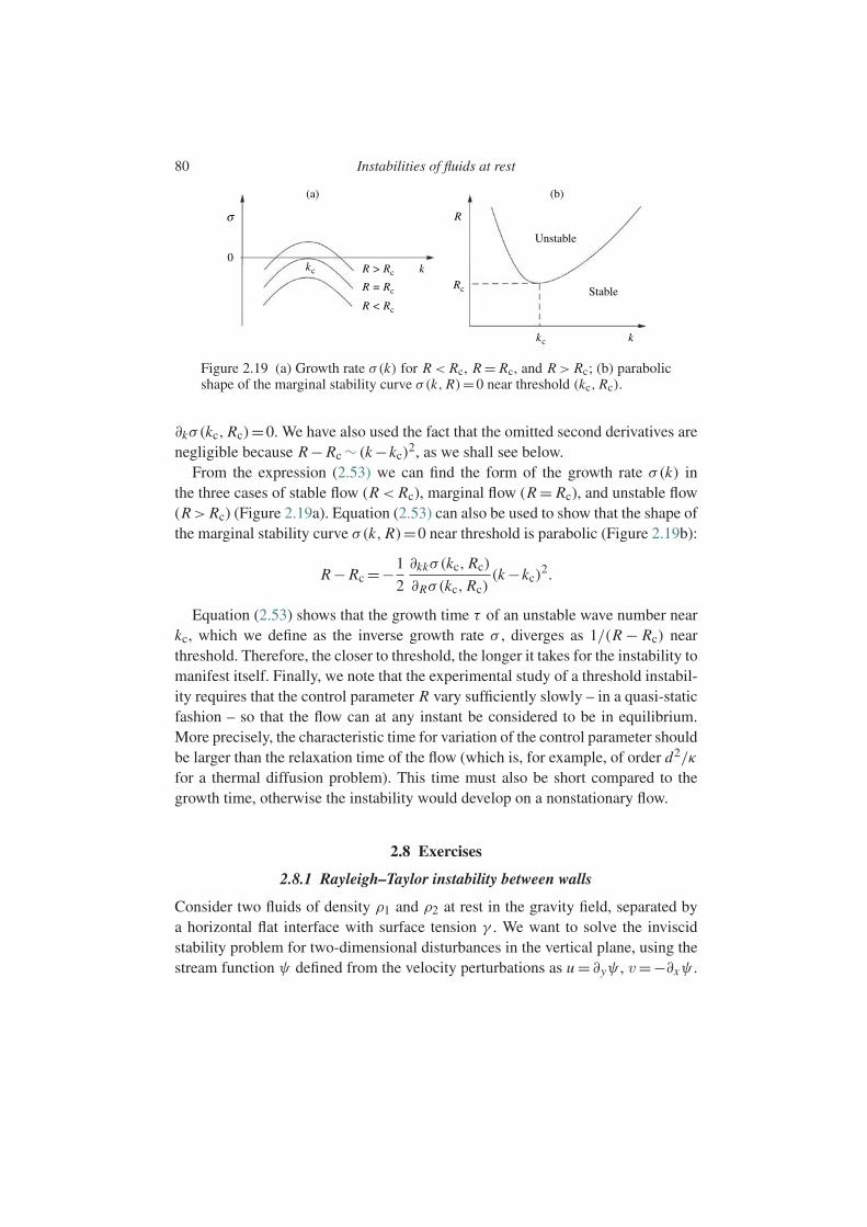
80 Instabilities of fluids at rest

(a)

0

σ

(b)

Unstable

Stable

R

Rc

R > Rc

R < Rc

R = Rc

k

kc

kc

k

Figure 2.19 (a) Growth rate σ(k) for R < Rc, R = Rc, and R > Rc; (b) parabolicshape of the marginal stability curve σ(k, R)=0 near threshold (kc, Rc).

∂kσ(kc, Rc)=0. We have also used the fact that the omitted second derivatives arenegligible because R − Rc ∼ (k −kc)

2, as we shall see below.From the expression (2.53) we can find the form of the growth rate σ(k) in

the three cases of stable flow (R < Rc), marginal flow (R = Rc), and unstable flow(R> Rc) (Figure 2.19a). Equation (2.53) can also be used to show that the shape ofthe marginal stability curve σ(k, R)=0 near threshold is parabolic (Figure 2.19b):

R − Rc =−1

2

∂kkσ(kc, Rc)

∂Rσ(kc, Rc)(k −kc)

2.

Equation (2.53) shows that the growth time τ of an unstable wave number nearkc, which we define as the inverse growth rate σ , diverges as 1/(R − Rc) nearthreshold. Therefore, the closer to threshold, the longer it takes for the instability tomanifest itself. Finally, we note that the experimental study of a threshold instabil-ity requires that the control parameter R vary sufficiently slowly – in a quasi-staticfashion – so that the flow can at any instant be considered to be in equilibrium.More precisely, the characteristic time for variation of the control parameter shouldbe larger than the relaxation time of the flow (which is, for example, of order d2/κ

for a thermal diffusion problem). This time must also be short compared to thegrowth time, otherwise the instability would develop on a nonstationary flow.

2.8 Exercises

2.8.1 Rayleigh–Taylor instability between walls

Consider two fluids of density ρ1 and ρ2 at rest in the gravity field, separated bya horizontal flat interface with surface tension γ . We want to solve the inviscidstability problem for two-dimensional disturbances in the vertical plane, using thestream function ψ defined from the velocity perturbations as u = ∂yψ , v=−∂xψ .

2.8 Exercises 81

1. Show that in the case of unbounded layers (infinite depths), the dispersionrelation is given by (2.40).

2. For bounded layers of thicknesses h1 and h2, show that the dispersion relation is

c2(ρ1 cothkh1 +ρ2 cothkh2)− [(ρ1 −ρ2)g/k +γ k]=0.

3. Compare the cases of finite and infinite depths: is the band of unstable wavenumbers different? How does the growth rate vary for k small? The solutioncan be found in Milne-Thompson (1968).

2.8.2 Instability of a suspended thin film

Consider a thin liquid film of thickness h, viscosity µ, and density ρ, applied tothe underside of a horizontal wall in the gravity field g=−gey . We shall study thestability of this film to two-dimensional perturbations in the vertical plane (x, y).The free surface of the unperturbed film is defined by y = 0 (the surface to whichthe film is applied is therefore at y =h), and so the pressure is P = P0−ρgy, whereP0 is the air pressure under the film.

We study perturbations of wavelength large compared to the film thickness(kh 1) (∂x u + ∂yv = 0 implies that v ∼ (kh)u u, so that the flow is quasi-parallel), and we also assume that the flow is quasi-static, that is, it adapts veryrapidly to the boundary conditions: time enters only through the condition at thedeformed free surface η(x, t)= ηei(kx−ωt)+c.c.

1. Show that the linearized equations for perturbations of the base state are

0=−∂x p+µ∂yyu, 0=−∂y p.

2. We recall that the components of the stress tensor of a Newtonian fluid aregiven by σi j =−Pδi j +µ(∂x j Ui +∂xi U j ). Assuming that the air under the filmimposes only its pressure P0 (the free surface condition), show that, after lin-earization about y = 0, the boundary conditions tangential and normal to thefree surface y =η(x, t) can be written as

∂yu =0, p−ρgη=γ ∂xxη.

3. Using the boundary conditions at y =h and at the free surface, find the speed uas a function of the pressure gradient ∂x p.

4. Determine the speed v as a function of the pressure gradient ∂x p.

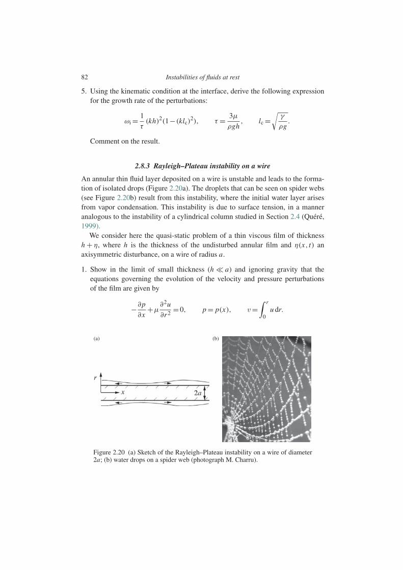
82 Instabilities of fluids at rest

5. Using the kinematic condition at the interface, derive the following expressionfor the growth rate of the perturbations:

ωi = 1

τ(kh)2(1−(klc)

2), τ = 3µ

ρgh, lc =

√γ

ρg.

Comment on the result.

2.8.3 Rayleigh–Plateau instability on a wire

An annular thin fluid layer deposited on a wire is unstable and leads to the forma-tion of isolated drops (Figure 2.20a). The droplets that can be seen on spider webs(see Figure 2.20b) result from this instability, where the initial water layer arisesfrom vapor condensation. This instability is due to surface tension, in a manneranalogous to the instability of a cylindrical column studied in Section 2.4 (Quere,1999).

We consider here the quasi-static problem of a thin viscous film of thicknessh + η, where h is the thickness of the undisturbed annular film and η(x, t) anaxisymmetric disturbance, on a wire of radius a.

1. Show in the limit of small thickness (h a) and ignoring gravity that theequations governing the evolution of the velocity and pressure perturbationsof the film are given by

−∂p

∂x+µ

∂2u

∂r2=0, p = p(x), v=

∫ r

0u dr.

(b)(a)

Figure 2.20 (a) Sketch of the Rayleigh–Plateau instability on a wire of diameter2a; (b) water drops on a spider web (photograph M. Charru).

2.8 Exercises 83

Also show that the relevant boundary conditions are no-slip, u = v= 0, on thewire at r = a, and the following linearized conditions at the free surface atr =a +h:

µ∂u

∂r=0, p =γ

(− η

a2− ∂2η

∂x2

).

2. Introducing time-independent normal modes except for η (which is the samequasi-static approximation as in the previous exercise), show that the growthrate of the disturbances is

σ = 1

τ

(h

a

)3

(ka)2 (1−(ka)2), τ = 3µa

γ.

3. Discuss the stability, and in particular determine the most amplified and thecutoff wave numbers.

2.8.4 Stability of a planar front between two fluids in a porous medium

When a viscous fluid 2 is pushed by another less viscous fluid 1 in a porousmedium or in a Hele–Shaw cell (Figure 2.21), the initially rectilinear front is unsta-ble to the growth of fingers, as shown in Figure 2.22. This phenomenon is known as“viscous fingering” (Homsy, 1987). We want to determine the linear stability con-dition of the horizontal front between the two fluids (Saffman and Taylor, 1958).The motion of each fluid is governed by the Darcy equation

U j =− K

µ jgrad(Pj +ρ j gy), j =1,2, (2.54)

where ρ j and µ j are the density and viscosity of fluid j , and K is the permeability,assumed uniform, of the porous medium. The thickness of the front is assumed tobe negligible compared to the other characteristic lengths of the problem. Viscous

Fluid 2 Fluid 2yy

x x

Fluid 1 Fluid 1

Perturbed frontFlat front

gn

Figure 2.21 Front between two viscous fluids in a porous medium or a Hele–Shaw cell.

84 Instabilities of fluids at rest

Figure 2.22 Two different stages of the growth of the Saffman–Taylor instabilityin a vertical Hele–Shaw cell, at the interface between glycerin pushed down byair above. The cell cross-section is 0.9 mm × 120 mm and the descending speedof the front is V ≈1 mm/s (Saffman and Taylor, 1958).

stresses are negligible compared to pressure, and we also neglect surface tension,leaving only a pressure continuity condition at the front between the fluids.

1. Using the Darcy equation, show that there exists a velocity potential j andfind the equation it satisfies.

2. Show that the problem has the basic solution

j = V z, P j =−(µ j V

K+ρ j g

)z + P0(t), (2.55)

where V is the uniform velocity of ascension of the fluids, z = y − V t is thedistance to the unperturbed front, and P0(t) is a reference pressure on the front.

3. Determine the linearized equations for small perturbations of the potential,φ j (x, z, t), pressure, p j (x, z, t), and front position, h(x, t), i.e., the mass con-servation and Darcy equations and the boundary conditions (i) at z = ±∞and (ii) on the front (continuity of the normal velocity and the pressure, andimpermeability of the front).

4. Introduce perturbations proportional to exp(ikx +σ t) with k real. Justify thechosen form, state the meaning of k and σ , and write down the system ofequations satisfied by the amplitudes of the perturbations. Solve this system

2.8 Exercises 85

and derive the dispersion relation

σ = kK

µ1 +µ2

(µ2 −µ1

KV +(ρ2 −ρ1)g

). (2.56)

5. Sketch the possible shapes of σ(k) for ρ1 =ρ2, and then for ρ1 =ρ2. Commenton this. Is the divergence of σ(k) at large k physical? Beyond what order ofmagnitude of wave number is the model no longer valid?

6. We want to extract oil (ρ2 = 900 kg/m3, µ2 = 0.1 Pa·s) from a porous mediumof permeability K = 10 Darcys (1 Darcy = 10−12 m2) by injecting water to thebottom of a well (ρ1 = 1000 kg/m3, µ1 =10−3 Pa·s). Beyond what speed is theflow unstable? For a speed of 1 cm/s, how long does it take for the amplitude ofa perturbation of wave number k =1 cm−1 to be multiplied by 10?

We finally note that a similar analysis is possible for the “printer’s instabil-ity.” Consider counter-rotating horizontal cylinders immersed in a bath of viscousliquid. The rotation of the cylinders entrains thin films of fluid which cover thecylinders. The film with uniform thickness appears to be unstable, showing peri-odic variations of its thickness along the cylinder axes (Rabaud et al., 1990;Couder, 2000). This instability can be interpreted as a Saffman–Taylor instabilityin a wedge (Ruschak, 1985).

2.8.5 The Darrieus–Landau instability of a flame front

The front of the flame separating premixed, gaseous reactants, from burnt gas canbe unstable. This instability has been studied theoretically by Darrieus (1938) andlater by Landau (1944), and has been displayed in a well-controlled experimentby Clanet and Searby (1998). On the left of Figure 2.23 is the experimental setup.An air–propane mixture is injected into the bottom of a vertical tube, and the burntgas escapes from the top. The planar flame front is excited by an acoustic wavegenerated by a loudspeaker, and its position is recorded by a fast camera. Theamplification with time of the front perturbation selected by the excitation is seenin the photographs shown on the right.

The situation is shown schematically in Figure 2.24. The equations governingthe problem admit a stationary solution in a reference frame attached to the planarfront, with uniform velocities U 1 at the upstream end and U 2 at the downstreamend. We make the following assumptions about the perturbed flow (Landau andLifshitz, 1987, §128; Joulin and Vidal, 1998):

• the flow is incompressible on each side of the front, and viscous effects can beneglected;

• the density of each gas remains uniform, with ρ1 >ρ2;

86 Instabilities of fluids at rest

Figure 2.23 Experimental demonstration of the Darrieus–Landau instability.Figure reprinted with permission from Clanet and Searby (1998). c©1998 by theAmerican Physical Society. Left: schematic view of the setup. Right: growth withtime of the eigenmode selected by the excitation.

y y

n

x

Unburnt gas Burnt gas

Flat front Perturbed front

x

Figure 2.24 Flow through a planar flame front and a perturbed flame front.

• the relative local speed UL of the flame front relative to the incoming reactants(a few meters per second) is constant;

• the thickness of the flame front (less than one millimeter) is very small comparedto the wavelength of the perturbations.

The equations governing the problem are therefore the Euler equations:

divU j =0, (2.57a)

ρ j (∂t U j +(U j ·grad)U j )=−grad Pj , j =1,2. (2.57b)

2.8 Exercises 87

The boundary conditions are decay of the perturbations at infinity both upstreamand downstream, along with the following jump conditions at the flame front x =η(y, t):

ρ1(U1 −w) ·n=ρ2(U2 −w) ·n , (2.58a)

P1 +ρ1 ((U1 −w) ·n)2 = P2 +ρ2 ((U2 −w) ·n)2 , (2.58b)

U1 ×n=U2 ×n , (2.58c)

(U1 −w) ·n=UL . (2.58d)

Defining the position of the front as H(x, y, t)= x −η(y, t)=0, the normal n andthe normal velocity w ·n at the front are obtained from (2.30) and (2.31).

1. State the physical meaning of the four jump conditions listed above. Sketcha streamline which crosses the front obliquely. By analogy with geometricaloptics, what should this phenomenon be called?

2. Show that the base flow given by

U 1 =UL ,

U 2 = ρ1

ρ2UL ,

P2 = P1 +ρ1U21 −ρ2U

22 ,

satisfies the conservation equations and jump conditions.3. Write down the linearized equations for small perturbations of the base flow.4. Introduce perturbations in the form of normal modes proportional to exp(iky +

σ t) with k real. Justify the choice of this form, give the meaning of k and σ , andwrite down the system of equations satisfied by the amplitudes of the normalmodes.

5. Find the general solution for the amplitudes of the normal modes, taking intoconsideration their decay at infinity upstream and downstream (in anticipationchoose σ >0, a hypothesis to be verified at the end of the calculation).

6. Write the system of four algebraic equations corresponding to the jumpconditions at the flame front, and show that the dispersion relation can bewritten as

(1+r)σ 2 +2rkULσ +r(1−r)k2U 2L =0 (2.60)

where r =ρ1/ρ2.7. Discuss the type of the eigenvalues and sketch the shape of σ(k). Is the diver-

gence of σ(k) at large k physical? What is the length scale, not taken intoaccount in the above model, below which the model is no longer valid?

3

Stability of open flows: basic ideas

3.1 Introduction

In this chapter we begin our study of the stability of flows. We start by makingour discussion of linear stability introduced in Chapter 2 more precise (Section3.1). The approach for deciding whether a flow is stable or unstable on the basis oftemporal normal modes is justified by studying the spatio-temporal evolution of anarbitrary perturbation (Section 3.2). In the case of open flows, where a perturba-tion never passes the same point more than once (in contrast to closed flow such asCouette flow between two cylinders), we distinguish two types of instability: con-vective and absolute (Section 3.3). The ideas introduced in a rather abstract way inthis chapter will be illustrated more concretely in the following chapters.

3.1.1 Linear dynamics of a wave packet

We have seen that in many cases, normal mode analysis admits the possibility ofstable or unstable propagating waves. Here we shall derive some classical resultson the propagation of a packet of dispersive waves for the special case of a Gaus-sian packet. A more general discussion can be found in, for example, Lighthill(1978, §3.7). We consider a wave represented by the integral of its spatial Fouriercomponents

u(x, t)= 1

2

∫ +∞

−∞u(k)ei(kx−ω(k)t)dk, (3.1)

where the wave number k and frequency ω(k) are real and u(k) is the spectrum ofthe wave packet.1 Assuming that the waves propagate at positive speed c =ω/k,we choose the corresponding branch of the dispersion relation, namely, the one for

1 This spectrum does not correspond exactly to the Fourier transform of u(x) owing to the factor of 1/π whichfor convenience we have omitted from (3.1).

88

3.1 Introduction 89

which ω(k) has the same sign as k. Then, using the relation u(−k)= u∗(k), theabove integral can be rewritten as

u(x, t)= 1

2

∫ +∞

0u(k)ei(kx−ω(k)t)dk +c.c. (3.2)

For x large and x/t fixed, this integral can be evaluated using the method of sta-tionary phase.2 It can also be evaluated directly in the case of a Gaussian spectrumof width σ−1 centered on a wave number k0 (Figure 3.1a), i.e.

u(k)= u0 e−σ 2(k−k0)2, k >0. (3.3)

A Gaussian spectrum is typical of many experimental situations and leads to sim-ple calculations of the wave evolution: in particular, the Fourier transform of aGaussian is also a Gaussian. The wave (3.2) can also be written as a travelingwave of wave number k0 and frequency ω0 =ω(k0):

u(x, t)= 1

2A(x, t)ei(k0x−ω0t)+c.c., (3.4)

where A(x, t) is the envelope of the wave packet, defined as

A(x, t)=∫ ∞

0u(k)ei(k−k0)x−i(ω−ω0)t dk. (3.5)

This envelope depends on space and time, and so it differs from the amplitude ofa Fourier mode, which can depend on time but is spatially uniform.

The wave envelope at the initial time

Setting v=σ(k −k0 − ix/2σ 2), the argument of the exponential inside the integral(3.5) can be written at the initial time t =0 as

−σ 2(k −k0)2 + i(k −k0)x =−v2 − x2

4σ 2. (3.6)

2 We consider the integral I (x)=∫ k2k1

f (k)eixψ(k) dk. When there exists a number k0 inside the integration range

such that ψ(p)(k0) =0 but ψ ′(k0)= ...=ψ(p−1)(k0)=0 with f (k0) =0, then for x large (Bender and Orszag,1978, §6.5)

I (x)∼2 f (k0)exp(ixψ(k0)± iπ/2p)

(p

x |ψ(p)(k0)|)1/p (1/p)

p,

where we use the factor eiπ/2p if ψ(p)(k0) > 0, or the factor e−iπ/2p if ψ(p)(k0) < 0. The usual casecorresponds to p =2, for which (1/2)=√

π .

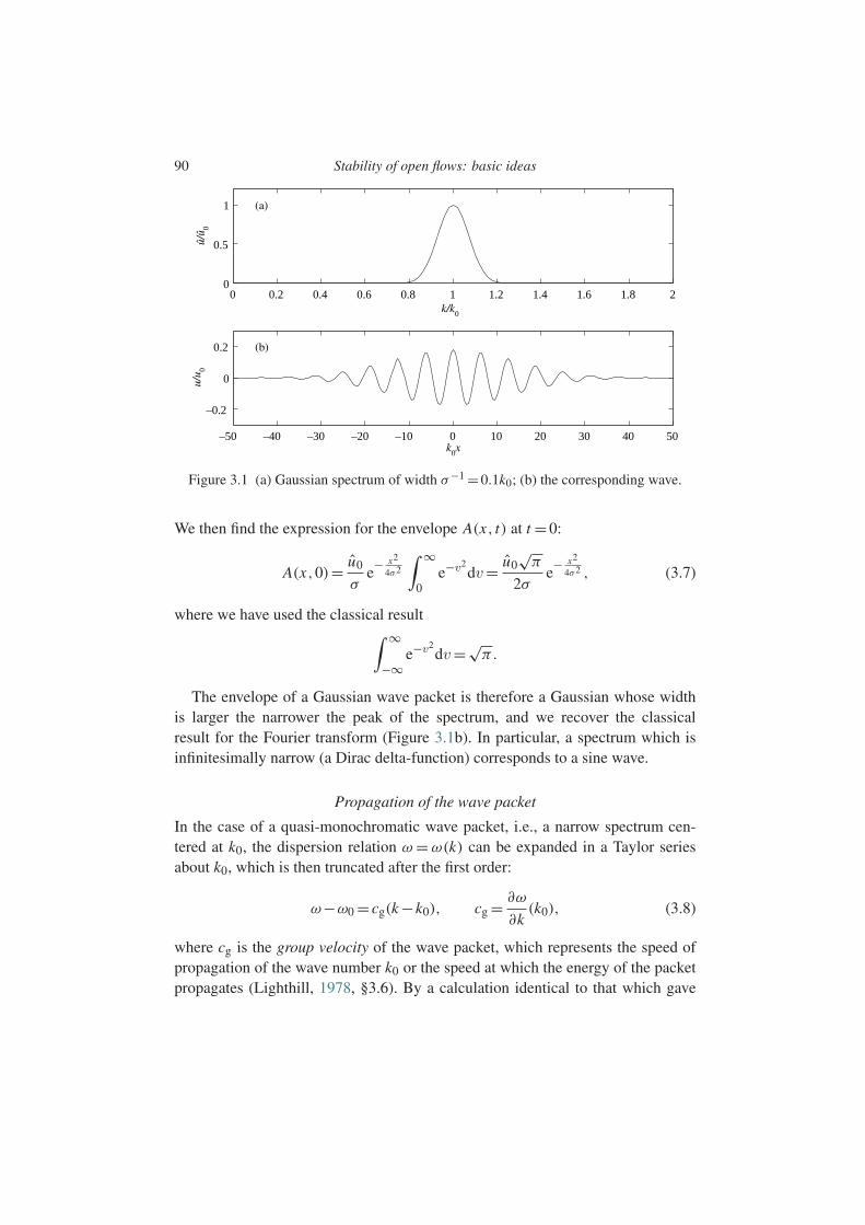
90 Stability of open flows: basic ideas

0 0.2 0.4 0.6 0.8 1 1.2 1.4 1.6 1.8 20

0.5

1

k/k0

k0x

û 0/û

(a)

–50 –40 –30 –20 –10 0 10 20 30 40 50

–0.2

0

0.2

u 0/u

(b)

Figure 3.1 (a) Gaussian spectrum of width σ−1 =0.1k0; (b) the corresponding wave.

We then find the expression for the envelope A(x, t) at t =0:

A(x,0)= u0

σe− x2

4σ2

∫ ∞

0e−v2

dv= u0√π

2σe− x2

4σ2 , (3.7)

where we have used the classical result∫ ∞

−∞e−v2

dv=√π.

The envelope of a Gaussian wave packet is therefore a Gaussian whose widthis larger the narrower the peak of the spectrum, and we recover the classicalresult for the Fourier transform (Figure 3.1b). In particular, a spectrum which isinfinitesimally narrow (a Dirac delta-function) corresponds to a sine wave.

Propagation of the wave packet

In the case of a quasi-monochromatic wave packet, i.e., a narrow spectrum cen-tered at k0, the dispersion relation ω =ω(k) can be expanded in a Taylor seriesabout k0, which is then truncated after the first order:

ω−ω0 = cg(k −k0), cg = ∂ω

∂k(k0), (3.8)

where cg is the group velocity of the wave packet, which represents the speed ofpropagation of the wave number k0 or the speed at which the energy of the packetpropagates (Lighthill, 1978, §3.6). By a calculation identical to that which gave

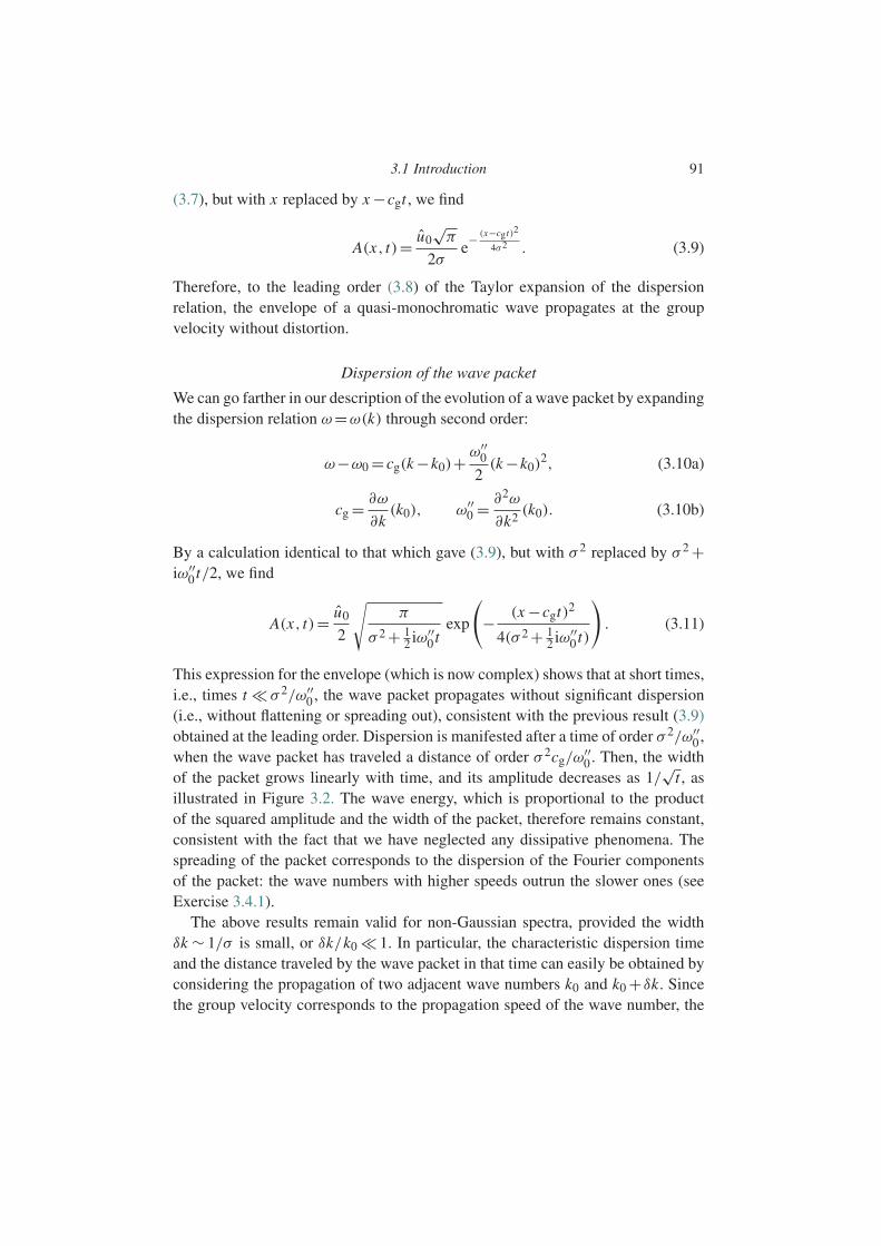
3.1 Introduction 91

(3.7), but with x replaced by x −cgt , we find

A(x, t)= u0√π

2σe− (x−cgt)2

4σ2 . (3.9)

Therefore, to the leading order (3.8) of the Taylor expansion of the dispersionrelation, the envelope of a quasi-monochromatic wave propagates at the groupvelocity without distortion.

Dispersion of the wave packet

We can go farther in our description of the evolution of a wave packet by expandingthe dispersion relation ω=ω(k) through second order:

ω−ω0 = cg(k −k0)+ω′′

0

2(k −k0)

2, (3.10a)

cg = ∂ω

∂k(k0), ω′′

0 = ∂2ω

∂k2(k0). (3.10b)

By a calculation identical to that which gave (3.9), but with σ 2 replaced by σ 2 +iω′′

0 t/2, we find

A(x, t)= u0

2

√π

σ 2 + 12 iω′′

0 texp

(− (x −cgt)2

4(σ 2 + 12 iω′′

0 t)

). (3.11)

This expression for the envelope (which is now complex) shows that at short times,i.e., times t σ 2/ω′′

0 , the wave packet propagates without significant dispersion(i.e., without flattening or spreading out), consistent with the previous result (3.9)obtained at the leading order. Dispersion is manifested after a time of order σ 2/ω′′

0 ,when the wave packet has traveled a distance of order σ 2cg/ω

′′0 . Then, the width

of the packet grows linearly with time, and its amplitude decreases as 1/√

t , asillustrated in Figure 3.2. The wave energy, which is proportional to the productof the squared amplitude and the width of the packet, therefore remains constant,consistent with the fact that we have neglected any dissipative phenomena. Thespreading of the packet corresponds to the dispersion of the Fourier componentsof the packet: the wave numbers with higher speeds outrun the slower ones (seeExercise 3.4.1).

The above results remain valid for non-Gaussian spectra, provided the widthδk ∼ 1/σ is small, or δk/k0 1. In particular, the characteristic dispersion timeand the distance traveled by the wave packet in that time can easily be obtained byconsidering the propagation of two adjacent wave numbers k0 and k0 +δk. Sincethe group velocity corresponds to the propagation speed of the wave number, the

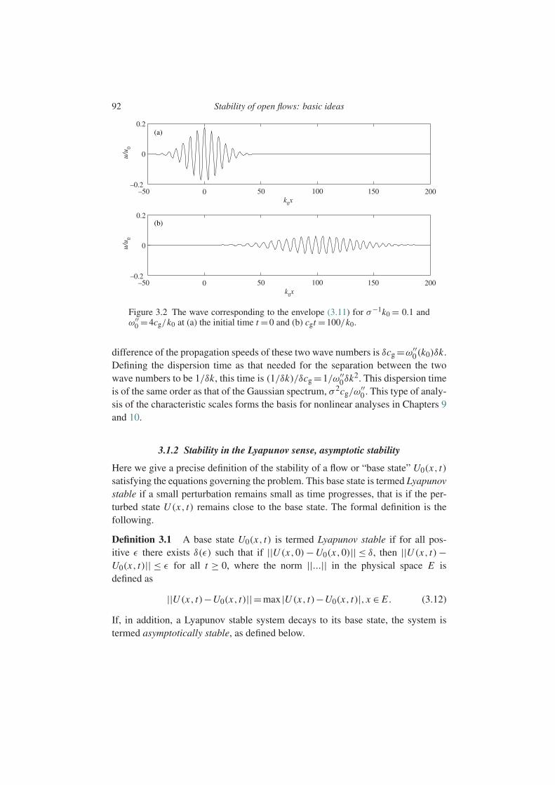
92 Stability of open flows: basic ideas

0.2

0

–0.2

0.2

0

–0.2

–50 0 50 100 150 200

–50 0 50 100 150 200k0x

k0x

u 0/u

u 0/u

(a)

(b)

Figure 3.2 The wave corresponding to the envelope (3.11) for σ−1k0 = 0.1 andω′′

0 =4cg/k0 at (a) the initial time t =0 and (b) cgt =100/k0.

difference of the propagation speeds of these two wave numbers is δcg =ω′′0(k0)δk.

Defining the dispersion time as that needed for the separation between the twowave numbers to be 1/δk, this time is (1/δk)/δcg =1/ω′′

0δk2. This dispersion timeis of the same order as that of the Gaussian spectrum, σ 2cg/ω

′′0 . This type of analy-

sis of the characteristic scales forms the basis for nonlinear analyses in Chapters 9and 10.

3.1.2 Stability in the Lyapunov sense, asymptotic stability

Here we give a precise definition of the stability of a flow or “base state” U0(x, t)satisfying the equations governing the problem. This base state is termed Lyapunovstable if a small perturbation remains small as time progresses, that is if the per-turbed state U (x, t) remains close to the base state. The formal definition is thefollowing.

Definition 3.1 A base state U0(x, t) is termed Lyapunov stable if for all pos-itive ε there exists δ(ε) such that if ||U (x,0)− U0(x,0)|| ≤ δ, then ||U (x, t)−U0(x, t)|| ≤ ε for all t ≥ 0, where the norm ||...|| in the physical space E isdefined as

||U (x, t)−U0(x, t)||=max |U (x, t)−U0(x, t)|, x ∈ E . (3.12)

If, in addition, a Lyapunov stable system decays to its base state, the system istermed asymptotically stable, as defined below.

3.1 Introduction 93

Definition 3.2 A base state U0(x, t) which is Lyapunov stable is termedasymptotically stable if there exists a δ such that if ||U (x,0)−U0(x,0)||≤ δ, then

limt→∞||U (x, t)−U0(x, t)||=0. (3.13)

The simplest example is the harmonic oscillator: without damping, it is Lya-punov stable, but not asymptotically stable; with damping, it is asymptoticallystable. However, except for elementary examples such as the harmonic oscillator,it is not possible to determine the stability of a particular base state by directlyverifying the above definitions! It is therefore essential to find stability criteria thatare easier to verify, and that is the goal of this chapter. The first step is to studythe linear stability, that is, the evolution of a perturbation given by the equationslinearized about the base state. The linearization procedure allows us to determinewhether the state is stable or unstable, provided the parameter values do not corre-spond to a bifurcation, as discussed in Chapter 1. Strictly speaking, the results of alinear stability analysis are valid only for perturbations of infinitesimal amplitude.In practice, the predictions of a linear stability analysis are generally valid for per-turbations of relative amplitude from 1% to 10%. Therefore, a linearly stable basestate is expected to be also Lyapunov stable.

A third stability definition, namely, that of global stability, is useful in the casewhere the flow returns to its base state for any perturbation amplitude, i.e., withoutregard for the magnitude of δ.

Definition 3.3 A base state U0(x, t) is globally stable if it is asymptotically sta-ble for arbitrary δ. In other words, the basin of attraction of the base flow coincideswith the entire phase space.

3.1.3 Linear stability and instability

We shall illustrate the ideas introduced in this chapter using the Ginzburg–Landauequation with real coefficients:

∂t u +V ∂x u = Ru +∂xx u −|u|2u, (3.14)

where u(x, t) is a complex scalar field and R and V are two parameters. Thisequation models the behavior of many physical systems (Cross and Hohenberg,1993). Here we need only note that the left-hand side of the equation has the struc-ture of a total derivative, implying an advection speed V , and that the right-handside contains a linear term involving the control parameter R, a diffusion term, anda nonlinear term. This equation has a base solution u0 =0 which is invariant undertranslations in x and t , as is the complete equation (3.14).

94 Stability of open flows: basic ideas

Linearizing (3.14) about the base state u0 = 0 (which here amounts simply toneglecting the nonlinear term |u|2u), we obtain the evolution equation for theperturbation which is written in operator form as

Lu(x, t)=0 with L = ∂t +V ∂x − R −∂xx . (3.15)

If the base state is perturbed by a given forcing function S(x, t), the perturbationevolves according to the equation

Lu(x, t)= S(x, t). (3.16)

Three elementary forcing functions are of special importance:

S(x, t)= F(x)δ(t), (3.17a)

S(x, t)= δ(x)δ(t), (3.17b)

S(x, t)= δ(x)H(t)e−iωt, (3.17c)

where δ and H are the Dirac and Heaviside functions, respectively. The first corre-sponds to a forcing with some spatial distribution applied at the instant t = 0, andthe problem then becomes an initial-value problem. The second corresponds to animpulse localized at x = 0 and t = 0; the solution is the “impulse response,” i.e.,the Green function G(x, t) associated with the linear operator L . The third forcingfunction corresponds to periodic forcing beginning at t =0 and localized at x =0.This type of forcing is often used in experiments, for example, when a small ribbonis made to vibrate at some point in a flow; examples are given in Chapters 5 and 6.Under typical experimental conditions the forcing can be modeled by a superposi-tion of two of the elementary forcing functions (3.17b) and (3.17c), or (3.17a) and(3.17c), with the initial forcing (3.17a) or (3.17b) corresponding to the start of theexperiment.

The definition of linear stability is based on the response to an impulse pertur-bation (3.17b). This perturbation can give rise to three types of behavior, which areillustrated in Figure 3.3. The perturbation advected by the flow can decay to zero(Figure 3.3a). The Green function then satisfies

limt→∞G(x, t)=0 along any ray x/t = constant. (3.18)

The base state u0 =0 is then termed linearly stable. Otherwise, it is termed linearlyunstable, i.e.,

limt→∞ G(x, t)=∞ along at least one ray x/t = constant. (3.19)

In the latter case two types of instability can be distinguished. The first, termedconvective, corresponds to a perturbation which, in addition to being amplified,

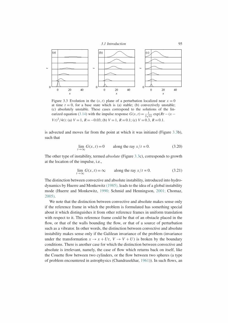
3.1 Introduction 95

0 20 400

x

t

(a)

0 20 400

xt

(b)

0 20 400

x

t

(c)

Figure 3.3 Evolution in the (x, t) plane of a perturbation localized near x = 0at time t = 0, for a base state which is (a) stable; (b) convectively unstable;(c) absolutely unstable. These cases correspond to the solutions of the lin-earized equation (3.14) with the impulse response G(x, t)= 1

2√π t

exp(Rt − (x −V t)2/4t): (a) V =1, R =−0.03; (b) V =1, R =0.1; (c) V =0.3, R =0.1.

is advected and moves far from the point at which it was initiated (Figure 3.3b),such that

limt→∞G(x, t)=0 along the ray x/t = 0. (3.20)

The other type of instability, termed absolute (Figure 3.3c), corresponds to growthat the location of the impulse, i.e.,

limt→∞ G(x, t)=∞ along the ray x/t = 0. (3.21)

The distinction between convective and absolute instability, introduced into hydro-dynamics by Huerre and Monkewitz (1985), leads to the idea of a global instabilitymode (Huerre and Monkewitz, 1990; Schmid and Henningson, 2001; Chomaz,2005).

We note that the distinction between convective and absolute makes sense onlyif the reference frame in which the problem is formulated has something specialabout it which distinguishes it from other reference frames in uniform translationwith respect to it. This reference frame could be that of an obstacle placed in theflow, or that of the walls bounding the flow, or that of a source of perturbationsuch as a vibrator. In other words, the distinction between convective and absoluteinstability makes sense only if the Galilean invariance of the problem (invarianceunder the transformation x → x +Ut , V → V +U ) is broken by the boundaryconditions. There is another case for which the distinction between convective andabsolute is irrelevant, namely, the case of flow which returns back on itself, likethe Couette flow between two cylinders, or the flow between two spheres (a typeof problem encountered in astrophysics (Chandrasekhar, 1961)). In such flows, an

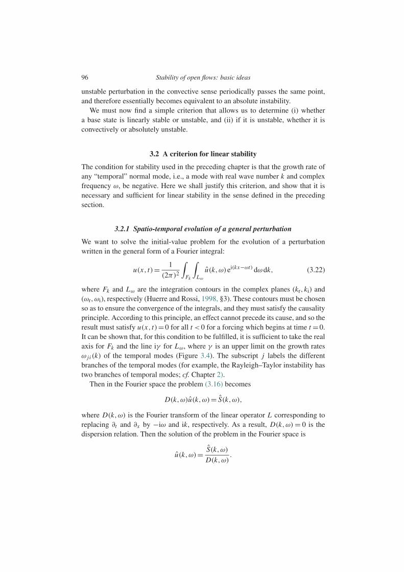
96 Stability of open flows: basic ideas

unstable perturbation in the convective sense periodically passes the same point,and therefore essentially becomes equivalent to an absolute instability.

We must now find a simple criterion that allows us to determine (i) whethera base state is linearly stable or unstable, and (ii) if it is unstable, whether it isconvectively or absolutely unstable.

3.2 A criterion for linear stability

The condition for stability used in the preceding chapter is that the growth rate ofany “temporal” normal mode, i.e., a mode with real wave number k and complexfrequency ω, be negative. Here we shall justify this criterion, and show that it isnecessary and sufficient for linear stability in the sense defined in the precedingsection.

3.2.1 Spatio-temporal evolution of a general perturbation

We want to solve the initial-value problem for the evolution of a perturbationwritten in the general form of a Fourier integral:

u(x, t)= 1

(2π)2

∫Fk

∫Lω

u(k,ω)ei(kx−ωt) dωdk, (3.22)

where Fk and Lω are the integration contours in the complex planes (kr,ki) and(ωr,ωi), respectively (Huerre and Rossi, 1998, §3). These contours must be chosenso as to ensure the convergence of the integrals, and they must satisfy the causalityprinciple. According to this principle, an effect cannot precede its cause, and so theresult must satisfy u(x, t)=0 for all t <0 for a forcing which begins at time t =0.It can be shown that, for this condition to be fulfilled, it is sufficient to take the realaxis for Fk and the line iγ for Lω, where γ is an upper limit on the growth ratesω j i (k) of the temporal modes (Figure 3.4). The subscript j labels the differentbranches of the temporal modes (for example, the Rayleigh–Taylor instability hastwo branches of temporal modes; cf. Chapter 2).

Then in the Fourier space the problem (3.16) becomes

D(k,ω)u(k,ω)= S(k,ω),

where D(k,ω) is the Fourier transform of the linear operator L corresponding toreplacing ∂t and ∂x by −iω and ik, respectively. As a result, D(k,ω) = 0 is thedispersion relation. Then the solution of the problem in the Fourier space is

u(k,ω)= S(k,ω)

D(k,ω).

3.2 A criterion for linear stability 97

ki

Fk

ωi

ω1(k) ω2(k) ω3(k)

ωr

Lω

kr

Figure 3.4 Integration contours Fk and Lω in the (kr,ki) and (ωr,ωi) planes assur-ing the convergence of the integral (3.22) as well as the causality principle. Theω j (k) are the temporal branches.

Insertion of this result into (3.22) formally solves the problem in physical space:

u(x, t)= 1

(2π)2

∫Fk

∫Lω

S(k,ω)

D(k,ω)ei(kx−ωt) dωdk. (3.23)

This integral is dominated by the poles of the integrand, that is, the zeros ofD(k,ω). Since the integration contour Fk is the real axis, these zeros correspondto the temporal modes ω j (k). If the poles are simple, the residue theorem3 can beused to write the solution as

u(x, t)=− i

2π j

∫ ∞

−∞S(k,ω j (k))

∂ωD(k,ω j (k))ei(kx−ω j (k)t) dk. (3.24)

Therefore, the response to the forcing S(x, t) is, in the end, a sum of temporalnormal modes. A necessary and sufficient condition for stability then is that thegrowth rates, that is, the imaginary parts of the ω j (k), are negative for all j andany wave number k. In conclusion, the stability criterion defined at the beginningof the present chapter and based on the response to a localized perturbation isidentical to the criterion used in the preceding chapter based only on the temporalmodes.

3 We recall that a function f (z) of a complex variable z is holomorphic in a domain D if it is uniform (single-valued) and differentiable at any point of D. A pole a is a point where f (z), being uniform, is neither boundednor holomorphic, but where 1

f (z) is holomorphic (an example is 1z−a ). The residue associated with a pole a

is the coefficient A−1 of the term 1z−a of the expansion of f (z) in negative or positive powers of (z −a) (a

Laurent series). Let L be an integration contour in the complex plane for a function f (z) which is holomorphic

inside L , except at n poles with residues A( j)−1, j =1,n. Then∫L

f (z)dz =2iπ∑

j

A( j)−1.

This is the residue theorem. (The theorem remains valid if 1/ f (z) is not holomorphic at the points a j , i.e., foressential singularities.)

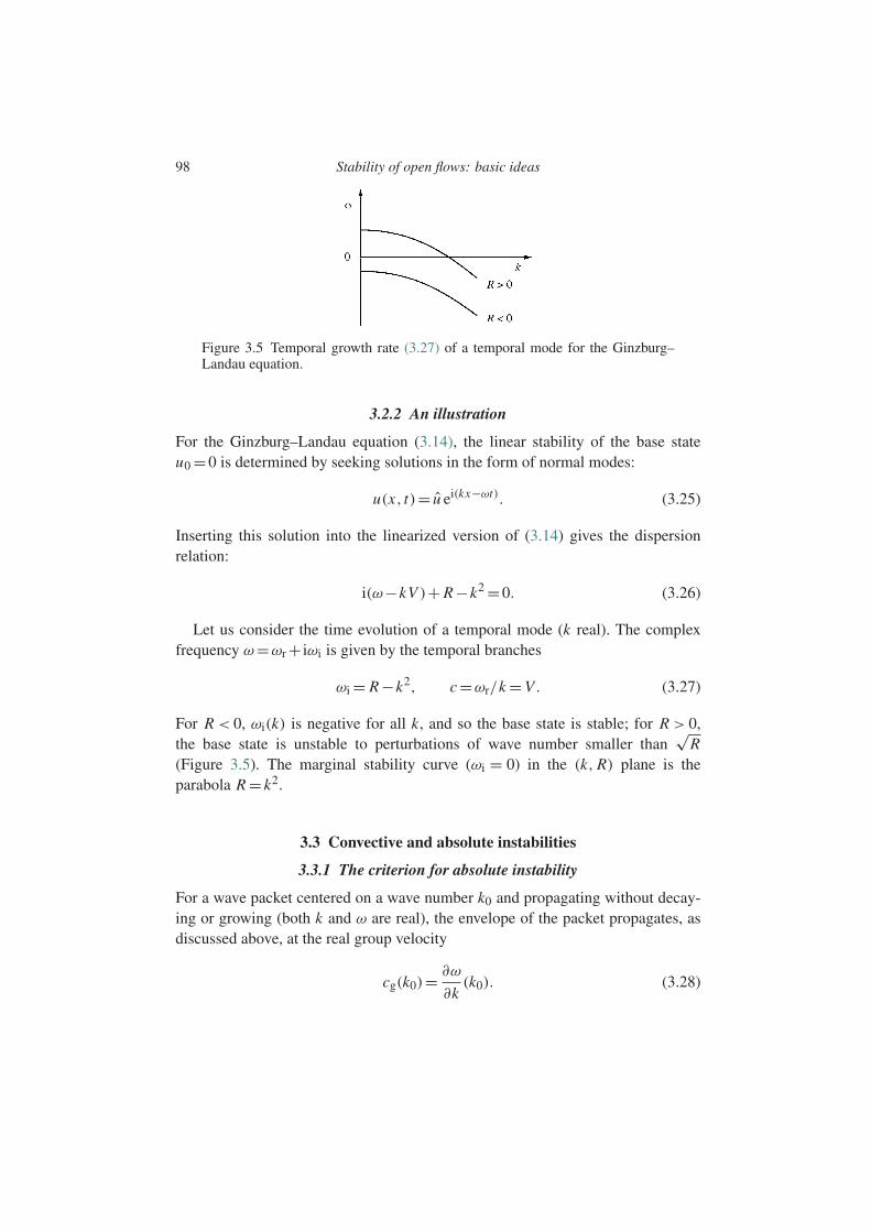
98 Stability of open flows: basic ideas

Figure 3.5 Temporal growth rate (3.27) of a temporal mode for the Ginzburg–Landau equation.

3.2.2 An illustration

For the Ginzburg–Landau equation (3.14), the linear stability of the base stateu0 =0 is determined by seeking solutions in the form of normal modes:

u(x, t)= u ei(kx−ωt). (3.25)

Inserting this solution into the linearized version of (3.14) gives the dispersionrelation:

i(ω−kV )+ R −k2 =0. (3.26)

Let us consider the time evolution of a temporal mode (k real). The complexfrequency ω=ωr + iωi is given by the temporal branches

ωi = R −k2, c =ωr/k = V . (3.27)

For R < 0, ωi(k) is negative for all k, and so the base state is stable; for R > 0,the base state is unstable to perturbations of wave number smaller than

√R

(Figure 3.5). The marginal stability curve (ωi = 0) in the (k, R) plane is theparabola R = k2.

3.3 Convective and absolute instabilities

3.3.1 The criterion for absolute instability

For a wave packet centered on a wave number k0 and propagating without decay-ing or growing (both k and ω are real), the envelope of the packet propagates, asdiscussed above, at the real group velocity

cg(k0)= ∂ω

∂k(k0). (3.28)

3.3 Convective and absolute instabilities 99

Let us now see what happens in the neighborhood of an instability threshold (withk and ω complex) for a value of the bifurcation parameter R close to the criticalvalue Rc (Huerre and Rossi, 1998, §3). At the threshold R = Rc the curve describ-ing the growth rate ωi(kr) of the temporal normal modes is tangent to the axiskr at real critical wave number kc, and so ∂ωi/∂kr is necessarily zero. The groupvelocity of a wave packet centered on the critical wave number kc,

cg(kc)= ∂ω

∂k(kc, Rc)= ∂ωr

∂kr= ∂ωi

∂ki, (3.29)

is indeed real.4

Above the threshold, if there exists a wave number k0 for which the groupvelocity cg(k0) is zero and the temporal growth rate (i.e., the imaginary part ofω0 =ω(k0)) is positive, then the packet grows in place (Figure 3.3c). This resultis obtained by calculating the impulse response G(x, t) along the ray x/t = 0,given by (3.24) with S(k,ω)= 1 inside the integral. The integral is calculated bygeneralizing the stationary-phase method to the case where the argument of theexponential is not purely imaginary, but contains a real part (Bender and Orszag,1978, §6.6). The resulting asymptotic response at long times is given by

G(x, t)∼ 1√2πω′′(k0)t

eiπ/4

∂ωD(k0,ω0)ei(k0x−ω0t), (3.30)

where k0 and ω0 are defined through

∂ω

∂k(k0)=0, ω0 =ω(k0). (3.31)

It follows that the instability criterion is simply that the imaginary part of ω0,referred to as the absolute growth rate, be positive.

From this discussion we can deduce an essential characteristic of convective andabsolute instabilities. A convective instability amplifies any unstable perturbation,and advects it downstream. If the perturbations are viewed as “noise,” an unstableconvective system then behaves as a noise amplifier. On the other hand, a systemwhich is absolutely unstable responds selectively to perturbations: its response is

4 For a function Z = X +iY of a complex variable z = x +iy to be differentiable at the point z0, it is necessary andsufficient that X (x, y) and Y (x, y) be differentiable at (x0, y0) and that at this point (the Cauchy conditions)

∂X

∂x= ∂Y

∂y,

∂X

∂y=− ∂Y

∂x.

The derivative Z ′ is then given by

Re(Z ′)= ∂X

∂x= ∂Y

∂y, Im(Z ′)=− ∂X

∂y= ∂Y

∂x.

100 Stability of open flows: basic ideas

dominated by the mode with zero group velocity, which grows in place, whilethe other modes are “swept away” by the flow. Since this mode is selected by thedispersion relation, which is intrinsic to the system, an absolutely unstable systembehaves like an oscillator with its own natural frequency.

3.3.2 The spatial branches of a convective instability

Let us consider the situation shown in Figure 3.3b of a perturbation with givenfrequency advected by a flow. We want to determine the spatial growth rate of thisperturbation. This problem makes sense only in the case of a convective instability,because for an absolute instability the perturbation field is dominated by the modewith zero group velocity, which grows in place. The spatial growth rate is obtainedby using the dispersion relation D(k,ω)=0 to find the spatial branches, that is, thecomplex wave number(s) kr + iki corresponding to a real frequency ω. The spatialgrowth rate is then −ki and the speed of the wave is ω/kr.

3.3.3 Illustrations

As a simple example, let us consider the Ginzburg–Landau equation, for which thedispersion relation is (3.26). The (complex) group velocity of a wave number k isthen

cg = ∂ω

∂k= V −2ik, (3.32)

which vanishes for wave number k0 = V/2i. Inserting this wave number into thedispersion relation (3.26), we find the corresponding frequency ω0 = i(R −V 2/4).We conclude that for 0< R < V 2/4 the base state u0 = 0 is convectively unstable(Figure 3.3b), and that for R > V 2/4 it is absolutely unstable (Figure 3.3c).

When the instability is convective, i.e., R < V 2/4, the two spatial branches (orspatial modes) are obtained from (3.26):

k±(ω)= 1

2

(−iV ±

√4(R + iω)−V 2

), (3.33)

from which we easily obtain the spatial growth rate −k±,i. We stress the fact thatthe spatial branches can be determined only when we are sure that the instabilityis convective.

We briefly mention some hydrodynamical illustrations which will be treated inmore detail later on. The mixing layer between two concurrent and parallel flowswith different velocities is a typical example of a flow which is convectively unsta-ble. The Poiseuille flow between flat plates or in a pipe, as well as the boundary

3.3 Convective and absolute instabilities 101

layer on a flat plate, are two other important examples. In such flows, any per-turbation which is forced at an upstream location is amplified downstream; theinstability does not have its own dynamics. On the other hand, the wake down-stream from a solid obstacle is absolutely unstable beyond a critical Reynoldsnumber of a few tens. For example, Rec =U∞d/ν=48.5 for a cylinder of diameterd in a flow of unperturbed velocity U∞. At this critical Reynolds number the flowbifurcates from a stationary state to an oscillatory state characterized physicallyby the appearance of a Karman vortex street (Williamson, 1996; Huerre and Rossi,1998, §6). The oscillation frequency f corresponds to a well-defined value of theStrouhal number f d/U∞, which is quite insensitive to perturbations of the flow(St = 0.19 for the cylinder at moderate Reynolds numbers). In terms of dynamicalsystems, the appearance of this oscillation corresponds to a Hopf bifurcation.

3.3.4 The Gaster relation

The Gaster relation (1962) is an expression allowing the temporal growth rate tobe related to the spatial growth rate in the vicinity of marginal stability. Let usconsider a marginal normal mode (kc,ωc) such that ωci =0 and kci =0. Expandingthe dispersion relation ω(k) in a Taylor series in the neighborhood of the marginalstability, to first order we have

ω−ωc = ∂ω

∂k(kc, R)(k −kc),

from which, taking the imaginary part, we find

ωi = ∂ωi

∂kr(kc, R)(kr −kc)+ ∂ωr

∂kr(kc, R)ki. (3.34)

For a temporal mode, ki is zero and the above relation gives the temporal growthrate ω

(T)i :

ω(T)i = ∂ωi

∂kr(kc, R)(kr −kc).

For a spatial mode, ωi is zero and (3.34) gives the spatial growth rate −k(S)i :

0= ∂ωi

∂kr(kc, R)(kr −kc)+ ∂ωr

∂kr(kc, R)k(S)

i .

Subtracting these two equations from each other and using cg = ∂ωr/∂kr, we find

ω(T)i =−cgk(S)

i . (3.35)

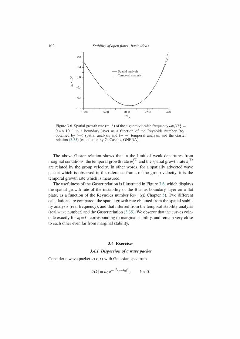
102 Stability of open flows: basic ideas

1000 1400 1800Reδ1

k i ×

102

Spatial analysisTemporal analysis

2200 2600–1.2

–0.8

–0.4

0.0

0.4

0.8

Figure 3.6 Spatial growth rate (m−1) of the eigenmode with frequency ων/U 2∞ =0.4 × 10−4 in a boundary layer as a function of the Reynolds number Reδ1obtained by (—) spatial analysis and (− −) temporal analysis and the Gasterrelation (3.35) (calculation by G. Casalis, ONERA).

The above Gaster relation shows that in the limit of weak departures frommarginal conditions, the temporal growth rate ω

(T)i and the spatial growth rate k(S)

iare related by the group velocity. In other words, for a spatially advected wavepacket which is observed in the reference frame of the group velocity, it is thetemporal growth rate which is measured.

The usefulness of the Gaster relation is illustrated in Figure 3.6, which displaysthe spatial growth rate of the instability of the Blasius boundary layer on a flatplate, as a function of the Reynolds number Reδ1 (cf. Chapter 5). Two differentcalculations are compared: the spatial growth rate obtained from the spatial stabil-ity analysis (real frequency), and that inferred from the temporal stability analysis(real wave number) and the Gaster relation (3.35). We observe that the curves coin-cide exactly for ki = 0, corresponding to marginal stability, and remain very closeto each other even far from marginal stability.

3.4 Exercises

3.4.1 Dispersion of a wave packet

Consider a wave packet u(x, t) with Gaussian spectrum

u(k)= u0 e−σ 2(k−k0)2, k >0.

3.4 Exercises 103

1. Show that u(x, t) is given at long times (t 1 with =ω′′0/2σ 2) by

u(x, t)∼ u0√π

2σ

1√t

e− (x−cgt)2

(2σt)2 cos[k0x −ω0t +φ(x, t)],

where the phase φ(x, t) is defined as

φ(x, t)=−θ

2+ (x −cgt)2

4σ 2t, tanθ =t .

2. Show that the local wave number (the gradient of the phase) varies spatially as

∂xφ(x, t)= x −cgt

ω′′0 t

.

Interpret this variation.3. For gravity waves in deep water and δk = 0.1k0, at what distance from the

amplitude maximum are the wave numbers k0 ±δk found?

3.4.2 Spatial branches of a convective instability

Determine the spatial growth rate (3.33) of perturbations of the solution u(x, t)=0 of the Ginzburg–Landau equation (3.14) when the instability is convective(R < V 2/4).

4

Inviscid instability of parallel flows

4.1 Introduction

An instability typical of a parallel flow was demonstrated in an experimentperformed by Osborne Reynolds (1883) and repeated by Thorpe (1969). A hor-izontal long tube is filled carefully with a layer of water lying on top of a layerof heavier colored brine (salt water), as sketched in Figure 4.1a. The tube is sud-denly tipped several degrees: the brine falls and the water rises, creating a shearflow which displays an inflection point near the interface (Figure 4.1b). In a fewseconds a wave of sinusoidal shape develops at the interface of the two fluids, andleads to regular co-rotating vortices, as shown in Figure 4.2. These vortices are amanifestation of the Kelvin–Helmholtz instability. This instability owes its originto the inertia of the fluids; viscosity plays only a minor role, tending to attenuatethe growth of the wave only slightly by momentum diffusion.

Another manifestation of the Kelvin–Helmholtz instability on a much largeratmospheric scale is illustrated in Figure 4.3. An upper air layer flows over a lowerlayer moving more slowly, with different humidity and temperature. The thin layerof clouds formed at the interface displays billows which are the exact analogs ofthose in Figure 4.1. Figure 4.4 shows another example, in a mixing layer formedbetween a flow of water on the left and a flow of water and air bubbles on the right.

The parallel flow of two fluid layers moving at different speeds, as in the aboveexamples, is a typical situation manifesting the Kelvin–Helmholtz instability. A jetis a situation of the same type, as shown in Figure 4.5. This figure shows carbondioxide jetting into air as observed by shadowgraphy. The laminar jet emerg-ing from the nozzle is convectively unstable. The instability grows spatially andbecomes apparent at a distance of the order of a diameter, where it develops annu-lar vortices. These vortices in turn become unstable at a distance of the order of twowavelengths. This secondary instability leads to intense turbulent mixing betweenthe jet and the surrounding air.

104

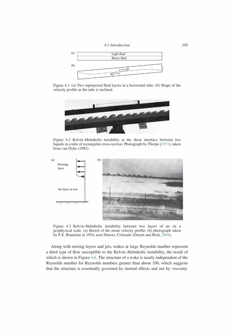
4.1 Introduction 105

Light fluid(a)

(b)

Heavy fluid

Figure 4.1 (a) Two superposed fluid layers in a horizontal tube. (b) Shape of thevelocity profile as the tube is inclined.

Figure 4.2 Kelvin–Helmholtz instability at the shear interface between twoliquids in a tube of rectangular cross-section. Photograph by Thorpe (1971), takenfrom van Dyke (1982).

(b)(a)

Flowinglayer

Air layer at rest

Figure 4.3 Kelvin–Helmholtz instability between two layers of air on ageophysical scale. (a) Sketch of the mean velocity profile; (b) photograph takenby P. E. Branstine in 1954, near Denver, Colorado (Drazin and Reid, 2004).

Along with mixing layers and jets, wakes at large Reynolds number representa third type of flow susceptible to the Kelvin–Helmholtz instability, the result ofwhich is shown in Figure 4.6. The structure of a wake is nearly independent of theReynolds number for Reynolds numbers greater than about 100, which suggeststhat the structure is essentially governed by inertial effects and not by viscosity.

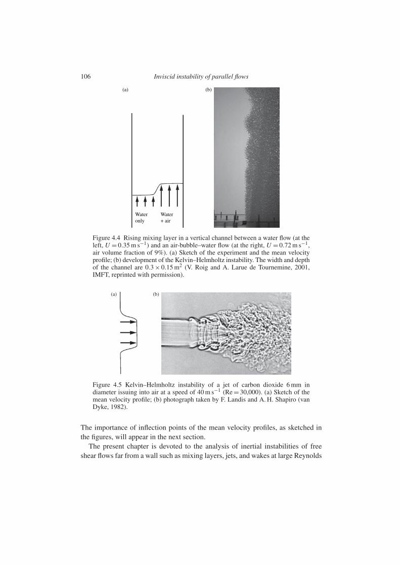
106 Inviscid instability of parallel flows

(b)(a)

Wateronly

Water+ air

Figure 4.4 Rising mixing layer in a vertical channel between a water flow (at theleft, U = 0.35 m s−1) and an air-bubble–water flow (at the right, U = 0.72 m s−1,air volume fraction of 9%). (a) Sketch of the experiment and the mean velocityprofile; (b) development of the Kelvin–Helmholtz instability. The width and depthof the channel are 0.3 × 0.15 m2 (V. Roig and A. Larue de Tournemine, 2001,IMFT, reprinted with permission).

(b)(a)

Figure 4.5 Kelvin–Helmholtz instability of a jet of carbon dioxide 6 mm indiameter issuing into air at a speed of 40 m s−1 (Re = 30,000). (a) Sketch of themean velocity profile; (b) photograph taken by F. Landis and A. H. Shapiro (vanDyke, 1982).

The importance of inflection points of the mean velocity profiles, as sketched inthe figures, will appear in the next section.

The present chapter is devoted to the analysis of inertial instabilities of freeshear flows far from a wall such as mixing layers, jets, and wakes at large Reynolds

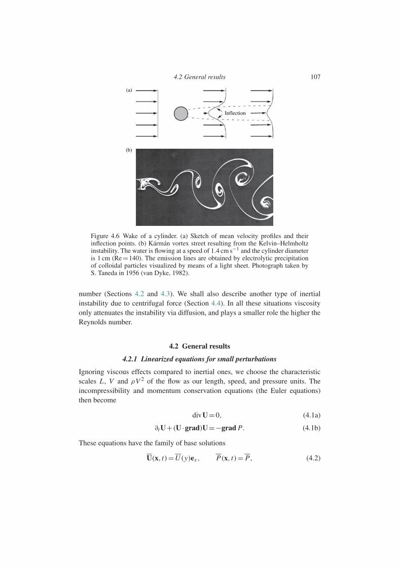
4.2 General results 107

Inflection

(a)

(b)

Figure 4.6 Wake of a cylinder. (a) Sketch of mean velocity profiles and theirinflection points. (b) Karman vortex street resulting from the Kelvin–Helmholtzinstability. The water is flowing at a speed of 1.4 cm s−1 and the cylinder diameteris 1 cm (Re =140). The emission lines are obtained by electrolytic precipitationof colloidal particles visualized by means of a light sheet. Photograph taken byS. Taneda in 1956 (van Dyke, 1982).

number (Sections 4.2 and 4.3). We shall also describe another type of inertialinstability due to centrifugal force (Section 4.4). In all these situations viscosityonly attenuates the instability via diffusion, and plays a smaller role the higher theReynolds number.

4.2 General results

4.2.1 Linearized equations for small perturbations

Ignoring viscous effects compared to inertial ones, we choose the characteristicscales L , V and ρV 2 of the flow as our length, speed, and pressure units. Theincompressibility and momentum conservation equations (the Euler equations)then become

divU=0, (4.1a)

∂t U+(U ·grad)U=−grad P. (4.1b)

These equations have the family of base solutions

U(x, t)=U (y)ex , P(x, t)= P, (4.2)

108 Inviscid instability of parallel flows

corresponding to a parallel flow in the x-direction specified by the unit vector ex ,invariant in the spanwise z-direction. Let us consider the perturbed base flow U+u,P + p; the linearized perturbation equations are written as

divu=0, (4.3a)

(∂t +U∂x )u+v∂yU ex =−grad p. (4.3b)

Since the problem is translationally invariant in time and in the spatial directionsx and z, the solution can be sought in the form of normal modes of wave vector k=kx ex +kzez and frequency ω. For the longitudinal velocity perturbation a normalmode is written as

u(x, t)= 1

2u(y)ei(kx x+kz z−ωt)+c.c., (4.4)

with similar expressions for v, w and p. Substituting these into (4.3), we obtainthe system of homogeneous differential equations satisfied by the amplitudes u(y),v(y), w(y), and p(y):

ikx u +∂y v+ ikzw=0, (4.5a)

i(kxU −ω)u +∂yU v=−ikx p, (4.5b)

i(kxU −ω)v=−∂y p, (4.5c)

i(kxU −ω)w=−ikz p. (4.5d)

In addition to the equations (4.5), we impose the conditions that the perturbationsfall off for y →±∞:

u, v, w→0 for y →±∞, (4.6)

or, for bounded domains, that walls located at y = y1 and y = y2 are imperme-able, i.e.

v(y1)=0, v(y2)=0. (4.7)

The system (4.5)–(4.6) or (4.5)–(4.7) can formally be written as

Lφ=ωMφ,

where φ= (u, v, w, p) and L and M are linear differential operators.We recognize this as a generalized eigenvalue problem which has a nonzero

solution φ only if the operator L −ωM is noninvertible, i.e., if for a given wavenumber the frequency ω is an eigenvalue. This condition can be written formally as

D(k,ω)=0, (4.8)

4.2 General results 109

which is the dispersion relation of perturbations of infinitesimal amplitude. Obtain-ing the explicit dispersion relation for a specific base flow is the essentialcomponent of a linear stability study. The rest of this chapter is devoted to thedescription of some general results on inviscid shear flows.

4.2.2 The Squire theorem

Using a change of variable and a theorem due to Squire (1933), the three-dimensional problem (4.5)–(4.6) or (4.5)–(4.7) can be reduced to an equivalenttwo-dimensional one. The Squire transformation consists of introducing thevariables

k2 = k2x +k2

z , (4.9a)

ω= (k/kx )ω, (4.9b)

ku = kx u +kzw, (4.9c)

v= v, (4.9d)

p = (k/kx ) p. (4.9e)

The system (4.5) then becomes

iku +∂y v=0, (4.10a)

ik(U − c)u +∂yU v=−ik p, (4.10b)

ik(U − c)v=−∂y p, (4.10c)

where c = c = ω/kx is the phase velocity of the perturbation in the direction x ,with the boundary conditions

v(y)→0 for y →±∞, or v(y1)= v(y2)=0. (4.11)

The resulting system of equations (4.10)–(4.11) is formally identical to the origi-nal system (4.5)–(4.6) or (4.5)–(4.7) with w= kz = 0; in other words, the systemobtained after the Squire transformation is identical to that corresponding to two-dimensional perturbations. This system of two-dimensional perturbations has anonzero solution only if the dispersion relation

D(k, ω)=0 (4.12)

is satisfied. If this relation is known, i.e., if we have managed to solve the stabilityproblem for two-dimensional perturbations, the dispersion relation (4.8) for three-dimensional perturbations can be obtained without further calculation by means of

110 Inviscid instability of parallel flows

the Squire transformation:

D(k,ω)= D

√k2x +k2

z ,

√k2

x +k2z

kxω

=0. (4.13)

This leads us to Squire’s theorem.

Theorem 4.1 For any three-dimensional unstable mode (k,ω) of temporalgrowth rate ωi there is an associated two-dimensional mode (k, ω) of temporal

growth rate ωi =ωi

√k2

x +k2z /kx , which is more unstable since ωi >ωi .

Therefore, when the problem is to determine an instability condition, it issufficient to consider only two-dimensional perturbations.

4.2.3 The Rayleigh equation of two-dimensional perturbations

With Squire’s theorem in mind, we shall henceforth consider only two-dimensionalperturbations. Then we can introduce the stream function ψ of the velocityperturbation, defined as u = ∂yψ and v = −∂yψ . Eliminating the pressure bycross-differentiation of the Euler equations, we obtain

(∂t +U∂x )ψ −∂yyU ∂xψ =0. (4.14)

(It may be noted that this equation is simply the linearized transport equation forthe vorticity ω=−ψez in the absence of diffusion.) Seeking the solution in theform of normal modes

ψ(x, t)= 1

2ψ(y)ei(kx−ωt)+c.c.

of wave vector k= kex and frequency ω, we obtain the Rayleigh equation

(U −c)(∂yyψ −k2ψ)−∂yyU ψ =0 (4.15)

with the boundary conditions

ψ →0 for y →±∞, or ψ(y1)= ψ(y2)=0. (4.16)

In light of the results obtained in the preceding chapter, to determine the stabilityof a flow it is sufficient to consider modes with real wave number. For such a mode,if ψ is an eigenfunction associated with an eigenvalue c, then, if we consider thecomplex conjugate version of the Rayleigh equation, we see that ψ∗ is also aneigenfunction associated with the eigenvalue c∗. The eigenvalues associated withthe Rayleigh equation must therefore be either real or complex conjugates of each

4.2 General results 111

other. If the eigenvalues are real for any wave number, the perturbations are waveswhich propagate without amplification, and the flow is neutrally stable. If thereexists a wave number for which the two eigenvalues are complex conjugates ofeach other, one of the modes decays and the other is amplified, and so the flow isunstable.

A result which will prove useful for what follows is that if the flow is stable withrespect to a normal mode (ci =0), then the corresponding perturbations u and v areexactly out of phase. Here the Rayleigh equation has real coefficients, and the realand imaginary parts of ψ satisfy the same linear equation: they are proportional,and so their ratio is independent of y. The phase φ of ψ(y)= A(y)eiφ(y) is thereforeindependent of y, and the perturbations u and v may be written as

u = A′(y)cos(kx −ωt +φ), v= k A(y)sin(kx −ωt +φ),

which proves that they are out of phase.

The critical layer

A complication can arise in solving the Rayleigh equation if there exists a layer inthe flow, at some location y = yc, where the speed c of an eigenmode is equal to thefluid velocity U (yc): the coefficient of the highest-order differential in the Rayleighequation (4.15) vanishes. The eigenfunction therefore must have a singularity aty = yc (at least, it is not differentiable there). Such a layer is called a critical layer.Since the speed c =U (yc) is real, the stability of such a mode must be neutral.

It may be remarked in general that the factor U (y) − c can vanish for acomplex value of the variable y, as the associated eigenvalue is no longer real.Such a situation may seem to have no physical consequence because the spatialvariable y is real, but in fact it can have an important effect on the structure of theeigenfunctions. For a deeper discussion of this point see in particular the studiesof Lin (1955), Bender and Orszag (1978, §3.1–3.3), Drazin and Reid (2004, §22),Huerre and Rossi (1998), or Schmid and Henningson (2001, §2.2).

The continuous spectrum

If, for a given wave number, there exists a mode associated with a critical layer aty = yc near which the velocity U (y) is continuous, one might think that there mustexist other neutral eigenmodes with speed c = U (y) in a range about y = yc; theeigenvalue spectrum associated with these modes is then continuous. The case ofCouette flow discussed below offers a simple illustration of this type of spectrum.We note that the continuity we are discussing here concerns an ensemble of modesof the same wave number; it is different than that of a Fourier spectrum where thewave number is continuous.

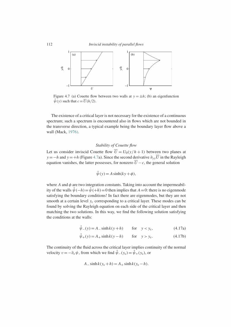
112 Inviscid instability of parallel flows

1(a) (b)

0

–1U ψ

y/h

1

0

–1

y/h

Figure 4.7 (a) Couette flow between two walls at y = ±h; (b) an eigenfunctionψ(y) such that c =U (h/2).

The existence of a critical layer is not necessary for the existence of a continuousspectrum; such a spectrum is encountered also in flows which are not bounded inthe transverse direction, a typical example being the boundary layer flow above awall (Mack, 1976).

Stability of Couette flow

Let us consider inviscid Couette flow U = U0(y/h + 1) between two planes aty =−h and y =+h (Figure 4.7a). Since the second derivative ∂yyU in the Rayleighequation vanishes, the latter possesses, for nonzero U −c, the general solution

ψ(y)= A sinh(ky +φ),

where A and φ are two integration constants. Taking into account the impermeabil-ity of the walls ψ(−h)= ψ(+h)=0 then implies that A=0: there is no eigenmodesatisfying the boundary conditions! In fact there are eigenmodes, but they are notsmooth at a certain level yc corresponding to a critical layer. These modes can befound by solving the Rayleigh equation on each side of the critical layer and thenmatching the two solutions. In this way, we find the following solution satisfyingthe conditions at the walls:

ψ−(y)= A− sinhk(y +h) for y < yc, (4.17a)

ψ+(y)= A+ sinhk(y −h) for y > yc. (4.17b)

The continuity of the fluid across the critical layer implies continuity of the normalvelocity v=−∂xψ , from which we find ψ−(yc)= ψ+(yc), or

A− sinhk(yc +h)= A+ sinhk(yc −h).

4.2 General results 113

This equation determines a continuous family of eigenfunctions, parametrized byyc in the interval [y1, y2] (up to a multiplicative constant, since as usual, the prob-lem is linear and homogeneous). The eigenfunction with yc =h/2 associated withthe eigenvalue c =U (h/2) is shown in Figure 4.7b: it is continuous at y = yc butnot differentiable. Physically, the discontinuity of the derivative corresponds to adiscontinuity of the longitudinal velocity u =∂yψ , which is entirely admissible forinviscid flow.

Therefore, for inviscid Couette flow, any normal mode of wave number k andspeed c=ω/k in the range between U (−h)=0 and U (+h)=2U0 is an eigenmode.The dispersion relation can then be written as

kU (−h)<ω< kU (+h).

In other words, for any wave number k the eigenvalue spectrum ω(k) is continuous.It can be concluded that the discrete spectrum of inviscid Couette flow is empty, butthere exists a continuous spectrum associated with the neutral modes. This flow istherefore linearly stable (Case, 1960). As will be shown in the following chapter,the inclusion of viscous effects does not modify this result: as a consequence,Couette flow is linearly stable for any Reynolds number (Romanov, 1973).

4.2.4 The Rayleigh inflection point theorem

Inviscid modes of instability are governed by the Rayleigh equation (4.15). It is ofsome interest to establish general properties of solutions to this equation withoutactually solving it for specific velocity profiles. The Rayleigh theorem (1880) isone such general result, which establishes conditions of far-reaching consequence.

The Rayleigh theorem. The existence of an inflection point in the velocity profileof a parallel flow is a necessary (but not sufficient) condition for instability.

Let us prove this theorem. According to the results of the preceding chapter, itis sufficient to study the temporal stability for determining the stability of a givenflow, i.e., it is sufficient to consider modes with real wave number and complexfrequency. Let us assume that the flow is unstable. Then ci = 0 and U − c = 0for real y. We divide the Rayleigh equation (4.15) by (U − c), multiply by ψ∗,and integrate between the walls at y1 and y2. After integrating by parts takinginto account the conditions ψ(y1)= ψ(y2)= 0, the imaginary part of the result iswritten as

ci

∫ y2

y1

∂yyU

|U −c|2 |ψ |2dy =0. (4.18)

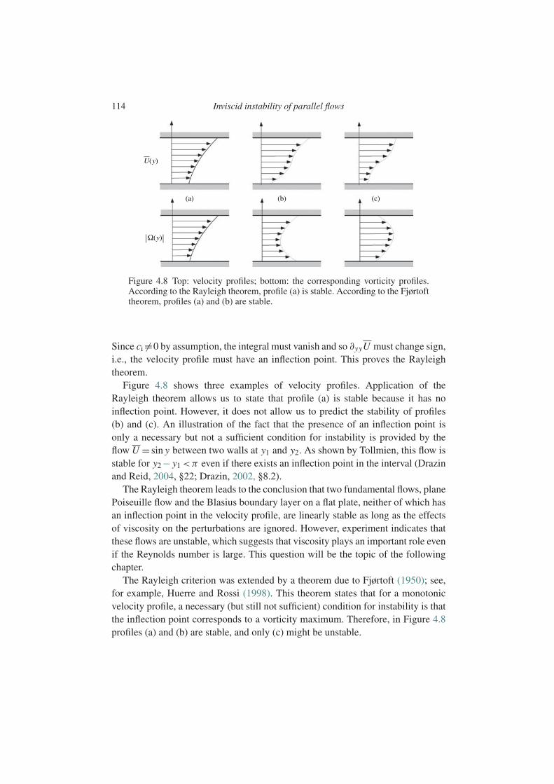
114 Inviscid instability of parallel flows

(a)

U(y)

Ω(y)

(b) (c)

Figure 4.8 Top: velocity profiles; bottom: the corresponding vorticity profiles.According to the Rayleigh theorem, profile (a) is stable. According to the Fjørtofttheorem, profiles (a) and (b) are stable.

Since ci =0 by assumption, the integral must vanish and so ∂yyU must change sign,i.e., the velocity profile must have an inflection point. This proves the Rayleightheorem.

Figure 4.8 shows three examples of velocity profiles. Application of theRayleigh theorem allows us to state that profile (a) is stable because it has noinflection point. However, it does not allow us to predict the stability of profiles(b) and (c). An illustration of the fact that the presence of an inflection point isonly a necessary but not a sufficient condition for instability is provided by theflow U = sin y between two walls at y1 and y2. As shown by Tollmien, this flow isstable for y2 − y1 <π even if there exists an inflection point in the interval (Drazinand Reid, 2004, §22; Drazin, 2002, §8.2).

The Rayleigh theorem leads to the conclusion that two fundamental flows, planePoiseuille flow and the Blasius boundary layer on a flat plate, neither of which hasan inflection point in the velocity profile, are linearly stable as long as the effectsof viscosity on the perturbations are ignored. However, experiment indicates thatthese flows are unstable, which suggests that viscosity plays an important role evenif the Reynolds number is large. This question will be the topic of the followingchapter.

The Rayleigh criterion was extended by a theorem due to Fjørtoft (1950); see,for example, Huerre and Rossi (1998). This theorem states that for a monotonicvelocity profile, a necessary (but still not sufficient) condition for instability is thatthe inflection point corresponds to a vorticity maximum. Therefore, in Figure 4.8profiles (a) and (b) are stable, and only (c) might be unstable.

4.2 General results 115

Another general result pertaining to inviscid instability is the Howard semicircletheorem (Howard, 1961), according to which the eigenvalues c in the complexplane (cr, ci) are located in the interior of a circle of center (Umin +Umax)/2 andradius (Umax −Umin)/2.

4.2.5 Jump conditions between two layers of uniform vorticity

An important simplification of the problem of determining the stability of a par-allel flow occurs when the curvature of the velocity profile vanishes (i.e., flowswith uniform vorticity). The Rayleigh equation then has constant coefficients andis easily solved. This suggests that as a first step in obtaining analytical resultsand insight, we approximate any profile by a piecewise-linear profile. The eigen-functions of the perturbations are then exponentials in the interior of each layer,and it is only necessary to match them at the discontinuity using the conditions ofcontinuity of the normal velocity and the normal force balance.

Accordingly, let us take a piecewise-linear flow whose velocity U (y) or gradient∂yU (y) is discontinuous at y = y0. Let y = y0 +η(x, t) be the perturbed positionof this discontinuity, and n be the normal. At this interface the normal velocity ofthe fluid must be continuous and equal to the normal velocity w ·n of the interface.Denoting the velocities and pressures on either side of the interface by a subscript− or +, this continuity condition can be written as

(U+ ·n)(y0 +η)= (U− ·n)(y0 +η)=w ·n. (4.19)

Referring these quantities to the unperturbed interface by means of a Taylor series,the components U± and V± can be written as follows, keeping only first-orderterms:

U±(y0 +η)=U±(y0)+η∂yU±(y0)+∂yψ±(y0),

V ±(y0 +η)=−∂xψ±(y0).

Then, the linearized normal is n = (−∂xη,1) and the normal velocity of the lin-earized interface is w ·n=−∂tη (Chapter 2). The continuity of the normal velocity(4.19) results in the following condition applied at y = y0:

−U+∂xη−∂xψ+ =−U−∂xη−∂xψ− =−∂tη.

Introducing normal modes of the form η = 12 ηeik(x−ct) + c.c., these relations

become

ψ± =−(U±−c)η.

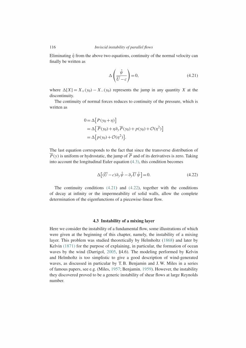
116 Inviscid instability of parallel flows

Eliminating η from the above two equations, continuity of the normal velocity canfinally be written as

(ψ

U −c

)=0, (4.21)

where [X ] = X+(y0)− X−(y0) represents the jump in any quantity X at thediscontinuity.

The continuity of normal forces reduces to continuity of the pressure, which iswritten as

0=[P(y0 +η)

]=[

P(y0)+η∂y P(y0)+ p(y0)+O(η2)]

=[

p(y0)+O(η2)].

The last equation corresponds to the fact that since the transverse distribution ofP(y) is uniform or hydrostatic, the jump of P and of its derivatives is zero. Takinginto account the longitudinal Euler equation (4.3), this condition becomes

[(U −c)∂yψ −∂yU ψ

]=0. (4.22)

The continuity conditions (4.21) and (4.22), together with the conditionsof decay at infinity or the impermeability of solid walls, allow the completedetermination of the eigenfunctions of a piecewise-linear flow.

4.3 Instability of a mixing layer

Here we consider the instability of a fundamental flow, some illustrations of whichwere given at the beginning of this chapter, namely, the instability of a mixinglayer. This problem was studied theoretically by Helmholtz (1868) and later byKelvin (1871) for the purpose of explaining, in particular, the formation of oceanwaves by the wind (Darrigol, 2005, §4.6). The modeling performed by Kelvinand Helmholtz is too simplistic to give a good description of wind-generatedwaves, as discussed in particular by T. B. Benjamin and J. W. Miles in a seriesof famous papers, see e.g. (Miles, 1957; Benjamin, 1959). However, the instabilitythey discovered proved to be a generic instability of shear flows at large Reynoldsnumber.

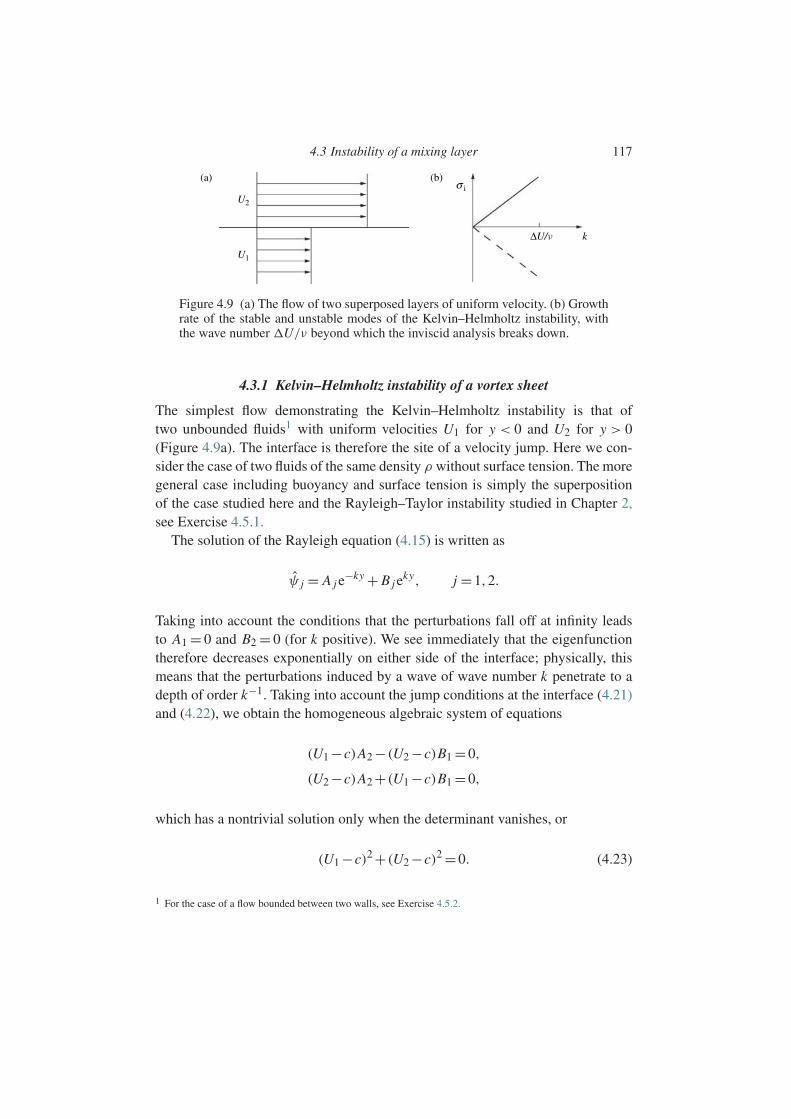
4.3 Instability of a mixing layer 117

U2

(a) (b)σ i

U1

∆U/ν k

Figure 4.9 (a) The flow of two superposed layers of uniform velocity. (b) Growthrate of the stable and unstable modes of the Kelvin–Helmholtz instability, withthe wave number U/ν beyond which the inviscid analysis breaks down.

4.3.1 Kelvin–Helmholtz instability of a vortex sheet

The simplest flow demonstrating the Kelvin–Helmholtz instability is that oftwo unbounded fluids1 with uniform velocities U1 for y < 0 and U2 for y > 0(Figure 4.9a). The interface is therefore the site of a velocity jump. Here we con-sider the case of two fluids of the same density ρ without surface tension. The moregeneral case including buoyancy and surface tension is simply the superpositionof the case studied here and the Rayleigh–Taylor instability studied in Chapter 2,see Exercise 4.5.1.

The solution of the Rayleigh equation (4.15) is written as

ψ j = A j e−ky + B j e

ky, j =1,2.

Taking into account the conditions that the perturbations fall off at infinity leadsto A1 = 0 and B2 = 0 (for k positive). We see immediately that the eigenfunctiontherefore decreases exponentially on either side of the interface; physically, thismeans that the perturbations induced by a wave of wave number k penetrate to adepth of order k−1. Taking into account the jump conditions at the interface (4.21)and (4.22), we obtain the homogeneous algebraic system of equations

(U1 −c)A2 −(U2 −c)B1 =0,

(U2 −c)A2 +(U1 −c)B1 =0,

which has a nontrivial solution only when the determinant vanishes, or

(U1 −c)2 +(U2 −c)2 =0. (4.23)

1 For the case of a flow bounded between two walls, see Exercise 4.5.2.

118 Inviscid instability of parallel flows

This is the desired dispersion relation, which shows that there exist two modescorresponding to two complex-conjugate eigenvalues

c = ω

k=Uav ± iU, (4.24)

where we have introduced the average speed Uav = (U1 + U2)/2 and the half-difference of the speeds U = (U1 −U2)/2. From the viewpoint of the temporalstability of a perturbation of real wave number, the speed cr and the temporalgrowth rate ωi = kci of these modes are

cr =Uav, ωi =±k U. (4.25)

Therefore, both modes propagate at the same speed equal to the average speed Uav

(waves are not dispersive), and because of the mode with positive growth rate theflow is unstable for any velocity difference, no matter how small. Moreover, it isunstable to any perturbation, no matter what its wave number k, with growth rateincreasing linearly with k (Figure 4.9b).

The unphysical conclusion that the growth rate is unbounded at large wave num-bers (small wavelengths) is a consequence of the fact that all effects of viscousdiffusion have been ignored. In fact, inertial effects dominate viscous effects forwave numbers such that ρkU 2 µk2U , i.e., k U/ν, but they cannot beignored for k U/ν. The quantity U/ν therefore determines the wave numberscale beyond which the above analysis is no longer valid (Figure 4.9b). A morerealistic model that avoids the divergence of the growth rate at large wave numberswhile retaining the inviscid approximation will be discussed later on.

The Kelvin–Helmholtz instability mechanism can be explained as a sort of“Bernoulli effect.” Let us consider the flow in a reference frame moving at theaverage speed (Figure 4.10), in which the speeds of the fluids are U1 =−U andU2 =U and the speed of the perturbations vanishes according to (4.25). Above aperturbation η> 0 of the shear layer the fluid is accelerated owing to the fact thatthe cross-sectional area perpendicular to the flow is decreased. This perturbationplays a role to a depth of order k−1, the only length scale in the problem, on eitherside of the interface. The order of magnitude of the velocity perturbation is there-fore such that ηU ∼u/k owing to the incompressibility of the fluid. This velocityexcess above a crest leads to a pressure decrease of order p ∼ −ρUu accord-ing to the linearized Bernoulli theorem, so that the pressure difference acrossthe interface amplifies the perturbation. We then obtain the growth rate from aone-dimensional momentum balance as

σ = 1

u

du

dt=− 1

ρu

∂p

∂x∼− kp

ρu∼ kU.

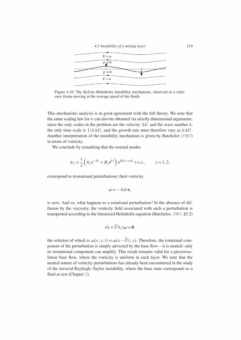
4.3 Instability of a mixing layer 119

Figure 4.10 The Kelvin–Helmholtz instability mechanism, observed in a refer-ence frame moving at the average speed of the fluids.

This mechanistic analysis is in good agreement with the full theory. We note thatthe same scaling law for σ can also be obtained via strictly dimensional arguments:since the only scales in the problem are the velocity U and the wave number k,the only time scale is 1/kU , and the growth rate must therefore vary as kU .Another interpretation of the instability mechanism is given by Batchelor (1967)in terms of vorticity.

We conclude by remarking that the normal modes

ψ j = 1

2

(A j e

−ky + B j eky)

ei(kx−ωt)+c.c., j =1,2,

correspond to irrotational perturbations; their vorticity

ω=−ψ ez

is zero. And so, what happens to a rotational perturbation? In the absence of dif-fusion by the viscosity, the vorticity field associated with such a perturbation istransported according to the linearized Helmholtz equation (Batchelor, 1967, §5.2)

(∂t +U∂x )ω=0,

the solution of which is ω(x, y, t)=ω(x −Ut, y). Therefore, the rotational com-ponent of the perturbation is simply advected by the base flow – it is neutral: onlyits irrotational component can amplify. This result remains valid for a piecewise-linear base flow, where the vorticity is uniform in each layer. We note that theneutral nature of vorticity perturbations has already been encountered in the studyof the inviscid Rayleigh–Taylor instability, where the base state corresponds to afluid at rest (Chapter 2).

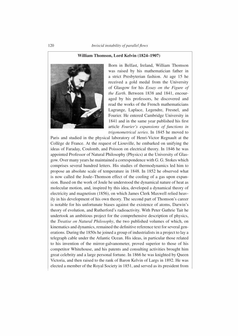
120 Inviscid instability of parallel flows

William Thomson, Lord Kelvin (1824–1907)

Born in Belfast, Ireland, William Thomsonwas raised by his mathematician father ina strict Presbyterian fashion. At age 15 hereceived a gold medal from the Universityof Glasgow for his Essay on the Figure ofthe Earth. Between 1838 and 1841, encour-aged by his professors, he discovered andread the works of the French mathematiciansLagrange, Laplace, Legendre, Fresnel, andFourier. He entered Cambridge University in1841 and in the same year published his firstarticle Fourier’s expansions of functions intrigonometrical series. In 1845 he moved to

Paris and studied in the physical laboratory of Henri-Victor Regnault at theCollege de France. At the request of Liouville, he embarked on unifying theideas of Faraday, Coulomb, and Poisson on electrical theory. In 1846 he wasappointed Professor of Natural Philosophy (Physics) at the University of Glas-gow. Over many years he maintained a correspondence with G. G. Stokes whichcomprises several hundred letters. His studies of thermodynamics led him topropose an absolute scale of temperature in 1848. In 1852 he observed whatis now called the Joule–Thomson effect of the cooling of a gas upon expan-sion. Based on the work of Joule he understood the dynamical nature of heat asmolecular motion, and, inspired by this idea, developed a dynamical theory ofelectricity and magnetism (1856), on which James Clerk Maxwell relied heav-ily in his development of his own theory. The second part of Thomson’s careeris notable for his unfortunate biases against the existence of atoms, Darwin’stheory of evolution, and Rutherford’s radioactivity. With Peter Guthrie Tait heundertook an ambitious project for the comprehensive description of physics,the Treatise on Natural Philosophy, the two published volumes of which, onkinematics and dynamics, remained the definitive reference text for several gen-erations. During the 1850s he joined a group of industrialists in a project to lay atelegraph cable under the Atlantic Ocean. His ideas, in particular those relatedto his invention of the mirror-galvanometer, proved superior to those of hiscompetitor Whitehouse, and his patents and consulting activities brought himgreat celebrity and a large personal fortune. In 1866 he was knighted by QueenVictoria, and then raised to the rank of Baron Kelvin of Largs in 1892. He waselected a member of the Royal Society in 1851, and served as its president from

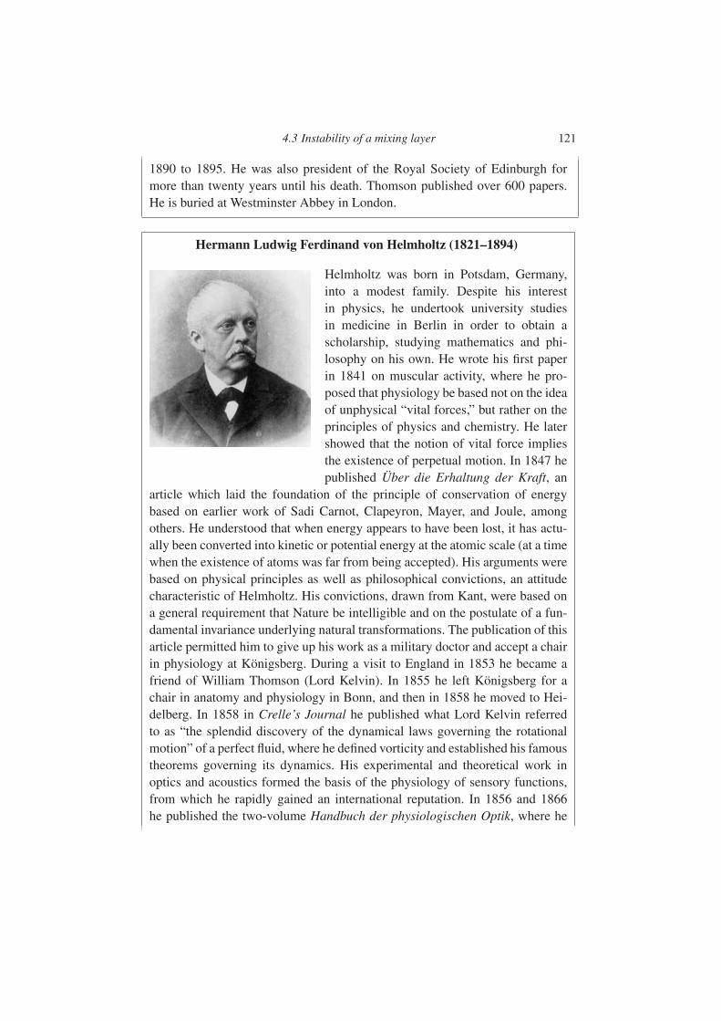
4.3 Instability of a mixing layer 121

1890 to 1895. He was also president of the Royal Society of Edinburgh formore than twenty years until his death. Thomson published over 600 papers.He is buried at Westminster Abbey in London.

Hermann Ludwig Ferdinand von Helmholtz (1821–1894)

Helmholtz was born in Potsdam, Germany,into a modest family. Despite his interestin physics, he undertook university studiesin medicine in Berlin in order to obtain ascholarship, studying mathematics and phi-losophy on his own. He wrote his first paperin 1841 on muscular activity, where he pro-posed that physiology be based not on the ideaof unphysical “vital forces,” but rather on theprinciples of physics and chemistry. He latershowed that the notion of vital force impliesthe existence of perpetual motion. In 1847 hepublished Uber die Erhaltung der Kraft, an

article which laid the foundation of the principle of conservation of energybased on earlier work of Sadi Carnot, Clapeyron, Mayer, and Joule, amongothers. He understood that when energy appears to have been lost, it has actu-ally been converted into kinetic or potential energy at the atomic scale (at a timewhen the existence of atoms was far from being accepted). His arguments werebased on physical principles as well as philosophical convictions, an attitudecharacteristic of Helmholtz. His convictions, drawn from Kant, were based ona general requirement that Nature be intelligible and on the postulate of a fun-damental invariance underlying natural transformations. The publication of thisarticle permitted him to give up his work as a military doctor and accept a chairin physiology at Konigsberg. During a visit to England in 1853 he became afriend of William Thomson (Lord Kelvin). In 1855 he left Konigsberg for achair in anatomy and physiology in Bonn, and then in 1858 he moved to Hei-delberg. In 1858 in Crelle’s Journal he published what Lord Kelvin referredto as “the splendid discovery of the dynamical laws governing the rotationalmotion” of a perfect fluid, where he defined vorticity and established his famoustheorems governing its dynamics. His experimental and theoretical work inoptics and acoustics formed the basis of the physiology of sensory functions,from which he rapidly gained an international reputation. In 1856 and 1866he published the two-volume Handbuch der physiologischen Optik, where he

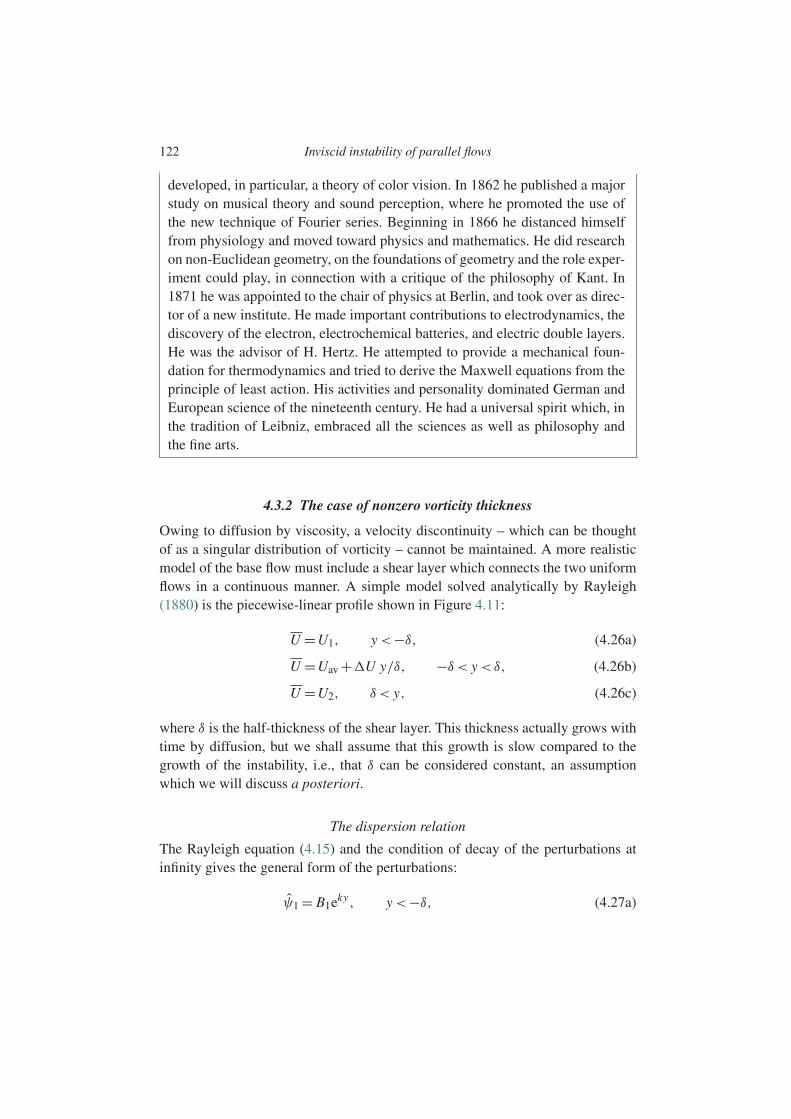
122 Inviscid instability of parallel flows

developed, in particular, a theory of color vision. In 1862 he published a majorstudy on musical theory and sound perception, where he promoted the use ofthe new technique of Fourier series. Beginning in 1866 he distanced himselffrom physiology and moved toward physics and mathematics. He did researchon non-Euclidean geometry, on the foundations of geometry and the role exper-iment could play, in connection with a critique of the philosophy of Kant. In1871 he was appointed to the chair of physics at Berlin, and took over as direc-tor of a new institute. He made important contributions to electrodynamics, thediscovery of the electron, electrochemical batteries, and electric double layers.He was the advisor of H. Hertz. He attempted to provide a mechanical foun-dation for thermodynamics and tried to derive the Maxwell equations from theprinciple of least action. His activities and personality dominated German andEuropean science of the nineteenth century. He had a universal spirit which, inthe tradition of Leibniz, embraced all the sciences as well as philosophy andthe fine arts.

4.3.2 The case of nonzero vorticity thickness

Owing to diffusion by viscosity, a velocity discontinuity – which can be thoughtof as a singular distribution of vorticity – cannot be maintained. A more realisticmodel of the base flow must include a shear layer which connects the two uniformflows in a continuous manner. A simple model solved analytically by Rayleigh(1880) is the piecewise-linear profile shown in Figure 4.11:

U =U1, y <−δ, (4.26a)

U =Uav +U y/δ, −δ < y <δ, (4.26b)

U =U2, δ < y, (4.26c)

where δ is the half-thickness of the shear layer. This thickness actually grows withtime by diffusion, but we shall assume that this growth is slow compared to thegrowth of the instability, i.e., that δ can be considered constant, an assumptionwhich we will discuss a posteriori.

The dispersion relation

The Rayleigh equation (4.15) and the condition of decay of the perturbations atinfinity gives the general form of the perturbations:

ψ1 = B1eky, y <−δ, (4.27a)

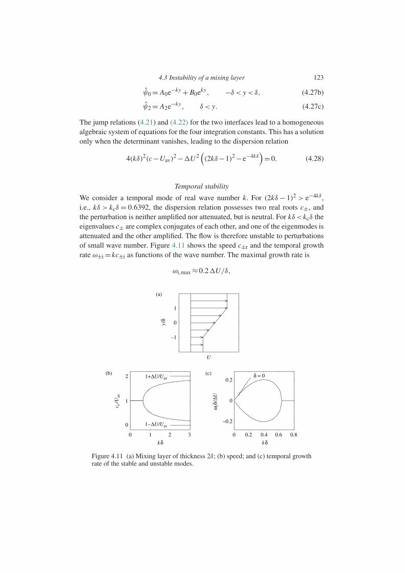
4.3 Instability of a mixing layer 123

ψ0 = A0e−ky + B0eky, −δ < y <δ, (4.27b)

ψ2 = A2e−ky, δ < y. (4.27c)

The jump relations (4.21) and (4.22) for the two interfaces lead to a homogeneousalgebraic system of equations for the four integration constants. This has a solutiononly when the determinant vanishes, leading to the dispersion relation

4(kδ)2(c−Uav)2 −U 2

((2kδ−1)2 −e−4kδ

)=0. (4.28)

Temporal stability

We consider a temporal mode of real wave number k. For (2kδ − 1)2 > e−4kδ,i.e., kδ > kcδ = 0.6392, the dispersion relation possesses two real roots c±, andthe perturbation is neither amplified nor attenuated, but is neutral. For kδ<kcδ theeigenvalues c± are complex conjugates of each other, and one of the eigenmodes isattenuated and the other amplified. The flow is therefore unstable to perturbationsof small wave number. Figure 4.11 shows the speed c±r and the temporal growthrate ω±i = kc±i as functions of the wave number. The maximal growth rate is

ωi,max ≈0.2U/δ,

(a)

(b) (c)

1

20.2

ωiδ

/∆U

0

–0.2

1+∆U/Uav

1–∆U/Uav

1

0

c r/U

av

0 1 2 3 0 0.2 0.4 0.6 0.8

0

–1

U

y/δ

δ = 0

kδ kδ

Figure 4.11 (a) Mixing layer of thickness 2δ; (b) speed; and (c) temporal growthrate of the stable and unstable modes.

124 Inviscid instability of parallel flows

and corresponds to kmaxδ≈0.4. For kδ1, i.e., perturbations of wavelength largecompared to the vorticity thickness, we recover the dimensional growth rate ω±i =±kU for a vorticity sheet of zero thickness, as we would expect.

A better model of the base flow which is more regular than the piecewise-linearflow is that described by the hyperbolic tangent function:

U =Uav +U tanh(y/δ). (4.29)

Numerical solution of the Rayleigh equation leads to a stability curve very close tothat of Figure 4.11 (Michalke, 1964). The cutoff wave number is koffδ=1, and themaximum temporal growth rate ωi,maxδ/U∞ ≈ 0.2 occurs at kmaxδ ≈ 0.44, valueswhich are very close to those of the piecewise-linear flow.

Finally, the Kelvin–Helmholtz instability is manifested in the growth of pertur-bations with wavelength large compared to the thickness δ over an advective timeof order δ/U . This result is obtained more generally for any shear flow at largeReynolds number when the velocity profile has an inflection point, including jetsand wakes.

Spatial stability and the convective–absolute transition

Since a study of spatial stability is meaningful only if the instability is convec-tive and not absolute, the first step is to determine the condition for convectiveinstability as discussed in the preceding chapter. The convective–absolute transi-tion corresponds to the vanishing of the group velocity for a wave number k0 to bedetermined. Differentiating the dispersion relation and setting ∂ω/∂k =0, we find

ω0δ

Uav= k0δ− 1

2

(U

Uav

)2

(2k0δ−1+e−4k0δ). (4.30)

Substituting this expression into the dispersion relation (4.28), we see that k0 is thesolution of the equation

(2k0δ−1+e−4k0δ)2(U

Uav

)2

−[(2k0δ−1)2 −e−4k0δ]=0. (4.31)

Numerical solution of this equation allows the determination of the complex wavenumber k0U/Uav at which the group velocity vanishes, and then the corre-sponding complex frequency ω0U/Uav can be obtained. It turns out that theabsolute growth rate ω0i is negative for |U/Uav|< 1 and becomes positive for|U/Uav|>1 (Huerre and Rossi, 1998). For |U/Uav|<1, that is, when the twofluids flow together, the instability is convective, and the mixing layer behaves asa noise amplifier. For |U/Uav|> 1, when the two fluids flow in opposite direc-tions, the instability is absolute and the mixing layer behaves like an oscillator

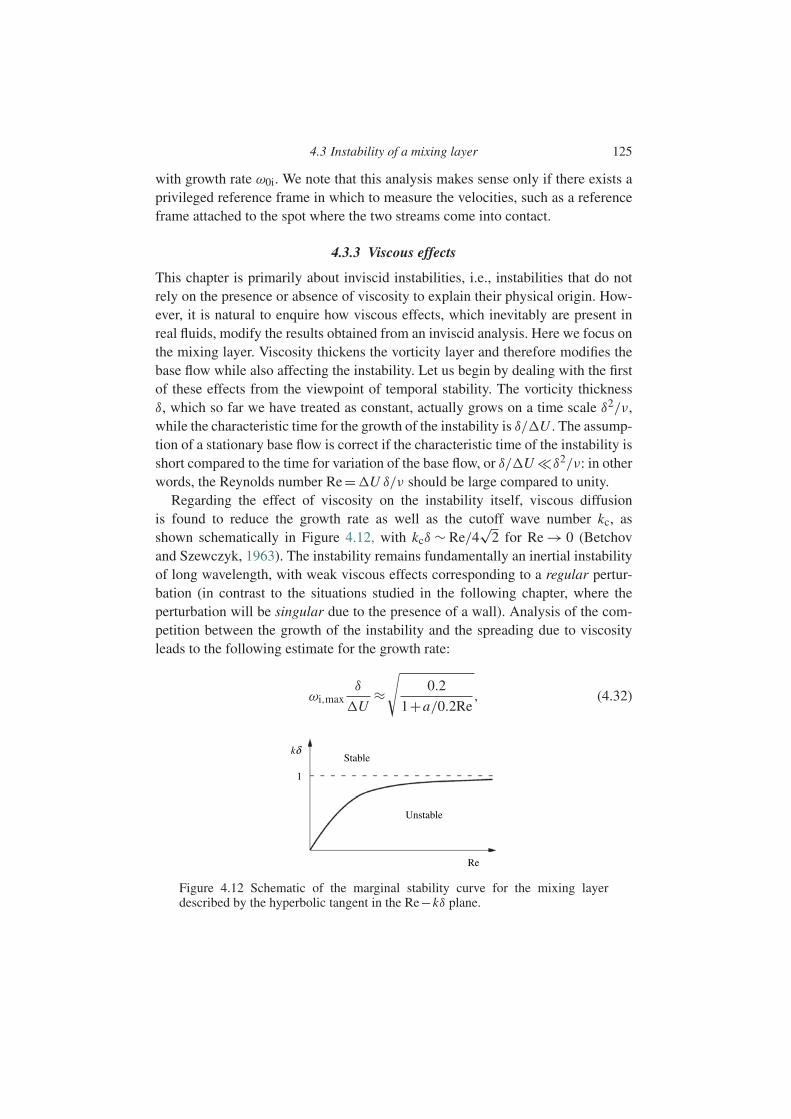
4.3 Instability of a mixing layer 125

with growth rate ω0i. We note that this analysis makes sense only if there exists aprivileged reference frame in which to measure the velocities, such as a referenceframe attached to the spot where the two streams come into contact.

4.3.3 Viscous effects

This chapter is primarily about inviscid instabilities, i.e., instabilities that do notrely on the presence or absence of viscosity to explain their physical origin. How-ever, it is natural to enquire how viscous effects, which inevitably are present inreal fluids, modify the results obtained from an inviscid analysis. Here we focus onthe mixing layer. Viscosity thickens the vorticity layer and therefore modifies thebase flow while also affecting the instability. Let us begin by dealing with the firstof these effects from the viewpoint of temporal stability. The vorticity thicknessδ, which so far we have treated as constant, actually grows on a time scale δ2/ν,while the characteristic time for the growth of the instability is δ/U . The assump-tion of a stationary base flow is correct if the characteristic time of the instability isshort compared to the time for variation of the base flow, or δ/U δ2/ν: in otherwords, the Reynolds number Re=U δ/ν should be large compared to unity.

Regarding the effect of viscosity on the instability itself, viscous diffusionis found to reduce the growth rate as well as the cutoff wave number kc, asshown schematically in Figure 4.12, with kcδ ∼ Re/4

√2 for Re → 0 (Betchov

and Szewczyk, 1963). The instability remains fundamentally an inertial instabilityof long wavelength, with weak viscous effects corresponding to a regular pertur-bation (in contrast to the situations studied in the following chapter, where theperturbation will be singular due to the presence of a wall). Analysis of the com-petition between the growth of the instability and the spreading due to viscosityleads to the following estimate for the growth rate:

ωi,maxδ

U≈√

0.2

1+a/0.2Re, (4.32)

Stable

Unstable

Re

1

kδ

Figure 4.12 Schematic of the marginal stability curve for the mixing layerdescribed by the hyperbolic tangent in the Re−kδ plane.

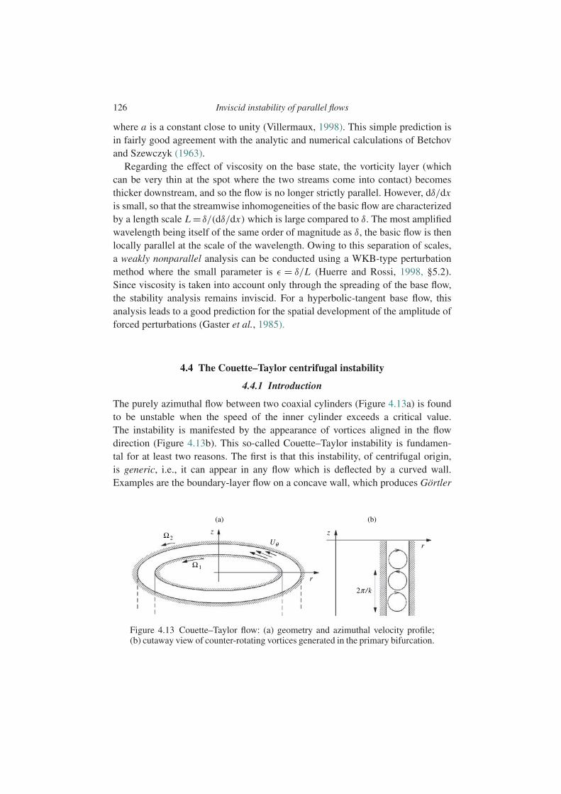
126 Inviscid instability of parallel flows

where a is a constant close to unity (Villermaux, 1998). This simple prediction isin fairly good agreement with the analytic and numerical calculations of Betchovand Szewczyk (1963).

Regarding the effect of viscosity on the base state, the vorticity layer (whichcan be very thin at the spot where the two streams come into contact) becomesthicker downstream, and so the flow is no longer strictly parallel. However, dδ/dxis small, so that the streamwise inhomogeneities of the basic flow are characterizedby a length scale L = δ/(dδ/dx) which is large compared to δ. The most amplifiedwavelength being itself of the same order of magnitude as δ, the basic flow is thenlocally parallel at the scale of the wavelength. Owing to this separation of scales,a weakly nonparallel analysis can be conducted using a WKB-type perturbationmethod where the small parameter is ε = δ/L (Huerre and Rossi, 1998, §5.2).Since viscosity is taken into account only through the spreading of the base flow,the stability analysis remains inviscid. For a hyperbolic-tangent base flow, thisanalysis leads to a good prediction for the spatial development of the amplitude offorced perturbations (Gaster et al., 1985).

4.4 The Couette–Taylor centrifugal instability

4.4.1 Introduction

The purely azimuthal flow between two coaxial cylinders (Figure 4.13a) is foundto be unstable when the speed of the inner cylinder exceeds a critical value.The instability is manifested by the appearance of vortices aligned in the flowdirection (Figure 4.13b). This so-called Couette–Taylor instability is fundamen-tal for at least two reasons. The first is that this instability, of centrifugal origin,is generic, i.e., it can appear in any flow which is deflected by a curved wall.Examples are the boundary-layer flow on a concave wall, which produces Gortler

(a) (b)

z z

r

r

2π /k

Uθ

Ω1

Ω2

Figure 4.13 Couette–Taylor flow: (a) geometry and azimuthal velocity profile;(b) cutaway view of counter-rotating vortices generated in the primary bifurcation.

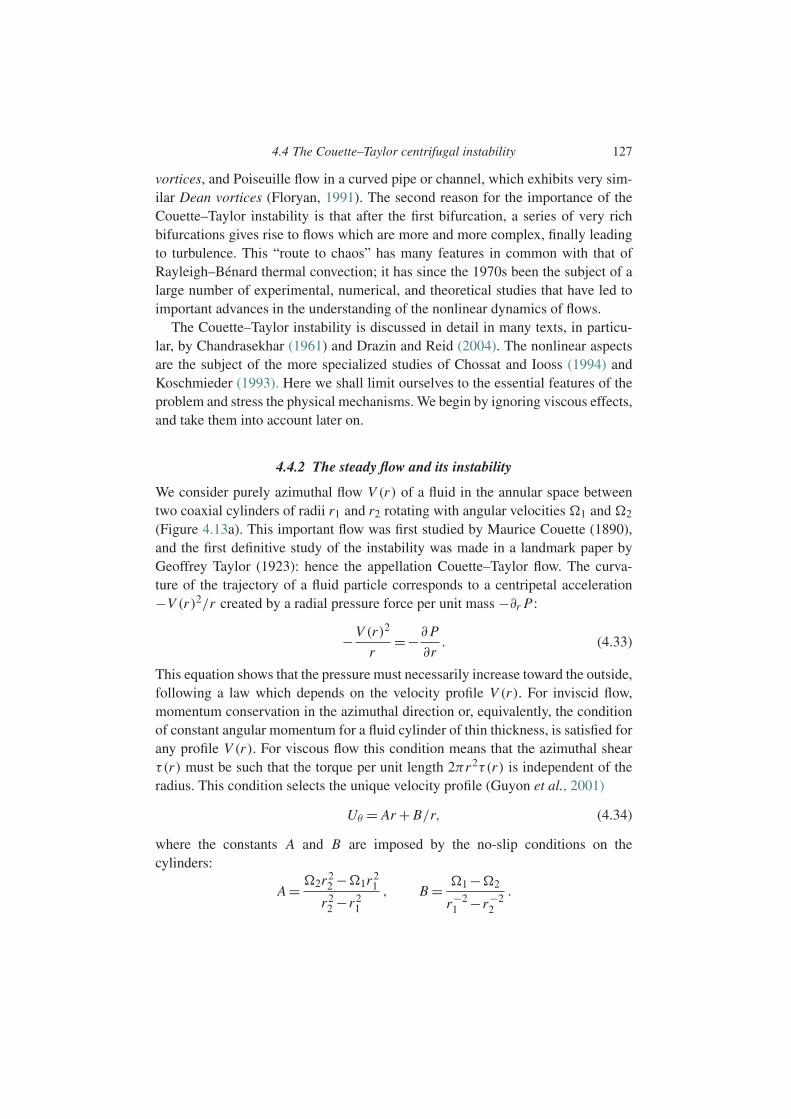
4.4 The Couette–Taylor centrifugal instability 127

vortices, and Poiseuille flow in a curved pipe or channel, which exhibits very sim-ilar Dean vortices (Floryan, 1991). The second reason for the importance of theCouette–Taylor instability is that after the first bifurcation, a series of very richbifurcations gives rise to flows which are more and more complex, finally leadingto turbulence. This “route to chaos” has many features in common with that ofRayleigh–Benard thermal convection; it has since the 1970s been the subject of alarge number of experimental, numerical, and theoretical studies that have led toimportant advances in the understanding of the nonlinear dynamics of flows.

The Couette–Taylor instability is discussed in detail in many texts, in particu-lar, by Chandrasekhar (1961) and Drazin and Reid (2004). The nonlinear aspectsare the subject of the more specialized studies of Chossat and Iooss (1994) andKoschmieder (1993). Here we shall limit ourselves to the essential features of theproblem and stress the physical mechanisms. We begin by ignoring viscous effects,and take them into account later on.

4.4.2 The steady flow and its instability

We consider purely azimuthal flow V (r) of a fluid in the annular space betweentwo coaxial cylinders of radii r1 and r2 rotating with angular velocities 1 and 2

(Figure 4.13a). This important flow was first studied by Maurice Couette (1890),and the first definitive study of the instability was made in a landmark paper byGeoffrey Taylor (1923): hence the appellation Couette–Taylor flow. The curva-ture of the trajectory of a fluid particle corresponds to a centripetal acceleration−V (r)2/r created by a radial pressure force per unit mass −∂r P:

−V (r)2

r=−∂P

∂r. (4.33)

This equation shows that the pressure must necessarily increase toward the outside,following a law which depends on the velocity profile V (r). For inviscid flow,momentum conservation in the azimuthal direction or, equivalently, the conditionof constant angular momentum for a fluid cylinder of thin thickness, is satisfied forany profile V (r). For viscous flow this condition means that the azimuthal shearτ(r) must be such that the torque per unit length 2πr2τ(r) is independent of theradius. This condition selects the unique velocity profile (Guyon et al., 2001)

Uθ = Ar + B/r, (4.34)

where the constants A and B are imposed by the no-slip conditions on thecylinders:

A = 2r22 −1r2

1

r22 −r2

1

, B = 1 −2

r−21 −r−2

2

.

128 Inviscid instability of parallel flows

The first experiments on this type of flow were performed by MauriceCouette (1890) with the goal of determining the fluid viscosity. His apparatusallowed only the outer cylinder to rotate, and the torque was measured on theinner cylinder. These experiments showed that over a large range of velocity 2

the torque varies linearly with this velocity, consistent with the velocity profile(4.34). These experiments also showed that beyond a certain velocity 2 whichis difficult to define precisely, the torque increases strongly, an observation thatCouette correctly attributed to an instability of the flow (4.34) and the appearanceof turbulent motion.

These experiments were repeated by Geoffrey I. Taylor (1923) using an appa-ratus which permitted the inner cylinder to also be turned. The large axial lengthof the cylinders, 90 cm or one hundred times the annular spacing r2 −r1, made itpossible to largely avoid end effects at the top and bottom boundaries. The mainobservation of Taylor was that if only the inner cylinder is turned, an instability ismanifested beyond a certain velocity 1 as the appearance of a new flow which isnot turbulent but instead stationary with a particular spatial structure; this structurecorresponds to pairs of counter-rotating toroidal vortices that are periodic in theaxial direction with wave number k such that 2π/k ≈ 2(r2 − r1) (Figures 4.13band 4.14a). This instability is also observed for nonzero 2: Figure 4.15 shows theinstability threshold in the plane of Reynolds numbers formed using the cylindervelocities and spacing:

Re1 = 1r1(r2 −r1)

ν, Re2 = 2r2(r2 −r1)

ν. (4.35)

(a) (b)

Figure 4.14 The annular vortices of Taylor. (a) Ta/Tac = 1.1; (b) Ta/Tac = 6.0,and the vortices now display waves after a second instability has appeared (λ=2π R/4) (Fenstermacher et al., 1979).

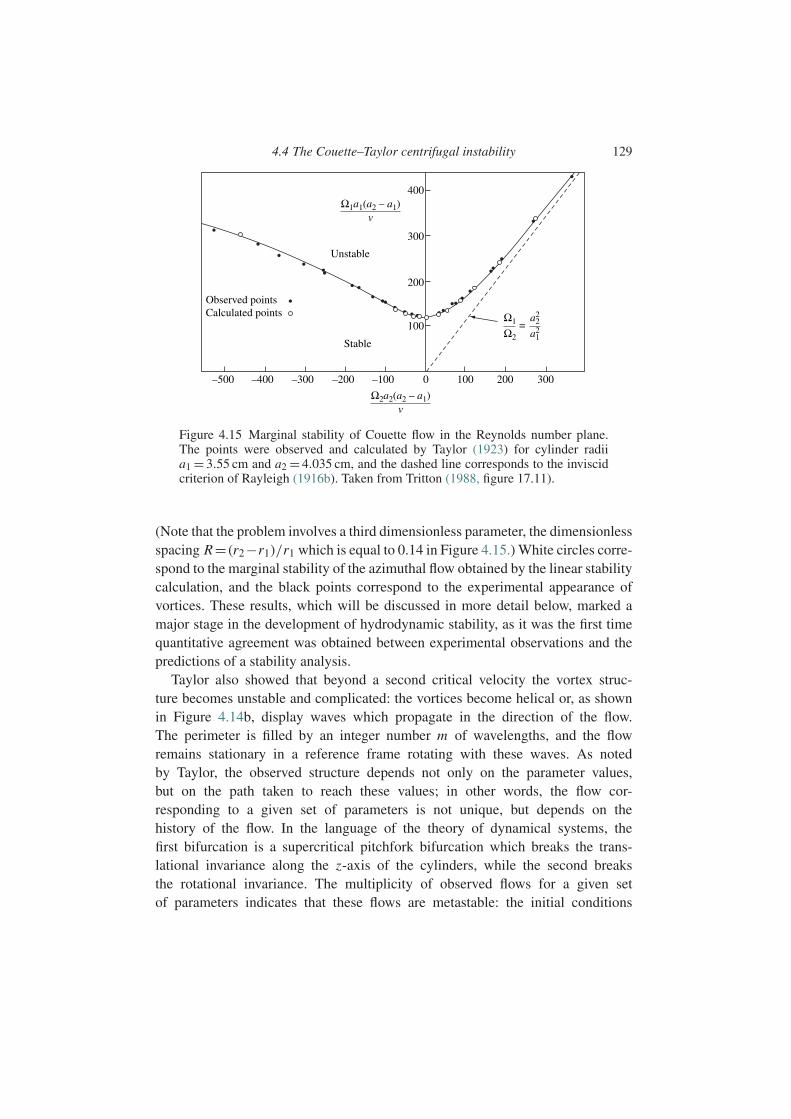
4.4 The Couette–Taylor centrifugal instability 129

–500 –400 –300 –200 –100

100

200

300

400

Unstable

Stable

Observed pointsCalculated points

0 100

Ω2a2(a2 – a1)v

Ω1

Ω2

a22

a21

200 300

=

Ω1a1(a2 – a1)v

Figure 4.15 Marginal stability of Couette flow in the Reynolds number plane.The points were observed and calculated by Taylor (1923) for cylinder radiia1 = 3.55 cm and a2 = 4.035 cm, and the dashed line corresponds to the inviscidcriterion of Rayleigh (1916b). Taken from Tritton (1988, figure 17.11).

(Note that the problem involves a third dimensionless parameter, the dimensionlessspacing R=(r2−r1)/r1 which is equal to 0.14 in Figure 4.15.) White circles corre-spond to the marginal stability of the azimuthal flow obtained by the linear stabilitycalculation, and the black points correspond to the experimental appearance ofvortices. These results, which will be discussed in more detail below, marked amajor stage in the development of hydrodynamic stability, as it was the first timequantitative agreement was obtained between experimental observations and thepredictions of a stability analysis.

Taylor also showed that beyond a second critical velocity the vortex struc-ture becomes unstable and complicated: the vortices become helical or, as shownin Figure 4.14b, display waves which propagate in the direction of the flow.The perimeter is filled by an integer number m of wavelengths, and the flowremains stationary in a reference frame rotating with these waves. As notedby Taylor, the observed structure depends not only on the parameter values,but on the path taken to reach these values; in other words, the flow cor-responding to a given set of parameters is not unique, but depends on thehistory of the flow. In the language of the theory of dynamical systems, thefirst bifurcation is a supercritical pitchfork bifurcation which breaks the trans-lational invariance along the z-axis of the cylinders, while the second breaksthe rotational invariance. The multiplicity of observed flows for a given setof parameters indicates that these flows are metastable: the initial conditions

130 Inviscid instability of parallel flows

leading to each of these attractors correspond to a basin of attraction of finiteextent.

The situation regarding the stability of inviscid flow can be phrased in verysimple terms: if the pressure distribution P(r) is such that a fluid particle perturbedfrom its circular equilibrium trajectory is subject to a restoring force, the azimuthalflow is stable, otherwise, it is unstable. For viscous flow this instability conditionis necessary but not sufficient: the instability requires that the destabilizing forcebe larger than the viscous retarding force. We shall make these instability criteriamore precise below.

4.4.3 The instability criterion for inviscid flow

Since the instability of Couette flow results from an inertial mechanism, aninstability criterion and insight into the mechanism can be obtained by initiallyneglecting viscous effects. Following von Karman (1934), we consider a fluidring of radius r and velocity V for which the angular momentum per unit massis J = r V and the circulation2 is 2π J . From (4.33) the centripetal pressure gradi-ent exerted on this ring is then V 2/r = J 2/r3. According to the Kelvin theorem, adeformation of this ring into a ring of radius r +dr must conserve the circulation2π J (Batchelor, 1967, §5.3), i.e., it must conserve its angular momentum J . Thepressure gradient necessary to just keep the ring in its new position is thereforeJ (r)2/(r + dr)3. If the existing pressure gradient J (r + dr)2/(r + dr)3 is largerthan J (r)2/(r +dr)3, the ring is subject to a force tending to restore it to its initialposition; otherwise, this gradient tends to amplify the deformation. We then deducethat a necessary and sufficient condition for instability to axisymmetric perturba-tions is J (r + dr)2 < J (r)2. This instability condition is therefore the conditionthat the squared angular momentum decrease:

dJ 2

dr<0, where J = r V . (4.36)

In other words, the flow is unstable if the increase of the pressure with radius is tooslow, with the result that r3∂r P(r) decreases with increasing r . The criterion (4.36)was originally obtained by Rayleigh (1916b), using a clever argument involvingthe analogy with the instability of a fluid at rest under gravity with an unstabledensity stratification. This criterion was confirmed by a complete linear stability

2 The circulation of the velocity field u(x) round a closed curve C is defined as (Batchelor, 1967, §2.6)∫C

u ·dx.

4.4 The Couette–Taylor centrifugal instability 131

calculation for non-axisymmetric perturbations proportional to ei(kz+mθ−ωt): non-axisymmetric perturbations (m =0) are found to be more stable than axisymmetricones (m = 0), the latter being unstable if and only if the Rayleigh criterion is sat-isfied. The determination of the criterion for axisymmetric perturbations is left asan exercise (Exercise 4.5.4).

For Couette flow (4.34), the Rayleigh stability criterion (4.36) becomes

d

dr(Ar2 + B)2 =4Ar2 Uθ <0,

i.e., A<0, or2r2

2 <1r21 . (4.37)

Inviscid Couette flow is therefore stable to axisymmetric perturbations if the cir-culation of the outer cylinder 2π2r2

2 is smaller than that of the inner cylinder2π1r2

1 .As already mentioned, Rayleigh (1916b) pointed out that the centrifugal insta-

bility described above is very similar to the instability of a density-stratified fluid inthe gravity field (Rayleigh–Taylor instability): the radial pressure gradient (4.33)here plays a role analogous to the buoyancy force. More precisely, the instabilitycondition (4.36) that the angular momentum decrease toward the outside is anal-ogous to the condition that the density increase toward the top. Putting it anotherway, the unstable stratification of centrifugal force is analogous to the unstablestratification of density.

4.4.4 The effect of viscosity: the Taylor number

According to the Rayleigh criterion, even the slightest rotation 1 of the innercylinder when the outer cylinder is fixed (2 = 0) allows the possibility of aninstability. In reality, the appearance of the instability is postponed by viscous dif-fusion, and it occurs only beyond a nonzero 1. Figure 4.15 shows the marginalstability curve obtained by Taylor (1923) in the plane of the rotation velocities 1

and 2 normalized by ν/r1(r2 − r1). This curve is an interpolation between theexperimental points and the points obtained from the detailed stability calculationdescribed below. We see that the agreement between experiment and calculationis excellent, and that the Rayleigh criterion, which ignores the stabilizing effect ofthe viscosity, gives the correct asymptotic behavior for large velocities of the samesign, the conditions under which viscous effects are effectively small compared toinertial ones.

We now show how the Taylor number controlling the instability arises, howthis problem is related to the Rayleigh–Benard problem, and how the Taylor num-ber is related to the Rayleigh number. We consider an axisymmetric perturbation

132 Inviscid instability of parallel flows

(corresponding to the observed vortices). For such a perturbation we can write thelinearized equations for the perturbations of the radial and azimuthal velocities ur

and uθ as (Drazin and Reid, 2004, §17; Chandrasekhar, 1961, chapter 7)

∂ur

∂t=− 1

ρ

∂p

∂r+ν∗ur + 2U θuθ

r, (4.38a)

∂uθ

∂t= ν∗uθ −(D∗U θ )ur , (4.38b)

where the starred operators are defined as

D∗ = ∂

∂r+ 1

r, ∗ = ∂2

∂r2+ 1

r

∂

∂r− 1

r2+ ∂2

∂z2.

In each of these equations the first terms on the right-hand side correspond toviscous retardation, and the last term is an inertial term. In the first equation theinertial term arises from the rotation of the vector eθ in the frame of a fluid particle,and in the second the inertial term is the sum of the advection by ur of the radialgradient ∂rU θ of the base flow and the term urU θ /r from the rotation of the vectorer . The complete analysis of this set of linearized equations is outside the scopeof this text. However, insight into the physical mechanism of the instability isgained by discussing the analogy between this problem and the Rayleigh–Benardproblem.3

These two equations are quite similar to the equations (2.49) of the Rayleigh–Benard problem (Chapter 2). The radial speed ur generated by the radial inertialforce corresponds to the vertical speed v due to the buoyancy force, and theazimuthal speed uθ corresponds to the temperature difference δT . To make theanalogy between the two problems clearer, we artificially distinguish a radial vis-cosity νr and an azimuthal viscosity νθ , and analyze the case νr/νθ 1 in the sameway as for the Rayleigh–Benard problem at large Prandtl number Pr = ν/κ . For afluid particle displaced from its equilibrium position, the radial motion relaxesmuch more quickly to equilibrium than the azimuthal motion. In addition, like

3 The acceleration is the Lagrangian derivative of the velocity:

a= d

dt(Ur er +Uθ eθ )=

dUr

dter +Ur

der

dt+ dUθ

dteθ +Uθ

deθdt

.

Decomposing the velocity into the sum of a base flow U θ eθ and perturbations ur er +uθ eθ , we obtain

ar = dur

dt− (U θ +uθ )

2

r,

aθ = duθ

dt+ U θur

r.

The linearization of these equations with d/dt = ∂t +U ·grad= ∂t +Ur ∂r +(Uθ /r)∂θ +Uz∂z leads to (4.38).

4.4 The Couette–Taylor centrifugal instability 133

Taylor, we shall assume that only the inner cylinder turns (2 = 0, Re2 = 0) andthat the spacing of the cylinders r2 −r1 is small compared to r1 (R 1). With thefollowing estimates for the viscous and inertial forces

Fvisc, r ∼− νr

(r2 −r1)2ur , Fin, r ∼21ur ,

the radial equilibrium (4.38a) is then written as

ur ∼21(r2 −r1)

2

νruθ . (4.40)

This relation can be interpreted as indicating that the radial speed is “slaved” tothe azimuthal speed. Estimating the azimuthal forces in the same way,

Fvisc,θ ∼− νθ

(r2 −r1)2uθ , Fin,θ ∼ 1r1

r2 −r1ur ,

Eq. (4.38b) can be written as

∂uθ

∂t∼ νθ

(r2 −r1)2

(Ta

Tac−1

)uθ , (4.41)

where we have introduced the Taylor number (a tentative definition taking intoaccount the (temporary) statement that νr = νθ ):

Ta= 21r1(r2 −r1)

3

νrνθ,

and where Tac is a number of order unity. Equation (4.41) shows that for Ta<Tac

the azimuthal inertial force is dominated by the viscous force, and the perturbationdies out. For Ta > Tac this inertial force is strong enough that the difference ofthe azimuthal velocity is maintained, and the perturbation grows exponentially ata rate

σ ∼ νθ

(r2 −r1)2

Ta−Tac

Tac, (4.42)

proportional to the distance from the threshold Ta − Tac with the scalingνθ/(r2 −r1)

2.Just as the marginal stability in the Rayleigh–Benard problem is defined by

only the Rayleigh number independently of the Prandtl number, we can assumethat the results of the above analysis remain valid in the only physically relevantcase νr =νθ . The Taylor number governing the appearance of the instability is thenwritten as

Ta= 21r1(r2 −r1)

3

ν2=Re2

1 R. (4.43)

134 Inviscid instability of parallel flows

The complete viscous stability calculation including not only the equations(4.38) but also axial momentum conservation, the incompressibility condition, andthe no-slip conditions on the cylinders confirms this analogy. In particular, it showsthat the flow is completely stable when the inviscid Rayleigh criterion regardingthe growth of rU θ (r) is satisfied. For fixed outer cylinder (2 = 0), the criticalTaylor number is found to be Tac = 1695. For nonzero 2 the relevant Taylornumber T appears to be

T = 4(−A)1(r2 −r1)4

ν2=4Ta

1−2/1(r2/r1)2

r2/r1 +1, (4.44)

which reduces to 2Ta for 2 =0 and r2 −r1 r1. In the limit of nearly equal rota-tional speeds and (r2−r1)r1, the Couette–Taylor problem reduces exactly to theRayleigh–Benard problem with the same critical values of the control parameterand the wave number: Tc =1708 and kc(r2 −r1)=3.12 (Jeffreys, 1928).

4.5 Exercises

4.5.1 The Kelvin–Helmholtz instability with gravity and capillarity

Consider two superposed fluid layers with densities ρ1 and ρ2 separated by a hor-izontal interface with surface tension γ in the gravitational field g acting in thevertical. These layers move at uniform velocities −U and U .

1. Show that the dispersion relation (4.23) becomes

ρ1(U +c)2 +ρ2(U −c)2 −((ρ1 −ρ2)g/k +γ k)=0. (4.45)

2. Choosing as the scales the capillary length lcap =√γ /g(ρ1 −ρ2) and the speed

Vcap such that V 2cap = 1

2 glcap(ρ1/ρ2 −ρ2/ρ1), show that the instability conditioncan be written as

U 2

V 2cap

>1

klcap+klcap. (4.46)

3. Sketch the marginal stability curve in the [klcap, (U/Vcap)2] plane, as well as

the marginal stability curves in the limits g = 0 and γ = 0, and determine thecritical point.

4. Show that there exists a wave number k for which the speed is equal to that ofits harmonic 2k, and that these two wave numbers become unstable at the samespeed U .

4.5 Exercises 135

4.5.2 The effect of walls on the Kelvin–Helmholtz instability

Show that for a flow between two walls located at y =−h1 and y = h2 on eitherside of the velocity discontinuity, the dispersion relation (4.45) becomes (Rayleigh,1880; Drazin and Reid, 2004, §23.2)

ρ1(U1 −c)2 cothkh1 +ρ2(U2 −c)2 cothkh2 −((ρ1 −ρ2)g/k +γ k)=0. (4.47)

4.5.3 Internal waves in a density-stratified shear flow

Consider an inviscid shear flow U (y) with a stable density profile ρ(y), i.e.,ρ′(y) < 0 with y vertical upwards. It can be shown that small two-dimensionalperturbations are governed by a “generalized Rayleigh equation”

v′′ + ρ′

ρv′ +(

N 2

(c−U )2+ U ′′

c−U+ ρ′

ρ

U ′

c−U−k2)v=0, (4.48)

where v is the amplitude of the transverse component v = 12 v(y)ei(kx−ωt) + c.c.

of the velocity perturbation, c =ω/k, and N is the Brunt–Vaisala frequency. Thisfrequency, defined as

N 2 =−gρ′

ρ, (4.49)

is the angular frequency of vertical oscillations of a fluid particle displaced fromits equilibrium position and restored by the Archimedes force.

1. Show that• in the case of uniform density, Eq. (4.48) leads back to the Rayleigh equation

(4.15);• when the density gradient is small compared to the velocity gradient, the

above equation reduces to the following so-called Taylor–Goldstein equation:

v′′ +(

N 2

(c−U )2+ U ′′

c−U−k2)v=0. (4.50)

2. The flow is bounded by two rigid planes at y = ±L , and so the velocity per-turbation must satisfy v(±L)= 0. Make the change of variable v= (U −c)nq,where n is a free parameter, and rewrite (4.50) in terms of the function q. Usethe same techniques as used in proving the Rayleigh theorem to show that

136 Inviscid instability of parallel flows∫ L

−L(U −c)2n

(|q ′|2 +k2|q|2

)dy =∫ L

−L

((N 2 +n(n −1)U ′2)(U −c)2n−2 +(n −1)U ′′(U −c)2n−1

)|q|2dy.

(4.51)

3. Set c = cr +ci and show that, for a suitable choice of n, the flow is stable if

U ′2 <4N 2 (4.52)

in the range −L ≤ y ≤ L . Comment on this result taking into account theassumptions made.

4. For a different choice of n, show that if the flow is unstable the speed c of anyunstable mode is located between the smallest and the largest value of U in therange −L ≤ y ≤ L . The solution can be found in Acheson (1990).

5. In the case of a stationary fluid (U (y)=0) and for perturbations of wavelengthsmall compared to the scale (ρ′/ρ)−1 of the density variations, show that wecan explicitly obtain the dispersion relation for the internal waves

ω2 = N 2 k2

k2 + l2, (4.53)

where l is the transverse component of the wave vector k = (k, l) (Acheson,1990, §3.8; Tritton, 1988, §15).

4.5.4 Instability of inviscid Couette–Taylor flow

We wish to determine the Rayleigh criterion for the instability of inviscidazimuthal flow between two cylinders of radii r1 and r2 aligned along thez-axis. The Euler and the incompressibility equations are written in cylindricalcoordinates (r,θ, z) as

∂Ur

∂t+(U ·grad)Ur − U 2

θ

r=− 1

ρ

∂P

∂r, (4.54a)

∂Uθ

∂t+(U ·grad)Uθ + UθUr

r=− 1

ρr

∂P

∂θ, (4.54b)

∂Uz

∂t+(U ·grad)Uz =− 1

ρ

∂P

∂z, (4.54c)

1

r

∂

∂r(rUr )+ 1

r

∂Uθ

∂θ+ ∂Uz

∂z=0, (4.54d)

with U ·grad=Ur∂∂r + Uθ

r∂∂θ

+Uz∂∂z .

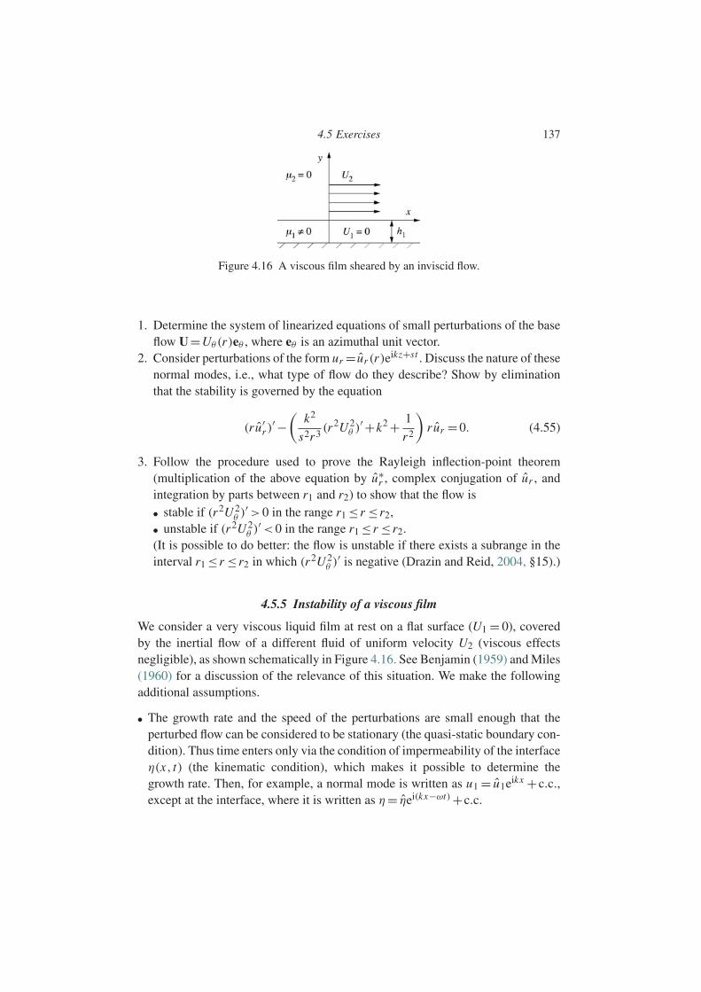
4.5 Exercises 137

Figure 4.16 A viscous film sheared by an inviscid flow.

1. Determine the system of linearized equations of small perturbations of the baseflow U=Uθ (r)eθ , where eθ is an azimuthal unit vector.

2. Consider perturbations of the form ur = ur (r)eikz+st . Discuss the nature of thesenormal modes, i.e., what type of flow do they describe? Show by eliminationthat the stability is governed by the equation

(r u′r )

′ −(

k2

s2r3(r2U 2

θ )′ +k2 + 1

r2

)r ur =0. (4.55)

3. Follow the procedure used to prove the Rayleigh inflection-point theorem(multiplication of the above equation by u∗

r , complex conjugation of ur , andintegration by parts between r1 and r2) to show that the flow is• stable if (r2U 2

θ )′ >0 in the range r1 ≤ r ≤ r2,

• unstable if (r2U 2θ )

′ <0 in the range r1 ≤ r ≤ r2.(It is possible to do better: the flow is unstable if there exists a subrange in theinterval r1 ≤ r ≤r2 in which (r2U 2

θ )′ is negative (Drazin and Reid, 2004, §15).)

4.5.5 Instability of a viscous film

We consider a very viscous liquid film at rest on a flat surface (U1 = 0), coveredby the inertial flow of a different fluid of uniform velocity U2 (viscous effectsnegligible), as shown schematically in Figure 4.16. See Benjamin (1959) and Miles(1960) for a discussion of the relevance of this situation. We make the followingadditional assumptions.

• The growth rate and the speed of the perturbations are small enough that theperturbed flow can be considered to be stationary (the quasi-static boundary con-dition). Thus time enters only via the condition of impermeability of the interfaceη(x, t) (the kinematic condition), which makes it possible to determine thegrowth rate. Then, for example, a normal mode is written as u1 = u1eikx +c.c.,except at the interface, where it is written as η= ηei(kx−ωt)+c.c.

138 Inviscid instability of parallel flows

• The perturbations in the inviscid fluid are irrotational.• The perturbations in the film are governed by the lubrication equations

0=−∂x p1 +µ1∂yyu1, 0=−∂y p1. (4.56)

• Surface tension and gravity can be neglected, except in the last question.

1. Determine the perturbation φ2 of the velocity potential and the perturbation p2

of the pressure in the inviscid fluid, up to a multiplicative constant A.2. Determine the flow u1 in the film as a function of p1 (after linearization at

the unperturbed interface y = 0 of the condition of zero tangential stress at theinterface). Next, use the incompressibility condition to determine the speed v1

in the film as a function of p1.3. Write down the linearized conditions for matching the normal velocities and the

normal forces at the interface (it will be shown that the normal forces reduce topressures). Find the velocity and pressure fields (up to a constant, since we aresolving a linear homogeneous problem).

4. Write down the kinematic condition at the interface (this equation is the onlyone which involves the time). Deduce the dispersion relation

ωτ = α3

α2 R −3i(4.57)

where α = kh1 is a dimensionless wave number, R = ρ2U2h1/µ1, and τ =µ1/ρ2U 2

2 is seen to be the characteristic time of the instability. Sketch the speedand the growth rate as functions of α. Discuss.

5. Include gravity g and surface tension γ in the analysis of a horizontal interface(the corresponding pressure field of the base is P1 = P0−ρ1gy, P2 = P0−ρ2gy,where P0 is the pressure at the interface). The study of the Rayleigh–Taylorinstability can be used as a guide. Sketch the speed and the growth rate asfunctions of α. Discuss.

5

Viscous instability of parallel flows

5.1 Introduction

The inertial instability of parallel flows described in the preceding chapter isassociated with the existence of an inflection point in the velocity profile. This isthe principal instability of parallel or quasi-parallel shear flows at large Reynoldsnumber and far from walls or interfaces, such as mixing layers, jets, and wakes.We have seen that the order of magnitude of the growth rate is U/δ, where U isthe difference of the speeds on either side of the vorticity layer of thickness δ,and that viscosity plays only a diffusive role tending to attenuate the growth rate.The instability of flow profiles without inflection points is profoundly different.Let us consider two fundamental flows: plane Poiseuille flow and boundary layerflow. Observation shows that plane Poiseuille flow is unstable beyond a certainReynolds number. Similarly, a boundary layer on a surface becomes unstable atsome distance from the leading edge. However, these two flows do not possessan inflection point, and so, ignoring viscosity, they are stable according to theRayleigh theorem. On the other hand, the growth rate of the observed instabilitiesis much smaller than would be expected for an inertial instability. It is thereforeclearly important to investigate the role played by viscosity, which is the goal of thepresent chapter. We shall see that viscosity has two effects: the expected stabilizingdissipative effect, and also a destabilizing effect. The latter, which unfortunatelyadmits no simple explanation, is due to a subtle coupling between inertia, viscouseffects near critical layers, and the no-slip condition.

We begin this chapter by presenting the two canonical situations where a vis-cous instability is manifested: plane Poiseuille flow and boundary layer flowon a flat surface (Section 5.1). We then display some general results (Section5.2) before returning to a more detailed study of Poiseuille flow (plane flow inSection 5.3 and pipe flow in Section 5.4) and boundary layer flows (Section 5.5).We also briefly discuss the phenomenon of the transient growth of particular

139

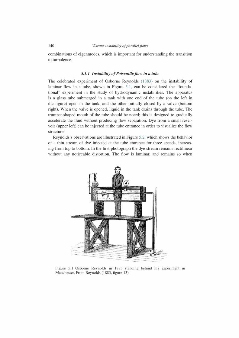
140 Viscous instability of parallel flows

combinations of eigenmodes, which is important for understanding the transitionto turbulence.

5.1.1 Instability of Poiseuille flow in a tube

The celebrated experiment of Osborne Reynolds (1883) on the instability oflaminar flow in a tube, shown in Figure 5.1, can be considered the “founda-tional” experiment in the study of hydrodynamic instabilities. The apparatusis a glass tube submerged in a tank with one end of the tube (on the left inthe figure) open in the tank, and the other initially closed by a valve (bottomright). When the valve is opened, liquid in the tank drains through the tube. Thetrumpet-shaped mouth of the tube should be noted; this is designed to graduallyaccelerate the fluid without producing flow separation. Dye from a small reser-voir (upper left) can be injected at the tube entrance in order to visualize the flowstructure.

Reynolds’s observations are illustrated in Figure 5.2, which shows the behaviorof a thin stream of dye injected at the tube entrance for three speeds, increas-ing from top to bottom. In the first photograph the dye stream remains rectilinearwithout any noticeable distortion. The flow is laminar, and remains so when

Figure 5.1 Osborne Reynolds in 1883 standing behind his experiment inManchester. From Reynolds (1883, figure 13)

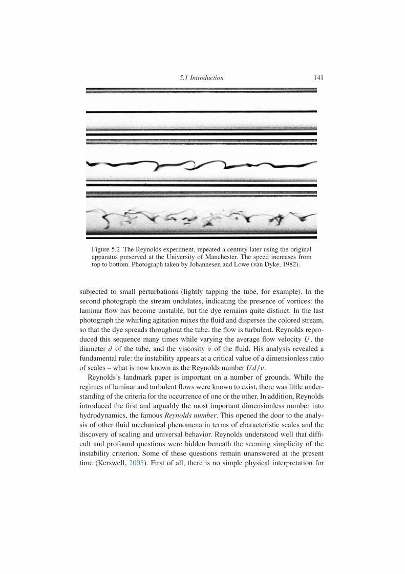
5.1 Introduction 141

Figure 5.2 The Reynolds experiment, repeated a century later using the originalapparatus preserved at the University of Manchester. The speed increases fromtop to bottom. Photograph taken by Johannesen and Lowe (van Dyke, 1982).

subjected to small perturbations (lightly tapping the tube, for example). In thesecond photograph the stream undulates, indicating the presence of vortices: thelaminar flow has become unstable, but the dye remains quite distinct. In the lastphotograph the whirling agitation mixes the fluid and disperses the colored stream,so that the dye spreads throughout the tube: the flow is turbulent. Reynolds repro-duced this sequence many times while varying the average flow velocity U , thediameter d of the tube, and the viscosity ν of the fluid. His analysis revealed afundamental rule: the instability appears at a critical value of a dimensionless ratioof scales – what is now known as the Reynolds number Ud/ν.

Reynolds’s landmark paper is important on a number of grounds. While theregimes of laminar and turbulent flows were known to exist, there was little under-standing of the criteria for the occurrence of one or the other. In addition, Reynoldsintroduced the first and arguably the most important dimensionless number intohydrodynamics, the famous Reynolds number. This opened the door to the analy-sis of other fluid mechanical phenomena in terms of characteristic scales and thediscovery of scaling and universal behavior. Reynolds understood well that diffi-cult and profound questions were hidden beneath the seeming simplicity of theinstability criterion. Some of these questions remain unanswered at the presenttime (Kerswell, 2005). First of all, there is no simple physical interpretation for

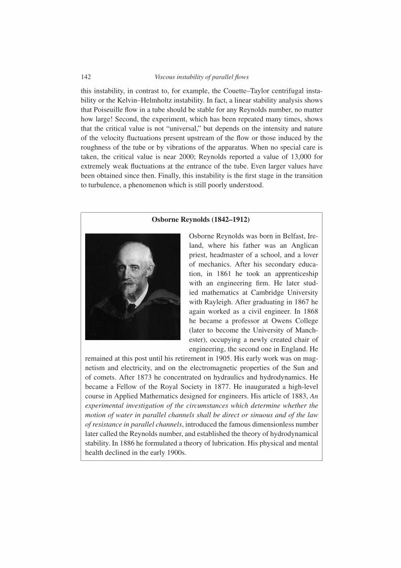
142 Viscous instability of parallel flows

this instability, in contrast to, for example, the Couette–Taylor centrifugal insta-bility or the Kelvin–Helmholtz instability. In fact, a linear stability analysis showsthat Poiseuille flow in a tube should be stable for any Reynolds number, no matterhow large! Second, the experiment, which has been repeated many times, showsthat the critical value is not “universal,” but depends on the intensity and natureof the velocity fluctuations present upstream of the flow or those induced by theroughness of the tube or by vibrations of the apparatus. When no special care istaken, the critical value is near 2000; Reynolds reported a value of 13,000 forextremely weak fluctuations at the entrance of the tube. Even larger values havebeen obtained since then. Finally, this instability is the first stage in the transitionto turbulence, a phenomenon which is still poorly understood.

Osborne Reynolds (1842–1912)

Osborne Reynolds was born in Belfast, Ire-land, where his father was an Anglicanpriest, headmaster of a school, and a loverof mechanics. After his secondary educa-tion, in 1861 he took an apprenticeshipwith an engineering firm. He later stud-ied mathematics at Cambridge Universitywith Rayleigh. After graduating in 1867 heagain worked as a civil engineer. In 1868he became a professor at Owens College(later to become the University of Manch-ester), occupying a newly created chair ofengineering, the second one in England. He

remained at this post until his retirement in 1905. His early work was on mag-netism and electricity, and on the electromagnetic properties of the Sun andof comets. After 1873 he concentrated on hydraulics and hydrodynamics. Hebecame a Fellow of the Royal Society in 1877. He inaugurated a high-levelcourse in Applied Mathematics designed for engineers. His article of 1883, Anexperimental investigation of the circumstances which determine whether themotion of water in parallel channels shall be direct or sinuous and of the lawof resistance in parallel channels, introduced the famous dimensionless numberlater called the Reynolds number, and established the theory of hydrodynamicalstability. In 1886 he formulated a theory of lubrication. His physical and mentalhealth declined in the early 1900s.

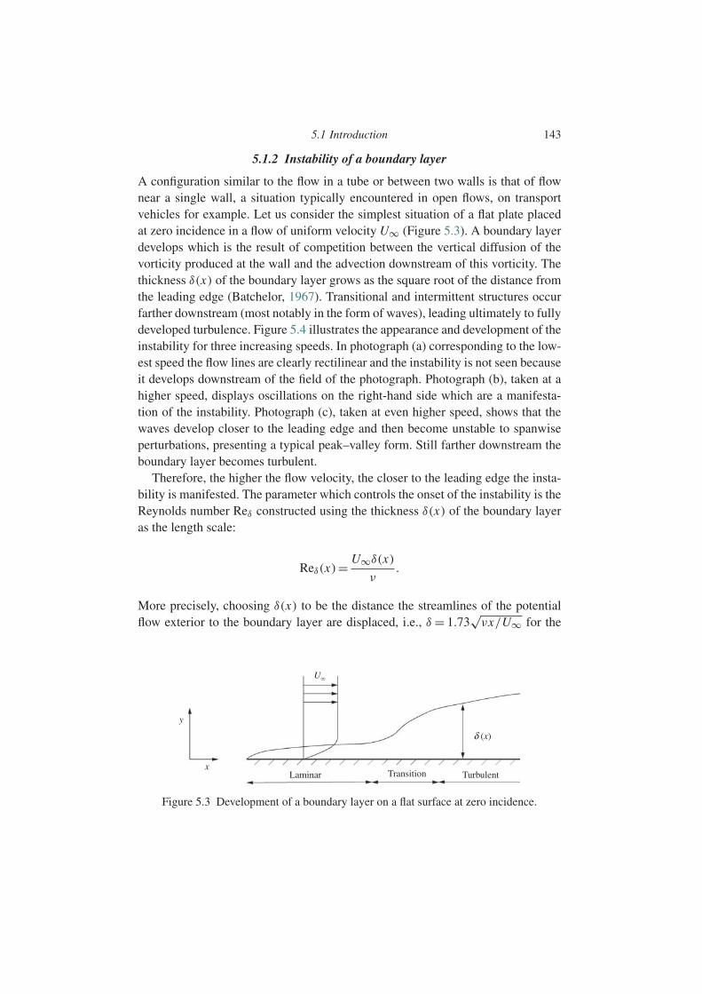
5.1 Introduction 143

5.1.2 Instability of a boundary layer

A configuration similar to the flow in a tube or between two walls is that of flownear a single wall, a situation typically encountered in open flows, on transportvehicles for example. Let us consider the simplest situation of a flat plate placedat zero incidence in a flow of uniform velocity U∞ (Figure 5.3). A boundary layerdevelops which is the result of competition between the vertical diffusion of thevorticity produced at the wall and the advection downstream of this vorticity. Thethickness δ(x) of the boundary layer grows as the square root of the distance fromthe leading edge (Batchelor, 1967). Transitional and intermittent structures occurfarther downstream (most notably in the form of waves), leading ultimately to fullydeveloped turbulence. Figure 5.4 illustrates the appearance and development of theinstability for three increasing speeds. In photograph (a) corresponding to the low-est speed the flow lines are clearly rectilinear and the instability is not seen becauseit develops downstream of the field of the photograph. Photograph (b), taken at ahigher speed, displays oscillations on the right-hand side which are a manifesta-tion of the instability. Photograph (c), taken at even higher speed, shows that thewaves develop closer to the leading edge and then become unstable to spanwiseperturbations, presenting a typical peak–valley form. Still farther downstream theboundary layer becomes turbulent.

Therefore, the higher the flow velocity, the closer to the leading edge the insta-bility is manifested. The parameter which controls the onset of the instability is theReynolds number Reδ constructed using the thickness δ(x) of the boundary layeras the length scale:

Reδ(x)= U∞δ(x)

ν.

More precisely, choosing δ(x) to be the distance the streamlines of the potentialflow exterior to the boundary layer are displaced, i.e., δ = 1.73

√νx/U∞ for the

Laminar Transition Turbulent

y

x

U

δ (x)

Figure 5.3 Development of a boundary layer on a flat surface at zero incidence.

144 Viscous instability of parallel flows

(a)

(b)

(c)

Figure 5.4 Flow lines on a boundary layer starting from the leading edge on theleft. The velocity increases in going from the top to the bottom photograph. (a)The instability is not visible; (b) Tollmien–Schlichting waves are seen; (c) thewaves now appear closer to the leading edge and then themselves become unstable(from Werle (1980), courtesy of ONERA).

Blasius boundary layer, the instability appears for Reδ,c =520 (or Rex =U∞x/ν≈90,000).

After the work by Prandtl (1921), who was the first to develop the idea of a vis-cous instability mechanism, these oscillations were predicted by Tollmien (1929)

5.2 General results 145

and Schlichting (1933), and since then have been known as Tollmien–Schlichtingwaves. The first experimental demonstration of the phenomenon was obtainedmuch later by Schubauer and Skramstad (1947). Since then, many studies havebeen devoted to this problem in connection with transportation engineering in par-ticular. Since turbulent friction is much higher than laminar friction, the overallfrictional drag force is weaker the farther downstream from the leading edge theinstability develops. Owing to the industrial and ecological requirements of reduc-ing friction (in order to reduce energy consumption and combustion gas emission),it is clearly important to have a good understanding of this instability. Unfortu-nately, its physical mechanism cannot be understood using dimensional analysis,as for Poiseuille flow.

5.2 General results

In this section we present some general results on the stability of viscous parallelflows. These include the basic linearized equations of the subject and the role ofnumerical analysis in their solution, an extension of the Squire theorem to includeviscous effects, and a discussion of the mechanism of viscous instability.

5.2.1 The linearized perturbation equations

We choose two characteristic scales L and V as our units of length and velocity,and ρV 2 as our unit of pressure. Defining the Reynolds number as Re = U L/ν,the incompressibility and Navier–Stokes equations can be written as

divU=0, (5.1)

∂t U+(U ·grad)U=−gradP + 1

ReU. (5.2)

Let U (y)ex and P be a parallel stationary solution of these equations, whichdefine the base flow. For example, for plane Poiseuille flow the base flowis U (y) = 1 − y2, taking as the length scale the half-distance between thewalls and as the velocity scale the maximum velocity. For the boundary layeron a flat plate the base flow U (y) is typically the Blasius solution of theboundary-layer equations (of course U (y) is only an approximate quasi-parallelflow solution of the full Navier–Stokes equations; this point will be discussedlater on).

We consider the perturbed flow (U+u, P + p) and linearize the equations forthe perturbations. This gives

146 Viscous instability of parallel flows

divu=0, (5.3)

(∂t +U∂x )u+v∂yU ex =−gradp+ 1

Reu. (5.4)

Since they are invariant under translations in x , z, and t (but not in y),these equations have a solution corresponding to normal modes proportional toei(kx x+kz z−ωt), with wave vector k = kx ex + kzez and frequency ω, as in the pre-ceding chapter. Therefore, these equations reduce to a system of homogeneousdifferential equations for the amplitudes u(y) and p(y):

ikx u +∂y v+ ikzw=0, (5.5a)

ikx (U −c)u +∂yU v=−ikx p+ 1

Re(∂yy −k2

x −k2z )u, (5.5b)

ikx (U −c)v=−∂y p+ 1

Re(∂yy −k2

x −k2z )v, (5.5c)

ikx (U −c)w=−ikz p+ 1

Re(∂yy −k2

x −k2z )w, (5.5d)

where c =ω/kx is the phase velocity of the perturbation in the direction x . Theboundary conditions correspond to no-slip on the walls for Poiseuille flow, andto no-slip on the wall at y = 0 and decay of the perturbations for y → ∞ forboundary-layer flow. The system (5.5) together with these conditions constitutes ageneralized eigenvalue problem which has nonzero solution only when the oper-ator is singular, that is, when the frequency ω and the wave vector k satisfy adispersion relation

D(k,ω,Re)=0. (5.6)

5.2.2 The Squire theorem

As for the inviscid flows of the preceding chapter, use of a transformation of vari-ables and a theorem due to Squire (1933) allows the three-dimensional problemto be reduced to an equivalent two-dimensional one. The Squire transformationconsists of introducing the same transformations defined in the preceding chapter:

k2 = k2x +k2

z , (5.7a)

ω= (k/kx )ω, (5.7b)

ku = kx u +kzw, (5.7c)

v= v, (5.7d)

p = (k/kx ) p, (5.7e)

5.2 General results 147

as well as an additional one:

kRe= kx Re. (5.8)

The system of four equations (5.5) is then replaced by the following system ofthree equations, with c = ω/k =ω/kx = c:

iku +∂y v=0, (5.9a)

ik(U − c)u +∂yU v=−ik p+ 1

Re(∂yy − k2)u, (5.9b)

ik(U − c)v=−∂y p+ 1

Re(∂yy − k2)v. (5.9c)

Associated with this system are the boundary conditions of decay at infinity,u, v → 0 for y → ∞, or no-slip at a solid surface, u(y1) = v(y1) = 0,u(y2) = v(y2) = 0. This homogeneous system of two-dimensional perturbationshas nonzero solution only if the following dispersion relation is satisfied:

D(k, ω, Re)=0. (5.10)

Once this relation is known, the three-dimensional dispersion relation can beobtained without further calculation by means of the Squire transformation:

D(k,ω;Re)= D

√k2x +k2

z ,

√k2

x +k2z

kxω; kx√

k2x +k2

z

Re

=0. (5.11)

From this expression we deduce the Squire theorem.

Theorem 5.1 With any unstable oblique mode (k,ω) of temporal growth rateωi for Reynolds number Re it is possible to associate a two-dimensional mode

(k, ω) of temporal growth rate ωi =ωi

√k2

x +k2z /kx , higher than ωi , at a Reynolds

number Re=Rekx/

√k2

x +k2z , lower than Re.

Corollary 5.2 If there exists a Reynolds number Rec above which a flow isunstable, the normal mode which destabilizes the flow for Re = Rec is two-dimensional. Indeed, if this were not the case, it would be possible to find anunstable two-dimensional mode for Re < Rec which contradicts the definitionof Rec.

If the problem is to determine an instability condition (typically, a criticalReynolds number), the Squire theorem states that it is sufficient to considertwo-dimensional perturbations. However, beyond the critical Reynolds number

148 Viscous instability of parallel flows

1.2

0.9

0.6

0.3

0.0

–0.3

–0.6

–0.9

–1.20 15 30

β (degrees)

103 ×

ωi

45 60 75

Figure 5.5 Temporal growth rate (s−1) of a boundary layer instability as a func-tion of the angle β of the perturbation relative to the direction of the base flow.Reδ =1500, ων/U 2∞ =0.3×10−4 (calculation by G. Casalis, ONERA).

(Re>Rec) the most unstable perturbation is not necessarily two-dimensional, butmay be oblique (kz = 0). This is illustrated in Figure 5.5, which shows the growthrate of a perturbation of the Blasius boundary layer as a function of the angleβ between the wave vector k and the direction of the base flow. For the Reynoldsnumber Reδ =1500 above the critical value Reδ,c =520 we see that the most unsta-ble perturbation is not two–dimensional (angle β equal to zero), but correspondsto an angle of about 50.

The Squire theorem was obtained above for rigid walls. It has been generalizedto the case of two or more fluid layers separated by a deformable interface, wherevelocity continuity and stress balance conditions must be satisfied (Hesla et al.,1986).

5.2.3 The Orr–Sommerfeld equation

Bearing in mind the Squire theorem, from now on we shall consider two-dimensional perturbations, and introduce the stream function ψ of the velocityperturbation defined as u = ∂yψ and v = −∂yψ . Eliminating the pressure bycross-differentiating the equations (5.4), we obtain

(∂t +U∂x )ψ −∂yyU∂xψ = 1

Re2ψ. (5.12)

This can also be recognized as the linearized transport equation for the vorticityperturbation ω=−ψ . Seeking the solution in the form of normal modes

5.2 General results 149

ψ(x, t)= 1

2ψ(y)ei(kx−ωt)+c.c.

of wave number k, frequency ω, and speed c =ω/k, we find the Orr–Sommerfeldequation (Orr, 1907; Sommerfeld, 1908):

(U −c)(∂yy −k2)ψ −∂yyU ψ = 1

ikRe(∂yy −k2)2ψ. (5.13)

The only difference between this equation and the Rayleigh equation (cf.Chapter 4) is the term on the right-hand side due to the viscous forces, whichraises the equation from second to fourth order (with the corresponding increasein the number of boundary conditions).

The associated boundary conditions are no-slip at the walls at y = y1 and y = y2,

∂yψ(y1)= ψ(y1)=0, (5.14a)

∂yψ(y2)= ψ(y2)=0, (5.14b)

or, in the case of a boundary layer on a wall at y = 0, the conditions of no-slip atthe wall and decay at large distances:

∂yψ = ψ =0 at y =0, (5.15a)

∂yψ, ψ →0 for y →∞, (5.15b)

or, finally, the conditions of velocity continuity and stress balance on a deformableinterface (in which case the speed also enters into the boundary conditions; cf.Chapter 6).

Writing the Orr–Sommerfeld equation as

L Aψ = c L Bψ,

where the differential operators L A and L B are defined as

L A = (∂yy −k2)2 − ikRe(

U (∂yy −k2)−∂yyU),

L B =−ikRe(∂yy −k2),

the problem becomes a generalized eigenvalue problem which has a nontrivialsolution only if the speed c satisfies a dispersion relation.

When temporal stability is studied, the problem is solved by imposing the con-dition that k is real, and then the complex speed is calculated; on the other hand,when spatial stability is studied, the condition of real frequency ω is imposed andthe wave numbers are calculated. For a given value of k or ω there exist in gen-eral several modes with different growth rates. Since the speed enters linearly into

150 Viscous instability of parallel flows

the problem (except possibly in the boundary conditions at a deformable interface)while the wave number enters quadratically, it is much easier to study temporal sta-bility than spatial stability, and generally it is the former that is considered whenseeking marginal stability conditions.

The Orr–Sommerfeld equation (5.13) is a fourth-order linear differentialequation with nonconstant coefficients. Exact solutions are known only in certainvery special cases, notably when ∂yyU = 0 (i.e., piecewise-linear velocity pro-files): the vorticity then satisfies an Airy equation, and the speed is expressed asintegrals of Airy functions (Exercise 5.6.3). For finite wave number and Reynoldsnumber the coefficient of the highest-order term (ikRe)−1 does not vanish, and theproblem of degeneracy of the Rayleigh equation for U = c (existence of a criti-cal layer) does not arise. However, when the instability appears at large Reynoldsnumber, which is the case in, for example, Poiseuille flow, the problem becomesdifficult to solve: the viscous term on the right-hand side, even though it has asmall coefficient, can become of the same order as the inertial terms in regionswhere the eigenfunction or its derivatives have large gradients. This happens, inparticular, near a wall and within the critical layer of the associated inviscid prob-lem, where the thickness of the region affected by viscosity is of order (kh Re)−1/2

and (kh Re)−1/3, respectively. Some imaginative and ingenious mathematical tech-niques have been developed, in particular, by Heisenberg (1924), Tollmien (1929),Schlichting (1933), and Lin (1955), to find solutions approached by asymptoticseries, or at least to determine an approximate marginal stability curve in the (k,Re) plane; see Drazin and Reid (2004, chapters 4 and 5). At small Reynolds num-ber or small wave number the asymptotic series are in general regular; an exampleis given in Chapter 6 for a liquid film flowing on an inclined plane.

Nowadays the Orr–Sommerfeld equation can be solved numerically withoutmuch difficulty. The numerical methods used most frequently are either shoot-ing or spectral methods (Canuto et al., 1988; Schmid and Henningson, 2001,appendix A). The former consists of spatially integrating the equation starting froma guess for the solution on one of the boundaries, integrating up to the other bound-ary, and then correcting the “trajectory” iteratively in order to satisfy the conditionson this other boundary. This method is easy to implement, but not very stable due tothe large spatial gradients alluded to above. Spectral methods consist of projectingthe amplitude ψ of the eigenfunction onto a basis of suitable functions φk(y):

ψ(y)=n∑

k=0

akφk(y), (5.17)

and solving for the coefficients ak in a manner consistent with the Orr–Sommerfeldequation. Choosing the functions φk(y) such that their derivatives are expressed as

5.2 General results 151

linear combinations of the functions themselves (like the trigonometric functions),the Orr–Sommerfeld equation and boundary conditions can be transformed intoa system of linear equations. The Chebyshev polynomials Tk(y) are a particu-larly appropriate basis1 because the collocation points cluster near the walls or theinterface, where the gradients of the eigenfunctions are in general large (Orszag,1971). Spectral (or pseudo-spectral, there are several variants) methods have theadvantage of being very precise and of giving approximations of the entire eigen-value spectrum (up to the order of the discretization), as well as of the associatedeigenfunctions.

We note that even though high-performance numerical methods are now readilyaccessible, asymptotic methods may still be needed for analyzing the behaviorof the solution near a singularity. Asymptotic methods are also very helpful inunderstanding the role played by the various parameters, as well as for gaining adeeper insight into the problem.

5.2.4 The viscous instability mechanism

As mentioned in Section 5.1, the viscous instability mechanism of a shear flownear a solid boundary or a deformable interface is not simple to describe. However,some understanding can be obtained from the equation for the kinetic energy of theperturbation, ek = 1

2(u2 +v2 +w2) per unit mass. Performing scalar multiplication

of the Navier–Stokes equation by the velocity perturbation vector and rearrangingit using divu=0, we find

(∂t +U∂x )ek +div((p+ek)u)=−∂yU (U +u)v+ 1

Re(div(u×ω)−ω ·ω),

(5.18)

where ω= rot(u) is the vorticity perturbation. Let us take a spatially periodic per-turbation with wavelength 2π/kx and 2π/kz in the x- and z-directions. Definingthe spatial average of a quantity q(x, y, z, t) as

〈q〉(y, t)= kx

2π

kz

2π

∫ 2π/kx

0

∫ 2π/kz

0q(x, y, z, t)dxdz (5.19)

1 The Chebyshev polynomials, defined as Tn(y)=cos(n cos−1(y)), form a basis on the interval [−1,1], to whicha more general integration range [y1, y2] or [0,∞] may be transformed by means of a change of variable. Thesepolynomials are related by the recursion relation T0 =1, T1 = y, Tn+1 =2yTn −Tn−1. Other recursion relationspermit the derivative of a polynomial to be expressed as a function of other polynomials, so that a differentialsystem can be transformed into an algebraic system.

152 Viscous instability of parallel flows

and noting that because of the boundary and periodicity conditions, 〈∂xq〉 =〈∂zq〉=0 and 〈v〉=0, the average of Eq. (5.18) can be written as

∂t 〈ek〉+∂y (〈pv〉+〈ekv〉)= ∂yU τxy + 1

Re∂y〈ωxw−ωzu〉− 1

Re〈ω ·ω〉, (5.20)

where τxy = −〈u v〉 is a Reynolds stress (Tritton, 1988, §19.3). Integrating thisequation between two walls at y1 and y2 and taking into account the no-slip condi-tions, we finally obtain the exact equation that holds for perturbations of arbitraryamplitude as

d

dt

∫ y2

y1

〈ek〉dy =∫ y2

y1

∂yUτxydy − 1

Re

∫ y2

y1

〈ω ·ω〉dy. (5.21)

This is a special version of the Reynolds–Orr equation (Lin, 1955; Drazin andReid, 2004, §53). The left-hand side represents the growth rate of the averagekinetic energy of the perturbation. If it is negative the base flow is stable, other-wise it is unstable. The second term on the right-hand side corresponds to viscousdissipation. It is always positive, and always tends to attenuate the perturbation.Therefore, only the first term can cause the perturbation to grow and will do so ifit dominates the dissipative term: this term corresponds to energy being “pumped”from the base flow into the perturbations.

We can also find an equation for the kinetic energy of an eigenmode startingfrom the linearized equations. We then obtain an equation identical to (5.21),because the contribution of the nonlinear advective term is in fact zero after inte-gration and application of the boundary and periodicity conditions. Let us thereforeconsider Eq. (5.21) for eigenmodes of the form

u = 1

2u(y)ei(kx−ωt)+c.c., u(y)=|u(y)|eiφu(y).

The Reynolds stress involved in the kinetic energy production term then becomes

τxy(y)=−1

2|u||v|cos(φu −φv)e

2ωi t . (5.22)

We note that this expression involves only the phase difference between u and v; itis only this difference which is physically meaningful, as the phases themselves areassociated with the arbitrary choice of origin (fixed, if needed, by a normalizationcondition for the eigenfunctions).

Let us neglect viscous dissipation for the time being. Since according to theRayleigh theorem a velocity profile without an inflection point is stable, the

5.2 General results 153

0.1 0.2 0.3 0.4 0.5 0.6y/h

0.7 0.8 0.9

y c =

0.8

732

1.0

τ xy

Figure 5.6 Transverse distribution of the Reynolds stress τxy (5.22) for planePoiseuille flow (the vertical scale, which is related to the normalization condition,is arbitrary). yc is the location of the critical layer where cr = U (yc). Re = 104,kh =1, and c =0.24+0.0037i. Taken from Stuart (1963).

eigenmodes are necessarily neutral, and the rate of variation of the kinetic energyis zero. On the other hand, for a neutral perturbation of an inviscid flow the com-ponents u and v of the velocity are exactly out of phase (Section 4.2.3), and sothe Reynolds stress (5.22) is zero. The kinetic energy production term is thereforezero, and Eq. (5.21) is satisfied trivially.

Let us now consider the effect of viscosity. Figure 5.6 shows a typical pro-file of the Reynolds stress τxy(y), corresponding to the unstable eigenmode ofplane Poiseuille flow (since this stress is antisymmetric [τxy(−y)=−τxy(y)], weshow it only in the half-plane). τxy(y) has the same sign as the gradient ∂yU ,and the kinetic energy production term is therefore positive. We see that theReynolds stress vanishes at the symmetry plane (y/h = 0), remains very weak upto y/h ≈ 0.8, has a sharp peak at y/h ≈ 0.9 located near the critical layer (wherethe speed of the eigenmode is equal to the flow speed), and then vanishes at thewall. Its higher value near the wall corresponds to a viscously-induced phase shiftbetween u and v, which is related to a combination of viscous effects near the crit-ical layer and those near the wall due to the no-slip condition (see also Figures 5.8and 5.10 below).

Therefore, at small Reynolds number the production of kinetic energy is smallerthan the dissipation, and the flow is stable. However, at large Reynolds numberdissipation becomes negligible (measured on the characteristic scales of the flow hand U (0)), and production dominates, making the flow unstable. Viscous diffusiontherefore has two effects: a stabilizing effect via the dissipation term, and a destabi-lizing effect related to the no-slip condition which distorts the phase angle betweenu and v. A similar situation can arise near a deformable interface. This discussiondoes not really explain the instability, but it does nevertheless shed some light on

154 Viscous instability of parallel flows

the subtle and delicate role played by viscosity near a wall. Note finally that amechanism has been proposed by Baines et al. (1996) for the growth of Tollmien–Schlichting waves, based on a linear resonance between an inviscid mode and aviscous mode; see Exercise 5.6.4.

5.3 Plane Poiseuille flow

5.3.1 Marginal stability, eigenmodes

Plane Poiseuille flow is typical of a parallel flow being unstable beyond a criticalReynolds number, when the production of kinetic energy of small perturbations,associated with the Reynolds stress τxy , exceeds the viscous dissipation. Thecontrol parameter of this instability is the Reynolds number

Re= Uh

ν, (5.23)

where U is the speed in the center of the channel, h is the half-height of thechannel, and ν is the kinematic viscosity. Figure 5.7 shows the marginal stabil-ity curve obtained by solving the Orr–Sommerfeld equation. For Rec = 5772 theflow becomes unstable to a perturbation of wave number kch =1.02. Near thresh-old the curve is parabolic and the width of the band of unstable wave numbersgrows as

√Re−Rec. At large Reynolds number this unstable band shifts toward

zero (long wavelengths) and becomes narrower. It can be shown that the upperbranch behaves as Re∼ (kh)−11, and that the two regions affected by the viscosity,

kch

ωi < 0 ωi > 0

kh

Re ~ (kh)–11

Re ~ (kh)–7

Rec Re

Figure 5.7 Shape of the marginal stability curve in the Re−kh plane for planePoiseuille flow.

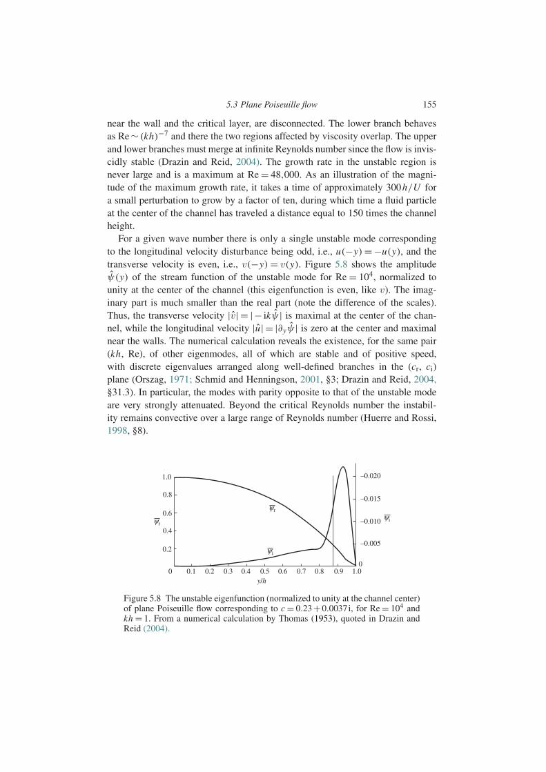
5.3 Plane Poiseuille flow 155

near the wall and the critical layer, are disconnected. The lower branch behavesas Re∼ (kh)−7 and there the two regions affected by viscosity overlap. The upperand lower branches must merge at infinite Reynolds number since the flow is invis-cidly stable (Drazin and Reid, 2004). The growth rate in the unstable region isnever large and is a maximum at Re = 48,000. As an illustration of the magni-tude of the maximum growth rate, it takes a time of approximately 300h/U fora small perturbation to grow by a factor of ten, during which time a fluid particleat the center of the channel has traveled a distance equal to 150 times the channelheight.

For a given wave number there is only a single unstable mode correspondingto the longitudinal velocity disturbance being odd, i.e., u(−y)= −u(y), and thetransverse velocity is even, i.e., v(−y) = v(y). Figure 5.8 shows the amplitudeψ(y) of the stream function of the unstable mode for Re = 104, normalized tounity at the center of the channel (this eigenfunction is even, like v). The imag-inary part is much smaller than the real part (note the difference of the scales).Thus, the transverse velocity |v| = |− ikψ | is maximal at the center of the chan-nel, while the longitudinal velocity |u| = |∂yψ | is zero at the center and maximalnear the walls. The numerical calculation reveals the existence, for the same pair(kh, Re), of other eigenmodes, all of which are stable and of positive speed,with discrete eigenvalues arranged along well-defined branches in the (cr, ci)plane (Orszag, 1971; Schmid and Henningson, 2001, §3; Drazin and Reid, 2004,§31.3). In particular, the modes with parity opposite to that of the unstable modeare very strongly attenuated. Beyond the critical Reynolds number the instabil-ity remains convective over a large range of Reynolds number (Huerre and Rossi,1998, §8).

1.0

0.8

0.6

0.4

0.2

0 0.1 0.2 0.3 0.4 0.5y/h

ψr

0.6 0.7 0.8 0.9 1.00

–0.005

–0.010

–0.015

–0.020

ψr

ψi

ψi

Figure 5.8 The unstable eigenfunction (normalized to unity at the channel center)of plane Poiseuille flow corresponding to c = 0.23+0.0037i, for Re = 104 andkh = 1. From a numerical calculation by Thomas (1953), quoted in Drazin andReid (2004).

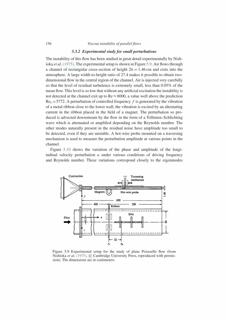
156 Viscous instability of parallel flows

5.3.2 Experimental study for small perturbations

The instability of this flow has been studied in great detail experimentally by Nish-ioka et al. (1975). The experimental setup is shown in Figure 5.9. Air flows througha channel of rectangular cross-section of height 2h = 1.46 cm and exits into theatmosphere. A large width-to-height ratio of 27.4 makes it possible to obtain two-dimensional flow in the central region of the channel. Air is injected very carefullyso that the level of residual turbulence is extremely small, less than 0.05% of themean flow. This level is so low that without any artificial excitation the instability isnot detected at the channel exit up to Re≈8000, a value well above the predictionRec =5772. A perturbation of controlled frequency f is generated by the vibrationof a metal ribbon close to the lower wall; the vibration is excited by an alternatingcurrent in the ribbon placed in the field of a magnet. The perturbation so pro-duced is advected downstream by the flow in the form of a Tollmien–Schlichtingwave which is attenuated or amplified depending on the Reynolds number. Theother modes naturally present in the residual noise have amplitude too small tobe detected, even if they are unstable. A hot-wire probe mounted on a traversingmechanism is used to measure the perturbation amplitude at various points in thechannel.

Figure 5.10 shows the variation of the phase and amplitude of the longi-tudinal velocity perturbation u under various conditions of driving frequencyand Reynolds number. These variations correspond closely to the eigenmodes

Figure 5.9 Experimental setup for the study of plane Poiseuille flow (fromNishioka et al. (1975), c© Cambridge University Press, reproduced with permis-sion). The dimensions are in centimeters.

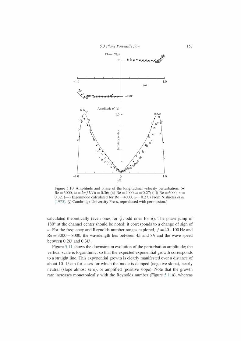
5.3 Plane Poiseuille flow 157

1.0

–1.0

Phase θ (y)

1.0

0°

–180°

–1.0 0 1.0

(arb

itary

sca

le)

y/h

y/h

Amplitude u (y)

Figure 5.10 Amplitude and phase of the longitudinal velocity perturbation: (•)Re = 3000, ω = 2π f U/h = 0.36; () Re = 4000,ω = 0.27; () Re = 6000, ω =0.32. (—) Eigenmode calculated for Re = 4000, ω= 0.27. (From Nishioka et al.(1975), c© Cambridge University Press, reproduced with permission.)

calculated theoretically (even ones for ψ , odd ones for u). The phase jump of180 at the channel center should be noted; it corresponds to a change of sign ofu. For the frequency and Reynolds number ranges explored, f = 40−100 Hz andRe = 3000 − 8000, the wavelength lies between 4h and 8h and the wave speedbetween 0.2U and 0.3U .

Figure 5.11 shows the downstream evolution of the perturbation amplitude; thevertical scale is logarithmic, so that the expected exponential growth correspondsto a straight line. This exponential growth is clearly manifested over a distance ofabout 10–15 cm for cases for which the mode is damped (negative slope), nearlyneutral (slope almost zero), or amplified (positive slope). Note that the growthrate increases monotonically with the Reynolds number (Figure 5.11a), whereas

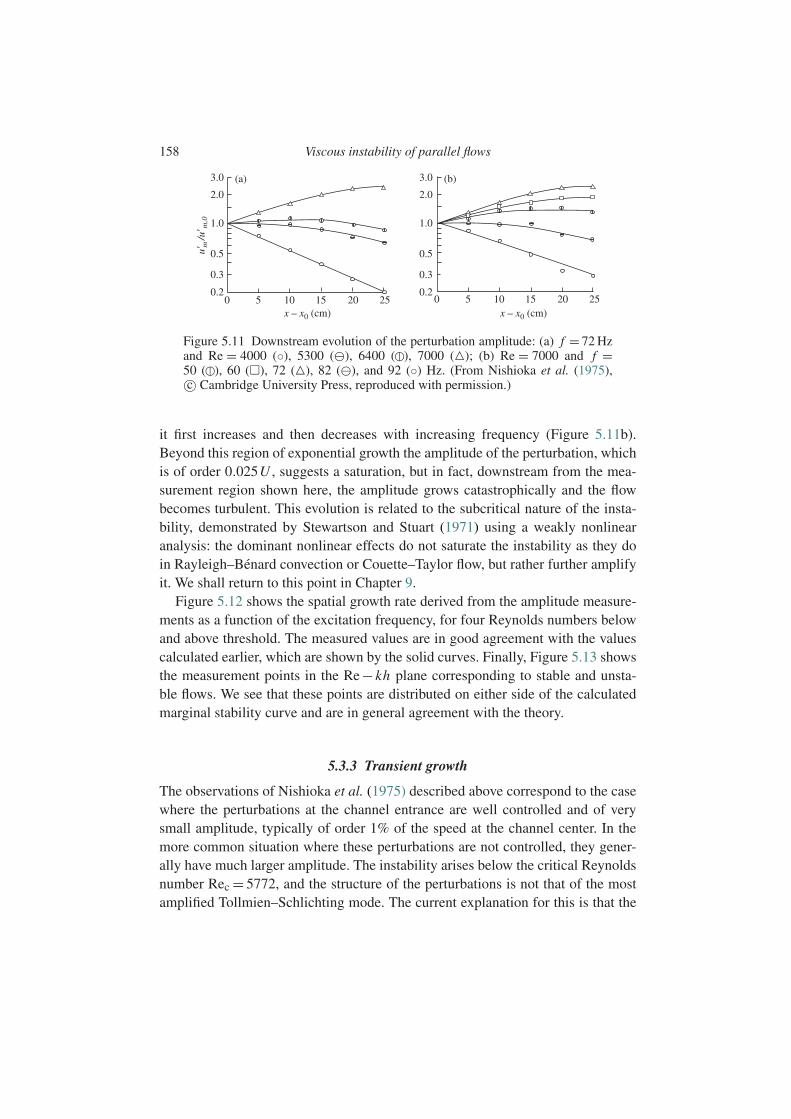
158 Viscous instability of parallel flows

3.0 (a) (b)

2.0

1.0

0.5

0.3

0.2

3.0

2.0

1.0

0.5

0.3

0.20 5 10 15

x – x0 (cm)

um

/u m

,0

x – x0 (cm)20 25 0 5 10 15 20 25

Figure 5.11 Downstream evolution of the perturbation amplitude: (a) f = 72 Hzand Re = 4000 (), 5300 (!), 6400 ( !), 7000 ("); (b) Re = 7000 and f =50 ( !), 60 (), 72 ("), 82 (!), and 92 () Hz. (From Nishioka et al. (1975),c© Cambridge University Press, reproduced with permission.)

it first increases and then decreases with increasing frequency (Figure 5.11b).Beyond this region of exponential growth the amplitude of the perturbation, whichis of order 0.025U , suggests a saturation, but in fact, downstream from the mea-surement region shown here, the amplitude grows catastrophically and the flowbecomes turbulent. This evolution is related to the subcritical nature of the insta-bility, demonstrated by Stewartson and Stuart (1971) using a weakly nonlinearanalysis: the dominant nonlinear effects do not saturate the instability as they doin Rayleigh–Benard convection or Couette–Taylor flow, but rather further amplifyit. We shall return to this point in Chapter 9.

Figure 5.12 shows the spatial growth rate derived from the amplitude measure-ments as a function of the excitation frequency, for four Reynolds numbers belowand above threshold. The measured values are in good agreement with the valuescalculated earlier, which are shown by the solid curves. Finally, Figure 5.13 showsthe measurement points in the Re− kh plane corresponding to stable and unsta-ble flows. We see that these points are distributed on either side of the calculatedmarginal stability curve and are in general agreement with the theory.

5.3.3 Transient growth

The observations of Nishioka et al. (1975) described above correspond to the casewhere the perturbations at the channel entrance are well controlled and of verysmall amplitude, typically of order 1% of the speed at the channel center. In themore common situation where these perturbations are not controlled, they gener-ally have much larger amplitude. The instability arises below the critical Reynoldsnumber Rec = 5772, and the structure of the perturbations is not that of the mostamplified Tollmien–Schlichting mode. The current explanation for this is that the

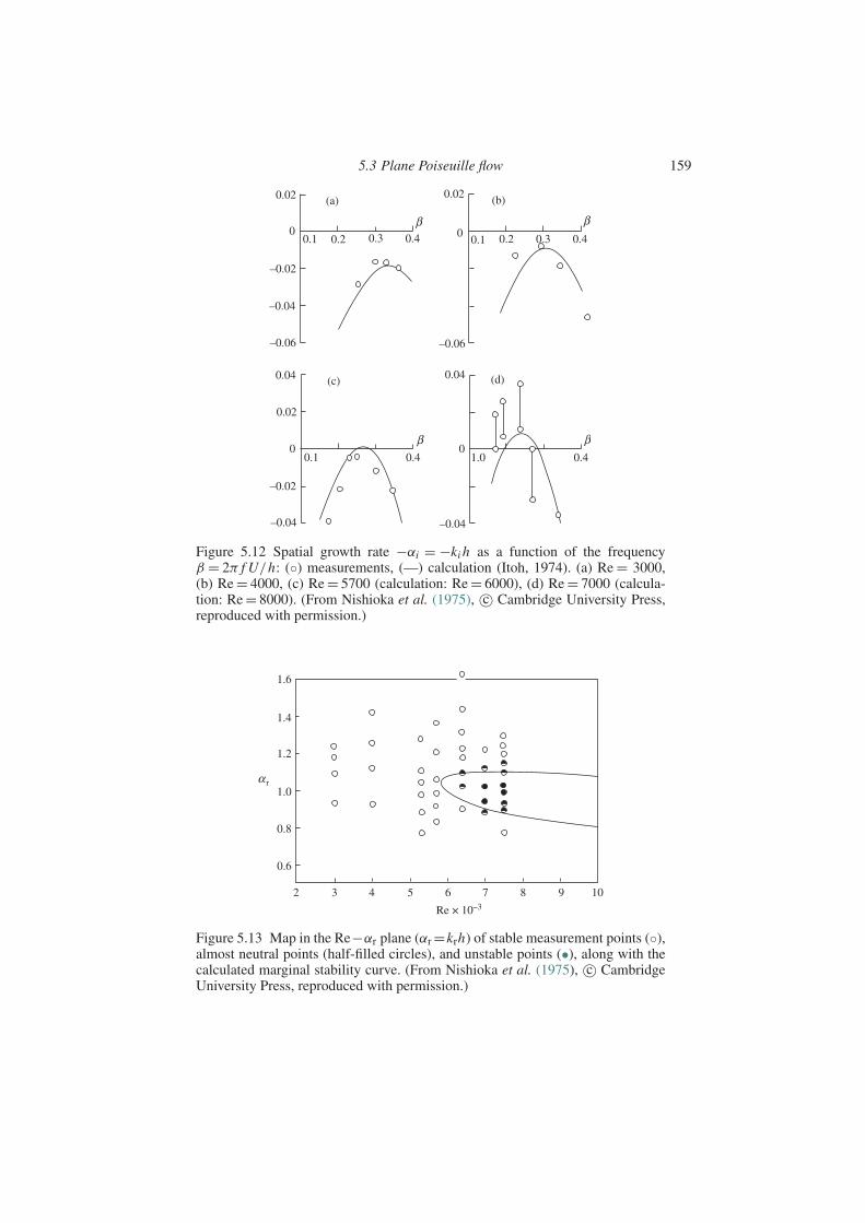
5.3 Plane Poiseuille flow 159

0.02 0.02

–0.06

0.04

(a) (b)

(c) (d)

0.02

–0.02

–0.04

00.1

0.1 0.2 0.3 0.4 0.40.30.20.1

1.0 0.40.4

0 0

–0.02

–0.04

–0.06

0.04

–0.04

0

β β

ββ

Figure 5.12 Spatial growth rate −αi = −ki h as a function of the frequencyβ = 2π f U/h: () measurements, (—) calculation (Itoh, 1974). (a) Re = 3000,(b) Re = 4000, (c) Re = 5700 (calculation: Re = 6000), (d) Re = 7000 (calcula-tion: Re = 8000). (From Nishioka et al. (1975), c© Cambridge University Press,reproduced with permission.)

2 3 4 5 6

Re × 10–3

7 8 9 10

1.6

1.4

1.2

1.0α r

0.8

0.6

Figure 5.13 Map in the Re−αr plane (αr =krh) of stable measurement points (),almost neutral points (half-filled circles), and unstable points (•), along with thecalculated marginal stability curve. (From Nishioka et al. (1975), c© CambridgeUniversity Press, reproduced with permission.)

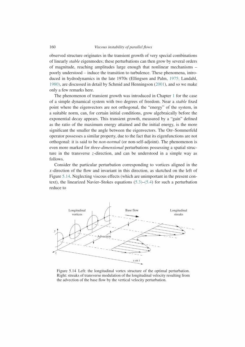
160 Viscous instability of parallel flows

observed structure originates in the transient growth of very special combinationsof linearly stable eigenmodes; these perturbations can then grow by several ordersof magnitude, reaching amplitudes large enough that nonlinear mechanisms –poorly understood – induce the transition to turbulence. These phenomena, intro-duced in hydrodynamics in the late 1970s (Ellingsen and Palm, 1975; Landahl,1980), are discussed in detail by Schmid and Henningson (2001), and so we makeonly a few remarks here.

The phenomenon of transient growth was introduced in Chapter 1 for the caseof a simple dynamical system with two degrees of freedom. Near a stable fixedpoint where the eigenvectors are not orthogonal, the “energy” of the system, ina suitable norm, can, for certain initial conditions, grow algebraically before theexponential decay appears. This transient growth, measured by a “gain” definedas the ratio of the maximum energy attained and the initial energy, is the moresignificant the smaller the angle between the eigenvectors. The Orr–Sommerfeldoperator possesses a similar property, due to the fact that its eigenfunctions are notorthogonal: it is said to be non-normal (or non-self-adjoint). The phenomenon iseven more marked for three-dimensional perturbations possessing a spatial struc-ture in the transverse z-direction, and can be understood in a simple way asfollows.

Consider the particular perturbation corresponding to vortices aligned in thex-direction of the flow and invariant in this direction, as sketched on the left ofFigure 5.14. Neglecting viscous effects (which are unimportant in the present con-text), the linearized Navier–Stokes equations (5.3)–(5.4) for such a perturbationreduce to

Longitudinalvortices

Base flow

x or t

Advection

Longitudinalstreaks

y

z

Figure 5.14 Left: the longitudinal vortex structure of the optimal perturbation.Right: streaks of transverse modulation of the longitudinal velocity resulting fromthe advection of the base flow by the vertical velocity perturbation.

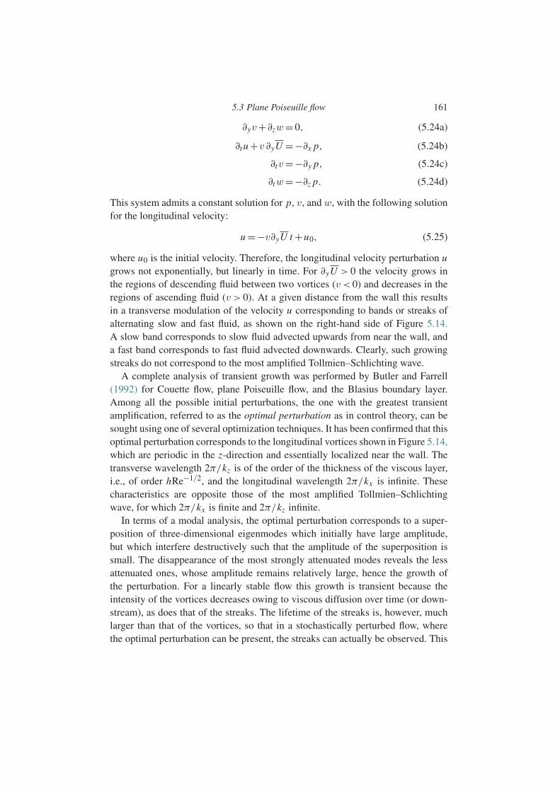
5.3 Plane Poiseuille flow 161

∂yv+∂zw=0, (5.24a)

∂t u +v ∂yU =−∂x p, (5.24b)

∂tv=−∂y p, (5.24c)

∂tw=−∂z p. (5.24d)

This system admits a constant solution for p, v, and w, with the following solutionfor the longitudinal velocity:

u =−v∂yU t +u0, (5.25)

where u0 is the initial velocity. Therefore, the longitudinal velocity perturbation ugrows not exponentially, but linearly in time. For ∂yU > 0 the velocity grows inthe regions of descending fluid between two vortices (v< 0) and decreases in theregions of ascending fluid (v> 0). At a given distance from the wall this resultsin a transverse modulation of the velocity u corresponding to bands or streaks ofalternating slow and fast fluid, as shown on the right-hand side of Figure 5.14.A slow band corresponds to slow fluid advected upwards from near the wall, anda fast band corresponds to fast fluid advected downwards. Clearly, such growingstreaks do not correspond to the most amplified Tollmien–Schlichting wave.

A complete analysis of transient growth was performed by Butler and Farrell(1992) for Couette flow, plane Poiseuille flow, and the Blasius boundary layer.Among all the possible initial perturbations, the one with the greatest transientamplification, referred to as the optimal perturbation as in control theory, can besought using one of several optimization techniques. It has been confirmed that thisoptimal perturbation corresponds to the longitudinal vortices shown in Figure 5.14,which are periodic in the z-direction and essentially localized near the wall. Thetransverse wavelength 2π/kz is of the order of the thickness of the viscous layer,i.e., of order hRe−1/2, and the longitudinal wavelength 2π/kx is infinite. Thesecharacteristics are opposite those of the most amplified Tollmien–Schlichtingwave, for which 2π/kx is finite and 2π/kz infinite.

In terms of a modal analysis, the optimal perturbation corresponds to a super-position of three-dimensional eigenmodes which initially have large amplitude,but which interfere destructively such that the amplitude of the superposition issmall. The disappearance of the most strongly attenuated modes reveals the lessattenuated ones, whose amplitude remains relatively large, hence the growth ofthe perturbation. For a linearly stable flow this growth is transient because theintensity of the vortices decreases owing to viscous diffusion over time (or down-stream), as does that of the streaks. The lifetime of the streaks is, however, muchlarger than that of the vortices, so that in a stochastically perturbed flow, wherethe optimal perturbation can be present, the streaks can actually be observed. This

162 Viscous instability of parallel flows

has been confirmed by numerical simulations (Luchini, 2000). We finally note thataccording to the Squire theorem, any three-dimensional perturbation must decreasebelow the instability threshold of two-dimensional perturbations in the sense ofasymptotic stability. The result that a three-dimensional perturbation grows in atransient manner faster than a two-dimensional perturbation does not contradictthis theorem.

5.4 Poiseuille flow in a pipe

Poiseuille flow in a circular pipe is linearly stable for any Reynolds number, incontrast with plane Poiseuille flow. This surprising result, arrived at graduallybetween the 1920s and the 1960s when numerical computation came into use,seems to contradict the observations of Reynolds described at the beginning ofthis chapter, namely, destabilization at Reynolds numbers near 2000. This paradoxstill has not been fully understood (Kerswell, 2005), but several recently identifiedphenomena may help resolve it, i.e., (i) the phenomenon of advection normal tothe wall of the longitudinal momentum by longitudinal vortices, as in planar flow,and (ii) nonlinear effects corresponding to a subcritical bifurcation which amplifythe perturbations when their amplitude becomes sufficiently large. The transitionto turbulence in plane Couette flow, which is also linearly stable for any Reynoldsnumber even though a transition to turbulence is observed for Rec ≈ 350, mayinvolve the same phenomena. We shall return to this subject in Chapter 9.

5.5 Boundary layer on a flat surface

5.5.1 Experimental demonstration

The instability of a laminar boundary layer is a convective instability with a mech-anism very similar to that of plane Poiseuille flow. However, there is a differencein that the former develops from an inhomogeneous (translationally noninvariant)flow in the flow direction. The spatial development of the instability is shown inFigure 5.15, which shows time recordings of a Tollmien–Schlichting wave forcedupstream by the vibration of a ribbon at various distances from the leading edge(Schubauer and Skramstad, 1947). The rate of residual turbulence of the inci-dent flow, below 0.05%, is extremely small, as in the experiments of Nishiokaet al. (1975) on plane Poiseuille flow. The forcing frequency f is such that thedimensionless number

F = ων

U 2∞, ω=2π f (5.26)

5.5 Boundary layer on a flat surface 163

8

9

9.5

10

10.5

Figure 5.15 Velocity fluctuations in a boundary layer of a forced Tollmien–Schlichting wave, measured at different positions (in feet) downstream fromthe leading edge, for an upstream velocity U∞ = 36.6 m s−1 (Schubauer andSkramstad, 19472).

is of order 10−4. The velocity fluctuations are measured by hot-wire anemometry.We see that the wave is nearly linear (sinusoidal) in the first three recordings, upto a long-wavelength modulation, and then it rapidly becomes disordered owing tononlinear effects preceding turbulence. The wavelength is of order 104 ν/U∞, i.e.,a centimeter in air.

5.5.2 Local analysis

Theoretical study of boundary layer instability is complicated by the fact thatsince the boundary layer gets thicker downstream, the flow is not strictly paral-lel, especially near the leading edge where the Reynolds number is not very high(Section 5.1.2). This problem can be evaded by assuming that the x-gradient ofthe base flow is sufficiently small compared to the wave number of the perturba-tion, and that the characteristics of this perturbation (its amplitude, wave number,growth rate) adapt rapidly to the new local conditions encountered as a result ofits advection downstream. This hypothesis of rapid relaxation or “fully developedperturbation” makes it possible to use a local stability analysis, where the x-gradients of the base flow are assumed to be zero. The problem then becomes thatof the Orr–Sommerfeld equation for the parallel velocity profile U (x, y), wherethe x-coordinate is treated as a parameter. The growth rates, wavelengths, andeigenfunctions calculated in this way are then parametric functions of x .

The spatial evolution of the amplitude of an eigenmode of a given frequencyis affected by the nonuniformity of the base velocity profile in the flow direction.

2 Official contribution of the National Institute of Standards and Technology; not subject to copyright in theUnited States.

164 Viscous instability of parallel flows

Using the “fully developed perturbation” hypothesis, this amplitude is obtainedby integrating the local growth rate −ki (x) starting from the amplitude a0 at thepoint x0:

a(x)=a0 exp

(−∫ x

x0

ki (ξ)dξ

). (5.27)

Since the local growth rate −ki (x) is not spatially uniform, this amplitude does notvary exponentially with downstream distance, in contrast with a strictly parallelflow.

5.5.3 Eigenmodes, marginal stability, and nonparallel effects

Figure 5.16 shows the Blasius velocity profile of the base flow, both measuredand calculated, as well as an eigenmode of the velocity perturbation u measuredand calculated using the local analysis. This particular eigenmode was isolatedby the vibration of a ribbon close to the wall in a flow with very low noise.

10 u(y)/umax

Dis

tanc

e fr

om th

e w

all (

mm

)

8

6

4

2

00 0.2 0.4 0.6 0.8 1.0

U(y)/U`

Figure 5.16 Base flow and eigenfunction u′(y)=|u(y)| of the Blasius boundarylayer: (—) calculation, (, •) measurements. Used with permission of AnnualReviews, Inc., from Reed et al. (1996); permission conveyed through CopyrightClearance Center, Inc.

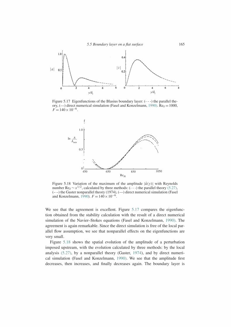
5.5 Boundary layer on a flat surface 165

û

y/δ1y/δ1

v

Figure 5.17 Eigenfunctions of the Blasius boundary layer: (- - -) the parallel the-ory, (—) direct numerical simulation (Fasel and Konzelmann, 1990). Reδ =1000,F =140×10−6.

1.0

0.5

In

Reδ1

0450 650 850 1050

A Amin

Figure 5.18 Variation of the maximum of the amplitude |u(y)| with Reynoldsnumber Reδ ∼ x1/2, calculated by three methods: (- - -) the parallel theory (5.27),(– –) the Gaster nonparallel theory (1974), (—) direct numerical simulation (Faseland Konzelmann, 1990). F =140×10−6.

We see that the agreement is excellent. Figure 5.17 compares the eigenfunc-tion obtained from the stability calculation with the result of a direct numericalsimulation of the Navier–Stokes equations (Fasel and Konzelmann, 1990). Theagreement is again remarkable. Since the direct simulation is free of the local par-allel flow assumption, we see that nonparallel effects on the eigenfunctions arevery small.

Figure 5.18 shows the spatial evolution of the amplitude of a perturbationimposed upstream, with the evolution calculated by three methods: by the localanalysis (5.27), by a nonparallel theory (Gaster, 1974), and by direct numeri-cal simulation (Fasel and Konzelmann, 1990). We see that the amplitude firstdecreases, then increases, and finally decreases again. The boundary layer is

166 Viscous instability of parallel flows

3

2

1

0 400 600

Reδ

F × 104

800

α i = 0.000 28

Figure 5.19 Marginal stability of the boundary layer on a flat surface: (—) theparallel theory, (– –) the nonparallel theory of Gaster (1974), (•) direct numericalsimulations of Fasel and Konzelmann (1990).

therefore first stable, then unstable, and then again stable. The band of unstableReynolds numbers lies between the minimum and maximum amplitude. Mea-surements display a similar evolution (Ross et al., 1970), as long as nonlinearor three-dimensional effects remain negligible even when the perturbation reachesits maximum amplitude.

The marginal stability curve in the Reδ − F plane can be obtained from the spa-tial evolution of a perturbation for various frequencies. This is shown in Figure5.19, for the three different approaches. The “half-banana” shape corresponds tothe restabilization of a wave packet of a given frequency. Such a packet is repre-sented by a point which moves to the right on a line F = constant. The packet is atfirst stable until it reaches the left-hand branch (called I) of the marginal curve, thenunstable until it reaches the right-hand branch (II), after which it is again stable.Theoretical and numerical results are compared with the measurements of Ross etal. (1970) in Figure 5.20. We see from these figures that the parallel theory givesgood results for Reδ > 600, but that significant nonparallel effects are manifestedfor Reδ <600.

The first calculation of a marginal stability curve (not shown in Figure 5.19)was done by Tollmien (1929) well before the first measurements of Schubauer

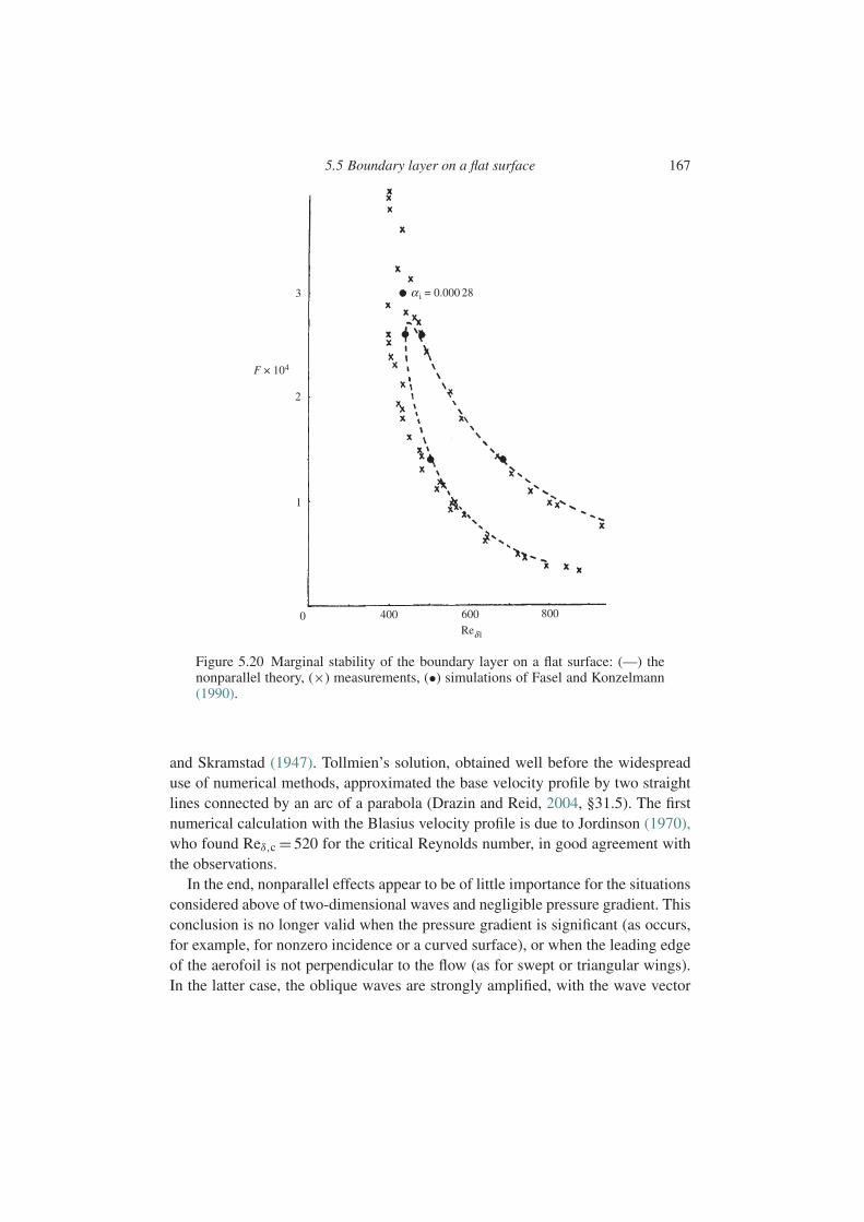
5.5 Boundary layer on a flat surface 167

3

2

1

0 400 600 800

Reδ1

F × 104

α i = 0.000 28

Figure 5.20 Marginal stability of the boundary layer on a flat surface: (—) thenonparallel theory, (×) measurements, (•) simulations of Fasel and Konzelmann(1990).

and Skramstad (1947). Tollmien’s solution, obtained well before the widespreaduse of numerical methods, approximated the base velocity profile by two straightlines connected by an arc of a parabola (Drazin and Reid, 2004, §31.5). The firstnumerical calculation with the Blasius velocity profile is due to Jordinson (1970),who found Reδ,c = 520 for the critical Reynolds number, in good agreement withthe observations.

In the end, nonparallel effects appear to be of little importance for the situationsconsidered above of two-dimensional waves and negligible pressure gradient. Thisconclusion is no longer valid when the pressure gradient is significant (as occurs,for example, for nonzero incidence or a curved surface), or when the leading edgeof the aerofoil is not perpendicular to the flow (as for swept or triangular wings).In the latter case, the oblique waves are strongly amplified, with the wave vector

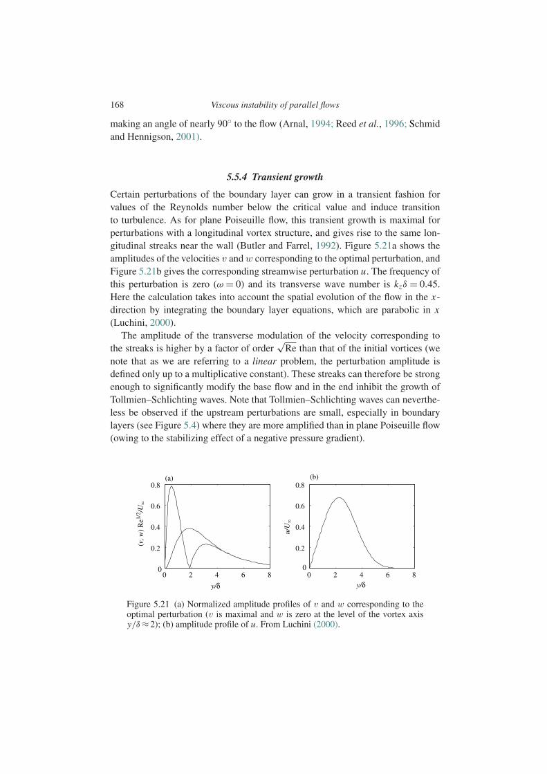
168 Viscous instability of parallel flows

making an angle of nearly 90 to the flow (Arnal, 1994; Reed et al., 1996; Schmidand Hennigson, 2001).

5.5.4 Transient growth

Certain perturbations of the boundary layer can grow in a transient fashion forvalues of the Reynolds number below the critical value and induce transitionto turbulence. As for plane Poiseuille flow, this transient growth is maximal forperturbations with a longitudinal vortex structure, and gives rise to the same lon-gitudinal streaks near the wall (Butler and Farrel, 1992). Figure 5.21a shows theamplitudes of the velocities v and w corresponding to the optimal perturbation, andFigure 5.21b gives the corresponding streamwise perturbation u. The frequency ofthis perturbation is zero (ω = 0) and its transverse wave number is kzδ = 0.45.Here the calculation takes into account the spatial evolution of the flow in the x-direction by integrating the boundary layer equations, which are parabolic in x(Luchini, 2000).

The amplitude of the transverse modulation of the velocity corresponding tothe streaks is higher by a factor of order

√Re than that of the initial vortices (we

note that as we are referring to a linear problem, the perturbation amplitude isdefined only up to a multiplicative constant). These streaks can therefore be strongenough to significantly modify the base flow and in the end inhibit the growth ofTollmien–Schlichting waves. Note that Tollmien–Schlichting waves can neverthe-less be observed if the upstream perturbations are small, especially in boundarylayers (see Figure 5.4) where they are more amplified than in plane Poiseuille flow(owing to the stabilizing effect of a negative pressure gradient).

0 2 4 6 80

0.2

0.4

0.6

0.8(a) (b)

y/δ

(v,

w)

Re1/

2 /U

0 2 4 6 80

0.2

0.4

0.6

0.8

y/δ

u/U

Figure 5.21 (a) Normalized amplitude profiles of v and w corresponding to theoptimal perturbation (v is maximal and w is zero at the level of the vortex axisy/δ≈2); (b) amplitude profile of u. From Luchini (2000).

5.6 Exercises 169

We conclude by noting that for the boundary layer on a flat wall below the criti-cal Reynolds number, the optimal perturbation is dissipated along with the streaks,as in plane Poiseuille flow. On a concave wall the situation is different becausethe longitudinal vortices are maintained by the centrifugal instability (Luchiniand Bottaro, 1998, Bottaro and Luchini, 1999). This situation corresponds to theGortler and Dean vortices mentioned in the preceding chapter in connection withthe Couette–Taylor instability.

5.6 Exercises

5.6.1 A marginal curve

Suppose that for some “toy problem” depending on a control parameter R, thedispersion relation of normal modes proportional to ei(kx−ωt) is D(k,ω,R) = 0,where

D(k,ω,R)=−iωR+(k8R2 −k3R+1)+ ikR.

Sketch the marginal curve in the (R−k)-plane. Determine in particular the pointswith zero and infinite slope, and the asymptotic behavior of the branches at large

R. Deduce that all disturbances are damped for R<Rc with Rc = 212

152

(35

)1/2.

5.6.2 Solution of the Orr–Sommerfeld equation for plug flow

Show that for the base flow with uniform velocity U , the general solution of theOrr–Sommerfeld equation is

ψ =a1eky +a2e−ky +a3eγ y +a4e−γ y,

where a1, a2, a3, and a4 are arbitrary constants and γ 2 = k2 + ikRe(U −c).

5.6.3 Solution of the Orr–Sommerfeld equation for Couette flow

Consider the base flow with dimensional velocity U = γ y, where γ is the shearrate.

1. Choosing γ−1 for the time scale and the inverse wave number of the distur-bance, k−1, for the length scale, show that the Orr–Sommerfeld equation takesthe form

(y −c)ω= iβ3(ω−∂yyω),

where ω = ψ − ∂yyψ is the amplitude of the vorticity disturbance and β3 =νk2/γ .

170 Viscous instability of parallel flows

2. Show that the vorticity equation can be put in the form of the standard Airyequation

∂zzω− zω=0

by the transformation z = eiπ/6(y −c− iβ3)/β, with the general solution

ω=a1Ai(z)+a2Bi(z),

where Ai(z) and Bi(z) are the Airy functions (Abramowitz and Stegun, 1964).3. Show that the amplitude of the stream function is given by

ψ(y)= 1

2

(e−y∫ y

y1

eY ω(Y )dY +ey∫ y2

ye−Y ω(Y )dY

)+a3e−y +a4ey,

where y1 and y2 are the locations of the linearized boundary conditions (rigidwall or deformable interface), and the constants a1, a2, a3, and a4 can bedetermined from the boundary conditions on u = ∂yψ and v=−iψ .

4. Write the dispersion relation for the Couette flow between two flat plates, i.e.,the determinant of the system of the four no-slip boundary conditions.

5.6.4 Instability due to linear resonance

Consider the linear differential system

dxdt

=Ax, A=( −iω1 εp1

εp2 −iω2

),

where ω2 = ω1 + bε. Show that this system admits solutions proportional toexp(−iωt) where the frequency satisfies the dispersion relation

ω=ω1 + 1

2bε±(b2 −4p1 p2)

1/2.

Deduce that the fixed point (0,0) is stable if ε = 0 (no coupling), but unstable forsmall ε when b2 < 4p1 p2 (coupling with near-resonance). (This system mimicksthe resonance mechanism between an inviscid mode and a viscous mode proposedby Baines et al. (1996) to understand the growth of Tollmien–Schlichting waves.)

6

Instabilities at low Reynolds number

6.1 Introduction

When a viscous flow has a deformable interface, small inertial effects can give riseto an instability which is manifested as interfacial waves. The principal types ofsuch flows are illustrated in Figure 6.1: liquid films falling down an inclined plane,flows induced by a pressure gradient, and shear flows.

Falling films composed of a single layer (Figure 6.1a) or of several layers(Figure 6.1b) are often encountered in coating processes. Examples are coatingof paints and varnishes, printing inks, magnetic tape and disks, photographic film,and so on. Flows set in motion by a pressure gradient (Figure 6.1c) are encounteredin extrusion of polymers in planar or annular geometries. The third type of flow,shear flow, typically corresponds to a liquid film sheared by a gas (Figure 6.1d),a situation encountered in chemical reactors or heat exchangers, or by Marangonistresses. In these applications it is often required that the films have uniform thick-ness, and so it is essential to avoid instabilities. On the other hand, instabilitiesmay actually be desirable because they typically augment rates of heat and masstransfer.

Figure 6.2 illustrates an instability observed in the oil industry in the transportof oil of very high viscosity on the order of a million times that of water. Water,which is injected into the pipe in order to reduce the viscous friction, migratesto the wall where it forms a lubricating film (Joseph et al., 1997). The resultingannular flow is in general unstable; depending on the flow rates of the water andthe oil, the interface takes various shapes, as shown in Figure 6.2. In particular, thesinuous form of the oil core in the middle illustration and the “bamboo” shape inthe bottom one should be noted. In situations involving oil transport it is importantto avoid breakage of the water film, but the presence of waves at the interface canbe tolerated.

171

172 Instabilities at low Reynolds number

Figure 6.1 Flows of liquid films subject to an instability at small Reynolds num-ber: (a) a liquid film falling down an inclined plane, (b) a two-layer flow subjectto gravity, (c) a multi-layer flow subject to a pressure gradient, and (d) a liquidfilm sheared by a gas.

Figure 6.2 Three types of instability structure in the flow of a highly viscous oilthrough a pipe lubricated by a water film. Republished with permission of AnnualReviews, Inc., from Joseph et al. (1997); permission conveyed through CopyrightClearance Center, Inc.

Figure 6.3 presents another illustration of an instability of a sheared film. Atube is initially filled with a certain fluid: a second fluid of a different viscosityis injected in order to displace the first one (a situation encountered, in particu-lar, when drilling oil wells). In general, the displacing fluid leaves a film of thedisplaced fluid on the wall of the tube. The cylindrical interface between the twofluids is unstable, leading to the development of axisymmetric bulges, as clearlyseen in the photograph. Such axisymmetric instabilities are termed “varicose,” in

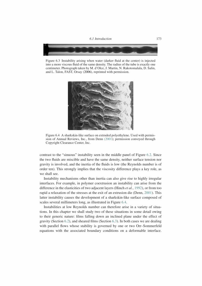
6.1 Introduction 173

Figure 6.3 Instability arising when water (darker fluid at the center) is injectedinto a more viscous fluid of the same density. The radius of the tube is exactly onecentimeter. Photograph taken by M. d’Olce, J. Martin, N. Rakotomalala, D. Salin,and L. Talon, FAST, Orsay (2006), reprinted with permission.

Figure 6.4 A sharkskin-like surface on extruded polyethylene. Used with permis-sion of Annual Reviews, Inc., from Denn (2001); permission conveyed throughCopyright Clearance Center, Inc.

contrast to the “sinuous” instability seen in the middle panel of Figure 6.2. Sincethe two fluids are miscible and have the same density, neither surface tension norgravity is involved, and the inertia of the fluids is low (the Reynolds number is oforder ten). This strongly implies that the viscosity difference plays a key role, aswe shall see.

Instability mechanisms other than inertia can also give rise to highly irregularinterfaces. For example, in polymer coextrusion an instability can arise from thedifference in the elasticities of two adjacent layers (Hinch et al., 1992), or from toorapid a relaxation of the stresses at the exit of an extrusion die (Denn, 2001). Thislatter instability causes the development of a sharkskin-like surface composed ofscales several millimeters long, as illustrated in Figure 6.4.

Instabilities at low Reynolds number can therefore arise in a variety of situa-tions. In this chapter we shall study two of these situations in some detail owingto their generic nature: films falling down an inclined plane under the effect ofgravity (Section 6.2), and sheared films (Section 6.3). In both cases we are dealingwith parallel flows whose stability is governed by one or two Orr–Sommerfeldequations with the associated boundary conditions on a deformable interface.

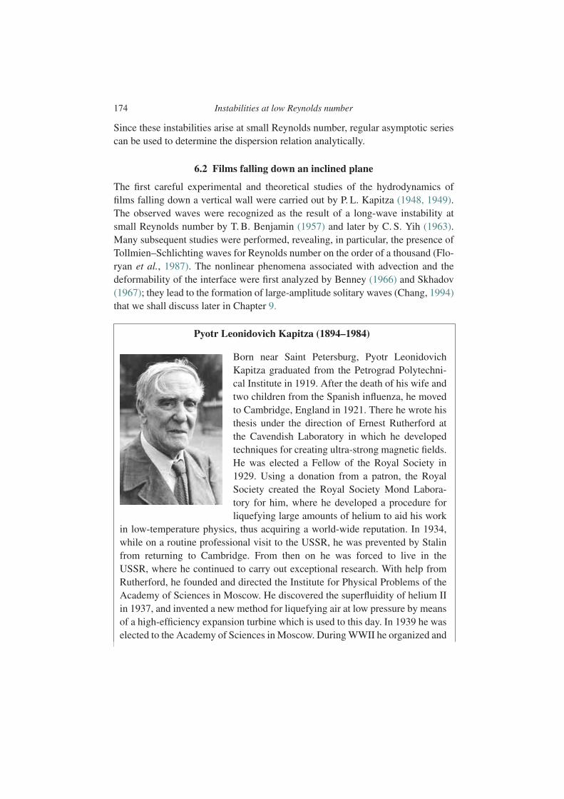
174 Instabilities at low Reynolds number

Since these instabilities arise at small Reynolds number, regular asymptotic seriescan be used to determine the dispersion relation analytically.

6.2 Films falling down an inclined plane

The first careful experimental and theoretical studies of the hydrodynamics offilms falling down a vertical wall were carried out by P. L. Kapitza (1948, 1949).The observed waves were recognized as the result of a long-wave instability atsmall Reynolds number by T. B. Benjamin (1957) and later by C. S. Yih (1963).Many subsequent studies were performed, revealing, in particular, the presence ofTollmien–Schlichting waves for Reynolds number on the order of a thousand (Flo-ryan et al., 1987). The nonlinear phenomena associated with advection and thedeformability of the interface were first analyzed by Benney (1966) and Skhadov(1967); they lead to the formation of large-amplitude solitary waves (Chang, 1994)that we shall discuss later in Chapter 9.

Pyotr Leonidovich Kapitza (1894–1984)

Born near Saint Petersburg, Pyotr LeonidovichKapitza graduated from the Petrograd Polytechni-cal Institute in 1919. After the death of his wife andtwo children from the Spanish influenza, he movedto Cambridge, England in 1921. There he wrote histhesis under the direction of Ernest Rutherford atthe Cavendish Laboratory in which he developedtechniques for creating ultra-strong magnetic fields.He was elected a Fellow of the Royal Society in1929. Using a donation from a patron, the RoyalSociety created the Royal Society Mond Labora-tory for him, where he developed a procedure forliquefying large amounts of helium to aid his work

in low-temperature physics, thus acquiring a world-wide reputation. In 1934,while on a routine professional visit to the USSR, he was prevented by Stalinfrom returning to Cambridge. From then on he was forced to live in theUSSR, where he continued to carry out exceptional research. With help fromRutherford, he founded and directed the Institute for Physical Problems of theAcademy of Sciences in Moscow. He discovered the superfluidity of helium IIin 1937, and invented a new method for liquefying air at low pressure by meansof a high-efficiency expansion turbine which is used to this day. In 1939 he waselected to the Academy of Sciences in Moscow. During WWII he organized and

6.2 Films falling down an inclined plane 175

directed the Department of Oxygen Industry affiliated with the government. In1945 he refused to work on nuclear weapons development under Beria, andconsequently was dismissed from his posts and sent to live in his house inthe countryside. There he worked on high-power electronics until the deathof Stalin and the arrest of Beria in 1953. In 1955 he returned to his positionas director of the Institute and continued his research on high-power electron-ics and plasmas. He was a great moral figure, brave and clever, and managedto free several colleagues from Stalin’s prisons, including Lev Landau, whohad been arrested by the NKVD on the pretext of spying. He later defendedAndrei Sakharov (A. Sakharov, Memoirs, Knopf, 1990). As a public figure hespoke out on various issues such as economics, ecology, and the organizationof science. He was awarded the Nobel Prize in Physics in 1978 for his work inlow-temperature physics.

6.2.1 Base flow and characteristic scales

We consider a film of incompressible liquid of thickness h, viscosity µ, and den-sity ρ, falling down a plane inclined at an angle θ with respect to the horizontal(Figure 6.5). The interface at the ambient gas of pressure P0 has surface tension γ .

The Navier–Stokes equations, subject to the boundary conditions of no-slip onthe lower surface and constant pressure P0 at the free surface, have a steady parallelflow solution corresponding to a planar interface and a parabolic velocity profile:

U (y)=U0(1− y2/h2), (6.1a)

V (y)=0, (6.1b)

P(y)− P0 =−ρgy cosθ, (6.1c)

where the velocity U0 of the interface is defined as

U0 = ρgh2 sinθ

2µ. (6.2)

This solution displays the natural scales of the problem: the thickness h of the film,the fluid density ρ, and the speed U0 of the fluid at the interface.

The importance of inertia relative to viscosity, gravity, and surface tension ismeasured respectively by the Reynolds, Froude, and Weber numbers, defined as

Re= ρU0h

µ, Fr= U 2

0

gh cosθ= Retanθ

2, We= ρU 2

0 h

γ. (6.3)

We note that the Froude number is defined using the gravity component g cosθnormal to the flow. To get an idea of the magnitudes of these parameters, for a slope

176 Instabilities at low Reynolds number

Figure 6.5 Film falling down an inclined plane showing the parabolic velocityprofile for a planar interface, and the perturbed interfacial position, η(x, t).

of θ =30 and a water film 0.1 mm thick, U0 =50 mm/s, and these three numbersare Re = 5, Fr = 1.4, and We = 0.003. For a film of oil of viscosity ten timeshigher and for the same film thickness and inclination angle, we have U0 =5 mm/s,Re=0.05, Fr=0.014, and We=0.00008.

When the interface is perturbed (η(x, t) =0 as in Figure 6.5), the velocity profileis no longer exactly parabolic. This, together with inertia, leads to the instabilitystudied below.

6.2.2 Formulation of the stability problem

Conservation equations and boundary conditions

Squire’s theorem, according to which the instability arises at the threshold for atwo-dimensional perturbation (Chapter 5), remains valid for a flow with an inter-face (Hesla et al., 1986). Therefore, for finding critical conditions it is sufficientto consider the planar problem defined by the two-dimensional Navier–Stokesequations in the longitudinal and transverse directions x and y, and by the bound-ary conditions at the wall and at the gas–liquid interface. Let us discuss theseboundary conditions. The conditions at the wall are the classic no-slip conditions:

U =0, V =0 at y =−h. (6.4)

At the interface there are two types of condition; kinematic ones reflecting theimpermeability of the interface, and dynamic ones on the stresses. These con-ditions, which are described in detail in Chapter 2 for the Rayleigh–Taylorinstability, involve the unit vectors normal and tangent to the interface, definedas

n= (−∂xη,1)√1+∂xη2

, t= (1,∂xη)√1+∂xη2

, (6.5)

where η(x, t) is the position of the interface.

6.2 Films falling down an inclined plane 177

• The kinematic condition is that the normal velocity U ·n of the fluid at the inter-face must be equal to the normal velocity of the interface w ·n=∂tη/

√1+∂xη2,

or

U (−∂xη)+V = ∂tη at y =η. (6.6)

• The dynamic conditions pertain to (i) the continuity of the tangential stress and(ii) the jump in the normal stress due to surface tension. Since the stress in thefluid is ·n, where is the stress tensor, and the effect of the air reduces to apurely normal stress −P0n, the dynamic condition is written as

t ·( ·n)=0 at y =η, (6.7a)

n ·( ·n)−n ·(−P0n)= γ

Rat y =η, (6.7b)

where R−1 =−divn= ∂xxη/(1+∂xη2)3/2 is the curvature of the interface.

For a Newtonian fluid these two equations become

−2µ∂xη

1+∂xη2(∂xU −∂y V )+µ

1−∂xη2

1+∂xη2(∂yU +∂x V )=0 at y =η, (6.8a)

−P + 2µ

1+∂xη2[∂xη

2∂xU +∂y V −∂xη(∂yU +∂x V )]+ P0 = γ

Rat y =η. (6.8b)

It can be verified that the base flow (6.1) is indeed a solution of the full Navier–Stokes equations with the boundary conditions (6.4), (6.7), and (6.8).

Perturbed flow, linearization, and normal modes

We choose the thickness h as the length scale and h/U0 as the time scale andintroduce the stream function ψ of the perturbations via1

U =U +∂yψ, V = V −∂xψ =−∂xψ. (6.9)

Eliminating the pressure from the Navier–Stokes equations by cross-differentiationand considering perturbations in the form of the normal modes

ψ(x, y, t)= ψ(y)eiα(x−ct), η(x, t)= ηeiα(x−ct), α= kh, (6.10)

the Navier–Stokes equations lead to the Orr–Sommerfeld equation (Chapter 5):

(D2 −α2)2ψ = iαRe[(U −c)(D2 −α2)− D2U

]ψ, (6.11)

1 This is how the problem was solved by Yih (1963); it is of course also possible to choose to retain the velocitiesand pressure as dependent variables (Smith, 1990).

178 Instabilities at low Reynolds number

where D is the derivative operator d/dy.The conditions (6.4) of no-slip on the wall become

Dψ(−1)=0, (6.12a)

ψ(−1)=0. (6.12b)

The kinematic condition at the interface (6.6) linearized about y =0 is written as

ψ(0)−(c−1)η=0. (6.13)

The dynamic condition (6.8b) at the interface involves the pressure, which can beeliminated in two steps by: (i) differentiating (6.8b) along the interface (∂P/∂s =∇ P ·t, where s is the curvilinear abscissa at the interface), and then (ii) eliminatingthe gradients ∂x P and ∂y P using the Navier–Stokes equations. The conditions(6.8) linearized about y =0 then become

D2ψ(0)+α2ψ(0)+ ηD2U (0)=0, (6.14a)

−D3ψ(0)+[3α2 − iαRe(c−1)

]Dψ(0)+ iαRe

(1

Fr+ α2

We

)η=0. (6.14b)

6.2.3 A long-wave interfacial instability

The Orr–Sommerfeld equation (6.11) together with the boundary conditions(6.12), (6.13), and (6.14) are a generalized eigenvalue problem with the speed cas the eigenvalue. We note that, in contrast to flow between rigid walls, the eigen-value appears not only in the equations but also in one of the boundary conditions,namely, Eq. (6.13) at the interface. Here we shall study the temporal stability ofthe base flow to a perturbation of real fixed wave number α and complex unknownspeed c. As usual, the real part cr corresponds to the wave speed (in units of U0),and σ =αci is the growth rate (in units of U0/h).

Asymptotic solution

Experiments show that on a film about a millimeter thick the instability is mani-fested as the growth of waves of wavelength on the order of several centimeters,which corresponds to a dimensionless wave number of α= kh ≈0.1. On the otherhand, since the Reynolds number is typically less than ten, inertial effects, whichaccording to the Orr–Sommerfeld equation (6.11) are of order αRe, are small.Finally, as we have seen, the Weber number is typically small as well. We thereforeconsider situations satisfying the following conditions:

α1, Re=O(1), We/α2 =O(1). (6.15)

6.2 Films falling down an inclined plane 179

For these long-wave perturbations the wave number α can be treated as a smallparameter, and the form of the equations suggests that the speed c and amplitudeψ of the eigenfunction can be sought as a series in powers of α as follows:

ψ(y)= ψ(0)(y)+αψ(1)(y)+ ..., (6.16a)

c = c(0)+αc(1)+ ... (6.16b)

Since we are solving a linear problem, where the solution can be determined onlyup to a multiplicative constant, the interface perturbation η can be treated as anormalization constant of the eigenfunctions, and there is no need to expand it ina series.

At lowest order the Orr–Sommerfeld equation reduces to

D4ψ(0)(y)=0, (6.17)

with boundary conditions at the wall (y =−1) and at the interface (y =0)

ψ(0)(−1)=0, (6.18a)

Dψ(0)(−1)=0, (6.18b)

D3ψ(0)(0)=0, (6.18c)

D2ψ(0)(0)−2ψ(0)(0)

c(0)−1=0. (6.18d)

Here we have used D2U (0)= −2, U0 =1, and have eliminated η. The solution ofthis Stokes (purely viscous) problem is written as

ψ(0)(y)= η(y +1)2, c(0) =2, (6.19)

where η is the amplitude of the deformation of the interface. The eigenvalue c(0)

is real and independent of the wave number, so that the perturbations all propagateat the same dimensional speed 2U0, independently of the wave number, that is,without dispersion. Since the imaginary part of c(0) is zero, the growth rate iszero and therefore there is no instability to the lowest order. In addition, since theratio of the amplitudes η and ψ(0) is real, the interface η and the stream functionψ are in phase. The velocity perturbations u = ∂yψ and v = −∂xψ are thereforerespectively in and out of phase with the interface, as illustrated in Figure 6.7bbelow. Therefore, at the lowest order the flow does not manifest any instability tolong-wavelength perturbations.

At first order the Orr–Sommerfeld equation becomes

D4ψ(1)(y)= iRe[(U −c(0))D2 − D2U

]ψ(0).

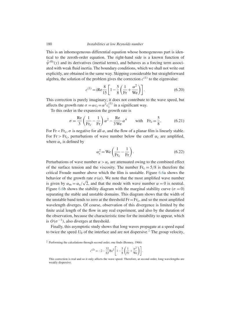
180 Instabilities at low Reynolds number

This is an inhomogeneous differential equation whose homogeneous part is iden-tical to the zeroth-order equation. The right-hand side is a known function ofψ(0)(y) and its derivatives (inertial terms), and behaves as a forcing term associ-ated with weak fluid inertia. The boundary conditions, which we shall not write outexplicitly, are obtained in the same way. Skipping considerable but straightforwardalgebra, the solution of the problem gives the correction c(1) to the eigenvalue:

c(1) = iRe8

15

[1− 5

8

(1

Fr+ α2

We

)]. (6.20)

This correction is purely imaginary; it does not contribute to the wave speed, butaffects the growth rate σ =αci =α2c(1)i in a significant way.

To this order in the expansion the growth rate is

σ = Re

3

(1

Frc− 1

Fr

)α2 − Re

3Weα4 with Frc = 5

8. (6.21)

For Fr<Frc, σ is negative for all α, and the flow of a planar film is linearly stable.For Fr > Frc, perturbations of wave number below the cutoff αc are amplified,where αc is defined by

α2c =We

(1

Frc− 1

Fr

). (6.22)

Perturbations of wave number α>αc are attenuated owing to the combined effectof the surface tension and the viscosity. The number Frc = 5/8 is therefore thecritical Froude number above which the film is unstable. Figure 6.6a shows thebehavior of the growth rate σ(α). We note that the most amplified wave numberis given by αm = αc/

√2, and that the mode with wave number α = 0 is neutral.

Figure 6.6b shows the stability diagram with the marginal stability curve (σ = 0)separating the stable and unstable domains. This diagram shows that the width ofthe unstable band tends to zero at the threshold Fr=Frc, and so the most amplifiedwavelength diverges. Of course, observation of this divergence is limited by thefinite axial length of the flow in any real experiment, and also by the duration ofthe observation, because the characteristic time for the instability to appear, whichis O(σ−1), also diverges at threshold.

Finally, this asymptotic study shows that long waves propagate at a speed equalto twice the speed U0 of the interface and are not dispersive.2 The group velocity,

2 Performing the calculations through second order, one finds (Benney, 1966)

c(2) =−2− 32

63Re2

[1− 5

8

(1

Fr+ α2

We

)].

This correction is real and so it only affects the wave speed. Therefore, at second order, long wavelengths areweakly dispersive.

6.2 Films falling down an inclined plane 181

(a)

Fr > Frc

Fr < Frc

(b)

Stable

Unstable

Fr

α

α

σ

Figure 6.6 (a) Behavior of the growth rate σ(α) for Fr < Frc and Fr > Frc; (b)stability diagram.

which is equal to the speed at the order we are considering, is therefore strictlypositive, which implies that the instability can only be convective. Beyond thecritical Froude number the destabilizing inertia dominates the stabilizing normalcomponent of gravity, and long waves are unstable. The growth rate is proportionalto the Reynolds number (σ ∝ α2Re), which demonstrates the inertial nature ofthe instability (the dimensional growth rate σU0/h is proportional to U 2

0 ). Thisinstability, where all wave numbers in the band 0 <α<αc are unstable, is calleda long-wave instability. Its mechanism is discussed in more detail in the followingsection.

The conclusions reached above are valid for long-wavelength perturbations forwhich α = kh 1. As far as short-wavelength perturbations are concerned, anasymptotic series for α 1 obtained by Yih (1963) shows that these waves arestable as a result of damping due to surface tension and viscous dissipation, asexpected.

Numerical solution

The problem defined by Eqs (6.11)–(6.14) with the restriction to long waves liftedcan be solved numerically. The Chebyshev polynomials Tj (y)= cos(n cos−1(y)),which were mentioned in Chapter 5, form a suitable basis on which to seek theamplitude of the unknown eigenfunction in the form

ψ(y)=n∑

j=0

a j Tj (y). (6.23)

Using recursion relations expressing the derivative of a polynomial as a linearcombination of other polynomials, the Orr–Sommerfeld equation and the boundaryconditions can then be used to transform the problem into an algebraic one wherethe unknowns are the coefficients a j . The number of polynomials necessary for the

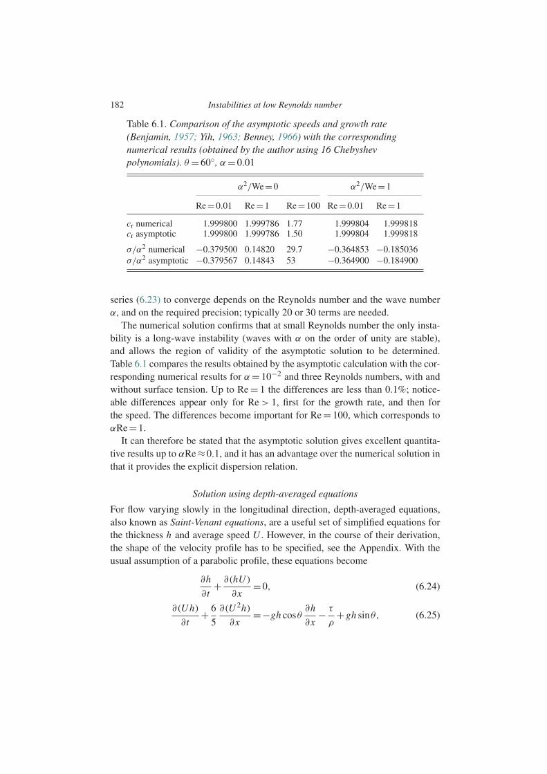
182 Instabilities at low Reynolds number

Table 6.1. Comparison of the asymptotic speeds and growth rate(Benjamin, 1957; Yih, 1963; Benney, 1966) with the correspondingnumerical results (obtained by the author using 16 Chebyshevpolynomials). θ =60, α=0.01

α2/We=0 α2/We=1

Re=0.01 Re=1 Re=100 Re=0.01 Re=1

cr numerical 1.999800 1.999786 1.77 1.999804 1.999818cr asymptotic 1.999800 1.999786 1.50 1.999804 1.999818

σ/α2 numerical −0.379500 0.14820 29.7 −0.364853 −0.185036σ/α2 asymptotic −0.379567 0.14843 53 −0.364900 −0.184900

series (6.23) to converge depends on the Reynolds number and the wave numberα, and on the required precision; typically 20 or 30 terms are needed.

The numerical solution confirms that at small Reynolds number the only insta-bility is a long-wave instability (waves with α on the order of unity are stable),and allows the region of validity of the asymptotic solution to be determined.Table 6.1 compares the results obtained by the asymptotic calculation with the cor-responding numerical results for α= 10−2 and three Reynolds numbers, with andwithout surface tension. Up to Re = 1 the differences are less than 0.1%; notice-able differences appear only for Re > 1, first for the growth rate, and then forthe speed. The differences become important for Re = 100, which corresponds toαRe=1.

It can therefore be stated that the asymptotic solution gives excellent quantita-tive results up to αRe≈0.1, and it has an advantage over the numerical solution inthat it provides the explicit dispersion relation.

Solution using depth-averaged equations

For flow varying slowly in the longitudinal direction, depth-averaged equations,also known as Saint-Venant equations, are a useful set of simplified equations forthe thickness h and average speed U . However, in the course of their derivation,the shape of the velocity profile has to be specified, see the Appendix. With theusual assumption of a parabolic profile, these equations become

∂h

∂t+ ∂(hU )

∂x=0, (6.24)

∂(Uh)

∂t+ 6

5

∂(U 2h)

∂x=−gh cosθ

∂h

∂x− τ

ρ+gh sinθ, (6.25)

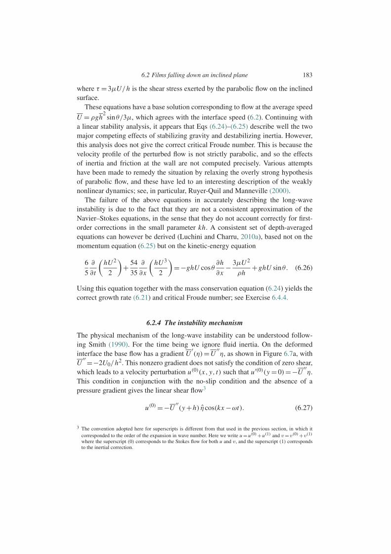
6.2 Films falling down an inclined plane 183

where τ =3µU/h is the shear stress exerted by the parabolic flow on the inclinedsurface.

These equations have a base solution corresponding to flow at the average speed

U = ρgh2

sinθ/3µ, which agrees with the interface speed (6.2). Continuing witha linear stability analysis, it appears that Eqs (6.24)–(6.25) describe well the twomajor competing effects of stabilizing gravity and destabilizing inertia. However,this analysis does not give the correct critical Froude number. This is because thevelocity profile of the perturbed flow is not strictly parabolic, and so the effectsof inertia and friction at the wall are not computed precisely. Various attemptshave been made to remedy the situation by relaxing the overly strong hypothesisof parabolic flow, and these have led to an interesting description of the weaklynonlinear dynamics; see, in particular, Ruyer-Quil and Manneville (2000).

The failure of the above equations in accurately describing the long-waveinstability is due to the fact that they are not a consistent approximation of theNavier–Stokes equations, in the sense that they do not account correctly for first-order corrections in the small parameter kh. A consistent set of depth-averagedequations can however be derived (Luchini and Charru, 2010a), based not on themomentum equation (6.25) but on the kinetic-energy equation

6

5

∂

∂t

(hU 2

2

)+ 54

35

∂

∂x

(hU 3

2

)=−ghU cosθ

∂h

∂x− 3µU 2

ρh+ghU sinθ. (6.26)

Using this equation together with the mass conservation equation (6.24) yields thecorrect growth rate (6.21) and critical Froude number; see Exercise 6.4.4.

6.2.4 The instability mechanism

The physical mechanism of the long-wave instability can be understood follow-ing Smith (1990). For the time being we ignore fluid inertia. On the deformedinterface the base flow has a gradient U

′(η)=U

′′η, as shown in Figure 6.7a, with

U′′ =−2U0/h2. This nonzero gradient does not satisfy the condition of zero shear,

which leads to a velocity perturbation u(0)(x, y, t) such that u′(0)(y =0)=−U′′η.

This condition in conjunction with the no-slip condition and the absence of apressure gradient gives the linear shear flow3

u(0) =−U′′(y +h) ηcos(kx −ωt). (6.27)

3 The convention adopted here for superscripts is different from that used in the previous section, in which itcorresponded to the order of the expansion in wave number. Here we write u =u(0)+u(1) and v=v(0)+v(1)

where the superscript (0) corresponds to the Stokes flow for both u and v, and the superscript (1) correspondsto the inertial correction.

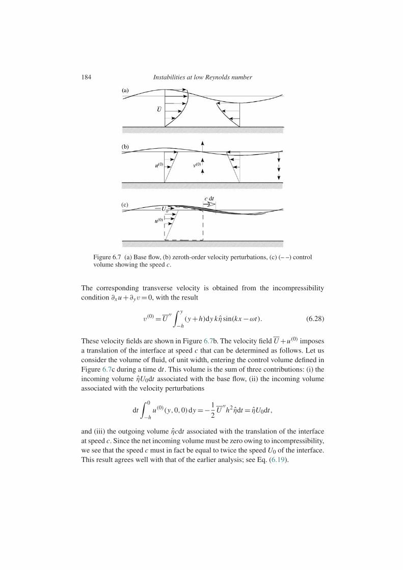
184 Instabilities at low Reynolds number

Figure 6.7 (a) Base flow, (b) zeroth-order velocity perturbations, (c) (– –) controlvolume showing the speed c.

The corresponding transverse velocity is obtained from the incompressibilitycondition ∂x u +∂yv=0, with the result

v(0) =U′′∫ y

−h(y +h)dy kη sin(kx −ωt). (6.28)

These velocity fields are shown in Figure 6.7b. The velocity field U +u(0) imposesa translation of the interface at speed c that can be determined as follows. Let usconsider the volume of fluid, of unit width, entering the control volume defined inFigure 6.7c during a time dt . This volume is the sum of three contributions: (i) theincoming volume ηU0dt associated with the base flow, (ii) the incoming volumeassociated with the velocity perturbations

dt∫ 0

−hu(0)(y,0,0)dy =−1

2U

′′h2ηdt = ηU0dt,

and (iii) the outgoing volume ηcdt associated with the translation of the interfaceat speed c. Since the net incoming volume must be zero owing to incompressibility,we see that the speed c must in fact be equal to twice the speed U0 of the interface.This result agrees well with that of the earlier analysis; see Eq. (6.19).

6.2 Films falling down an inclined plane 185

To exhibit and understand the instability it is necessary to calculate the inertialcorrection to the Stokes flow (6.27)–(6.28). This correction can be estimated usingdimensional arguments. In order to consider a stationary problem, we work in areference frame attached to the wave of speed c =2U0, so that the velocity profileof the base solution has the shape shown in Figure 6.8a. Two phenomena competeto first order: gravity, which has a stabilizing effect, and fluid inertia, which isdestabilizing. Let us first consider gravity (Figure 6.8b). The pressure p+ under apeak is higher than the pressure p− under a trough owing to the hydrostatic effect.This pressure difference gives rise to Poiseuille flow out of phase with the interfacedeformation, where the average speed u(1g) is such that

µu(1g)

h2∼ k(p+− p−)∼ρg cosθ kη (6.29)

or u(1g) ∼ kηU0. This flow drains the fluid from the peaks toward the troughs andtends to make the interface planar again; we note that this effect vanishes for avertical film. The second phenomenon, related to the inertia, is the sum of twocontributions: the advection of the perturbation u(0) by the base flow U − c, andthe advection of the transverse gradients U

′by the perturbation v(0). The first of

these two contributions, shown in Figure 6.8c, creates a flow u(1a) out of phasewith the interface such that

µu(1a)

h2∼ρU0ku(0) ∼ρ

U 20

hkη. (6.30)

The other contribution due to advection is expressed in the same way becauseρU0ku(0) ∼ ρv(0)U

′owing to the incompressibility. This inertial flow is directed

from the troughs to the peaks and therefore tends to amplify the perturbation.Each of the two flows, gravitational and inertial, produces a vertical velocityv(1) ∼ khu(1) in phase with the interface and contributes to the growth rate σ via aterm of the form

σ ∼ v(1)

η∼ kh

u(1)

η. (6.31)

When the inertial flow (6.30) is small compared to the gravitational flow (6.29), or

ρU 2

0

hkηρg cosθ kη, (6.32)

or equivalently Fr1, the stabilizing flow due to gravity dominates, and the planarfilm is stable. In the opposite case Fr1 the film is unstable. The marginal stabilitycondition corresponds to the two phenomena being in equilibrium, that is, Frc ∼1,and we obtain, up to a numerical factor of 5/8, the stability criterion in terms ofthe Froude number given by the exact calculation.

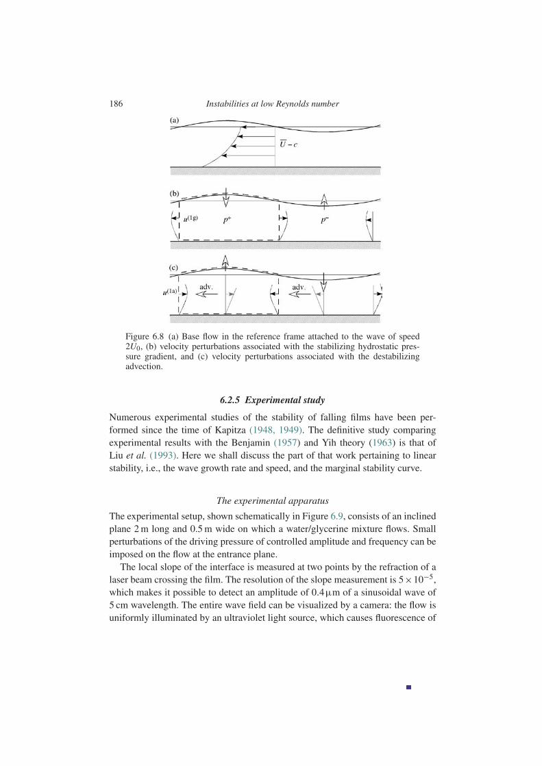
186 Instabilities at low Reynolds number

Figure 6.8 (a) Base flow in the reference frame attached to the wave of speed2U0, (b) velocity perturbations associated with the stabilizing hydrostatic pres-sure gradient, and (c) velocity perturbations associated with the destabilizingadvection.

6.2.5 Experimental study

Numerous experimental studies of the stability of falling films have been per-formed since the time of Kapitza (1948, 1949). The definitive study comparingexperimental results with the Benjamin (1957) and Yih theory (1963) is that ofLiu et al. (1993). Here we shall discuss the part of that work pertaining to linearstability, i.e., the wave growth rate and speed, and the marginal stability curve.

The experimental apparatus

The experimental setup, shown schematically in Figure 6.9, consists of an inclinedplane 2 m long and 0.5 m wide on which a water/glycerine mixture flows. Smallperturbations of the driving pressure of controlled amplitude and frequency can beimposed on the flow at the entrance plane.

The local slope of the interface is measured at two points by the refraction of alaser beam crossing the film. The resolution of the slope measurement is 5×10−5,which makes it possible to detect an amplitude of 0.4µm of a sinusoidal wave of5 cm wavelength. The entire wave field can be visualized by a camera: the flow isuniformly illuminated by an ultraviolet light source, which causes fluorescence of

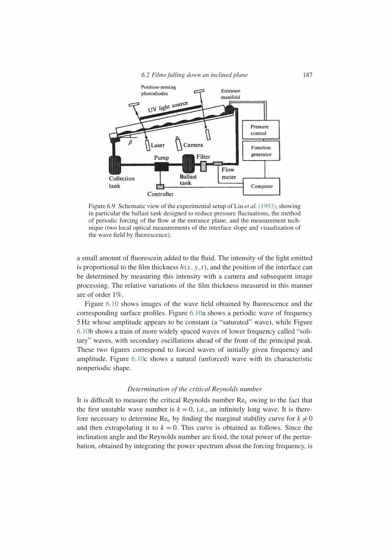
6.2 Films falling down an inclined plane 187

Figure 6.9 Schematic view of the experimental setup of Liu et al. (1993), showingin particular the ballast tank designed to reduce pressure fluctuations, the methodof periodic forcing of the flow at the entrance plane, and the measurement tech-nique (two local optical measurements of the interface slope and visualization ofthe wave field by fluorescence).

a small amount of fluorescein added to the fluid. The intensity of the light emittedis proportional to the film thickness h(x, y, t), and the position of the interface canbe determined by measuring this intensity with a camera and subsequent imageprocessing. The relative variations of the film thickness measured in this mannerare of order 1%.

Figure 6.10 shows images of the wave field obtained by fluorescence and thecorresponding surface profiles. Figure 6.10a shows a periodic wave of frequency5 Hz whose amplitude appears to be constant (a “saturated” wave), while Figure6.10b shows a train of more widely spaced waves of lower frequency called “soli-tary” waves, with secondary oscillations ahead of the front of the principal peak.These two figures correspond to forced waves of initially given frequency andamplitude. Figure 6.10c shows a natural (unforced) wave with its characteristicnonperiodic shape.

Determination of the critical Reynolds number

It is difficult to measure the critical Reynolds number Rec owing to the fact thatthe first unstable wave number is k = 0, i.e., an infinitely long wave. It is there-fore necessary to determine Rec by finding the marginal stability curve for k = 0and then extrapolating it to k = 0. This curve is obtained as follows. Since theinclination angle and the Reynolds number are fixed, the total power of the pertur-bation, obtained by integrating the power spectrum about the forcing frequency, is

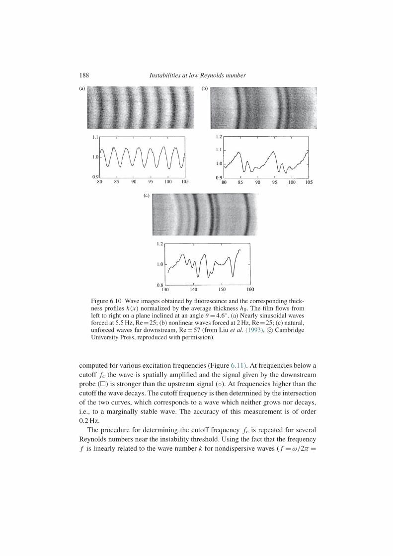
188 Instabilities at low Reynolds number

(a) (b)

(c)

Figure 6.10 Wave images obtained by fluorescence and the corresponding thick-ness profiles h(x) normalized by the average thickness h0. The film flows fromleft to right on a plane inclined at an angle θ = 4.6. (a) Nearly sinusoidal wavesforced at 5.5 Hz, Re=25; (b) nonlinear waves forced at 2 Hz, Re=25; (c) natural,unforced waves far downstream, Re = 57 (from Liu et al. (1993), c© CambridgeUniversity Press, reproduced with permission).

computed for various excitation frequencies (Figure 6.11). At frequencies below acutoff fc the wave is spatially amplified and the signal given by the downstreamprobe () is stronger than the upstream signal (). At frequencies higher than thecutoff the wave decays. The cutoff frequency is then determined by the intersectionof the two curves, which corresponds to a wave which neither grows nor decays,i.e., to a marginally stable wave. The accuracy of this measurement is of order0.2 Hz.

The procedure for determining the cutoff frequency fc is repeated for severalReynolds numbers near the instability threshold. Using the fact that the frequencyf is linearly related to the wave number k for nondispersive waves ( f =ω/2π =

6.2 Films falling down an inclined plane 189

Pow

er (

10–7

Hz–1

)

Forcing frequency (Hz)

Figure 6.11 Determination of the cutoff frequency fc from the strength of theslope signal as a function of the forcing frequency at the two abscissas x =43 cm() and x = 134 cm (), for θ = 5.6 and Re = 20.7 (from Liu et al. (1993), c©Cambridge University Press, reproduced with permission).

Re

f (H

z)

Figure 6.12 Marginal stability curves for θ = 5.6: (—) smoothed (Eq. (6.33))experimental points giving Rec = 12.4 ± 0.1, (- - -) asymptotic solution (6.21)giving Rec = 12.7, (...) approximate solution of Anshus and Goren (1966) (fromLiu et al. (1993), c© Cambridge University Press, reproduced with permission).

kc/2π ≈ kU0/π ) and taking into account (6.21) for the temporal growth rate, nearthe instability threshold we expect to find a relation of the type

fc ∼√

Re−Rec. (6.33)

(The control parameter chosen in this study is the Reynolds number, which isrelated to the Froude number as Fr= 1

2Re tanθ .) Then Rec is determined by finding

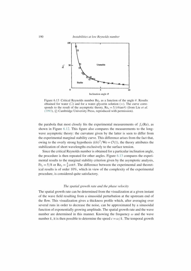
190 Instabilities at low Reynolds number

Inclination angle θ

Re c

Figure 6.13 Critical Reynolds number Rec as a function of the angle θ . Resultsobtained for water () and for a water–glycerin solution (×). The curve corre-sponds to the result of the asymptotic theory, Rec = 5/(4tanθ) (from Liu et al.(1993), c© Cambridge University Press, reproduced with permission).

the parabola that most closely fits the experimental measurements of fc(Re), asshown in Figure 6.12. This figure also compares the measurements to the long-wave asymptotic theory: the curvature given by the latter is seen to differ fromthe experimental marginal stability curve. This difference arises from the fact that,owing to the overly strong hypothesis (kh)2/We =O(1), the theory attributes thestabilization of short wavelengths exclusively to the surface tension.

Since the critical Reynolds number is obtained for a particular inclination angle,the procedure is then repeated for other angles. Figure 6.13 compares the experi-mental results to the marginal stability criterion given by the asymptotic analysis,Frc = 5/8 or Rec = 5

4 cotθ . The difference between the experimental and theoret-ical results is of order 10%, which in view of the complexity of the experimentalprocedure, is considered quite satisfactory.

The spatial growth rate and the phase velocity

The spatial growth rate can be determined from the visualization at a given instantof the wave field resulting from a sinusoidal perturbation at the upstream end ofthe flow. This visualization gives a thickness profile which, after averaging overseveral runs in order to decrease the noise, can be approximated by a sinusoidalfunction of exponentially growing amplitude. The spatial growth rate and the wavenumber are determined in this manner. Knowing the frequency ω and the wavenumber k, it is then possible to determine the speed c=ω/k. The temporal growth

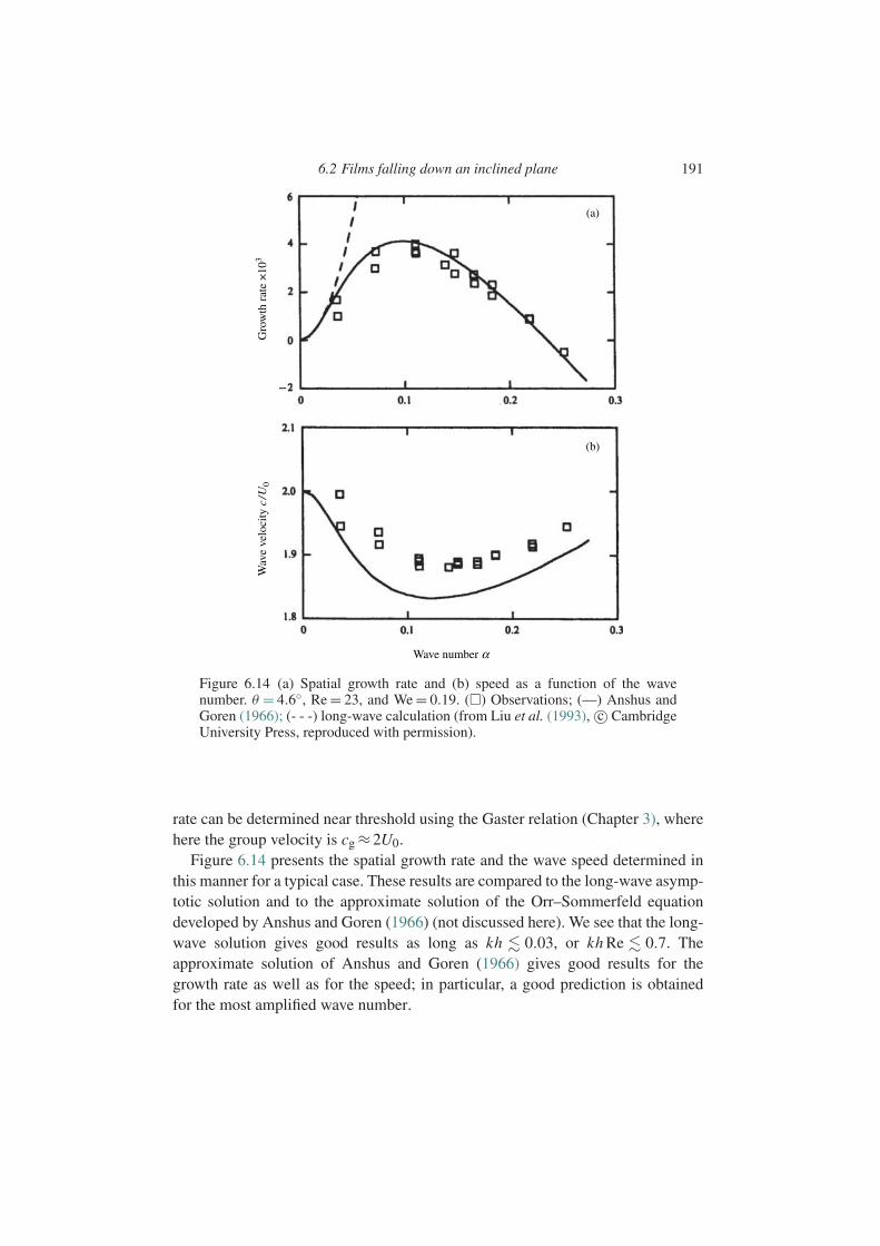
6.2 Films falling down an inclined plane 191

(a)

(b)

Wave number α

Gro

wth

rat

e ×

103

Wav

e ve

loci

ty c

/U0

Figure 6.14 (a) Spatial growth rate and (b) speed as a function of the wavenumber. θ = 4.6, Re = 23, and We = 0.19. () Observations; (—) Anshus andGoren (1966); (- - -) long-wave calculation (from Liu et al. (1993), c© CambridgeUniversity Press, reproduced with permission).

rate can be determined near threshold using the Gaster relation (Chapter 3), wherehere the group velocity is cg ≈2U0.

Figure 6.14 presents the spatial growth rate and the wave speed determined inthis manner for a typical case. These results are compared to the long-wave asymp-totic solution and to the approximate solution of the Orr–Sommerfeld equationdeveloped by Anshus and Goren (1966) (not discussed here). We see that the long-wave solution gives good results as long as kh 0.03, or kh Re 0.7. Theapproximate solution of Anshus and Goren (1966) gives good results for thegrowth rate as well as for the speed; in particular, a good prediction is obtainedfor the most amplified wave number.

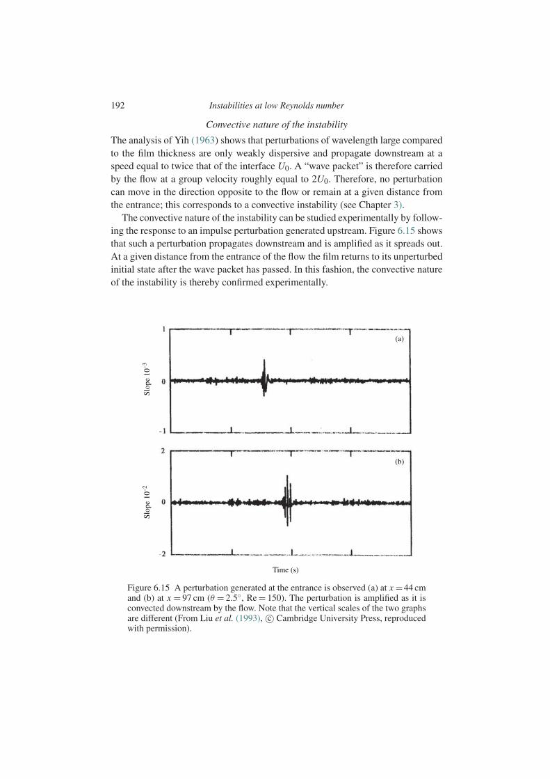
192 Instabilities at low Reynolds number

Convective nature of the instability

The analysis of Yih (1963) shows that perturbations of wavelength large comparedto the film thickness are only weakly dispersive and propagate downstream at aspeed equal to twice that of the interface U0. A “wave packet” is therefore carriedby the flow at a group velocity roughly equal to 2U0. Therefore, no perturbationcan move in the direction opposite to the flow or remain at a given distance fromthe entrance; this corresponds to a convective instability (see Chapter 3).

The convective nature of the instability can be studied experimentally by follow-ing the response to an impulse perturbation generated upstream. Figure 6.15 showsthat such a perturbation propagates downstream and is amplified as it spreads out.At a given distance from the entrance of the flow the film returns to its unperturbedinitial state after the wave packet has passed. In this fashion, the convective natureof the instability is thereby confirmed experimentally.

Slop

e 10

–3

(a)

(b)

Time (s)

Slop

e 10

–2

Figure 6.15 A perturbation generated at the entrance is observed (a) at x =44 cmand (b) at x = 97 cm (θ = 2.5, Re = 150). The perturbation is amplified as it isconvected downstream by the flow. Note that the vertical scales of the two graphsare different (From Liu et al. (1993), c© Cambridge University Press, reproducedwith permission).

6.3 Sheared liquid films 193

6.2.6 Instability of the wall mode at small slope

For a small slope θ , the critical Reynolds number Rec = 54 cotθ of the interfacial

mode becomes very large. An instability is then manifested which is associatedwith the growth of Tollmien–Schlichting waves near the wall, via a mechanismidentical to that of the boundary-layer instability or Poiseuille flow. This instability,which has been calculated by Floryan et al. (1987), is characterized by the fact thatthe maximum of the eigenfunctions is localized near the wall, and no longer nearthe interface as for the interfacial mode. This instability makes the flow evolverapidly toward turbulence.

6.3 Sheared liquid films

6.3.1 Introduction

Several of the physical situations listed in the introduction to this chapter involvetwo or more superposed fluid layers produced by a pressure gradient (Poiseuilleflow) or by a shear (Couette flow). Analysis of the stability of this type of flow leadsto an Orr–Sommerfeld equation for each layer, coupled by four conditions on thevelocities and the stresses at the interfaces. A good introduction to the problem ofa liquid film sheared by a (turbulent) air flow is provided by the review of Hanratty(1983). In the simplest case of the viscous flow of two liquids, the stability tolong-wavelength perturbations, i.e., perturbations with kh 1, has been solved byYih (1967). Short-wavelength perturbations have been considered by Hooper andBoyd (1983) and Hinch (1984), and Tollmien–Schlichting waves by Hooper andBoyd (1987). Situations not amenable to solution by asymptotic series, typicallywhere kh ∼ 1 and Re ≥ 1, have been analyzed numerically (Renardy, 1985). Thestudy of annular flows, begun by Hickox (1971), has been reviewed by Josephet al. (1997).

The analysis of Yih (1967) reveals a simple criterion for instability to long-wavelength perturbations: it is sufficient that the thinnest layer is the most viscousone. Here we shall describe the mechanism of this instability and obtain this resultby dimensional arguments (Charru and Hinch, 2000).

We consider a film of thickness h1 sufficiently thin compared to the characteris-tic thickness h2 of the other fluid, so that the flow near the film can be considereda planar shear flow, as shown in Figure 6.16a. In the case of Couette flow or for asolid wall which imposes a speed U0 on fluid 2 of thickness h2, the unperturbedflow is given exactly by

U 1 =UIy

h1, U 2 =UI +(U0 −UI)

y −h1

h2, (6.34)

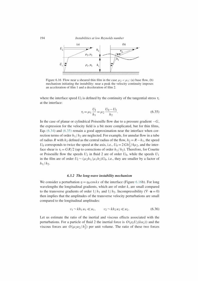
194 Instabilities at low Reynolds number

Figure 6.16 Flow near a sheared thin film in the case µ2 <µ1: (a) base flow, (b)mechanism initiating the instability: near a peak the velocity continuity imposesan acceleration of film 1 and a deceleration of film 2.

where the interface speed UI is defined by the continuity of the tangential stress τi

at the interface:

τi =µ1UI

h1=µ2

U0 −UI

h2. (6.35)

In the case of planar or cylindrical Poiseuille flow due to a pressure gradient −G,the expression for the velocity field is a bit more complicated, but for thin films,Eqs (6.34) and (6.35) remain a good approximation near the interface when cor-rection terms of order h1/h2 are neglected. For example, for annular flow in a tubeof radius R with h2 defined as the central radius of the flow, h2 = R−h1, the speedU0 corresponds to twice the speed at the axis, i.e., U0 =2 Gh2

2/4µ2, and the inter-face shear is τi = G R/2 (up to corrections of order h1/h2). Therefore, for Couetteor Poiseuille flow the speeds U2 in fluid 2 are of order U0, while the speeds U1

in the film are of order UI ∼ (µ2h1/µ1h2)U0, i.e., they are smaller by a factor ofh1/h2.

6.3.2 The long-wave instability mechanism

We consider a perturbation η= η0 coskx of the interface (Figure 6.16b). For longwavelengths the longitudinal gradients, which are of order k, are small comparedto the transverse gradients of order 1/h1 and 1/h2. Incompressibility (∇ ·u = 0)then implies that the amplitudes of the transverse velocity perturbations are smallcompared to the longitudinal amplitudes:

v1 ∼ kh1 u1 u1, v2 ∼ kh2 u2 u2. (6.36)

Let us estimate the ratio of the inertial and viscous effects associated with theperturbations. For a particle of fluid 2 the inertial force is O(ρ2U2(ku2)) and theviscous forces are O(µ2u2/h2

2) per unit volume. The ratio of these two forces

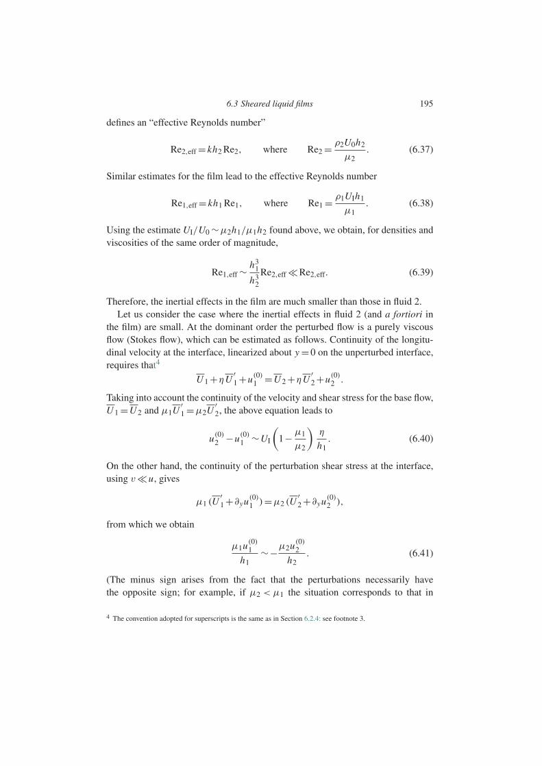
6.3 Sheared liquid films 195

defines an “effective Reynolds number”

Re2,eff = kh2 Re2, where Re2 = ρ2U0h2

µ2. (6.37)

Similar estimates for the film lead to the effective Reynolds number

Re1,eff = kh1 Re1, where Re1 = ρ1UIh1

µ1. (6.38)

Using the estimate UI/U0 ∼µ2h1/µ1h2 found above, we obtain, for densities andviscosities of the same order of magnitude,

Re1,eff ∼h3

1

h32

Re2,eff Re2,eff. (6.39)

Therefore, the inertial effects in the film are much smaller than those in fluid 2.Let us consider the case where the inertial effects in fluid 2 (and a fortiori in

the film) are small. At the dominant order the perturbed flow is a purely viscousflow (Stokes flow), which can be estimated as follows. Continuity of the longitu-dinal velocity at the interface, linearized about y =0 on the unperturbed interface,requires that4

U 1 +ηU′1 +u(0)

1 =U 2 +ηU′2 +u(0)

2 .

Taking into account the continuity of the velocity and shear stress for the base flow,U 1 =U 2 and µ1U

′1 =µ2U

′2, the above equation leads to

u(0)2 −u(0)

1 ∼UI

(1− µ1

µ2

)η

h1. (6.40)

On the other hand, the continuity of the perturbation shear stress at the interface,using vu, gives

µ1 (U′1 +∂yu(0)

1 )=µ2 (U′2 +∂yu(0)

2 ),

from which we obtain

µ1u(0)1

h1∼−µ2u(0)

2

h2. (6.41)

(The minus sign arises from the fact that the perturbations necessarily havethe opposite sign; for example, if µ2 < µ1 the situation corresponds to that in

4 The convention adopted for superscripts is the same as in Section 6.2.4: see footnote 3.

196 Instabilities at low Reynolds number

Figure 6.16, where the film is accelerated (u(0)1 > 0) and fluid 2 is decelerated

(u(0)2 <0).) Combining (6.40) and (6.41) we obtain the velocity perturbations:

u(0)1 ∼ η

h2

µ1 −µ2

µ2UI, u(0)

2 ∼−µ1h2

µ2h1u(0)

1 . (6.42)

Using the approximation of Stokes flow, these velocity perturbations, shownin Figure 6.17a, are therefore in phase with the deformation η of the interface.From the kinematic condition ∂tη= v

(0)1 −UI∂xη at the interface we find that the

perturbations propagate without growing or decaying at the speed

c ∼UI. (6.43)

In order to obtain an instability it is necessary, as for the falling film studiedin the preceding section, to include weak inertial corrections to the Stokes flow(6.42). Since according to (6.39) the inertial effects in the film are negligible, onlythe inertia of fluid 2 needs to be taken into account. We present the argumentin terms of vorticity perturbations ω2, the transport equation for which does not

Figure 6.17 Longitudinal velocity perturbations induced by a sinusoidal defor-mation η(x) of the bed and the associated vorticity: (a) Stokes flow in phase withη(x), (b) out-of-phase inertial correction.

6.3 Sheared liquid films 197

involve the pressure and is written as

ρ2dω2

dt=µ2ω2. (6.44)

For long-wave perturbations (kh2 1), to leading order this equation reduces toω

(0)2 = 0 corresponding to the Stokes flow estimated above and shown in Figure

6.17a. At the next order the inertial correction ω(1)2 is found from dimensional

arguments to be

µ2ω

(1)2

h22

∼ρ2kU0ω(0)2 ,

or ω(1)2 ∼ kh2Re2ω

(0)2 . This correction due to advection is out of phase with ω

(0)2 ,

as illustrated in Figure 6.17b (the π/2 phase lag can be derived by studying theequation for the complex amplitude ω

(1)2 of a normal mode, which involves a factor

ik coming from the derivative with respect to x in the advective term). The vorticityω

(1)2 gives rise to a longitudinal flow of order u(1)

2 ∼ω(1)2 h2, which at the interface

must match the flow in the film. Therefore, u(1)2 must vanish at the interface, and

so the correction u(1)2 must have the form shown in Figure 6.17b. This correction

gives rise to a shearing τ(1)i ∼µ2ω

(1)2 of the film, which then responds with a flow

satisfying µ1u(1)1 /h1 ∼ τ

(1)i . Putting all these estimates together, we find

u(1)1 ∼ kh2Re2

µ1 −µ2

µ2

η

h2UI, with UI ∼ µ2h1

µ1h2U0. (6.45)

For µ2 < µ1 the flow is directed from the troughs to the peaks, and thereforeamplifies the initial perturbation. We then obtain the growth rate σ ∼ v

(1)1 /η ∼

kh1u(1)1 η, or

σ ∼ (kh1)2Re2

µ1 −µ2

µ1

U0

h2. (6.46)

Therefore, by dimensional analysis we have recovered the major results ofthe complete stability analysis, i.e., (i) when fluid 1 is less viscous than fluid 2,the growth rate is negative and so the flow is stable, while in the opposite case theflow is unstable, and (ii) the mechanism involves both weak inertia and viscositystratification.

6.3.3 Waves of shorter wavelength

The above dimensional analysis is valid as long as the transverse gradients in fluid2 are of order 1/h2, a hypothesis which is always true for waves of sufficiently long

198 Instabilities at low Reynolds number

wavelength, but which may not hold for waves of shorter wavelength. By “wavesof shorter wavelength” we mean waves for which the penetration depth δ of thevorticity perturbations governed by (6.44) becomes smaller than the transversescale h2. The relevant transverse scale is then no longer h2 but rather δ. This depthδ is obtained by taking the inertial and viscous effects to be of the same order ofmagnitude:5

ρ2kU0ω2 ∼µ2ω2

δ2, (6.47)

where U0 ∼ (τi/µ2)δ is the speed at a distance δ from the interface. We then find

δ=(

kµ22

ρ2τi

)1/3

. (6.48)

Repeating the analysis of the perturbed flow taking δ as the characteristic trans-verse scale, we find that the growth rate no longer varies as (kh1)

2 but rather as(kh1)

4/3; however, the prefactor is always proportional to the difference (µ1 −µ2)(Charru and Hinch, 2000).

The qualitative result obtained for long wavelengths (kh2 1) therefore remainsvalid for smaller wavelengths (kδ 1): a thin film is unstable if it is sheared by aless viscous fluid, and stable in the opposite case. As mentioned in the introductionto this chapter, this property is used by the oil industry to transport very viscousoils, where a water film is injected at the wall of the pipe (Figure 6.2).

6.3.4 Instability of a falling film revisited

We end this chapter with a comparison of the instabilities of a falling film anda sheared film. The analyses in both cases display on the one hand an initiationmechanism, and on the other an amplification mechanism. For the falling film theinitiation mechanism resides in the continuity of the shear at the free surface, whilefor the sheared film it resides in the continuity of the velocity at the interface. Theseinitiation mechanisms cause the development of purely viscous perturbations. Inboth cases it is then advection due to weak inertia that is responsible for amplifyingthe perturbations, directly for the falling film and in a more indirect manner via theinterface stress τ

(1)i for the sheared film.

5 Beyond δ the perturbations tend to zero in an irrotational layer of thickness k−1. This potential layercorresponds to the “upper deck” of the triple-deck theory (Cousteix and Mauss, 2006).

6.4 Exercises 199

6.4 Exercises

6.4.1 Critical slope for a falling film

1. Derive the relations (6.1) defining the base flow. Find the thickness of a waterfilm (µ=10−3 Pa s) on a 1-m wide plane inclined at 10 for a flow rate of 1 l/minper meter of cross-section. What is this thickness for a film of oil of viscosityeight times higher, keeping the flow rate fixed? How does this thickness changewhen the slope is increased?

2. Determine the critical slope beyond which a water film becomes unstable, for aflow rate of 1 l/min per meter of width.

6.4.2 Boundary conditions on a free interface

1. Rederive the expression for the kinematic condition (6.6) using the principleof mass conservation in a control volume of thickness dx and bounded by thelower wall and the interface.

2. Derive the linearized boundary conditions (6.13)–(6.14). Start by finding thetwo conditions (6.8) on the interface stresses, and then linearizing them. It isimportant, in particular, to carefully linearize the pressure at the interface usinga Taylor series approach:

P(η)= P(η)+ p(η)= P(0)+η∂y P(0)+ p(0)+O(η2).

6.4.3 Solution for long waves

1. Derive the system of Stokes equations (6.17)–(6.18) starting from (6.11)–(6.13). Solve this system and obtain the solution (6.19).

2. Carry out the algebra required to calculate the inertial correction and find thegrowth rate σ =αci, where ci is given by (6.20).

6.4.4 Stability using the depth-averaged equations

Consider the consistent depth-averaged equations (6.24) and (6.26) for the fallingfilm.

1. Show that these equations admit a base flow solution h and U for the filmthickness and mean velocity, given by

U = ρgh2

sinθ

3µ, Q =U h,

where Q is the imposed flow rate per unit width.

200 Instabilities at low Reynolds number

2. Taking h and h/U as the length and time scales, show that the linearized massand kinetic-energy equations for the dimensionless disturbances η and u are

∂tη+∂xη+∂x u = 0,

3

5∂tη+ 6

5∂t u + 27

35∂xη+ 81

35∂x u = −∂xη

Fr+ 3

Re(2η−u) ,

where Re=ρUh/µ and Fr=U2/gh.

3. Introducing disturbances proportional to eiα(x−ct), show that the dispersionrelation is

6

5c2 − 102

35c+ 54

35= 1

Fr+ 3

iαRe(c−3).

4. For αRe small (as it must be here), expand the eigenvalue as c = c(0)+αRec(1)

and show that one of the two roots is given by

c(0) =3, c(1) = i

3(Fr

−1c −Fr

−1),

where Frc = 5/18 is the critical Froude number. Verify that this result corre-sponds to the same dimensional wave velocity and growth rate as those obtainedfrom the Orr–Sommerfeld equations (i.e., c = c(0) +αc(1), where c(0) and c(1)

are given by (6.19) and (6.20) with the interface velocity U0 = 32U as the

velocity scale).5. Show that the other root of the dispersion relation corresponds to a strongly

damped mode.

7

Avalanches, ripples, and dunes

7.1 Introduction

In this chapter we present an introduction to dense granular flows and their sta-bility by discussing two classes of phenomena: avalanches on an inclined plane,and particle transport on an erodible bed sheared by a fluid flow. These granularflows lead to the appearance of surface waves, called ripples or dunes dependingon whether their wavelength is of a few centimeters or a few meters (the relevanceof this common distinction will be discussed later on). Owing to the difficulty –both experimental and theoretical – of studying granular media, the mechanismsresponsible for these waves remain poorly understood, and so the results presentedin this chapter are definitely less well established than those in the precedingchapters.

Avalanches, ripples, and dunes present serious problems for human activities.Among natural phenomena, snow and mud avalanches are well known for theirdestructive nature; the displacement of a sand dune by the wind – the so-calledaeolian dunes – while less dramatic, can cut communication links and threatenhabitation and industrial installations. Subaqueous dunes perturb navigation inrivers and shallow seas such as the North Sea, while on river bottoms such dunesincrease friction and raise the water level, thereby contributing to flooding. Granu-lar flows are also omnipresent in industry: flow and transport of coal, constructionmaterials (cement, sand, gravel), agricultural foodstuffs, pharmaceutical materials,and sand from oilfields are some examples. Instabilities occur in the conduits usedto transport these materials, giving rise to dunes which perturb the flow and mayform obstructions, causing serious damage to operating equipment.

When studying the situations mentioned above, the first problem to consider,before dealing with instabilities, is how to model a granular flow. This requiresunderstanding the relation between the stresses and deformations of the granu-lar medium. Depending on how it is prepared, a noncohesive granular medium

201

202 Avalanches, ripples, and dunes

may behave like an elastic solid (for example, scree), or it may undergo plasticdeformation (sand underfoot), or it may flow like a fluid (sand in an hour glass).The general behavior of a granular medium therefore admits no simple descrip-tion, and so it is much more difficult to study than an elastic solid or a Newtonianfluid.1 This is because, first of all, there is not a large separation between the scaleof the observed phenomena (on the order of a meter or less) and the grain size (onthe order of a millimeter or more), with the result that finite-size effects play a roleand fluctuations remain important. Second, the interaction between the grains iscomplicated, much more so than that between molecules. It is dissipative owing tofriction between grains, and it involves the grain shape and the packing geometry.This leads to both strongly nonlinear and threshold behavior, which can dependon the history of the medium. Therefore, there is no general statistical mechanicstheory available for granular media, in contrast to simpler materials. A further dif-ficulty is the interaction of the grains with the interstitial fluid, either a gas or aliquid: when this interaction is negligible, the granular medium is termed “dry.”

It was Coulomb who, at the end of the 18th century, first developed a model of adry granular medium, introducing a relation of proportionality between the normaland tangential stresses at contact involving a friction coefficient. This simple lawsucceeds remarkably well in describing a number of static phenomena, but it failsto describe flows, at least in its elementary version where the friction coefficientis constant. Improvement of this law using the physics of granular media is atpresent the object of very active numerical, experimental, and theoretical research.The prospects of obtaining a general theory remain rather remote, but some realprogress has been made (Aranson and Tsimring, 2006).

The following section is devoted to surface waves and avalanches. The thirdsection deals with the modeling of granular transport on a bed sheared by aflow, including some recent concepts regarding relaxation phenomena. This is fol-lowed by a quick overview of aeolian and subaqueous ripples and dunes, from theviewpoint of dimensional analysis (Section 7.4). We then give a more detailed dis-cussion of the formation of subaqueous ripples in continuous flow (Section 7.5)and in oscillating flow (Section 7.6). Finally, we conclude this chapter with ananalysis of the formation of subaqueous dunes (Section 7.7).

7.2 Avalanches

When the slope of a granular pile exceeds a critical value of about 30, the surfaceof the granular medium suddenly begins to move (GDR MiDi, 2004; Forterre and

1 Cohesive effects of electrostatic or capillary origin, which are manifested for tiny grains typically smaller than10 µm, will not be considered in this chapter.

7.2 Avalanches 203

Figure 7.1 View from above of surface waves on a sand flow (grain diameterd =0.8 mm, slope α=34, thickness h=4.6 mm, flow width W =70 cm) (Forterreand Pouliquen, 2003).

Pouliquen, 2008). This avalanche phenomenon can also arise following a physicalmodification of the medium, for example, a change in the grain cohesion (as insnow avalanches) or the interstitial water content (as in landslides).

Here we shall consider the special case of a granular flow on a rough inclinedplane, where the thickness h is of a few tens of grain diameters. Surface wavesappear, as shown in Figure 7.1. These waves have a triangular profile, a wave-length long compared to the thickness h, and an amplitude of order h. As shownby Forterre and Pouliquen (2003), whose work we report here, these waves corre-spond to an inertial instability very similar to the instability of a liquid film studiedin the preceding chapter.

7.2.1 Particle flow on a rough inclined plane

The Saint-Venant equations

We consider a granular flow on a rough plane inclined at an angle α to the hori-zontal.2 When the scale on which the flow varies in the longitudinal direction x islarge compared to the layer thickness, a good description of the flow is given by the

2 Here we use α rather than θ to denote this angle, reserving θ for the Shields number, to be consistent with theliterature on granular media.

204 Avalanches, ripples, and dunes

mass and momentum conservation equations integrated over the thickness of thelayer, with some simplifying assumptions. These Saint-Venant equations, derivedin the Appendix, govern the evolution of the depth-averaged speed U (x, t) and thethickness h(x, t). For plug flow (i.e., flow with uniform velocity in the directionnormal to the plane), these equations become

∂t h +∂x (hU )=0, (7.1a)

ρh ∂tU +ρhU ∂xU =−ρgh cosα∂x h −τ +ρgh sinα, (7.1b)

where ρ is the density of the dense flow, which we assume to be uniform, andτ is the shear stress exerted by the bed on the flowing material. The rheology ofthe medium is not involved in the conservation equations (7.1), but it does enterinto the modeling of the stress τ . This modeling is crucial because it governs theessentials of the stability properties. Inspired by the Coulomb laws for dry frictionbetween two solids, we assume that this stress is proportional to the hydrostaticpressure, i.e.,

τ =µf ρgh cosα, (7.2)

where µf is a friction coefficient. The expression for this coefficient as a functionof U and h, or, rather, as a function of the dimensionless parameters of the problemin the form of a constitutive law, corresponds to the desired modeling. Once theconstitutive law is chosen, the Saint-Venant equations admit a base solution U andh defined by the two equations

µf(U ,h)= tanα, Q =U h, (7.3)

where Q is the imposed flow rate per unit width. We note that the significanceof the first of the above equations is that the values of U and h are such that thefriction coefficient is exactly tanα.

Constitutive laws for the friction coefficient

The easiest approach would be to choose the friction coefficient µf to be a constant,but this is not satisfactory. In fact, a constant friction coefficient would imply theexistence of only a single slope α = tan−1 µf at which a stationary and uniformflow would be possible. However, experiments (see for example Pouliquen (1999))show that such a flow exists for a range of slopes of several degrees about a typicalvalue of 30. Pouliquen (1999) therefore proposed a more elaborate constitutivelaw involving an important length scale: the residual thickness of the granular layerat which the grains stop moving when the upstream supply of material is cut off.This scale, denoted hstop, is characteristic of the type of grain and decreases with

7.2 Avalanches 205

the slope α, as shown later in Figure 7.4. The relation between the speed andthickness of the granular layer is then well represented by an expression of the form

U√gh

= c1h

hstop(α), µ f (U,h)= tanα, (7.4)

where c1 is a coefficient whose value depends on the type of grain. The above tworelations, together with an empirical rule hstop(α), completely define a relationbetween U and h in terms of the parameter α and therefore, together with therelation Q =Uh, completely define the base solution.

We note that the case of an avalanche on an erodible bed, a typical exampleof which is a sand avalanche on the surface of a dune or a simple pile, can bedescribed using Saint-Venant equations of the same type, by introducing an addi-tional term describing grain exchange between the immobile substrate and thelayer of mobile particles (Aradian et al., 2002).

7.2.2 Linear stability

Linearizing the full nonlinear equations (7.1) about the base solution defined by(7.3) with the constitutive law (7.4) results in a set of equations governing smallperturbations. Introducing normal modes proportional to eik(x−ct) in the usual wayand after some straightforward algebra, we find the dispersion relation

(c/U −1)2 + ia

kh Fr(c/U −1)− 1

Fr

(1− ib

kh

)=0, (7.5)

where Fr = U2/(gh cosα) is the Froude number of the base flow and a and b

are two coefficients coming from the perturbation of the constitutive law (7.4)defined as

a =U∂µf

∂U, b = h

∂µf

∂h. (7.6)

Experiments show that the coefficient a is positive while b is negative, i.e., thefriction coefficient increases with U and decreases with h.

For a given wave number k the dispersion relation (7.5) possesses two rootsc±. We note first of all that for constant friction coefficient the coefficients a andb vanish, and there is no instability. In this case, neutral perturbations propagatewith speed

c± =U ±√

gh cosα (7.7)

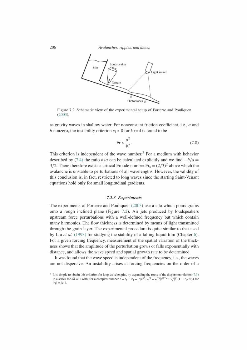
206 Avalanches, ripples, and dunes

Figure 7.2 Schematic view of the experimental setup of Forterre and Pouliquen(2003).

as gravity waves in shallow water. For nonconstant friction coefficient, i.e., a andb nonzero, the instability criterion ci >0 for k real is found to be

Fr>a2

b2. (7.8)

This criterion is independent of the wave number.3 For a medium with behaviordescribed by (7.4) the ratio b/a can be calculated explicitly and we find −b/a =3/2. There therefore exists a critical Froude number Frc = (2/3)2 above which theavalanche is unstable to perturbations of all wavelengths. However, the validity ofthis conclusion is, in fact, restricted to long waves since the starting Saint-Venantequations hold only for small longitudinal gradients.

7.2.3 Experiments

The experiments of Forterre and Pouliquen (2003) use a silo which pours grainsonto a rough inclined plane (Figure 7.2). Air jets produced by loudspeakersupstream force perturbations with a well-defined frequency but which containmany harmonics. The flow thickness is determined by means of light transmittedthrough the grain layer. The experimental procedure is quite similar to that usedby Liu et al. (1993) for studying the stability of a falling liquid film (Chapter 6).For a given forcing frequency, measurement of the spatial variation of the thick-ness shows that the amplitude of the perturbation grows or falls exponentially withdistance, and allows the wave speed and spatial growth rate to be determined.

It was found that the wave speed is independent of the frequency, i.e., the wavesare not dispersive. An instability arises at forcing frequencies on the order of a

3 It is simple to obtain this criterion for long wavelengths, by expanding the roots of the dispersion relation (7.5)in a series for kh 1 with, for a complex number z = zr + izi =|z|eiθ ,

√z =√|z|eiθ/2 ∼√|z|(1+ izi/2zr) for

|zi| |zr|.

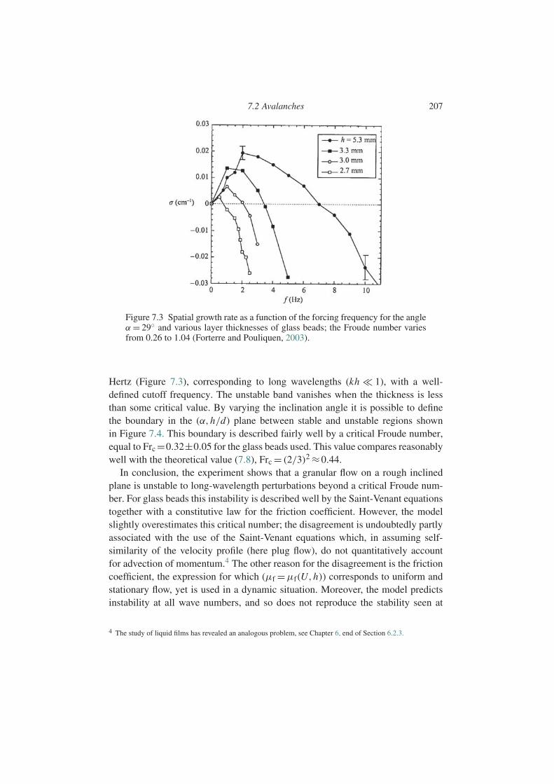
7.2 Avalanches 207

Figure 7.3 Spatial growth rate as a function of the forcing frequency for the angleα = 29 and various layer thicknesses of glass beads; the Froude number variesfrom 0.26 to 1.04 (Forterre and Pouliquen, 2003).

Hertz (Figure 7.3), corresponding to long wavelengths (kh 1), with a well-defined cutoff frequency. The unstable band vanishes when the thickness is lessthan some critical value. By varying the inclination angle it is possible to definethe boundary in the (α,h/d) plane between stable and unstable regions shownin Figure 7.4. This boundary is described fairly well by a critical Froude number,equal to Frc =0.32±0.05 for the glass beads used. This value compares reasonablywell with the theoretical value (7.8), Frc = (2/3)2 ≈0.44.

In conclusion, the experiment shows that a granular flow on a rough inclinedplane is unstable to long-wavelength perturbations beyond a critical Froude num-ber. For glass beads this instability is described well by the Saint-Venant equationstogether with a constitutive law for the friction coefficient. However, the modelslightly overestimates this critical number; the disagreement is undoubtedly partlyassociated with the use of the Saint-Venant equations which, in assuming self-similarity of the velocity profile (here plug flow), do not quantitatively accountfor advection of momentum.4 The other reason for the disagreement is the frictioncoefficient, the expression for which (µf =µf(U,h)) corresponds to uniform andstationary flow, yet is used in a dynamic situation. Moreover, the model predictsinstability at all wave numbers, and so does not reproduce the stability seen at

4 The study of liquid films has revealed an analogous problem, see Chapter 6, end of Section 6.2.3.

208 Avalanches, ripples, and dunes

Figure 7.4 Stability diagram in the parameter space (α, h) for glass beads ofdiameter d = 0.5 mm: () hstop, (•) observed marginal stability, (- - -) theoreticalprediction (Forterre and Pouliquen, 2003).

large wave numbers (high frequencies). This result is consistent with the fact thatthe Saint-Venant equations are valid for small gradients (∂x h 1), and thereforecannot account for phenomena on the scale of the thickness h.

7.3 Sediment transport by a flow

Before studying the instabilities of a granular bed sheared by a flow, in this sectionwe shall describe how sediment transport is modeled. First we present the classi-cal modeling found in hydraulics texts such as that by Raudkivi (1998), then wedescribe more recent modeling involving relaxation phenomena.

7.3.1 Dimensional analysis

Let us consider a granular bed of particles with characteristic diameter d and den-sity ρp, sheared by the flow of a fluid of density ρ and viscosity µ. The flux oftransported particles is related to the shear stress τ exerted by the flow on thebed. The appropriate scale of this stress is obtained by assuming that the hydrody-namic force on a particle, say τd2, must be of the order of its “apparent weight”mg′ = (ρp −ρ)gπd3/6, which is the sum of its weight and the Archimedes force.The ratio of these two forces defines the Shields number:

θ = τ

(ρp −ρ)gd. (7.9)

The reference stress (ρp −ρ)gd is typically a few Pascals.

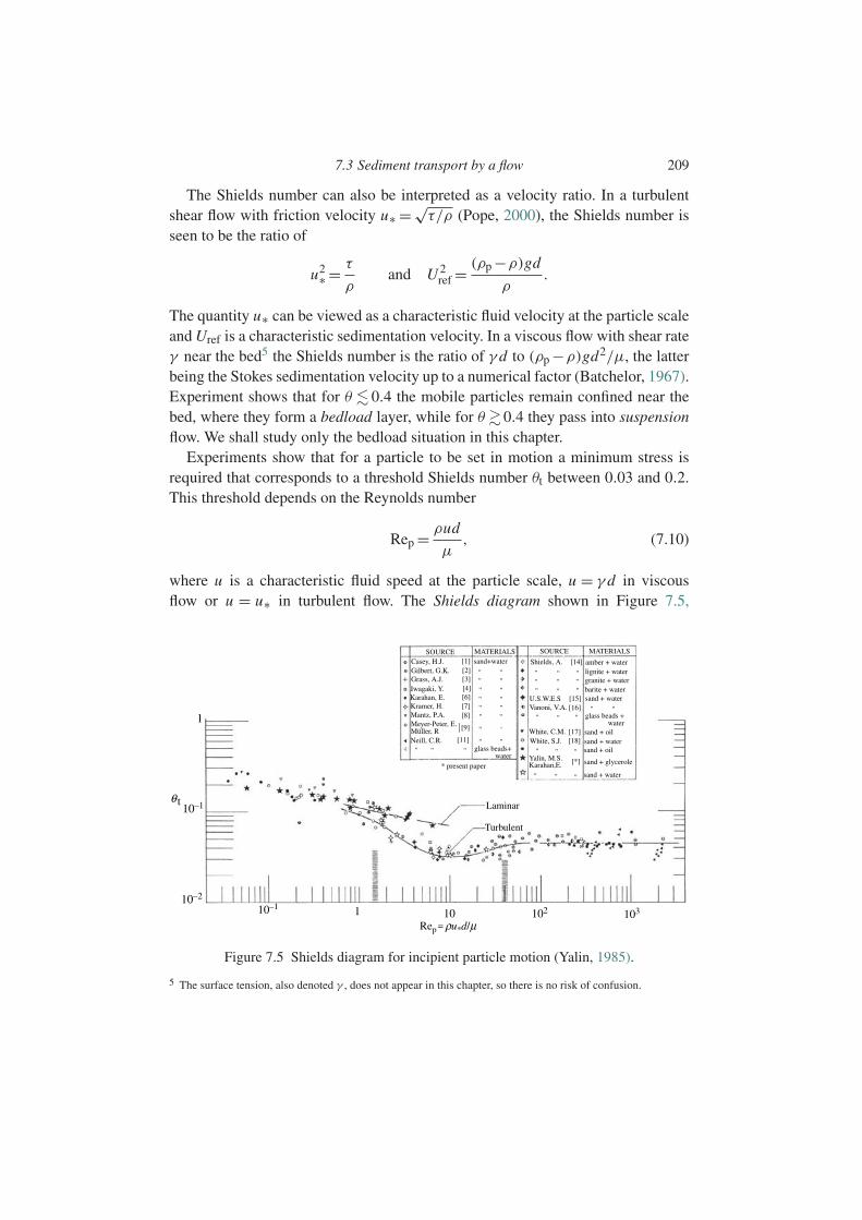
7.3 Sediment transport by a flow 209

The Shields number can also be interpreted as a velocity ratio. In a turbulentshear flow with friction velocity u∗ =√

τ/ρ (Pope, 2000), the Shields number isseen to be the ratio of

u2∗ = τ

ρand U 2

ref =(ρp −ρ)gd

ρ.

The quantity u∗ can be viewed as a characteristic fluid velocity at the particle scaleand Uref is a characteristic sedimentation velocity. In a viscous flow with shear rateγ near the bed5 the Shields number is the ratio of γ d to (ρp −ρ)gd2/µ, the latterbeing the Stokes sedimentation velocity up to a numerical factor (Batchelor, 1967).Experiment shows that for θ 0.4 the mobile particles remain confined near thebed, where they form a bedload layer, while for θ 0.4 they pass into suspensionflow. We shall study only the bedload situation in this chapter.

Experiments show that for a particle to be set in motion a minimum stress isrequired that corresponds to a threshold Shields number θt between 0.03 and 0.2.This threshold depends on the Reynolds number

Rep = ρud

µ, (7.10)

where u is a characteristic fluid speed at the particle scale, u = γ d in viscousflow or u = u∗ in turbulent flow. The Shields diagram shown in Figure 7.5,

Rep=ρu*d/µ

θ t

1

10–1

10–2

10–1102 1031 10

SOURCE MATERIALS SOURCE

[14]

[15][16]

[17][18]

[*]

MATERIALS

Shields, A.

U.S.W.E.SVanoni, V.A.

White, C.M.White, S.J.

Karahan,E.Yalin, M.S.

Casey, H.J.Gilbert, G.K.Grass, A.J.Iwagaki, Y.Karahan, E.Kramer, H.Mantz, P.A.

Neill, C.R.

Laminar

* present paper

Turbulent

Meyer-Peter, E.Müller, R

'' '' glass beads+water

'' '' '''' '''' ''

'' '''' ''

''

''

''

'' ''

''

'' ''''''

''

''''''''''

'

''

''''''''''

''

''''

sand+water[1][2][3][4][6][7][8]

[9]

[11]

amber + waterlignite + watergranite + waterbarite + watersand + water

sand + oilsand + watersand + oil

sand + glycerole

sand + water

glass beads +water

Figure 7.5 Shields diagram for incipient particle motion (Yalin, 1985).

5 The surface tension, also denoted γ , does not appear in this chapter, so there is no risk of confusion.

210 Avalanches, ripples, and dunes

of empirical origin, gives the threshold Shields number θt as a function of theReynolds number Rep.

7.3.2 The speed of mobile particles

Beyond the threshold θt some particles begin to move on the bed surface. Themobile particles form a bedload layer whose thickness, on the order of a fewparticle diameters, increases with the shear. The average speed Up of the parti-cles results from an equilibrium between the force exerted by the flow and theresistence of the bed. In turbulent flow the hydrodynamic force can be written as

1

2C ′

Dρπd2

4(ueff −Up)

2,

where C ′D is a drag coefficient and ueff is an effective speed of the fluid at the

height of a mobile particle. The resistance offered by the bed can be written as aCoulomb friction force

µfmg′,where mg′ is the apparent weight introduced above and µf is a “macroscopic”or “effective” friction coefficient. This coefficient includes not only the frictionat points of particle–particle contact, but also the resistance of geometrical originassociated with the presence of neighboring particles. Setting ueff = α u∗, whereα is a numerical coefficient of order unity, the equilibrium of a particle under theaction of these two forces determines the particle speed (Bagnold, 1973):

Up

Uref=α(

√θ −√θref), Uref =

√(ρp/ρ−1)gd, θref = 4µf

3α2C ′D. (7.11)

Here Uref is a characteristic sedimentation speed and θref is a reference Shieldsnumber below the threshold value θt corresponding to zero particle speed.6 Turbu-lent flow experiments have confirmed the validity of this approach, with α≈5 andθref ≈ 0.8θt (Fernandez Luque and van Beek, 1973; Lajeunesse et al., 2010). Forviscous flow a similar analysis leads to a linear dependence of the velocity Up onthe Shields number (Charru et al., 2007).

The above analysis does not give the friction coefficient itself, but only theratio µf/C ′

D, where C ′D, the particle drag coefficient near a rough wall, is not well

known. The friction coefficient can be estimated from the experiments performedby Bagnold (1954) on the shearing of a suspension of neutrally buoyant particles inCouette flow between two cylinders. It was found in these experiments that the fric-tion coefficient, defined as the ratio of the normal and tangential stresses between

6 The relation (7.11) can also be written as (Up −Upt)/Us =α(√θ −√

θt), where Upt is the minimum particlespeed at threshold.

7.3 Sediment transport by a flow 211

the particles, depends on a modified particle Reynolds number called the Bagnoldnumber, whose expression is not needed here.7 This coefficient decreases mono-tonically from µf =0.75 in the viscous regime to µf =0.32 in the inertial regime.

We conclude by noting that a more rigorous analysis would require measure-ments of the velocity profile inside the mobile layer or direct numerical simulationsof the momentum equations. Such measurements have been performed for vis-cous flow, using a technique of matching the optical indices of the particles andthe fluid (Mouilleron et al., 2009), and reveal a parabolic velocity profile whichis reasonably described by a model inspired by Bagnold (1956). Correspondingmeasurements have not yet been performed for turbulent flow.

Brigadier Ralph Alger Bagnold (1896–1990)

Born in Stoke-Devonport, England, RalphAlger Bagnold had a military career in theRoyal Engineers and Royal Corps of Sig-nals of the British Army, spending longperiods in Egypt and Libya in particu-lar during WWI. An adventurer of insa-tiable curiosity, he acquired great knowl-edge of deserts. After retiring from the armyin 1935, he pursued his observations ofsand transport by wind and water at theHydraulics Laboratory of Imperial Collegein London. In 1941 he published his sec-ond book The Physics of Blown Sand andDesert Dunes, which profoundly influencedthe development of the study of granularmedia. After he was remobilized in 1939 he

was given carte blanche to form a small army, the Long Range Desert Group,that operated in the Libyan desert, carrying out commando operations andobserving the movements of the German Afrika Corps, exploring an immense,largely unknown territory, and making incursions into Chad (where he couldhave encountered Theodore Monod, a Frenchman as unconventional as he was).After WWII he returned to Imperial College, then moved to the United Stateswhere he worked in the U.S. Geological Survey. He published pioneering stud-ies on sediment transport by rivers and oceans and on the physics of granularflow, works which have become standard references in the field. He became a

7 This Bagnold number is analogous to the inertial number I introduced by Forterre and Pouliquen (2008).

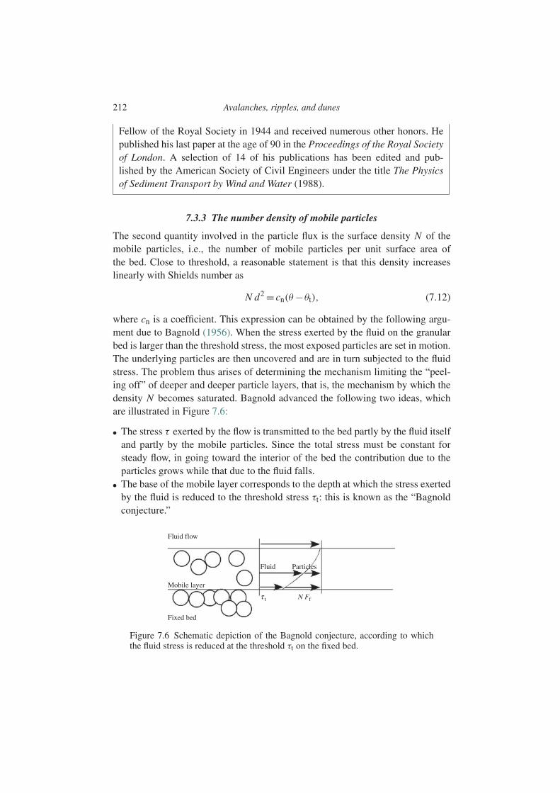
212 Avalanches, ripples, and dunes

Fellow of the Royal Society in 1944 and received numerous other honors. Hepublished his last paper at the age of 90 in the Proceedings of the Royal Societyof London. A selection of 14 of his publications has been edited and pub-lished by the American Society of Civil Engineers under the title The Physicsof Sediment Transport by Wind and Water (1988).

7.3.3 The number density of mobile particles

The second quantity involved in the particle flux is the surface density N of themobile particles, i.e., the number of mobile particles per unit surface area ofthe bed. Close to threshold, a reasonable statement is that this density increaseslinearly with Shields number as

N d2 = cn(θ −θt), (7.12)

where cn is a coefficient. This expression can be obtained by the following argu-ment due to Bagnold (1956). When the stress exerted by the fluid on the granularbed is larger than the threshold stress, the most exposed particles are set in motion.The underlying particles are then uncovered and are in turn subjected to the fluidstress. The problem thus arises of determining the mechanism limiting the “peel-ing off” of deeper and deeper particle layers, that is, the mechanism by which thedensity N becomes saturated. Bagnold advanced the following two ideas, whichare illustrated in Figure 7.6:

• The stress τ exerted by the flow is transmitted to the bed partly by the fluid itselfand partly by the mobile particles. Since the total stress must be constant forsteady flow, in going toward the interior of the bed the contribution due to theparticles grows while that due to the fluid falls.

• The base of the mobile layer corresponds to the depth at which the stress exertedby the fluid is reduced to the threshold stress τt: this is known as the “Bagnoldconjecture.”

Fluid flow

Fluid

τ t N Ff

Particles

Mobile layer

Fixed bed

Figure 7.6 Schematic depiction of the Bagnold conjecture, according to whichthe fluid stress is reduced at the threshold τt on the fixed bed.

7.3 Sediment transport by a flow 213

Assuming as before that the tangential force between the fixed bed and a mobileparticle can be written as µf mg′, we obtain, for N particles per unit surface area,τ − τt = N µf mg′. The relation (7.12) then follows with the identification cn =6/πµf.

According to the arguments by which it was derived, the relation (7.12) mustbe valid for viscous flow (Rep = γ d2/ν 10, τ = µγ ) as well as for turbulentflow (Rep = u∗d/ν 3, τ = ρu2∗). Experiments show that it is well satisfied, withcn =4.6 for turbulent flow (Lajeunesse et al., 2010), and the lower value cn =0.47for viscous flow (Charru et al., 2004). Note that cn < 2 corresponds to values ofµf larger than unity which lead us to doubt the Bagnold conjecture, at least nearthe threshold θt where the few grains in motion at the bed surface occupy only atiny fraction of this surface. Another approach to this problem is discussed in afollowing section.

7.3.4 The particle flux

After finding N and Up, we can obtain the particle flux Q = N Up, i.e., the num-ber of particles crossing a transverse cross-section of the flow per unit time. Forturbulent flow it is given by

Q

Qref= π

6αcn (

√θ −√θref)(θ −θt), Qref = Uref d

πd3/6. (7.13)

This law, where the term√θref is often omitted, agrees fairly well with experiments

with the choice αcn =8–20; however, the measurements show considerable scatter,especially near the threshold. Other empirical laws have been proposed which givesimilar results; one of the most widely used is that of Meyer-Peter and Muller,revised by Wong and Parker (2006):

Q

Qref=3.97(θ −θt)

3/2, θt =0.047. (7.14)

For viscous flow the linear laws for the velocity Up and the density N leadto Q/Qref ∝ θ(θ − θt) as long as the thickness of the mobile layer does notexceed two particle diameters, that is, for θ 3θt (Charru et al., 2004; Mouilleronet al., 2009). Beyond θ ≈ 3θt, a model of viscous resuspension developed byLeighton and Acrivos (1986), which predicts Q/Qref ∝ θ3, is likely to be moreappropriate.

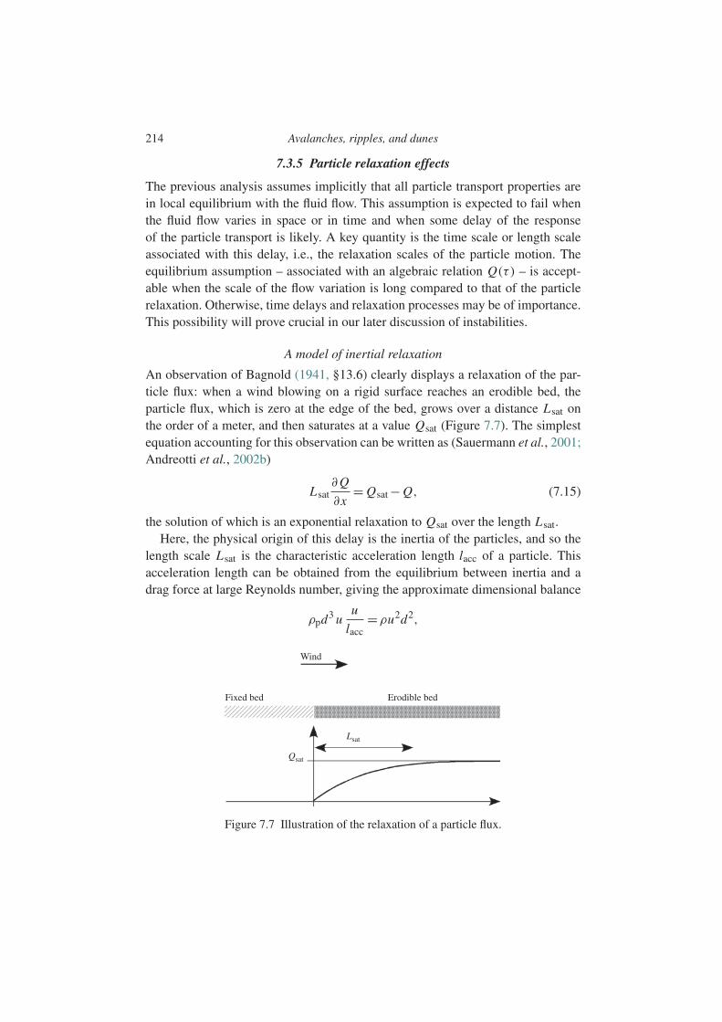
214 Avalanches, ripples, and dunes

7.3.5 Particle relaxation effects

The previous analysis assumes implicitly that all particle transport properties arein local equilibrium with the fluid flow. This assumption is expected to fail whenthe fluid flow varies in space or in time and when some delay of the responseof the particle transport is likely. A key quantity is the time scale or length scaleassociated with this delay, i.e., the relaxation scales of the particle motion. Theequilibrium assumption – associated with an algebraic relation Q(τ ) – is accept-able when the scale of the flow variation is long compared to that of the particlerelaxation. Otherwise, time delays and relaxation processes may be of importance.This possibility will prove crucial in our later discussion of instabilities.

A model of inertial relaxation

An observation of Bagnold (1941, §13.6) clearly displays a relaxation of the par-ticle flux: when a wind blowing on a rigid surface reaches an erodible bed, theparticle flux, which is zero at the edge of the bed, grows over a distance Lsat onthe order of a meter, and then saturates at a value Qsat (Figure 7.7). The simplestequation accounting for this observation can be written as (Sauermann et al., 2001;Andreotti et al., 2002b)

Lsat∂Q

∂x= Qsat − Q, (7.15)

the solution of which is an exponential relaxation to Qsat over the length Lsat.Here, the physical origin of this delay is the inertia of the particles, and so the

length scale Lsat is the characteristic acceleration length lacc of a particle. Thisacceleration length can be obtained from the equilibrium between inertia and adrag force at large Reynolds number, giving the approximate dimensional balance

ρpd3 uu

lacc=ρu2d2,

Wind

Lsat

Qsat

Fixed bed Erodible bed

Figure 7.7 Illustration of the relaxation of a particle flux.

7.3 Sediment transport by a flow 215

where u is the terminal velocity of the particle, equal to the wind velocity. We thusobtain lacc = (ρp/ρ)d. Experiments using sand grains in air effectively show that

Lsat ≈4 lacc =4ρp

ρd, (7.16)

which is about 1.6 m for 0.2 mm grains in air. Equation (7.15) together with theacceleration length (7.16) is an essential element in the analysis of aeolian sanddunes, as will be discussed below. In water, the density of which is a thousandtimes higher than that of air, the acceleration length is of the order of the particlediameter. Viscosity and added mass effects complicate the hydrodynamics in thiscase, and the above analysis is certainly insufficient. The erosion–deposition modelpresented below suggests a more appropriate approach.

An erosion–deposition model

The dynamics of the particle flux can be described using an erosion–depositionmodel of particles at the surface of a sheared bed (Charru et al., 2004). Here weshall consider the case of viscous flow (which is typical of the situations encoun-tered in the oil industry, for example); for the turbulent case, see Lajeunesse et al.(2010). Let N (x, t) be the number of mobile particles per unit surface area andUp(x, t) be their average velocity, so that the particle flux is Q = NUp, as before.Let ne be the erosion rate, that is, the number of particles dislodged from the fixedbed by the flow, per unit time and unit surface area. In the same way, let nd be theparticle deposition rate, i.e., the number of particles stopped in their trajectory byimpact on the fixed bed. The conservation of the number of mobile particles in aslice of thickness dx and unit width, illustrated in Figure 7.8, is then written as

∂N

∂t= ne − nd − ∂Q

∂x, Q = N Up. (7.17)

Fluid flowQ(x)

ηedx

Q(x + dx)

Mobile layer

Fixed bed

. ηddx.

Figure 7.8 Schematic diagram of the particle flux balance in a slice of the mobilelayer of length dx and unit width.

216 Avalanches, ripples, and dunes

The solution of this equation for the density N requires the modeling of the erosionand deposition rates ne and nd, as well as the velocity Up.

The deposition rate nd. The modeling of nd is based on the observation that theparticles move intermittently, with periods of motion at average velocity Up oftypical duration td alternating with periods of rest. During the time td all the par-ticles stop moving at least once on the average, and so the deposition rate can bewritten as

nd = N

td. (7.18)

Deposition is a phenomenon controlled by gravity, and the time td can be assumedto be proportional to the sedimentation time d/Us, where Us is the sedimentationvelocity. Therefore, td can be written as

1

td= cd

Us

d, (7.19)

where cd is a deposition coefficient. For simplicity, in what follows we shall takefor Us the Stokes sedimentation velocity (ρp −ρ)gd2/18µ; other choices are touse the inertial velocity Uref defined by (7.11) or the actual sedimentation velocityas determined by an empirical relation for the drag coefficient.

The erosion rate ne. When the mobile layer is thin, on the order of one or twoparticle diameters, the erosion rate ne depends only on the ability of the flow todislodge a particle from a potential well of characteristic area d2. This rate cantherefore be written as

ne = 1

te d2, (7.20)

where te is a hydrodynamical time scale. For viscous flow this time scale is theinverse of the velocity gradient γ near the bed, from which we find

1

te= ce(γ −γt),

where ce is an erosion coefficient and γt is the velocity gradient at the motionthreshold. Introducing the shear stresses τ =µγ and τt =µγt, the above equationcan be written in a way that is more useful for what follows:

1

te= 1

td

τ −τt

τref, τref = cd

18ce(ρp −ρ)gd. (7.21)

7.3 Sediment transport by a flow 217

The particle speed Up. In the case of viscous flow and small particle inertia,observation shows that the particle speed can be written as Up = cuγ d, where γ dis a characteristic speed of the fluid near the bed and cu is a numerical coefficient,or equivalently

Up

Us=18cu θ. (7.22)

The values of the coefficients measured by Charru et al. (2004) are cd = 0.067,ce =0.0017, and cu =0.10.

Equilibrium solution. The conservation equation (7.17) admits a stationary, uni-form solution for the surface density of mobile particles corresponding to equalityof the erosion and deposition rates (7.18) and (7.20). This solution can be identifiedwith the saturated density

Nsatd2 = td

te=18

ce

cd(θ −θt). (7.23)

Using the expression (7.22) for the particle velocity, for the particle flow rate wefind

Qsat = Nsat Up =182 cuce

cd

Us

d2θ(θ −θt). (7.24)

The flux relaxation equation. We use the above models for the erosion rate (7.20)and the deposition rate (7.18), and assume that the particles have negligible inertiaand move at the velocity (7.22). Then after multiplication by Uptd the conservationequation (7.17) can be written in the form of the relaxation equation

Lsat

(∂N

∂t+ ∂Q

∂x

)= Qsat − Q, (7.25)

where the relaxation length here is defined as

Lsat =Uptd = 1

cd

Up

Usd. (7.26)

Finally, the analysis of erosion and deposition processes provides a relaxationlength scale of the particle transport: this length is associated with the depositionof the particles and corresponds to the length traveled by a particle of velocity Up

during the sedimentation time td.Note that the stationary version of Eq. (7.25) is the same as Eq. (7.15) intro-

duced at the beginning of this section in the context of aeolian transport. However,

218 Avalanches, ripples, and dunes

the physical phenomenon at the origin of the relaxation here is quite different:whereas earlier it was the inertia of the particles accelerated by the flow associ-ated with the acceleration length (7.16), now it is the dynamics of the particledeposition.

7.4 Ripples and dunes: a preliminary dimensional analysis

Before embarking on a detailed analysis we give a brief overview of the structuresobserved on a granular bed sheared by a fluid flow. First we shall discuss ripplesand dunes formed by the wind, and then ripples and dunes formed under water (orequivalently, any liquid).

7.4.1 Aeolian ripples and dunes

When the wind blows on a flat stretch of sand the transported grains form regularripples about 10 cm long (Figure 7.9). The formation mechanism of these ripplesappears to be related to the phenomenon of saltation, i.e., jumps of the sand grainsthat bounce off the bed, are accelerated by the wind, and then fall down again.This saltation motion enhances the momentum transfer from the wind to the bed,that is, it increases the friction. The simple model proposed by Bagnold (1941)

(a)

(b)

Figure 7.9 Sand ripples formed by the wind, from Bagnold (1941): (a) ripplesundergoing formation (one can make out the jumping trajectories of the grains),(b) the final form.

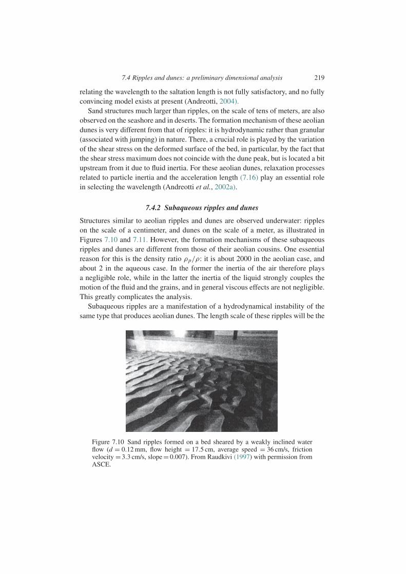
7.4 Ripples and dunes: a preliminary dimensional analysis 219

relating the wavelength to the saltation length is not fully satisfactory, and no fullyconvincing model exists at present (Andreotti, 2004).

Sand structures much larger than ripples, on the scale of tens of meters, are alsoobserved on the seashore and in deserts. The formation mechanism of these aeoliandunes is very different from that of ripples: it is hydrodynamic rather than granular(associated with jumping) in nature. There, a crucial role is played by the variationof the shear stress on the deformed surface of the bed, in particular, by the fact thatthe shear stress maximum does not coincide with the dune peak, but is located a bitupstream from it due to fluid inertia. For these aeolian dunes, relaxation processesrelated to particle inertia and the acceleration length (7.16) play an essential rolein selecting the wavelength (Andreotti et al., 2002a).

7.4.2 Subaqueous ripples and dunes

Structures similar to aeolian ripples and dunes are observed underwater: rippleson the scale of a centimeter, and dunes on the scale of a meter, as illustrated inFigures 7.10 and 7.11. However, the formation mechanisms of these subaqueousripples and dunes are different from those of their aeolian cousins. One essentialreason for this is the density ratio ρp/ρ: it is about 2000 in the aeolian case, andabout 2 in the aqueous case. In the former the inertia of the air therefore playsa negligible role, while in the latter the inertia of the liquid strongly couples themotion of the fluid and the grains, and in general viscous effects are not negligible.This greatly complicates the analysis.

Subaqueous ripples are a manifestation of a hydrodynamical instability of thesame type that produces aeolian dunes. The length scale of these ripples will be the

Figure 7.10 Sand ripples formed on a bed sheared by a weakly inclined waterflow (d = 0.12 mm, flow height = 17.5 cm, average speed = 36 cm/s, frictionvelocity =3.3 cm/s, slope = 0.007). From Raudkivi (1997) with permission fromASCE.

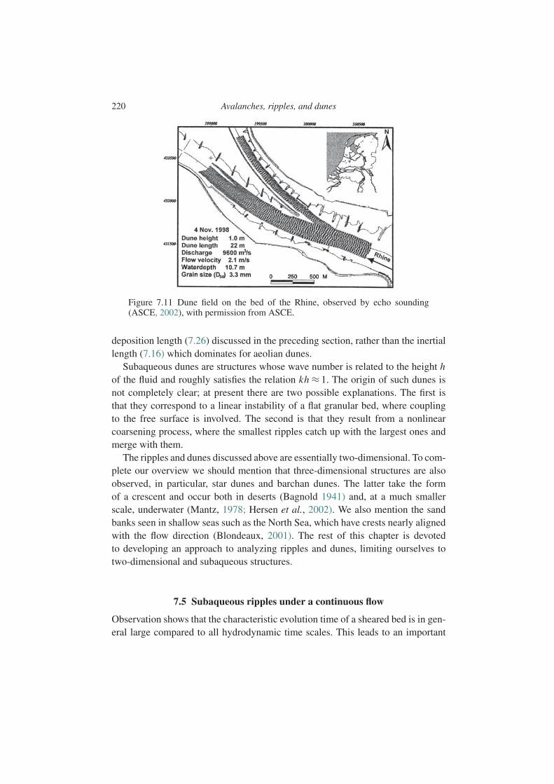
220 Avalanches, ripples, and dunes

Figure 7.11 Dune field on the bed of the Rhine, observed by echo sounding(ASCE, 2002), with permission from ASCE.

deposition length (7.26) discussed in the preceding section, rather than the inertiallength (7.16) which dominates for aeolian dunes.

Subaqueous dunes are structures whose wave number is related to the height hof the fluid and roughly satisfies the relation kh ≈ 1. The origin of such dunes isnot completely clear; at present there are two possible explanations. The first isthat they correspond to a linear instability of a flat granular bed, where couplingto the free surface is involved. The second is that they result from a nonlinearcoarsening process, where the smallest ripples catch up with the largest ones andmerge with them.

The ripples and dunes discussed above are essentially two-dimensional. To com-plete our overview we should mention that three-dimensional structures are alsoobserved, in particular, star dunes and barchan dunes. The latter take the formof a crescent and occur both in deserts (Bagnold 1941) and, at a much smallerscale, underwater (Mantz, 1978; Hersen et al., 2002). We also mention the sandbanks seen in shallow seas such as the North Sea, which have crests nearly alignedwith the flow direction (Blondeaux, 2001). The rest of this chapter is devotedto developing an approach to analyzing ripples and dunes, limiting ourselves totwo-dimensional and subaqueous structures.

7.5 Subaqueous ripples under a continuous flow

Observation shows that the characteristic evolution time of a sheared bed is in gen-eral large compared to all hydrodynamic time scales. This leads to an important

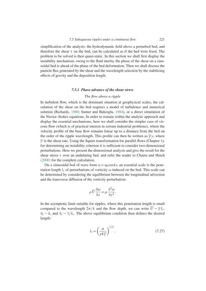
7.5 Subaqueous ripples under a continuous flow 221

simplification of the analysis: the hydrodynamic field above a perturbed bed, andtherefore the shear τ on the bed, can be calculated as if the bed were fixed. Theproblem to be solved is then quasi-static. In this section we shall first display theinstability mechanism: owing to the fluid inertia, the phase of the shear on a sinu-soidal bed is ahead of the phase of the bed deformation. Then we shall discuss theparticle flux generated by the shear and the wavelength selection by the stabilizingeffects of gravity and the deposition length.

7.5.1 Phase advance of the shear stress

The flow above a ripple

In turbulent flow, which is the dominant situation at geophysical scales, the cal-culation of the shear on the bed requires a model of turbulence and numericalsolution (Richards, 1980; Sumer and Bakioglu, 1984), or a direct simulation ofthe Navier–Stokes equations. In order to remain within the analytic approach anddisplay the essential mechanisms, here we shall consider the simpler case of vis-cous flow (which is of practical interest in certain industrial problems), where thevelocity profile of the base flow remains linear up to a distance from the bed onthe order of the ripple wavelength. This profile can then be written as γ y, whereγ is the shear rate. Using the Squire transformation for parallel flows (Chapter 4),for determining an instability criterion it is sufficient to consider two-dimensionalperturbations. Here we present the dimensional analysis and give the result for theshear stress τ over an undulating bed, and refer the reader to Charru and Hinch(2000) for the complete calculation.

On a sinusoidal bed of wave form η= η0 coskx an essential scale is the pene-tration length lv of perturbations of vorticity ω induced on the bed. This scale canbe determined by considering the equilibrium between the longitudinal advectionand the transverse diffusion of the vorticity perturbation:

ρU∂ω

∂x=µ

∂2ω

∂y2.

In the asymptotic limit suitable for ripples, where this penetration length is smallcompared to the wavelength 2π/k and the flow depth, we can write U ∼ γ lv,∂x ∼ k, and ∂y ∼ 1/ lv. The above equilibrium condition then defines the desiredlength:

lv =(

µ

ρkγ

)1/3

. (7.27)

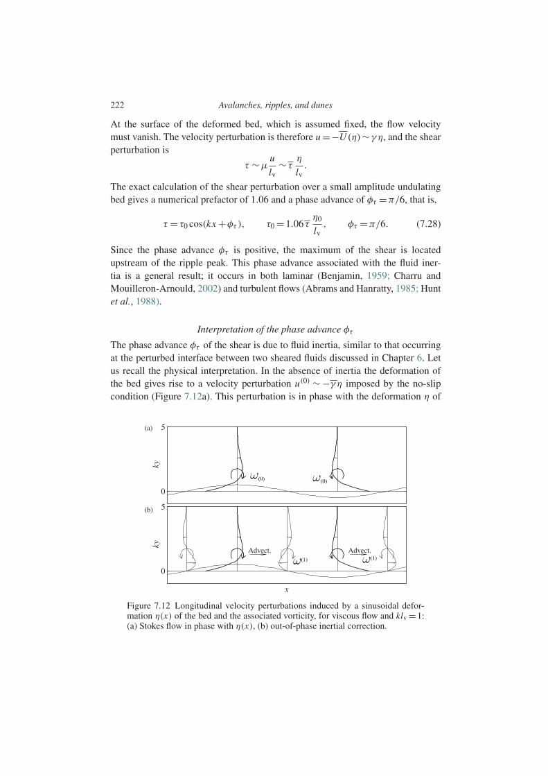
222 Avalanches, ripples, and dunes

At the surface of the deformed bed, which is assumed fixed, the flow velocitymust vanish. The velocity perturbation is therefore u =−U (η)∼γ η, and the shearperturbation is

τ ∼µu

lv∼ τ

η

lv.

The exact calculation of the shear perturbation over a small amplitude undulatingbed gives a numerical prefactor of 1.06 and a phase advance of φτ =π/6, that is,

τ = τ0 cos(kx +φτ ), τ0 =1.06τη0

lv, φτ =π/6. (7.28)

Since the phase advance φτ is positive, the maximum of the shear is locatedupstream of the ripple peak. This phase advance associated with the fluid iner-tia is a general result; it occurs in both laminar (Benjamin, 1959; Charru andMouilleron-Arnould, 2002) and turbulent flows (Abrams and Hanratty, 1985; Huntet al., 1988).

Interpretation of the phase advance φτ

The phase advance φτ of the shear is due to fluid inertia, similar to that occurringat the perturbed interface between two sheared fluids discussed in Chapter 6. Letus recall the physical interpretation. In the absence of inertia the deformation ofthe bed gives rise to a velocity perturbation u(0) ∼ −γ η imposed by the no-slipcondition (Figure 7.12a). This perturbation is in phase with the deformation η of

(a)

(b)

Advect. Advect.

ω(0)

ω(1) ω(1)

ω(0)

Figure 7.12 Longitudinal velocity perturbations induced by a sinusoidal defor-mation η(x) of the bed and the associated vorticity, for viscous flow and klv = 1:(a) Stokes flow in phase with η(x), (b) out-of-phase inertial correction.

7.5 Subaqueous ripples under a continuous flow 223

the bed, as well as the associated vorticity perturbation ω(0) ∼ u(0)/ lv. The shearperturbation of the bed is also in phase with the bed deformation and generates aparticle transport which displaces the ripple without amplifying it. The correctioninduced by weak inertial effects corresponds to advection of the vorticity perturba-tion ω(0) by the base flow. This advection creates a component ω(1)∼Reeffω

(0) outof phase with the bed deformation, where Reeff = γ l2

v/ν is an effective Reynoldsnumber. The velocity field u(1) ∼ω(1)lv associated with ω(1) must vanish on thebed, and corresponds to the out-of-phase profile sketched in Figure 7.12b. Theshear τ (1) ∼µu(1)/ lv associated with this inertial correction therefore points fromthe troughs toward the peaks, hence reinforcing the advancement of the phase,resulting in instability.

7.5.2 Instability

Stability analyses of erodible beds have for a long time been based on algebraicparticle transport laws of the type Q = Q(τ ) established for stationary, uniformflow, such as the Meyer-Peter–Muller law (7.14). The inclusion of the relaxation ofthe particle flux in a spatially varying shear significantly modifies the results. Herewe shall discuss the stability within the context of the erosion–deposition modelpresented in the preceding section, while restricting our analysis to viscous flow.

The particle flux

For stationary and uniform flow, the surface density N of mobile particles andflux Q correspond to the equilibrium solution (7.23) and (7.24) of the erosion–deposition model with the particle velocity (7.22). On a wavy bed with wave formη = η0 coskx , the shear perturbation τ induces a perturbation up of the particlevelocity given by

up =U ′p(τ )τ, where U ′

p(τ )=∂Up

∂τ(τ ). (7.29)

The perturbation n of the surface density of mobile particles is the solution of theconservation equation (7.17), the linearized form of which is written as

0=−nd2 + τ

τref− tdd2 ∂q

∂x, q = N U ′

p(τ )τ +U p n, (7.30)

where q is the perturbation of the particle flux and for consistency with the quasi-static approximation for the flow we have neglected the time derivative.8 Seeking

8 An additional justification for this omission is that the term ∂t n is dominated by the propagation of the rippleat speed c, and not by its slow growth, so that ∂t n ≈−c∂x n. Since c Up, we deduce that ∂t n is negligiblecompared to the term Up ∂x n on the right-hand side of (7.30).

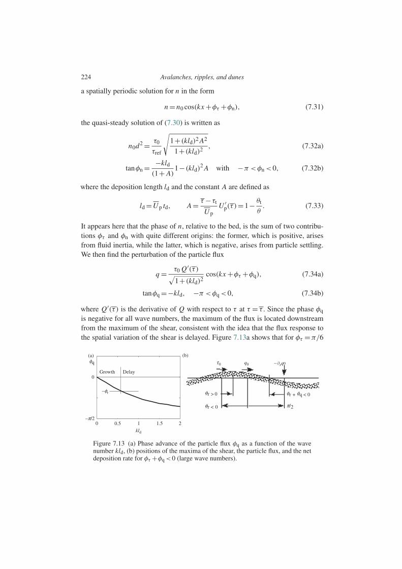
224 Avalanches, ripples, and dunes

a spatially periodic solution for n in the form

n =n0 cos(kx +φτ +φn), (7.31)

the quasi-steady solution of (7.30) is written as

n0d2 = τ0

τref

√1+(kld)2 A2

1+(kld)2, (7.32a)

tanφn = −kld

(1+ A)1−(kld)

2 A with −π <φn <0, (7.32b)

where the deposition length ld and the constant A are defined as

ld =U p td, A = τ −τt

U pU ′

p(τ )=1− θt

θ. (7.33)

It appears here that the phase of n, relative to the bed, is the sum of two contribu-tions φτ and φn with quite different origins: the former, which is positive, arisesfrom fluid inertia, while the latter, which is negative, arises from particle settling.We then find the perturbation of the particle flux

q = τ0 Q′(τ )√1+(kld)2

cos(kx +φτ +φq), (7.34a)

tanφq =−kld, −π <φq <0, (7.34b)

where Q′(τ ) is the derivative of Q with respect to τ at τ = τ . Since the phase φq

is negative for all wave numbers, the maximum of the flux is located downstreamfrom the maximum of the shear, consistent with the idea that the flux response tothe spatial variation of the shear is delayed. Figure 7.13a shows that for φτ =π/6

Figure 7.13 (a) Phase advance of the particle flux φq as a function of the wavenumber kld, (b) positions of the maxima of the shear, the particle flux, and the netdeposition rate for φτ +φq <0 (large wave numbers).

7.5 Subaqueous ripples under a continuous flow 225

(see Eq. (7.28)), small wave numbers correspond to φτ +φq >0 and so the particleflux is ahead of the bed deformation, while the opposite occurs for large wavenumbers. The cutoff wave number koff is such that φτ +φq =0, or

koffld = tanφτ . (7.35)

Since the net deposition rate on a section of length dx and unit width is Q(x)−Q(x +dx)=−∂xq dx , the quasi-static evolution of the bed is governed by the massconservation equation

∂η

∂t=−πd3

6C

∂q

∂x= πd3

6C(nd − ne), (7.36)

where C ≈0.6 is the compactness of the bed (the volume fraction occupied by theparticles). This evolution equation is closed using Eq. (7.34) for the particle flux.Figure 7.13b illustrates the case of large wave numbers for which φτ +φq <0. Thiscase corresponds to net erosion of the peaks and deposition in the troughs, that is,damped perturbations. We note that if particle relaxation is neglected [Q = Q(τ )],the particle flux is in phase with the shear (ld = 0, φq = 0) and all wave numbersare unstable (with φτ >0).

The effect of gravity

On a bed of slope ∂xη the particle flux is affected by the component of gravity par-allel to the slope. The corresponding force (ρp −ρ)g ∂xη per unit particle volumetends to shift the particles from the peaks toward the troughs and plays a stabiliz-ing role. Assuming that the thickness of the mobile layer is approximately d, thisforce can be taken into account by replacing the shear stress τ by an “effective”stress defined as9

τeff = τ −cg(ρp −ρ)gd ∂xη, (7.37)

where cg is a numerical coefficient. Equivalently, the effect of gravity can be takeninto account by an effective threshold for the start of the motion:

τt,eff = τt +cg(ρp −ρ)gd ∂xη= τt (1+(cg/θt )∂xη). (7.38)

A slope also directly affects the threshold τt for the particles to start moving: thethreshold is increased for a positive slope and decreased for a negative slope. In

9 The force per unit surface area due to gravity should grow with the thickness of the mobile layer and thereforewith the Shields number. One method of taking this growth into account which is consistent with (7.12) is tomultiply the correction of τ in (7.37) by (θ − θt)/θt. The conclusions of the analysis are not fundamentallychanged.

226 Avalanches, ripples, and dunes

fact, this second effect of the slope can be assumed to be included in the coefficientcg introduced above. This coefficient plays an essential role in the selection ofthe most amplified wavelength, but unfortunately its value remains uncertain; ingeneral, it is chosen to lie between 0.1 and 0.4.

We can therefore consider that the density of mobile particles (7.32) and the flux(7.34) include the effect of gravity when τ0 and φτ are replaced by the amplitudeand the phase of the effective shear (7.37).

The speed and growth rate

The speed and the growth rate of the ripples are finally obtained from the massconservation equation (7.36) with η=η0 eσ t cosk(x −ct). We find

c = πd3

6CQ′(τ )

τ0

η0cosφq cos(φτ +φq), (7.39a)

σ = πd3

6CQ′(τ )cos2 φq

(kτ0

η0

sin(φτ +φq)

cosφq−cg (ρp −ρ)gd k2

). (7.39b)

Let us make the following comments about these results:

• The above expressions for the speed and the growth rate are general; the precisenature of the flow – viscous or turbulent – is “encoded” in τ0 and φτ , while thatof the particle transport is encoded in Q′(τ ) and φq.

• The equilibrium transport law Q= Q(τ ) does not affect the stability or instabilityof the bed, but only the values of the speed and the growth rate.

• The particle relaxation introduced via the erosion–deposition model leads tothe appearance of the deposition length ld; a purely algebraic transport lawcorresponds to ld =0.

• The stabilizing particle relaxation and gravity effects are weak at small wavenumbers, where the destabilizing fluid inertia dominates, while they dominate atlarge wave numbers.

The general shape of the curve for the growth rate σ(k) corresponds to thatof a long-wavelength instability already encountered several times in precedingchapters. The unstable wave numbers lie below a cutoff koff, the stable ones lieabove it, and there exists a maximally amplified wave number kmax between k =0(neutral) and k = koff. Figure 7.14 shows the behavior of kmaxd as a function ofthe Shields number for viscous shear (7.28) and the particle transport law (7.24).When the stabilizing mechanism due to gravity is the only one taken into account(ld = 0), kmaxd varies as θ2 (dashed lines, for two values of the sedimentationReynolds number Res =ρUsd/µ). Conversely, when the stabilizing mechanism of

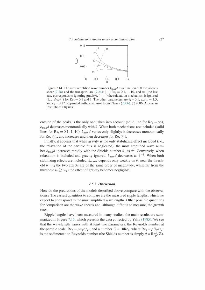
7.5 Subaqueous ripples under a continuous flow 227

k max

d

0.11

10

1

0.1

Figure 7.14 The most amplified wave number kmaxd as a function of θ for viscousshear (7.28) and the transport law (7.24): (—) Res = 0.1, 1, 10, and ∞ (the lastcase corresponds to ignoring gravity), (– – –) the relaxation mechanism is ignored(kmaxd ∝ θ2) for Res = 0.1 and 1. The other parameters are θt = 0.1, cu/cd = 1.5,and cg = 0.17. Reprinted with permission from Charru (2006). c© 2006, AmericanInstitute of Physics.

erosion of the peaks is the only one taken into account (solid line for Res = ∞),kmaxd decreases monotonically with θ . When both mechanisms are included (solidlines for Res = 0.1, 1, 10), kmaxd varies only slightly: it decreases monotonicallyfor Res 1, and increases and then decreases for Res 1.

Finally, it appears that when gravity is the only stabilizing effect included (i.e.,the relaxation of the particle flux is neglected), the most amplified wave num-ber kmaxd increases rapidly with the Shields number θ , as θ2. Conversely, whenrelaxation is included and gravity ignored, kmaxd decreases as θ−1. When bothstabilizing effects are included, kmaxd depends only weakly on θ ; near the thresh-old θ = θt the two effects are of the same order of magnitude, while far from thethreshold (θ 3θt ) the effect of gravity becomes negligible.

7.5.3 Discussion

How do the predictions of the models described above compare with the observa-tions? The easiest quantities to compare are the measured ripple lengths, which weexpect to correspond to the most amplified wavelengths. Other possible quantitiesfor comparison are the wave speeds and, although difficult to measure, the growthrates.

Ripple lengths have been measured in many studies; the main results are sum-marized in Figure 7.15, which presents the data collected by Yalin (1985). We seethat the wavelength varies with at least two parameters: the Reynolds number atthe particle scale, Rep =ρu∗d/µ, and a number !=18Res, where Res =ρUsd/µis the sedimentation Reynolds number (the Shields number is simply θ =Re2

p/!).

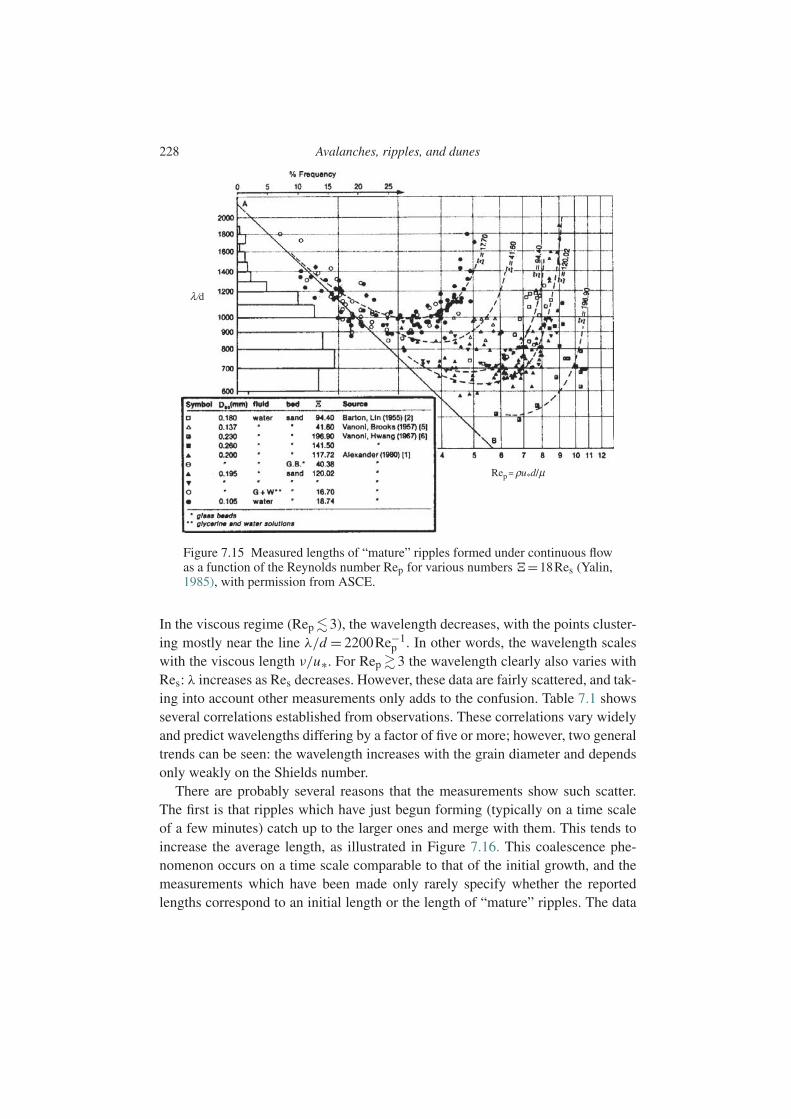
228 Avalanches, ripples, and dunes

Rep=ρu*d/µ

λ/d

Figure 7.15 Measured lengths of “mature” ripples formed under continuous flowas a function of the Reynolds number Rep for various numbers !=18Res (Yalin,1985), with permission from ASCE.

In the viscous regime (Rep 3), the wavelength decreases, with the points cluster-ing mostly near the line λ/d = 2200Re−1

p . In other words, the wavelength scaleswith the viscous length ν/u∗. For Rep 3 the wavelength clearly also varies withRes: λ increases as Res decreases. However, these data are fairly scattered, and tak-ing into account other measurements only adds to the confusion. Table 7.1 showsseveral correlations established from observations. These correlations vary widelyand predict wavelengths differing by a factor of five or more; however, two generaltrends can be seen: the wavelength increases with the grain diameter and dependsonly weakly on the Shields number.

There are probably several reasons that the measurements show such scatter.The first is that ripples which have just begun forming (typically on a time scaleof a few minutes) catch up to the larger ones and merge with them. This tends toincrease the average length, as illustrated in Figure 7.16. This coalescence phe-nomenon occurs on a time scale comparable to that of the initial growth, and themeasurements which have been made only rarely specify whether the reportedlengths correspond to an initial length or the length of “mature” ripples. The data

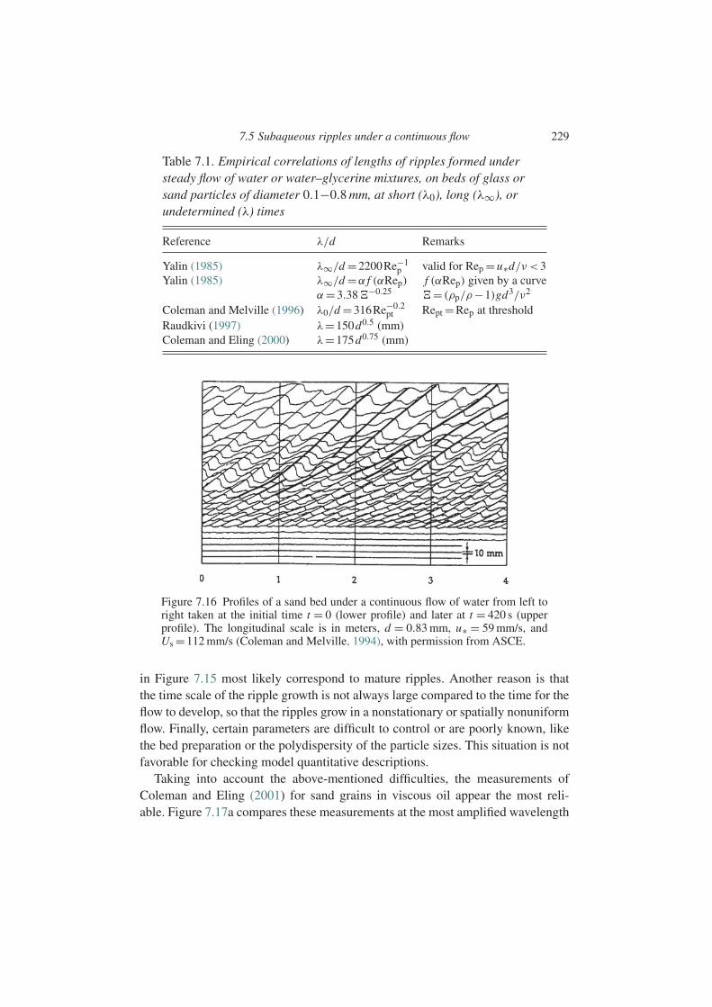
7.5 Subaqueous ripples under a continuous flow 229

Table 7.1. Empirical correlations of lengths of ripples formed understeady flow of water or water–glycerine mixtures, on beds of glass orsand particles of diameter 0.1−0.8 mm, at short (λ0), long (λ∞), orundetermined (λ) times

Reference λ/d Remarks

Yalin (1985) λ∞/d =2200Re−1p valid for Rep =u∗d/ν <3

Yalin (1985) λ∞/d =α f (αRep) f (αRep) given by a curveα=3.38!−0.25 != (ρp/ρ−1)gd3/ν2

Coleman and Melville (1996) λ0/d =316Re−0.2pt Rept =Rep at threshold

Raudkivi (1997) λ=150d0.5 (mm)Coleman and Eling (2000) λ=175d0.75 (mm)

Figure 7.16 Profiles of a sand bed under a continuous flow of water from left toright taken at the initial time t = 0 (lower profile) and later at t = 420 s (upperprofile). The longitudinal scale is in meters, d = 0.83 mm, u∗ = 59 mm/s, andUs =112 mm/s (Coleman and Melville, 1994), with permission from ASCE.

in Figure 7.15 most likely correspond to mature ripples. Another reason is thatthe time scale of the ripple growth is not always large compared to the time for theflow to develop, so that the ripples grow in a nonstationary or spatially nonuniformflow. Finally, certain parameters are difficult to control or are poorly known, likethe bed preparation or the polydispersity of the particle sizes. This situation is notfavorable for checking model quantitative descriptions.

Taking into account the above-mentioned difficulties, the measurements ofColeman and Eling (2001) for sand grains in viscous oil appear the most reli-able. Figure 7.17a compares these measurements at the most amplified wavelength

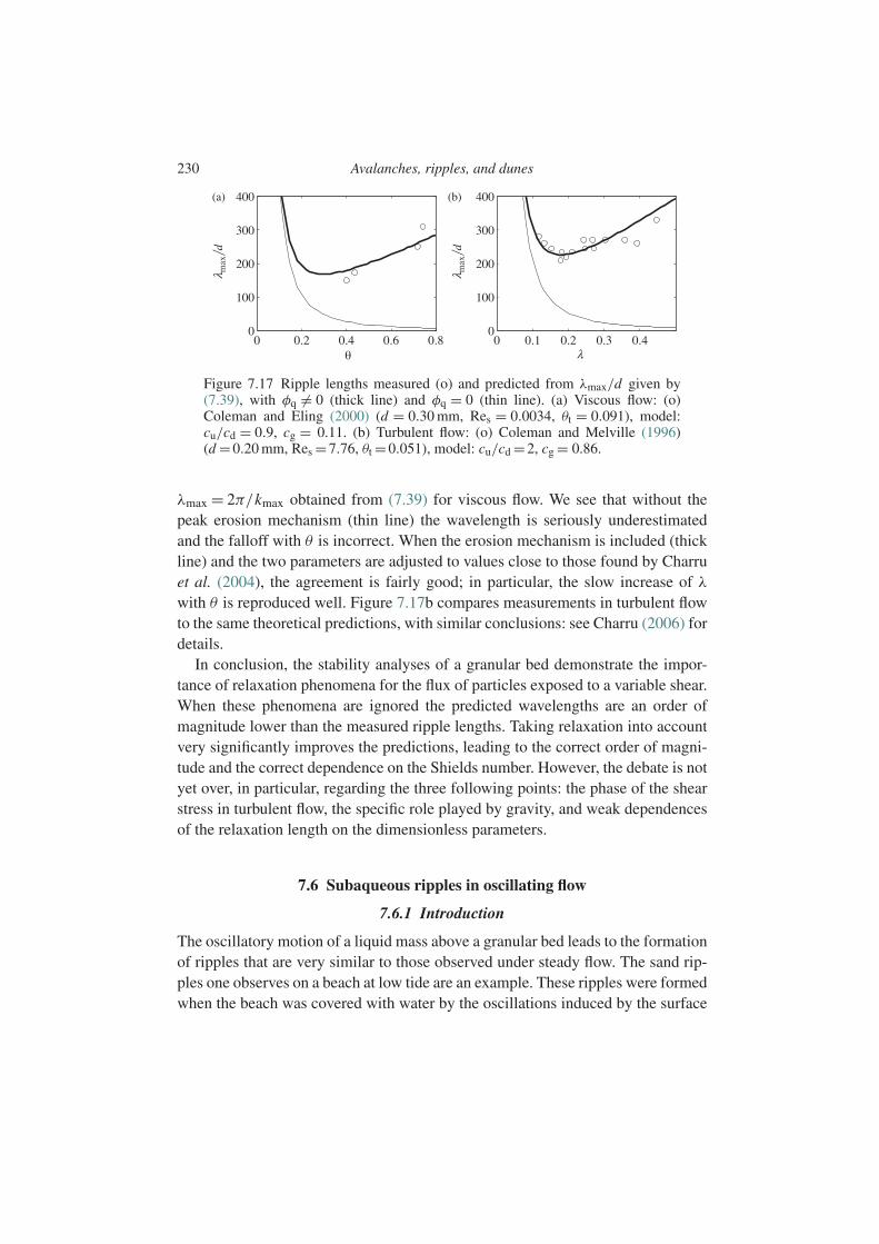
230 Avalanches, ripples, and dunes

λ

λ max

/d

λ max

/d

(a) (b)

Figure 7.17 Ripple lengths measured (o) and predicted from λmax/d given by(7.39), with φq = 0 (thick line) and φq = 0 (thin line). (a) Viscous flow: (o)Coleman and Eling (2000) (d = 0.30 mm, Res = 0.0034, θt = 0.091), model:cu/cd = 0.9, cg = 0.11. (b) Turbulent flow: (o) Coleman and Melville (1996)(d =0.20 mm, Res =7.76, θt =0.051), model: cu/cd =2, cg = 0.86.

λmax = 2π/kmax obtained from (7.39) for viscous flow. We see that without thepeak erosion mechanism (thin line) the wavelength is seriously underestimatedand the falloff with θ is incorrect. When the erosion mechanism is included (thickline) and the two parameters are adjusted to values close to those found by Charruet al. (2004), the agreement is fairly good; in particular, the slow increase of λwith θ is reproduced well. Figure 7.17b compares measurements in turbulent flowto the same theoretical predictions, with similar conclusions: see Charru (2006) fordetails.

In conclusion, the stability analyses of a granular bed demonstrate the impor-tance of relaxation phenomena for the flux of particles exposed to a variable shear.When these phenomena are ignored the predicted wavelengths are an order ofmagnitude lower than the measured ripple lengths. Taking relaxation into accountvery significantly improves the predictions, leading to the correct order of magni-tude and the correct dependence on the Shields number. However, the debate is notyet over, in particular, regarding the three following points: the phase of the shearstress in turbulent flow, the specific role played by gravity, and weak dependencesof the relaxation length on the dimensionless parameters.

7.6 Subaqueous ripples in oscillating flow

7.6.1 Introduction

The oscillatory motion of a liquid mass above a granular bed leads to the formationof ripples that are very similar to those observed under steady flow. The sand rip-ples one observes on a beach at low tide are an example. These ripples were formedwhen the beach was covered with water by the oscillations induced by the surface

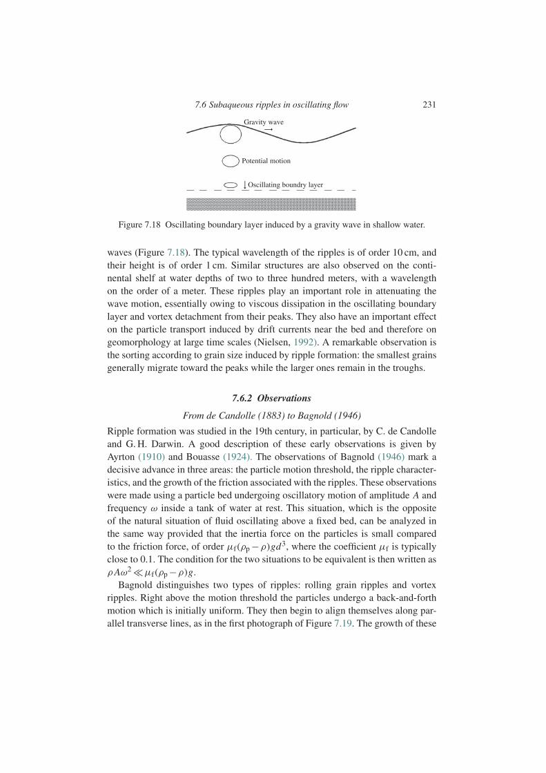
7.6 Subaqueous ripples in oscillating flow 231

Gravity wave

Potential motion

Oscillating boundry layer

Figure 7.18 Oscillating boundary layer induced by a gravity wave in shallow water.

waves (Figure 7.18). The typical wavelength of the ripples is of order 10 cm, andtheir height is of order 1 cm. Similar structures are also observed on the conti-nental shelf at water depths of two to three hundred meters, with a wavelengthon the order of a meter. These ripples play an important role in attenuating thewave motion, essentially owing to viscous dissipation in the oscillating boundarylayer and vortex detachment from their peaks. They also have an important effecton the particle transport induced by drift currents near the bed and therefore ongeomorphology at large time scales (Nielsen, 1992). A remarkable observation isthe sorting according to grain size induced by ripple formation: the smallest grainsgenerally migrate toward the peaks while the larger ones remain in the troughs.

7.6.2 Observations

From de Candolle (1883) to Bagnold (1946)

Ripple formation was studied in the 19th century, in particular, by C. de Candolleand G. H. Darwin. A good description of these early observations is given byAyrton (1910) and Bouasse (1924). The observations of Bagnold (1946) mark adecisive advance in three areas: the particle motion threshold, the ripple character-istics, and the growth of the friction associated with the ripples. These observationswere made using a particle bed undergoing oscillatory motion of amplitude A andfrequency ω inside a tank of water at rest. This situation, which is the oppositeof the natural situation of fluid oscillating above a fixed bed, can be analyzed inthe same way provided that the inertia force on the particles is small comparedto the friction force, of order µf(ρp −ρ)gd3, where the coefficient µf is typicallyclose to 0.1. The condition for the two situations to be equivalent is then written asρAω2 µf(ρp −ρ)g.

Bagnold distinguishes two types of ripples: rolling grain ripples and vortexripples. Right above the motion threshold the particles undergo a back-and-forthmotion which is initially uniform. They then begin to align themselves along par-allel transverse lines, as in the first photograph of Figure 7.19. The growth of these

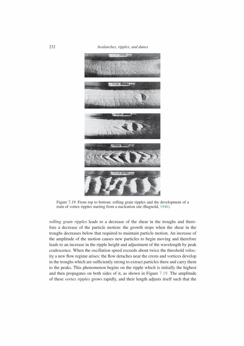
232 Avalanches, ripples, and dunes

Figure 7.19 From top to bottom: rolling grain ripples and the development of atrain of vortex ripples starting from a nucleation site (Bagnold, 1946).

rolling grain ripples leads to a decrease of the shear in the troughs and there-fore a decrease of the particle motion: the growth stops when the shear in thetroughs decreases below that required to maintain particle motion. An increase ofthe amplitude of the motion causes new particles to begin moving and thereforeleads to an increase in the ripple height and adjustment of the wavelength by peakcoalescence. When the oscillation speed exceeds about twice the threshold veloc-ity a new flow regime arises: the flow detaches near the crests and vortices developin the troughs which are sufficiently strong to extract particles there and carry themto the peaks. This phenomenon begins on the ripple which is initially the highestand then propagates on both sides of it, as shown in Figure 7.19. The amplitudeof these vortex ripples grows rapidly, and their length adjusts itself such that the

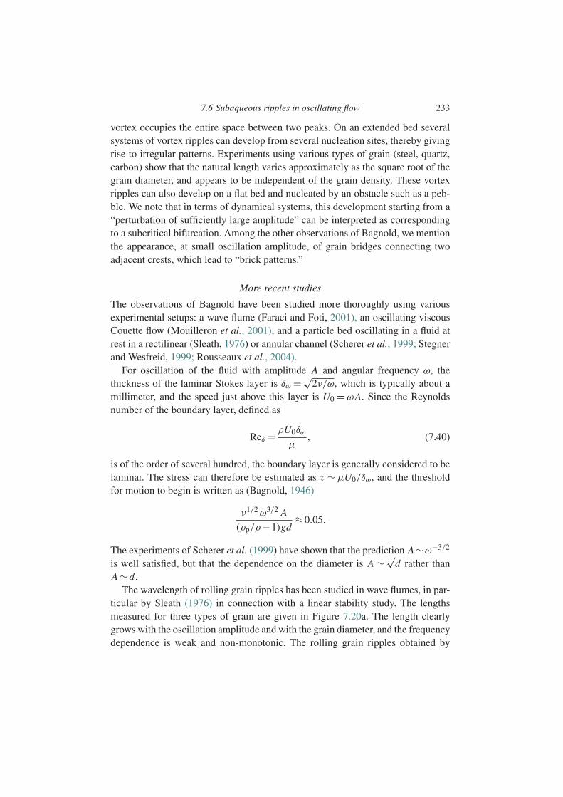
7.6 Subaqueous ripples in oscillating flow 233

vortex occupies the entire space between two peaks. On an extended bed severalsystems of vortex ripples can develop from several nucleation sites, thereby givingrise to irregular patterns. Experiments using various types of grain (steel, quartz,carbon) show that the natural length varies approximately as the square root of thegrain diameter, and appears to be independent of the grain density. These vortexripples can also develop on a flat bed and nucleated by an obstacle such as a peb-ble. We note that in terms of dynamical systems, this development starting from a“perturbation of sufficiently large amplitude” can be interpreted as correspondingto a subcritical bifurcation. Among the other observations of Bagnold, we mentionthe appearance, at small oscillation amplitude, of grain bridges connecting twoadjacent crests, which lead to “brick patterns.”

More recent studies

The observations of Bagnold have been studied more thoroughly using variousexperimental setups: a wave flume (Faraci and Foti, 2001), an oscillating viscousCouette flow (Mouilleron et al., 2001), and a particle bed oscillating in a fluid atrest in a rectilinear (Sleath, 1976) or annular channel (Scherer et al., 1999; Stegnerand Wesfreid, 1999; Rousseaux et al., 2004).

For oscillation of the fluid with amplitude A and angular frequency ω, thethickness of the laminar Stokes layer is δω = √

2ν/ω, which is typically about amillimeter, and the speed just above this layer is U0 = ωA. Since the Reynoldsnumber of the boundary layer, defined as

Reδ = ρU0δω

µ, (7.40)

is of the order of several hundred, the boundary layer is generally considered to belaminar. The stress can therefore be estimated as τ ∼µU0/δω, and the thresholdfor motion to begin is written as (Bagnold, 1946)

ν1/2 ω3/2 A

(ρp/ρ−1)gd≈0.05.

The experiments of Scherer et al. (1999) have shown that the prediction A∼ω−3/2

is well satisfied, but that the dependence on the diameter is A ∼ √d rather than

A ∼d.The wavelength of rolling grain ripples has been studied in wave flumes, in par-

ticular by Sleath (1976) in connection with a linear stability study. The lengthsmeasured for three types of grain are given in Figure 7.20a. The length clearlygrows with the oscillation amplitude and with the grain diameter, and the frequencydependence is weak and non-monotonic. The rolling grain ripples obtained by

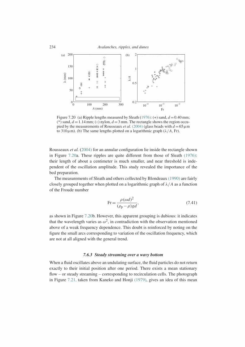
234 Avalanches, ripples, and dunes

Fr

(a) (b)

Figure 7.20 (a) Ripple lengths measured by Sleath (1976): (+) sand, d =0.40 mm;(*) sand, d =1.14 mm; () nylon, d =3 mm. The rectangle shows the region occu-pied by the measurements of Rousseaux et al. (2004) (glass beads with d =65 µmto 310µm). (b) The same lengths plotted on a logarithmic graph (λ/A, Fr).

Rousseaux et al. (2004) for an annular configuration lie inside the rectangle shownin Figure 7.20a. These ripples are quite different from those of Sleath (1976):their length of about a centimeter is much smaller, and near threshold is inde-pendent of the oscillation amplitude. This study revealed the importance of thebed preparation.

The measurements of Sleath and others collected by Blondeaux (1990) are fairlyclosely grouped together when plotted on a logarithmic graph of λ/A as a functionof the Froude number

Fr= ρ(ωd)2

(ρp −ρ)gd, (7.41)

as shown in Figure 7.20b. However, this apparent grouping is dubious: it indicatesthat the wavelength varies as ω2, in contradiction with the observation mentionedabove of a weak frequency dependence. This doubt is reinforced by noting on thefigure the small arcs corresponding to variation of the oscillation frequency, whichare not at all aligned with the general trend.

7.6.3 Steady streaming over a wavy bottom

When a fluid oscillates above an undulating surface, the fluid particles do not returnexactly to their initial position after one period. There exists a mean stationaryflow – or steady streaming – corresponding to recirculation cells. The photographin Figure 7.21, taken from Kaneko and Honji (1979), gives an idea of this mean

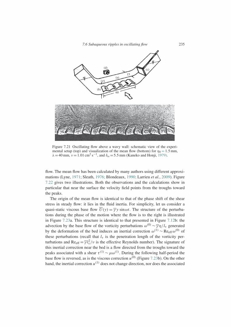
7.6 Subaqueous ripples in oscillating flow 235

(d)

(b)

(a)15

15

60

(c)

Figure 7.21 Oscillating flow above a wavy wall: schematic view of the experi-mental setup (top) and visualization of the mean flow (bottom) for η0 = 1.5 mm,λ=40 mm, ν =1.01 cm2 s−1, and δω =5.5 mm (Kaneko and Honji, 1979).

flow. The mean flow has been calculated by many authors using different approxi-mations (Lyne, 1971; Sleath, 1976; Blondeaux, 1990; Larrieu et al., 2009). Figure7.22 gives two illustrations. Both the observations and the calculations show inparticular that near the surface the velocity field points from the troughs towardthe peaks.

The origin of the mean flow is identical to that of the phase shift of the shearstress in steady flow: it lies in the fluid inertia. For simplicity, let us consider aquasi-static viscous base flow U (y) = γ y sinωt . The structure of the perturba-tions during the phase of the motion where the flow is to the right is illustratedin Figure 7.23a. This structure is identical to that presented in Figure 7.12b: theadvection by the base flow of the vorticity perturbations ω(0) ∼ γ η/ lv generatedby the deformation of the bed induces an inertial correction ω(1) ∼ Reeff ω

(0) ofthese perturbations (recall that lv is the penetration length of the vorticity per-turbations and Reeff = γ l2

v/ν is the effective Reynolds number). The signature ofthis inertial correction near the bed is a flow directed from the troughs toward thepeaks associated with a shear τ (1) ∼µω(1). During the following half-period thebase flow is reversed, as is the viscous correction u(0) (Figure 7.23b). On the otherhand, the inertial correction u(1) does not change direction, nor does the associated

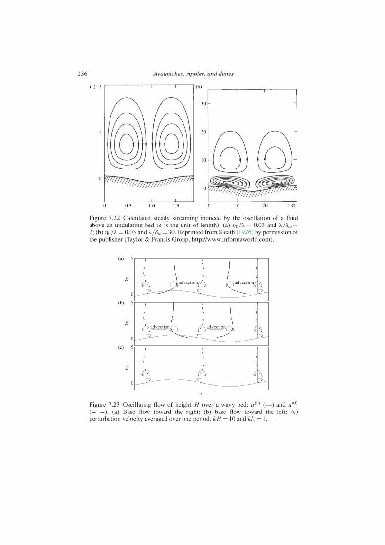
236 Avalanches, ripples, and dunes

2 (b)(a)

1

0

0 0.5 1.51.0 0 10

30

20

0

10

3020

Figure 7.22 Calculated steady streaming induced by the oscillation of a fluidabove an undulating bed (δ is the unit of length): (a) η0/λ = 0.03 and λ/δω =2; (b) η0/λ= 0.03 and λ/δω =30. Reprinted from Sleath (1976) by permission ofthe publisher (Taylor & Francis Group, http://www.informaworld.com).

(a)

(b)

(c)

Figure 7.23 Oscillating flow of height H over a wavy bed: u(0) (—) and u(0)

(− −). (a) Base flow toward the right; (b) base flow toward the left; (c)perturbation velocity averaged over one period. k H =10 and klv =1.

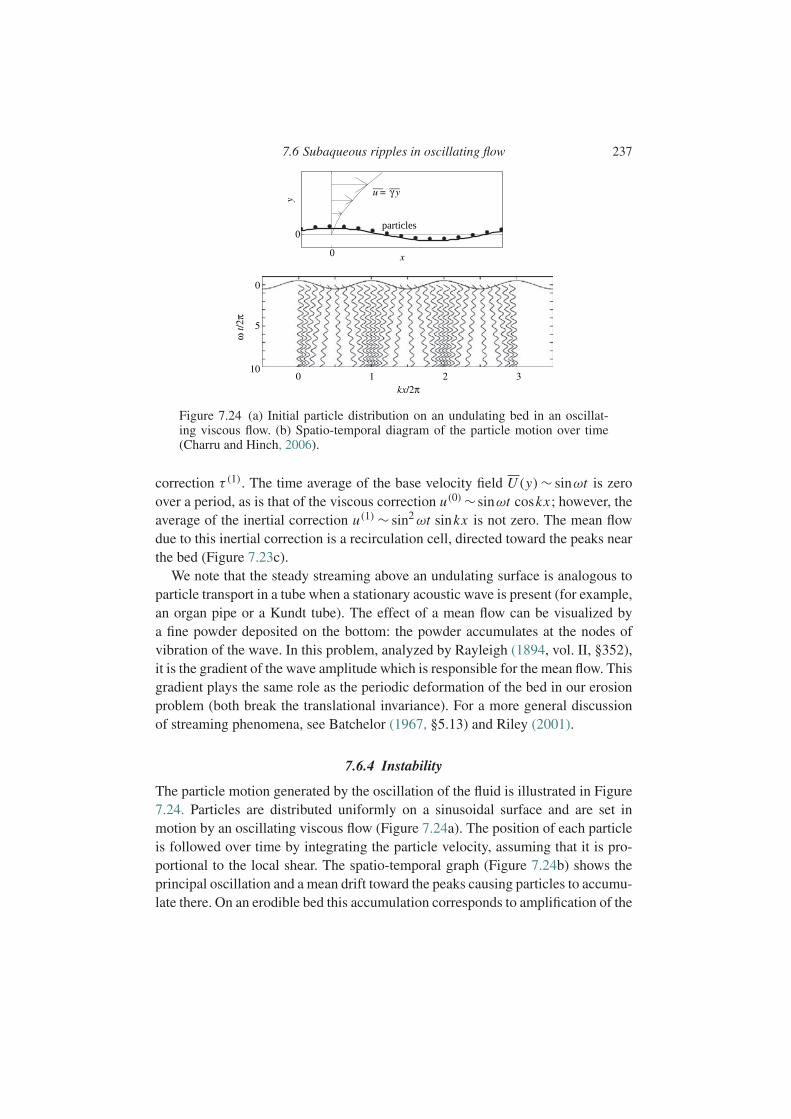
7.6 Subaqueous ripples in oscillating flow 237

0

0

u = γ y— —

particles

y

x

0

5

0 1 2kx/2π

ω t/

2π

310

Figure 7.24 (a) Initial particle distribution on an undulating bed in an oscillat-ing viscous flow. (b) Spatio-temporal diagram of the particle motion over time(Charru and Hinch, 2006).

correction τ (1). The time average of the base velocity field U (y)∼ sinωt is zeroover a period, as is that of the viscous correction u(0) ∼ sinωt coskx ; however, theaverage of the inertial correction u(1) ∼ sin2 ωt sinkx is not zero. The mean flowdue to this inertial correction is a recirculation cell, directed toward the peaks nearthe bed (Figure 7.23c).

We note that the steady streaming above an undulating surface is analogous toparticle transport in a tube when a stationary acoustic wave is present (for example,an organ pipe or a Kundt tube). The effect of a mean flow can be visualized bya fine powder deposited on the bottom: the powder accumulates at the nodes ofvibration of the wave. In this problem, analyzed by Rayleigh (1894, vol. II, §352),it is the gradient of the wave amplitude which is responsible for the mean flow. Thisgradient plays the same role as the periodic deformation of the bed in our erosionproblem (both break the translational invariance). For a more general discussionof streaming phenomena, see Batchelor (1967, §5.13) and Riley (2001).

7.6.4 Instability

The particle motion generated by the oscillation of the fluid is illustrated in Figure7.24. Particles are distributed uniformly on a sinusoidal surface and are set inmotion by an oscillating viscous flow (Figure 7.24a). The position of each particleis followed over time by integrating the particle velocity, assuming that it is pro-portional to the local shear. The spatio-temporal graph (Figure 7.24b) shows theprincipal oscillation and a mean drift toward the peaks causing particles to accumu-late there. On an erodible bed this accumulation corresponds to amplification of the

238 Avalanches, ripples, and dunes

initial perturbation of the bed. Particle movement toward the troughs is observedwhen the wavelength is large or the frequency is low.

As for a bed under steady flow, it is possible to take into account the relaxation ofthe particle flux associated with particle deposition in a shear field that now variesin time and in space (Charru and Hinch, 2006). It is found that this mechanismhere plays a negligible role when the flight time of the particles is large comparedto the oscillation period.

We now return to the ripples on a sand bed created by a surface gravity wave.The ripple growth has been calculated by Blondeaux (1990) by matching thepotential flow due to the surface wave to that in the oscillating Stokes layer. Thisstudy (which ignores all relaxation effects for the particles) shows that instabilityis manifested at a finite wave number (it is therefore not a long-wave instability).The decay of long ripples is due to mean flow associated with the unsteadiness ofthe base flow, which is opposite and dominates that due to advection. The predic-tions for the most amplified wavelength are good (as far as can be judged given thescatter in the experimental data), but the scaling laws are not given.

In conclusion, an oscillating flow above an undulating bed gives rise to a steadystreaming – a mean flow – toward the peaks. This streaming flow, due to the fluidinertia, leads to a phase shift of the shear stress relative to a deformation of the bedand can induce ripple formation. This mechanism, which is purely hydrodynamic,is identical to that discussed earlier for steady flow. Another, less well studiedmechanism may also play an important role, i.e., the aggregation of particleswhich get trapped in the wakes of adjacent particles. This aggregation, describedby Bagnold (1946) and by Sleath (1976), has been modeled by Andersen (2001).

7.7 Subaqueous dunes

7.7.1 Introduction

Subaqueous dunes, which were presented briefly in Section 7.4.2, are structuresof long wavelength on the order of ten times the fluid depth and height which canreach half this depth. These structures develop on riverbeds (Figure 7.11) or at thebottom of shallow seas swept by tidal currents such as the English Channel or theNorth Sea (Blondeaux, 2001). They are also encountered, at a much smaller scale,in pipe flow of mixtures of liquid and particles.

A subaqueous dune differs from a ripple in that its formation involves a cou-pling between the erodible bed and the upper boundary of the flow (free surface orwall). Two scenarios have been proposed for this formation: it could result froman actual instability of the flat bed, or it could be the result of a coarsening processby successive coalescence of larger and larger ripples, the first stages of which are

7.7 Subaqueous dunes 239

shown in Figure 7.16. The first scenario involves linear stability studies like thoseof Richards (1980) and Colombini (2004). The second, which has hardly beenstudied at all, is essentially nonlinear. The most pertinent question about subaque-ous dune formation therefore remains unanswered; here we shall only consider thefirst scenario, using the very elementary model described in the following section.

7.7.2 A simple model

Although the elementary model presented below fails to reproduce dune formation,it does have the advantage of permitting an analytic approach based on the Saint-Venant equations, as well as displaying important aspects of the problem. For amore comprehensive approach based on consistent depth-averaged equations, seeLuchini and Charru (2010b).

The model

We consider the flow in the x-direction of a fluid layer of thickness h(x, t), onan erodible bed defined by hb = hb(x, t) of average slope α 1 relative to thehorizontal. We assume that the scale of variation in the direction of the flow is largecompared to the characteristic vertical length h. Therefore, the vertical pressuredistribution is hydrostatic, and integration of the mass and longitudinal momentumconservation equations over the height gives the Saint-Venant equations for theheight h(x, t) and the average longitudinal velocity U (x, t) (see the Appendix).With the approximation of uniform (plug) flow, these equations can be written as

∂t h +∂x (hU )=0, (7.42a)

ρh ∂tU +ρhU ∂xU =−ρgh ∂x(hb +h)−τ +ρghα, (7.42b)

where τ is the shear stress exerted by the bed. This stress can be written as

τ = cfρU 2

2, (7.43)

where cf is a friction coefficient which a priori depends on the dimensionless num-bers of the problem, i.e., the Reynolds number and possibly the bed roughness.10

The modeling of this friction coefficient is crucial, as it essentially determines thestability results. In the present approach we shall assume it is constant, cf = 0.01.Particles are assumed to be transported as bedload according to some law of theMeyer-Peter–Muller type (7.14),

Q = Q(τ ). (7.44)

10 We note that this coefficient is defined differently from the coefficient (7.2) introduced in modeling avalanches.

240 Avalanches, ripples, and dunes

The evolution of the bed height hb is therefore related to the above flux Q by themass conservation law:

∂t hb +∂x Q =0 (7.45)

(where we have omitted the compactness C of the bed).

The base solution

Equations (7.42) to (7.45) have a stationary, uniform solution corresponding toequilibrium between the stress τ exerted by the bed and the weight per unit areaρghα. For a given flow rate per unit width (Uh) this solution can be written as

U3 = 2αg(Uh)

cf, (7.46a)

h3 = cf(Uh)2

2αg, (7.46b)

τ =ρghα, (7.46c)

hb =0, (7.46d)

Q = Q(τ ). (7.46e)

We see that for a given flow rate an increase of the friction coefficient decreasesthe speed and increases the height, as expected. For this base solution the Froude

number Fr=U2/gh is

Fr= 2α

cf. (7.47)

To establish magnitudes, for a river with flow rate of (Uh)=1 m3/s per unit width,slope α=10−3, and constant cf =0.01, the height and average speed are h =0.80 mand U = 1.25 m/s. This gives Fr = 0.2, which corresponds to subcritical flow, andRe=ρUh/µ=106, so that the flow is turbulent as expected. The stress on the bedis 7.8 Pa, which for sand grains 0.3 mm in diameter corresponds to Shields numberθ = 1.6, which is well above the threshold. The Meyer-Peter–Muller law (7.14)then gives a particle flow rate per unit width of Q =8.5 Qref =0.17×10−3 m2/s.

7.7.3 Stability on a flat rigid bed

We first consider the case of a nonerodible flat bed (hb =0, Q =0). Linearizing theequations for perturbations of the base flow (7.46) and introducing normal modes

7.7 Subaqueous dunes 241

proportional to eik(x−ct), we obtain the dispersion relation(c

U−1

)2

+ icf

kh

(c

U− 3

2

)− 1

Fr=0. (7.48)

Introducing the dimensionless wave number K = 2kh/cf, the solutions of thedispersion relation are

c±U

−1= i

K

(−1±

(1− K 2

Fr− iK

)1/2). (7.49)

A Taylor series expansion for small K gives the following for the wave speedcr and the temporal growth rate σ = kci:

cr±U

=1± 1

2, (7.50a)

σ±σref

=−1±1± Fr−4

8

K 2

Fr, (7.50b)

where σref = 12cfU/h. These expressions show that long wavelengths are not dis-

persive, and that the fast mode (c+ >U ) is unstable for Fr> 4, with a growth ratethat scales as (kh)2. Figure 7.25 shows the speed and growth rate for two Froudenumbers Fr=1 and Fr=8. We see that the wave numbers are all stable for Fr=1and all unstable for Fr = 8. It can be verified directly using (7.49) that Fr = 4corresponds to marginal stability of all wave numbers.

7.7.4 Stability on an erodible bed

Let us now consider an erodible bed. Repeating the calculations of the precedingsection (see Exercise 7.8.3), we find that the dispersion relation for perturbationsof the base flow (7.46) is given by(

c

U−1

)2

+ icf

kh

(c

U− 3

2

)− 1

Fr− B

Fr

c/U −1

c/U=0, (7.51)

which is the same as (7.48) except for the last new term where B is defined as

B = Q′(τ )τ ′(U )

h>0.

Multiplying this dispersion relation by c/U , we obtain a cubic equation in c/U(or c/U −1) which has three solutions. For B =0 we recover the two eigenvalues

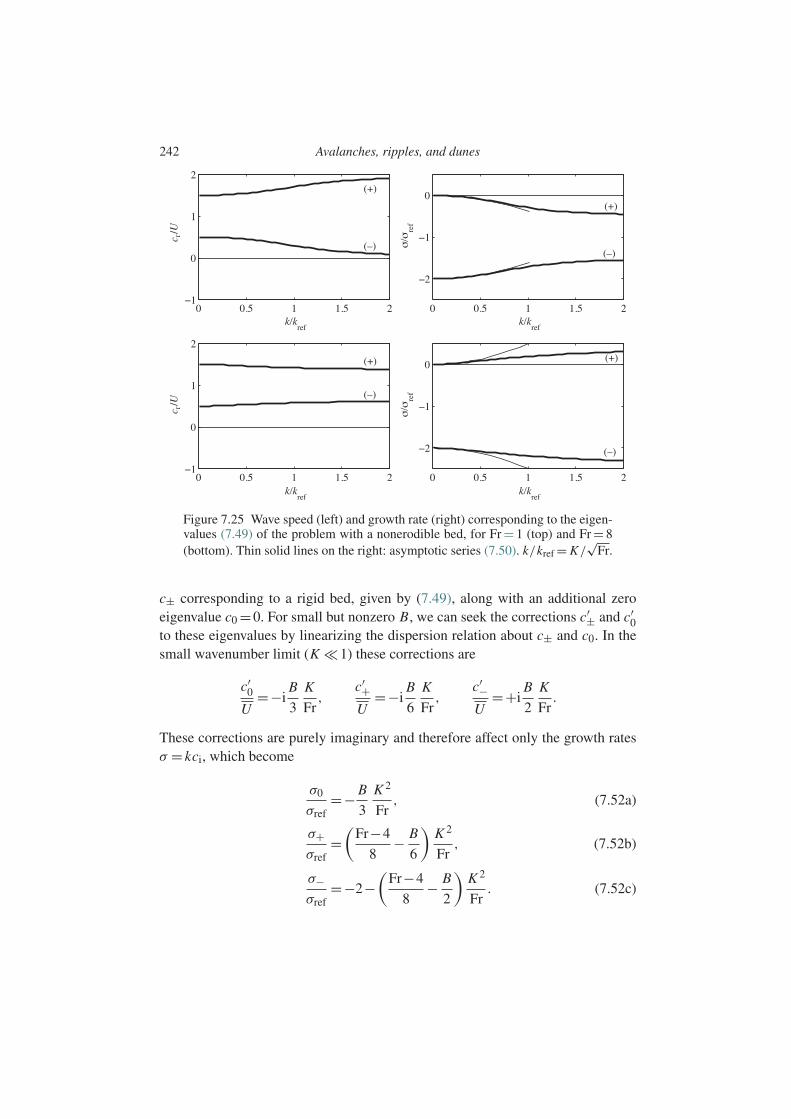
242 Avalanches, ripples, and dunes

c r/U

c r/U

(+)

(–)(–)

(+) (+)

(+)

(–)

(–)

Figure 7.25 Wave speed (left) and growth rate (right) corresponding to the eigen-values (7.49) of the problem with a nonerodible bed, for Fr = 1 (top) and Fr = 8(bottom). Thin solid lines on the right: asymptotic series (7.50). k/kref = K/

√Fr.

c± corresponding to a rigid bed, given by (7.49), along with an additional zeroeigenvalue c0 =0. For small but nonzero B, we can seek the corrections c′± and c′

0to these eigenvalues by linearizing the dispersion relation about c± and c0. In thesmall wavenumber limit (K 1) these corrections are

c′0

U=−i

B

3

K

Fr,

c′+U

=−iB

6

K

Fr,

c′−U

=+iB

2

K

Fr.

These corrections are purely imaginary and therefore affect only the growth ratesσ = kci, which become

σ0

σref=− B

3

K 2

Fr, (7.52a)

σ+σref

=(

Fr−4

8− B

6

)K 2

Fr, (7.52b)

σ−σref

=−2−(

Fr−4

8− B

2

)K 2

Fr. (7.52c)

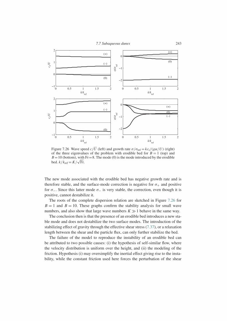
7.7 Subaqueous dunes 243c r

/Uc r

/U

(+)(+)

(+)(+)

(–)

(–)

(–)

(–)

(0)

(0)

(0)

(0)

Figure 7.26 Wave speed c/U (left) and growth rate σ/σref = kci/(gα/U ) (right)of the three eigenvalues of the problem with erodible bed for B = 1 (top) andB =10 (bottom), with Fr=8. The mode (0) is the mode introduced by the erodiblebed. k/kref = K/

√Fr.

The new mode associated with the erodible bed has negative growth rate and istherefore stable, and the surface-mode correction is negative for σ+ and positivefor σ−. Since this latter mode σ− is very stable, the correction, even though it ispositive, cannot destabilize it.

The roots of the complete dispersion relation are sketched in Figure 7.26 forB = 1 and B = 10. These graphs confirm the stability analysis for small wavenumbers, and also show that large wave numbers K 1 behave in the same way.

The conclusion then is that the presence of an erodible bed introduces a new sta-ble mode and does not destabilize the two surface modes. The introduction of thestabilizing effect of gravity through the effective shear stress (7.37), or a relaxationlength between the shear and the particle flux, can only further stabilize the bed.

The failure of the model to reproduce the instability of an erodible bed canbe attributed to two possible causes: (i) the hypothesis of self-similar flow, wherethe velocity distribution is uniform over the height, and (ii) the modeling of thefriction. Hypothesis (i) may oversimplify the inertial effect giving rise to the insta-bility, while the constant friction used here forces the perturbation of the shear

244 Avalanches, ripples, and dunes

stress to be in phase with that of the velocity. However, our earlier study of ripplesshowed that a phase shift is in fact crucial. We can attempt to generate an instabilityby relaxing the hypothesis for the friction coefficient in various ways (see Exer-cise 7.8.4). However, these offer little hope of obtaining a good description of theinstability mechanism, which has its origins in subtle phase shifts. Only consistentdepth-averaged equations can properly account for this phase shift.

7.8 Exercises

7.8.1 Stability of an avalanche

Establish the dispersion relation (7.5) for perturbations of an avalanche flow overan inclined plane. Show that in the limit Fr 1, all disturbances are damped. Findthe critical Froude number Frc = (a/b)2.

7.8.2 Stability of a river flow over a flat bed

Consider the problem studied in Section 7.7.3 of the stability of a flow above anonerodible flat bed (Q(τ )= 0). Use u, η, and τ to denote small perturbations ofthe velocity, the water depth, and the wall shear corresponding to the base flow(7.46). Linearize Eqs (7.42) and (7.43), introduce normal modes of the type

u = 1

2u ei(kx−ωt)+c.c.

in the usual fashion, and show that the amplitudes of the perturbations satisfy thehomogeneous system

−iωη+ ik(U η+h u) =0,

−iωρh u + ikρhU u =−ikρghη− τ +ρgα η,

τ = cfρUu.

Derive the dispersion relation (7.48).

7.8.3 Dunes: constant friction coefficient

Consider the case of an erodible bed studied in Section 7.7.4. Derive the linearizedequations for small perturbations u, ηb, η, q, and τ of the base flow (7.46), intro-duce the normal modes, and show that the amplitudes of these normal modes

7.8 Exercises 245

satisfy the homogeneous algebraic system

−iωη+ ik(U η+h u)=0,

−iωρh u + ikρhU u =−ikρgh cosα(ηb + η)− τ +ρg sinα η,

τ = cfρUu,

q = Q′(τ )τ ,

−iωηb + ik q =0.

Show that the dispersion relation is given by Eq. (7.48) with the additional term(7.51).

7.8.4 Dunes: nonconstant friction coefficient

Repeat the preceding exercise with a nonconstant friction coefficient given by:

1. the Blasius law cf =0.316Re−1/4, Re=ρUh/µ;2. the Manning–Strickler law cf = 0.1(z0/h)1/3, where z0 is the roughness scale

of the bed and is of the order of the grain diameter.

8

Nonlinear dynamics of systems with fewdegrees of freedom

8.1 Introduction

According to the linear stability theory developed in the preceding chapters, a per-turbation of a base flow can be expressed as a sum of eigenmodes, each uncoupledfrom the other and written as

u(x, t)= 1

2

(A(t) f (x)+ A∗(t) f ∗(x)

). (8.1)

Here f (x) describes the spatial structure of the mode and A(t) describes its timeevolution, with the asterisk denoting complex conjugation. However, the predic-tions of the linear analysis, and indeed this representation, are valid only forperturbations of sufficiently small amplitude, when the nonlinearities of the prob-lem are effectively negligible. The object of a nonlinear stability study is to predictwhat happens beyond the initial period of growth when nonlinear effects becomeimportant. Unfortunately, there is no general theory of nonlinear effects analogousto the linear stability theory, which exploits the linearity of the underlying math-ematical problem. Various approaches have been developed, each permitting thestudy of certain classes of nonlinearities and/or classes of solutions. One of theseapproaches, known as weakly nonlinear analysis, is particularly important owingto its fairly general nature based on perturbation methods.

The basic idea of weakly nonlinear analysis is due to the Soviet physicistLev Landau (1944) (see Landau and Lifshitz, 1987, §26). Landau first notes thatfor a linearized problem governed by constant coefficient equations, the (com-plex) amplitude A(t) of an eigenmode grows exponentially as the solution of thedifferential equation

dA

dt=σ A, (8.2)

246

8.1 Introduction 247

where σ is the temporal growth rate. For small A this equation can be viewed asa Taylor series expansion of the growth rate dA/dt in powers of the amplitude,truncated at first order. Therefore, nonlinearities can be treated in a natural way byincluding higher-order terms, first quadratic A2, AA∗, A∗2, then cubic A3, A2 A∗,and so on. Analysis of the symmetries of the problem generally allows a largenumber of these terms to be eliminated. Let us consider the important case ofa problem invariant under time translation, that is, invariant under change of tto t0 + t (arbitrary time origin t0). Then, if A ∝ eiσ t is a solution, any functiontranslated by a phase φ of the form A ∝ ei(σ t+φ) must also be a solution.1 Theequation for A must therefore be invariant under rotations in the complex planeA → Aeiφ . None of the quadratic or quartic terms satisfies this invariance, and theonly cubic term satisfying it is |A|2 A. Therefore, up to terms of fifth order theamplitude is governed by the nonlinear equation

dA

dt=σ A−κ|A|2 A. (8.3)

This equation, called the Landau amplitude equation, involves a new coefficient κwhich, like σ and A, is a priori complex and is known as the Landau coefficient.As we will see, this coefficient can be determined by means of a perturbationexpansion for small but finite amplitude instabilities.

In hydrodynamics the nonlinearity determining the Landau constant κ gener-ally comes from the advective acceleration term, but it can also arise from theboundary conditions on a deformable interface, a nonlinear constitutive law, or acoupling to nonhydrodynamic phenomena such as thermal convection. The gen-eral method of finding the Landau coefficient is to seek the solution of the problemas a power series in the amplitude of the perturbation to the base solution. The pio-neers of this “weakly nonlinear approach” were Gor’kov (1957) and Malkus andVeronis (1958) for thermal convection and Stuart (1958, 1960) and Watson (1960)for parallel shear flows.2 It has been shown that the Rayleigh–Benard instabilityis supercritical: for the marginal mode, the real part of κ is positive and the non-linear cubic term saturates the instability (Koschmieder, 1993). The same occursfor another well-studied fundamental instability, the Couette–Taylor centrifugalinstability (Chossat and Iooss, 1994). On the other hand, the instability of planePoiseuille flow is subcritical: for the marginal mode (kch = 1.02 for Rec = 5772;see Chapter 5) the real part of κ is negative and the instability is not saturatedby the nonlinear cubic term. In such a case of a subcritical instability the Landauequation is of little help, and the calculation of the higher-order stabilizing terms

1 The heuristic derivation presented here is made more precise later in this chapter and in Chapter 11.2 In hydrodynamics the Landau equation is sometimes more correctly called the Stuart–Landau equation, and

the technique used to derive it, the Stuart–Watson expansion.

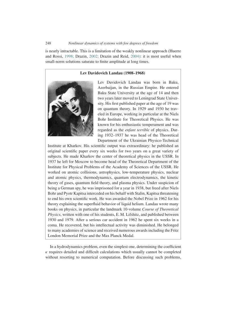
248 Nonlinear dynamics of systems with few degrees of freedom

is nearly intractable. This is a limitation of the weakly nonlinear approach (Huerreand Rossi, 1998; Drazin, 2002; Drazin and Reid, 2004): it is most useful whensmall-norm solutions saturate to finite amplitude at long times.

Lev Davidovich Landau (1908–1968)

Lev Davidovich Landau was born in Baku,Azerbaijan, in the Russian Empire. He enteredBaku State University at the age of 14 and thentwo years later moved to Leningrad State Univer-sity. His first published paper at the age of 19 wason quantum theory. In 1929 and 1930 he trav-eled in Europe, working in particular at the NielsBohr Institute for Theoretical Physics. He wasknown for his enthusiastic temperament and wasregarded as the enfant terrible of physics. Dur-ing 1932–1937 he was head of the TheoreticalDepartment of the Ukrainian Physico-Technical

Institute at Kharkov. His scientific output was extraordinary: he published anoriginal scientific paper every six weeks for two years on a great variety ofsubjects. He made Kharkov the center of theoretical physics in the USSR. In1937 he left for Moscow to become head of the Theoretical Department of theInstitute for Physical Problems of the Academy of Sciences of the USSR. Heworked on atomic collisions, astrophysics, low-temperature physics, nuclearand atomic physics, thermodynamics, quantum electrodynamics, the kinetictheory of gases, quantum field theory, and plasma physics. Under suspicion ofbeing a German spy, he was imprisoned for a year in 1938, but freed after NielsBohr and Pyotr Kapitsa interceded on his behalf with Stalin, Kapitsa threateningto end his own scientific work. He was awarded the Nobel Prize in 1962 for histheory explaining the superfluid behavior of liquid helium. Landau wrote manybooks on physics, in particular the landmark 10-volume Course of TheoreticalPhysics, written with one of his students, E. M. Lifshitz, and published between1930 and 1979. After a serious car accident in 1962 he spent six weeks in acoma. He recovered, but his intellectual activity was diminished. He belongedto many academies of science and received numerous awards including the FritzLondon Memorial Prize and the Max Planck Medal.

In a hydrodynamics problem, even the simplest one, determining the coefficientκ requires detailed and difficult calculations which usually cannot be completedwithout resorting to numerical computation. Before discussing such problems,

8.2 Nonlinear oscillators 249

it is instructive to consider simpler problems governed by ordinary differen-tial equations, especially the classical nonlinear oscillators. The first part of thischapter is devoted to analysis of these oscillators, using the techniques of per-turbation theory.3 With the help of the method of multiple scales, we show thatthe Landau equation can be obtained as a solvability condition of a differentialequation. Two important canonical nonlinear effects can be studied that are alsomanifested qualitatively in the same way in more complicated hydrodynamicsproblems: the saturation of the amplitude for the van der Pol oscillator, and theshift of the frequency for the Duffing oscillator. In the second part of the chapterwe return to spatio-temporal problems governed by partial differential equations.We show that when the spatial structure of the perturbation can be described by asmall number of Fourier modes, its dynamics can be described by a system of cou-pled equations for the amplitudes of the modes which reduces to a single Landauequation near the instability threshold.

In this chapter we focus on the “good” behaviors, periodic or quasi-periodic,which generally arise near the threshold of a primary instability and are accessi-ble to perturbation methods. Farther from the threshold, chaotic behavior occurs,whose analysis requires other techniques; see, for example, Berge et al. (1987).

8.2 Nonlinear oscillators

We begin by analyzing the simple classical problem of a particle in a potentialwell, which we mentioned briefly in the first chapter. This example will be usefulfor introducing the idea of saturation of an instability. Then we turn to the study ofnonlinear oscillators in order to gain a more general understanding of two majornonlinear effects. The first of these canonical effects is saturation of the exponen-tial growth at a finite value of the amplitude; the van der Pol oscillator (1927) isthe standard example of this. The second effect is the change of the oscillationfrequency, illustrated by the Duffing oscillator (1918). Forced oscillators are thenbriefly considered.

8.2.1 A strongly dissipative oscillator in a double-well potential

Let us consider an oscillator described by a real amplitude A(t) which evolvesin a potential V (A) assumed invariant under the reflection symmetry A −→ −A(V (A) is therefore an even function). In addition, we assume that this oscillator isstrongly dissipative, i.e., that the second-order “inertial” term d2 A/dt2 is negligiblecompared to a “friction force” proportional to dA/dt . This oscillator is therefore

3 Here we present only a basic introduction to a very rich topic; for further information see, for example,Bogolioubov and Mitropolski (1962) or Glendinning (1994, chapter 7).

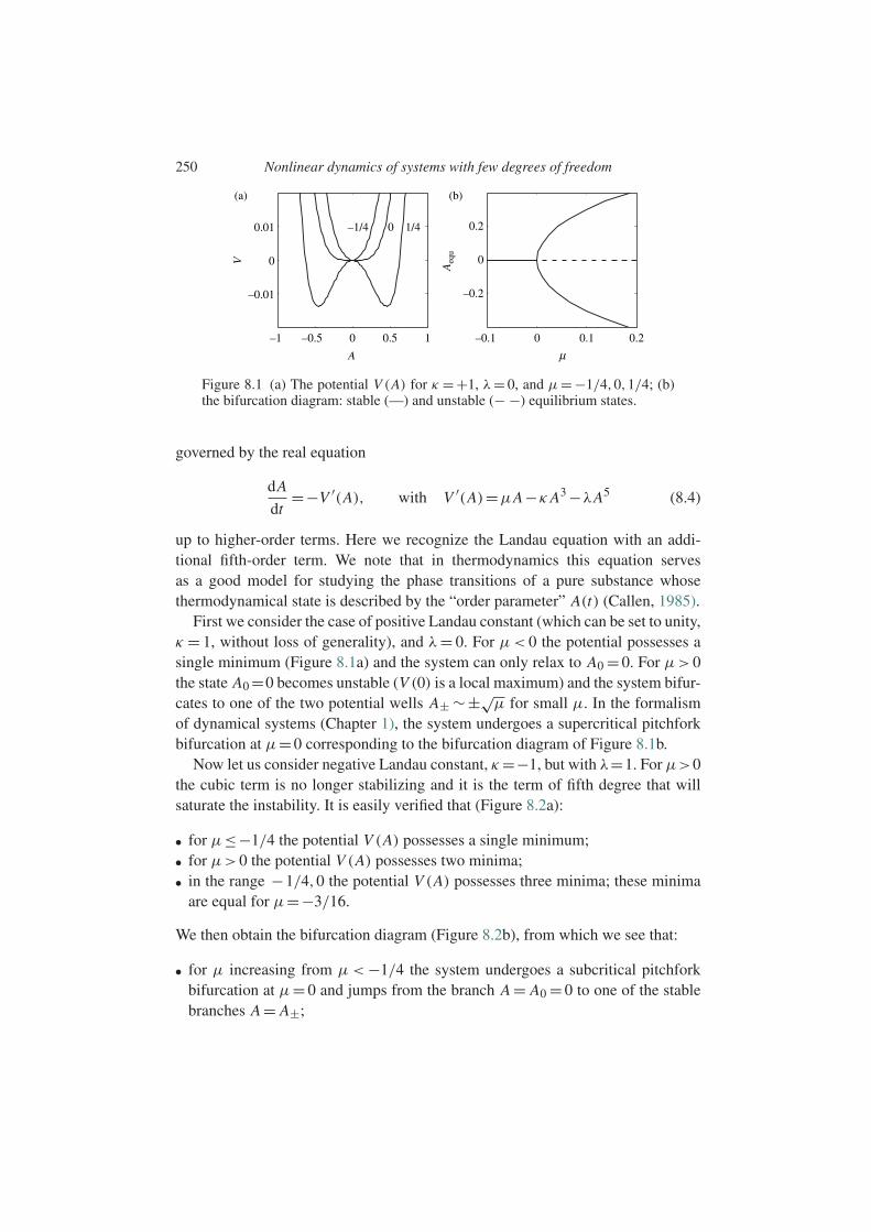
250 Nonlinear dynamics of systems with few degrees of freedom

–1 –0.5 0 0.5 1

–0.01

0

0.01

A

V

(a)

–1/4 0 1/4

–0.1 0 0.1 0.2

–0.2

0

0.2

µ

Aeq

u

(b)

Figure 8.1 (a) The potential V (A) for κ =+1, λ= 0, and µ=−1/4,0,1/4; (b)the bifurcation diagram: stable (—) and unstable (− −) equilibrium states.

governed by the real equation

dA

dt=−V ′(A), with V ′(A)=µA−κ A3 −λA5 (8.4)

up to higher-order terms. Here we recognize the Landau equation with an addi-tional fifth-order term. We note that in thermodynamics this equation servesas a good model for studying the phase transitions of a pure substance whosethermodynamical state is described by the “order parameter” A(t) (Callen, 1985).

First we consider the case of positive Landau constant (which can be set to unity,κ = 1, without loss of generality), and λ= 0. For µ< 0 the potential possesses asingle minimum (Figure 8.1a) and the system can only relax to A0 = 0. For µ> 0the state A0 =0 becomes unstable (V (0) is a local maximum) and the system bifur-cates to one of the two potential wells A± ∼±√

µ for small µ. In the formalismof dynamical systems (Chapter 1), the system undergoes a supercritical pitchforkbifurcation at µ=0 corresponding to the bifurcation diagram of Figure 8.1b.

Now let us consider negative Landau constant, κ=−1, but with λ=1. For µ>0the cubic term is no longer stabilizing and it is the term of fifth degree that willsaturate the instability. It is easily verified that (Figure 8.2a):

• for µ≤−1/4 the potential V (A) possesses a single minimum;• for µ>0 the potential V (A) possesses two minima;• in the range −1/4,0 the potential V (A) possesses three minima; these minima

are equal for µ=−3/16.

We then obtain the bifurcation diagram (Figure 8.2b), from which we see that:

• for µ increasing from µ< −1/4 the system undergoes a subcritical pitchforkbifurcation at µ= 0 and jumps from the branch A = A0 = 0 to one of the stablebranches A = A±;

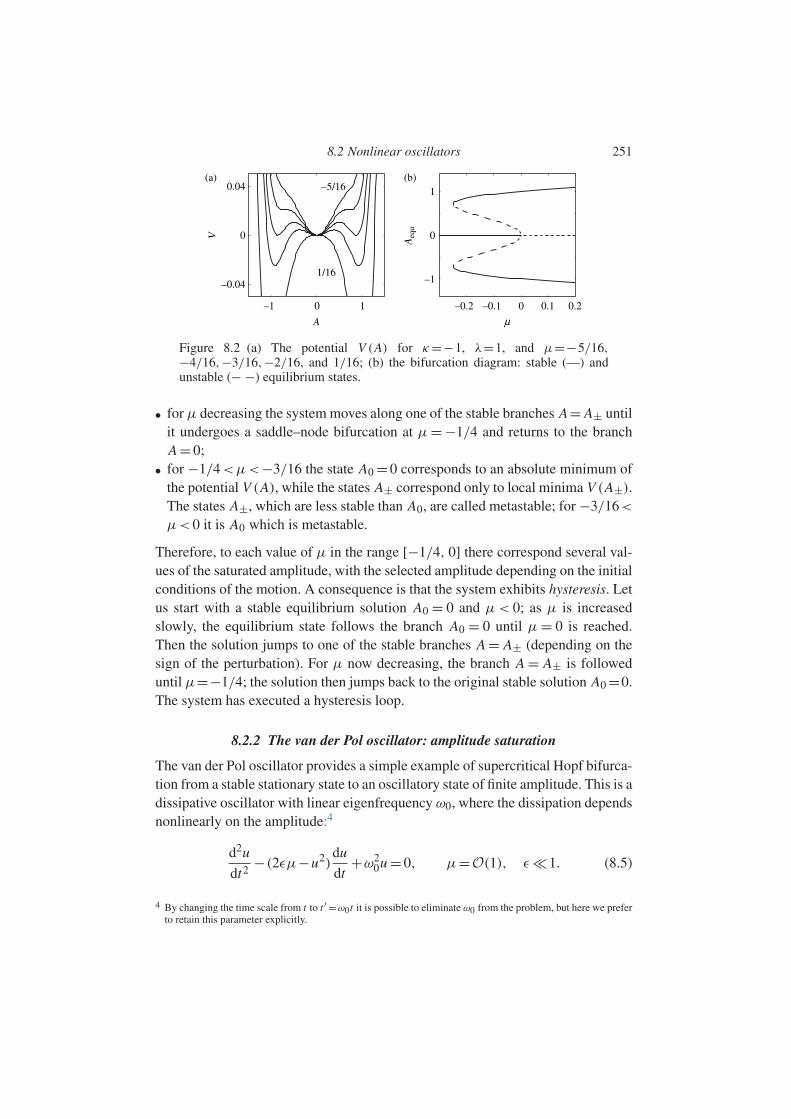
8.2 Nonlinear oscillators 251

–1 0 1

–0.04

0

0.04

A

V

(a)–5/16

1/16

–0.2 –0.1 0 0.1 0.2

–1

0

1

µ

Aeq

u

(b)

Figure 8.2 (a) The potential V (A) for κ=−1, λ=1, and µ=−5/16,−4/16,−3/16,−2/16, and 1/16; (b) the bifurcation diagram: stable (—) andunstable (− −) equilibrium states.

• for µ decreasing the system moves along one of the stable branches A= A± untilit undergoes a saddle–node bifurcation at µ= −1/4 and returns to the branchA =0;

• for −1/4<µ<−3/16 the state A0 =0 corresponds to an absolute minimum ofthe potential V (A), while the states A± correspond only to local minima V (A±).The states A±, which are less stable than A0, are called metastable; for −3/16<

µ<0 it is A0 which is metastable.

Therefore, to each value of µ in the range [−1/4, 0] there correspond several val-ues of the saturated amplitude, with the selected amplitude depending on the initialconditions of the motion. A consequence is that the system exhibits hysteresis. Letus start with a stable equilibrium solution A0 = 0 and µ< 0; as µ is increasedslowly, the equilibrium state follows the branch A0 = 0 until µ = 0 is reached.Then the solution jumps to one of the stable branches A = A± (depending on thesign of the perturbation). For µ now decreasing, the branch A = A± is followeduntil µ=−1/4; the solution then jumps back to the original stable solution A0 =0.The system has executed a hysteresis loop.

8.2.2 The van der Pol oscillator: amplitude saturation

The van der Pol oscillator provides a simple example of supercritical Hopf bifurca-tion from a stable stationary state to an oscillatory state of finite amplitude. This is adissipative oscillator with linear eigenfrequency ω0, where the dissipation dependsnonlinearly on the amplitude:4

d2u

dt2−(2εµ−u2)

du

dt+ω2

0u =0, µ=O(1), ε 1. (8.5)

4 By changing the time scale from t to t ′ =ω0t it is possible to eliminate ω0 from the problem, but here we preferto retain this parameter explicitly.

252 Nonlinear dynamics of systems with few degrees of freedom

We shall assume that the small parameter ε is fixed and that µ is the bifurcationparameter. It is easily verified5 that the solution u = 0 is linearly stable for µ< 0and unstable for µ> 0, that the frequency of small oscillations is ω0 +O(ε), andthat the growth rate is εµ, which is very small compared to ω0.

For µ>0, Eq. (8.5) shows that the term responsible for the instability vanishesfor u2 = 2εµ, so that we expect saturation for an amplitude of order ε1/2. Wetherefore seek a solution of the form

u(t)= ε1/2u(t), u =O(1), (8.6)

which leads to the following equation for u(t):

d2u

dt2−ε(2µ− u2)

du

dt+ω2

0u =0, µ=O(1), ε 1.

Since the growth rate of the linear instability is of order ε, we expect nonlineareffects to appear after a time of order ε−1, which is much larger than the oscil-lation period. We therefore seek an equation describing the slow variation of theamplitude of u(t) using the method of multiple scales (Bender and Orszag, 1978;Hinch, 1991; Glendinning, 1994). We set

u(t)= u(τ,T ), (8.7)

where τ = t is the “fast” time describing the phase variation and T = εt is the“slow” time describing the amplitude variation. Saturation is therefore expectedfor T =O(1). Next we seek u(τ,T ) as a series in powers of ε:

u =u0 +εu1 +ε2u2 + ... (8.8)

Using the rule for the derivative of a composite function,

d

dt= ∂

∂τ+ε

∂

∂T,

substituting into the original equation and collecting terms of the same order in ε,we obtain the series of differential equations. At orders ε0 and ε1 these equations

5 Within the framework of the theory of dynamical systems (Chapter 1), the van der Pol equation can be writtenas a system of ordinary differential equations of first order in u and v=du/dt , whose solutions are representedby curves in the phase space (u,v). The eigenvalues of the linearized system are complex conjugates of eachother and the fixed point (u,v)= (0,0) is a focus. For µ<0 (µ>0) this focus is stable (unstable) and the phaseportrait in its vicinity consists of convergent (divergent) spirals. For µ= 0 the fixed point is a center, and thephase portrait of the linearized system consists of closed ellipses.

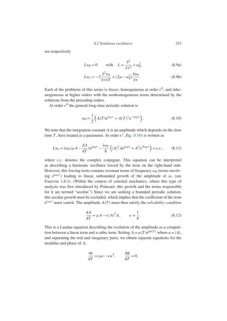
8.2 Nonlinear oscillators 253

are respectively

Lu0 =0 with L = ∂2

∂τ 2+ω2

0, (8.9a)

Lu1 =−2∂2u0

∂τ∂T+(2µ−u2

0)∂u0

∂τ. (8.9b)

Each of the problems of this series is linear, homogeneous at order ε0, and inho-mogeneous at higher orders with the nonhomogeneous terms determined by thesolutions from the preceding orders.

At order ε0 the general long-time periodic solution is

u0 = 1

2

(A(T )eiω0τ + A(T )∗e−iω0τ

). (8.10)

We note that the integration constant A is an amplitude which depends on the slowtime T , here treated as a parameter. At order ε1, Eq. (8.9b) is written as

Lu1 = iω0 (µA− dA

dT)eiω0τ − iω0

8

(|A|2 Aeiω0τ + A3e3iω0τ

)+c.c., (8.11)

where c.c. denotes the complex conjugate. This equation can be interpretedas describing a harmonic oscillator forced by the term on the right-hand side.However, this forcing term contains resonant terms of frequency ω0 (terms involv-ing eiω0τ ) leading to linear, unbounded growth of the amplitude of u1 (seeExercise 1.6.1). (Within the context of celestial mechanics, where this type ofanalysis was first introduced by Poincare, this growth and the terms responsiblefor it are termed “secular.”) Since we are seeking a bounded periodic solution,this secular growth must be excluded, which implies that the coefficient of the termeiω0τ must vanish. The amplitude A(T ) must then satisfy the solvability condition

dA

dT=µA−κ|A|2 A, κ = 1

8. (8.12)

This is a Landau equation describing the evolution of the amplitude as a competi-tion between a linear term and a cubic term. Setting A=a(T )eiφ(T ) where a =|A|,and separating the real and imaginary parts, we obtain separate equations for themodulus and phase of A:

da

dT=µa −κa3,

dφ

dT=0.

254 Nonlinear dynamics of systems with few degrees of freedom

0.5

2

0

–2

uu

(a)

(b)

0

–0.5

0 5 10 15 20

0 5 10

ω0t/2π15 20

Figure 8.3 Response of the van der Pol oscillator (8.5) for the initial conditionsu(0) = 0.02, u′(0) = 0: (a) 2εµ = 0.1, (b) 2εµ = 1. For the sake of clarity theasymptotic solution (8.14) is represented only by its amplitude (8.13), and theoscillating curve corresponds to the numerical solution.

For µ positive the solutions of these equations are

a =a0

(κ

µa2

0 +(1− κ

µa2

0)e−2µT

)−1/2

, (8.13a)

φ=φ0, (8.13b)

from which we finally obtain the solution for u(t):

u(t)= ε1/2a(t)cos(ω0t +φ0)+O(ε3/2). (8.14)

This result, which conforms to the initial conjecture u(t)∼ ε1/2, shows that theamplitude of the saturated oscillation is 2

√2µε and its frequency is ω0, indepen-

dent of the amplitude of the order to which we are working. Figure 8.3 comparesthe numerical solution of Eq. (8.5) to the asymptotic solution (8.14), representedonly by its envelope a(t), for two values of 2µε. The agreement is excellentnot only near threshold (2µε = 0.1, Figure 8.3a), but also relatively far from it(2µε = 1, Figure 8.3b). However, we see that for 2µε = 1 the numerical solu-tion is not quite sinusoidal, which corresponds to the presence of harmonics ofthe fundamental frequency ω0/2π . These harmonics do not exist in the asymp-totic solution (8.14), but they can be determined by pursuing the calculations tohigher order. Figure 8.4 shows the corresponding phase portraits for the numeri-cal solution. Close to threshold (2εµ= 0.1, left-hand portrait) the limit cycle is acircle, which corresponds to a sinusoidal response. Far from threshold (2εµ= 1,

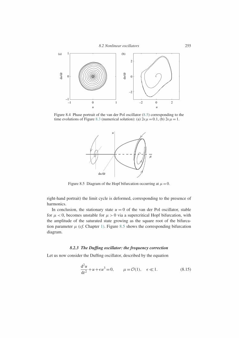
8.2 Nonlinear oscillators 255

1

0

(a) (b)

2

0

–2

–1–1

du/d

t

du/d

t

0 1 –2 0 2

u u

Figure 8.4 Phase portrait of the van der Pol oscillator (8.5) corresponding to thetime evolutions of Figure 8.3 (numerical solution): (a) 2εµ=0.1, (b) 2εµ=1.

u

du/dt

µ

Figure 8.5 Diagram of the Hopf bifurcation occurring at µ=0.

right-hand portrait) the limit cycle is deformed, corresponding to the presence ofharmonics.

In conclusion, the stationary state u = 0 of the van der Pol oscillator, stablefor µ< 0, becomes unstable for µ> 0 via a supercritical Hopf bifurcation, withthe amplitude of the saturated state growing as the square root of the bifurca-tion parameter µ (cf. Chapter 1). Figure 8.5 shows the corresponding bifurcationdiagram.

8.2.3 The Duffing oscillator: the frequency correction

Let us now consider the Duffing oscillator, described by the equation

d2u

dt2+u +εu3 =0, µ=O(1), ε 1. (8.15)

256 Nonlinear dynamics of systems with few degrees of freedom

15

10

5V

0

–5–5

ε = 0.1

ε = –0.1

0 5

u

Figure 8.6 (a) The potential V (u) for ε = −0.1 (− −), ε = 0 (—), and ε = 0.1(−·−).

This equation can also be written as

d2u

dt2=−V ′(u), V (u)= u2

2+ε

u4

4,

which we recognize as the equation of motion of a mass with a single degreeof freedom u(t), subject to a force F = −V ′(u) deriving from a potential V (u),with the scales chosen such that the mass and eigenfrequency of the oscillator arenormalized to unity. For example, for a simple pendulum in a gravity field thedegree of freedom is the angular position, and the restoring force F =−sinu maybe approximated by F =−u +u3/6 for small u, which corresponds to ε =−1/6.The potential V (u) is shown in Figure 8.6 for three values of the parameter ε.

The Duffing equation admits the first integral

H(u,v)= H0, where H(u,v)= 1

2v2 +V (u) (8.16)

with v=du/dt , which represents the constant mechanical energy of the oscillator.The energy curves H(u,v)= constant define trajectories in the phase space (u,v),which are ellipses centered on the fixed point (0,0).6 The corresponding peri-odic solution u(t) can be found by a perturbation method leading to an amplitudeequation.

We seek the solution in the form of a series in powers of ε

u(t)=u0(t)+εu1(t)+ ...,

and introduce a fast time τ = t and a slow time T = εt . We then have a hierarchyof linear equations, similar to the van der Pol oscillator. At orders ε0 and ε1 these

6 For ε<0 there exist two other fixed points (±(−ε)−1/2,0), which are saddles. These saddles are joined by twoheteroclinic trajectories outside which the trajectories are unbounded.

8.2 Nonlinear oscillators 257

equations are respectively

Lu0 =0 with L = ∂2

∂τ 2+1, (8.17a)

Lu1 =−2∂2u0

∂τ∂T−u3

0. (8.17b)

At order ε0 the solution corresponds to harmonic oscillations, as for the van derPol oscillator. At order ε1 the equation to be solved is

Lu1 =(−i

dA

dT− 3

8|A|2 A

)eiτ − 1

8A3e3iτ +c.c.

This equation can be interpreted as that of a forced harmonic oscillator, whoseresponse can be periodic only if the coefficient of the resonant forcing on the right-hand side is zero. Hence the solvability condition gives

dA

dT= 3i

8|A|2 A. (8.18)

We therefore recover a Landau equation with no linear term (zero linear growthrate) and purely imaginary Landau coefficient of the cubic term, κ=−3i/2. SettingA = a(T )eiφ(T ) and separating the real and imaginary parts of this equation, weobtain

da

dT=0,

dφ

dT= 3

8a2. (8.19)

The solutions of these equations are

a =a0, φ= 3

8a2

0 T +φ0, (8.20)

which leads to the expression for u(t):

u(t)=a0 cos(ωt +φ0)+O(ε), ω=1+ 3

8εa2

0 +O(ε2). (8.21)

Therefore, the nonlinear term of the Duffing equation does not affect the oscil-lation amplitude but only the frequency, in contrast to the case of the van der Poloscillator.7 The frequency correction of order εa2

0 can be interpreted by treating

7 If we had defined the potential without a small parameter and looked for a small solution of order ε, wewould have found the frequency correction 3

8 ε2a2

0 , of order ε2. The difference arises solely from the differentdefinition of the small parameter.

258 Nonlinear dynamics of systems with few degrees of freedom

1

0

–10 2 4 6 8 10 12

t/2π

u

Figure 8.7 Response of the Duffing oscillator (8.15) for ε = 0.3: (—) numericalsolution, (− −) solution at order ε0, (−·−) solution at order ε1 (8.21).

the Duffing equation (8.15) as the equation for an oscillator subject to a restoringforce

F =−(1+εu2)u ≈−(1+εa20)u.

This force corresponds to that of a nonlinear spring with stiffness r = 1 + εa20

depending on the oscillation amplitude a0. The corresponding frequency is thenω = r1/2 ≈ 1+ 1

2εa20, which clearly depends on the amplitude following a law of

the same type as (8.21).Figure 8.7 presents a comparison of the solutions at orders ε0 and ε1 with the

exact solution obtained numerically. As expected, we see that the order ε0 solutionis valid only for t 1/ε and the order ε1 one for t 1/ε2, i.e., as long as the(uncalculated) phase correction remains small. For t of order 1/ε2 the order ε2

correction should be included, see Hinch (1991, §6.2). See Guckenheimer andHolmes (1983, §2.2) for a detailed study of the Duffing oscillator.

8.2.4 Forced oscillators

The forcing of a nonlinear oscillator leads to remarkable and unexpected phenom-ena. Here we give a brief discussion of a few of them for the two cases of the vander Pol oscillator and parametrically forced oscillators, leaving the calculationsand the study of frequency locking phenomena as exercises. For more details thereader may consult one of the many expositions on the subject, for example thoseof Bender and Orszag (1978) and Glendinning (1984).

The forced van der Pol oscillator

We consider the van der Pol oscillator (8.5) subject to a forcing of frequency ωf

and amplitude F , described by the equation

d2u

dt2−(2εµ−u2)

du

dt+ω2

0u = F cosωft, 0<ε 1, (8.22)

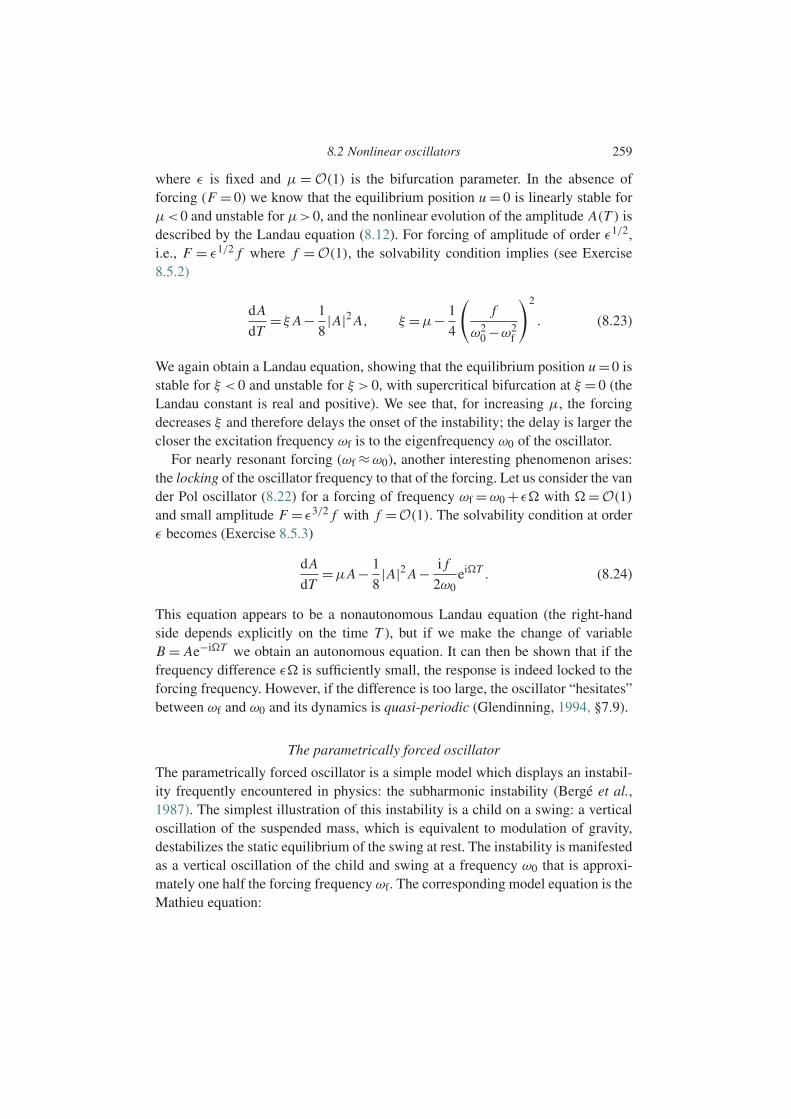
8.2 Nonlinear oscillators 259

where ε is fixed and µ = O(1) is the bifurcation parameter. In the absence offorcing (F = 0) we know that the equilibrium position u = 0 is linearly stable forµ<0 and unstable for µ>0, and the nonlinear evolution of the amplitude A(T ) isdescribed by the Landau equation (8.12). For forcing of amplitude of order ε1/2,i.e., F = ε1/2 f where f =O(1), the solvability condition implies (see Exercise8.5.2)

dA

dT= ξ A− 1

8|A|2 A, ξ =µ− 1

4

(f

ω20 −ω2

f

)2

. (8.23)

We again obtain a Landau equation, showing that the equilibrium position u =0 isstable for ξ < 0 and unstable for ξ > 0, with supercritical bifurcation at ξ = 0 (theLandau constant is real and positive). We see that, for increasing µ, the forcingdecreases ξ and therefore delays the onset of the instability; the delay is larger thecloser the excitation frequency ωf is to the eigenfrequency ω0 of the oscillator.

For nearly resonant forcing (ωf ≈ω0), another interesting phenomenon arises:the locking of the oscillator frequency to that of the forcing. Let us consider the vander Pol oscillator (8.22) for a forcing of frequency ωf =ω0 + ε with =O(1)and small amplitude F = ε3/2 f with f =O(1). The solvability condition at orderε becomes (Exercise 8.5.3)

dA

dT=µA− 1

8|A|2 A− i f

2ω0eiT . (8.24)

This equation appears to be a nonautonomous Landau equation (the right-handside depends explicitly on the time T ), but if we make the change of variableB = Ae−iT we obtain an autonomous equation. It can then be shown that if thefrequency difference ε is sufficiently small, the response is indeed locked to theforcing frequency. However, if the difference is too large, the oscillator “hesitates”between ωf and ω0 and its dynamics is quasi-periodic (Glendinning, 1994, §7.9).

The parametrically forced oscillator

The parametrically forced oscillator is a simple model which displays an instabil-ity frequently encountered in physics: the subharmonic instability (Berge et al.,1987). The simplest illustration of this instability is a child on a swing: a verticaloscillation of the suspended mass, which is equivalent to modulation of gravity,destabilizes the static equilibrium of the swing at rest. The instability is manifestedas a vertical oscillation of the child and swing at a frequency ω0 that is approxi-mately one half the forcing frequency ωf. The corresponding model equation is theMathieu equation:

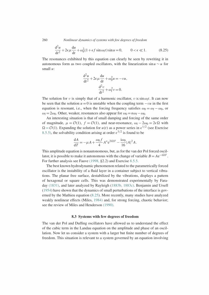
260 Nonlinear dynamics of systems with few degrees of freedom

d2u

dt2+2εµ

du

dt+ω2

0(1+ε f sinωft)sinu =0, 0<ε 1. (8.25)

The resonances exhibited by this equation can clearly be seen by rewriting it inautonomous form as two coupled oscillators, with the linearization sinu ∼ u forsmall u:

d2u

dt2+2εµ

du

dt+ω2

0u =−vu,

d2v

dt2+ω2

f v=0.

The solution for v is simply that of a harmonic oscillator, v∝ sinωft . It can nowbe seen that the solution u =0 is unstable when the coupling term −vu in the firstequation is resonant, i.e., when the forcing frequency satisfies ω0 = ωf −ω0, orωf =2ω0. Other, weaker, resonances also appear for ω0 =nωf −ω0.

An interesting situation is that of small damping and forcing of the same orderof magnitude, µ = O(1), f = O(1), and near-resonance, ωf − 2ω0 = 2ε with=O(1). Expanding the solution for u(t) as a power series in ε1/2 (see Exercise8.5.5), the solvability condition arising at order ε3/2 is found to be

dA

dT=−µA+ ω0 f

4A∗e2iT − iω0

16|A|2 A.

This amplitude equation is nonautonomous, but, as for the van der Pol forced oscil-lator, it is possible to make it autonomous with the change of variable B = Ae−iT .For further analysis see Fauve (1998, §2.2) and Exercise 8.5.5.

The best known hydrodynamic phenomenon related to the parametrically forcedoscillator is the instability of a fluid layer in a container subject to vertical vibra-tions. The planar free surface, destabilized by the vibrations, displays a patternof hexagonal or square cells. This was demonstrated experimentally by Fara-day (1831), and later analyzed by Rayleigh (1883b, 1883c). Benjamin and Ursell(1954) have shown that the dynamics of small perturbations of the interface is gov-erned by the Mathieu equation (8.25). More recently, many studies have analyzedweakly nonlinear effects (Miles, 1984) and, for strong forcing, chaotic behavior;see the review of Miles and Henderson (1990).

8.3 Systems with few degrees of freedom

The van der Pol and Duffing oscillators have allowed us to understand the effectof the cubic term in the Landau equation on the amplitude and phase of an oscil-lation. Now let us consider a system with a larger but finite number of degrees offreedom. This situation is relevant to a system governed by an equation involving

8.3 Systems with few degrees of freedom 261

partial derivatives with respect to time and space, where the smallest possible wavenumber is imposed by the finite size of the system or by a periodicity condition andwhere, at the other end of the wave number spectrum, a dissipative process at smallscales limits the number of Fourier components.

8.3.1 A model equation

Let us consider the Kuramoto–Sivashinsky (KS) model equation:

∂t u +2V u∂x u + R∂xx u + S∂xxxx u =0. (8.26)

This equation describes, for example, the height of the free surface of a thin filmfalling down an inclined plane, the position of a flame front, or the concentrationof chemical species in a reactive system (Cross and Hohenberg, 1993). For S = 0it becomes the Burgers equation, an elementary model which describes competingadvection and diffusion. For S >0 (the most common case), the fourth-order termcorresponds to a dissipative process at small scales, such as surface tension in thecase of the falling film.8

The essential features of the dynamics of a system with a small number ofdegrees of freedom can be illustrated by seeking solutions of the KS equationwhose spatial structure involves a finite number N of Fourier components:

u(x, t)= 1

2

N∑n=−N

An(t)eink1x , with A−n = A∗

n. (8.27)

Here the term “degree of freedom” refers to the complex amplitudes An(t) of theFourier components, and the term “small” means “finite” in principle and often“two or three” in practice. We shall see that study of the spatially periodic solu-tions of the KS equation displays the essential role played by the harmonics in thenonlinear evolution of an unstable fundamental mode, and allows interpretation ofmany results obtained experimentally and/or by numerical simulation.

8.3.2 The amplitude equations

Equation (8.26) admits the solution u0 = 0. Linearizing the equation for perturba-tions of this base solution and seeking these perturbations in the form of normalmodes proportional to eσ t+i(ωt−kx), we obtain the dispersion relation

σ + iω= Rk2 − Sk4. (8.28)

8 A slightly different equation, ∂t u − sinu − R∂xx u = 0, is studied in the same spirit by Drazin and Reid (2004,§50) and Drazin (2002, §5.2), while another, ∂t u +u∂x u = Ru − (∂xx +1)2u, is studied by Manneville (1990,chapter 5).

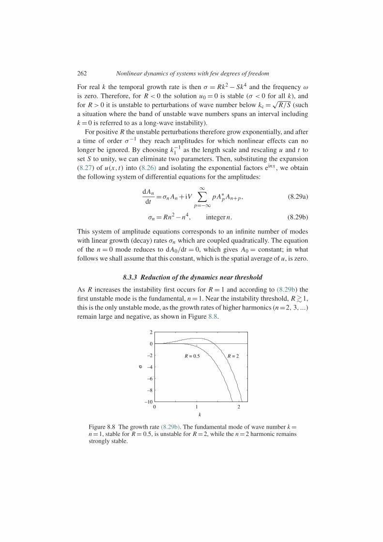
262 Nonlinear dynamics of systems with few degrees of freedom

For real k the temporal growth rate is then σ = Rk2 − Sk4 and the frequency ω

is zero. Therefore, for R < 0 the solution u0 = 0 is stable (σ < 0 for all k), andfor R > 0 it is unstable to perturbations of wave number below kc =√

R/S (sucha situation where the band of unstable wave numbers spans an interval includingk =0 is referred to as a long-wave instability).

For positive R the unstable perturbations therefore grow exponentially, and aftera time of order σ−1 they reach amplitudes for which nonlinear effects can nolonger be ignored. By choosing k−1

1 as the length scale and rescaling u and t toset S to unity, we can eliminate two parameters. Then, substituting the expansion(8.27) of u(x, t) into (8.26) and isolating the exponential factors einx , we obtainthe following system of differential equations for the amplitudes:

dAn

dt=σn An + iV

∞∑p=−∞

p A∗p An+p, (8.29a)

σn = Rn2 −n4, integer n. (8.29b)

This system of amplitude equations corresponds to an infinite number of modeswith linear growth (decay) rates σn which are coupled quadratically. The equationof the n = 0 mode reduces to dA0/dt = 0, which gives A0 = constant; in whatfollows we shall assume that this constant, which is the spatial average of u, is zero.

8.3.3 Reduction of the dynamics near threshold

As R increases the instability first occurs for R = 1 and according to (8.29b) thefirst unstable mode is the fundamental, n =1. Near the instability threshold, R1,this is the only unstable mode, as the growth rates of higher harmonics (n=2, 3, ...)remain large and negative, as shown in Figure 8.8.

0 1 2–10

–8

–6

–4

–2

0

2

R = 0.5 R = 2

k

σ

Figure 8.8 The growth rate (8.29b). The fundamental mode of wave number k =n =1, stable for R = 0.5, is unstable for R =2, while the n =2 harmonic remainsstrongly stable.

8.3 Systems with few degrees of freedom 263

Thus, for R1, we expect the amplitude of the perturbation to remain small, oforder ε 1, and to be dominated by the fundamental mode. Let us assume, to beconfirmed later, that the amplitude of the nth harmonic is of order εn . Then, keep-ing the first three harmonics, the system (8.29) reduces to the dynamical system

dA1

dt=σ1 A1 − iV A∗

1 A2 +O(A51), (8.30a)

dA2

dt=σ2 A2 − iV A2

1 +O(A41), (8.30b)

dA3

dt=σ3 A3 −3iV A1 A2 +O(A5

1). (8.30c)

This dynamical system can be simplified further near threshold. Indeed, for R 1 only the fundamental mode A1 is weakly unstable while the other modes arestrongly damped, i.e.,

σ1 >0, σn <0 with |σn|σ1. (8.31)

This means that following a very short initial transient during which the effects ofinitial conditions die out (due to the strong damping), the evolution of the highermodes will be driven by the forcing from the nonlinear coupling terms on the right-hand sides of (8.30b), (8.30c), etc. The time scale for the growth of the unstablemode, A1, is the inverse growth rate σ−1

1 . This is also the time scale for the evo-lution of the higher-order modes, so that the variation rate of all harmonics is, inorder of magnitude,

dAn

dt∼σ1 An. (8.32)

Since σ1 |σn| for n ≥ 2, we deduce that the variation rate of the harmonics in(8.30b) and (8.30c), dA2/dt and dA3/dt , is much smaller than σ2 A2 and σ3 A3,respectively. Therefore, the amplitudes A2 and A3 are given by the quasi-staticbalance of the terms on the right-hand sides:

A2 = iV

σ2A2

1 +O(A41), (8.33a)

A3 = 3iV

σ3A1 A2 +O(A5

1)∼− 3V 2

σ2σ3A3

1. (8.33b)

We note that for A1 ∼ ε we do in fact have An ∼ εn , which conforms to the initialassumption. Substituting the above expression for A2 into (8.30a), we find that the

264 Nonlinear dynamics of systems with few degrees of freedom

dynamics of the fundamental is governed by the Landau equation:

dA1

dt=σ1 A1 −κ|A1|2 A1 +O(A5

1), κ =−V 2

σ2, (8.34)

where the Landau constant κ is real and positive (because σ2 < 0). Let us checkthe orders of magnitude. Letting ε2 = R −1 be the distance from threshold, from(8.29) we have σ1 = ε2, and the saturated amplitude for A1 at long times is indeedof order ε. For times of order σ−1

1 all the terms of the Landau equation (8.34) arethen of the same order, ε3.

Setting An(t) = an(t)eiφn(t) and separating the real and imaginary parts, weobtain

da1

dt=σ1a1 −κa3

1,dφ1

dt=0. (8.35)

We recognize the equation for a1 as the normal form of the pitchfork bifurcationat σ1 =0 (R =1), and that it is supercritical because κ is positive.

Therefore, near the instability threshold (R = 1) the weakly nonlinear dynam-ics of the fundamental mode is governed by a Landau equation. The dynamicsof higher-order harmonics is “slaved” to that of the fundamental mode throughEqs (8.33a)–(8.33b); although these harmonics are linearly stable and stronglydamped (σn < 0), they become finite via the weak nonlinear interaction with thefundamental mode; it is this coupling that forces the amplitude of the highermodes and “pumps” energy into them and out of the fundamental, thus leadingto saturation of the instability.

The theory of dynamical systems allows the above process of reduction to thedynamics of the marginal mode to be made systematic; this systematization con-sists of projecting the equations of the perturbation onto a subspace of the spacespanned by the amplitudes (the degrees of freedom), the so-called “central mani-fold.” This approach is developed in Chapter 11, as well as by Glendinning (1994),Manneville (1990, chapter 5), and Newell et al. (1993).

8.4 Illustration: instability of a sheared interface

The above general results are illustrated here with an experimental study of theinstability of a sheared interface between two viscous fluids (Barthelet et al., 1995).The experimental setup, shown schematically in Figure 8.9, consists of an annularchannel of rectangular cross-section partially filled with a first liquid above whichlies a second, less dense liquid (a water–glycerin mixture and a mineral oil). Thechannel is enclosed by an upper plate whose rotation drags the fluids, and theposition of the interface is measured by conductance probes. The vertical velocity

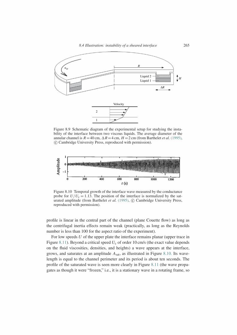
8.4 Illustration: instability of a sheared interface 265

∆R

HLiquid 2

2

1

Velocity

uω

Liquid 1

R

Figure 8.9 Schematic diagram of the experimental setup for studying the insta-bility of the interface between two viscous liquids. The average diameter of theannular channel is R =40 cm, R =4 cm, H =2 cm (from Barthelet et al. (1995),c© Cambridge University Press, reproduced with permission).

Figure 8.10 Temporal growth of the interface wave measured by the conductanceprobe for U/Uc = 1.13. The position of the interface is normalized by the sat-urated amplitude (from Barthelet et al. (1995), c© Cambridge University Press,reproduced with permission).

profile is linear in the central part of the channel (plane Couette flow) as long asthe centrifugal inertia effects remain weak (practically, as long as the Reynoldsnumber is less than 100 for the aspect ratio of the experiment).

For low speeds U of the upper plate the interface remains planar (upper trace inFigure 8.11). Beyond a critical speed Uc of order 10 cm/s (the exact value dependson the fluid viscosities, densities, and heights) a wave appears at the interface,grows, and saturates at an amplitude Asat, as illustrated in Figure 8.10. Its wave-length is equal to the channel perimeter and its period is about ten seconds. Theprofile of the saturated wave is seen more clearly in Figure 8.11 (the wave propa-gates as though it were “frozen,” i.e., it is a stationary wave in a rotating frame, so

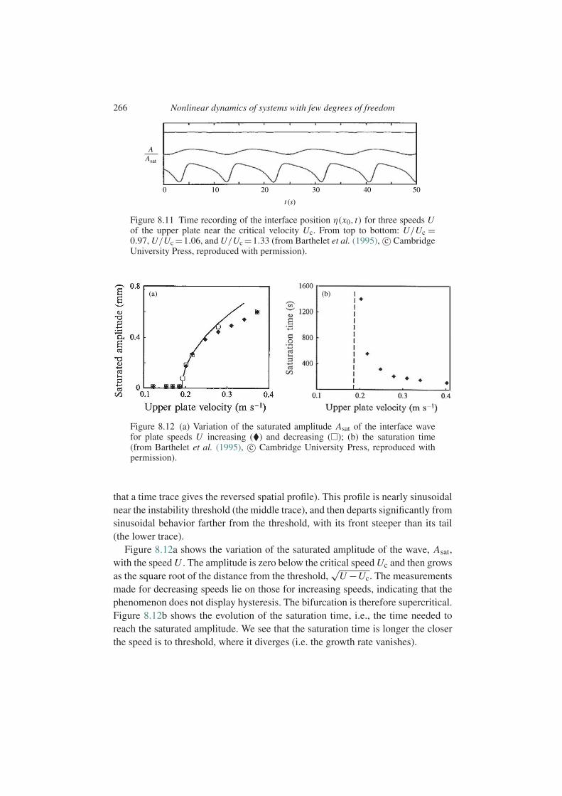
266 Nonlinear dynamics of systems with few degrees of freedom

20 30

t (s)

40 50100

Asat

A

Figure 8.11 Time recording of the interface position η(x0, t) for three speeds Uof the upper plate near the critical velocity Uc. From top to bottom: U/Uc =0.97, U/Uc =1.06, and U/Uc =1.33 (from Barthelet et al. (1995), c© CambridgeUniversity Press, reproduced with permission).

(a) (b)

Figure 8.12 (a) Variation of the saturated amplitude Asat of the interface wavefor plate speeds U increasing () and decreasing (); (b) the saturation time(from Barthelet et al. (1995), c© Cambridge University Press, reproduced withpermission).

that a time trace gives the reversed spatial profile). This profile is nearly sinusoidalnear the instability threshold (the middle trace), and then departs significantly fromsinusoidal behavior farther from the threshold, with its front steeper than its tail(the lower trace).

Figure 8.12a shows the variation of the saturated amplitude of the wave, Asat,with the speed U . The amplitude is zero below the critical speed Uc and then growsas the square root of the distance from the threshold,

√U −Uc. The measurements

made for decreasing speeds lie on those for increasing speeds, indicating that thephenomenon does not display hysteresis. The bifurcation is therefore supercritical.Figure 8.12b shows the evolution of the saturation time, i.e., the time needed toreach the saturated amplitude. We see that the saturation time is longer the closerthe speed is to threshold, where it diverges (i.e. the growth rate vanishes).

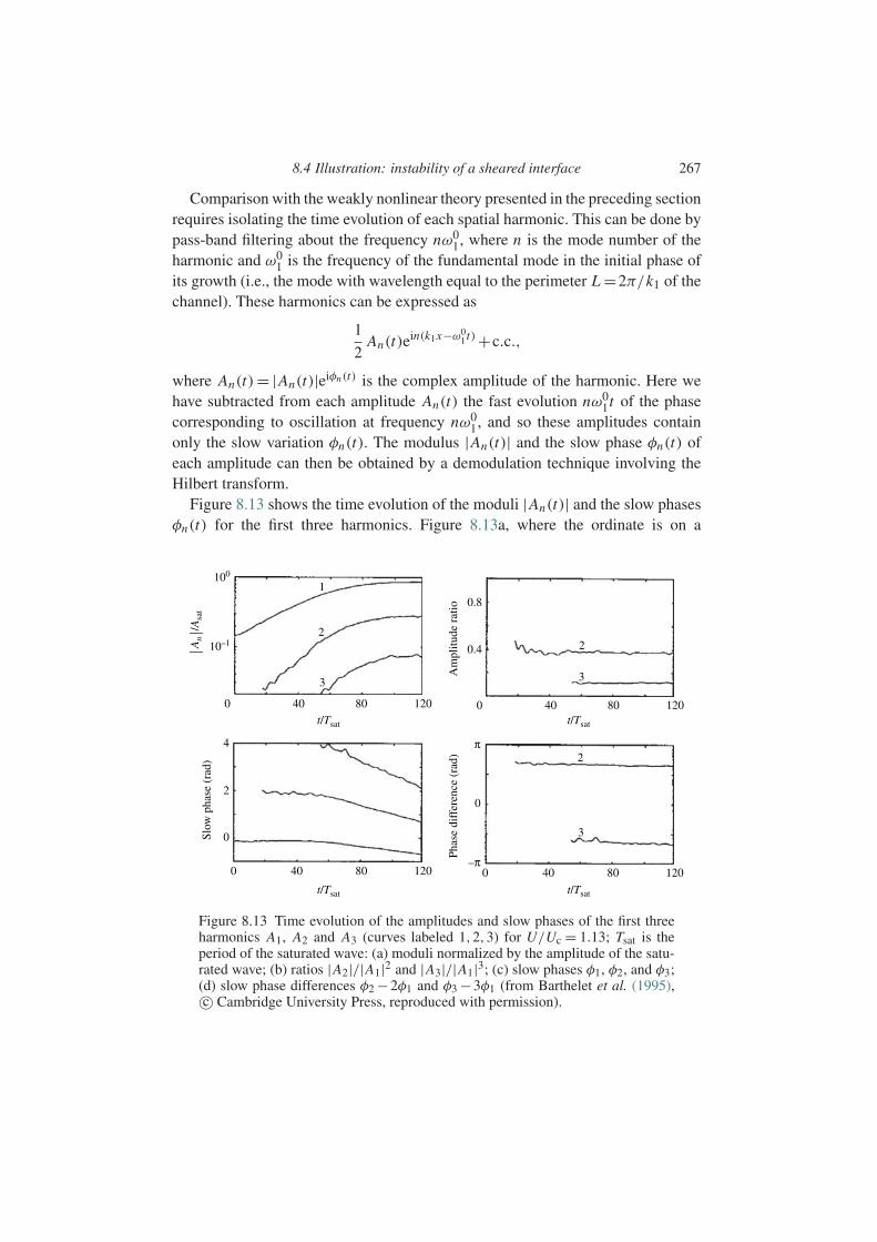
8.4 Illustration: instability of a sheared interface 267

Comparison with the weakly nonlinear theory presented in the preceding sectionrequires isolating the time evolution of each spatial harmonic. This can be done bypass-band filtering about the frequency nω0

1, where n is the mode number of theharmonic and ω0

1 is the frequency of the fundamental mode in the initial phase ofits growth (i.e., the mode with wavelength equal to the perimeter L =2π/k1 of thechannel). These harmonics can be expressed as

1

2An(t)e

in(k1x−ω01t)+c.c.,

where An(t)= |An(t)|eiφn(t) is the complex amplitude of the harmonic. Here wehave subtracted from each amplitude An(t) the fast evolution nω0

1t of the phasecorresponding to oscillation at frequency nω0

1, and so these amplitudes containonly the slow variation φn(t). The modulus |An(t)| and the slow phase φn(t) ofeach amplitude can then be obtained by a demodulation technique involving theHilbert transform.

Figure 8.13 shows the time evolution of the moduli |An(t)| and the slow phasesφn(t) for the first three harmonics. Figure 8.13a, where the ordinate is on a

40

1

22

2

3 3

3

80 120

0.8

0.4

Am

plitu

de r

atio

Phas

e di

ffer

ence

(ra

d)

Slow

pha

se (

rad)

An

/Asa

t

0 40 80 1200

40 80 1200 40 80

t/Tsatt/Tsat

t/Tsatt/Tsat

1200

π

–π

0

4

2

0

10–1

100

Figure 8.13 Time evolution of the amplitudes and slow phases of the first threeharmonics A1, A2 and A3 (curves labeled 1,2,3) for U/Uc = 1.13; Tsat is theperiod of the saturated wave: (a) moduli normalized by the amplitude of the satu-rated wave; (b) ratios |A2|/|A1|2 and |A3|/|A1|3; (c) slow phases φ1, φ2, and φ3;(d) slow phase differences φ2 −2φ1 and φ3 −3φ1 (from Barthelet et al. (1995),c© Cambridge University Press, reproduced with permission).

268 Nonlinear dynamics of systems with few degrees of freedom

logarithmic scale, displays the exponential growth followed by saturation of thefundamental mode of amplitude A1, with the corresponding evolutions for A2 andA3. The theory developed in the preceding section is validated in the figures thatfollow. Figure 8.13b shows that the ratios |A2|/|A1|2 and |A3|/|A1|3 are indeedconstant as predicted by Eqs (8.33a) and (8.33b). Figure 8.13c shows the timeevolution of the slow phases; the phase φ1 first appears to be constant, correspond-ing to the linear growth with frequency ω0

1; then slowly decreases at a constant ratecorresponding to a decrease of the frequency, of 0.2%. The slow phases of A2 andA3 evolve in the same way, with slopes that are respectively two and three timeslarger. Finally, Figure 8.10d shows the evolution of the phase differences φ2 −2φ1

and φ3 −3φ1. These differences are constant, which agrees well with the predic-tions of Eqs (8.33a) and (8.33b). In conclusion, the evolution of the modulus ratiosand the phase differences of the complex amplitudes are well described by

A2 ∝ A21, A3 ∝ A3

1,

that is, the linearly stable second and third harmonics have no dynamics of theirown, but are slaved to the evolution of the linearly unstable fundamental mode.Such a behavior is observed up to U/Uc ≈ 1.6; beyond, more complicated timeevolutions arise.

8.5 Exercises

8.5.1 The van der Pol–Duffing oscillator

1. From Eq. (8.11) for u1, which frequencies can be expected in the spectrum ofu(t)? How does the amplitude of a harmonic vary with its rank?

2. Show that if the term ω20u in the van der Pol equation is replaced by ω2

0 sinu,a term involving A2 appears in the equation for φ. Find the frequency of thesaturated oscillations.

8.5.2 The van der Pol oscillator: restabilization

The forced van der Pol oscillator is governed by the equation

d2u

dt2−(2εµ−u2)

du

dt+ω2

0u = F cosωft, 0<ε 1, (8.36)

where µ = O(1) is the bifurcation parameter. We consider that the forcing hasamplitude F = ε1/2 f with f =O(1). Seeking a solution whose amplitude is oforder ε1/2 by making the change of variable u = ε1/2u, u =O(1), we obtain the

8.5 Exercises 269

following equation for u:

d2u

dt2+ω2

0u = ε(2µ− u2)du

dt+ f cosωft.

1. Use the multiple-scale method to show that at leading order the response iswritten as

u0 = 1

2A(T )eiω0τ + f

ω20 −ω2

f

eiωfτ

2+c.c.

2. Show that at the next order the nonresonance condition is the Landau equation

dA

dT= ξ A− 1

8|A|2 A,

with

ξ =µ− 1

4

(f

ω20 −ω2

f

)2

.

What can be concluded about the effect of the forcing on the instability of thesolution u =0? (Fauve, 1998, §2.3; Glendinning, 1994, §7.9).

8.5.3 The van der Pol oscillator: frequency locking

Consider the van der Pol oscillator (8.36) with nearly resonant forcing, of fre-quency ωf = ω0 + ε with = O(1), and small amplitude F = ε3/2 f withf =O(1).

1. Show that the nonresonance condition is written as

dA

dT=µA− 1

8|A|2 A− i f

2ω0eiT .

2. Show that by the change of variable B = Ae−iT it is possible to obtain anautonomous amplitude equation (with no explicit time dependence). Show thatnear resonance the frequency of the oscillator is locked to that of the forc-ing, and that otherwise the dynamics is quasi-periodic (Fauve, 1998, §2.3;Glendinning, 1994, §7.9).

8.5.4 The van der Pol oscillator subject to a constant forcing

Consider the van der Pol oscillator subject to a constant forcing described by theequation

x +ε(x2 −1)x + x =1+µ, ε 1, (8.37)

270 Nonlinear dynamics of systems with few degrees of freedom

where µ is a real parameter. For µ = −1 the above equation corresponds to arelaxation oscillator, which has a stable limit cycle of amplitude close to 2. Herethe problem is to determine how this limit cycle is created or destroyed when µ

varies (Glendinning, 1994, §7.13).

1. Show that the above equation can be written as

x = y −εx

(1

3x2 −1

),

y =−x +1+µ,

and that this dynamical system possesses a single fixed point which is stable forµ<−2 and for µ> 0. Which type of bifurcation probably appears at µ=−2and µ=0?

2. Study the bifurcation appearing at µ= 0. Show that if the fixed point is movedto the origin by a translation of the coordinate axes, the dynamical system canbe written as

u = v−εu

(µ(µ+2)+(1+µ)u + 1

3u2),

v=−u.

3. Show that the bifurcation is indeed a Hopf bifurcation, i.e., that the transver-sality condition dσr/dµ(µ = 0) = 0 is satisfied, where σr is the real part ofthe eigenvalue. Is the bifurcation supercritical or subcritical? Sketch the phaseportrait. Find the frequency of the limit cycle and the law describing how itsamplitude varies with µ.

8.5.5 The parametrically forced oscillator

Consider a forced oscillator governed by the Mathieu equation (8.25):

d2u

dt2+2εµ

du

dt+ω2

0(1+ε f sinωft)sinu =0, ε 1.

We assume that the damping and the forcing are small and of the same order ofmagnitude: µ=O(1), f =O(1) (Fauve, 1998, §2.2; Glendinning, 1994, §7.7–7.8).

1. Study the oscillator response near the resonance ωf =2ω0 by seeking a solutionof the form

u(t)= ε1/2(

u0(τ,T )+ε1/2u1(τ,T )+εu2(τ,T )+ ...),

8.5 Exercises 271

where τ = t is the fast variable describing the phase variations and T =εt is theslow variable describing the amplitude variation (cf. the solution of the van derPol equation). Show that for the first three orders ε1/2, ε1, and ε3/2 the series ofdifferential equations to be solved is

Lu0 =0 with L = ∂2

∂τ 2+1,

Lu1 =0,

Lu2 =−2∂2u0

∂τ∂T−2µ

∂u0

∂τ−ω2

0 f u0 sinωft + 1

6ω2

0u30.

2. Show that at order ε3/2 the nonresonance condition (the condition for the right-hand side not to be resonant, i.e., the condition for u2 to remain bounded overtime) is written as

dA

dT=−µA+ ω0 f

4A∗e2iT − iω0

16|A|2 A,

where the distance from resonance is assumed to be small: ωf − 2ω0 = 2εwith =O(1). (As for the van der Pol oscillator, the solution at order ε1 hasthe same form as that at order ε1/2 and does not enter at order ε3/2, and sowithout loss of generality we can set u1 =0.)

3. Show that by the change of variable B = Ae−iT it is possible to obtain anautonomous amplitude equation. Taking B to be the amplitude of the motion,what is the frequency of the oscillations of u(t)?

4. Study the linear stability of the rest state B = 0 by setting B = X + iY anddetermining the system of two ordinary differential equations (ODE) with realcoefficients satisfied by X and Y . Study the linear stability of the fixed point(0,0). Sketch the evolution of the two eigenvalues in the complex plane asthe forcing increases. Determine the domains of stability and instability in the(, f ) plane. Show that the forced response is quasi-periodic in the stabledomain and that there is frequency locking in the unstable domain. Additionalproblem: find the explicit expression for the response of an oscillator initiallyat rest (u(0)=du/dt (0)=0) in the unstable case.

5. Study the nonlinear stability by setting B = beiφ and finding the system of twoODE with real coefficients satisfied by b and φ. Show that the fixed points ofthis system (the stationary states for the amplitude B) correspond to

b0 =0,

ω0

16b2

0 =−±√

F2 −µ2 for F = ω0 f

4≥µ.

272 Nonlinear dynamics of systems with few degrees of freedom

Represent these stationary states in the (F2,b20) plane, distinguishing the cases

< 0 and > 0. Setting b = b0 + b′ and φ = φ0 + φ′ and linearizing theequations, determine the linear stability of the solutions b0 = 0 (the stabilityof the solution b0 =0 has been studied in the preceding question).

6. Use the preceding results to derive the bifurcation diagrams of the parametri-cally forced oscillator in the (F2,b2

0) plane for < 0 and for > 0. In eachcase specify the nature of the bifurcation when the rest state B = 0 becomesunstable.

8.5.6 Weakly nonlinear dynamics of the KS–KdV equation

In this exercise we derive the Landau equation for the partial derivative equation

∂t u +c0∂x u +2V u∂x u + R∂xx u + M∂xxx u + S∂xxxx u =0. (8.38)

This equation is a combination of the Kuramoto–Sivashinsky equation (8.26) (c0 =M =0) and the Korteweg–de Vries equation (R=S=0; see Chapter 9). It describesthe propagation of nonlinear waves in a weakly dispersive medium.

1. Show that for k real (temporal stability) the dispersion relation is written as

σ(k)= Rk2 − Sk4, ω= c0k − Mk3.

Discuss this equation (the instability condition, the wave speed of the normalmodes).

2. Seek a nonlinear solution by means of a series similar to (8.27):

u(x, t)= 1

2

∞∑n=−∞

An(t)ein(k1x−ω(k1)t), with k1 =1, An = A∗

n

(setting k1 = 1 amounts to defining the length scale and does not lead to lossof generality of the problem). Assuming that the amplitudes vary slowly, theabove series is valid only when the frequency ω(kn) of the nth harmonic is closeto nω(k1), which corresponds to weakly dispersive waves, so that M must besmall. Show that the system of amplitude equations is

dAn

dt=(σn + in(n2 −1)M

)An + iV

∞∑p=−∞

p A∗p An+p,

where σn =σ(n)= Rn2 − Sn4.3. Show that the above system, truncated after the first three harmonics A1, A2,

and A3, is identical to the system (8.30a)–(8.30c) when σ2 and σ3 are respec-tively replaced by (σ2 +6iM) and (σ3 +24iM). Then show that near threshold

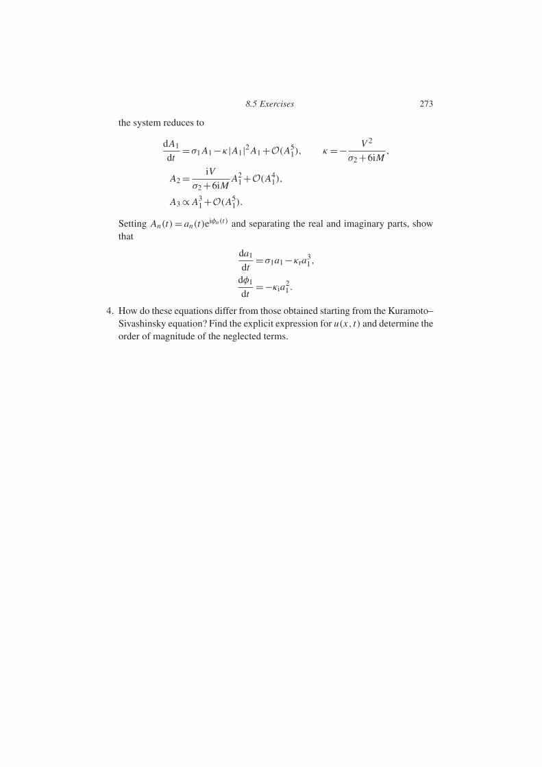
8.5 Exercises 273

the system reduces to

dA1

dt=σ1 A1 −κ|A1|2 A1 +O(A5

1), κ =− V 2

σ2 +6iM,

A2 = iV

σ2 +6iMA2

1 +O(A41),

A3 ∝ A31 +O(A5

1).

Setting An(t)= an(t)eiφn(t) and separating the real and imaginary parts, showthat

da1

dt=σ1a1 −κra

31,

dφ1

dt=−κia

21 .

4. How do these equations differ from those obtained starting from the Kuramoto–Sivashinsky equation? Find the explicit expression for u(x, t) and determine theorder of magnitude of the neglected terms.

9

Nonlinear dispersive waves

9.1 Introduction

When a fluid is locally perturbed by an impulse (for example, by an impact) ora periodic excitation (the vibration of a membrane, string, or mechanical blade),the perturbation may propagate from the source in the form of a wave. Exam-ples include acoustic waves, surface waves, and internal waves in a stratified fluid(Lighthill, 1978). The solution of the linearized equations for small amplitude per-turbations leads to a major result: the wave number k and frequency ω (or thewave speed c=ω/k) are not independent, they are related by a dispersion relation.Since this relation is obtained from linearized equations, another major result isthat dispersion does not depend on the amplitude of the perturbation. However,if the amplitude exceeds some level, new effects arise that the dispersion relationof linear theory obviously does not describe. To explain these new effects it isnecessary to include nonlinear terms neglected in the linear study, i.e., to developa theory of nonlinear waves. Such waves are also referred to as finite-amplitudewaves, in contrast to the waves of infinitesimal amplitude considered in a linearanalysis.

The objective of the present chapter is to give an elementary account of thetheory of nonlinear waves. We will show (i) how nonlinear waves can be con-structed by a perturbation method (essentially the multiple-scale method presentedin the preceding chapter), and (ii) how the linear stability of these waves can bestudied. This analysis is based on a great classic of hydrodynamics, the problemof gravity waves. Its analysis was initiated by G. G. Stokes (1847), who made adecisive advance in the field: a history of further developments in the field canbe found in the articles by A. D. D. Craik (2004, 2005) and O. Darrigol (2003,2005). Gravity waves have become a paradigm for nonlinear waves: the studyof waves in elastic solids, optical or electromagnetic waves, and, more gener-ally, waves propagating in weakly dissipative dispersive media is based on the

274

9.2 Instability of gravity waves 275

same ideas and uses the same analysis techniques (Whitham, 1974; Billinghamand King, 2000). In this chapter we shall neglect dissipative effects, which wejustify by considering the orders of magnitude: for a gravity wave of wavelength100 m in deep water, the ratio of the inertial forces to the viscous forces is of orderω/νk2 =√

gk/νk2 = 2×108. Dissipative effects will be reintroduced in the nextchapter.

In the following section we present the nonlinear Stokes wave along with theexperimental evidence for its instability (Benjamin and Feir, 1967). This instabilitycan be interpreted in two different ways (thus highlighting two different aspects ofthe problem), namely in terms of resonances among Fourier modes, or in terms ofthe modulation instability of the envelope of a quasi-monochromatic wave. Thesetwo interpretations are presented in Sections 9.3 and 9.4. The ideas and calcula-tional methods are illustrated by the model problem of masses coupled by springs,where the continuum limit is governed by a classical equation of field theory, theKlein–Gordon equation. This model problem has the advantage of containing allthe essential physics (dispersion and nonlinearities), while requiring much lesscomputing than typical hydrodynamics problems. In the final section of the chapterwe return to the problem of resonances.

9.2 Instability of gravity waves

9.2.1 Stokes waves

Let us consider a gravity wave propagating on the surface of a deep fluid, whereviscosity and surface tension effects are negligible. If we further assume the motionto be irrotational, the velocity field is governed by Laplace’s equation for the veloc-ity gradient. The condition of constant pressure at the interface then couples thevelocity potential to the pressure and the wave height through Bernoulli’s equation.For a wave of wave number k0, frequency ω0, small amplitude a0 (more precisely,wave slope k0a0 1), and large fluid depth h (more precisely, k0h 1), solu-tion of the linearized problem for small amplitude waves on deep water gives thedispersion relation (see Chapter 2, or Lighthill (1978)):

ω20 = gk0. (9.1)

However, observation shows that a gravity wave on the surface of the ocean,for example, differs from a sinusoidal wave: it displays sharper crests and flattertroughs. This implies that the wave profile contains harmonics and that these har-monics propagate at the same speed as the fundamental. However, this is forbiddenby the expression (9.1), which means that nonlinear phenomena must be involved.Furthermore, observation shows that the relation (9.1) is not really accurate. We

276 Nonlinear dispersive waves

0 2π 4π

−1

0

1

kx

η/a

Figure 9.1 (—) Stokes wave (9.2) for ka =0.4; (– · –) a sinusoidal wave.

are indebted to Stokes (1847) for resolving these issues. Using a series expansionin powers of the wave slope, the profile of the free surface η(x, t) is found to be(Lamb, 1932, §250; Whitham, 1974, §13.13)

η(x, t)

a0= k0a0

2+cosθ + k0a0

2cos2θ + 3(k0a0)

2

8cos3θ +O[(k0a0)

3], (9.2)

where the phase θ and the frequency ω are defined as

θ = k0x −ωt, ω2 =ω201+k2

0a20 +O[(k0a0)

4].

The profile of this wave is shown in Figure 9.1, where we compare it to a sinu-soidal wave. Its frequency ω is not quite equal to the frequency ω0 of a wave ofinfinitesimal amplitude; to leading order it is given by

ω

ω0=1+ 1

2k2

0a20 . (9.3)

These results display two qualitatively new phenomena compared to the lin-ear theory. The first is that a wave of finite amplitude can propagate withoutdeformation, with the harmonics propagating at the same speed as the funda-mental (which a priori is not at all obvious since linear waves are dispersive).The second is that the dispersion relation (9.3) involves the amplitude: the fre-quency of a wave of wave number k0, and therefore the wave speed c0 =ω0/k0,grows with the amplitude. Thus we have a wave of permanent form that exhibitsboth wave number dispersion and amplitude dispersion. In Exercise 9.6.2 we pro-pose the calculation of a nonlinear wave similar to (9.2) using the Klein–Gordonequation.

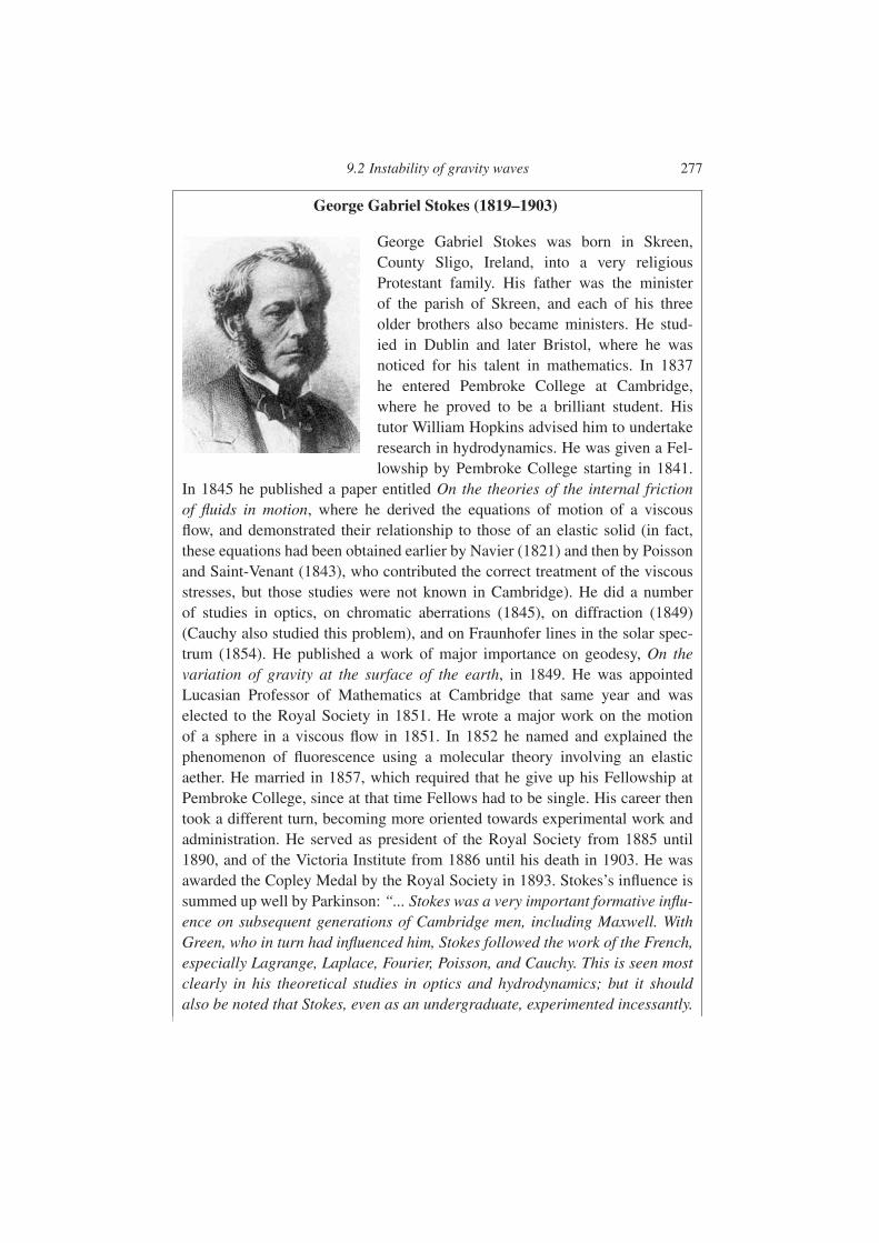
9.2 Instability of gravity waves 277

George Gabriel Stokes (1819–1903)

George Gabriel Stokes was born in Skreen,County Sligo, Ireland, into a very religiousProtestant family. His father was the ministerof the parish of Skreen, and each of his threeolder brothers also became ministers. He stud-ied in Dublin and later Bristol, where he wasnoticed for his talent in mathematics. In 1837he entered Pembroke College at Cambridge,where he proved to be a brilliant student. Histutor William Hopkins advised him to undertakeresearch in hydrodynamics. He was given a Fel-lowship by Pembroke College starting in 1841.

In 1845 he published a paper entitled On the theories of the internal frictionof fluids in motion, where he derived the equations of motion of a viscousflow, and demonstrated their relationship to those of an elastic solid (in fact,these equations had been obtained earlier by Navier (1821) and then by Poissonand Saint-Venant (1843), who contributed the correct treatment of the viscousstresses, but those studies were not known in Cambridge). He did a numberof studies in optics, on chromatic aberrations (1845), on diffraction (1849)(Cauchy also studied this problem), and on Fraunhofer lines in the solar spec-trum (1854). He published a work of major importance on geodesy, On thevariation of gravity at the surface of the earth, in 1849. He was appointedLucasian Professor of Mathematics at Cambridge that same year and waselected to the Royal Society in 1851. He wrote a major work on the motionof a sphere in a viscous flow in 1851. In 1852 he named and explained thephenomenon of fluorescence using a molecular theory involving an elasticaether. He married in 1857, which required that he give up his Fellowship atPembroke College, since at that time Fellows had to be single. His career thentook a different turn, becoming more oriented towards experimental work andadministration. He served as president of the Royal Society from 1885 until1890, and of the Victoria Institute from 1886 until his death in 1903. He wasawarded the Copley Medal by the Royal Society in 1893. Stokes’s influence issummed up well by Parkinson: “... Stokes was a very important formative influ-ence on subsequent generations of Cambridge men, including Maxwell. WithGreen, who in turn had influenced him, Stokes followed the work of the French,especially Lagrange, Laplace, Fourier, Poisson, and Cauchy. This is seen mostclearly in his theoretical studies in optics and hydrodynamics; but it shouldalso be noted that Stokes, even as an undergraduate, experimented incessantly.

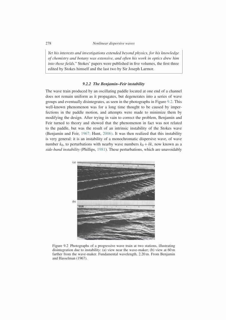
278 Nonlinear dispersive waves

Yet his interests and investigations extended beyond physics, for his knowledgeof chemistry and botany was extensive, and often his work in optics drew himinto those fields.” Stokes’ papers were published in five volumes, the first threeedited by Stokes himself and the last two by Sir Joseph Larmor.

9.2.2 The Benjamin–Feir instability

The wave train produced by an oscillating paddle located at one end of a channeldoes not remain uniform as it propagates, but degenerates into a series of wavegroups and eventually disintegrates, as seen in the photographs in Figure 9.2. Thiswell-known phenomenon was for a long time thought to be caused by imper-fections in the paddle motion, and attempts were made to minimize them bymodifying the design. After trying in vain to correct the problem, Benjamin andFeir turned to theory and showed that the phenomenon in fact was not relatedto the paddle, but was the result of an intrinsic instability of the Stokes wave(Benjamin and Feir, 1967; Hunt, 2006). It was then realized that this instabilityis very general: it is an instability of a monochromatic dispersive wave, of wavenumber k0, to perturbations with nearby wave numbers k0 + δk, now known as aside-band instability (Phillips, 1981). These perturbations, which are unavoidably

(a)

(b)

Figure 9.2 Photographs of a progressive wave train at two stations, illustratingdisintegration due to instability: (a) view near the wave-maker; (b) view at 60 mfarther from the wave-maker. Fundamental wavelength, 2.20 m. From Benjaminand Hasselman (1967).

9.3 Instability due to resonant interactions 279

present in any experiment, grow exponentially via a resonance mechanism when

δk2

k20

<8(k0a0)2, (9.4)

that is, when their wave number lies in a narrow band about k0. Using the disper-sion relation (9.1), the frequency of these perturbations is found to lie inside thenarrow range ω0(1±√

2k0a0). The two most highly amplified perturbations arethose with wave numbers k0(1±2k0a0), and their growth rate is

σmax = ω0

2(k0a0)

2. (9.5)

We note that this maximum growth rate is equal to the nonlinear correction to thefrequency, see (9.3).

The experiments performed by Lake et al. (1977) confirmed Benjamin’s anal-ysis, as shown in Figures 9.3, 9.4, and 9.5. Figure 9.3 shows time recordings ofthe interface position at various distances from the paddle; the amplification of themodulations is clearly seen. Figure 9.4 shows the corresponding amplitude spectra,which display the growth of wave numbers close to the fundamental. The growthof perturbations with frequency close to those of the harmonics is also clearly seen.Figure 9.5 compares the measurements by Lake et al. (1977) of the growth of theamplitude of the perturbation to the predictions of Benjamin and Feir (1967); theagreement is seen to be excellent.

As announced in the introduction, rather than presenting the hydrodynamicalstudy of Benjamin and Feir, here we shall discuss a simpler model problem illus-trating the general nature of the side-band instability of a dispersive nonlinearwave.

9.3 Instability due to resonant interactions

9.3.1 The model problem

The model equation used here to display the instability of a wave due to resonantinteractions is the nonlinear Klein–Gordon equation:

∂2u

∂t2− ∂2u

∂x2=−V ′(u), V (u)= u2

2+γ u4, (9.6)

where V ′(u) is the derivative of the potential V (u) and γ is a real parameter.This equation is a generalization of the classical equation for linear waves which

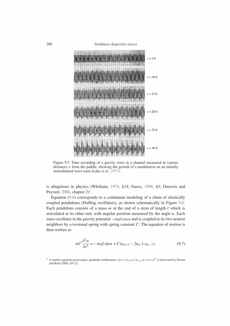
280 Nonlinear dispersive waves

x = 5 ft

x = 10 ft

x = 15 ft

x = 20 ft

x = 25 ft

x = 30 ft

Figure 9.3 Time recording of a gravity wave in a channel measured at variousdistances x from the paddle, showing the growth of a modulation on an initiallyunmodulated wave train (Lake et al., 1977).

is ubiquitous in physics (Whitham, 1974, §14; Fauve, 1998, §3; Dauxois andPeyrard, 2006, chapter 2)1.

Equation (9.6) corresponds to a continuum modeling of a chain of elasticallycoupled pendulums (Duffing oscillators), as shown schematically in Figure 9.6.Each pendulum consists of a mass m at the end of a stem of length l which isarticulated at its other end, with angular position measured by the angle u. Eachmass oscillates in the gravity potential −mgl cosu and is coupled to its two nearestneighbors by a torsional spring with spring constant C . The equation of motion isthen written as

ml2 ∂2u

∂t2=−mgl sinu +C(un+1 −2un +un−1). (9.7)

1 A similar equation possessing a quadratic nonlinearity, ∂t t u +∂xx u +∂xxxx u +u =u2, is discussed by Drazinand Reid (2004, §51.2).

9.3 Instability due to resonant interactions 281

(a) (b) (c) (d)

Frequency (Hz)

PSD

(V

2/H

z ∝

a2/H

z)

Figure 9.4 Power spectra (PSD = power spectral density) corresponding to thetime recordings in Figure 9.3: (a) x =5 ft, (b) x =10 ft, (c) x =20 ft, (d) x =30 ft(Lake et al., 1977).

In the limit where the wavelengths in question are large compared to the distancebetween two oscillators, (9.7) reduces to the equation ∂t t u − ∂xx u = −sinu (thesine-Gordon equation) after an appropriate choice of the time, mass, and lengthscales.2 For small amplitudes the sine-Gordon equation corresponds to the Klein–Gordon equation (9.6) with γ =−1/24.

9.3.2 A nonlinear Klein–Gordon wave

The dispersion relation

Linearizing (9.6) about the base solution u = 0 and using the normal modes u ∝ei(kx−ωt), we obtain the dispersion relation:

ω2 =1+k2. (9.8)

This relation shows that perturbations of infinitesimal amplitude propagate at aspeed c =ω/k depending on the wave number, so that waves are dispersive.

2 It is easy to recognize the nearest-neighbor interaction terms as being related to the centered finite differenceapproximation for ∂xx u.

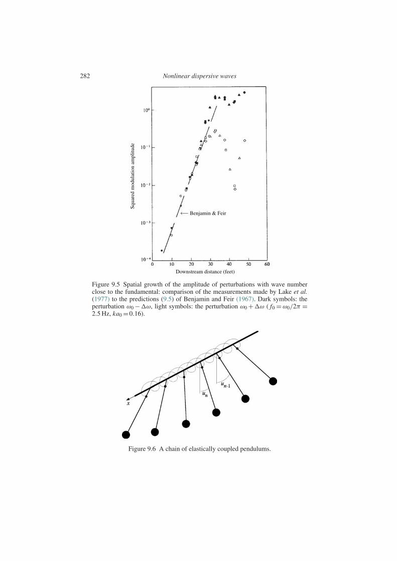
282 Nonlinear dispersive waves

Downstream distance (feet)

Benjamin & Feir

Squa

red

mod

ulat

ion

ampl

itude

Figure 9.5 Spatial growth of the amplitude of perturbations with wave numberclose to the fundamental: comparison of the measurements made by Lake et al.(1977) to the predictions (9.5) of Benjamin and Feir (1967). Dark symbols: theperturbation ω0 −ω, light symbols: the perturbation ω0 +ω ( f0 =ω0/2π =2.5 Hz, ka0 =0.16).

Figure 9.6 A chain of elastically coupled pendulums.

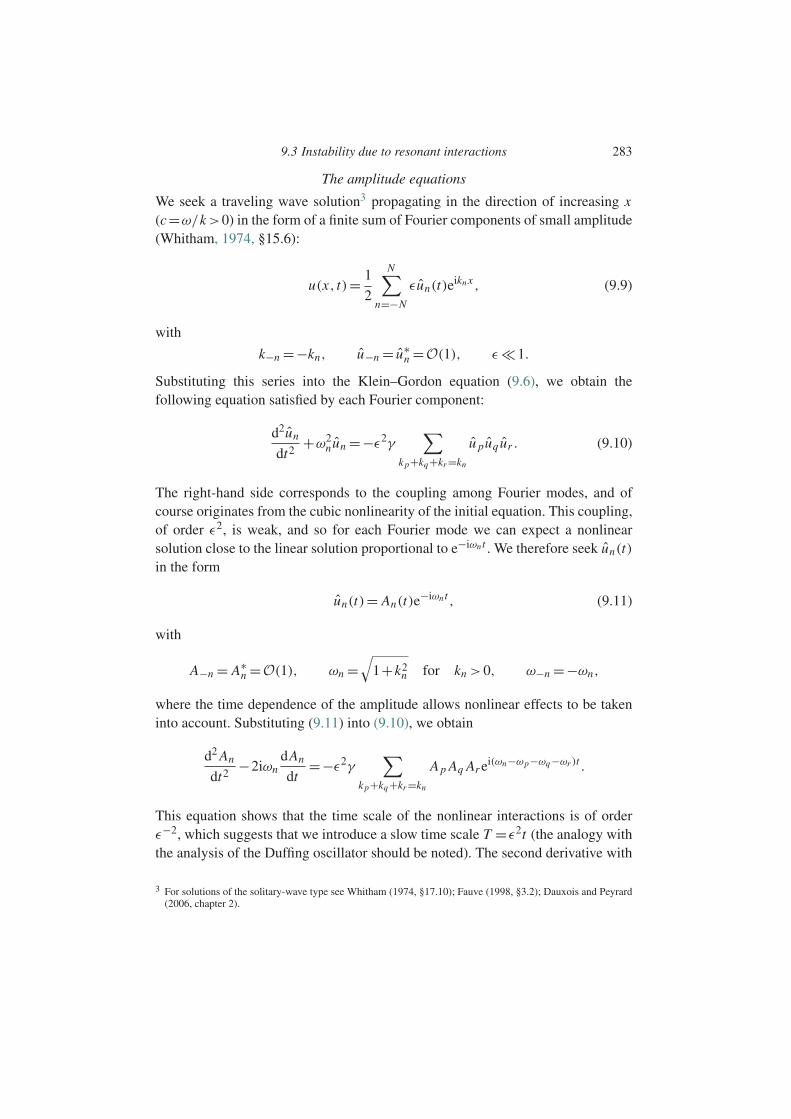
9.3 Instability due to resonant interactions 283

The amplitude equations

We seek a traveling wave solution3 propagating in the direction of increasing x(c=ω/k >0) in the form of a finite sum of Fourier components of small amplitude(Whitham, 1974, §15.6):

u(x, t)= 1

2

N∑n=−N

εun(t)eikn x , (9.9)

with

k−n =−kn, u−n = u∗n =O(1), ε 1.

Substituting this series into the Klein–Gordon equation (9.6), we obtain thefollowing equation satisfied by each Fourier component:

d2un

dt2+ω2

nun =−ε2γ∑

kp+kq+kr =kn

u puq ur . (9.10)

The right-hand side corresponds to the coupling among Fourier modes, and ofcourse originates from the cubic nonlinearity of the initial equation. This coupling,of order ε2, is weak, and so for each Fourier mode we can expect a nonlinearsolution close to the linear solution proportional to e−iωnt . We therefore seek un(t)in the form

un(t)= An(t)e−iωnt , (9.11)

with

A−n = A∗n =O(1), ωn =

√1+k2

n for kn >0, ω−n =−ωn,

where the time dependence of the amplitude allows nonlinear effects to be takeninto account. Substituting (9.11) into (9.10), we obtain

d2 An

dt2−2iωn

dAn

dt=−ε2γ

∑kp+kq+kr =kn

Ap Aq Ar ei(ωn−ωp−ωq−ωr )t .

This equation shows that the time scale of the nonlinear interactions is of orderε−2, which suggests that we introduce a slow time scale T =ε2t (the analogy withthe analysis of the Duffing oscillator should be noted). The second derivative with

3 For solutions of the solitary-wave type see Whitham (1974, §17.10); Fauve (1998, §3.2); Dauxois and Peyrard(2006, chapter 2).

284 Nonlinear dispersive waves

respect to time then appears as a negligible term of order ε4, and we obtain theamplitude equation for the nth mode:

dAn

dT=− iγ

2ωn

∑kp+kq+kr =kn

Ap Aq Ar ei(ωn−ωp−ωq−ωr )T/ε2. (9.12)

This equation corresponds to an interaction among Fourier modes whose wavenumbers satisfy the condition kp +kq +kr = kn . This interaction leads to remark-able solutions, in particular, when the argument of the exponential vanishes, thatis, when the frequencies satisfy the resonance condition

ωp +ωq +ωr =ωn. (9.13)

We note that owing to the dispersion relation (9.8), the quadruplets of waves whichsatisfy kp + kq + kr = kn , together with the above resonance equation, are veryspecial.

A monochromatic nonlinear wave

Let us consider the simple and important case of the resonant interaction of amonochromatic wave of wave number k0 with itself (self-interaction). The sum-mation in (9.9) runs over the two wave numbers k0 and −k0. Among the 23 triads(±k0,±k0,±k0), only three satisfy the condition kp + kq + kr = k0 and the reso-nance condition (9.13), namely, (k0,k0,−k0), (k0,−k0,k0), and (−k0,k0,k0). Theamplitude equation (9.12) for A0 then reduces to

dA0

dT=−iβA2

0 A∗0, (9.14)

with

β = 3γ

2ω0, ω0 =

√1+k2

0 .

The solution of this equation is

A0 =a0e−iβa20 T , a0 =O(1) real, (9.15)

or, returning to the original angular variable u(x, t),

u(x, t)= εa0 cos(k0x −ωt)+O(ε3), (9.16a)

ω=ω0 +β(εa0)2, (9.16b)

which is valid for t of order ε−2.Therefore, the frequency and speed of the wave of finite amplitude (9.16) are

modified by the self-interaction due to the cubic nonlinearity of the Klein–Gordon

9.3 Instability due to resonant interactions 285

equation, so that now they depend on the amplitude. We note that the frequencycorrection is exactly the same as that of a simple Duffing oscillator! Moreover, thiscorrection is very similar to the result (9.2)–(9.3) obtained by Stokes for gravitywaves. A more complete calculation including two harmonics is the subject of anexercise.

9.3.3 Instability of a monochromatic nonlinear wave

Instability of the Klein–Gordon wave (9.16)

Let us now consider the effect of a perturbation of the monochromatic wave (9.16)in the form of two waves with wave numbers k0 ± εK , K =O(1), close to k0,frequencies ω±, and amplitudes |A±| |A0|. Keeping only the dominant terms,the system (9.12) reduces to

dA0

dT=−iβA2

0 A∗0, β = 3γ

2ω0, ω0 =

√1+k2

0, (9.17a)

dA−dT

=−iβ(2A0 A∗0 A−+ A2

0 A∗+eiT ), (9.17b)

dA+dT

=−iβ(2A0 A∗0 A++ A2

0 A∗−eiT ), (9.17c)

with

= 1

ε2(ω++ω−−2ω0)≈ω′′

0 K 2 =O(1), ω′′0 = ∂2ω

∂k2(k0)=ω−3

0 .

Equation (9.17a), which is identical to (9.14), describes the self-interaction, and itssolution is given by (9.15) (the effect of the perturbations on A0 is of higher order).Equations (9.17b) and (9.17c) describe the evolution of the perturbation: the firstterm on the right-hand sides corresponds to the exact resonance ω±=ω0−ω0+ω±and the second to a near-resonance. Substituting the solution (9.15) into (9.17b)and (9.17c), we find

dA−dT

=−iβa20

(2A−+ A∗

+ei(−2βa20)T), (9.18a)

dA+dT

=−iβa20

(2A++ A∗

−ei(−2βa20)T). (9.18b)

Replacing (9.18b) by its complex conjugate, we obtain a linear system in A− andA∗+ which is nonautonomous (it depends explicitly on time). This system can bemade autonomous by the change of variable B± = A±eiρT corresponding to arotation in the complex plane, and by substitution we easily find that we requireρ=βa2

0 −/2. The resulting system is an eigenvalue problem which has solutions

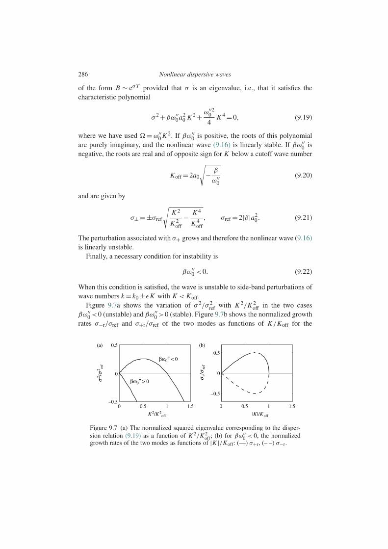
286 Nonlinear dispersive waves

of the form B ∼ eσT provided that σ is an eigenvalue, i.e., that it satisfies thecharacteristic polynomial

σ 2 +βω′′0a2

0 K 2 + ω′′20

4K 4 =0, (9.19)

where we have used =ω′′0 K 2. If βω′′

0 is positive, the roots of this polynomialare purely imaginary, and the nonlinear wave (9.16) is linearly stable. If βω′′

0 isnegative, the roots are real and of opposite sign for K below a cutoff wave number

Koff =2a0

√− β

ω′′0

(9.20)

and are given by

σ± =±σref

√K 2

K 2off

− K 4

K 4off

, σref =2|β|a20 . (9.21)

The perturbation associated with σ+ grows and therefore the nonlinear wave (9.16)is linearly unstable.

Finally, a necessary condition for instability is

βω′′0 <0. (9.22)

When this condition is satisfied, the wave is unstable to side-band perturbations ofwave numbers k = k0 ±εK with K < Koff.

Figure 9.7a shows the variation of σ 2/σ 2ref with K 2/K 2

off in the two casesβω′′

0 <0 (unstable) and βω′′0 >0 (stable). Figure 9.7b shows the normalized growth

rates σ−r/σref and σ+r/σref of the two modes as functions of K/Koff for the

0.5(a) (b)

0.5

0

–0.5

0

–0.50 0.5 1.5

βω0″ < 0

βω0″ > 0

K2/K2off

|K |/Koff

σ2 /σ

2 ref

σr/

σre

f

1 0 0.5 1.51

Figure 9.7 (a) The normalized squared eigenvalue corresponding to the disper-sion relation (9.19) as a function of K 2/K 2

off; (b) for βω′′0 < 0, the normalized

growth rates of the two modes as functions of |K |/Koff: (—) σ+r, (– –) σ−r.

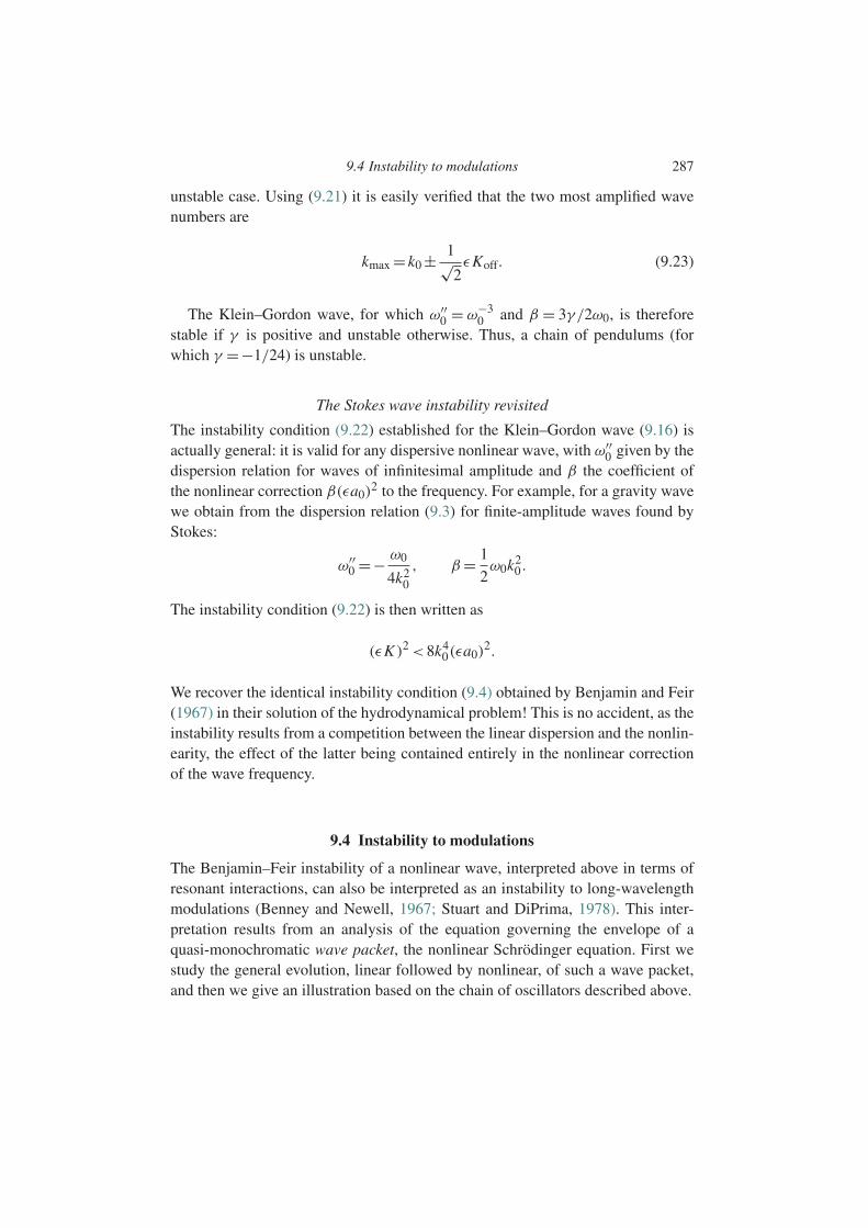
9.4 Instability to modulations 287

unstable case. Using (9.21) it is easily verified that the two most amplified wavenumbers are

kmax = k0 ± 1√2εKoff. (9.23)

The Klein–Gordon wave, for which ω′′0 = ω−3

0 and β = 3γ /2ω0, is thereforestable if γ is positive and unstable otherwise. Thus, a chain of pendulums (forwhich γ =−1/24) is unstable.

The Stokes wave instability revisited

The instability condition (9.22) established for the Klein–Gordon wave (9.16) isactually general: it is valid for any dispersive nonlinear wave, with ω′′

0 given by thedispersion relation for waves of infinitesimal amplitude and β the coefficient ofthe nonlinear correction β(εa0)

2 to the frequency. For example, for a gravity wavewe obtain from the dispersion relation (9.3) for finite-amplitude waves found byStokes:

ω′′0 =− ω0

4k20

, β = 1

2ω0k2

0 .

The instability condition (9.22) is then written as

(εK )2 <8k40(εa0)

2.

We recover the identical instability condition (9.4) obtained by Benjamin and Feir(1967) in their solution of the hydrodynamical problem! This is no accident, as theinstability results from a competition between the linear dispersion and the nonlin-earity, the effect of the latter being contained entirely in the nonlinear correctionof the wave frequency.

9.4 Instability to modulations

The Benjamin–Feir instability of a nonlinear wave, interpreted above in terms ofresonant interactions, can also be interpreted as an instability to long-wavelengthmodulations (Benney and Newell, 1967; Stuart and DiPrima, 1978). This inter-pretation results from an analysis of the equation governing the envelope of aquasi-monochromatic wave packet, the nonlinear Schrodinger equation. First westudy the general evolution, linear followed by nonlinear, of such a wave packet,and then we give an illustration based on the chain of oscillators described above.

288 Nonlinear dispersive waves

9.4.1 Linear dynamics of a wave packet: envelope equation

Let us resume our study of the propagation and dispersion of a wave packet begunin Chapter 3 with the ultimate goal of including nonlinear effects. We consider awave represented by the Fourier integral

u(x, t)= 1

2

∫ +∞

−∞u(k)ei(kx−ωt)dk, (9.24)

where ω=ω(k) is a real branch of the dispersion relation corresponding to prop-agation in the direction of increasing x , so that ω(−k)=−ω(k) (for example, fora gravity wave in deep water ω = +√

gk for k > 0 and ω = −√−gk for k < 0).Since u(x, t) is real, we must have u∗(k)= u(−k), and the above integral can alsobe written as

u(x, t)= 1

2

∫ +∞

0u(k)ei(kx−ω(k)t)dk +c.c. (9.25)

Let us now assume that u(x, t) is a wave packet of width δk centered on the wavenumber k0, i.e., that the complex amplitudes u(k) are nonzero only in a narrowband centered on k0 (Lighthill, 1978, §3.7; Whitham, 1974, §17.7). Isolating thedominant monochromatic wave, the packet can be written as

u(x, t)= 1

2A(x, t)ei(k0x−ω0t)+c.c., (9.26)

where ω0 =ω(k0) and the envelope A(x, t) of the wave packet is defined as

A(x, t)=∫ +∞

0u(k)ei(k−k0)x−i(ω(k)−ω0)t dk. (9.27)

Since the amplitudes u(k) are zero outside a distance δk from k0, the integrationcan be restricted to this range, with the frequency ω(k) given by a Taylor seriesexpansion about k0. Truncating it at second order, we have

ω−ω0 = cg(k −k0)+ω′′

0

2(k −k0)

2 ,

where the group velocity cg and the coefficient ω′′0 are given by

cg = ∂ω

∂k(k0), ω′′

0 = ∂2ω

∂k2(k0).

Substituting this series into (9.27), we recognize it as the general solution (acontinuous sum of Fourier modes) of the envelope equation

i∂t A =−icg ∂x A+α∂xx A, α= 1

2ω′′

0 . (9.28)

9.4 Instability to modulations 289

This linear equation therefore gives a generic description of the linear evolutionof the envelope A(x, t) of a dispersive wave packet centered on k0. This packetpropagates at the group velocity cg and, since the dispersion causes different wavenumbers to propagate at slightly different speeds, the width of the packet growslinearly in time while its amplitude decreases as 1/

√t .

9.4.2 Nonlinear dynamics: the nonlinear Schrodinger equation

What sort of influences do nonlinear effects have on the dispersion of a wavepacket? To answer this question we can seek the dominant nonlinear term to beadded to the envelope equation (9.28). The form of this term can be deduced fromsymmetry arguments (Fauve, 1998). Let us assume that the problem is invariantunder translations x → x + ξ and t → t + τ , as in the coupled pendulum prob-lem studied earlier. Then if A is the solution of the amplitude equation, Aeiφ

corresponding to a wave with phase shifted by φ must also be a solution. Theequation must therefore be invariant under the transformation A → Aeiφ , and theterm of lowest degree possessing this property, which dominates for small u(x, t),is |A|2 A. In a reference frame undergoing translation at the group velocity cg, theenvelope equation is therefore the nonlinear Schrodinger equation:

i∂t A =α∂xx A−β |A|2 A. (9.29)

Moreover, if the problem is invariant under reflections x →−x and t →−t (againlike the coupled pendulum problem), the coefficient β must be real. Then in viewof these symmetries, if u(x, t) is a solution, u(−x,−t) must also be one (the tworeflections being applied simultaneously in order to preserve the propagation direc-tion of the wave). Therefore, if A(x, t) is a solution of (9.29), A∗(−x,−t) mustalso be a solution owing to (9.26). The Schrodinger equation (9.29) must thereforebe invariant under the transformations x →−x , t →−t , and A → A∗, and so it iswritten as

−i∂t A∗ =α∂xx A∗−β |A|2 A∗.

Taking the complex conjugate of this equation, we obtain (9.29) with β∗ instead ofβ. We therefore have β∗=β, from which we see that β is real. However, symmetryarguments do not allow us to determine the coefficient β, and in particular its sign,on which the wave stability depends. This coefficient is determined below in thesimple case of the nonlinear Klein–Gordon equation.

We note that the Schrodinger equation possesses the same cubic nonlinearity asthe Landau equation, and that in place of the amplification term σ A it involves adiffusion term α∂xx A (up to a factor of i).

290 Nonlinear dispersive waves

The nonlinear Schrodinger equation (9.29) (often abbreviated as NLS) arises inmany areas of physics (electric circuits, fiber optics, plasmas) and biology (DNAdynamics) (Dauxois and Peyrard, 2006, chapter 3). In hydrodynamics this equationwas first obtained by Benney and Newell (1967) in describing the weakly nonlin-ear dynamics of slow modulations of gravity waves in deep water. These authorsactually studied a slightly more general problem including modulations in thetransverse spatial direction y.

9.4.3 Stability of a quasi-monochromatic wave

The nonlinear Schrodinger equation (9.29) admits the spatially uniform solution

A0 =a0ei(t+), a0 =|A0| real, =βa20, (9.30)

which corresponds to the unmodulated traveling wave

u(x, t)=a0 cos(k0x −ωt +), ω=ω0 +βa20, (9.31)

where is an undetermined phase associated with the translational invariance ofthe original problem. This solution shows that the nonlinear Schrodinger equationdescribes a remarkable phenomenon: a cubic nonlinearity can counteract the lin-ear dispersion so as to support a wave which propagates without deformation. Thisresult, which Stokes obtained in the special case of gravity waves, is therefore verygeneral, and is valid for all dispersive waves of finite amplitude described gener-ically (for the same symmetries) by the Schrodinger equation. We note that thisequation also admits localized solutions which we shall not discuss here (Fauve,1998; Dauxois and Peyrard, 2006, chapter 3).

We can study the stability of this wave by perturbing the solution A0 as

A(x, t)= (a0 +a(x, t))ei(t++ϕ(x,t)) (9.32)

and substituting this expression into Eq. (9.29). After linearizing and separatingthe real and imaginary parts, we obtain

∂a

∂t=αa0

∂2ϕ

∂x2, (9.33a)

∂ϕ

∂t=2βa0a − α

a0

∂2a

∂x2. (9.33b)

This linear system with constant coefficients admits solutions of the form eσ t−ipx

if its determinant vanishes, that is, if p and σ satisfy the dispersion relation

σ 2 +2αβa20 p2 +α2 p4 =0. (9.34)

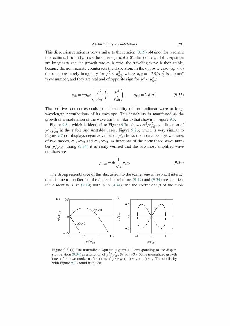
9.4 Instability to modulations 291

This dispersion relation is very similar to the relation (9.19) obtained for resonantinteractions. If α and β have the same sign (αβ >0), the roots σ± of this equationare imaginary and the growth rate σr is zero; the traveling wave is then stable,because the nonlinearity counteracts the dispersion. In the opposite case (αβ < 0)the roots are purely imaginary for p2 > p2

off, where poff = −2β/αa20 is a cutoff

wave number, and they are real and of opposite sign for p2 < p2off:

σ± =±σref

√√√√ p2

p2off

(1− p2

p2off

), σref =2|β|a2

0 . (9.35)

The positive root corresponds to an instability of the nonlinear wave to long-wavelength perturbations of its envelope. This instability is manifested as thegrowth of a modulation of the wave train, similar to that shown in Figure 9.3.

Figure 9.8a, which is identical to Figure 9.7a, shows σ 2/σ 2ref as a function of

p2/p2off in the stable and unstable cases. Figure 9.8b, which is very similar to

Figure 9.7b (it displays negative values of p), shows the normalized growth ratesof two modes, σ−r/σref and σ+r/σref, as functions of the normalized wave num-ber p/poff. Using (9.34) it is easily verified that the two most amplified wavenumbers are

pmax =± 1√2

poff. (9.36)

The strong resemblance of this discussion to the earlier one of resonant interac-tions is due to the fact that the dispersion relations (9.19) and (9.34) are identicalif we identify K in (9.19) with p in (9.34), and the coefficient β of the cubic

0.5(a) (b)

0.5

0

–0.5

0

–0.50 0.5 1.5 –1 0 1

αβ < 0

αβ > 0

p2/p2off p/poff

σ2 /σ

2 ref

σr/

σre

f

1

Figure 9.8 (a) The normalized squared eigenvalue corresponding to the disper-sion relation (9.34) as a function of p2/p2

off; (b) for αβ<0, the normalized growthrates of the two modes as functions of p/poff: (—) σ+r, (– –) σ−r. The similaritywith Figure 9.7 should be noted.

292 Nonlinear dispersive waves

nonlinearity in (9.14) with that in the Schrodinger equation (9.29) (while not-ing that α = ω′′

0/2). This identification will become more clear in the followingsection, where we derive the Schrodinger equation for the Klein–Gordon wave.The situation can finally be summarized as follows:

• the dynamics of a dispersive wave of finite amplitude is generically governed bythe nonlinear Schrodinger equation;

• when the dispersion and the nonlinearity cooperate (αβ < 0) the wave is unsta-ble to long-wavelength modulations; conversely, when the steepening due tononlinearity is balanced by dispersion (αβ >0), the wave is stable;

• this instability is identical to the side-band instability due to resonant interactionwith nearby wave numbers discovered by Benjamin and Feir.

9.4.4 Interpretation in terms of phase instability

Let us very briefly show how the Benjamin–Feir instability can be interpretedin terms of phase dynamics. Differentiating the equation for the phase perturba-tion (9.33b) with respect to time and substituting the equation for the amplitudeperturbation (9.33a), we obtain the phase equation

∂t tϕ−2αβa20 ∂xxϕ+α2 ∂xxxxϕ=0.

This equation is a classical wave equation plus a fourth-order term which admitstraveling wave solutions of the form ϕ = ϕ(x ± ct) provided that c2 = 2αβa2

0 ispositive. It therefore appears that the instability condition αβ < 0 corresponds toan imaginary propagation velocity of the phase perturbations. We refer the readerto Manneville (1990) for a more general presentation of phase instabilities.

9.4.5 Derivation of the NLS equation for the Klein–Gordon wave

For the chain of oscillators shown in Figure 9.6 modeled by the Klein–Gordonequation (9.6), the coefficients of the linear terms in the Schrodinger equation areknown from the dispersion relation (9.8):

cg(k0)=ω′0 = k0

ω0, α= ω′′

0

2= 1

2ω30

.

Here the goal is to determine the dominant nonlinear term in the envelope equation,which can be done using the multiple-scale method. Let ε = δk/k0 1 be the rel-ative width of the wave packet. In a reference frame moving at the group velocitycg, two Fourier modes with wave numbers differing by δk have speeds whose

9.4 Instability to modulations 293

relative difference δc/c is of order δk/k0. This dispersion gives rise to a differ-ence on the order of a wavelength in the distance traveled over a time of order(k0δc)−1 = (εω0)

−1, after a distance traveled of order c/k0δc = (εk0)−1. These

dispersive effects are therefore manifested at long times of order T1 = εt =O(1)and over large distances of order X = εx =O(1). On the other hand, nonlineareffects are manifested only at even longer times of order T2 =ε2t . We therefore set

u(x, t)=u(x, t, X,T1,T2) (9.37)

and seek u as a series in powers of ε:

u = εu1 +ε2u2 + ... (9.38)

The calculations present no particular difficulty, so we omit the details. At orderε we find the following solution propagating in the positive x direction:

u1 = 1

2A(X,T1,T2)e

i(k0x−ω0t)+c.c., (9.39)

where ω0 =ω(k0) is given by the dispersion relation. At order ε2 the solvabilitycondition is written as

∂ A

∂T1=−cg

∂ A

∂X, cg = cg(k0)= k0

ω0, (9.40)

the solution of which is

A(X,T1,T2)= A(X −cgT1,T2). (9.41)

The interpretation of this result is that at the order we are studying the waveenvelope propagates at the group velocity without deformation.

At order ε3 the solvability condition gives the nonlinear Schrodinger equation:

i∂ A

∂T2=α

∂2 A

∂X2−β|A|2 A, α= ω′′

0

2= 1

2ω30

, β = 3γ

2ω0. (9.42)

This equation is identical to the nonlinear Schrodinger equation (9.29) up to thedefinition of the length and time scales, and the coefficient β is the same as in(9.14). This equation has the solution (9.30) corresponding to the nonlinear wave(9.16). In view of the stability results obtained in Section 9.4.3, we can concludethat the nonlinear wave solution of the Klein–Gordon equation (9.6) is unstablefor αβ negative, as for the chain of pendulums. These conclusions are of courseidentical to those obtained from the analysis in terms of resonant interactions.

294 Nonlinear dispersive waves

9.5 Resonances revisited

The Benjamin–Feir instability of a gravity wave to nearby wave numbers – orside-band instability – is a special case of instabilities resulting from a resonantinteraction among certain wave numbers. We conclude this chapter by discussinga resonance related to a quadratic nonlinearity.4

Let us consider a quadratically nonlinear problem with a solution u(x, t) givenby the Fourier sum

u(x, t)=∞∑

j=−∞A j e

i(k j x−ω(k j )t), A j = A(k j ). (9.43)

In the equation for the amplitude An (which we need not write) the quadraticnonlinearity leads to the appearance of a sum∑

kp+kq=kn

Ap Aqei(ωn−ωp−ωq )t (9.44)

analogous to that in Eq. (9.12). If the triad of numbers satisfying kp + kq = kn issuch that the frequencies obey the condition

ωn =ωp +ωq , (9.45)

it is said that the triad is resonant. Such a resonance does not necessarily imply theappearance of an instability, but greatly favors it.

The resonance condition (9.45) can be satisfied for gravity–capillary waves. Forsuch waves, the dispersion relation is given by

ω2 = gk + γ k3

ρ,

where ρ is the fluid density and γ is the surface tension. It can be verified thattriads such that k3 = k1 +k2 are resonant if the ratio r = k2/k1 obeys the relation(McGoldrick, 1965; Craik, 1985, chapter 5)

= (1+r2)+(1+r)(1+7r +r2)1/2

r(9+14r +9r2),

where = γ k21/2ρg. This equation can be arranged as a cubic polynomial in r

with coefficients depending on . A simple solution for =1/4 (corresponding toa wavelength λ1 =2.4 cm in water) is r =1, which corresponds to the triad

k1 = k2 =−k3/2.

4 A simple illustration of resonances with quadratic nonlinearity is treated in detail by Drazin and Reid (2004,§51), for a double pendulum.

9.6 Exercises 295

Therefore, a gravity–capillary wave can be unstable owing to interaction withitself and with a wave of half its wave number. This resonance is termed sub-harmonic. As another example, such triad resonances can also arise in stratifiedfluids between two surface waves and an internal wave. Note that if the waves canpropagate in more than one spatial direction, the condition on the wave numberskp +kq = kn becomes a condition on the wave vectors:

kn +kp +kq =0,

and the resonance condition is then less restrictive. Higher dimensionality istherefore more favorable to the appearance of resonances.

For gravity waves the dispersion relation forbids any triad resonances. There-fore, for waves of small slope ε = ka, no resonant interaction can appear at orderε2. Resonant interactions arise first at the following order ε3, among quadruplets.In particular, the interaction of the wave numbers

k, k, −k(1+ε), −k(1−ε),

with the respective frequencies

ω, ω, −ω(1+ 1

2ε), −ω(1− 1

2ε),

corresponds to the Benjamin–Feir instability. A deeper understanding of this sub-ject, due most notably to the work by Phillips and Benney in the early 1960s, canbe gained from the reviews by Phillips (1981), Hammack and Henderson (1993),and Dias and Kharif (1999).

9.6 Exercises

9.6.1 A nonlinear wave including two harmonics (1)

Consider a wave u(x, t) governed by the Klein–Gordon equation (9.6), of smallamplitude of order ε, composed of a fundamental harmonic k1 of amplitude εA1

and the second harmonic k2 =2k1 of amplitude εA2.

1. The summation in (9.9) runs over the four wave numbers ±k1 and ±k2. Showthat out of the 43 possible cubic products of wave numbers, there are only ninetriads (kp,kq ,kr ) satisfying k1 = kp +kq +kr . Show that they are all resonant,and that the same is true for triads satisfying k2 =kp +kq +kr . Derive the system

296 Nonlinear dispersive waves

of amplitude equations

dA1

dT=−iβA2

1 A∗1 −2iβA2 A∗

2 A1, (9.46a)

dA2

dT=−iβA2

2 A∗2 −2iβA1 A∗

1 A2, (9.46b)

with

β = 3γ

2ω10, ω10 =

√1+k2

1 .

2. Verify that this system has no nonzero solution that is independent of time.3. Find a solution for |A2| ∼ ε|A1| and derive the expression for u(x, t) (Craik,

1985, p. 177):

u(x, t)= εa1 cosθ +ε2a2 cos(2θ −k2(c1 −c2)t)+O(ε3),

with

θ = k1x −ω1t, ω1 =ω10 +βε2a21, c j =ω j/k j , a j =O(1), j =1,2.

Is the nonlinear frequency correction affected by the second harmonic? Whatcondition must the dispersion relation satisfy for the wave to propagate withoutdeformation? Can this condition be satisfied here?

4. A solution of the system of differential equations (9.46) can be found foramplitudes of the same order of magnitude, |A2| ∼ |A1| ∼ ε, by separating themodulus and the phase; the conclusions remain unchanged. It is also possi-ble to rework this exercise using the wave numbers k1 and k3 = 3k1. Are theconclusions unchanged in this case?

9.6.2 A nonlinear wave including two harmonics (2)

As shown by the preceding exercise, assuming that the amplitudes vary slowly canlead only to a small correction of order ε2 to the frequency and speed of the Fouriermodes. It is therefore impossible to construct a Stokes wave including harmonicswhich propagates without deformation, except in the special case of a subharmonicresonance where the harmonics have the same speed.5 The present exercise showshow to construct a nonlinear wave by “locking in” the speeds of the harmonics atthe start.

5 Such a resonance occurs, for example, in Kelvin–Helmholtz gravity–capillary waves for the triad (k,k,k/2);see Exercise 4.5.1, as well as Nayfeh and Saric (1972) and Craik (1985, §§14,19).

9.6 Exercises 297

1. We seek a nonlinear solution of the Klein–Gordon equation (9.6) in the “naive”form

u = εu1(θ)+ε3u3(3θ)+ ... , θ = kx −ω(k)t,

where ω(k) is a branch of solutions of the dispersion relation. Show that thesystem of equations obtained is

Lu1 =0, (9.47a)

Lu3 =−4γ u31, (9.47b)

where the operator L is defined by L = (ω2 −k2)∂θθ +1. Show that the solutionat order ε3 leads to the appearance of a secular (unbounded) term proportionalto θeiθ . (This is the same problem as that encountered in the naive solution ofthe Duffing oscillator; see Chapter 8.)

2. The difficulty encountered above, namely, the appearance of a secular term, isdue to the fact that we are seeking a nonlinear wave with frequency given by alinear dispersion relation. To resolve the difficulty we relax the wave frequencyby setting ω = ω0 + ε2ω2 + ..., which introduces an unknown correction ω2.Show that the system of equations to be solved is now

Lu1 =0, (9.48a)

Lu3 =−4γ u31 −2ω0ω2

∂2u1

∂θ2. (9.48b)

3. Show that the solution at order ε is

u1 = 1

2A1eiθ +c.c., θ = kx −ω0t,

and that the solvability condition at order ε3 implies that

ω2 = 3γ

2ω0a2, a =|A1|.

Show that the solution is given by

u(x, t)= εa cosθ + γ

8(εa)3 cos3θ +O(ε5), ω=ω0 + 3γ

2ω0(εa)2.

We note that the frequency correction obtained is identical to the correction(9.16b) found for a monochromatic wave by solving the amplitude equations(9.12), and also to the correction (9.42) found by calculating the cubic term inthe Schrodinger equation for the envelope of a wave packet.

298 Nonlinear dispersive waves

9.6.3 A nonlinear Korteweg–de Vries wave

Consider the Korteweg–de Vries equation (Boussinesq, 1871; Korteweg and deVries, 1895; Miles, 1981), which governs the dynamics of gravity waves ofwavelength long compared to the depth h (kh 1) (Whitham, 1974, §13.12–13):

∂tη+c0

(1+ 3

2

η

h

)∂xη+γ ∂xxxη=0, (9.49)

with

c0 =√

gh, γ = 1

6c0h2

(the Stokes calculation (1847) corresponds to the opposite limit kh 1). Fora wave of amplitude a and wave number k, the nonlinear term is of orderc0/hη∂xη ∼ c0kh(a/h)2 and the dispersion is of order c0h2∂xxxη ∼ c0h3k3a/h.When the two effects are of the same order of magnitude, that is, a/h ∼ k2h2, theabove equation admits localized solutions of the solitary wave type. The waves offinite amplitude we are seeking here can be obtained by an expansion in powers ofε =a/h with a/h k2h2.

Following the same method as in the preceding exercise, we therefore seek asolution of the form

η

h= εη1(θ)+ε2η2(2θ)+ ...

with

θ = kx −ωt, ω=ω0 +εω1 +ε2ω2 + ..., ω0 = c0k −γ k3.

(The first nonlinear correction is of order ε2 because the nonlinearity in theequation is quadratic.)

1. Show that there is no resonance at order ε2, so that we can set ω1 =0, and showthat the nonresonance (or solvability) condition at order ε3 is written as

ω2 = 3c20

32γ k.

2. Obtain the solution

η

h= ε cosθ + 3ε2

4k2h2cos2θ + 27ε3

64k4h4cos3θ + ... (9.50)

with

ω=ω0 + 9ε2

16k2h2.

10

Nonlinear dynamics of dissipative systems

10.1 Introduction

As we have discussed in earlier chapters, a dissipative physical system in a uni-form, stationary state can become linearly unstable when a control parameter Rexceeds a critical value Rc. This occurs, for example, in the instability of a fluidlayer heated from below governed by the Rayleigh number, or in the instabil-ity of plane Poiseuille flow governed by the Reynolds number. The instabilitycan be manifested as the appearance of a stationary, spatially periodic structure(Rayleigh–Benard convection rolls, for example), or as a growing traveling wave(Tollmien–Schlichting waves). This type of situation was studied in Chapter 8 forspatially confined systems, or systems with imposed periodicity, where the dynam-ics can be reduced to a system of differential equations for the amplitudes of a fewspatial harmonics. When the physical system is spatially extended, that is, when itssize is large compared to the wavelength of the periodic structure, the wave numberspectrum tends to become continuous, and spatial modulations of the amplitudescan arise. The appropriate formalism for describing these modulations is that ofenvelope equations.

In the present chapter we shall present this formalism and study the condi-tions for saturation of the primary instability arising at R = Rc, as well as forsecondary instabilities which arise when the bifurcation parameter exceeds a sec-ond threshold. First we study the case where the periodic structure is stationary,that is, where the eigenvalue of the linearized system crossing the imaginaryaxis at threshold R = Rc is real, i.e., the bifurcation is of the saddle–node orpitchfork type for a system possessing the reflection symmetry x −→ −x . Thecorresponding envelope equation is the Ginzburg–Landau equation with real coef-ficients. The secondary instability that typically arises in this situation is theEckhaus instability, as encountered prototypically in Rayleigh–Benard convectionand Couette–Taylor flow between two coaxial cylinders. We then present the case

299

300 Nonlinear dynamics of dissipative systems

of waves corresponding to a Hopf bifurcation (complex-conjugate eigenvalues).The corresponding envelope equation is the Ginzburg–Landau equation with com-plex coefficients. Here we recover the Benjamin–Feir instability introduced in theprevious chapter, and briefly discuss Tollmien–Schlichting waves again. The finalsection is devoted to the case where, owing to a particular symmetry, the wavenumber k =0 is neutral; accordingly, the dynamics of the mode of finite wave num-ber kc, which is marginal at threshold R = Rc, is strongly influenced by couplingto nearly neutral long-wavelength perturbations.

10.2 Weakly nonlinear dynamics

10.2.1 Linear evolution of a wave packet

Let us consider the case where, for a critical value Rc of a bifurcation parameterR, an instability of finite wave number kc and zero speed and group velocity (ω=∂ω/∂k = 0 at k = kc) appears, corresponding to an absolute instability. For r =R/Rc near rc =1, that is, for

ε2 = r −rc 1, (10.1)

the growth rate σ(k,r) near kc has the shape shown in Figure 10.1a: for r <rc, it isnegative for all wave numbers, and for r < rc there exists a band of unstable wavenumbers centered on rc, of width of order ε with growth rate of order ε2.

Let us expand this growth rate in a Taylor series near the critical point (kc,rc):

σ(k,r)=σ(kc,rc)+ ∂σ

∂k(k −kc)+ ∂σ

∂r(r −rc)+ 1

2

∂2σ

∂k2(k −kc)

2 + ·· · , (10.2)

where the derivatives are evaluated at the critical point (kc,rc). We shall see belowthat the omitted quadratic terms, proportional to (r −rc)

2 and (k −kc)(r −rc), aresmaller in order of magnitude than the term (k − kc)

2 that we have kept. In fact,two terms in the above Taylor expansion are zero: the growth rate σ(kc,rc), andthe term ∂σ/∂k since the curve σ(k) is tangent to the k-axis for r = rc. The aboveequation then reduces to

τc σ(k,r)= (r −rc)−ξ2c (k −kc)

2 + ·· · , (10.3)

where τc and ξc are characteristic time and length scales defined as

1

τc= ∂σ

∂r,

ξ2c

τc=−1

2

∂2σ

∂k2.

In the (k,r) plane the marginal stability curve, defined as σ(k,r)=0, is then givenby the parabola

r −rc = ξ2c (k −kc)

2

10.2 Weakly nonlinear dynamics 301

(a)

O(ε)

O(ε)

kc

kc k

rc

r

r > rc

r < rc

O(ε 2)

O(ε 2)

σ(b)

Unstable

Stable

Figure 10.1 (a) The growth rate σ(k) below and above threshold r = rc; (b) themarginal stability parabola σ =0.

and shown in Figure 10.1b. For r >rc and for a given ε2 =r −rc, the wave numbersinside the parabola are unstable and form a band whose width is of order εkc. Theterms omitted in (10.3) can therefore be seen to be at least of order ε3.

Now let us consider a perturbation of the base state, represented as in thepreceding chapter by a Fourier integral

u(x, t)= 1

2

∫ +∞

0u(k)eikx+σ(k)t dk +c.c. (10.4)

The perturbation can then be written as

u(x, t)= 1

2A(x, t)eikcx +c.c., (10.5)

where the envelope A(x, t) of the wave packet is defined as

A(x, t)=∫ +∞

0u(k)ei(k−kc)x+σ(k)t dk. (10.6)

This integral is dominated by wave numbers near kc (the other modes are stronglydamped), wherein σ(k) can be replaced by the Taylor series (10.3). We thenrecognize (10.6) as the general solution of the envelope equation

τc ∂tA= (r −rc)A+ξ2c ∂xxA. (10.7)

302 Nonlinear dynamics of dissipative systems

This equation describes the linear evolution of the envelope of a wave packetnear the marginal stability. The first term on the right-hand side corresponds toexponential amplification of the envelope, and the second to broadening – ordiffusion – of the envelope. The length ξc is seen to be the characteristic lengthfor diffusion during the time τc. This equation, which has real coefficients, lookssimilar to the equation governing the envelope of a dispersive wave packet found(by the same method) in the preceding chapter. Actually it differs considerably,as it contains an amplification term, and the term involving the spatial derivativedescribes diffusion rather than dispersion of the wave packet.

10.2.2 Weakly nonlinear effects: the Ginzburg–Landau equation

As for the dispersive waves in the preceding chapter, we can introduce into (10.7)the dominant nonlinear term using symmetry arguments. For a system invariantunder time and space translations, the equation must be invariant under rotationsof A in the complex plane, and so the dominant term must be a cubic term ofthe form |A|2A (see the preceding chapter). The envelope equation (10.7) thenbecomes

τc ∂tA= (r −rc)A+ξ2c ∂xxA−κ|A|2A, (10.8)

where the Landau coefficient κ must be real. This equation, usually called theGinzburg–Landau equation, therefore governs the weakly nonlinear dynamics ofthe envelope of a wave packet near marginal stability. It generalizes the Landauequation (with real coefficients) by allowing spatial modulations of the enve-lope. The first calculation of the Landau coefficient for a problem related tohydrodynamics is due to Newell and Whitehead (1969), and Segel (1969), forRayleigh–Benard convection.

Here we shall consider the case κ > 0, where the nonlinear term counteractsthe exponential growth, giving rise to a supercritical bifurcation. To begin, we findtime, space and amplitude scales for which the various terms in Eq. (10.8) havethe same order of magnitude, that is, the scales for which

τc ∂t ∼ (r −rc)∼ ξ2c ∂xx ∼κ|A|2.

For r > rc the instability appears on a time scale of the order of the inverse growthrate, τc/(r −rc). Next, spatial modulations can be expected to arise on a distanceof the order of the inverse width of the wave packet, ξc/

√r −rc. Finally, for the

nonlinear term to have the same magnitude as the other two, the amplitude of the

10.2 Weakly nonlinear dynamics 303

envelope must be of order ε =√r −rc. The desired scales are therefore

T = ε2 t

τc=O(1), (10.9a)

X = εx

ξc=O(1), (10.9b)

A =√κ

εA=O(1). (10.9c)

With these scales the Ginzburg–Landau equation can be written in normalizedform as

∂T A = A+∂X X A−|A|2 A. (10.10)

We note that this equation has the advantage of being independent of any parame-ters, but at the price of a change of scale which depends on the distance to thresholdvia the small parameter ε = √

r −rc: indeed, the scales even diverge at thresh-old. To avoid this divergence it is sometimes preferable to introduce a change ofscale which is independent of the distance to threshold, by writing this distance asr −rc =µε2, where ε1 is a fixed, formal small parameter and µ=O(1) is a mea-sure of the distance to threshold. The Ginzburg–Landau equation is then written ina form involving the bifurcation parameter µ:

∂T A =µA+∂X X A−|A|2 A. (10.11)

Various generalizations of Eq. (10.8) exist accounting for, e.g., the existence ofa slow drift of the primary pattern, or modulations in two spatial directions. Oneexample is

τc∂TA= (r −rc)A+ξ2c

(∂X − i

2kc∂Y Y

)2

A−κ|A|2A, (10.12)

where the transverse coordinate Y is defined analogously to X , which accounts forsecondary instabilities of a stationary pattern of parallel rolls with wavenumberkc (Newell and Whitehead, 1969; Segel, 1969). Predictions of this equation havebeen tested successfully in experiments by Wesfreid et al. (1978).

10.2.3 Example of the derivation of the Ginzburg–Landau equation

As an example, we derive in this section the Ginzburg–Landau equation froma model equation of the Rayleigh–Benard convection, the Swift–Hohenbergequation (Swift and Hohenberg, 1977). The one-dimensional version of this

304 Nonlinear dynamics of dissipative systems

equation is1

τc∂t u = (r −rc)u −ξ4(∂2x +k2

c )2u −γ u∂x u. (10.13)

The linear part comes from the Boussinesq equations, while the nonlinear partmodels advection in a heuristic manner. The base state u0 = 0, which is linearlystable for r < rc, undergoes a bifurcation for r = rc with respect to the marginalmode of wave number kc. Near threshold, the growth rate is given by the dispersionrelation

τc σ = (r −rc)−ξ4(k2 −k2c )

2,

the graph of which is shown in Figure 10.1. Close to threshold (ε2 = r −rc 1),the width of the band of unstable wave numbers is 2ε/kcξ

2 and the growth rate isof order ε2. Therefore, the relevant time and space variables for describing slowvariations of the amplitude are

T = ε2t, X = εx .

Here we shall sketch only the main steps of the calculation, leaving the details toExercise 10.7.1. Seeking the solution in the form of an expansion

u(x, t)= εu1(x, X,T )+ε2u2(x, X,T )+ ·· · ,

the order-ε solution can be written as

u1 = 1

2A1(X,T )eikcx +c.c.,

where A1(X,T ) is the slowly varying envelope of the wave packet centered on kc.The quadratic nonlinearity gives rise at order ε2 to a harmonic of wave number2kc which interacts with the fundamental at order ε3, and this interaction is res-onant (kc = 2kc − kc). The solvability condition then gives the Ginzburg–Landauequation:

τc∂T A1 = A1 +ξ2c ∂X X A1 −κ|A1|2 A1, ξ2

c =4ξ4k2c , κ = γ 2

9ξ2c.

The normalized Ginzburg–Landau equation (10.10) is then obtained by choosingτc and ξc for the time and length scales, and κ−1/2 for the amplitude scale.

1 Manneville (1990, chapter 8) discusses a more general version of the Swift–Hohenberg equation which includestransverse diffusion and allows a description of modulations in both directions in the horizontal plane.

10.4 The Eckhaus secondary instability 305

10.3 Saturation of the primary instability

For κ >0 the normalized Ginzburg–Landau equation (10.10) possesses a continu-ous family of uniform, stationary solutions defined as

A0 =a0ei(q0 X+), a0 =√

1−q20 , (10.14)

where q0 is a parameter lying between −1 and 1 and is an undetermined phase.Returning to the initial variables, these solutions correspond to a periodic pattern

U0(x)=u0 cos(k0x +) (10.15)

of amplitude u0 and wave number k0 defined as

u0 =√r −rc

√1−q2

0

κ, k0 = kc +εq0/ξc.

That the phase is undetermined is a result of the assumed translational invari-ance, that is, if u(x, t) is a solution, then v(x, t) = u(x +, t) is also one. Theamplitude, which is proportional to the square root of the distance from thresholdε =√

r −rc, is seen to be a maximum at k0 = kc (q0 = 0), to decrease as the wavenumber moves away from kc, and then to vanish for k0 = kc ±ε/ξc (q0 =±1), thatis, on the marginal stability parabola.

We note that the Ginzburg–Landau equation, like the nonlinear Schrodingerequation, admits other remarkable spatially localized solutions, which we shallnot discuss here (Fauve, 1998; Dauxois and Peyrard, 2006).

10.4 The Eckhaus secondary instability

10.4.1 The instability criterion

Are the stationary solutions (10.15) of the Ginzburg–Landau equation (10.10) sta-ble? To answer this question, we perturb the amplitude a0 and the phase of thissolution as √

κ

r −rcU (x, t)= [a0 + a(X,T )] cos[kx ++ϕ(X,T )]

= 1

2A(X,T )ei(kcx+)+c.c.

with

A(X,T )= [a0 + a(X,T )]ei[q0 X+ϕ(X,T )].

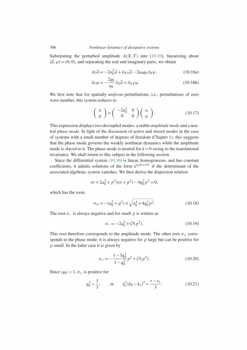
306 Nonlinear dynamics of dissipative systems

Substituting the perturbed amplitude A(X,T ) into (10.10), linearizing about(a,ϕ)= (0,0), and separating the real and imaginary parts, we obtain

∂T a =−2a20 a +∂X X a −2a0q0 ∂Xϕ, (10.16a)

∂T ϕ=−2q0

a0∂X a +∂X Xϕ. (10.16b)

We first note that for spatially uniform perturbations, i.e., perturbations of zerowave number, this system reduces to(

aϕ

)=( −2a2

0 00 0

)(aϕ

). (10.17)

This expression displays two decoupled modes: a stable amplitude mode and a neu-tral phase mode. In light of the discussion of active and slaved modes in the caseof systems with a small number of degrees of freedom (Chapter 8), this suggeststhat the phase mode governs the weakly nonlinear dynamics while the amplitudemode is slaved to it. The phase mode is neutral for k =0 owing to the translationalinvariance. We shall return to this subject in the following section.

Since the differential system (10.16) is linear, homogeneous, and has constantcoefficients, it admits solutions of the form eipX+σT if the determinant of theassociated algebraic system vanishes. We then derive the dispersion relation

(σ +2a20 + p2)(σ + p2)−4q2

0 p2 =0,

which has the roots

σ± =−(a20 + p2)±

√a4

0 +4q20 p2. (10.18)

The root σ− is always negative and for small p is written as

σ− =−2a20 +O(p2). (10.19)

This root therefore corresponds to the amplitude mode. The other root σ+ corre-sponds to the phase mode; it is always negative for p large but can be positive forp small. In the latter case it is given by

σ+ =−1−3q20

1−q20

p2 +O(p4). (10.20)

Since |q0|<1, σ+ is positive for

q20 >

1

3, or ξ2

c (k0 −kc)2 >

r −rc

3. (10.21)

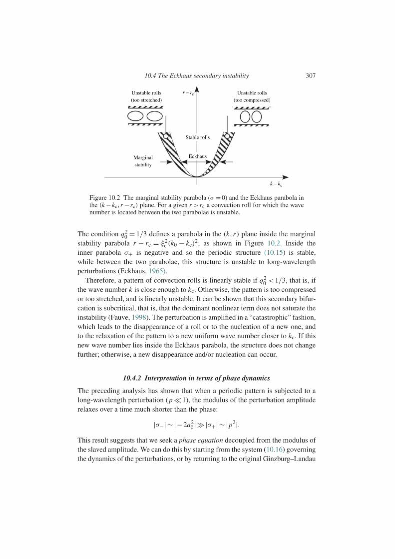
10.4 The Eckhaus secondary instability 307

Unstable rolls(too stretched)

Unstable rolls(too compressed)

Marginalstability

Eckhaus

Stable rolls

k – kc

r – rc

Figure 10.2 The marginal stability parabola (σ = 0) and the Eckhaus parabola inthe (k −kc,r −rc) plane. For a given r > rc a convection roll for which the wavenumber is located between the two parabolae is unstable.

The condition q20 = 1/3 defines a parabola in the (k,r) plane inside the marginal

stability parabola r − rc = ξ2c (k0 − kc)

2, as shown in Figure 10.2. Inside theinner parabola σ+ is negative and so the periodic structure (10.15) is stable,while between the two parabolae, this structure is unstable to long-wavelengthperturbations (Eckhaus, 1965).

Therefore, a pattern of convection rolls is linearly stable if q20 < 1/3, that is, if

the wave number k is close enough to kc. Otherwise, the pattern is too compressedor too stretched, and is linearly unstable. It can be shown that this secondary bifur-cation is subcritical, that is, that the dominant nonlinear term does not saturate theinstability (Fauve, 1998). The perturbation is amplified in a “catastrophic” fashion,which leads to the disappearance of a roll or to the nucleation of a new one, andto the relaxation of the pattern to a new uniform wave number closer to kc. If thisnew wave number lies inside the Eckhaus parabola, the structure does not changefurther; otherwise, a new disappearance and/or nucleation can occur.

10.4.2 Interpretation in terms of phase dynamics

The preceding analysis has shown that when a periodic pattern is subjected to along-wavelength perturbation (p 1), the modulus of the perturbation amplituderelaxes over a time much shorter than the phase:

|σ−|∼ |−2a20 | |σ+|∼ |p2|.

This result suggests that we seek a phase equation decoupled from the modulus ofthe slaved amplitude. We can do this by starting from the system (10.16) governingthe dynamics of the perturbations, or by returning to the original Ginzburg–Landau

308 Nonlinear dynamics of dissipative systems

equation (10.10) and separating the evolutions of the modulus and the phase ofthe envelope by introducing A = aeiφ . Choosing the second option, we obtain thecoupled equations

∂T a =(

1−(∂Xφ)2)

a +∂X X a −a3, (10.22a)

a ∂T φ=a ∂X Xφ+2∂X a ∂Xφ. (10.22b)

Rather than dealing with the actual phase φ, which increases (or decreases)spatially monotically, it is convenient to introduce the gradient of the phase

q(X,T )= ∂Xφ, (10.23)

which measures the local correction of the wave number kc to the pattern [kx =kcx +q X = (kc +εq)x]. Then, after differentiating (10.22b) with respect to X , theabove system of equations becomes

∂T a = (1−q2)a +∂X X a −a3, (10.24a)

∂T q = ∂X

(∂X q + 2q

a∂X a

). (10.24b)

This system admits a continuous family of stationary, uniform solutions

a0 =√

1−q20 , |q0|<1,

parametrized by the phase gradient q0. These solutions naturally correspond to thepattern described by (10.14) and (10.15). When one of these solutions is perturbed,the relaxation time of the perturbed amplitude a is much shorter than that of thephase gradient q, so that a remains nearly in equilibrium with q, i.e., it is given bya2 = 1−q2 (a is said to follow q “adiabatically” or to be “slaved” to q). We thenfind that ∂X a = (−q/a)∂X q. Inserting this expression into (10.24b), we obtain

∂T q = ∂X (D(q)∂X q) , D(q)= 1−3q2

1−q2. (10.25)

This is a nonlinear diffusion equation involving a diffusivity D(q). Linearizing theequation for small perturbations δq =q −q0, we find

∂T δq = D(q0)∂X Xδq. (10.26)

For q20 < 1/3 the diffusivity D(q0) is positive and the wave number q relaxes to

equilibrium q0; otherwise, the diffusivity D(q0) is negative and the local wavenumber diverges. We therefore arrive at the Eckhaus instability criterion (10.21)from the point of view of phase dynamics.

10.4 The Eckhaus secondary instability 309

A weakly nonlinear expansion of the phase equation near the Eckhaus instabilityleads to an equation of the Kuramoto–Sivashinsky type, in which the nonlinearterm is such that the bifurcation is subcritical, as mentioned above (Kuramoto,1984; Fauve, 1998, §6). The idea of phase dynamics, introduced by Pomeau andManneville (1979), has proved to be very fruitful. Beyond the weakly nonlinearregime, it led to the introduction of the concept of “phase turbulence” to analyzechaotic behaviors (Manneville, 1990, chapter 10).

10.4.3 Some experimental illustrations

Two physical systems corresponding to the above situation have been studiedextensively: the Rayleigh–Benard convection between two horizontal plates andthe Couette–Taylor flow between two cylinders. A review is given in the books ofKoschmieder (1993) and Chossat and Iooss (1994). These studies reveal generictypes of behavior that must occur in any system possessing the same symme-tries, that is, in any system invariant under the reflectional and translationalsymmetries.

In the case of Rayleigh–Benard convection, the observed spatial patterns dependon the shape and size of the box, on the type of wall (whether it imposes a temper-ature or a thermal flux), and on the Prandtl number Pr = ν/κ , where ν and κ arethe kinematic viscosity and thermal diffusivity of the fluid. These patterns can bealigned rolls, or two-dimensional rectangular or hexagonal structures (Manneville,1990, chapter 4). In the case of rolls, the Eckhaus secondary instability is man-ifested as a local compression (stretching) of the initial pattern, which typicallyleads to the disappearance (appearance) of rolls and the relaxation of the systemto a larger (smaller) wavelength. Figure 10.3 illustrates a particular manifestationof the Eckhaus instability, the cross-roll instability (Busse and Whitehead, 1971).The initial pattern is imposed by a thermal impression technique, which consistsof gently heating the fluid just below the critical Rayleigh number Rac using alamp shining through a grill. The illuminated regions are warmer than the onesin the shadow of the grill, and a forced convection motion arises. Upon passingthrough Rac and suppressing the forcing, the initial rolls (top left panel) are unsta-ble because they are too compressed; a system of rolls with a larger wavelengthand orthogonal to the original ones develops and tends to replace them, as seen inthe bottom right panel.

Another variant of the Eckhaus instability is the zigzag instability, illustrated inFigure 10.4. Here the initial rolls, shown in the top left panel, are too stretched,and the appearance of the zigzags (bottom right panel) is an economical way oflocally reducing the wavelength via small perturbations, that is, without the needto create new rolls.

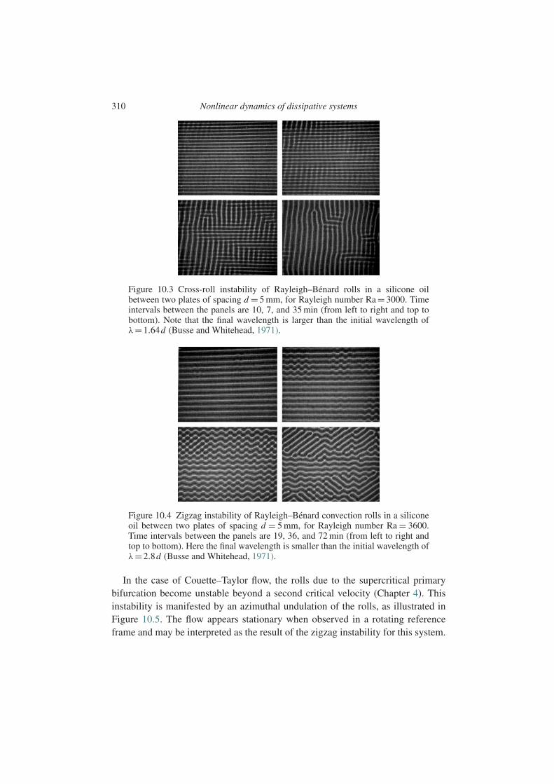
310 Nonlinear dynamics of dissipative systems

Figure 10.3 Cross-roll instability of Rayleigh–Benard rolls in a silicone oilbetween two plates of spacing d = 5 mm, for Rayleigh number Ra = 3000. Timeintervals between the panels are 10, 7, and 35 min (from left to right and top tobottom). Note that the final wavelength is larger than the initial wavelength ofλ=1.64d (Busse and Whitehead, 1971).

Figure 10.4 Zigzag instability of Rayleigh–Benard convection rolls in a siliconeoil between two plates of spacing d = 5 mm, for Rayleigh number Ra = 3600.Time intervals between the panels are 19, 36, and 72 min (from left to right andtop to bottom). Here the final wavelength is smaller than the initial wavelength ofλ=2.8d (Busse and Whitehead, 1971).

In the case of Couette–Taylor flow, the rolls due to the supercritical primarybifurcation become unstable beyond a second critical velocity (Chapter 4). Thisinstability is manifested by an azimuthal undulation of the rolls, as illustrated inFigure 10.5. The flow appears stationary when observed in a rotating referenceframe and may be interpreted as the result of the zigzag instability for this system.

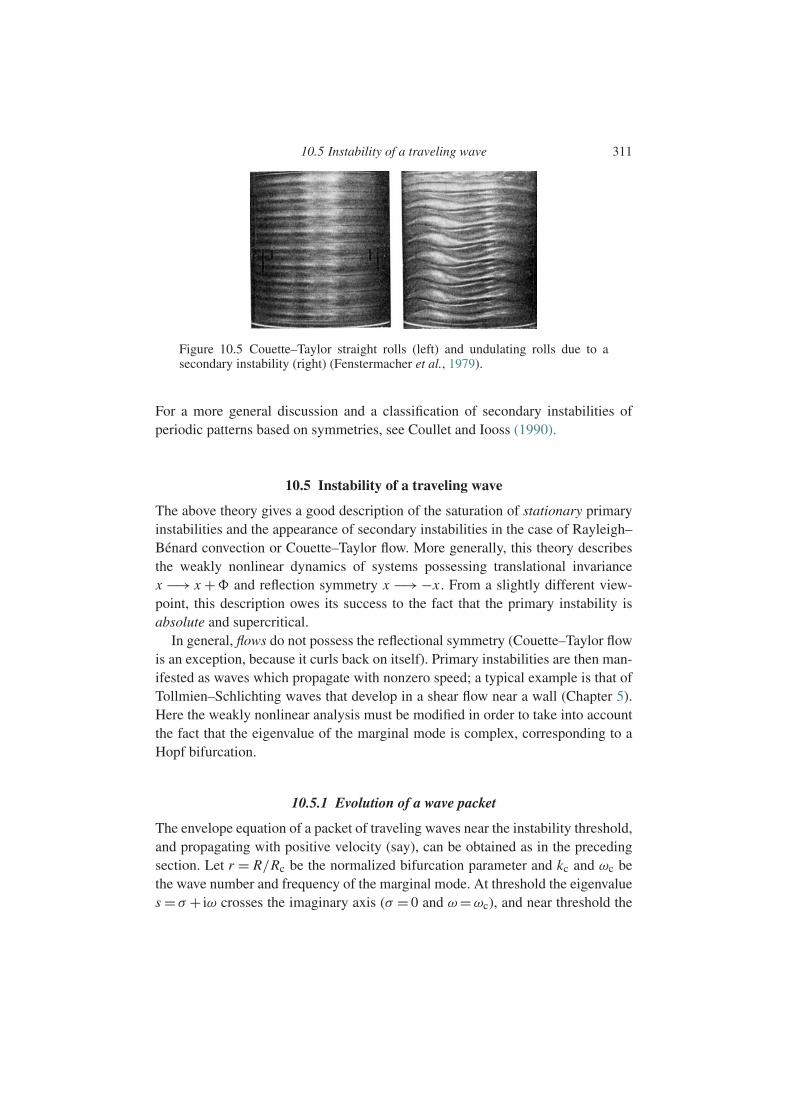
10.5 Instability of a traveling wave 311

Figure 10.5 Couette–Taylor straight rolls (left) and undulating rolls due to asecondary instability (right) (Fenstermacher et al., 1979).

For a more general discussion and a classification of secondary instabilities ofperiodic patterns based on symmetries, see Coullet and Iooss (1990).

10.5 Instability of a traveling wave

The above theory gives a good description of the saturation of stationary primaryinstabilities and the appearance of secondary instabilities in the case of Rayleigh–Benard convection or Couette–Taylor flow. More generally, this theory describesthe weakly nonlinear dynamics of systems possessing translational invariancex −→ x + and reflection symmetry x −→ −x . From a slightly different view-point, this description owes its success to the fact that the primary instability isabsolute and supercritical.

In general, flows do not possess the reflectional symmetry (Couette–Taylor flowis an exception, because it curls back on itself). Primary instabilities are then man-ifested as waves which propagate with nonzero speed; a typical example is that ofTollmien–Schlichting waves that develop in a shear flow near a wall (Chapter 5).Here the weakly nonlinear analysis must be modified in order to take into accountthe fact that the eigenvalue of the marginal mode is complex, corresponding to aHopf bifurcation.

10.5.1 Evolution of a wave packet

The envelope equation of a packet of traveling waves near the instability threshold,and propagating with positive velocity (say), can be obtained as in the precedingsection. Let r = R/Rc be the normalized bifurcation parameter and kc and ωc bethe wave number and frequency of the marginal mode. At threshold the eigenvalues = σ + iω crosses the imaginary axis (σ = 0 and ω=ωc), and near threshold the

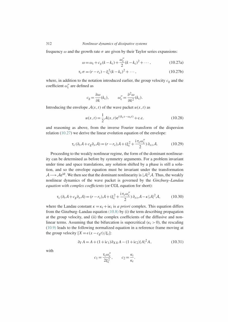
312 Nonlinear dynamics of dissipative systems

frequency ω and the growth rate σ are given by their Taylor series expansions:

ω=ωc +cg(k −kc)+ ω′′c

2(k −kc)

2 + ·· · , (10.27a)

τc σ = (r −rc)−ξ2c (k −kc)

2 + ·· · , (10.27b)

where, in addition to the notation introduced earlier, the group velocity cg and thecoefficient ω′′

c are defined as

cg = ∂ω

∂k(kc), ω′′

c = ∂2ω

∂k2(kc).

Introducing the envelope A(x, t) of the wave packet u(x, t) as

u(x, t)= 1

2A(x, t)ei(kcx−ωct)+c.c. (10.28)

and reasoning as above, from the inverse Fourier transform of the dispersionrelation (10.27) we derive the linear evolution equation of the envelope:

τc (∂tA+cg∂xA)= (r −rc)A+(ξ2c + iτcω

′′c

2)∂xxA. (10.29)

Proceeding to the weakly nonlinear regime, the form of the dominant nonlinear-ity can be determined as before by symmetry arguments. For a problem invariantunder time and space translations, any solution shifted by a phase is still a solu-tion, and so the envelope equation must be invariant under the transformationA−→Aeiφ . We then see that the dominant nonlinearity is |A|2A. Thus, the weaklynonlinear dynamics of the wave packet is governed by the Ginzburg–Landauequation with complex coefficients (or CGL equation for short):

τc (∂tA+cg∂xA)= (r −rc)A+(ξ2c + iτcω

′′c

2)∂xxA−κ|A|2A, (10.30)

where the Landau constant κ = κr + iκi is a priori complex. This equation differsfrom the Ginzburg–Landau equation (10.8) by (i) the term describing propagationat the group velocity, and (ii) the complex coefficients of the diffusive and non-linear terms. Assuming that the bifurcation is supercritical (κr > 0), the rescaling(10.9) leads to the following normalized equation in a reference frame moving atthe group velocity [X = ε(x −cgt)/ξc]:

∂T A = A+(1+ ic1)∂X X A−(1+ ic2)|A|2 A, (10.31)

with

c1 = τcω′′c

2ξ2c

, c2 = κi

κr.

10.5 Instability of a traveling wave 313

As we shall see, solutions and their stability are governed by the parameters c1

and c2.

10.5.2 A nonlinear wave

The complex Ginzburg–Landau equation (10.31) admits the family of solutions

A0(X,T )=a0 ei(q0 X−T +), (10.32a)

a0 =√

1−q20 , (10.32b)

= c2 +(c1 −c2)q20 , (10.32c)

parametrized by q0 spanning the interval [−1,1], where is an undeterminedphase reflecting the translational invariance of the problem. These solutionscorrespond to traveling waves

U0(x, t)=u0 cos(k0x −ω0t +), (10.33)

with amplitude, wave number, and frequency given by

u0 =√r −rc

√1−q2

0

κ, (10.34a)

k0 = kc + q0√

r −rc

ξc, (10.34b)

ω0 =ω#+ 1

τcκiu

20 with ω# =ωc +cg(k0 −kc)+ ω′′

c

2(k0 −kc)

2. (10.34c)

The frequency is therefore the sum of the frequency ω# of waves of infinitesi-mal amplitude (where the subscript # refers to the result (10.27a) of the linearanalysis) and a finite-amplitude correction proportional to κi. We note that theamplitude and wave number are identical to those of the solutions (10.15) ofthe Ginzburg–Landau equation with real coefficients, and that the frequency cor-rection is identical to the Stokes correction of a dispersive wave introduced inChapter 9.

Like the Ginzburg–Landau equation with real coefficients and the nonlinearSchrodinger equation, the complex Ginzburg–Landau equation admits localizedsolutions (Cross and Hohenberg, 1993; Fauve, 1998) which we do not discuss here.

10.5.3 The Benjamin–Feir–Eckhaus instability

The stability analysis of the nonlinear wave (10.33) goes along the same linesas that of the stationary pattern (10.15) governed by the real Ginzburg–Landau

314 Nonlinear dynamics of dissipative systems

equation. Perturbing the amplitude and phase of the envelope (10.32) as

A(X,T )= [a0 + a(X,T )]ei[q0 X−T++ϕ(X,T )],

substituing this expression into the CGL equation, and linearizing for small dis-turbances, we obtain a system similar to (10.16). The dispersion relation is thenobtained by expressing the solution in the form of normal modes. As before, thisanalysis reveals a strongly damped amplitude mode as well as a weakly damped oramplified phase mode in the limit of perturbations with zero wave number (relatedto the translational invariance). The instability criterion emerges clearly when westudy the equation for the phase perturbation ϕ(X,T ). In the long-wavelength limitthis equation is a diffusion equation with diffusion coefficient (Kuramoto, 1984;Janiaud et al., 1992)

D(q0)=1+c1c2 − 2q20 (1+c2

2)

1−q20

. (10.35)

From this expression we deduce the following results, which are summarized inFigure 10.6 showing the various cases in the (c1,c2) plane:

• For 1+ c1c2 > 0, i.e., between the two branches of the hyperbola 1+ c1c2 = 0shown in Figure 10.6, there exist stable waves of finite amplitude among all

Benjamin–Feir

Benjamin–Feir

Eckhaus

r – rc

r – rc r – rc

r – rc

k – kc

k – kc k – kc

k – kc

c2

c1

Figure 10.6 Domain where unstable waves exist (shaded region) in the (k −kc,r −rc) plane, depending on whether the point (c1,c2) is outside or inside thehyperbola of Lange and Newell.

10.5 Instability of a traveling wave 315

the waves existing for r − rc > ξ2c (k − kc)

2 (i.e., inside the marginal stabilityparabola) such that the parameter q0 satisfies the condition

q20 <

1+c1c2

2(1+c22)+1+c1c2

. (10.36)

For c1 =c2 =0 we recover the Eckhaus criterion (10.21) (since the CGL equationthen has real coefficients). For nonzero c1 and c2 the width of the band of stablewave numbers depends on c1 and c2, and vanishes on the hyperbola.

• For 1+ c1c2 < 0, i.e., outside the two branches of the hyperbola 1 + c1c2 = 0,the diffusion coefficient is negative for all q0 lying between −1 and +1, andnone of the finite-amplitude waves (10.15) is stable (Lange and Newell, 1974).For large c2 = −c1 the coefficients of the diffusive and nonlinear terms of theCGL equation are essentially imaginary, and the CGL equation degenerates intoa nonlinear Schrodinger equation: the wave instability therefore corresponds tothe Benjamin–Feir instability discussed in the preceding chapter.

Therefore, the Eckhaus and Benjamin–Feir instabilities are unified in the for-malism of envelope equations. This kinship of the two instabilities was noticed byStuart and DiPrima (1978), who showed, by perturbing a finite-amplitude waveby a sum of two nearby wave numbers, that the Eckhaus instability can be inter-preted in terms of resonant interactions, as in the Benjamin–Feir instability. (Inthe Eckhaus case there is only the resonance condition on the wave numbers; theresonance condition on the frequencies is degenerate as all the frequencies arezero.)

10.5.4 Tollmien–Schlichting waves and the transition to turbulence

With the above results on the stability of nonlinear traveling waves in mind, wenow return to the problem of the stability of parallel flows U (y). As discussed inChapter 5, plane Poiseuille flow is linearly unstable beyond the critical Reynoldsnumber Rec = 5772 with marginal wave number kch = 1.02. Stewartson and Stu-art (1971) have shown that near this threshold the weakly nonlinear dynamics areeffectively governed by the Ginzburg–Landau equation (10.30), with negative realpart of the Landau coefficient: the Hopf bifurcation is subcritical. The cubic non-linearity does not saturate the primary instability, but instead further amplifies theperturbation (Drazin, 2002, §5.2 and §8.9).

The search for finite-amplitude bifurcated branches requires numerical compu-tation. These computations show that there exists a nonlinear neutral surface inthe (Re, kh, E) parameter space, where E is the disturbance energy of the wave(see references in Bayly et al. (1988)). Two sections of this surface are shown

316 Nonlinear dynamics of dissipative systems

kh = 1.32

kh = 1.02

2900

E

5772 Re

Figure 10.7 Bifurcation diagram for plane Poiseuille flow for two-dimensionalperturbations with energy E , for kch =1.02 and 1.32; (—), stable branches; (– –),unstable branches.

in Figure 10.7 for fixed wave numbers. The section for the critical wave numberkch = 1.02 shows the branch of unstable waves which arises from the subcriticalHopf bifurcation, and merges with a stable branch at a Reynolds number approx-imately equal to 4600 (the merging corresponding to a saddle–node bifurcation).The second section is for wave number kh = 1.32: although this wave number islinearly unstable for any Reynolds number, there exist two branches of finite ampli-tude waves, one unstable and the other stable, which merge for Reg ≈2900. Belowthis Reynolds number the flow is globally stable, that is, it relaxes to Poiseuilleflow for initial two-dimensional perturbations of arbitrary amplitude (Chapter 3).More general solutions, such as three-dimensional waves, are however found toexist for Reynolds number even below Reg (Ehrenstein and Koch, 1991; Huerreand Rossi, 1998).

In spite of the subcritical nature of the bifurcation, secondary instabilities offorced Tollmien–Schlichting waves have been observed before the transition toturbulence. For example, in the case of boundary layer flow, Klebanoff et al.(1962) observed that beyond a certain distance downstream a spanwise (along thez-direction) undulation of the wave crests with a well-defined wavelength λz

appears. Two successive crests are typically out of phase by λz/4 and form an alter-nating “$” pattern. These observations stimulated further analysis, which revealedtwo secondary instability mechanisms of two-dimensional waves: an ellipticalmechanism and a subharmonic mechanism (see the reviews by Bayly et al. (1988);Herbert (1988); Huerre and Rossi (1998, §8); and Kerswell (2002)). Both of theseinstabilities are inviscid and therefore develop over a time of the order of theinverse of the velocity gradient, U

′(y), which is much shorter than the time scale

of the primary (viscous) instability, which in turn is why they can be observed.However, the diagram in Figure 10.7, along with the observations briefly sum-

marized above regarding secondary instabilities, are not at all the last word on thestability of Poiseuille flow or boundary layer flow. Importantly, as discussed in

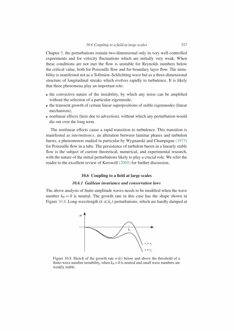
10.6 Coupling to a field at large scales 317

Chapter 5, the perturbations remain two-dimensional only in very well-controlledexperiments and for velocity fluctuations which are initially very weak. Whenthese conditions are not met the flow is unstable for Reynolds numbers belowthe critical value, both for Poiseuille flow and for boundary layer flow. The insta-bility is manifested not as a Tollmien–Schlichting wave but as a three-dimensionalstructure of longitudinal streaks which evolves rapidly to turbulence. It is likelythat three phenomena play an important role:

• the convective nature of the instability, by which any noise can be amplifiedwithout the selection of a particular eigenmode;

• the transient growth of certain linear superpositions of stable eigenmodes (linearmechanism);

• nonlinear effects (here due to advection), without which any perturbation woulddie out over the long term.

The nonlinear effects cause a rapid transition to turbulence. This transition ismanifested as intermittency, an alteration between laminar phases and turbulentbursts, a phenomenon studied in particular by Wygnanski and Champagne (1973)for Poiseuille flow in a tube. The persistence of turbulent bursts in a linearly stableflow is the subject of current theoretical, numerical, and experimental research,with the nature of the initial perturbations likely to play a crucial role. We refer thereader to the excellent review of Kerswell (2005) for further discussion.

10.6 Coupling to a field at large scales

10.6.1 Galilean invariance and conservation laws

The above analysis of finite-amplitude waves needs to be modified when the wavenumber k0 = 0 is neutral. The growth rate in this case has the shape shown inFigure 10.8. Long-wavelength (k kc) perturbations, which are hardly damped at

kc

σ

r > rc

r < rc

Figure 10.8 Sketch of the growth rate σ(k) below and above the threshold of afinite-wave number instability, when k0 =0 is neutral and small wave numbers areweakly stable.

318 Nonlinear dynamics of dissipative systems

all, can easily be excited by a linearly unstable mode of finite wave number kc. Thecoupling of the two modes then leads to new dynamics.

This situation arises, in particular, when the problem satisfies Galilean invari-ance, that is, invariance under the transformation

y = x −V t, v=u −V . (10.37)

As an example, let us consider the model equation

∂t u = Lu −u∂x u, L = ∂2x +2r∂4

x +∂6x . (10.38)

We note first of all that this equation is translationally invariant: if u(x, t) is a solu-tion, it is easily checked that the function v(x, t)= u(x −φ, t), corresponding tou(x, t) translated by a phase φ, is also a solution. As discussed in Section 10.4, thistranslational invariance is associated with a neutral phase mode. Equation (10.38)also satisfies Galilean invariance; indeed, under the Galilean transformation y =x −V t it becomes

∂t u = ∂2y u +2r∂4

y u +∂6y u −(u −V )∂yu,

and it can be verified that the transformation v=u −V restores Eq. (10.37).2

In hydrodynamics, Galilean invariance is generally broken by the no-slipcondition at the walls, but it can survive in certain cases, for example, in Rayleigh–Benard convection with free boundaries. It is also possible to have approximateGalilean invariance, for example, in Rayleigh–Benard convection with fixedboundaries but small Prandtl number (which for low viscosity results in thin veloc-ity boundary layers on the upper and lower walls). Far from the lateral walls, aslow horizontal flow at large scales has almost no dissipation, which correspondsto nearly neutral perturbations of very small wave number (Siggia and Zippelius,1981).

The situation of neutral zero wave number is also encountered when theevolution equation can be written in the form of a conservation law:

∂tU +∂x [ f (U,∂xU, ...)]=0, (10.39)

where the function f is a sum of products of U and its derivatives. A perturbationu ei(kx−ωt)+c.c. of a stationary, uniform solution U0 of this equation satisfies thedispersion relation

−iω+ ik f ′(U0)+O(k2)=0, (10.40)

2 As a counter-example, it can be checked that the Swift–Hohenberg equation (10.13) is not Galilean-invariant.

10.6 Coupling to a field at large scales 319

which clearly shows that the k =0 mode is neutral. This is the case in thermohalineconvection, where U (x, t) is the salt concentration field (Riecke, 1992). Anotherexample is a flow of finite depth with a free surface.3 In this case the field U (x, t)represents the thickness of the fluid layer, f (U,∂xU, ...) is the horizontal flow rate,and the mass conservation is expressed by a law of the type (10.39) (Renardy andRenardy, 1993).

10.6.2 Coupled evolution equations

Let us consider a perturbation of a stationary, uniform base flow near the marginalstability r = rc in the form of the sum

u(x, t)= 1

2A(x, t)ei(kcx−ωct)+c.c.+B(x, t). (10.41)

Here A(x, t) is the complex envelope of a wave packet centered on the finite wavenumber kc and B(x, t) represents the (real) long-wavelength perturbation, which isnearly neutral.

Neglecting for the moment the coupling between A and B, the weakly nonlinearevolution of the envelope A is, as before, governed by the complex Ginzburg–Landau equation (10.30). The linear evolution equation of the mode B is obtainedfrom a Taylor series expansion of the dispersion relation about k0 =0, or

∂tB=−c0∂xB+ ξ20

τc∂xxB, (10.42)

where the speed c0 and the diffusion length ξ0 of the k0 =0 mode are defined as

c0 = ∂ω

∂k,

ξ20

τc=−1

2

∂2σ

∂k2,

with the derivatives evaluated at the critical point (rc = 1,k0 = 0). The dif-fusion coefficient ξ2

0 /τc is positive for linearly stable, long-wavelength wavescorresponding to Figure 10.8.

The determination of the dominant coupling terms depends on the choice of therelative order of magnitude of A and B. Since experiment shows that B is small

3 We note that the weakly nonlinear stability of a liquid film falling down an inclined plane is not described bythis analysis. In fact, the linear analysis shows that the instability does not arise on a mode of isolated finitewave number, but instead occurs on an unstable band extending from k = 0 to the cutoff wave number (long-wave instability); see Chapter 6 and also Ruyer-Quil and Manneville (2000) and Chang (1994). The analysis ofBenney (1966), which considers the interaction of a harmonic k0 with the average flow (k = 0) and the secondharmonic 2k0, leads to a CGL equation, but this analysis is incomplete as it ignores the continuous nature ofthe spectrum of unstable wave numbers.

320 Nonlinear dynamics of dissipative systems

compared to |A|, we can take

B∼ εA∼ ε2.

The dominant coupling terms satisfying translational invariance are then AB inthe equation for A, and ∂x |A|2 in the equation for B (since the latter term is largerby at least one order of magnitude compared to nonlinear terms involving only B).Finally, the change of scale (10.9) leads, in a reference frame moving at the groupvelocity cg(kc), to the following system of coupled equations:

∂T A = A+(1+ ic1)∂X X A−(1+ ic2)|A|2 A+(1+ ic3)AB, (10.43a)

∂T B = ε−1τc

ξc(cg −c0)∂X B + ξ2

0

ξ2c∂X X B +ε−1γ ∂X |A|2, (10.43b)

where the mode B has been scaled such that the coefficient of the coupling termAB is normalized to 1+ ic3. This equation describes, for example, the evolution ofthe interface between two layers of viscous fluids in Couette–Poiseuille flow: thecoefficients for this case have been calculated by Renardy and Renardy (1993).

Therefore, all the terms in the equation for A are of the same order of magnitude(ε3), but this is not the case in the equation for B. If the coefficients τc(cg −c0)/ξc

and γ are of order unity, Eq. (10.43b) becomes degenerate and can be integratedto give

B = ξcγ

τc(cg −c0)|A|2.

The mode B is therefore slaved to A and does not bring in anything qualitativelynew. However, the situation is changed if the difference cg − c0 and the couplingcoefficient γ are small, of order ε: in this case the four terms of Eq. (10.43b) arethen all of the same order of magnitude. It is this situation that we shall studybelow.

We note that in the case of a stationary bifurcation (ωc =0), a similar system ofamplitude equations which also possesses reflection symmetry x −→−x has beenstudied by Coullet and Fauve (1985).

10.6.3 Wave stability

The system (10.43) admits the family of solutions B0 = 0 and A0 given byEq. (10.32), which corresponds to the finite-amplitude waves (10.33). The stabilityof these waves has been studied by Barthelet and Charru (1998), and here we onlyquote the main results. For spatially uniform perturbations, i.e., perturbations with

10.6 Coupling to a field at large scales 321

Unstable waves Stable waves

Marginalstability

r – rc

k – kc

Figure 10.9 Marginal stability parabola in the (k − kc, r − rc) plane and theparabolae bounding the regions where stable and unstable waves exist (white andhatched regions, respectively).

zero wave number, the system of equations for the perturbations reduces to aϕ

b

= −2a2

0 0 1−2a0c1 0 c3

0 0 0

aϕ

b

, (10.44)

which has the eigenvalues

s1 =−2a20, s2 =0, s3 =0.

We recover the stable amplitude mode and the two neutral modes correspondingto the two invariances, translational and Galilean (we note that this matrix can bediagonalized by a change of variables for A and B corresponding to a rotationin the complex plane). For spatially periodic rather than uniform perturbations,it can be shown from the dispersion relation that there are stable waves inside themarginal stability parabola in the (k, r ) plane, i.e. in the lenticular regions boundedby arcs of parabolae, as shown in Figure 10.9. These arcs are not symmetricabout the k = kc axis, which is consistent with the absence of reflection symme-try. Finally, the coupling to a long-wavelength mode has the effect of breaking theEckhaus parabola (10.21) into several arcs.

10.6.4 An experimental illustration

The results of this analysis can be illustrated by observations of the secondaryinstability of waves at the interface between two superposed sheared liquids(Charru and Barthelet, 1999). The experiment, already described in Chapter 8,consists of an annular channel of perimeter L with a rotating upper plate whichsets the fluids in motion. For certain viscosity ratios a wave of wavelength 2π/kon the centimeter scale appears at the interface above a critical speed Uc of the

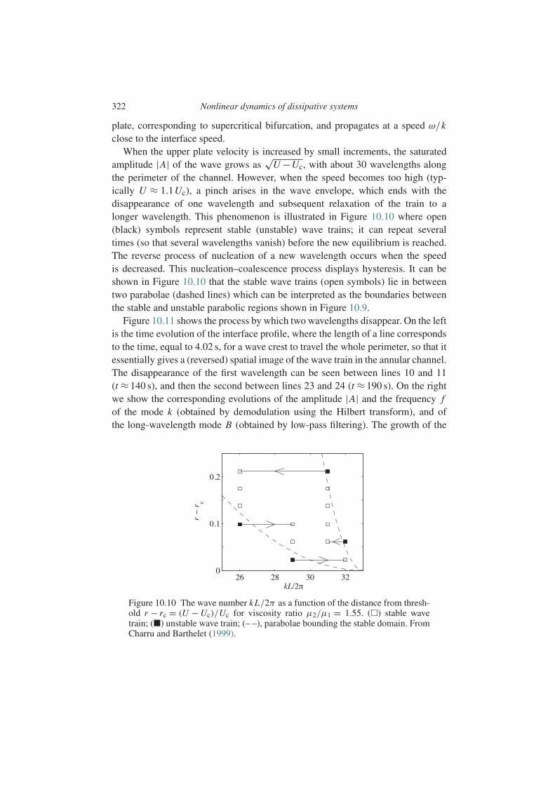
322 Nonlinear dynamics of dissipative systems

plate, corresponding to supercritical bifurcation, and propagates at a speed ω/kclose to the interface speed.

When the upper plate velocity is increased by small increments, the saturatedamplitude |A| of the wave grows as

√U −Uc, with about 30 wavelengths along

the perimeter of the channel. However, when the speed becomes too high (typ-ically U ≈ 1.1Uc), a pinch arises in the wave envelope, which ends with thedisappearance of one wavelength and subsequent relaxation of the train to alonger wavelength. This phenomenon is illustrated in Figure 10.10 where open(black) symbols represent stable (unstable) wave trains; it can repeat severaltimes (so that several wavelengths vanish) before the new equilibrium is reached.The reverse process of nucleation of a new wavelength occurs when the speedis decreased. This nucleation–coalescence process displays hysteresis. It can beshown in Figure 10.10 that the stable wave trains (open symbols) lie in betweentwo parabolae (dashed lines) which can be interpreted as the boundaries betweenthe stable and unstable parabolic regions shown in Figure 10.9.

Figure 10.11 shows the process by which two wavelengths disappear. On the leftis the time evolution of the interface profile, where the length of a line correspondsto the time, equal to 4.02 s, for a wave crest to travel the whole perimeter, so that itessentially gives a (reversed) spatial image of the wave train in the annular channel.The disappearance of the first wavelength can be seen between lines 10 and 11(t ≈ 140 s), and then the second between lines 23 and 24 (t ≈ 190 s). On the rightwe show the corresponding evolutions of the amplitude |A| and the frequency fof the mode k (obtained by demodulation using the Hilbert transform), and ofthe long-wavelength mode B (obtained by low-pass filtering). The growth of the

Figure 10.10 The wave number kL/2π as a function of the distance from thresh-old r − rc = (U − Uc)/Uc for viscosity ratio µ2/µ1 = 1.55. () stable wavetrain; () unstable wave train; (– –), parabolae bounding the stable domain. FromCharru and Barthelet (1999).

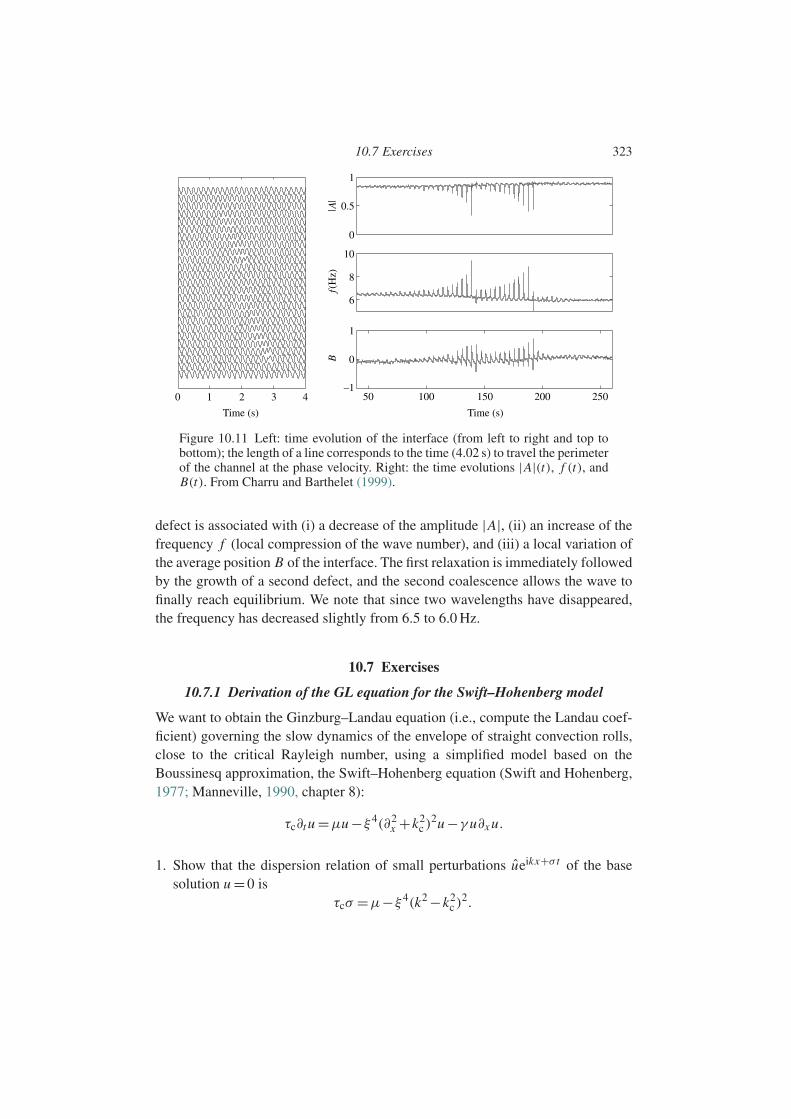
10.7 Exercises 323

50

1

0.5A

f(H

z)B

0

10

8

6

1

0

–1100 150 200 250

Time (s)Time (s)

0 1 2 3 4

Figure 10.11 Left: time evolution of the interface (from left to right and top tobottom); the length of a line corresponds to the time (4.02 s) to travel the perimeterof the channel at the phase velocity. Right: the time evolutions |A|(t), f (t), andB(t). From Charru and Barthelet (1999).

defect is associated with (i) a decrease of the amplitude |A|, (ii) an increase of thefrequency f (local compression of the wave number), and (iii) a local variation ofthe average position B of the interface. The first relaxation is immediately followedby the growth of a second defect, and the second coalescence allows the wave tofinally reach equilibrium. We note that since two wavelengths have disappeared,the frequency has decreased slightly from 6.5 to 6.0 Hz.

10.7 Exercises

10.7.1 Derivation of the GL equation for the Swift–Hohenberg model

We want to obtain the Ginzburg–Landau equation (i.e., compute the Landau coef-ficient) governing the slow dynamics of the envelope of straight convection rolls,close to the critical Rayleigh number, using a simplified model based on theBoussinesq approximation, the Swift–Hohenberg equation (Swift and Hohenberg,1977; Manneville, 1990, chapter 8):

τc∂t u =µu −ξ4(∂2x +k2

c )2u −γ u∂x u.

1. Show that the dispersion relation of small perturbations ueikx+σ t of the basesolution u =0 is

τcσ =µ−ξ4(k2 −k2c )

2.

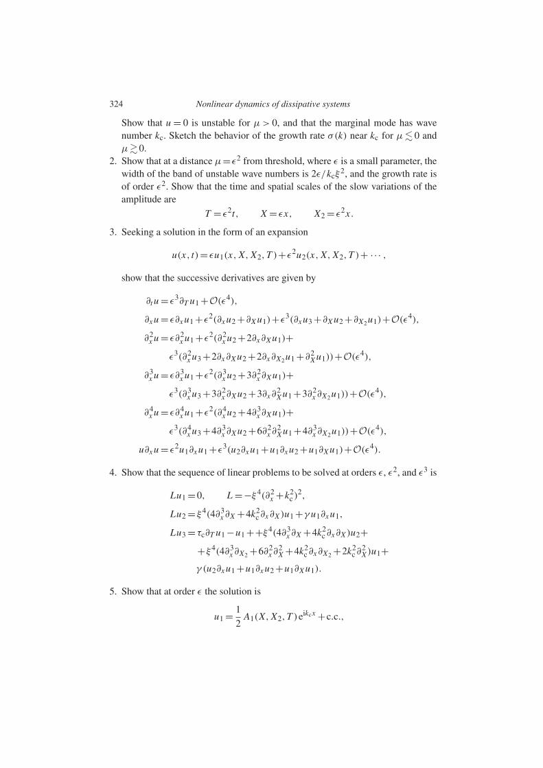
324 Nonlinear dynamics of dissipative systems

Show that u = 0 is unstable for µ> 0, and that the marginal mode has wavenumber kc. Sketch the behavior of the growth rate σ(k) near kc for µ 0 andµ0.

2. Show that at a distance µ=ε2 from threshold, where ε is a small parameter, thewidth of the band of unstable wave numbers is 2ε/kcξ

2, and the growth rate isof order ε2. Show that the time and spatial scales of the slow variations of theamplitude are

T = ε2t, X = εx, X2 = ε2x .

3. Seeking a solution in the form of an expansion

u(x, t)= εu1(x, X, X2,T )+ε2u2(x, X, X2,T )+ ·· · ,

show that the successive derivatives are given by

∂t u = ε3∂T u1 +O(ε4),

∂x u = ε∂x u1 +ε2(∂x u2 +∂X u1)+ε3(∂x u3 +∂X u2 +∂X2u1)+O(ε4),

∂2x u = ε∂2

x u1 +ε2(∂2x u2 +2∂x∂X u1)+

ε3(∂2x u3 +2∂x∂X u2 +2∂x∂X2u1 +∂2

X u1))+O(ε4),

∂3x u = ε∂3

x u1 +ε2(∂3x u2 +3∂2

x ∂X u1)+ε3(∂3

x u3 +3∂2x ∂X u2 +3∂x∂

2X u1 +3∂2

x ∂X2u1))+O(ε4),

∂4x u = ε∂4

x u1 +ε2(∂4x u2 +4∂3

x ∂X u1)+ε3(∂4

x u3 +4∂3x ∂X u2 +6∂2

x ∂2X u1 +4∂3

x ∂X2u1))+O(ε4),

u∂x u = ε2u1∂x u1 +ε3(u2∂x u1 +u1∂x u2 +u1∂X u1)+O(ε4).

4. Show that the sequence of linear problems to be solved at orders ε, ε2, and ε3 is

Lu1 =0, L =−ξ4(∂2x +k2

c )2,

Lu2 = ξ4(4∂3x ∂X +4k2

c∂x∂X )u1 +γ u1∂x u1,

Lu3 = τc∂T u1 −u1 ++ξ4(4∂3x ∂X +4k2

c∂x∂X )u2++ξ4(4∂3

x ∂X2 +6∂2x ∂

2X +4k2

c∂x∂X2 +2k2c∂

2X )u1+

γ (u2∂x u1 +u1∂x u2 +u1∂X u1).

5. Show that at order ε the solution is

u1 = 1

2A1(X, X2,T )eikcx +c.c.,

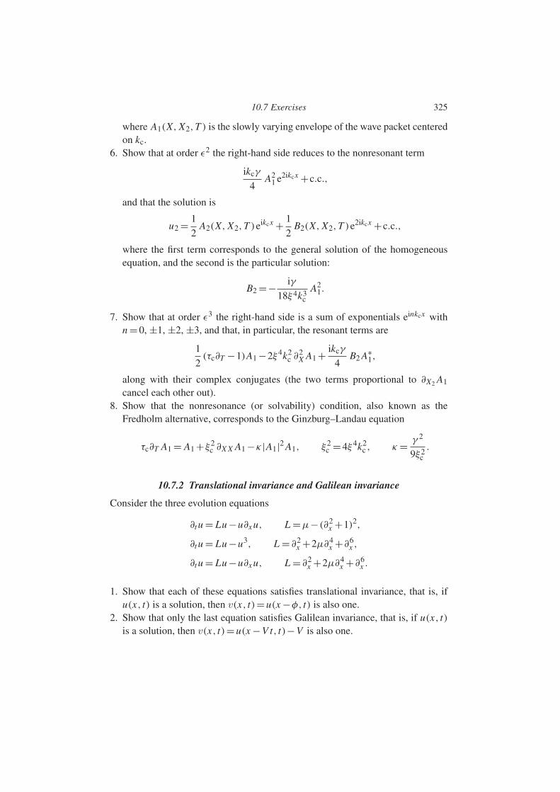
10.7 Exercises 325

where A1(X, X2,T ) is the slowly varying envelope of the wave packet centeredon kc.

6. Show that at order ε2 the right-hand side reduces to the nonresonant term

ikcγ

4A2

1 e2ikcx +c.c.,

and that the solution is

u2 = 1

2A2(X, X2,T )eikcx + 1

2B2(X, X2,T )e2ikcx +c.c.,

where the first term corresponds to the general solution of the homogeneousequation, and the second is the particular solution:

B2 =− iγ

18ξ4k3c

A21.

7. Show that at order ε3 the right-hand side is a sum of exponentials einkcx withn =0, ±1, ±2, ±3, and that, in particular, the resonant terms are

1

2(τc∂T −1)A1 −2ξ4k2

c ∂2X A1 + ikcγ

4B2 A∗

1,

along with their complex conjugates (the two terms proportional to ∂X2 A1

cancel each other out).8. Show that the nonresonance (or solvability) condition, also known as the

Fredholm alternative, corresponds to the Ginzburg–Landau equation

τc∂T A1 = A1 +ξ2c ∂X X A1 −κ|A1|2 A1, ξ2

c =4ξ4k2c , κ = γ 2

9ξ2c.

10.7.2 Translational invariance and Galilean invariance

Consider the three evolution equations

∂t u = Lu −u∂x u, L =µ−(∂2x +1)2,

∂t u = Lu −u3, L = ∂2x +2µ∂4

x +∂6x ,

∂t u = Lu −u∂x u, L = ∂2x +2µ∂4

x +∂6x .

1. Show that each of these equations satisfies translational invariance, that is, ifu(x, t) is a solution, then v(x, t)=u(x −φ, t) is also one.

2. Show that only the last equation satisfies Galilean invariance, that is, if u(x, t)is a solution, then v(x, t)=u(x −V t, t)−V is also one.

11

Dynamical systems and bifurcations

11.1 Introduction

A useful mathematical framework for studying linear and nonlinear stability isthe theory of ordinary differential equations (ODEs), also known as the theory ofdynamical systems when the focus is on geometric and qualitative representationsof the ideas and solutions. An informal presentation of this theory was given inChapter 1. The goal of this chapter is to give a more systematic account of it from amathematical point of view. In particular, we shall show how to reduce the numberof degrees of freedom of a problem to obtain the “normal forms” of elementarybifurcations referred to often in the previous chapters.

In spite of its restrictive nature relative to the theory of partial differentialequations, the theory of dynamical systems has revealed the extraordinary rich-ness and complexity of the types of behavior that can arise when nonlinear effectsplay a role. This theory originated in the work of Henri Poincare, in particular, inhis book Methodes nouvelles de la mecanique celeste. Poincare’s ideas were fur-ther developed during the first half of the twentieth century by the Russian schoolof mathematics (Kolmogorov, Arnold). The discovery that a system with a smallnumber of degrees of freedom can display unpredictable, chaotic behavior thenled to a great deal of research in this area beginning in the 1960s. Qualitativelynew concepts such as deterministic chaos and sensitivity to the initial condi-tions were introduced, and these have significantly modified our understandingof deterministic models and their use in the description of natural phenomena.

This chapter is organized as follows. First we present the ideas of phase space,generalized flow in the phase space, and an attractor (Section 11.2), which willallow us to carry out linear stability studies within a geometric framework (Section11.3). Next we discuss the behavior of nonlinear systems through the study ofinvariant manifolds and normal forms (Section 11.4). After discussing structuralstability, genericity, and transversality (Section 11.5), we embark on the study

326

11.2 Phase space and attractors 327

of systems with parameters and of local bifurcations of codimension 1 and 2(Section 11.6).

The essential points that we develop are the following. First we study the lin-ear stability of a fixed point. Then we discuss the idea of the projection of thedynamics of a system with a large number of degrees of freedom on a “surface” oflow dimension, the center manifold. This is the most technical part of the chapter.Finally, we study the elementary bifurcations of codimension 1 and 2 of a fixedpoint.

Extensions to the study of chaos can be found in the classical studies of Bergeet al. (1987) and Schuster and Wolfram (2005). The subject is treated from a moremathematical viewpoint by Glendinning (1994) and in the more advanced book ofGuckenheimer and Holmes (1986). For an approach based on symmetries, see thereviews of Crawford (1991) and Crawford and Knobloch (1991).

11.2 Phase space and attractors

11.2.1 Flow generated by a vector field and orbits in phase space

Let us consider a physical system whose state is entirely determined by n indepen-dent, real, scalar quantities xi (t), i =1, . . . ,n, called the degrees of freedom of thesystem. Then the state of the system at a given instant can be represented by a pointin phase space V ⊂R

n whose coordinates are the xi (t). Certain conditions can beused to restrict the xi (t) to only a part of R, or rather the xi (t) can be defined onlymodulo some relation (the angles, for example). Therefore, V is often only a partof Rn , or a quotient subspace (a cylinder, sphere, torus, etc.). We shall assume thatit is possible to define a global coordinate system on V , that is, that V is a manifold(Arnold, 1973, chapter 5).

The evolution equations of the system can be written very generally as a systemof ordinary differential equations:

dxdt

=X(µ,x, t), (11.1)

where x = (x1, . . . , xn) is the state vector, t is the time, µ∈Rm designates the m

parameters of the problem, and X defines a vector field on V . Equations (11.1)show that the evolution of the system depends only on the current state of thesystem and not, for example, on its history.

When the field X does not explicitly depend on the time, the system istermed autonomous; otherwise, it is termed nonautonomous. We note that anonautonomous system can always be transformed into a higher-dimensionalautonomous system by introducing a new degree of freedom θ = t satisfying theequation dθ/dt =1.

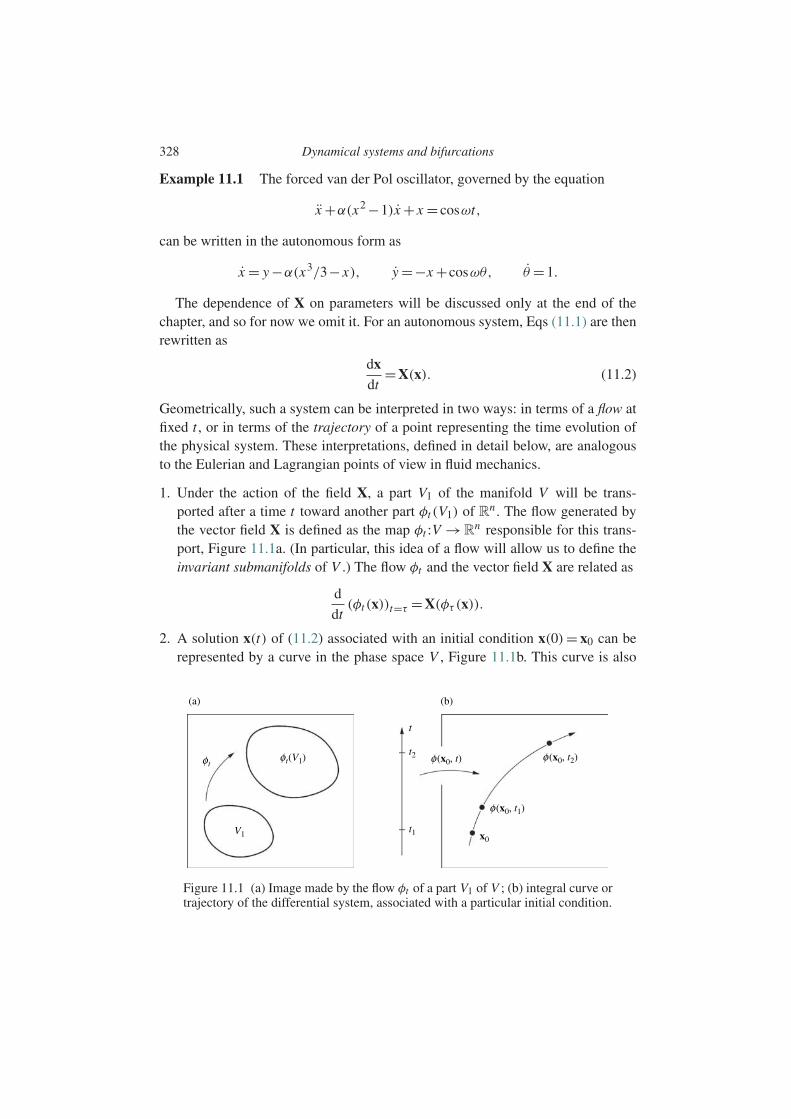
328 Dynamical systems and bifurcations

Example 11.1 The forced van der Pol oscillator, governed by the equation

x +α(x2 −1)x + x = cosωt,

can be written in the autonomous form as

x = y −α(x3/3− x), y =−x +cosωθ, θ =1.

The dependence of X on parameters will be discussed only at the end of thechapter, and so for now we omit it. For an autonomous system, Eqs (11.1) are thenrewritten as

dxdt

=X(x). (11.2)

Geometrically, such a system can be interpreted in two ways: in terms of a flow atfixed t , or in terms of the trajectory of a point representing the time evolution ofthe physical system. These interpretations, defined in detail below, are analogousto the Eulerian and Lagrangian points of view in fluid mechanics.

1. Under the action of the field X, a part V1 of the manifold V will be trans-ported after a time t toward another part φt (V1) of Rn . The flow generated bythe vector field X is defined as the map φt :V →R

n responsible for this trans-port, Figure 11.1a. (In particular, this idea of a flow will allow us to define theinvariant submanifolds of V .) The flow φt and the vector field X are related as

d

dt(φt (x))t=τ =X(φτ (x)).

2. A solution x(t) of (11.2) associated with an initial condition x(0)= x0 can berepresented by a curve in the phase space V , Figure 11.1b. This curve is also

(a)

φtφt(V1)

V1

(b)

φ (x0, t1)

φ (x0, t2)φ (x0, t)

t

t2

t1 x0

Figure 11.1 (a) Image made by the flow φt of a part V1 of V ; (b) integral curve ortrajectory of the differential system, associated with a particular initial condition.

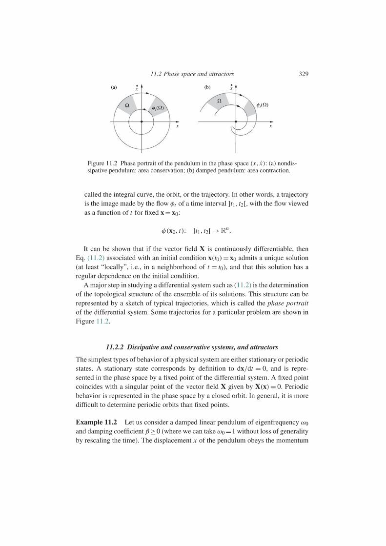
11.2 Phase space and attractors 329

(a) (b)x x

x

ΩΩ

φ t(Ω)φ t(Ω)

x

Figure 11.2 Phase portrait of the pendulum in the phase space (x, x): (a) nondis-sipative pendulum: area conservation; (b) damped pendulum: area contraction.

called the integral curve, the orbit, or the trajectory. In other words, a trajectoryis the image made by the flow φt of a time interval ]t1, t2[, with the flow viewedas a function of t for fixed x=x0:

φ(x0, t): ]t1, t2[→Rn.

It can be shown that if the vector field X is continuously differentiable, thenEq. (11.2) associated with an initial condition x(t0)= x0 admits a unique solution(at least “locally”, i.e., in a neighborhood of t = t0), and that this solution has aregular dependence on the initial condition.

A major step in studying a differential system such as (11.2) is the determinationof the topological structure of the ensemble of its solutions. This structure can berepresented by a sketch of typical trajectories, which is called the phase portraitof the differential system. Some trajectories for a particular problem are shown inFigure 11.2.

11.2.2 Dissipative and conservative systems, and attractors

The simplest types of behavior of a physical system are either stationary or periodicstates. A stationary state corresponds by definition to dx/dt = 0, and is repre-sented in the phase space by a fixed point of the differential system. A fixed pointcoincides with a singular point of the vector field X given by X(x)= 0. Periodicbehavior is represented in the phase space by a closed orbit. In general, it is moredifficult to determine periodic orbits than fixed points.

Example 11.2 Let us consider a damped linear pendulum of eigenfrequency ω0

and damping coefficient β≥0 (where we can take ω0 =1 without loss of generalityby rescaling the time). The displacement x of the pendulum obeys the momentum

330 Dynamical systems and bifurcations

balance (Newton’s second law):

x +β x + x =0.

This second-order differential equation can be written as a system of two first-orderequations:

x = y,

y =−x −βy,

for which the only fixed point in the phase space (x, x) is the origin (0,0). Thetrajectory determined by any initial condition is a spiral converging to this fixedpoint. In the case of a nondissipative pendulum (β=0), the origin is the only fixedpoint as before, and the trajectories are circles centered at the origin. These twocases are shown in Figure 11.2.

Example 11.3 Let us consider a nonlinear oscillator described in polar coordi-nates by the dynamical system

r = r(1−r2),

θ =1.

This system admits a fixed point at the origin r = 0, and a periodic orbit, definedby the circle r = 1 for which r = 0, with period 2π . For r > 1, we get r < 0, whilefor 0 < r < 1, we get r > 0. The origin is therefore an unstable fixed point, andthe periodic orbit is stable. In the phase space, a trajectory coming from any point(except the origin) converges toward the circle r =1.

The essential difference between dissipative and nondissipative (sometimesimproperly called “conservative”) systems amounts to the following property inthe phase space: the flow generated by the vector field of a nondissipative systempreserves volume, while for a dissipative system it contracts or expands an initialvolume. The expansion or contraction is measured by the divergence of the vectorfield. The “compressibility” of dissipative flows is illustrated in Figure 11.2b forthe pendulum discussed above, for which it can be shown that divX=−β.

The fixed points and limit circle discussed in the previous examples representasymptotic behaviors of the system: they are typical examples of attractors of dis-sipative systems. The ensemble of initial conditions from which the system evolvestoward a given attractor is called the basin of attraction of the attractor. In a two-dimensional phase space it can be shown that the only possible attractors are fixedpoints and periodic orbits. In higher dimensions other attractors can exist: tori rep-resenting periodic or quasi-periodic behavior with several frequencies, or “strange

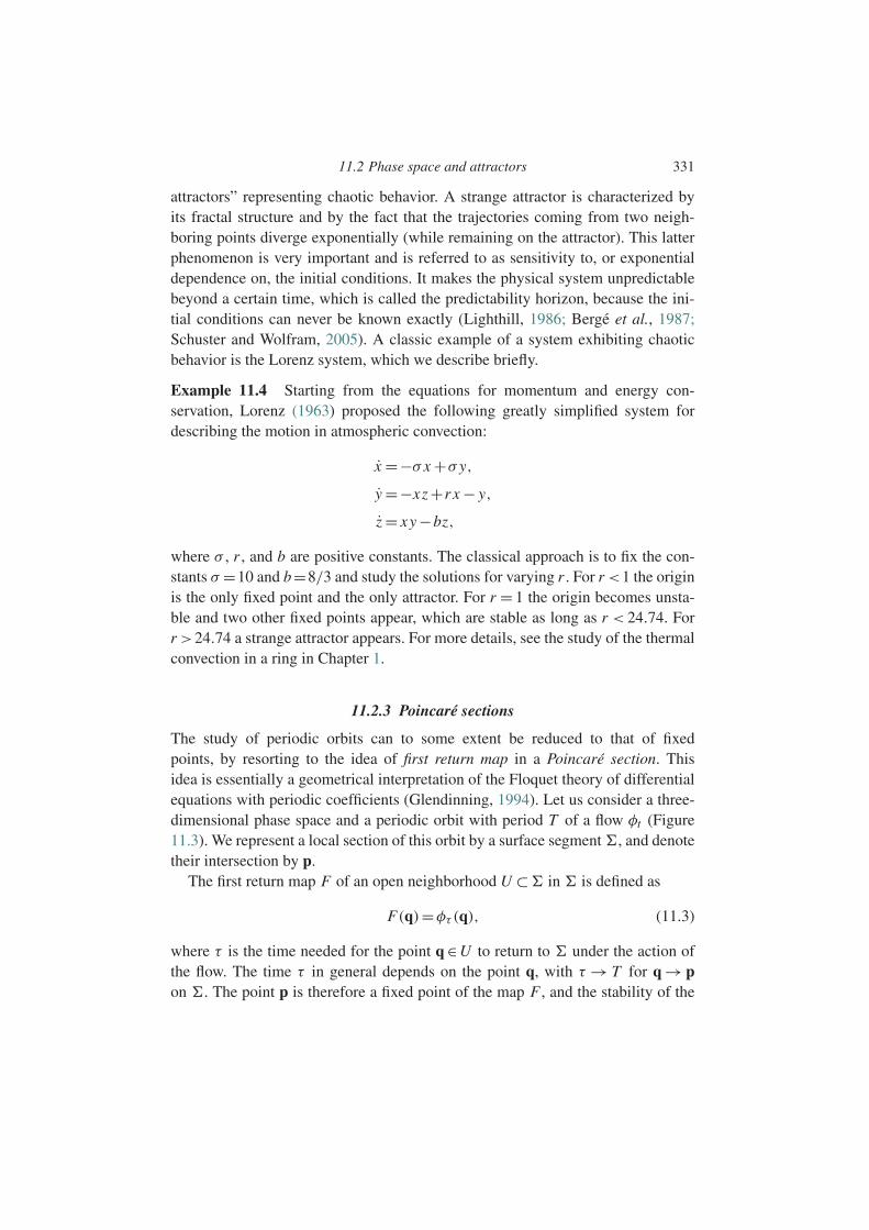
11.2 Phase space and attractors 331

attractors” representing chaotic behavior. A strange attractor is characterized byits fractal structure and by the fact that the trajectories coming from two neigh-boring points diverge exponentially (while remaining on the attractor). This latterphenomenon is very important and is referred to as sensitivity to, or exponentialdependence on, the initial conditions. It makes the physical system unpredictablebeyond a certain time, which is called the predictability horizon, because the ini-tial conditions can never be known exactly (Lighthill, 1986; Berge et al., 1987;Schuster and Wolfram, 2005). A classic example of a system exhibiting chaoticbehavior is the Lorenz system, which we describe briefly.

Example 11.4 Starting from the equations for momentum and energy con-servation, Lorenz (1963) proposed the following greatly simplified system fordescribing the motion in atmospheric convection:

x =−σ x +σ y,

y =−xz +r x − y,

z = xy −bz,

where σ , r , and b are positive constants. The classical approach is to fix the con-stants σ =10 and b=8/3 and study the solutions for varying r . For r <1 the originis the only fixed point and the only attractor. For r = 1 the origin becomes unsta-ble and two other fixed points appear, which are stable as long as r < 24.74. Forr >24.74 a strange attractor appears. For more details, see the study of the thermalconvection in a ring in Chapter 1.

11.2.3 Poincare sections

The study of periodic orbits can to some extent be reduced to that of fixedpoints, by resorting to the idea of first return map in a Poincare section. Thisidea is essentially a geometrical interpretation of the Floquet theory of differentialequations with periodic coefficients (Glendinning, 1994). Let us consider a three-dimensional phase space and a periodic orbit with period T of a flow φt (Figure11.3). We represent a local section of this orbit by a surface segment , and denotetheir intersection by p.

The first return map F of an open neighborhood U ⊂ in is defined as

F(q)=φτ (q), (11.3)

where τ is the time needed for the point q ∈U to return to under the action ofthe flow. The time τ in general depends on the point q, with τ → T for q → pon . The point p is therefore a fixed point of the map F , and the stability of the

332 Dynamical systems and bifurcations

Figure 11.3 Poincare section of a periodic orbit. The intersection point p is afixed point of the first return map F ; the image of a point q on is F(q).

orbit under the action of the flow φt is manifestly related to the stability of thefixed point p for the map F . We note, however, that the definition of the first returnmap involves the flow φt , and therefore the study of the stability of an orbit ingeneral requires that the solutions of the differential system be known! Fortunately,averaging techniques may shortcut the detailed knowledge of these solutions.

The study of first return maps is interesting beyond the subject of Poincaresections. In fact, many physical systems are modeled not by differential equations,but by nonlinear recursion relations, maps, or “discrete dynamical systems” ofthe type

xn+1 =F(xn), (11.4)

where F is a continuously differentiable map. For such discrete systems there is atheory analogous to that of differential systems, but we shall not discuss it here.The logistic map is a simple example of such a recursion relation.

Example 11.5 The logistic map is defined as

xn+1 =λxn(1− xn), x ∈ [0,1], λ>0.

This map possesses a rich variety of surprising phenomena, ranging, for increasingparameter λ, from a simple fixed point F(x)= x for λ<0.75, to periodic dynamicsFm(x)= x (the map F iterated m times), and then to chaotic dynamics for λ>0.89(Feigenbaum, 1978; Tresser and Coullet, 1978). The same sequence of behaviorsis found for all functions F possessing a quadratic extremum, and so the logisticmap is of general interest.

The Henon attractor, which is another classical example of a strange attractor,is studied in Exercise 11.7.1.

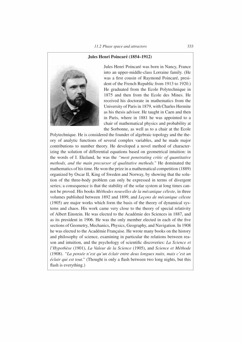
11.2 Phase space and attractors 333

Jules Henri Poincare (1854–1912)

Jules Henri Poincare was born in Nancy, Franceinto an upper-middle-class Lorraine family. (Hewas a first cousin of Raymond Poincare, presi-dent of the French Republic from 1913 to 1920.)He graduated from the Ecole Polytechnique in1875 and then from the Ecole des Mines. Hereceived his doctorate in mathematics from theUniversity of Paris in 1879, with Charles Hermiteas his thesis advisor. He taught in Caen and thenin Paris, where in 1881 he was appointed to achair of mathematical physics and probability atthe Sorbonne, as well as to a chair at the Ecole

Polytechnique. He is considered the founder of algebraic topology and the the-ory of analytic functions of several complex variables, and he made majorcontributions to number theory. He developed a novel method of character-izing the solution of differential equations based on geometrical intuition: inthe words of I. Ekeland, he was the “most penetrating critic of quantitativemethods, and the main precursor of qualitative methods.” He dominated themathematics of his time. He won the prize in a mathematical competition (1889)organized by Oscar II, King of Sweden and Norway, by showing that the solu-tion of the three-body problem can only be expressed in terms of divergentseries; a consequence is that the stability of the solar system at long times can-not be proved. His books Methodes nouvelles de la mecanique celeste, in threevolumes published between 1892 and 1899, and Lecons de mecanique celeste(1905) are major works which form the basis of the theory of dynamical sys-tems and chaos. His work came very close to the theory of special relativityof Albert Einstein. He was elected to the Academie des Sciences in 1887, andas its president in 1906. He was the only member elected in each of the fivesections of Geometry, Mechanics, Physics, Geography, and Navigation. In 1908he was elected to the Academie Francaise. He wrote many books on the historyand philosophy of science, examining in particular the relations between rea-son and intuition, and the psychology of scientific discoveries: La Science etl’Hypothese (1901), La Valeur de la Science (1905), and Science et Methode(1908). “La pensee n’est qu’un eclair entre deux longues nuits, mais c’est uneclair qui est tout.” (Thought is only a flash between two long nights, but thisflash is everything.)

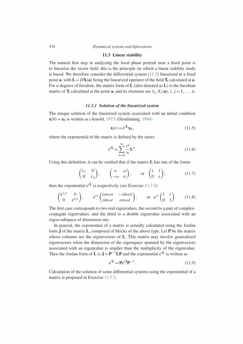
334 Dynamical systems and bifurcations

11.3 Linear stability

The natural first step in analyzing the local phase portrait near a fixed point isto linearize the vector field: this is the principle on which a linear stability studyis based. We therefore consider the differential system (11.2) linearized at a fixedpoint a, with L= DX(a) being the linearized operator of the field X calculated at a.For n degrees of freedom, the matrix form of L (also denoted as L) is the Jacobianmatrix of X calculated at the point a, and its elements are ∂x j Xi (a), i, j =1, . . . ,n.

11.3.1 Solution of the linearized system

The unique solution of the linearized system associated with an initial conditionx(0)=x0 is written as (Arnold, 1973; Glendinning, 1994)

x(t)= etLx0, (11.5)

where the exponential of the matrix is defined by the series

etL =∞∑

n=0

tn

nLn. (11.6)

Using this definition, it can be verified that if the matrix L has one of the forms(λ1 00 λ2

),

(σ ω

−ω σ

), or

(λ 10 λ

), (11.7)

then the exponential etL is respectively (see Exercise 11.7.2)(eλ1t 0

0 eλ2t

), eσ t

(cosωt −sinωtsinωt cosωt

), or eλt

(1 t0 1

). (11.8)

The first case corresponds to two real eigenvalues, the second to a pair of complex-conjugate eigenvalues, and the third to a double eigenvalue associated with aneigen-subspace of dimension one.

In general, the exponential of a matrix is actually calculated using the Jordanform J of the matrix L, composed of blocks of the above type. Let P be the matrixwhose columns are the eigenvectors of L. This matrix may involve generalizedeigenvectors when the dimension of the eigenspace spanned by the eigenvectorsassociated with an eigenvalue is smaller than the multiplicity of the eigenvalue.Then the Jordan form of L is J=P−1LP and the exponential etL is written as

etL =PetJP−1. (11.9)

Calculation of the solution of some differential systems using the exponential of amatrix is proposed in Exercise 11.7.3.

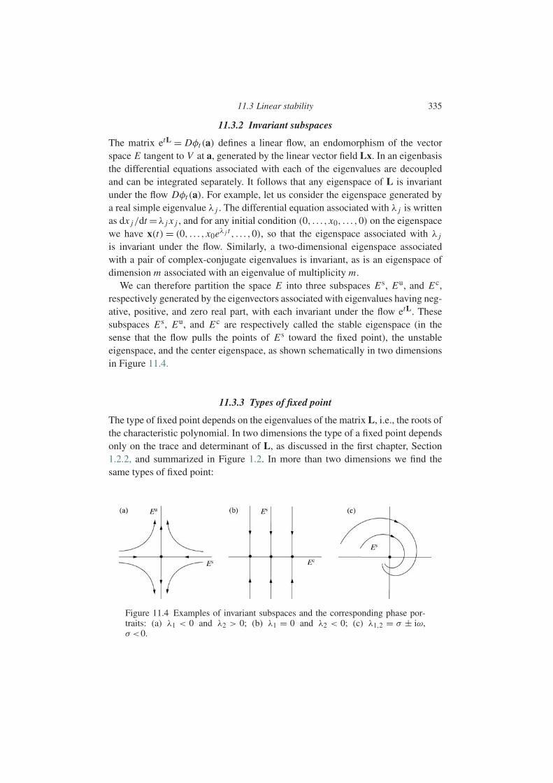
11.3 Linear stability 335

11.3.2 Invariant subspaces

The matrix etL = Dφt (a) defines a linear flow, an endomorphism of the vectorspace E tangent to V at a, generated by the linear vector field Lx. In an eigenbasisthe differential equations associated with each of the eigenvalues are decoupledand can be integrated separately. It follows that any eigenspace of L is invariantunder the flow Dφt (a). For example, let us consider the eigenspace generated bya real simple eigenvalue λ j . The differential equation associated with λ j is writtenas dx j/dt =λ j x j , and for any initial condition (0, . . . , x0, . . . ,0) on the eigenspacewe have x(t) = (0, . . . , x0eλ j t , . . . ,0), so that the eigenspace associated with λ j

is invariant under the flow. Similarly, a two-dimensional eigenspace associatedwith a pair of complex-conjugate eigenvalues is invariant, as is an eigenspace ofdimension m associated with an eigenvalue of multiplicity m.

We can therefore partition the space E into three subspaces E s, Eu, and Ec,respectively generated by the eigenvectors associated with eigenvalues having neg-ative, positive, and zero real part, with each invariant under the flow etL. Thesesubspaces E s, Eu, and Ec are respectively called the stable eigenspace (in thesense that the flow pulls the points of E s toward the fixed point), the unstableeigenspace, and the center eigenspace, as shown schematically in two dimensionsin Figure 11.4.

11.3.3 Types of fixed point

The type of fixed point depends on the eigenvalues of the matrix L, i.e., the roots ofthe characteristic polynomial. In two dimensions the type of a fixed point dependsonly on the trace and determinant of L, as discussed in the first chapter, Section1.2.2, and summarized in Figure 1.2. In more than two dimensions we find thesame types of fixed point:

Figure 11.4 Examples of invariant subspaces and the corresponding phase por-traits: (a) λ1 < 0 and λ2 > 0; (b) λ1 = 0 and λ2 < 0; (c) λ1,2 = σ ± iω,σ <0.

336 Dynamical systems and bifurcations

• When the roots are all real but some positive and others negative, the fixed pointis called a saddle. A saddle is repulsive (unstable), except for the very specialinitial conditions lying on the stable eigenspace.

• When the roots are all real and of the same sign, the fixed point is called a node;it is attractive (stable) if the roots are negative and repulsive (unstable) otherwise.

• When the roots are complex, the fixed point is called a focus, and it is attractive(stable) if the real parts are all negative and repulsive (unstable) otherwise.

• When the roots are purely imaginary the fixed point is a center.

If the real part of each of the eigenvalues is nonzero, the fixed point is termedhyperbolic;1 otherwise the fixed point is termed nonhyperbolic (there exists aneigenvalue whose real part is zero).

11.3.4 “Resemblance” of nonlinear and linearized fields

Once the local phase portrait of the system linearized about a fixed point isobtained, the question arises of how much the linearized system “resembles” theinitial nonlinear system. Intuitively, we can say that two fields resemble each otherif each trajectory of one can be put into correspondence with a trajectory of theother. More precisely, we say that two fields X1 and X2 are orbitally (or topologi-cally) equivalent if there exists a homeomorphism h (if the map h and its inverseexist and are continuous) which transforms each trajectory of X1 into a trajectoryof X2 while conserving the direction of the motion. It can then be shown that afield X which is continuously differentiable on a manifold V and its version L,linearized at a fixed point a, are topologically equivalent if all the eigenvalues of Lhave nonzero real part, i.e., if the fixed point is hyperbolic (the Hartman–Grobmantheorem).

An important consequence of the Hartman–Grobman theorem is that if the fixedpoint a is hyperbolic, the linearization procedure can be used to find the topologicaltype of the fixed point (node, focus, saddle, etc.) and to sketch the shape of thephase portrait in its vicinity. If a is not hyperbolic, the linearization does not giveany information about the stability of the fixed point, which is determined by termsof higher degree. Only by taking into account these higher-degree terms in X is itpossible to get an idea of the phase portrait, which will take us back to the subjectof nonlinear stability.

Example 11.6 Let us consider the vector field given by

X(x, y)= [y + xφ(x2 + y2),−x + yφ(x2 + y2)], (11.10)

1 Note that for nondissipative (conservative) systems, fixed points are either saddles or centers, so that hyperbolicpoints and saddles are the same, and centers are also called elliptic points.

11.3 Linear stability 337

where φ is a function such that φ(0)=0. The linearized field is L(x, y)= (y,−x),and it possesses two purely imaginary eigenvalues. The fixed point is therefore nothyperbolic, and the trajectories of L are circles centered at the origin. The phaseportrait of X, on the other hand, actually depends on the choice of the functionφ. Let us change to polar coordinates (r,θ). The trajectories are then defined bythe equation dr/dθ = rφ(r2). For any value of r which makes φ vanish, the circleof radius r is a trajectory of X. If, for example, the function φ vanishes for thetwo values a and b of the radius r and is positive between a and b, then anytrajectory starting from a point of the ring located between r = a and r = b willtend towards the outer circle of radius b. There are therefore at least as manynonorbitally equivalent phase portraits as there are ways of choosing the zeros ofthe function φ!

We note that the resemblance defined above involves only the topological prop-erties of the trajectories and not the law of motion (for example, the period of aclosed orbit). It is possible to define a stronger resemblance between the field Xand its linearized version L which preserves the law of motion along the trajecto-ries; this requires that the transport homeomorphism h be differentiable (i.e., thatit be a diffeomorphism). The resemblance will be the stronger the higher the dif-ferentiability class of h. However, this differentiability gives rise to nonresonanceconditions between the eigenvalues of L (the Sternberg theorem).

Example 11.7 Let us consider the vector field given by

X(x, y)= (2x + y2, y). (11.11)

The field linearized at the origin is L(x, y)= (2x, y), and the flows generated by Land X are respectively

φLt (x, y)= (xe2t , yet ), φX

t (x, y)= [(x + t y2)e2t , yet ]. (11.12)

These flows look similar and it can be shown that they are topologically equivalent,but the map which permits the trajectories of one to be transformed into those ofthe other is of class C1 at most. Indeed, let us try to construct two functions f (x, y)and g(x, y) with nonzero Jacobian at the origin and with

φLt [ f (x, y),g(x, y)]= [ f (φX

t (x, y),g(φXt (x, y))]. (11.13)

For our particular case this gives

e2t f (x, y)= f [(x + t y2)e2t , yet ]. (11.14)

However, it can be verified by differentiating twice with respect to y that as soonas f is of class C2, this latter relation, even for a single nonzero value of t , impliesthat the two partial derivatives of f at 0 are zero.

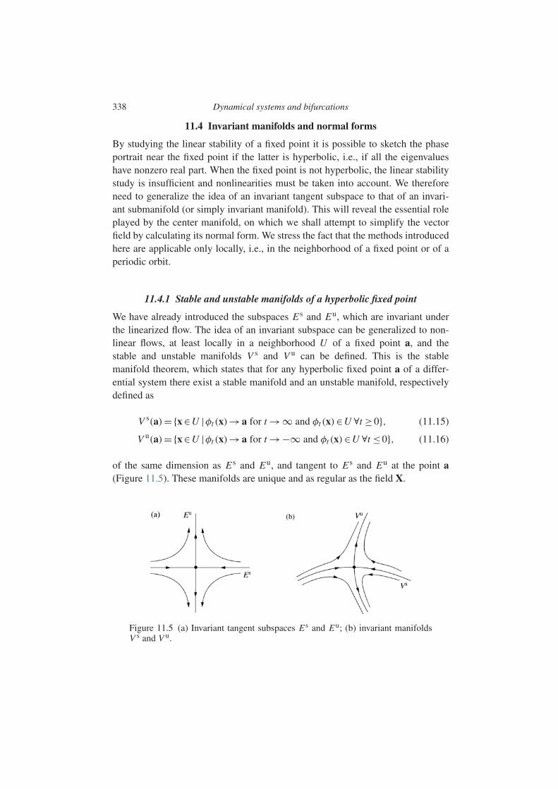
338 Dynamical systems and bifurcations

11.4 Invariant manifolds and normal forms

By studying the linear stability of a fixed point it is possible to sketch the phaseportrait near the fixed point if the latter is hyperbolic, i.e., if all the eigenvalueshave nonzero real part. When the fixed point is not hyperbolic, the linear stabilitystudy is insufficient and nonlinearities must be taken into account. We thereforeneed to generalize the idea of an invariant tangent subspace to that of an invari-ant submanifold (or simply invariant manifold). This will reveal the essential roleplayed by the center manifold, on which we shall attempt to simplify the vectorfield by calculating its normal form. We stress the fact that the methods introducedhere are applicable only locally, i.e., in the neighborhood of a fixed point or of aperiodic orbit.

11.4.1 Stable and unstable manifolds of a hyperbolic fixed point

We have already introduced the subspaces E s and Eu, which are invariant underthe linearized flow. The idea of an invariant subspace can be generalized to non-linear flows, at least locally in a neighborhood U of a fixed point a, and thestable and unstable manifolds V s and V u can be defined. This is the stablemanifold theorem, which states that for any hyperbolic fixed point a of a differ-ential system there exist a stable manifold and an unstable manifold, respectivelydefined as

V s(a)=x∈U |φt (x)→a for t →∞ and φt (x)∈U ∀t ≥0, (11.15)

V u(a)=x∈U |φt (x)→a for t →−∞ and φt (x)∈U ∀t ≤0, (11.16)

of the same dimension as E s and Eu, and tangent to E s and Eu at the point a(Figure 11.5). These manifolds are unique and as regular as the field X.

(b)

Figure 11.5 (a) Invariant tangent subspaces E s and Eu; (b) invariant manifoldsV s and V u.

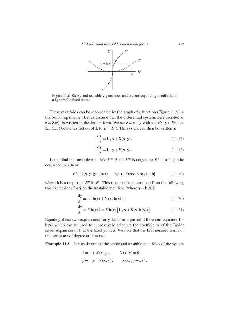
11.4 Invariant manifolds and normal forms 339

Figure 11.6 Stable and unstable eigenspaces and the corresponding manifolds ofa hyperbolic fixed point.

These manifolds can be represented by the graph of a function (Figure 11.6) inthe following manner. Let us assume that the differential system, here denoted asz = Z(z), is written in the Jordan form. We set z = x+y with x ∈ Eu, y ∈ E s. LetL+ (L−) be the restriction of L to Eu (E s). The system can then be written as

dxdt

=L+x+X(x,y), (11.17)

dydt

=L−y+Y(x,y). (11.18)

Let us find the unstable manifold V u. Since V u is tangent to Eu at a, it can bedescribed locally as

V u =(x,y)|y=h(x), h(a)=0 and Dh(a)=0, (11.19)

where h is a map from Eu in E s. This map can be determined from the followingtwo expressions for y on the unstable manifold [where y=h(x)]:

dydt

=L−h(x)+Y (x,h(x)) , (11.20)

dydt

= Dh(x)x = Dh(x)[L+x+X(x,h(x))

]. (11.21)

Equating these two expressions for y leads to a partial differential equation forh(x) which can be used to successively calculate the coefficients of the Taylorseries expansion of h at the fixed point a. We note that the first nonzero terms ofthis series are of degree at least two.

Example 11.8 Let us determine the stable and unstable manifolds of the system

x = x + X (x, y), X (x, y)=0,

y =−y +Y (x, y), Y (x, y)=ax2.

340 Dynamical systems and bifurcations

The only fixed point of this system is the origin, the eigenvalues of the linearizedsystem are 1 and −1, and the associated eigenspaces are respectively the x-axisand the y-axis. We seek the unstable manifold in the form y = h(x). Setting thetwo expressions for y on the unstable manifold,

y =−y +Y (x,h(x)),

y =h′(x)x =h′(x) [x + X (x,h(x))] ,

equal to each other, and seeking h(x) in the form of a polynomial series h(x)=∑i hi xi , we obtain

−∑

i

hi xi +ax2 =

∑i

ihi xi ,

from which we find h2 = a/3 and hi = 0 for i ≥ 3. The unstable manifold is thendefined by y(x)=ax3/3.

Some other calculations of stable and unstable manifolds are proposed inExercises 11.7.4 and 11.7.5.

11.4.2 The center manifold

In the case of a nonhyperbolic fixed point a it is tempting to generalize the pre-ceding definitions and introduce, in addition to the stable and unstable manifolds,the center manifold tangent to the center subspace at the point a. It can be provedthat such a center manifold V c exists and has the same dimension as Ec: this is thecenter manifold theorem. However, two technical difficulties arise which were notpresent in the stable manifold theorem: (i) V c is not necessarily unique, and (ii) if Xbelongs to the class C r, then V c belongs only to the class C r−1 (see Guckenheimerand Holmes, 1983, p. 124). However, these two details are unimportant for ourpurposes.

The determination of the center manifold via a function y=h(x) is done exactlyas for the stable and unstable manifolds. In the important case of marginal stability,where all the eigenvalues have negative real part except a few whose real part iszero, it is sufficient to rewrite Eqs (11.17)–(11.21) replacing L+, V u, and Eu byL0, V c, and Ec. The function h(x) is then the solution of the partial differentialequation

L−h(x)+Y (x,h(x))= Dh(x) [L0x+X(x,h(x))] , (11.22)

which can be solved by seeking h(x) in the form of a Taylor series.

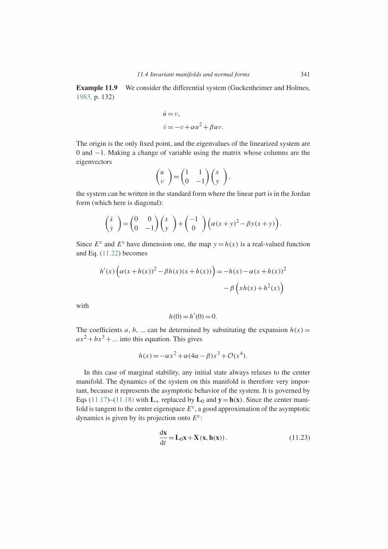
11.4 Invariant manifolds and normal forms 341

Example 11.9 We consider the differential system (Guckenheimer and Holmes,1983, p. 132)

u = v,

v=−v+αu2 +βuv.

The origin is the only fixed point, and the eigenvalues of the linearized system are0 and −1. Making a change of variable using the matrix whose columns are theeigenvectors (

uv

)=(

1 10 −1

)(xy

),

the system can be written in the standard form where the linear part is in the Jordanform (which here is diagonal):(

xy

)=(

0 00 −1

)(xy

)+(−1

0

)(α(x + y)2 −βy(x + y)

).

Since Ec and E s have dimension one, the map y = h(x) is a real-valued functionand Eq. (11.22) becomes

h′(x)(α(x +h(x))2 −βh(x)(x +h(x))

)=−h(x)−α(x +h(x))2

−β(

xh(x)+h2(x))

with

h(0)=h′(0)=0.

The coefficients a, b, ... can be determined by substituting the expansion h(x)=ax2 +bx3 + ... into this equation. This gives

h(x)=−αx2 +α(4α−β)x3 +O(x4).

In this case of marginal stability, any initial state always relaxes to the centermanifold. The dynamics of the system on this manifold is therefore very impor-tant, because it represents the asymptotic behavior of the system. It is governed byEqs (11.17)–(11.18) with L+ replaced by L0 and y=h(x). Since the center mani-fold is tangent to the center eigenspace Ec, a good approximation of the asymptoticdynamics is given by its projection onto Ec:

dxdt

=L0x+X (x,h(x)) . (11.23)

342 Dynamical systems and bifurcations

Example 11.10 Continuing with the above example, a good approximation ofthe dynamics on the center manifold is

x =αx2 +α(β−2α)x3 +O(x4).

We note that at second order we can obtain the same result without calculating thecenter manifold, by inserting into Eq. (11.23) the approximation h(x)=0+O(x2),which is called the tangent space approximation.

In Exercise 11.7.6 we propose the calculation of a center manifold.

11.4.3 The normal form of a vector field

Calculating the normal form of a vector field involves finding a coordinate trans-formation that simplifies the expression for this vector field as much as possible.To motivate the existence of such a transformation, let us consider a linear vectorfield. It can easily be imagined that a nonlinear transformation can transform thislinear field into a nonlinear field. The nonlinearities that arise in this case are onlycomplications due to the use of a coordinate system poorly adapted to the problem.Conversely, one can ask if, for a given nonlinear field, some of the nonlinearities –perhaps all of them – might not be due to the use of a less than optimal choice ofcoordinate system.

We are going to show that in fact it is possible to find a “natural” curvilinearcoordinate system in which the dynamical system is simpler to study. This is thenormal form theorem. Moreover, such a coordinate system may reveal propertiesof the system, in particular, symmetry properties, that were hidden in the originalformulation. However, it appears that some nonlinearities are resistant to any coor-dinate transformation and cannot be eliminated. Such irreducible nonlinearities aretermed resonant and are important from the viewpoint of the system dynamics. Forexample, the differential system

x =2x + y2, y = y (11.24)

cannot be written as

u =2u, v= v (11.25)

in any local coordinate system (u,v), because the nonlinearity y2 is resonant.Let us therefore consider a differential system defined by a regular vector field

on a manifold V of dimension n. The origin is assumed to be a fixed point nearwhich the field can be expanded in a Taylor series:

dxdt

=X(x)=Lx+X2(x)+ ...+XN (x)+O(|x|N+1). (11.26)

11.4 Invariant manifolds and normal forms 343

Here L = DX(0) is the Jacobian operator of X, assumed to be diagonal, and Xr

is the vector function whose components Xri , i = 1, . . . ,n, contain the terms ofdegree r ≥2. Defining

Mr =m= (m1,m2, . . . ,mn)∈Nn with

∑m j = r,

Xr (x) can be written as

Xr (x)=∑

m∈Mr

Xmxm with xm = xm11 xm2

2 ...xmnn , (11.27)

where the Xm are vectors whose n components represent the coefficients ofmonomials of degree r . For example, in two dimensions, M1 = (1,0), (1,0),M2 =(2,0), (1,1), (0,2), and X2 is written as

X2 =X(2,0)x2 +X(1,1)xy +X(0,2)y

2. (11.28)

The calculation of the normal form of the field X(x) consists of construct-ing a sequence of coordinate transformations preserving the linear part L of thefield (called “near-identity” transformations) which allow the elimination of asmany nonlinear terms of higher and higher order as possible. Let us consider adifferential system of the form

dxdt

=Lx+Xr (x)+O(|x|r+1), r ≥2, (11.29)

and seek a coordinate transformation of the form

y=x+φr (x), r ≥2, (11.30)

where φr contains only terms of degree r , which allows the system (11.29) to beexpressed in the new coordinates as

dydt

=Ly+O(|y|r+1), r ≥2. (11.31)

If this transformation exists, it is therefore possible by repeating the operation tosuccessively eliminate all the nonlinear terms.

Let us show the reasoning for the components of the differential system. Thei th component of the transformation (11.30) is

yi = xi +∑

m∈Mr

φm,i xm, (11.32)

the inverse of which is written as

xi = yi −∑

m∈Mr

φm,i ym +O(|y|r+1) (11.33)

344 Dynamical systems and bifurcations

(the correctness of this inversion can be found by using an example in one dimen-sion and a polynomial of second degree: y = x +ax2). The system can be writtenin the form (11.31) by first differentiating (11.32) with respect to the time:

yi = xi +∑

m∈Mr

φm,idxm

dt. (11.34)

Successively using (11.29) and then (11.33) with xm = ym +O(|y|r+1), xi can bewritten as

xi =λi xi +∑

m∈Mr

Xm,i xm

=λi yi −λi

∑m∈Mr

φm,i ym +∑

m∈Mr

Xm,i ym +O(|y|r+1). (11.35)

On the other hand, defining (m,λ) =∑k=1,n mkλk , the derivative of xm can bewritten as

dxm

dt=∑

k=1,n

xk

xkmkxm

= (m,λ)xm +O(|x|r+1)

= (m,λ)ym +O(|y|r+1). (11.36)

Substituting (11.35) and (11.36) into (11.34), we obtain an approximation of thedynamical system in the transformed coordinates:

yi =λi yi +∑

m∈Mr

(Xm,i − [λi −(m,λ)]φm,i

)ym +O(|y|r+1). (11.37)

We therefore see that if for all m∈ Mr the conditions

λi −(m,λ) =0 (11.38)

are satisfied, then it is possible to choose the φm,i so as to cancel the terms oforder r . These conditions are called the nonresonance conditions at order r of theeigenvalues. The desired coordinate transformation is then written explicitly as

φm,i = Xm,i

λi −(m,λ). (11.39)

If for a particular m ∈ Mr the nonresonance condition is not satisfied, the corre-sponding monomial is termed resonant and cannot be eliminated. We note that

11.5 Structural stability and genericity 345

whether or not a nonlinear term is resonant depends only on the eigenvalues andtherefore on the linear terms. Let us make a few observations:

1. The right-hand side of Eq. (11.37) contains, aside from the linear term λi yi ,only terms of degree r or higher. In particular, if X2, . . . ,Xr−1 are zero beforethe transformation, they are always zero after it.

2. It can be verified that the resonant terms appearing at order r are not modifiedby later transformations to eliminate the terms of order higher than r . On thecontrary, the nonlinearities of order higher than r are in general modified.

3. The preceding discussion rests on the hypothesis that the fixed point is hyper-bolic and that L is diagonal. The arguments can be generalized to the nonhy-perbolic case and nondiagonal L; see Guckenheimer and Holmes (1983, §3.3)and Elphick et al. (1987) for a more formal and general presentation.

Therefore, we now possess two fundamental tools for studying a system ofdifferential equations:

• The center manifold theorem, which allows us to focus on the asymptotic behav-ior of the system on the center manifold of low dimension (in practice, projectionof the dynamics on the center subspace is usually sufficient).

• The normal-form theorem, which allows the differential system to be expressedmore simply on the center manifold by the introduction of a suitable coordinatesystem.

Exercises 11.7.7 and 11.7.8 propose resonance and normal-form calculations.

11.5 Structural stability and genericity

11.5.1 The basic problem

The question we tackle here which will lead us to the study of bifurcations is: fora given system, what happens as one of the system parameters varies? Does thephase portrait remain qualitatively the same, or does it undergo profound changessuch as modification of the type or even disappearance of a fixed point?

Another essential question from the physical point of view is the following:is the system of equations sufficiently “robust” to not only describe the observedphenomena but also to make reliable predictions? Would some physical effect,neglected in the modeling and whose inclusion would lead to a system of “simi-lar” equations, completely change the nature of the solutions? In other words, isthe system of equations both sufficiently general and its predictions sufficiently“robust” to small changes to it? What happens if it is “perturbed” by the additionof a small term?

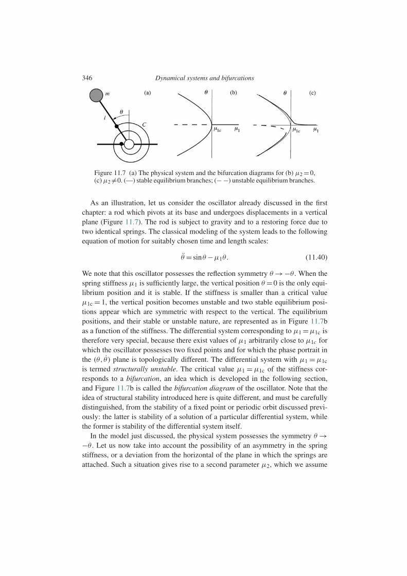
346 Dynamical systems and bifurcations

Figure 11.7 (a) The physical system and the bifurcation diagrams for (b) µ2 =0,(c) µ2 =0. (—) stable equilibrium branches; (− −) unstable equilibrium branches.

As an illustration, let us consider the oscillator already discussed in the firstchapter: a rod which pivots at its base and undergoes displacements in a verticalplane (Figure 11.7). The rod is subject to gravity and to a restoring force due totwo identical springs. The classical modeling of the system leads to the followingequation of motion for suitably chosen time and length scales:

θ = sinθ −µ1θ. (11.40)

We note that this oscillator possesses the reflection symmetry θ →−θ . When thespring stiffness µ1 is sufficiently large, the vertical position θ =0 is the only equi-librium position and it is stable. If the stiffness is smaller than a critical valueµ1c = 1, the vertical position becomes unstable and two stable equilibrium posi-tions appear which are symmetric with respect to the vertical. The equilibriumpositions, and their stable or unstable nature, are represented as in Figure 11.7bas a function of the stiffness. The differential system corresponding to µ1 =µ1c istherefore very special, because there exist values of µ1 arbitrarily close to µ1c forwhich the oscillator possesses two fixed points and for which the phase portrait inthe (θ, θ ) plane is topologically different. The differential system with µ1 =µ1c

is termed structurally unstable. The critical value µ1 = µ1c of the stiffness cor-responds to a bifurcation, an idea which is developed in the following section,and Figure 11.7b is called the bifurcation diagram of the oscillator. Note that theidea of structural stability introduced here is quite different, and must be carefullydistinguished, from the stability of a fixed point or periodic orbit discussed previ-ously: the latter is stability of a solution of a particular differential system, whilethe former is stability of the differential system itself.

In the model just discussed, the physical system possesses the symmetry θ →−θ . Let us now take into account the possibility of an asymmetry in the springstiffness, or a deviation from the horizontal of the plane in which the springs areattached. Such a situation gives rise to a second parameter µ2, which we assume

11.5 Structural stability and genericity 347

to be small. The modeling equation becomes

θ = sinθ −µ1θ +µ2. (11.41)

The symmetry θ →−θ is now broken. It can be checked that the bifurcation dia-gram is that represented in Figure 11.7c, which is qualitatively different fromthat of Figure 11.7b. For example, for µ1 slightly less than µ1c there is only asingle equilibrium position. In the parameter plane (µ1,µ2) the locus of pointscorresponding to the bifurcation can be represented by a curve. The model includ-ing µ2 now correctly represents the physical system no matter what its “hidden”imperfections are, and so this model is said to be generic.

As a second example, let us consider the Descartes laws of reflection of a lightray on a planar mirror. These laws are found to be consistent with experiment –away from the critical angle – in spite of the inevitable defects in the planarity ofthe mirror and in the homogeneity of its reflection properties. Here, the assumptionthat the mirror is perfectly planar is fine, in contrast to the symmetry hypothesisof the preceding example. Small imperfections of the mirror can be neglected: theDescartes laws can also be said to be generic.

11.5.2 Definitions

Let us recall the two questions posed in the introduction to this section:

• Does a vector field subject to small perturbations, induced for example by thevariation of a parameter, resemble the initial field (structural stability)?

• Is a field chosen at random representative of the ensemble of fields to which itbelongs (genericity)?

Now we need to make the ideas of structural stability and genericity more pre-cise. These ideas are in fact related to an old problem in geometry, that of the“general position,” which is formalized by introducing the mathematical conceptsof an open set and a dense set. Let us explain this by means of a simple example.

We consider the set of triplets of lines in a plane, supplied with a suitable topol-ogy allowing the “distance between two triplets” to be defined precisely. On theone hand, any deformation of a triangle, provided it is small, remains a triangle:the set of triplets forming a triangle is open in the set of triplets of lines in theplane. On the other hand, a triplet of lines “almost always” forms a triangle. Here“almost always” means that triplets not forming a triangle are rare, and that therealways exists an arbitrarily small deformation which transforms such a triplet intoa triplet forming a triangle. The set of triplets forming a triangle is said to be densewithin the set of triplets of lines in the plane.

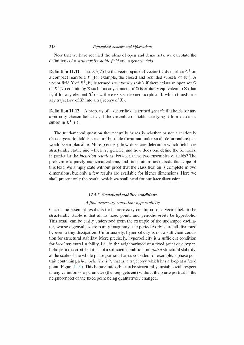
348 Dynamical systems and bifurcations

Now that we have recalled the ideas of open and dense sets, we can state thedefinitions of a structurally stable field and a generic field.

Definition 11.11 Let E1(V ) be the vector space of vector fields of class C1 ona compact manifold V (for example, the closed and bounded subsets of Rn). Avector field X of E1(V ) is termed structurally stable if there exists an open set of E1(V ) containing X such that any element of is orbitally equivalent to X (thatis, if for any element X′ of there exists a homeomorphism h which transformsany trajectory of X′ into a trajectory of X).

Definition 11.12 A property of a vector field is termed generic if it holds for anyarbitrarily chosen field, i.e., if the ensemble of fields satisfying it forms a densesubset in E1(V ).

The fundamental question that naturally arises is whether or not a randomlychosen generic field is structurally stable (invariant under small deformations), aswould seem plausible. More precisely, how does one determine which fields arestructurally stable and which are generic, and how does one define the relations,in particular the inclusion relations, between these two ensembles of fields? Theproblem is a purely mathematical one, and its solution lies outside the scope ofthis text. We simply state without proof that the classification is complete in twodimensions, but only a few results are available for higher dimensions. Here weshall present only the results which we shall need for our later discussion.

11.5.3 Structural stability conditions

A first necessary condition: hyperbolicity

One of the essential results is that a necessary condition for a vector field to bestructurally stable is that all its fixed points and periodic orbits be hyperbolic.This result can be easily understood from the example of the undamped oscilla-tor, whose eigenvalues are purely imaginary: the periodic orbits are all disruptedby even a tiny dissipation. Unfortunately, hyperbolicity is not a sufficient condi-tion for structural stability. More precisely, hyperbolicity is a sufficient conditionfor local structural stability, i.e., in the neighborhood of a fixed point or a hyper-bolic periodic orbit, but it is not a sufficient condition for global structural stability,at the scale of the whole phase portrait. Let us consider, for example, a phase por-trait containing a homoclinic orbit, that is, a trajectory which has a loop at a fixedpoint (Figure 11.9). This homoclinic orbit can be structurally unstable with respectto any variation of a parameter (the loop gets cut) without the phase portrait in theneighborhood of the fixed point being qualitatively changed.

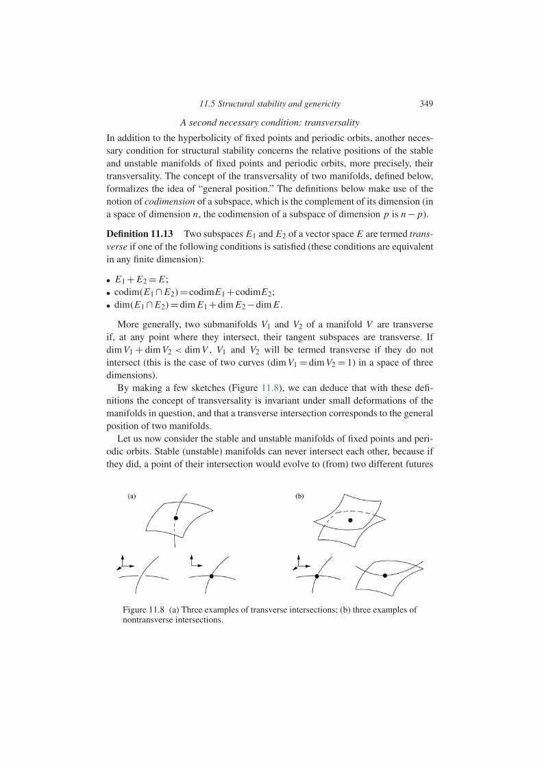
11.5 Structural stability and genericity 349

A second necessary condition: transversality

In addition to the hyperbolicity of fixed points and periodic orbits, another neces-sary condition for structural stability concerns the relative positions of the stableand unstable manifolds of fixed points and periodic orbits, more precisely, theirtransversality. The concept of the transversality of two manifolds, defined below,formalizes the idea of “general position.” The definitions below make use of thenotion of codimension of a subspace, which is the complement of its dimension (ina space of dimension n, the codimension of a subspace of dimension p is n − p).

Definition 11.13 Two subspaces E1 and E2 of a vector space E are termed trans-verse if one of the following conditions is satisfied (these conditions are equivalentin any finite dimension):

• E1 + E2 = E ;• codim(E1 ∩ E2)= codimE1 +codimE2;• dim(E1 ∩ E2)=dim E1 +dim E2 −dim E .

More generally, two submanifolds V1 and V2 of a manifold V are transverseif, at any point where they intersect, their tangent subspaces are transverse. Ifdim V1 + dim V2 < dim V , V1 and V2 will be termed transverse if they do notintersect (this is the case of two curves (dim V1 = dim V2 = 1) in a space of threedimensions).

By making a few sketches (Figure 11.8), we can deduce that with these defi-nitions the concept of transversality is invariant under small deformations of themanifolds in question, and that a transverse intersection corresponds to the generalposition of two manifolds.

Let us now consider the stable and unstable manifolds of fixed points and peri-odic orbits. Stable (unstable) manifolds can never intersect each other, because ifthey did, a point of their intersection would evolve to (from) two different futures

Figure 11.8 (a) Three examples of transverse intersections; (b) three examples ofnontransverse intersections.

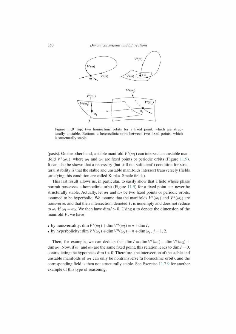
350 Dynamical systems and bifurcations

Figure 11.9 Top: two homoclinic orbits for a fixed point, which are struc-turally unstable. Bottom: a heteroclinic orbit between two fixed points, whichis structurally stable.

(pasts). On the other hand, a stable manifold V s(ω1) can intersect an unstable man-ifold V u(ω2), where ω1 and ω2 are fixed points or periodic orbits (Figure 11.9).It can also be shown that a necessary (but still not sufficient!) condition for struc-tural stability is that the stable and unstable manifolds intersect transversely (fieldssatisfying this condition are called Kupka–Smale fields).

This last result allows us, in particular, to easily show that a field whose phaseportrait possesses a homoclinic orbit (Figure 11.9) for a fixed point can never bestructurally stable. Actually, let ω1 and ω2 be two fixed points or periodic orbits,assumed to be hyperbolic. We assume that the manifolds V s(ω1) and V u(ω2) aretransverse, and that their intersection, denoted I , is nonempty and does not reduceto ω1 if ω1 =ω2. We then have dimI > 0. Using n to denote the dimension of themanifold V , we have

• by transversality: dim V s(ω1)+dim V u(ω2)=n +dim I ,• by hyperbolicity: dim V s(ω j )+dim V u(ω j )=n +dimω j , j =1,2.

Then, for example, we can deduce that dim I = dim V s(ω1)− dim V s(ω2)+dimω2. Now, if ω1 and ω2 are the same fixed point, this relation leads to dim I =0,contradicting the hypothesis dim I >0. Therefore, the intersection of the stable andunstable manifolds of ω1 can only be nontransverse (a homoclinic orbit), and thecorresponding field is then not structurally stable. See Exercise 11.7.9 for anotherexample of this type of reasoning.

11.6 Bifurcations 351

Necessary and sufficient conditions

By imposing additional restrictions on the vector fields it is possible to obtainclasses of structurally stable fields. Particular examples are gradient fields (such asX(x)=∇U (x)) and Morse–Smale fields (Guckenheimer and Holmes, 1983, §1.7).

In two dimensions the situation is easier and it can be shown (the Peixototheorem) that in a planar phase space, the Kupka–Smale fields (which satisfyhyperbolicity and transversality of the stable and unstable manifolds) are struc-turally stable and generic (the Peixoto theorem is in fact a bit more general, andapplies to the case of nonplanar phase spaces such as tori).

11.6 Bifurcations

11.6.1 Introduction

The behavior of any physical system generally depends on a number of parame-ters. The response of the system to variations in these parameters is usually regular,but there may exist particular parameter values for which the system suddenlyadopts a qualitatively different behavior. Such a change of behavior is called abifurcation. In the example of the pendulum discussed in the preceding section,the passage from one to two equilibrium positions was a bifurcation. The hydrody-namical instabilities discussed in previous chapters also correspond to bifurcations.For example, the transition between the conductive and convective regimes in theRayleigh–Benard problem is a bifurcation governed by the Rayleigh number.

A continuous increase of a parameter generally leads to a cascade of suchtransitions, with the observed behavior becoming more and more complex or dis-ordered. For many physical systems an initial stable stationary state is followedby periodic behavior, which becomes unstable in turn, giving rise to phenomenasuch as period-doubling, intermittency, quasi-periodicity, and perhaps ultimatelyunpredictable, chaotic behavior. The fact that the same cascade of transitions orbifurcations occurs for mechanical, electrical, and chemical systems suggests thatthese bifurcations are universal in a certain sense, which has greatly stimulatedtheir study.

11.6.2 Definition of a bifurcation

How can a bifurcation be defined precisely? Let us consider a differential systemon a manifold V , depending on a parameter µ (µ∈R

m if there are m parameters):

dxdt

=X(x,µ). (11.42)

352 Dynamical systems and bifurcations

A natural definition of a bifurcation might be the following. We can say that thevector field X(x,µ) undergoes a bifurcation for the value µ=µc of the parameterif, at this value, the field is not structurally stable. This definition corresponds wellto the intuitive idea of a bifurcation: on either side of µc the solutions are qualita-tively different, corresponding to qualitatively different behaviors of the physicalsystem. However, some peculiarities with this definition may arise in dimensionshigher than two, where, as already noted, structurally stable fields do not form adense set. It is therefore possible to find generic families of vector fields in whichno element is structurally stable: for such a family, all the parameter values will bebifurcation values! To avoid this inconvenience and to ensure that the bifurcationvalues are isolated, we restrict the preceding definition as follows:

Definition 11.14 The family X(x,µ) of vector fields is said to present a bifur-cation for the parameter value µc if the field X(x,µc) is not of the Kupka–Smaletype, that is,

• if one of the fixed points or one of the periodic orbits loses its hyperbolicity (alocal accident which leads to the definition of a local bifurcation); or

• if one stable manifold and one unstable manifold no longer intersect transversely(an accident which globally affects the phase portrait, corresponding to a globalbifurcation).

11.6.3 Codimension of a bifurcation

In general, a model – in this context a system of ordinary differential equations –involves several parameters. A bifurcation condition then amounts to a relationbetween these various parameters:

f (µ1, . . . ,µm)=0. (11.43)

Geometrically, this relation defines a hypersurface in the parameter space Rm

of dimension m −1: thus can be said to have codimension one. Therefore, inmoving along a curve of Rm of dimension one, in general one will intersect thehypersurface (Figure 11.10). At the cost of changing the reference frame, it issufficient to vary a single parameter to reach the bifurcation. Such a bifurcationwill be referred to as a bifurcation of codimension one.

If the bifurcation condition involves two relations of the type (11.43), thebifurcation points will be located on the intersection of the two correspondinghypersurfaces 1 and 2. To reach this intersection of dimension m −2, or codi-mension 2, the two parameters must be varied independently. Such a bifurcationwill be referred to as a bifurcation of codimension two. Bifurcations of highercodimension are defined analogously.

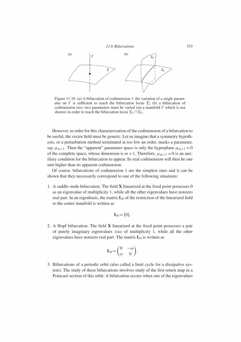
11.6 Bifurcations 353

Σ

Γ Σ2

Σ1

(a) (b)

Figure 11.10 (a) A bifurcation of codimension 1: the variation of a single param-eter on is sufficient to reach the bifurcation locus ; (b) a bifurcation ofcodimension two: two parameters must be varied (on a manifold which is notshown) in order to reach the bifurcation locus 1 ∩2.

However, in order for this characterization of the codimension of a bifurcation tobe useful, the vector field must be generic. Let us imagine that a symmetry hypoth-esis, or a perturbation method terminated at too low an order, masks a parameter,say µm+1. Then the “apparent” parameter space is only the hyperplane µm+1 = 0of the complete space, whose dimension is m +1. Therefore, µm+1 = 0 is an aux-iliary condition for the bifurcation to appear. Its real codimension will then be oneunit higher than its apparent codimension.

Of course, bifurcations of codimension 1 are the simplest ones and it can beshown that they necessarily correspond to one of the following situations:

1. A saddle–node bifurcation. The field X linearized at the fixed point possesses 0as an eigenvalue of multiplicity 1, while all the other eigenvalues have nonzeroreal part. In an eigenbasis, the matrix L0 of the restriction of the linearized fieldto the center manifold is written as

L0 = (0) .2. A Hopf bifurcation. The field X linearized at the fixed point possesses a pair

of purely imaginary eigenvalues ±iω of multiplicity 1, while all the othereigenvalues have nonzero real part. The matrix L0 is written as

L0 =(

0 −ω

ω 0

).

3. Bifurcations of a periodic orbit (also called a limit cycle for a dissipative sys-tem). The study of these bifurcations involves study of the first return map in aPoincare section of this orbit. A bifurcation occurs when one of the eigenvalues

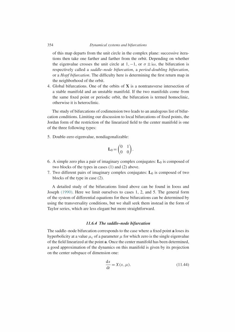
354 Dynamical systems and bifurcations

of this map departs from the unit circle in the complex plane: successive itera-tions then take one farther and farther from the orbit. Depending on whetherthe eigenvalue crosses the unit circle at 1,−1, or σ ± iω, the bifurcation isrespectively called a saddle–node bifurcation, a period-doubling bifurcation,or a Hopf bifurcation. The difficulty here is determining the first return map inthe neighborhood of the orbit.

4. Global bifurcations. One of the orbits of X is a nontransverse intersection ofa stable manifold and an unstable manifold. If the two manifolds come fromthe same fixed point or periodic orbit, the bifurcation is termed homoclinic,otherwise it is heteroclinic.

The study of bifurcations of codimension two leads to an analogous list of bifur-cation conditions. Limiting our discussion to local bifurcations of fixed points, theJordan form of the restriction of the linearized field to the center manifold is oneof the three following types:

5. Double-zero eigenvalue, nondiagonalizable:

L0 =(

0 10 0

).

6. A simple zero plus a pair of imaginary complex conjugates: L0 is composed oftwo blocks of the types in cases (1) and (2) above.

7. Two different pairs of imaginary complex conjugates: L0 is composed of twoblocks of the type in case (2).

A detailed study of the bifurcations listed above can be found in Iooss andJoseph (1990). Here we limit ourselves to cases 1, 2, and 5. The general formof the system of differential equations for these bifurcations can be determined byusing the transversality conditions, but we shall seek them instead in the form ofTaylor series, which are less elegant but more straightforward.

11.6.4 The saddle–node bifurcation

The saddle–node bifurcation corresponds to the case where a fixed point a loses itshyperbolicity at a value µc of a parameter µ for which zero is the single eigenvalueof the field linearized at the point a. Once the center manifold has been determined,a good approximation of the dynamics on this manifold is given by its projectionon the center subspace of dimension one:

dx

dt= X (x,µ). (11.44)

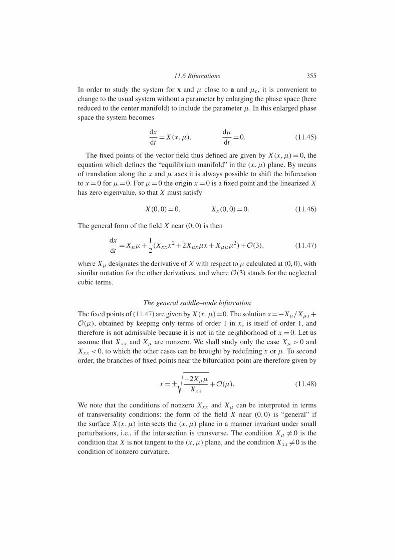
11.6 Bifurcations 355

In order to study the system for x and µ close to a and µc, it is convenient tochange to the usual system without a parameter by enlarging the phase space (herereduced to the center manifold) to include the parameter µ. In this enlarged phasespace the system becomes

dx

dt= X (x,µ),

dµ

dt=0. (11.45)

The fixed points of the vector field thus defined are given by X (x,µ)= 0, theequation which defines the “equilibrium manifold” in the (x,µ) plane. By meansof translation along the x and µ axes it is always possible to shift the bifurcationto x =0 for µ= 0. For µ= 0 the origin x =0 is a fixed point and the linearized Xhas zero eigenvalue, so that X must satisfy

X (0,0)=0, Xx (0,0)=0. (11.46)

The general form of the field X near (0,0) is then

dx

dt= Xµµ+ 1

2(Xxx x2 +2Xµxµx + Xµµµ

2)+O(3), (11.47)

where Xµ designates the derivative of X with respect to µ calculated at (0,0), withsimilar notation for the other derivatives, and where O(3) stands for the neglectedcubic terms.

The general saddle–node bifurcation

The fixed points of (11.47) are given by X (x,µ)=0. The solution x =−Xµ/Xµx +O(µ), obtained by keeping only terms of order 1 in x , is itself of order 1, andtherefore is not admissible because it is not in the neighborhood of x = 0. Let usassume that Xxx and Xµ are nonzero. We shall study only the case Xµ > 0 andXxx < 0, to which the other cases can be brought by redefining x or µ. To secondorder, the branches of fixed points near the bifurcation point are therefore given by

x =±√

−2Xµµ

Xxx+O(µ). (11.48)

We note that the conditions of nonzero Xxx and Xµ can be interpreted in termsof transversality conditions: the form of the field X near (0,0) is “general” ifthe surface X (x,µ) intersects the (x,µ) plane in a manner invariant under smallperturbations, i.e., if the intersection is transverse. The condition Xµ = 0 is thecondition that X is not tangent to the (x,µ) plane, and the condition Xxx =0 is thecondition of nonzero curvature.

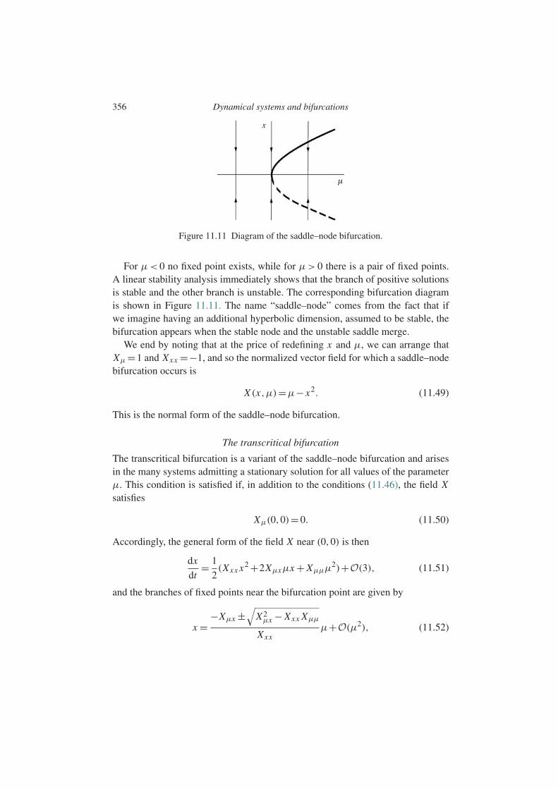
356 Dynamical systems and bifurcations

Figure 11.11 Diagram of the saddle–node bifurcation.

For µ< 0 no fixed point exists, while for µ> 0 there is a pair of fixed points.A linear stability analysis immediately shows that the branch of positive solutionsis stable and the other branch is unstable. The corresponding bifurcation diagramis shown in Figure 11.11. The name “saddle–node” comes from the fact that ifwe imagine having an additional hyperbolic dimension, assumed to be stable, thebifurcation appears when the stable node and the unstable saddle merge.

We end by noting that at the price of redefining x and µ, we can arrange thatXµ =1 and Xxx =−1, and so the normalized vector field for which a saddle–nodebifurcation occurs is

X (x,µ)=µ− x2. (11.49)

This is the normal form of the saddle–node bifurcation.

The transcritical bifurcation

The transcritical bifurcation is a variant of the saddle–node bifurcation and arisesin the many systems admitting a stationary solution for all values of the parameterµ. This condition is satisfied if, in addition to the conditions (11.46), the field Xsatisfies

Xµ(0,0)=0. (11.50)

Accordingly, the general form of the field X near (0,0) is then

dx

dt= 1

2(Xxx x2 +2Xµxµx + Xµµµ

2)+O(3), (11.51)

and the branches of fixed points near the bifurcation point are given by

x =−Xµx ±

√X2

µx − Xxx Xµµ

Xxxµ+O(µ2), (11.52)

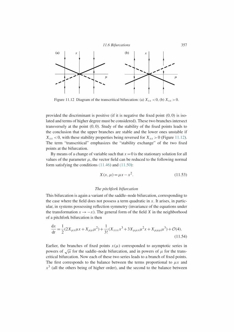
11.6 Bifurcations 357

Figure 11.12 Diagram of the transcritical bifurcation: (a) Xxx <0, (b) Xxx >0.

provided the discriminant is positive (if it is negative the fixed point (0,0) is iso-lated and terms of higher degree must be considered). These two branches intersecttransversely at the point (0,0). Study of the stability of the fixed points leads tothe conclusion that the upper branches are stable and the lower ones unstable ifXxx <0, with these stability properties being reversed for Xxx >0 (Figure 11.12).The term “transcritical” emphasizes the “stability exchange” of the two fixedpoints at the bifurcation.

By means of a change of variable such that x =0 is the stationary solution for allvalues of the parameter µ, the vector field can be reduced to the following normalform satisfying the conditions (11.46) and (11.50):

X (x,µ)=µx − x2. (11.53)

The pitchfork bifurcation

This bifurcation is again a variant of the saddle–node bifurcation, corresponding tothe case where the field does not possess a term quadratic in x . It arises, in partic-ular, in systems possessing reflection symmetry (invariance of the equations underthe transformation x →−x). The general form of the field X in the neighborhoodof a pitchfork bifurcation is then

dx

dt= 1

2(2Xµxµx + Xµµµ

2)+ 1

3!(Xxxx x3 +3Xµµxµ

2x + Xµµµµ3)+O(4).

(11.54)

Earlier, the branches of fixed points x(µ) corresponded to asymptotic series inpowers of

√µ for the saddle–node bifurcation, and in powers of µ for the trans-

critical bifurcation. Now each of these two series leads to a branch of fixed points.The first corresponds to the balance between the terms proportional to µx andx3 (all the others being of higher order), and the second to the balance between

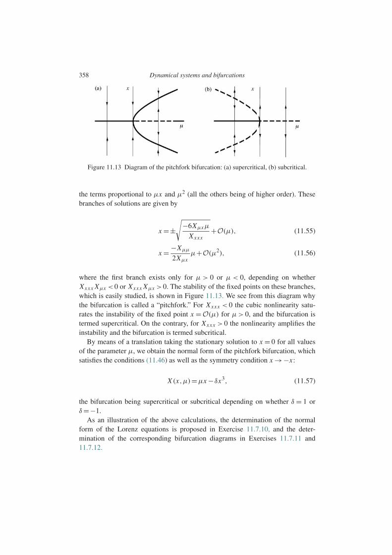
358 Dynamical systems and bifurcations

Figure 11.13 Diagram of the pitchfork bifurcation: (a) supercritical, (b) subcritical.

the terms proportional to µx and µ2 (all the others being of higher order). Thesebranches of solutions are given by

x =±√

−6Xµxµ

Xxxx+O(µ), (11.55)

x = −Xµµ

2Xµxµ+O(µ2), (11.56)

where the first branch exists only for µ > 0 or µ < 0, depending on whetherXxxx Xµx <0 or Xxxx Xµx >0. The stability of the fixed points on these branches,which is easily studied, is shown in Figure 11.13. We see from this diagram whythe bifurcation is called a “pitchfork.” For Xxxx < 0 the cubic nonlinearity satu-rates the instability of the fixed point x =O(µ) for µ> 0, and the bifurcation istermed supercritical. On the contrary, for Xxxx > 0 the nonlinearity amplifies theinstability and the bifurcation is termed subcritical.

By means of a translation taking the stationary solution to x = 0 for all valuesof the parameter µ, we obtain the normal form of the pitchfork bifurcation, whichsatisfies the conditions (11.46) as well as the symmetry condition x →−x :

X (x,µ)=µx −δx3, (11.57)

the bifurcation being supercritical or subcritical depending on whether δ = 1 orδ=−1.

As an illustration of the above calculations, the determination of the normalform of the Lorenz equations is proposed in Exercise 11.7.10, and the deter-mination of the corresponding bifurcation diagrams in Exercises 11.7.11 and11.7.12.

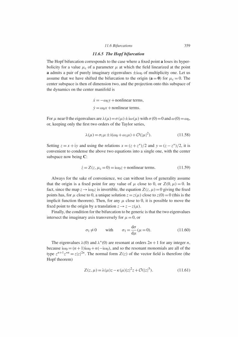
11.6 Bifurcations 359

11.6.5 The Hopf bifurcation

The Hopf bifurcation corresponds to the case where a fixed point a loses its hyper-bolicity for a value µc of a parameter µ at which the field linearized at the pointa admits a pair of purely imaginary eigenvalues ±iω0 of multiplicity one. Let usassume that we have shifted the bifurcation to the origin (a = 0) for µc = 0. Thecenter subspace is then of dimension two, and the projection onto this subspace ofthe dynamics on the center manifold is

x =−ω0y +nonlinear terms,

y =ω0x +nonlinear terms.

For µ near 0 the eigenvalues are λ(µ)=σ(µ)±iω(µ) with σ(0)=0 and ω(0)=ω0,or, keeping only the first two orders of the Taylor series,

λ(µ)=σ1µ± i(ω0 +ω1µ)+O(|µ|2). (11.58)

Setting z = x + iy and using the relations x = (z + z∗)/2 and y = (z − z∗)/2, it isconvenient to condense the above two equations into a single one, with the centersubspace now being C:

z = Z(z,µc =0)= iω0z +nonlinear terms. (11.59)

Always for the sake of convenience, we can without loss of generality assumethat the origin is a fixed point for any value of µ close to 0, or Z(0,µ) = 0. Infact, since the map z → iω0z is invertible, the equation Z(z,µ)=0 giving the fixedpoints has, for µ close to 0, a unique solution z = z(µ) close to z(0)=0 (this is theimplicit function theorem). Then, for any µ close to 0, it is possible to move thefixed point to the origin by a translation z → z − z(µ).

Finally, the condition for the bifurcation to be generic is that the two eigenvaluesintersect the imaginary axis transversely for µ=0, or

σ1 =0 with σ1 = dσ

dµ(µ=0). (11.60)

The eigenvalues λ(0) and λ∗(0) are resonant at orders 2n +1 for any integer n,because iω0 = (n +1)iω0 +n(−iω0), and so the resonant monomials are all of thetype zn+1z∗n = z|z|2n . The normal form Z(z) of the vector field is therefore (theHopf theorem)

Z(z,µ)=λ(µ)z −κ(µ)|z|2z +O(|z|5). (11.61)

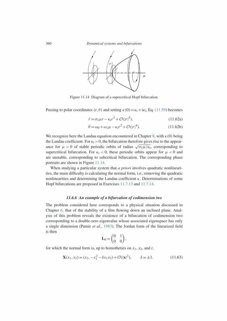
360 Dynamical systems and bifurcations

Figure 11.14 Diagram of a supercritical Hopf bifurcation.

Passing to polar coordinates (r,θ) and setting κ(0)=κr + iκi, Eq. (11.59) becomes

r =σ1µr −κrr3 +O(|r |5), (11.62a)

θ =ω0 +ω1µ−κir2 +O(|r |4). (11.62b)

We recognize here the Landau equation encountered in Chapter 8, with κ(0) beingthe Landau coefficient. For κr>0, the bifurcation therefore gives rise to the appear-ance for µ > 0 of stable periodic orbits of radius

√σ1µ/κr, corresponding to

supercritical bifurcation. For κr < 0, these periodic orbits appear for µ < 0 andare unstable, corresponding to subcritical bifurcation. The corresponding phaseportraits are shown in Figure 11.14.

When studying a particular system that a priori involves quadratic nonlineari-ties, the main difficulty is calculating the normal form, i.e., removing the quadraticnonlinearities and determining the Landau coefficient κ . Determinations of someHopf bifurcations are proposed in Exercises 11.7.13 and 11.7.14.

11.6.6 An example of a bifurcation of codimension two

The problem considered here corresponds to a physical situation discussed inChapter 6, that of the stability of a film flowing down an inclined plane. Anal-ysis of this problem reveals the existence of a bifurcation of codimension twocorresponding to a double-zero eigenvalue whose associated eigenspace has onlya single dimension (Pumir et al., 1983). The Jordan form of the linearized fieldis then

L0 =(

0 10 0

),

for which the normal form is, up to homotheties on x1, x2, and t ,

X(x1, x2)= (x2,−x21 −δx1x2)+O(|x|2), δ=±1. (11.63)

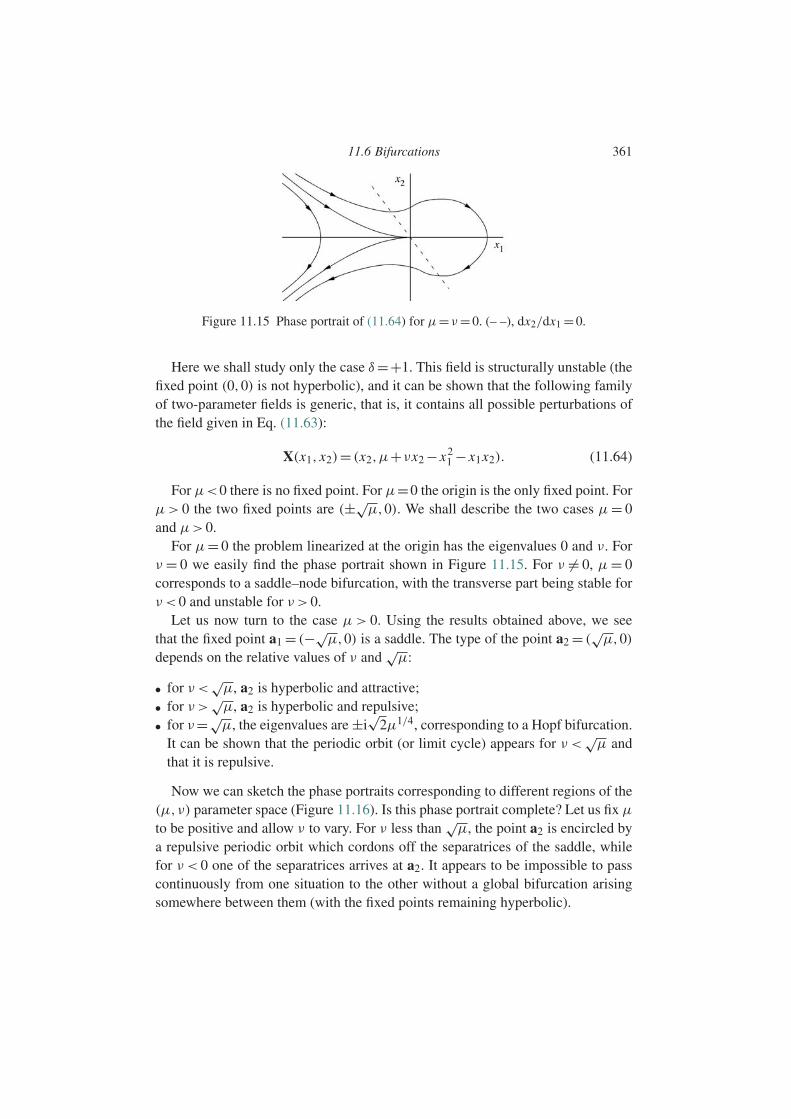
11.6 Bifurcations 361

Figure 11.15 Phase portrait of (11.64) for µ= ν =0. (– –), dx2/dx1 =0.

Here we shall study only the case δ=+1. This field is structurally unstable (thefixed point (0,0) is not hyperbolic), and it can be shown that the following familyof two-parameter fields is generic, that is, it contains all possible perturbations ofthe field given in Eq. (11.63):

X(x1, x2)= (x2,µ+νx2 − x21 − x1x2). (11.64)

For µ<0 there is no fixed point. For µ=0 the origin is the only fixed point. Forµ> 0 the two fixed points are (±√

µ,0). We shall describe the two cases µ= 0and µ>0.

For µ= 0 the problem linearized at the origin has the eigenvalues 0 and ν. Forν = 0 we easily find the phase portrait shown in Figure 11.15. For ν = 0, µ= 0corresponds to a saddle–node bifurcation, with the transverse part being stable forν <0 and unstable for ν >0.

Let us now turn to the case µ> 0. Using the results obtained above, we seethat the fixed point a1 = (−√

µ,0) is a saddle. The type of the point a2 = (√µ,0)

depends on the relative values of ν and√µ:

• for ν <√µ, a2 is hyperbolic and attractive;

• for ν >√µ, a2 is hyperbolic and repulsive;

• for ν=√µ, the eigenvalues are ±i

√2µ1/4, corresponding to a Hopf bifurcation.

It can be shown that the periodic orbit (or limit cycle) appears for ν <√µ and

that it is repulsive.

Now we can sketch the phase portraits corresponding to different regions of the(µ,ν) parameter space (Figure 11.16). Is this phase portrait complete? Let us fix µ

to be positive and allow ν to vary. For ν less than√µ, the point a2 is encircled by

a repulsive periodic orbit which cordons off the separatrices of the saddle, whilefor ν < 0 one of the separatrices arrives at a2. It appears to be impossible to passcontinuously from one situation to the other without a global bifurcation arisingsomewhere between them (with the fixed points remaining hyperbolic).

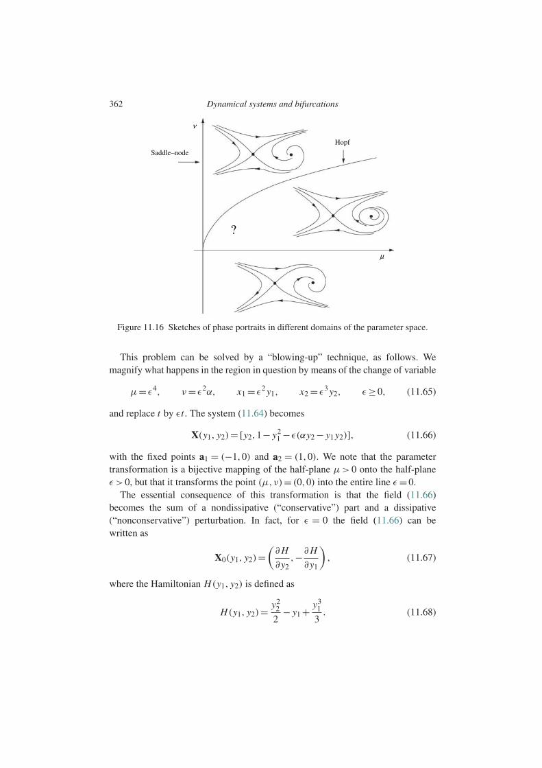
362 Dynamical systems and bifurcations

Saddle–node

ν

Hopf

?

µ

Figure 11.16 Sketches of phase portraits in different domains of the parameter space.

This problem can be solved by a “blowing-up” technique, as follows. Wemagnify what happens in the region in question by means of the change of variable

µ= ε4, ν = ε2α, x1 = ε2y1, x2 = ε3y2, ε ≥0, (11.65)

and replace t by εt . The system (11.64) becomes

X(y1, y2)= [y2,1− y21 −ε(αy2 − y1y2)], (11.66)

with the fixed points a1 = (−1,0) and a2 = (1,0). We note that the parametertransformation is a bijective mapping of the half-plane µ> 0 onto the half-planeε >0, but that it transforms the point (µ,ν)= (0,0) into the entire line ε =0.

The essential consequence of this transformation is that the field (11.66)becomes the sum of a nondissipative (“conservative”) part and a dissipative(“nonconservative”) perturbation. In fact, for ε = 0 the field (11.66) can bewritten as

X0(y1, y2)=(∂H

∂y2,−∂H

∂y1

), (11.67)

where the Hamiltonian H(y1, y2) is defined as

H(y1, y2)=y2

2

2− y1 + y3

1

3. (11.68)

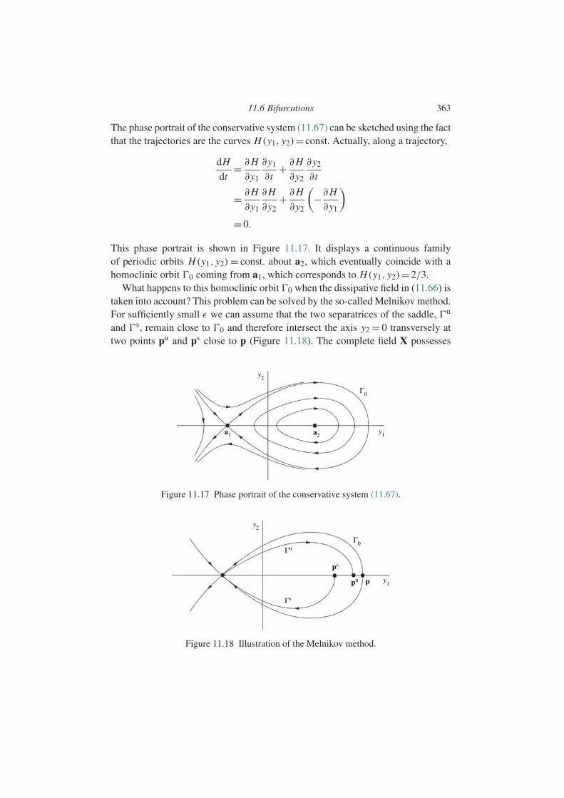
11.6 Bifurcations 363

The phase portrait of the conservative system (11.67) can be sketched using the factthat the trajectories are the curves H(y1, y2)= const. Actually, along a trajectory,

dH

dt= ∂H

∂y1

∂y1

∂t+ ∂H

∂y2

∂y2

∂t

= ∂H

∂y1

∂H

∂y2+ ∂H

∂y2

(−∂H

∂y1

)=0.

This phase portrait is shown in Figure 11.17. It displays a continuous familyof periodic orbits H(y1, y2)= const. about a2, which eventually coincide with ahomoclinic orbit 0 coming from a1, which corresponds to H(y1, y2)=2/3.

What happens to this homoclinic orbit 0 when the dissipative field in (11.66) istaken into account? This problem can be solved by the so-called Melnikov method.For sufficiently small ε we can assume that the two separatrices of the saddle, u

and s, remain close to 0 and therefore intersect the axis y2 = 0 transversely attwo points pu and ps close to p (Figure 11.18). The complete field X possesses

y2

y1

Γ0

a2a1

Figure 11.17 Phase portrait of the conservative system (11.67).

y2

ps

pu p y1

Γ0

Γs

Γu

Figure 11.18 Illustration of the Melnikov method.

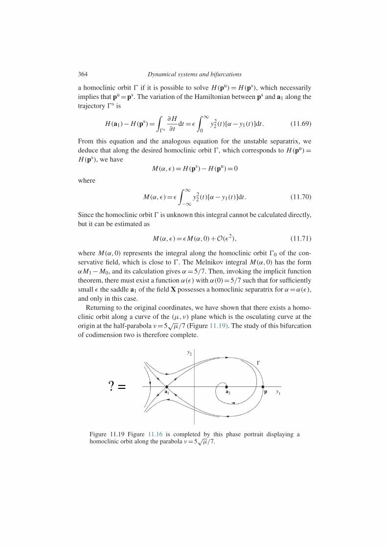
364 Dynamical systems and bifurcations

a homoclinic orbit if it is possible to solve H(pu)= H(ps), which necessarilyimplies that pu =ps. The variation of the Hamiltonian between ps and a1 along thetrajectory s is

H(a1)− H(ps)=∫s

∂H

∂tdt = ε

∫ ∞

0y2

2(t)[α− y1(t)]dt. (11.69)

From this equation and the analogous equation for the unstable separatrix, wededuce that along the desired homoclinic orbit , which corresponds to H(pu)=H(ps), we have

M(α,ε)= H(ps)− H(pu)=0

where

M(α,ε)= ε

∫ ∞

−∞y2

2(t)[α− y1(t)]dt. (11.70)

Since the homoclinic orbit is unknown this integral cannot be calculated directly,but it can be estimated as

M(α,ε)= εM(α,0)+O(ε2), (11.71)

where M(α,0) represents the integral along the homoclinic orbit 0 of the con-servative field, which is close to . The Melnikov integral M(α,0) has the formαM1 − M0, and its calculation gives α=5/7. Then, invoking the implicit functiontheorem, there must exist a function α(ε) with α(0)=5/7 such that for sufficientlysmall ε the saddle a1 of the field X possesses a homoclinic separatrix for α=α(ε),and only in this case.

Returning to the original coordinates, we have shown that there exists a homo-clinic orbit along a curve of the (µ,ν) plane which is the osculating curve at theorigin at the half-parabola ν=5

õ/7 (Figure 11.19). The study of this bifurcation

of codimension two is therefore complete.

? = a1 a2 y1p

y2

Γ

Figure 11.19 Figure 11.16 is completed by this phase portrait displaying ahomoclinic orbit along the parabola ν =5

õ/7.

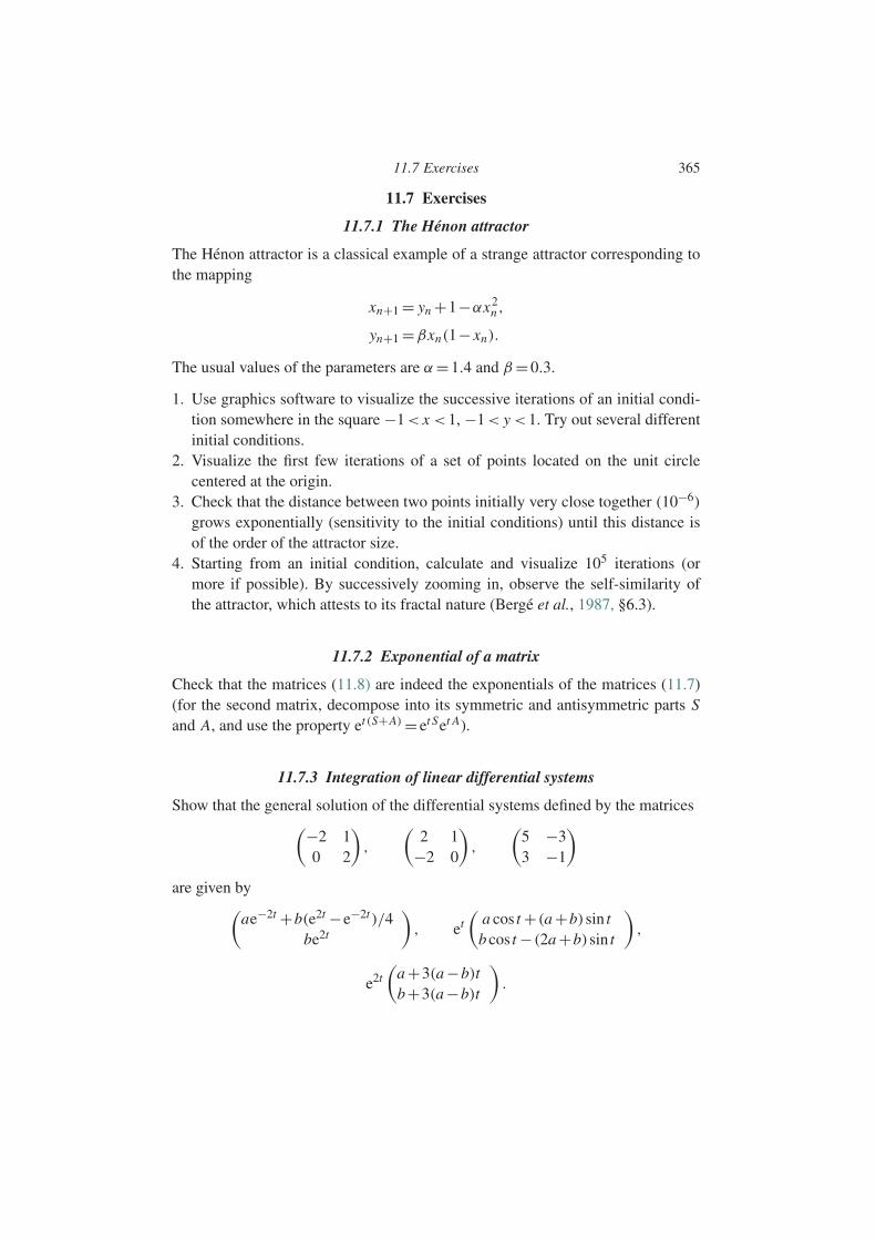
11.7 Exercises 365

11.7 Exercises

11.7.1 The Henon attractor

The Henon attractor is a classical example of a strange attractor corresponding tothe mapping

xn+1 = yn +1−αx2n ,

yn+1 =βxn(1− xn).

The usual values of the parameters are α=1.4 and β =0.3.

1. Use graphics software to visualize the successive iterations of an initial condi-tion somewhere in the square −1< x <1, −1< y <1. Try out several differentinitial conditions.

2. Visualize the first few iterations of a set of points located on the unit circlecentered at the origin.

3. Check that the distance between two points initially very close together (10−6)

grows exponentially (sensitivity to the initial conditions) until this distance isof the order of the attractor size.

4. Starting from an initial condition, calculate and visualize 105 iterations (ormore if possible). By successively zooming in, observe the self-similarity ofthe attractor, which attests to its fractal nature (Berge et al., 1987, §6.3).

11.7.2 Exponential of a matrix

Check that the matrices (11.8) are indeed the exponentials of the matrices (11.7)(for the second matrix, decompose into its symmetric and antisymmetric parts Sand A, and use the property et (S+A) = et Set A).

11.7.3 Integration of linear differential systems

Show that the general solution of the differential systems defined by the matrices(−2 10 2

),

(2 1

−2 0

),

(5 −33 −1

)are given by(

ae−2t +b(e2t −e−2t )/4be2t

), et

(a cos t +(a +b)sin tb cos t −(2a +b)sin t

),

e2t(

a +3(a −b)tb+3(a −b)t

).

366 Dynamical systems and bifurcations

11.7.4 The phase portrait

Show that the stable manifold of the example given in Section 11.4.1 is the axisOy. Sketch the phase portrait for a =1 (noting that y =0 on the parabola y = x2).

11.7.5 Stable and unstable manifolds

Determine the stable and unstable manifolds, to third order, for the followingsystems:

x =−3x +2y2 + xy, y =−y +3y2 + x2y −4x3;x =−2x −3y − x2, y = x +2y + xy −3y3.

In each case find the equation of motion on the unstable manifold to second order.

11.7.6 The center manifold

Determine the center manifold and the dynamics on this manifold for the system

x = xy,

y =−y +αx2.

Can this dynamics be determined here by the tangent-space approximation h(x)=0+O(x2)? Sketch the phase portrait about the origin. Solution in Guckenheimerand Holmes (1983, p. 133).

11.7.7 Resonances of eigenvalues

Consider a differential system of dimension two whose linear part has the eigen-values λ1 and λ2. If λ1 = 2 and λ2 = −1, the system is resonant of order4, because λ1 = 2λ1 + 2λ2 (or λ2 = λ1 + 3λ2). From this example, determinewhether the eigenvalues below are resonant. If they are, what is the order of theresonance?

• λ1 =1, λ2 =−1 ;• λ1 =3, λ2 =−1 ;• λ1 =1, λ2 =2 ;• λ1 =α, λ2 =α, α>0 ;• λ1 =α, λ2 =−α, α>0.

11.7 Exercises 367

11.7.8 The normal form

Show that the normal form of the differential system

x = x +o(x, y),

y =−y +o(x, y)

is written as

x = x +αx2y +O(5),

y =−y +βxy2 +O(5).

11.7.9 Structural stability of a heteroclinic orbit

Using arguments similar to those at the end of Section 11.5.3, show that a hetero-clinic orbit joining two saddles is structurally unstable in two dimensions, but maybe structurally stable in higher dimensions. What can be said about a heteroclinicorbit joining a saddle and a node?

11.7.10 The normal form of the Lorenz equations

Calculate the normal form of the Lorenz equations

x =−σ x +σ y,

y =−xz +r x − y,

z = xy −bz

near the fixed point (0,0,0) which becomes nonhyperbolic for r = 1, with σ = 10and b =8/3. Show that r =1 corresponds to a saddle–node bifurcation.

11.7.11 Bifurcation diagram (1)

Determine the bifurcation diagram of the differential system

x = x(x2 −µ)(x2 +µ2 −1).

11.7.12 Bifurcation diagram (2)

Determine the bifurcation diagram of the differential system

x =4x[(x −1)2 −µ−1

].

The solution is given in Figure 11.20.

368 Dynamical systems and bifurcations

Figure 11.20 Bifurcation diagram corresponding to the solution of Exercise 11.7.12.

11.7.13 Hopf bifurcation

Determine the Hopf bifurcations of the system

x = x −ωy − x(x2 + y2),

y =ωx + y − y(x2 + y2)−µ.

11.7.14 Hopf bifurcation of the Lorenz system

Show that the two fixed points symmetric about the origin in the Lorenz systembecome nonhyperbolic for some r in the range [24,25], and that the bifurcation isa subcritical Hopf bifurcation (this rather lengthy computational exercise requirescalculation of the normal form near the fixed point in order to explicitly determinethe Landau coefficient κ of the cubic term).

Appendix A: The Saint-Venant equations

In this appendix we shall derive a system of depth-averaged conservationequations, the classic Saint-Venant equations (de Saint-Venant, 1871), which givea good description of the dynamics of a fluid flow when the spatial scale λ of thevariations in the longitudinal direction x is large compared to the flow depth orthickness, h. These equations do not explicitly involve the nature of the flowingmedium, and so they are valid, under certain conditions stated explicitly below, fora fluid flow either laminar or turbulent, as well as for a granular flow. The equationscan be obtained by two equivalent methods: by depth-averaging the local conser-vation equations in the transverse direction, or by writing down the conservationlaws for a control volume corresponding to a slice of fluid of thickness dx . Herewe shall use the latter method.

A.1 Outflow from a slice of fluid

Let us consider a flow in the x-direction, inclined at an angle θ relative to the hor-izontal, between a bed located at y = yb(x, t), where y is the transverse direction,and a free surface at y = (yb + h)(x, t), where h is the local flow depth (FigureA.1).

We define the control volume as the slice of fluid between the two planes atx and x + dx . At any point on the boundary of the control volume, let n be theexterior normal, u the fluid velocity and w the speed of the boundary. The outflowof a scalar quantity φ across the surface A of the slice is∫

Aφ (u−w) ·ndA.

Since the speed w is zero on the planes at x and x +dx , while the normal velocitiesu ·n and w ·n are equal on the bed as well as on the free surface (the kinematiccondition is equivalent to the condition that these surfaces are impermeable), the

369

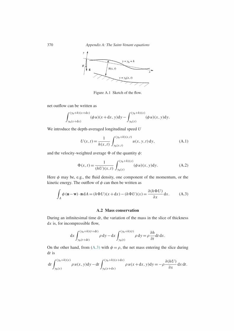
370 Appendix A: The Saint-Venant equations

y

y = yb + h

y = yb(x, t)

h(x, t)gθ

x

Figure A.1 Sketch of the flow.

net outflow can be written as∫ (yb+h)(x+dx)

yb(x+dx)(φ u)(x +dx, y)dy −

∫ (yb+h)(x)

yb(x)(φ u)(x, y)dy.

We introduce the depth-averaged longitudinal speed U

U (x, t)= 1

h(x, t)

∫ (yb+h)(x,t)

yb(x,t)u(x, y, t)dy, (A.1)

and the velocity-weighted average of the quantity φ:

(x, t)= 1

(hU )(x, t)

∫ (yb+h)(x)

yb(x)(φ u)(x, y)dy. (A.2)

Here φ may be, e.g., the fluid density, one component of the momentum, or thekinetic energy. The outflow of φ can then be written as∫

Aφ (u−w) ·ndA = (hU )(x +dx)−(hU )(x)= ∂(hU )

∂xdx . (A.3)

A.2 Mass conservation

During an infinitesimal time dt , the variation of the mass in the slice of thicknessdx is, for incompressible flow,

dx∫ (yb+h)(t+dt)

yb(t+dt)ρ dy −dx

∫ (yb+h)(t)

yb(t)ρ dy =ρ

∂h

∂tdt dx .

On the other hand, from (A.3) with φ = ρ, the net mass entering the slice duringdt is

dt∫ (yb+h)(x)

yb(x)ρ u(x, y)dy −dt

∫ (yb+h)(x+dx)

yb(x+dx)ρ u(x +dx, y)dy =−ρ

∂(hU )

∂xdx dt.

A.3 Momentum conservation 371

Mass conservation implies that the variation of the mass is equal to the net massentering the slice, or

∂h

∂t+ ∂(hU )

∂x=0. (A.4)

A.3 Momentum conservation

Since the longitudinal and transverse velocities, u and v, are such that v∼ (h/λ)uowing to incompressibility, the hypothesis of slow variation in the x-direction, orλh, implies that v is small compared to u. Therefore, it is possible to neglect theinertia and the viscous stresses in the transverse momentum equation (Batchelor,1967, §5.7). The pressure distribution is then hydrostatic in the vertical:

p(x, y, t)= pa +ρg cosθ (yb(x, t)+h(x, t)− y) , (A.5)

where pa is the pressure, assumed to be uniform, above the free surface.The variation of the longitudinal momentum in the control volume during the

time dt is

dx∫ (yb+h)(t+dt)

yb(t+dt)ρu(x, y, t +dt)dy−dx

∫ (yb+h)(t)

yb(t)ρu(x, y, t)dy =ρ

∂(hU )

∂tdt dx .

The momentum entering this volume during the same time is obtained from (A.3)with φ=ρu, which gives

dt∫ (yb+h)(x)

yb(x)(ρu2)(x, y)dy −dt

∫ (yb+h)(x+dx)

yb(x+dx)(ρu2)(x +dx, y)dy =

−ρ∂(cu2hU 2)

∂xdx dt,

where the shape factor

cu2(x, t)= 1

U 2h

∫ (yb+h)(x,t)

yb(x,t)u2(x, y, t)dy (A.6)

corresponds to =ρcu2U in (A.3). This coefficient depends on the velocity pro-file, which is generally unknown. A simplification is commonly made here, whichconsists of assuming a particular velocity profile. In particular:

• cu2 =1 for a uniform velocity profile u(y)=U , which, however crude, is a widelyused approximation for turbulent flows at large Reynolds number.

• cu2 = 4/3 for the linear velocity profile u(y) = γ y of sheared films or certaingranular flows (Rajchenbach, 2000).

372 Appendix A: The Saint-Venant equations

• cu2 = 5/4 for the Bagnold velocity profile u(y) ∼ y3/2 of a granular flow(Bagnold, 1956).

• cu2 = 6/5 for the semi-parabolic profile corresponding to a falling viscous filmu(y)=Umax(y/h)(2− y/h), where Umax = 3

2U is the speed of the free surface.

In any case, we see that the shape factor does not vary much and is a constant oforder unity. If the relaxation time of the flow over the flow depth is short comparedto the other time scales, the velocity profile is nearly fully developed, and thecoefficient cu2 can be considered as constant, with error of the order of the smallgradient parameter h/λ.

Taking into account the hydrostatic pressure distribution (A.5), and neglect-ing terms of order (h/λ)2, the longitudinal momentum flux associated with thepressure forces is∫ (yb+h)(x)

yb(x)p(x, y)dy −

∫ (yb+h)(x+dx)

yb(x+dx)p(x +dx, y)dy+

+ pa(x, yb +h)dx ∂x (yb +h)

− p(x, yb)dx ∂x yb =dx ρgh cosθ ∂x (yb +h)

(the pressure pa vanishes upon integration). The momentum flux associated withthe viscous stresses is nonzero only on the bed (when the normal viscous stressescan be neglected) and equal to −τdx per unit time, where τ is the tangentialstress exerted by the fluid on the bed. Finally, the flux associated with gravityis ρgh sinθ dx .

Therefore, assuming constant shape factor cu2 , the final form of the depth-averaged momentum equation is

∂(Uh)

∂t+cu2

∂(U 2h)

∂x=−gh cosθ

∂(yb +h)

∂x− τ

ρ+gh sinθ. (A.7)

This equation, together with the mass conservation equation (A.4), constitutes theSaint-Venant equations. For turbulent flow, the additional approximation cu2 = 1allows a further simplification of the left-hand side: using mass conservation (A.4),the above equation becomes

h∂U

∂t+Uh

∂U

∂x=−gh cosθ

∂(yb +h)

∂x− τ

ρ+gh sinθ. (A.8)

A.4 Modeling the wall friction

The Saint-Venant equations involve the unknown wall shear, which must be mod-eled, that is, expressed as a function of the averages U and h, in order to result in

A.5 Consistent depth-averaged equations 373

a closed set of equations. This is where we encounter the second major difficulty(after the problem of the shape factor) in accurately representing the physics of theproblem. Here we shall give the classical closure relations for three types of flow:a viscous film, a flow at large Reynolds number, and a granular flow.

• For a viscous film, the hypothesis of a fully developed profile, that is, a parabolicprofile (cu2 =6/5 uniform) leads to

τ =µ∂u

∂y(yb)=µ

2Umax

h=µ

3U

h= 3µ

QU 2, (A.9)

where Q =Uh is the flow volume per unit width.• For flows at large Reynolds number, the shear is classically related to the speed

U by a friction coefficient cf defined as

τ = cfρU 2

2. (A.10)

This friction coefficient depends on the Reynolds number Re = ρUh/µ andthe dimensionless bed roughness z0/h. For turbulent flow on smooth walls, arelation often used in hydraulics is the empirical Blasius relation (Pope, 2000):

cf =0.316Re−1/4, (A.11)

while for rough walls, a widely used expression is that of Manning–Strickler:

cf =0.1( z0

h

)1/3. (A.12)

More complex relations involving both Re and z0/h, or the logarithmic velocityprofile, are also available.

• For a dry granular flow the shear can be related to the normal stress ρgh by aCoulomb friction coefficient µf:

τ =µf ρgh. (A.13)

This coefficient can be assumed to be constant (Savage and Hutter, 1989), orrelated to the speed and thickness of the flow by a phenomenological relationµf =µf(U,h) (Pouliquen, 1999).

A.5 Consistent depth-averaged equations

Finally, it must be stressed that the Saint-Venant equations are not a consis-tent approximation of the Navier–Stokes equations, in the sense that they do notaccount correctly for first-order corrections in the small parameter h/λ. Thus, the

374 Appendix A: The Saint-Venant equations

use of these equations for stability calculations is questionable, at least when seek-ing quantitative predictions. A consistent set of depth-averaged equations basednot on the momentum equation but on the kinetic energy equation has beendeveloped recently (Luchini and Charru, 2010a, 2010b). These give the correctquantitative predictions of stability.

References

Abramowitz, M. and Stegun, I. A. (1964) Handbook of Mathematical Functions withFormulas, Graphs, and Mathematical Tables. New York: Dover.

Abrams, J. and Hanratty, T. J. (1985) Relaxation effects observed for turbulent flow over awavy surface. J. Fluid Mech. 151, 443–55.

Acheson, D. J. (1990) Elementary Fluid Dynamics. Oxford: Clarendon Press.Andersen, K. H. (2001) A particle model of rolling grain ripples under waves. Phys. Fluids

13(1), 58–64.Andreotti, B. (2004) A two species model for aeolian sand transport. J. Fluid Mech. 510,

47–70.Andreotti, B., Claudin, P. and Douady, S. (2002a) Selection of dune shapes and velocities.

Part 1: dynamics of sand, wind and barchans. Eur. Phys. J. B 28, 321–39.Andreotti, B., Claudin, P. and Douady, S. (2002b) Selection of dune shapes and velocities.

Part 2: a two-dimensional modelling. Eur. Phys. J. B 28, 341–52.Anshus, B. E. and Goren, S. L. (1966) A method of getting approximate solutions of the

Orr–Sommerfeld equation for flow on a vertical wall. AIChE J. 12, 1004–8.Aradian, A., Raphael, E. and de Gennes, P. G. (2002) Surface flows of granular materials:

a short introduction to some recent models. C.R. Physique 3(2), 187–96.Aranson, I. S. and Tsimring, L. S. (2006) Patterns and collective behavior in granular

media: Theoretical concepts. Rev. Mod. Phys. 78, 641–92.Arnal, D. (1994) Predictions based on linear theory. AGARD Rep. 793. ONERA.Arnold, V. I. (1973) Ordinary Differential Equations. Cambridge, MA: MIT Press.ASCE Task Committee on Flow and Transport over Dunes (2002) Flow and transport over

dunes. J. Hydr. Engrg. 128(8), 726–8.Ayrton, H. (1910) The origin and growth of ripple-mark. Proc. R. Soc. Lond. A 84, 285–

310.Bagnold, R. A. (1941) The Physics of Blown Sand and Desert Dunes. London: Chapman

& Hall.Bagnold, R. A. (1946) Motion of waves in shallow water. interaction between waves and

sand bottoms. Proc. R. Soc. Lond. A 187, 1–18.Bagnold, R. A. (1954) Experiments on a gravity-free dispersion of large solid spheres in a

Newtonian fluid under shear, Proc. R. Soc. Lond. A 225, 49–63.Bagnold, R. A. (1956) The flow of cohesionless grains in fluids. Phil. Trans. R. Soc. Lond.

A 249, 235–97.Bagnold, R. A. (1973) The nature of saltation and of ‘bed-load’ transport in water. Proc. R.

Soc. Lond. A 332, 473–504.

375

376 References

Baines, P. G., Majumdar, S. and Mitsudera, H. (1996) The mechanics of the Tollmien–Schlichting wave. J. Fluid Mech. 312, 107–24.

Barthelet, P. and Charru, F. (1998) Benjamin–Feir and Eckhaus instabilities with Galileaninvariance: the case of interfacial waves in viscous shear flows. Eur. J. Mech. B 17(1),1–18.

Barthelet, P., Charru, F. and Fabre, J. (1995) Experimental study of interfacial long wavesin a two-layer shear flow. J. Fluid Mech. 303, 23–53.

Batchelor, G. K. (1967) An Introduction to Fluid Dynamics. Cambridge: CambridgeUniversity Press.

Bayly, B. J., Orszag, S. A. and Herbert, T. (1988) Instability mechanisms in shear-flowtransition. Annu. Rev. Fluid Mech. 20, 359–91.

Benard, H. (1900) Les tourbillons cellulaires dans une nappe liquide. Revue Gen. Sci. PuresAppl. 11, 1261–71, 1309–28.

Bender, C. M. and Orszag, S. A. (1978) Advanced Mathematical Methods for Scientistsand Engineers. New York: McGraw-Hill.

Benjamin, T. B. (1957) Wave formation in laminar flow down an inclined plane. J. FluidMech. 2, 554–74.

Benjamin, T. B. (1959) Shearing flow over a wavy boundary. J. Fluid Mech. 6, 161–205.Benjamin, T. B. and Feir, J. E. (1967) The disintegration of wave trains on deep water.

J. Fluid Mech. 27, 417–30.Benjamin, T. B. and Hasselmann, K. (1967) Instability of periodic wavetrains in nonlinear

dispersive systems. Proc. R. Soc. Lond. A 299(1456), 59–76.Benjamin, T. B. and Ursell, F. (1954) The stability of the plane free surface of liquid in

vertical periodic motion. Proc. R. Soc. Lond. A 225, 505–15.Benney, D. J. (1966) Long waves on liquid films. J. Math. Phys. 45, 150–55.Benney, D. J. and Newell, A. C. (1967) The propagation of non-linear wave envelopes.

J. Math. Phys. 46, 133–45.Berge, P., Pomeau, Y. and Vidal, C. (1987) Order Within Chaos: Towards a Deterministic

Approach to Turbulence. New York: John Wiley & Sons.Betchov, R. and Szewczyk, A. (1963) Stability of a shear layer between parallel streams.

Phys. Fluids 6, 1391–6.Billingham, J. and King, A. C. (2000) Wave Motion. Cambridge: Cambridge University

Press.Binney, J. and Tremaine, S. (1988) Galactic Dynamics. Princeton, NJ: Princeton University

Press.Blondeaux, P. (1990) Sand ripples under sea waves. Part 1. Ripple formation. J. Fluid

Mech. 218, 1–17.Blondeaux, P. (2001) Mechanics of coastal forms. Annu. Rev. Fluid Mech. 33, 339–70.Bogolioubov, N. and Mitropolski, I. (1962) Les methodes asymptotiques en theorie des

oscillations non lineaires. Paris: Gauthier-Villars.Bottaro, A. and Luchini, P. (1999) Gortler vortices: are they amenable to local eigenvalue

analysis. Eur. J. Mech. B/Fluids 18(1), 47–65.Bouasse, H. (1924) Houle, rides, seiches et marees. In Bibliotheque scientifique de

l’ingenieur et du physicien. Paris: Delagrave.Boussinesq, J. (1871) Theorie de l’intumescence liquide, appelee onde solitaire ou de

translation, se propageant dans un canal rectangulaire. C. R. Acad. Sci. Paris 72, 755–9.Busse, F. and Whitehead, J. A. (1971) Instabilities of convection rolls in a high Prandtl

number fluid. J. Fluid Mech. 47, 305–20.Butler, K. M. and Farrell, B. F. (1992) Three-dimensional optimal perturbations in viscous

shear flow. Phys. Fluids A 4(8), 1637–50.

References 377

Callen, H. B. (1985) Thermodynamics and an Introduction to Thermostatistics. New York:John Wiley & Sons.

Canuto, C., Hussaini, M. Y., Quarteroni, A. and Zang, T. A. (1988) Spectral Methods inFluid Dynamics. New York: Springer-Verlag.

Case, K. M. (1960) Stability of inviscid plane Couette flow. Phys. Fluids 3, 143–8.Chandrasekhar, S. (1961) Hydrodynamic and Hydromagnetic Stability. New York: Dover.Chang, H.-C. (1994) Wave evolution on a falling film. Annu. Rev. Fluid Mech. 26, 103–36.Charru, F. (1997) A simple mechanical system mimicking phase transitions in a one-

dimensional medium. Eur. J. Phys. 18, 417–24.Charru, F. (2006) Selection of the ripple length on a granular bed sheared by a liquid flow.

Phys. Fluids 18, 121508.Charru, F. and Barthelet, P. (1999) Secondary instabilities of interfacial waves due to

coupling with a long wave mode in a two-layer Couette flow. Physica D 125, 311–24.Charru, F. and Hinch, E. J. (2000) ‘Phase diagram’ of interfacial instabilites in a two-

layer Couette flow and mechanism for the long-wave instability. J. Fluid Mech. 414,195–223.

Charru, F. and Hinch, E. J. (2006) Ripple formation on a particle bed sheared by a viscousliquid. Part 2. Oscillating flow. J. Fluid Mech. 550, 123–37.

Charru, F., Larrieu, E., Dupont, J.-B. and Zenit, R. (2007) Motion of a particle near a roughwall in a viscous shear flow. J. Fluid Mech. 570, 431–53.

Charru, F., Mouilleron, H. and Eiff, O. (2004) Erosion and deposition of particles on a bedsheared by a viscous flow. J. Fluid Mech. 519, 55–80.

Charru, F. and Mouilleron-Arnould, H. (2002) Instability of a bed of particles sheared bya viscous flow. J. Fluid Mech. 452, 303–23.

Chavanis, P. H. (2002) Gravitational instability of finite isothermal spheres. Astron.Astrophy. 381, 340–56.

Chomaz, J.-M. (2005) Global instabilities in spatially developing flows: non-normality andnonlinearity. Annu. Rev. Fluid Mech. 37, 357–92.

Chossat, P. and Iooss, G. (1994) The Couette–Taylor Problem. Applied MathematicsSeries, Vol. 102. New York: Springer-Verlag.

Clanet, C. and Searby, G. (1998) First experimental study of the Darrieus–Landauinstability. Phys. Rev. Lett. 80, 3867–70.

Coleman, S. E. and Eling, B. (2000) Sand wavelets in laminar open-channel flows.J. Hydraul. Res. 38(5), 331–8.

Coleman, S. E. and Melville, B. W. (1994) Bed-form development. J. Hydr. Engrg. 120(4),544–60.

Coleman, S. E. and Melville, B. W. (1996) Initiation of bed forms on a flat sand bed.J. Hydr. Engrg. 122(6), 301–10.

Colombini, M. (2004) Revisiting the linear theory of sand dune formation. J. Fluid Mech.502, 1–16.

Couder, Y. (2000) Viscous fingering as an archetype for growth patterns. In Perspectives inFluid Mechanics, a Collective Introduction to Current Research (ed. G. K. Batchelor).Paris: Lavoisier.

Couette, M. (1890) Etudes sur le frottement des liquides. Ann. Chim. Phys. 21(6), 433–510.Coullet, P. and Fauve, S. (1985) Propagative phase dynamics for systems with Galilean

invariance. Phys. Rev. Lett. 55, 2857–9.Coullet, P. and Iooss, G. (1990) Instabilities of one-dimensional cellular patterns. Phys.

Rev. Lett. 64(8), 866–9.Cousteix, J. and Mauss, J. (2006) Analyse asymptotique et couche limite. Mathematiques &

Applications, Vol. 56. Berlin: Springer-Verlag.

378 References

Craik, A. D. D. (1985) Wave Interactions and Fluid Flows. Cambridge: CambridgeUniversity Press.

Craik, A. D. D. (2004) The origins of water wave theory. Annu. Rev. Fluid Mech. 36,1–28.

Craik, A. D. D. (2005) George Gabriel Stokes on water wave theory. Annu. Rev. FluidMech. 37, 23–42.

Crawford, J. D. (1991) Introduction to bifurcation theory. Rev. Mod. Phys. 63(4), 991–1037.

Crawford, J. D. and Knobloch, E. (1991) Symmetry and symmetry-breaking bifurcationsin fluid mechanics. Annu. Rev. Fluid Mech. 23, 341–87.

Cross, M. C. and Hohenberg, P. C. (1993) Pattern formation outside of equilibrium. Rev.Mod. Phys. 65(3), 851–1113.

Darrieus, G. (1938) Propagation d’un front de flamme: essai de theorie des vitesses anor-males de deflagration par developpement spontane de la turbulence. Travail non publiepresente a La Technique Moderne, Paris.

Darrigol, O. (2003) The spirited horse, the engineer, and the mathematician: water wavesin nineteenth-century hydrodynamics. Arch. Hist. Exact Sci. 58, 21–95.

Darrigol, O. (2005) Worlds of Flow – A history of hydrodynamics from the Bernoullis toPrandtl. Oxford: Oxford University Press.

Dauxois, T. and Peyrard, M. (2006) Physis of Solitons. Cambridge: Cambridge UniversityPress.

Denn, M. M. (2001) Extrusion instabilities and wall slip. Annu. Rev. Fluid Mech. 33,265–87.

Dias, F. and Kharif, C. (1999) Nonlinear gravity and capillary-gravity waves. Annu. Rev.Fluid Mech. 31, 301–46.

Donnelly, R. J. and Glaberson, W. (1966) Experiments on the capillary instability of aliquid jet. Proc. R. Soc. Lond. A 290, 547–56.

Drazin, P. G. (2002) Introduction to Hydrodynamic Stability. Cambridge: CambridgeUniversity Press.

Drazin, P. G. and Reid, W. H. (2004) Hydrodynamic Stability, 2nd edn. Cambridge:Cambridge University Press.

Duffing, G. (1918) Erzwungene Schwingungen bei Veranderlicher Eigenfrequenz.Braunschweig: F. Veiweg u. Sohn.

van Dyke, M. (1982) An Album of Fluid Motion. California: Parabolic Press.Eckhaus, W. (1965) Studies in Non-linear Stability Theory. Springer Tracts in Natural

Philosophy 6. Berlin: Springer-Verlag.Eggers, J. (1997) Nonlinear dynamics and breakup of free-surface flows. Rev. Mod. Phys.

69(3), 865–929.Ehrenstein, U. and Koch, W. (1991) Three-dimensional wavelike equilibrium states in

plane Poiseuille flow. J. Fluid Mech. 228, 111–48.Ellingsen, T. and Palm, E. (1975) Stability of linear flow. Phys. Fluids 18, 487–8.Elphick, C., Tirapegui, E., Brachet, M. E., Coullet, P. and Iooss, G. (1987) A simple global

characterization for normal forms of singular vector fields. Physica 29D, 95–127.Faraci, C. and Foti, E. (2001) Evolution of small scale regular patterns generated by waves

propagating over a sandy bottom. Phys. Fluids 13(6), 1624–34.Faraday, M. (1831) On a peculiar class of acoustic figures, and on certain forms assumed

by groups of particles upon vibrating elastic surfaces. Phil. Trans. R. Soc. Lond. 121,299–340.

Farrell, B. F. (1988) Optimal excitation of perturbations in viscous shear flows. Phys.Fluids 31(8), 2093–102.

References 379

Fasel, H. and Konzelmann, U. (1990) Non-parallel stability of a flat plate boundary layerusing the complete Navier–Stokes equations. J. Fluid Mech. 221, 311–47.

Fauve, S. (1998) Pattern forming instabilities. In Hydrodynamics and Nonlinear Insta-bilities (eds. C. Godreche and P. Manneville), pp. 387–492. Cambridge: CambridgeUniversity Press.

Feigenbaum, M. J. (1978) Quantitative universality for a class of nonlinear transformations.J. Stat. Phys. 19, 1–25.

Fenstermacher, P. R., Swinney, H. L. and Gollub, J. (1979) Dynamical instabilities and thetransition to chaotic Taylor vortex flow. J. Fluid Mech. 94, 103–28.

Fermigier, M., Limat, L., Wesfreid, J. E., Boudinet, P., Petitjean, M., Quilliet, C. andValet, T. (1990) Gravitational and magnetic instabilities of thin fluid layers. Phys. FluidsA 2(9), 1518.

Fermigier, M., Limat, L., Wesfreid, J. E., Boudinet, P. and Quillet, C. (1992) Two-dimensional patterns in Rayleigh–Taylor instability of a thin layer. J. Fluid Mech. 236,349–83.

Fernandez Luque, R. and van Beek, R. (1976) Erosion and transport of bedload sediment.J. Hydraul. Res. 14(2), 127–44.

Fjørtoft, R. (1950) Application of integral theorems in deriving criteria of stability forlaminar flows for the baroclinic circular vortex. Geofys. Publ., Oslo 17(6), 1–52.

Floryan, J. M. (1991) On the Gortler instability of boundary layers. Prog. Aerospace Sci.28, 235–71.

Floryan, J. M., Davis, S. H. and Kelly, R. E. (1987) Instabilities of a liquid film flowingdown a slightly inclined plane. Phys. Fluids 30, 983–9.

Forterre, Y. (2006) Kapiza waves as a test for three-dimensional granular flow rheology.J. Fluid Mech. 563, 123–32.

Forterre, Y. and Pouliquen, O. (2003) Long-surface-wave instability in dense granularflows. J. Fluid Mech. 486, 21–50.

Forterre, Y. and Pouliquen, O. (2008) Flows of dense granular media. Annu. Rev. FluidMech. 40, 1–24.

Gaster, M. (1962) A note on the relation between temporally-increasing and spatially-increasing disturbances in hydrodynamic stability. J. Fluid Mech. 14, 222–4.

Gaster, M. (1974) On the effects of boundary-layer growth on flow stability. J. Fluid Mech.66, 465–80.

Gaster, M., Kit, E. and Wygnanski, I. (1985) Large-scale structures in a forced turbulentmixing layer. J. Fluid Mech. 150, 23–39.

GDR MiDi (2004) On dense granular flows. Eur. Phys. J. E 14(4), 341–65.de Gennes, P. G. and Badoz, J. (1994) Les objets fragiles. Paris: Plon.Glendinning, P. (1994) Stability, Instability and Chaos: an introduction to the theory of

nonlinear differential equations. Cambridge: Cambridge University Press.Gor’kov, L. P. (1957) Stationary convection in a plane liquid layer near the critical heat

transfer point. Zh. Eksp. Teor. Fiz. 33, 402–7 (English transl. in Sov. Phys. J.E.T.P.(1958), vol. 6, pp. 311–15).

Guckenheimer, J. and Holmes, P. (1983) Nonlinear Oscillations, Dynamical Systems, andBifurcations of Vector Fields. New York: Springer-Verlag.

Guyon, E., Hulin, J. P. and Petit, L. (2001) Physical Hydrodynamics, 1st edn. Oxford:Oxford University Press.

Hammack, J. L. and Henderson, D. M. (1993) Resonant interactions among surface waterwaves. Annu. Rev. Fluid Mech. 25, 55–97.

Hanratty, T. J. (1983) Interfacial instabilities caused by air flow over a thin liquid film. InWaves on Fluid Interfaces (ed. R. Meyer), pp. 221–59. New York: Academic Press.

380 References

Heisenberg, W. (1924) Uber stabilitat und turbulenz von flussigkeitsstromen. Ann. Phys.74, 577–627.

von Helmholtz, H. (1868) On discontinuous movements of fluids. Phil. Mag. 36, 337–46.Herbert, T. (1988) Secondary instability of boundary layers. Annu. Rev. Fluid Mech. 20,

487–526.Hersen, P., Douady, S. and Andreotti, B. (2002) Relevant lengthscale of Barchan dunes.

Phys. Rev. Lett. 89, 264–301.Hesla, T. I., Pranckh, F. R. and Preziosi, L. (1986) Squire’s theorem for two stratified fluids.

Phys. Fluids 29(9), 2808–11.Hickox, C. E. (1971) Instability due to viscosity and density stratification in axisymmetric

pipe flow. Phys. Fluids 14(2), 251–62.Hinch, E. J. (1984) A note on the mechanism of the instability at the interface between two

shearing fluids. J. Fluid Mech. 144, 463–5.Hinch, E. J. (1991) Perturbation Methods. Cambridge: Cambridge University Press.Hinch, E. J., Harris, O. J. and Rallison, J. M. (1992) The instability mechanism for two

elastic liquids being co-extruded. J. Non-Newtonian Fluid Mech. 43, 311–24.Hof, B., van Doorne, C. W. H., Westerweel, J., Nieuwstadt, F. T. M., Faisst, H.,

Eckhardt, B., et al. (2004) Experimental observation of nonlinear traveling waves inturbulent pipe flow. Science 305, 1594–98.

Homsy, G. (1987) Viscous fingering in porous media. Annu. Rev. Fluid Mech. 19, 271–311.Hooper, A. P. and Boyd, W. G. C. (1983) Shear-flow instability at the interface between two

viscous fluids. J. Fluid Mech. 128, 507–28.Hooper, A. P. and Boyd, W. G. C. (1987) Shear flow instability due to a wall and a viscosity

difference at the interface. J. Fluid Mech. 179, 201–25.Hopf, E. (1942) Abzweigung einer periodishen losung von einer stationaren losung eines

differientialsystems. Ber. Verh. Sachs. Akad. Wiss. Leipzig. Math.-phys. Kl. 94, 1–22(English transl. in The Hopf Bifurcation and its Applications (1976), pp. 163–93, edsJ. E. Marsden and M. McCracken. New York : Springer-Verlag).

Howard, L. N. (1961) Note on a paper of John W. Miles. J. Fluid Mech. 10, 509–12.Huerre, P. and Monkewitz, P. A. (1985) Absolute and convective instabilities in free shear

layers. J. Fluid Mech. 159, 151–68.Huerre, P. and Monkewitz, P. A. (1990) Local and global instabilities in spatially develop-

ing flows. Annu. Rev. Fluid Mech. 22, 473–537.Huerre, P. and Rossi, M. (1998) Hydrodynamic instabilities in open flows. In Hydrody-

namics and Nonlinear Instabilities (eds C. Godreche and P. Manneville), pp. 81–294.Cambridge: Cambridge University Press.

Hunt, J. C. R. (2006) Nonlinear and wave theory contributions of T. Brooke Benjamin.Annu. Rev. Fluid Mech. 38, 1–25.

Hunt, J. C. R., Leibovich, S. and Richards, K. J. (1988) Turbulent shear flows over low hills.Q. J. R. Meteorol. Soc. 114, 1435–70.

Huppert, H. E. and Turner, J. S. (1981) Double-diffusive convection. J. Fluid Mech. 106,299–329.

Iooss, G. and Adelmeyer, M. (1999) Topics in Bifurcation Theory, 2nd edn. AdvancedSeries in Nonlinear Dynamics 3. Singapore: World Scientific.

Iooss, G. and Joseph, D. D. (1990) Elementary Stability and Bifurcation Theory, 2nd edn.New York: Springer-Verlag.

Janiaud, B., Pumir, A., Bensimon, D., Croquette, V., Richter, H. and Kramer, L. (1992)The Eckhaus instability for travelling waves. Physica D 55, 269–86.

Jeans, J. H. (1902) The stability of a spherical nebula. Phil. Trans. R. Soc. Lond. A 199,1–53.

References 381

Jeffreys, H. (1928) Some cases of instability in fluid motion. Proc. R. Soc. Lond. A 118,195–208.

Jordinson, R. (1970) The flat plate boundary layer. Part 1. Numerical integration of theOrr–Sommerfeld equations. J. Fluid Mech. 43, 801–11.

Joseph, D. D., Bai, R., Chen, K. P. and Renardy, Y. Y. (1997) Core-annular flows. Annu.Rev. Fluid Mech. 29, 65–90.

Joulin, G. and Vidal, P. (1998) An introduction to the instability of flames, shocksand detonations. In Hydrodynamics and Nonlinear Instabilities (eds C. Godreche andP. Manneville), pp. 493–673. Cambridge: Cambridge University Press.

Kaneko, A. and Honji, H. (1979) Double structures of steady streaming in the oscillatoryviscous flow over a wavy wall. J. Fluid Mech. 93(4), 727–36.

Kapitza, P. L. (1948) Wave flow of thin layers of a viscous liquid. Zh. Eksp. Teor. Fiz. 18,3–28 (English transl. in Collected Papers of P.L. Kapitza, ed. D. Ter Haar, Pergamon,1965).

Kapitza, P. L. and Kapitza, S. P. (1949) Wave flow of thin layers of a viscous liquid. Zh.Eksp. Teor. Fiz. 19, 105–120 (English transl. in Collected Papers of P.L. Kapitza, ed.D. Ter Haar, Pergamon, 1965, pp. 690–709).

von Karman, T. (1934) Some aspects of the turbulence problem. In Proceedings of the 4thInternational Congress for Applied Mechanics, Cambridge, England, pp. 54–91.

Kelvin, L. (1871) Hydrokinetic solutions and observations. Phil. Mag. 42, 362–77.Kerswell, R. R. (2002) Elliptical instability. Annu. Rev. Fluid Mech. 34, 83–113.Kerswell, R. R. (2005) Recent progress in understanding the transition to turbulence in a

pipe. Nonlinearity 18, 17–44.Klebanoff, P. S., Tidstrom, K. D. and Sargent, L. M. (1962) The three-dimensional nature

of boundary-layer transition. J. Fluid Mech. 12, 1–34.Korteweg, D. J. and de Vries, G. (1895) On the change of form of long waves advancing

in a rectangular channel, and on a new type of long stationary waves. Phil. Mag. 39(5),422–43.

Koschmieder, E. L. (1993) Benard Cells and Taylor Vortices. Cambridge: CambridgeUniversity Press.

Kuramoto, Y. (1984) Phase dynamics of weakly unstable periodic structures. Prog. Theor.Phys. 71, 1182–96.

Lagree, P.-Y. (2003) A triple deck model of ripple formation and evolution. Phys. Fluids15(8), 2355–68.

Lajeunesse, E, Molverti, L. and Charru, F. (2010) Bedload transport in turbulent flow atthe grain scale: experiments and modeling. J. Geophys. Res. 115. F04001.

Lake, B. M., Yuen, H. C., Rungaldier, H. and Ferguson, W. E. (1977) Nonlinear deep-waterwaves: theory and experiment. Part 2. Evolution of a continuous wave train. J. FluidMech. 83, 49–74.

Lamb, H. (1932) Hydrodynamics, 6th edn. Cambridge: Cambridge University Press.Landahl, M. T. (1980) A note on an algebraic instability in inviscid parallel shear flows.

J. Fluid Mech. 98, 243–51.Landau, L. (1944) On the problem of turbulence. C. R. Acad. Sci. U.R.S.S. 44, 311–14.Landau, L. and Lifshitz, E. (1976) Mechanics, 3rd edn. Oxford: Butterworth-Heinemann.Landau, L. and Lifshitz, E. (1987) Fluid Mechanics, 2nd edn. Oxford: Butterworth-

Heinemann.Lange, C. G. and Newell, A. C. (1974) A stability criterion for envelope equations. SIAM

J. Appl. Math. 27, 441–56.Larrieu, E., Hinch, E. J. and Charru, F. (2009) Lagrangian drift near a wavy boundary in a

viscous oscillating flow. J. Fluid Mech. 630, 391–411.

382 References

Leighton, D. and Acrivos, A. (1986) Viscous resuspension. Chem. Engng Sci. 41(6),1377–84.

Lighthill, J. (1978) Waves in Fluids. Cambridge: Cambridge University Press.Lighthill, J. (1986) The recently recognized failure of predictability in Newtonian dynam-

ics. Proc. R. Soc. Lond. A 407, 35–50.Lin, C. C. (1955) The Theory of Hydrodynamic Stability. Cambridge: Cambridge Univer-

sity Press.Linz, S. J. (1995) A simple non-linear system: the oscillator with quadratic friction. Eur. J.

Phys. 16, 67–72.Liu, J., Paul, J. D. and Gollub, J. P. (1993) Measurements of the primary instabilities of

film flows. J. Fluid Mech. 250, 69–101.Longair, M. S. (2006) The Cosmic Century: A History of Astrophysics and Cosmology.

Cambridge: Cambridge University Press.Lorenz, E. N. (1963) Deterministic non-periodic flow. J. Atmos. Sci. 20, 130–41.Luchini, P. (2000) Reynolds-number-independent instability of the boundary layer over a

flat surface: optimal perturbations. J. Fluid Mech. 404, 289–309.Luchini, P. and Bottaro, A. (1998) Gortler vortices: a backward-in-time approach to the

receptivity problem. J. Fluid Mech. 363, 1–23.Luchini, P. and Charru, F. (2010a) Consistent section-averaged equations of quasi-one-

dimensional laminar flow. J. Fluid Mech. 656, 337–41.Luchini, P. and Charru, F. (2010b) The phase lead of shear stress in shallow-water flow

over a perturbed bottom. J. Fluid Mech. 665, 516–39.Lyne, W. H. (1971) Unsteady viscous flow over a wavy wall. J. Fluid Mech. 50, 33–48.Mack, L. M. (1976) A numerical study of the eigenvalue spectrum of the Blasius boundary

layer. J. Fluid Mech. 73, 497–570.Malkus, W. V. R. and Veronis, G. (1958) Finite amplitude cellular convection. J. Fluid

Mech. 4, 225–60.Manneville, P. (1990) Dissipative Structures and Weak Turbulence. New York: Academic

Press.Mantz, P. A. (1978) Bedforms produced by fine, cohesionless, granular and flakey sedi-

ments under subcritical water flows. Sedimentology 25, 83–103.Marangoni, C. G. M. (1871) Uber die ausbreitung der tropfen einer flussigkeit auf der

oberflache einer anderen. Ann. Phys. Chem. 143, 337–54.McGoldrick, L. F. (1965) Resonant interactions among capillary-gravity waves. J. Fluid

Mech. 21, 305–31.Michalke, A. (1964) On the inviscid instability of the hyperbolic-tangent velocity profile.

J. Fluid Mech. 19, 543–56.Miles, J. W. (1957) On the generation of surface waves by shear flows. J. Fluid Mech. 3,

185–204.Miles, J. W. (1960) The hydrodynamic stability of a thin film of liquid in uniform shearing

motion. J. Fluid Mech. 8, 593–610.Miles, J. W. (1981) The Korteweg–de Vries equation: a historical survey. J. Fluid Mech.

106, 131–47.Miles, J. W. (1984) Nonlinear Faraday resonance. J. Fluid Mech. 146, 285–302.Miles, J. W. and Henderson, D. M. (1990) Parametrically forced surface waves. Annu. Rev.

Fluid Mech. 22, 143–65.Milne-Thompson, L. M. (1968) Theoretical Hydrodynamics, 5th edn. London: MacMillan

(reprinted by Dover, 1996).Mouilleron, H., Charru, F. and Eiff, O. (2009) Inside the moving layer of a sheared granular

bed. J. Fluid Mech. 628, 229–39.

References 383

Mouilleron-Arnould, H., Charru, F. and Eiff, O. (2001) Experimental study of ripplegrowth in a granular bed sheared by an oscillating viscous fluid. 4th InternationalConference on Multiphase Flows (New-Orleans, USA).

Nayfeh, A. H. and Saric, W. S. (1972) Nonlinear waves in a Kelvin–Helmholtz flow.J. Fluid Mech. 55, 311–27.

Newell, A. C., Passot, T. and Lega, J. (1993) Order parameter equations for patterns. Annu.Rev. Fluid Mech. 25, 399–453.

Newell, A. C. and Whitehead, J. A. (1969) Finite bandwidth, finite amplitude convection.J. Fluid Mech. 38, 279–304.

Nielsen, P. (1992) Coastal Bottom Boundary Layers and Sediment Transport. Singapore:World Scientific.

Nishioka, M., Iida, S. and Ichikawa, Y. (1975) An experimental investigation of the stabilityof plane Poiseuille flow. J. Fluid Mech. 72, 731–51.

Orr, W. M. (1907) The stability or instability of the steady motions of a perfect liquid andof a viscous liquid. Proc. R. Irish Acad. A 27, 9–68, 69–138.

Orszag, S. A. (1971) Accurate solution of the Orr–Sommerfeld stability equation. J. FluidMech. 50, 689–703.

Pearson, J. R. A. (1958) On convection cells induced by surface tension. J. Fluid Mech. 4,489–500.

Phillips, O. M. (1981) Wave interactions – the evolution of an idea. J. Fluid Mech. 106,215–27.

Plateau, J. (1857) Recherches experimentales et theoriques sur les figures d’equilibre d’unemasse liquide sans pesanteur. Ann. Chim. Phys. 50, 97–124.

Plateau, J. (1873) Statique experimentale et theorique des liquides soumis aux seules forcesmoleculaires. Paris: Gauthier-Villars.

van der Pol, B. (1927) Forced oscillations in a circuit with nonlinear resistance (receptancewith reactive triode). London, Edinburgh and Dublin Phil. Mag. 3, 65–80.

Pomeau, Y. and Manneville, P. (1979) Stability and fluctuations of a spatially periodicconvective flow. J. Physique-Lettres 40, 609–12.

Pope, S. B. (2000) Turbulent Flows. Cambridge: Cambridge University Press.Pouliquen, O. (1999) Scaling laws in granular flows down rough inclined planes. Phys.

Fluids 11, 542–8.Prandtl, L. (1921) Bemerkungen uber die enstehung der turbulenz. Z. Angew. Math. Mech.

1, 431–6.Probstein, R. F. (2003) Physicochemical Hydrodynamics. An Introduction, 2nd edn.

New York: John Wiley & Sons.Pumir, A., Manneville, P. and Pomeau, Y. (1983) On solitary waves running down an

inclined plane. J. Fluid Mech. 135, 27–50.Quere, D. (1999) Fluid coating on a fiber. Annu. Rev. Fluid Mech. 31, 347–84.Rabaud, M., Michalland, S. and Couder, Y. (1990) Dynamical regimes of directional viscous

fingering: spatiotemporal chaos and wave propagation. Phys. Rev. Lett. 64(2), 184–7.Rajchenbach, J. (2000) Granular flows. Adv. Phys. 49, 229–56.Raudkivi, A. J. (1997) Ripples on stream bed. J. Hydr. Engrg. 123(1), 58–64.Raudkivi, A. J. (1998) Loose Boundary Hydraulics. Rotterdam: A.A. Balkema.Rayleigh, L. (1879) On the instability of jets. Proc. Lond. Math. Soc. 10, 4–13.Rayleigh, L. (1880) On the stability, or instability, of certain fluid motions. Proc. Lond.

Math. Soc. 11, 57–70.Rayleigh, L. (1883a) Investigation of the character of the equilibrium of an incompressible

heavy fluid of variable density. Proc. Lond. Math. Soc. 14, 170–77.Rayleigh, L. (1883b) On maintained vibrations. Phil. Mag. 15, 229–35.

384 References

Rayleigh, L. (1883c) On the crispations of fluid resting on a vibrating support. Phil. Mag.16, 50–58.

Rayleigh, L. (1892) On the instability of a cylinder of viscous liquid under capillary force.Phil. Mag. 34, 145–54.

Rayleigh, L. (1894) The Theory of Sound, 2nd edn. London: MacMillan (reprinted byDover, 1945).

Rayleigh, L. (1916a) On the convection currents in a horizontal layer of fluid, when thehigher temperature is on the under side. Phil. Mag. 32, 529–46.

Rayleigh, L. (1916b) On the dynamics of revolving fluids. Proc. R. Soc. Lond. A 93,148–54.

Reed, H. L., Saric, W. S. and Arnal, D. (1996) Linear stability theory applied to boundarylayers. Annu. Rev. Fluid Mech. 28, 389–428.

Renardy, M. and Renardy, Y. (1993) Derivation of amplitude equations and analysis ofsideband instabilities in two-layer flows. Phys. Fluids A 5(11), 2738–62.

Renardy, Y. (1985) Instability at the interface between two shearing fluids in a channel.Phys. Fluids 28, 3441–3.

Reynolds, O. (1883) An experimental investigation of the circumstances which determinewhether the motion of water shall be direct or sinuous, and of the law of resistance inparallel channels. Phil. Trans. R. Soc. Lond. 174, 935–82.

Richards, K. J. (1980) The formation of ripples and dunes on an erodible bed. J. FluidMech. 99(3), 597–618.

Riecke, H. (1992) Self-trapping of traveling wave pulses in binary mixture convection.Phys. Rev. Lett. 68, 301–4.

Riley, N. (2001) Steady streaming. Annu. Rev. Fluid Mech. 33, 43–65.Rocard, Y. (1967) Thermodynamique, 2nd edn. Paris: Masson.Romanov, V. A. (1973) Stability of plane-parallel Couette flow. Funkcional Anal. i Pro-

lozen 7 (2), 62–73 (English transl. in Functional Analysis and Its Applications, vol. 7,pp. 137–46).

Ross, J. A., Barnes, F. H., Burns, J. G. and Ross, M. A. S. (1970) The flat plate boundarylayer. Part 3. Comparison of theory with experiments. J. Fluid Mech. 43, 819–32.

Rousseaux, G., Stegner, A. and Wesfreid, J. E. (2004) Wavelength selection of rolling-grainripples in the laboratory. Phys. Rev. E 69, 031307.

Ruschak, K. J. (1985) Coating flows. Annu. Rev. Fluid Mech. 17, 65–89.Ruyer-Quil, C. and Manneville, P. (2000) Improved modeling of flows down inclined

planes. Eur. Phys. J. B 15, 357–69.Saffman, P. G. and Taylor, G. I. (1958) The penetration of a fluid into a porous medium or

Hele-Shaw cell containing a more viscous fluid. Proc. R. Soc. Lond. A 245, 312–29.de Saint-Venant, A. J. C. B. (1871) Theorie du mouvement non-permanent des eaux, avec

application aux crues des rivieres et a l’introduction des marees dans leur lit. C. R. Acad.Sci. Paris 73, 147–54, 237–40.

Sauermann, G., Kroy, K. and Herrmann, H. J. (2001) Continuum saltation model for sanddunes. Phys. Rev. E 64(3), 031305.

Savage, S. B. and Hutter, K. (1989) The motion of a finite mass of granular material downa rough incline. J. Fluid Mech. 199, 177–215.

Savart, F. (1833) Memoire sur la constitution des veines liquides lancees par des orificescirculaires en minces parois. Ann. Chim. Phys. 53, 337–86, cliches dans le volume 54.

Schatz, M. F. and Neitzel, G. P. (2001) Experiments on thermocapillary instabilities. Annu.Rev. Fluid Mech. 33, 93–127.

Scherer, M. A., Melo, F. and Marder, M. (1999) Sand ripples in an oscillating annularsand–water cell. Phys. Fluids 11(1), 58–67.

References 385

Schlichting, H. (1933) Zur entstehung der turbulenz bei der plattenstromung. Nachr. Ges.Wiss. Gottingen, Math.-Phys. Kl. pp. 181–208.

Schluter, A., Lortz, D. and Busse, F. (1965) On the stability of steady finite amplitudeconvection. J. Fluid Mech. 23, 129–44.

Schmid, P. J. and Henningson, D. S. (2001) Stability and Transition in Shear Flows.New York: Springer-Verlag.

Schubauer, G. B. and Skramstad, H. K. (1947) Laminar boundary-layer oscillations andtransition on a flat plate. J. Res. Nat. Bur. Stand. 38, 251–92.

Schuster, H. G. and Wolfram, J. (2005) Deterministic Chaos, an Introduction. Berlin:Wiley-VCH.

Segel, L. A. (1969) Distant sidewalls cause slow amplitude modulation of cellular convec-tion. J. Fluid Mech. 38, 203–24.

Shkadov, V. Y. (1967) Wave flow regimes of a thin layer of a viscous fluid under the actionof gravity. Izv. Akad. Nauk SSSR, Mekh. Zhidk. i Gaza 1, 43–51 (English transl. in FluidDynamics (1970), vol. 2, pp. 29–34, Faraday Press, New York).

Siggia, E. D. and Zippelius, A. (1981) Pattern selection in Rayleigh–Benard convectionnear threshold. Phys. Rev. Lett. 47, 835–8.

Sleath, J. F. A. (1976) On rolling-grain ripples. J. Hydraul. Res. 14, 69–81.Smith, M. K. (1990) The mechanism for the long-wave instability in thin liquid films.

J. Fluid Mech. 217, 469–85.Sommerfeld, A. (1908) Ein beitrag zur hydrodynamischen erklaerung der turbulenten

fluessigkeitsbewegungen. In Atti del 4 Congresso Internazionale dei Matematici, Ser.I, vol. 3, pp. 116–24. Rome.

Squire, H. B. (1933) On the stability of three-dimensional disturbances of viscous flowbetween parallel walls. Proc. R. Soc. Lond. A 142, 621–8.

Stegner, A. and Wesfreid, J. E. (1999) Dynamical evolution of sand ripples under water.Phys. Rev. E 60, 3487–90.

Stewartson, K. and Stuart, J. T. (1971) A nonlinear instability theory for a wave system inplane Poiseuillle flow. J. Fluid Mech. 48, 529–45.

Stokes, G. G. (1847) On the theory of oscillatory waves. Camb. Trans. 8, 441–73 (Papers1, 197–229).

Stuart, J. T. (1958) On the nonlinear mechanics of hydrodynamic stability. J. Fluid Mech.4, 1–21.

Stuart, J. T. (1960) On the nonlinear mechanics of wave disturbances in stable and unstableparallel flows, Part 1. The basic behavior in plane Poiseuille flow. J. Fluid Mech. 9,353–70.

Stuart, J. T. (1963) Hydrodynamic stability. In Laminar Boundary Layers (ed. L. Rosen-head), Chap. 9. Oxford: Oxford University Press.

Stuart, J. T. and Di Prima, R. C. (1978) The Eckhaus and Benjamin–Feir resonancemechanisms. Proc. R. Soc. Lond. A 362, 27–41.

Sumer, B. M. and Bakioglu, M. (1984) On the formation of ripples on an erodible bed.J. Fluid Mech. 144, 177–90.

Swift, J. and Hohenberg, P. C. (1977) Hydrodynamic fluctuations at the convectiveinstability. Phys. Rev. A 15, 319–28.

Taylor, G. I. (1923) Stability of a viscous liquid contained between two rotating cylinders.Phil. Trans. R. Soc. Lond. A 223, 289–343.

Taylor, G. I. (1950) The instability of liquid surfaces when accelerated in a directionperpendicular to their planes. I. Proc. R. Soc. Lond. A 201, 192–6.

Taylor, G. I. and Michael, D. H. (1973) On making holes in a sheet of fluid. J. Fluid Mech.58, 625–39.

386 References

Thorpe, S. A. (1969) Experiments on the instability of stratified shear flows: immisciblefluids. J. Fluid Mech. 39, 25–48.

Thorpe, S. A. (1971) Experiments on the instability of stratified shear flows: miscible fluidsJ. Fluid Mech 46(2), 299–319.

Tollmien, W. (1929) Uber der entstehung der turbulenz. Nachr. Ges. Wiss. Gottingen,Math.-Phys. Kl. pp. 21–44.

Trefethen, L. N., Trefethen, A. E., Reddy, S. C. and Driscoll, T. A. (1993) Hydrodynamicstability without eigenvalues. Science 261, 578–84.

Tresser, C. and Coullet, P. (1978) Iterations of endomorphisms and renormalization group.Comptes Rendus Acad. Sci. Paris 287A (7), 577–80.

Tritton, D. J. (1988) Physical Fluid Dynamics. Oxford: Clarendon Press.de Vega, H. J., Sanchez, N. and Combes, F. (1996) Self-gravity as an explanation of the

fractal structure of the interstellar medium. Nature 383, 56–8.Villermaux, E. (1998) On the role of viscosity in shear instabilities. Phys. Fluids 10, 368–

73.Vittori, G. and Blondeaux, P. (1990) Sand ripples under sea waves. Part 2. Finite-amplitude

development. J. Fluid Mech. 218, 19–39.Watson, J. (1960) On the nonlinear mechanics of wave disturbances in stable and unstable

parallel flows, Part 2. The development of a solution for plane Poiseuille and for planeCouette flow. J. Fluid Mech. 9, 371–89.

Welander, P. (1967) On the oscillatory instability of a differentially heated fluid loop.J. Fluid Mech. 29, 17–30.

Werle, H. (1980) Transition and separation: visualizations in the ONERA water tunnel.La Rech. Aerospatiale, Bi-monthly Bull. (5), 35–49.

Wesfreid, J. E., Pomeau, Y., Dubois, M., Normand, C. and Berge, P. (1978) Critical effectsin Rayleigh–Benard convection. J. Physique 39(7), 725–31.

Whitham, G. B. (1974) Linear and Nonlinear Waves. New York: John Wiley & Sons.Williamson, C. H. K. (1996) Vortex dynamics in the cylinder wake. Annu. Rev. Fluid Mech.

28, 477–539.Wong, M. and Parker, G. (2006) Reanalysis and correction of bed-load relation of Meyer-

Peter and Muller using their own database. J. Hydr. Engrg. 132(11), 1159–68.Wygnanski, I. J. and Champagne, F. H. (1973) On transition in a pipe. Part 1. The origin of

puffs and slugs and the flow in a turbulent slug. J. Fluid Mech. 59, 281–335.Yalin, M. S. (1985) On the determination of ripple geometry. J. Hydr. Engrg. 111, 1148–55.Yih, C. S. (1963) Stability of liquid flow down an inclined plane. Phys. Fluids 6, 321–34.Yih, C. S. (1967) Instability due to viscous stratification. J. Fluid Mech. 27, 337–52.

Index

acoustic wave, 44–7, 237adjoint operator, 35amplitude equation, 247, 256, 261, 269, 271, 272,

283, 284, 289, 296, 297, 320nonautonomous, 260

area contraction, 330asymptotic expansion

long-wave, 179short-wave, 181

attractor, 326, 330basin, 2, 93, 330fractal, 365Henon, 332, 365strange, 331

avalanche, 38, 202–8angle, 202

Benard–Marangoni thermocapillary instability, xx,76–8

Bagnold’s conjecture, 212Bagnold, Ralph Alger, 211Benjamin–Feir instability, 278–9, 300

–Eckhaus, 313experiment, 279

bifurcation, 6–12, 44, 327, 346, 351–64codimension, 327, 352–4generic, 11global, 352, 354, 361heteroclinic, 354homoclinic, 354Hopf, 12, 27, 29, 101, 255, 270, 300, 311, 353,

359–60, 368local, 352of a periodic orbit, 353of codimension two, 360–4period-doubling, 354pitchfork, 9–12, 23, 26, 250, 264, 299, 357saddle–node, 7–9, 14, 15, 20, 23, 251, 299,

353–8subcritical, 158, 233, 307, 309, 315supercritical, 302transcritical, 12, 356

bifurcation diagram, 8, 14, 250, 272, 346, 367Hopf, 360pitchfork, 358saddle–node, 356transcritical, 357

boundary layer instability, xix, xx, 101, 102, 143,162–9, 193

nonparallel effect, 164–8secondary instability, 316turbulent streaks, xx

Boussinesq approximation, 24, 28, 73, 304Brunt–Vaisala frequency, 29bubble of gas and vapor, 16–20

Cauchy conditions, 99central manifold, 264Chandrasekhar, Subrahmanyan, 52characteristic polynomial, 4Chebyshev polynomials, 151, 181colloidal suspension, 20–3consistent depth-averaged equations, 183, 239, 373convection

in a ring, 23–7thermal, xxthermohaline, 27, 319

Couette plane flow stability, 113, 162, 169Couette–Taylor instability, xix, xx, 126–34, 169, 247

Rayleigh criterion, 130, 136secondary instability, 310

Coulomb laws, 202, 204, 210coupling between finite k and zero k, 317–23critical layer, 111, 150, 153

Darrieus–Landau instability, 85Dean vortices, 127, 169degree of freedom, 1, 327deterministic chaos, 26, 69, 249, 260, 326dewetting instability, xxdispersion

of a wave packet, 88–92, 102, 289dispersion relation, 43–6, 50, 51, 109, 149

nonlinear, 276

387

388 Index

Duffing oscillator, 249, 255–8, 285coupled oscillators, 280

duneaeolian, 201, 218barchan, 220subaqueous, 201, 219, 238

dynamical system, 2, 326autonomous, 1discrete, 332nonautonomous, 36, 327

Eckhaus instability, 299, 305–11zigzag, 309

effective mass, 55eigenfunction

boundary layer, 164falling film, 179, 181, 193plane Poiseuille flow, 156

eigenmode, 46, 51eigenspace, 335eigenvalue, 4, 334

continuous spectrum, 111, 113discrete spectrum, 155

eigenvector, 4, 5, 31, 334generalized, 334nonorthogonality, 30, 33

envelope equation, 288–93, 299, 312erosion, 215–8exponential of a matrix, 334, 365

Faraday instability, xxi, 260Faraday, Michael, 21ferrofluid instability, xxifixed point, 327, 329, 330, 334, 335

definition, 3focus, 5, 336hyperbolic, 5, 336in two dimensions, 4–5linear stability, 2–5node, 4, 336nonhyperbolic, 6saddle, 4, 336

Fjørtoft theorem, 114Floquet theory, 331fluid

elastic, 173miscible, 173

Fredholm alternative, 325frequency

cutoff, 188, 207locking, 259, 269, 271nonlinear correction, 257

friction coefficient, 202, 204, 210, 239, 373Blasius, 245, 373Manning–Strickler, 245, 373

friction velocity, 209Froude number (critical), 180, 206, 207, 241, 244

Gortler vortices, 127, 169Gaster relation, 101, 191genericity, 345–51

Ginzburg–Landau equation, 98, 302–4complex coefficients, 312localized solution, 305, 313

granular ripples, 201aeolian, 218oscillating flow, 230–8rolling, 231subaqueous, 219, 221–30vortex, 231

gravitational potential, 49gravity wave, 103, 206, 238gravity–capillary wave, xx, 54, 60Green function, 94group velocity, 90, 91, 98–100, 102, 289growth rate

maximum, 191spatial, 100, 101, 190, 206temporal, 96, 99, 101, 102

Hamiltonian, 362Hartman–Grobman theorem, 336Helmholtz, Hermann L. F. von, 121Hilbert transform, 267, 322Howard’s semicircle theorem, 115hysteresis, 8, 251

implicit function theorem, 359, 364impulse response, 94, 99, 192initial-value problem, 96instability

at small Reynolds number, 171absolute, 95, 98–101, 300, 311centrifugal, 107convective, 94, 98–102, 155, 181, 192, 317elliptical, 316long-wave, 61, 123, 125, 174, 178–81, 262, 319secondary, 309subharmonic, 316three-dimensional, 160

interfacedynamic condition, 58, 176instability, 178kinematic condition, 58, 176

intermittency, 317internal wave, 135invariance

Galilean, 95, 317–9, 325reflectional, 10, 60, 249, 289, 309, 311, 320, 346,

357rotational, 129translational, 45, 50, 129, 237, 247, 289, 302, 306,

309, 311–3, 318, 325

Jeans gravitational instability, 44–53jet, xxi, 104, 124

Kapitza, Pyotr Leonidovich, 174, 186Kelvin (Lord), William Thomson, 120Kelvin–Helmholtz instability, xx, 104, 117–26

absolute instability, 124nonparallel effects, 126

Index 389

on a viscous film, 137with a wall, 135with gravity and capillarity, 134

Klein–Gordonamplitude equation, 283equation, 275, 279, 281–7nonlinear wave, 284, 297

Korteweg–de Vries equation, 272, 298Kuramoto–Sivashinsky equation, 261, 272, 309

Landau equation, 247, 264, 289, 302, 360Landau, Lev Davidovich, 248Laplace–Young law, 13, 17limit cycle, 12, 254, 270, 353, 361linearization, 50liquid film

annular, 171falling, 174–92, 203sheared, 171, 193, 264

Lorenzequations, 23, 26, 331, 368normal form, 367

manifold, 327center, 327, 340, 366invariant, 326, 338–45, 366

mapfirst return, 331, 332, 353Henon, 365logistic, 332

Mathieu equation, 259, 270matrix

exponential, 334Jacobian, 3, 334Jordan, 5, 31, 334, 341, 354, 360

Melnikov (perturbation method), 363metastability, 129, 251mixing layer, xx, 100, 104, 116–26mode

amplitude, 306global, 95normal, 43, 44, 46phase, 306, 318slave, 74, 79, 133, 264, 306, 307, 320

modulation, 275instability, 287

multimedia fluid mechanics, xixmultiple scales method, 249, 252, 274

non-normality of an operator, 30–6, 160normal form

of an ODE, 326, 342, 367of the Hopf bifurcation, 12, 359of the pitchfork bifurcation, 10, 30, 358of the saddle–node bifurcation, 9, 356of the transcritical bifurcation, 357

nucleation–coalescence of a wave, 322

optimal excitation of an unstable mode, 33–6, 41–2orbit

heteroclinic, 350, 367

homoclinic, 348, 350, 363, 364periodic, 329–31, 350, 360

order parameter, 39, 250ordinary differential equation, 1, 326, 327Orr–Sommerfeld equation, 148–51, 177, 193

asymptotic solution, 150numerical solution, 150

oscillating boundary layer, 233, 238oscillating flow, 202, 230–8oscillator

coupled, 280dissipative, 249forced harmonic, 36harmonic, 1nonlinear, 249–60parametrically forced, 259, 270–2quasi-periodic, 37, 271relaxation, 270

particle transport, 208–18Meyer-Peter–Muller law, 213, 239

perturbationisentropic, 50of finite amplitude, 10of infinitesimal amplitude, 10optimal, 32, 41, 161, 168rotational, 56, 119

phasedynamics, 307, 309equation, 308, 314gradient, 308instability, 292turbulence, 309

phase portrait, 2, 3, 31, 32, 254, 329, 334–8, 345,346, 348, 350, 352, 360–4, 366

phase space, 2, 4, 326, 327enlarged, 355

phase transitionfirst-order, 39second-order, 39

Poincare section, 331–2, 353Poincare, Jules Henri, 326, 333Poiseuille flow instability

annular flow, 193, 194pipe flow, xix, 100, 140, 162, 194, 317plane flow, 100, 154–62, 168, 194, 247, 315

potential, 3, 22, 38, 39chemical, 19double-well, 37electrostatic, 22extremum, 3grand, 19gravitational, 49mechanical, 7, 9thermodynamical, 15, 19, 20, 39

predictability horizon, 331printer’s instability, 85

quasi-periodicity, 259, 269, 330quasistatic (boundary condition), 137, 221, 225

390 Index

Rayleighequation, 110inflection point theorem, 113

Rayleigh, John William Strutt, Lord, 75Rayleigh–Benard instability, xx, 68–74, 132–4, 247

boundary conditions, 73free boundaries, 318Landau coefficient, 302mechanism, 71secondary instability, 309

Rayleigh–Plateau capillary instability, xx, xxi, 64–8,82

Rayleigh–Taylor instability, xx, 53–64, 176between walls, 80of a viscous film, xx, 81of an evaporating liquid, xxiturbulent, xxi

relaxation phenomena, 202, 208, 214–8, 223, 227,230

in oscillating flow, 238acceleration length, 219deposition length, 220

residue theorem, 97resonance, 37

among Fourier modes, 275, 284, 294among side-band modes, 279–87, 291linear, 154, 170near-resonance, 285of eigenvalues, 337, 344, 366quadruplet, 295self-interaction, 284subharmonic, 295triad, 294

resonant nonlinearity, 342Reynolds

experiment, 140stress, 152

Reynolds numbercritical, 187effective, 195, 223, 235

Reynolds, Osborne, 142Reynolds–Orr equation, 152Richtmeyer–Meshkov instability, xxi

Saffman–Taylor instability, 83Saint-Venant equations, 182, 203–6, 239–45,

369–74saturation

of the amplitude, 249, 251–5, 264–6time, 266

Schrodinger equation, 289–93localized solution, 290nonlinear wave, 290

second law of thermodynamics, 19sensitivity to initial conditions, 326, 331, 365Shields

diagram, 209number, 208

side-band instability, 278soap film, xx, xxi, 12–15

solvability condition, 249, 253, 257, 293, 297, 298,304, 325

Squiretheorem, 110, 146–8, 162, 176theorem with a deformable interface, 148transformation, 109, 146

stabilityasymptotic, 4, 92global, 93, 316in the Lyapunov sense, 92linear, 94, 96marginal, 180mechanical, 18metastability, 8, 17, 40neutral, 5nonlinear, 6, 336spatial, 124, 149structural, 326, 345–52, 367temporal, 51, 149thermodynamical, 19

stability diagram, 180, 181stationary phase, method of, 89, 99steady streaming, 234–8Stokes

flow, 185, 196wave, 275–6, 287

Stokes, George Gabriel, 277subharmonic instability, 259Swift–Hohenberg equation, 303, 318, 323symmetry breaking, 10, 44, 346system

confined, 299extended, 299

Taylor, Geoffrey Ingram, 15Tollmien–Schlichting wave, xx, 145, 174, 193, 299,

300, 311forced, 156, 162linear resonance, 170mechanism, 151–4nonlinear wave, 315

transient growth, 1, 30–3, 41–2, 158, 168, 317transversality, 270, 349–50, 355triple deck theory, 198turbulence (transition to), 104, 127, 128, 141–3,

158, 162, 163, 317

van der Pol oscillator, 249, 251–5forced, 258, 268

van der Waals forces, 22velocity

group, 99, 180, 191, 312phase, 51

video resources, xix–xxiviscous fingering, xx, xxi, 83viscous resuspension, 213vorticity

Helmholtz equation, 56, 110, 119, 196penetration depth, 198, 221, 235

wake, xix–xxi, 101, 105, 124

Index 391

wavedispersive, 88gravity, 103, 206, 238, 274, 290gravity–capillary, 54, 60, 294internal, 135nonlinear, 274, 311oblique, 167

solitary, 174, 187soliton, 298stationary acoustic, 237Stokes, 313

wave packet, 88, 102, 288–9, 300, 302, 311–3weakly nonlinear analysis, 246