hydrogeology of the hillsboro landfill, hillsboro, north...
TRANSCRIPT

HYDROGEOLOGY OF THE HILLSBORO LANDFILL,
HILLSBORO, NORTH DAKOTA
by Jeffrey D. Maletzke
Bachelor of Science, University of Wisconsin-Platteville, 1986
A Thesis
Submitted to the Graduate Faculty
of the
University of North Dakota
in partial fulfillment of the requirements
for the degree of
Master of Science
Grand Forks, North Dakota
December 1988

! ·' ,;;,-rt V ' ·v,, (c;·t., V ,• 1_ ,.-rf: Z. ,;. \ '°' / /l11/\vG • This thesis submitted by Jeffrey D. Maletzke in
/ \ · partial fulfillment of the requirements for the Degree of Master of Science from the University of North Dakota has been read by the Faculty Advisory Committee under whom the work has been done. and is hereby approved.
John R. Reid (Chairman)
Alan M. Cvancara
Gerald Groenewold
Edward C. Murphy
This thesis meets the standards for appearance and conforms to the style and format requirements of the Graduate School of the University of North Dakota, and is hereby approved.
Dean of the Graduate School
ii
635346

Permission
Title: HYDROGEOLOGY OF THE HILLSBORO~LANpF!_LL, HILLSBORO, NORTH DAKOTA
Department: GEOLOGY
Degree: MASTER OF SCIENCE
In presenting this thesis in partial fulfillment of the requirements for a graduate degree from the University of North Dakota, I agree that the Library of this University shall make it freely available for inspection. I further agree that permission for extensive copying for scholarly purposes may be granted by the professor who supervised my thesis work or, in his absence, by the Chairman of the Department or the Dean of the Graduate School. It is understood that any copying or publication or other use of this thesis or part thereof for financial gain shall not be allowed without my written permission. lt is also understood that due recognition shall be given to me and to the University of North Dakota in any scholarly use which may be made of any material in my thesis.
Signature
Date
111

TABLE OF CONTENTS Page
LIST OF ILLUSTRATIONS ..... ......................... vi
LIST OF TABLES . . . . . . . . . . . . . . . . . . . . . . . . . . . . . . . . . . . . . viii
ACKNOWLEDGMENTS . . . . . . . . . . . . . . . . . . . . . . . . . . . . . . . . . . . . ix
ABSTRACT . . . . . . . . . . . . . . . . . . . . . . . . . . . . . . . . . . . . . . . . . . . xi
INTRODUCTION . . . . . . . . . . . . . . . . . . . . . . . . . . . . . . . . . . . . . . . l
General Statement . . . . . . . . . . . . . . . . . . . . . . . . . . . . . 1 Definition . . . . . . . . . . . . . . . . . . . . . . . . . . . . . . . . . . . . l Significance of Landfills . . . . . . . . . . . . . . . . . . . . . 2 Trends in Landfi 11 Use . . . . . . . . . . . . . . . . . . . . . . . . 4 Landfills in North Dakota . . . . . . . . . . . . . . . . . . . . . 7 North Dakota Landfill Regulations............. 8 Project Inception . . . . . . . . . . . . . . . . . . . . . . . . . . . . . 11 Purpose of the Study . . . . . . . . . . . . . . . . . . . . . . . . . . 13 Location and History of the Hillsboro Landfill . . . . . . . . . . . . . . . . . . . . . . . . . . . . . . . . . . . . . . 13 Climate . . . . . . . . . . . . . . . . . . . . . . . . . . . . . . . . . . . . . . . 19 Regional Geology . . . . . . . . . . . . . . . . . . . . . . . . . . . . . . 20 Regional Hydrogeology .......... .. . . . .. . ..... .. 21 Groundwater Recharge . . . . . . . . . . . . . . . . . . . . . . . . . . 24 Hydraulic Conductivity . . . . . . . . . . . . . . . . . . . . . . . . 27 Water Quality . . . . . . . . . . . . . . . . . . . . . . . . . . . . . . . . . 28
PREVIOUS WORK . . . . . . . . . . . . . . . . . . . . . . . . . . . . . . . . . . . . . . 30
FIELD AND LABORATORY METHODS....................... 37
Installation of Monitoring Wells . . .... .... .... 37 Collection of Sediment Samples................ 45 Collection of Water Samples ........ ........... 45 Monthly Water Levels . ........... ........... ... 49 Preparation of Base Map . . . . . . . . . . . . . . . . . . . . . . . 49 Fracture Analysis . . . . . . . . . . . . . . . . . . . . . . . . . . . . . 49 Slug Tests . . . . . . . . . . . . . . . . . . . . . . . . . . . . . . . . . . . . 50 Earth Resistivity Survey . . . . . . . . . . . . . . . . . . . . . . 51 Texture Analysis of Sediment Samples .. ........ 54 Hydraulic Conductivity Estimation from Grain-size Analysis ....... .. . ... ... . .. . .... ... 58 Hydraulic Conductivity Estimation from Slug Tests . . . . . . . . . . . . . . . . . . . . . . . . . . . . . . . . . . . . 59 Computer Interpretation of Resistivity Data ... 59 Clay Analyis by X-ray Diffraction............. 60 Chemical Analysis of Water Samples ......... ... 62 Computer Evaluation of Leachate Production.... 63
GEOLOGY OF THE HILLSBORO LANDFILL.................. 66
iv

Page
HYDROGEOLOGY OF THE HILLSBORO LANDFILL............. 70
RESULTS .......................................... , . 7 2
Textural Analyses . . . . . . . . . . . . . . . . . . . . . . . . . . . . . 72 Water Analyses from the Saturated Zone ...... .. 72 X-ray Diffraction Analyses of Clays .. ... .... .. 78 Hydraulic Conductivity . . . . . . . . . . . . . . . . . . . . . . . . 83 Apparent Resistivity.......................... 83 Fracture Analysis . . . . . . . . . . . . . . . . . . . . . . . . . . . . . 88 Precipitation at the Hillsboro Landfill ....... 88 Recharge . . • . . . . . . . . . . . . . . . . . . . . . . . . . . . . . . . . . . . 99 Application of HELP Model ..................... 102
DISCUSSION . . . . . . . . . . . . . . . . . . . . . . . . . . . . . . . . . . . . . . . . . 103
Leachate Formation and Characteristics .. . .. . .. 103 Migration and Attenuation of Leachate......... 105 Chemical Indicators of Contamination . . . . . ... . . 106 Leachate Migration at the Hillsboro Landfill . . 106 Apparent Resistivity . . . .. . . . . . . . . .. . . .. . . .. .. . 116 Interpreted Resistivity....................... 117 Limitations in Earth Resistivity Surveying . . . . 118
CONCLUSIONS ........... , . . . . . . . . . . . . . . . . . . . . . . . . . . . . 120
RECOMMENDATIONS . . . . . . . . . . . . . . . . . . . . . . . . . . . . . . . . . . . . 123
APPENDICES . . . . . . . . . . . . . . . . . . . . . . . . . . . . . . . . . . . . . . . . . 125
Appendix I.
Appendix II.
Appendix III. Appendix IV. Appendix V. Appendix VI.
Appendix VII.
Appendix VIII.
Appendix IX.
Piezometer Elevations and Screened Intervals . . . . ... .. . .. 126 Lithologic Description of Drill Holes . . . . . . . . . . . . . . . . . . . . . . . . . 128 Water Table Maps . . .. . .. .. .. . . . 138 Textural Analyses............. 144 Water Analyses . . . . . . . . • . . . . . . . 147 Isoconcentration Maps of Selected Parameters from within the Saturated Zone . . . .. .. ... . . 152 Hydraulic Conductivity Estimates Using Grain-size Analyses .. . . . 162 Apparent and Interpreted Resistivity Profiles.......... 168 Apparent Isoresistivity Maps .. 174
REFERENCES . . . . . . . . . . . . . . . . . . . . . . . . . . . . . . . . . . . . . . . . . 180
V

LIST OF ILLUSTRATIONS
Figure Page
1. Materials discarded into sanitary municipal landfills in 1984 by percent of total ... ..... .. 5
2. The trench/fill method of landfill operation 9
3. Location of the study site and its relation to the Hillsboro aquifer . . . . . . . . . . . . . . . . . . . . . . . 14
4. Location of the Hillsboro landfill in the NEl/4 of the SWl/4 of Section 24, T.146N., R.51W. 16
5. Simplified geologic map of Traill County, North Dakota . . . . . . . . . . . . . . . . . . . . . . . . . . . . . . . . . . . 22
6. Major glacial drift aquifers in Traill County, North Dakota . . . . . . . . . . . . . . . . . . . . . . . . . . . . . . . . . . . 25
7. Map of the Hillsboro landfill showing the location of water sampling instrumentation
8. Typical well construction for wells installed
38
by Ecology and Environment, Inc. ..... .......... 40
9. Profiles of the two piezometer installations used in this study . . . . . . . . . . . . . . . . . . . . . . . . . . . . . 43
10. Filtering apparatus used in the field.......... 47
11. Configuration of the four electrode array used in the electrical earth resistivity survey..... 52
12. Map of the Hillsboro landfill depicting both water sampling instrumentation and earth resistivity stations........................... 55
13. Geologic fence diagram of the Hillsboro landfill . . . . . . . . . . . . . . . . . . . . . . . . . . . . . . . . . . . . . . . 67
14. Ternary plot of the sand/silt/clay weight ratios for the Hillsboro sediment samples ... . ....... .. 73
15. Ternary plot of normalized relative peak intensities of the major clay minerals from diffractograms of Hillsboro sediment samples 84
16. Fine-grained sand lenses exposed in excavated trenches . . . . . . . . . . . . . . . . . . . . . . . . . . . . . . . . . . . . . . . 89
17. Rootlets observed in wall of excavated trench.. 91
vi
-------------------------------···

Figure Page
18. Water-table levels and monthly precipitation totals for piezometers Hl, H3, HS, and HlS ..... 93
19. Water-table levels and monthly precipitation totals for piezometers H2, H4, H6, and Hl4 .. . .. 95
20. Water-table levels and monthly precipitation totals for piezometers H7, H9, HlO, Hll, and Hl 3 . . . . . . . . . . . . . . . . . . . . . . . . . . . . . . . . . . . . . . . . . . . . 9 7
21. Newspaper recovered from a shallow test hole in the oldest portion of the landfill site ..... 111
22. Possible movement of contaminant plume beneath the Hillsboro landfill ......................... 114
23. Water table maps 140
24. Isoconcentration maps of selected parameters from within the saturated zone ................. 154
25. Hydraulic conductivity estimates using grain-size analyses . . . . . . . . . . . . . . . . . . . . . . . . . . . . . . . . . . 164
26. Apparent and interpreted resistivity profiles .. 171
27. Apparent isoresistivity maps ................... 175
vii

Table
1. Recommended permissible consumption
LIST OF TABLES
concentration limits and maximum concentrations for human
Page
76
2. Approximate peak locations in degrees two theta used in diffractogram interpretation.......... 79
3. Proportions of phases present in the clay-size fraction of samples as determined by XRD .... .. Bl
4. Nonclay mineral proportions present in the clay-size fraction of samples as determined by XRD . . . . . . . . . . . . . . . . . . . . . . . . . . . . . . . . . . . . . . . . 82
5. Hydraulic conductivity of the Hillsboro land-fill sediments . . . . . . . . . . . . . . . . . . . . . . . . . . . . . . . . 86
6. Concentration ranges of inorganic leachate constituents in municipal landfills ........... 104
viii
........... ;..... .................................................................................................................. ____ ~·

ACKNOWLEDGMENTS
I would like to thank my advisory committee chairman,
Dr. John Reid, for his advice, criticism, and guidance
throughout this study. Dr. Reid exhibited genuine concern
for my progress and the successful completion of my thesis
work. I would also like to thank committee member, Edward
Murphy, of the North Dakota Geological Society for intro
ducing me to the project and for his invaluable assistance
in every aspect of this project. In addition, sincere
thanks is extended to committee members, Dr. Alan Cvancara
and Dr. Gerald Groenewold for their constructive criticism
and professional advice.
The North Dakota Geological Survey furnished the drill
rig and materials for piezometer installation. They also
graciously allowed me the use of their facilities and
equipment. A special thanks to David Lechner for his
assistance during piezometer installation and earth
resistivity surveying. I am indebted to Ken Dorsher for
his drafting expertise, the results of which appear in this
report.
Appreciation is extended to the City of Hillsboro for
permitting unrestricted access to the landfill site, for
excavating two trenches to enable observation of fractures,
and for digging me out of a snow ban.k one cold February
day.
The staff of the North Dakota State Department of
ix

Health is gratefully acknowledged. Special thanks are
conveyed to Steve Tillotson.
I wish to thank my parents and family. They often
asked how my "paper" was going and I was secure in the
knowledge that I always had their love and support.
Special gratitude is expressed to my wife, Penny, who put
her own career goals on hold so that I could further mine.
This report is dedicated to my brother Steven. A
Master's thesis was not part of the good Lord's plan for
Steve. I hope that other aspects of his life may be as
fulfilling for him as completion of my degree was for me.
X
__________________________________ .;.. ____ ........ _____ ,,,~
ABSTRACT
Landfills are the primary means for land disposal of
solid wastes, and as such, they represent potential sources
of groundwater contamination. This potential for contami
nation is exemplified by the Hillsboro landfill, which was
emplaced above the Hillsboro aquifer, within permeable sur
face. materials, and under shallow water-table conditions.
Burial of refuse in trenches 15-feet (4.57 m) deep ensure
that at least portions of the refuse are below the water
table, which varied from 5.4 to 13.2 feet (1.7 to 4.0 m)
below the surface. Concern over these factors led to the
present study.
Subsurface conditions were investigated by electrical,
earth-resistivity surveying. Very little contrast was
evident in the observed field data and high resistivity
values were rare. Quantification of resistivity results
and subsequent delineation of a contaminant plume based
upon those results proved difficult for these reasons.
Water samples, and consequentially chemical concen
tration levels, were obtained from piezometers screened in
silt and sand at various intervals within the zone of
saturation. Although contaminant levels appear to be low,
degradation of groundwater beneath the landfill is evident.
Most notably, the concentrations of the trace metals
arsenic, cadmium, selenium, lead, copper, chromium, iron,
and manganese ranged from 3.5 to 20 times.more than back-
xi

ground levels.
The configurations of contaminant plumes for most
chemical parameters are similar and believed to be the
result of longitudinal and transverse dispersion within the
saturated ~one. These plumes indicate that the buried
refuse within landfill trenches is the source of contamina
tion. However, the plume shapes for lead and arsenic
probably reflect isolated disposal or surface spills
outside of the covered landfill trenches.
X-ray diffraction analyses revealed that, of the clay
minerals present, smectite is dominant. Distribution of
smectite in the Hillsboro sediments may be effective in
attenuating trace metals and may contribute to apparent low
levels of reieased contaminants.
Low precipitation and high evapotranspiration associ
ated with drought conditions experienced during the study
period suggest that leachate production was minimal.
Leachate generation from percolation probably occurs only
during years of above normal precipitation and, even then,
only during periods of intense rainfall.
Based upon calculated average linear velocity of
groundwater beneath the landfill, groundwater travel time
from the northern portion of the buried refuse to the
southern limits of the landfill site is nearly 28 years.
Given this travel time, the 12-year residence time of the
refuse may be inadequate to establish the magnitude of
leachate generation.
xii

INTRODUCTION
Gener.la! Statement
Landfills have been the primary means for the land
disposal of solid wastes for many years. In the past,
little attention was paid to operation procedures, design
criteria, and location of sites within suitable geologic
and hydrogeologic settings. In many cases this has
resulted in groundwater contamination problems. More
recently, an increased awareness by the public and by state
and federal regulatory agencies of the threat to ground
water from landfills, has resulted in an effort to upgrade,
close, or relocate existing unacceptable sites. The Hills
boro landfill is representative of a site which came under
scrutiny because of unacceptable geologic and hydrogeologic
conditions. Concern over these factors provided the
impetus for this study.
Defj,:ni tion
A logical starting point in any discussion of
landfills is a clear and accurate definition of the term
"landfill." Taken in the context of this study, "landfill"
specifically refers to a sanitary landfill. The North
Dakota State Administrative Code, Article 33-20-01-04,
defines a sanitary landfill as follows:
1 ___________________________ ,,'

2
A sanitary landfill is a disposal operation employ
ing an engineered method of disposing of putresicible
solid wastes in thin layers, compacting the solid
wastes to the smallest practical volume, and applying
and compacting cover material at the end of each oper
ating day.
Inherent in such a definition is the consideration of soil
characteristics and hydrogeology in landfill site selection
and design. It has been estimated that in the past, less
than 10 percent of the nation's landfills have been
operated within this definition of a sanitary landfill
(Water Well Journal, 1974, p. 41). In contrast to sanitary
landfills, ''.landfill" may refer to "any land area dedicated
or abandoned to the deposit of urban solid waste regardless
of how it is operated or whether or not a subsurface
excavation is actually involved" (Water Well Journal, 1974,
p. 41) .
Significance of Landfills
The significance of landfills lies in their use as the
·primary means for land disposal of solid wastes, and, as a
consequence, in their potential as sources of groundwater
contamination. The threat of groundwater contamination has
increased concern about the manner in which solid wastes
___________________________ ........ _________ "'

3
are collected and disposed. Thus, quantification and
characterization of this waste is relevant to a discussion
of landfills.
The Environmental Protection Agency (EPA) identified
16,416 landfills in the United States in 1986. Of these
landfills, 9,284 (57%) were municipal landfills
landfills which receive primarily household refuse and non
hazardous commercial waste. West Virginia, Pennsylvania,
and Texas reported the largest number of landfills per
state {Environmental Protection Agency, 1986a).
Perhaps the best source of information on municipal
solid waste is "Characterization of Municipal Solid Waste
in the United States, 1960 to 2000" (Environmental Protec
tion Agency; 1986b). This study reports that about 76
million tons (17273 kg) of municipal solid waste were
discarded in 1960. The volume of waste rose to approxi
mately 133 million tons (30227 kg) in 1984, and is project
ed to reach nearly 159 million tons (36136 kg) by the year
2000.
The 133 million tons (30227 kg) of municipal solid
waste generated and discarded in 1984 is equivalent to 3.0
pounds (1.4 kg) per person per day (Environmental Protect
tion Agency, 1986b). The characterization study (Environ
mental Protection Agency, 1986b) estimated that of these 133
million tons (30227 kg), 126.5 million tons (28750 kg) were
disposed of in landfills. In addition, the study deter
mined that as a national average, over 50 percent of
' .... ,,,,(

4
municipal solid waste is composed of paper and yard wastes;
almost 40 percent is metals, food wastes, and plastics; and
10 percent is wood, rubber and leather, textiles, and
miscellaneous inorganics (Figure 1).
Trends in Landfill Use
Land disposal of solid wastes has been practiced for
many years. In the past, uncontrolled dumping and the
open-burning dump were common. Over the past 30 years,
however, the open-burning dump has gradually been replaced
by the sanitary landfill (Cartwright, Griffin, & Gilkeson,
1976). A more recent trend has been a reduction in the
number of operating landfills throughout the United States.
This is reflective of tougher state and federal
environmental regulations, increased public awareness of
groundwater problems, and the limited capacity problems of
older landfills. The result is increased volumes of refuse
at fewer sites, notably near the urban centers (Cartwright,
Griffin, & Gilkeson, 1976).
In light of public opposition, finding suitable land
on which to place a landfill, tougher permit requirements,
and rising costs, the siting of new landfills poses
significant difficulties for many states (Environmental
Protection Agency, 1986a). In addition, developing
alternatives to landfills poses difficulties because of the
time, cost, and technology involved. Both incineration and
___________ ......,. ............. __________ ,'""

5
Figure 1. Materials discarded into sanitary municipal landfills in 1984, by percent of total (after Environmental Protection Agency, 1986b, p. 1-9).

6
18.0%
37.1%
8.1%
9.6%
11' .;)• ' , ' ; :~: PAPER / ', TEXTILES
' , '
m .,,,, '' GLASS WOOD ,,,,.
' ..
~ METALS CJ FOOD WASTES . ) .
rn "4·&·.4
PLASTICS ::-~.··r YARD WASTES
~ RUBBER a LEATHER lliJ . MISC. INORGANIC WASTES .
•

7
resource recovery may represent viable alternatives and may
eventually reduce the volume of solid wastes requiring
disposal. However, since even the most complete and
effective systems of resource recovery leave up to 90
percent of the original' solid waste as residue (Garland &
Mosher, 1975), these alternatives do not represent a
solution for the immediate capacity problems. Land
disposal will likely continue to be the primary disposal
method.
~andfills in North Dakota
In North Dakota, landfills are the primary method of
disposal of nonhazardous solid wastes. Currently the state
has 97 municipal sanitary landfill facilities (North Dakota
State Department of Health, 1999). North Dakota reflects
the national trend in that it, too, is experiencing a trend
toward regional landfilling. It is estimated that there
will be only 30 to 40 landfills in the state within the
next 5 to 10 years (Tillotson, 1988).
In North Dakota, municipal solid wastes are generated
at the rate of approximately four pounds (1.8 kg) per
person per day. Thus, North Dakota's 684,920 people
produce and dispose of nearly 375,000 tons (85.2 kg) of
refuse per year (Tillotson, 1988).
Because there are no hazardous waste disposal
facilities in North Dakota, it is the nonhazardous waste

8
disposal facilities that pose the greatest threat to
groundwater in North Dakota. It should be noted however,
that household amounts of hazardous waste are disposed of
in the nonhazardous waste disposal facilities. Municipal
sanitary landfills comprise the largest group of nonhazard
ous solid waste disposal facilities (North Dakota State
Department of Health, 1988). Of the 97 existing municipal
sanitary landfills in North Dakota, 41 have been identified
since 1980 to have some risk of groundwater contamination.
In addition, 18 landfills have been closed, 15 are
scheduled to be closed, and 8 will be upgraded (Tillotson,
1988).
The most common technique utilized in sanitary
landfill operation in North Dakota is the trench/fill
method. This method involves excavation of a narrow
trench, emplacement of refuse, and burial by soil from the
excavation ( Figure 2).
The North Dakota State Administrative Code, Article
33-20, contains the regulations governing landfill opera
tion in this State. These rules embrace the definition of
a sanitary landfill and outline procedures for the excava
tion, compaction and covering of waste, types of waste
disposal permitted, and permit applications and renewals.
It is the responsibility of the North Dakota State

9
Figure 2. The trench/fill method of landfill operation.

10
'II '"
.I
~ REFUSE ~ FILL

11
Department of Health, Division of Waste Management and
Special Studies (NDSDH), to ensure compliance with these
regulations. Landfill facilities are aerially inspected at
least four times a year by the State Department of Health.
The major areas of landfill operational noncompliance
include uncontrolled access, open burning, lack of proper
compaction and cover, unconfined disposal, and lack of
proper construction and operation (North Dakota State
Department of Health, 1988).
With an increased awareness for the potential threat
to groundwater and surface water from landfills, the NDSDH
has concentrated on siting new landfills in areas that are
geologically and hydrologically acceptable for waste
disposal. This has been especially true since 1980.
During this time there has been increased emphasis placed
on upgrading, closing, or relocating existing unacceptable
sites (North Dakota State Department of Health, 1988).
As early as 1977, Alan Kehew, during a land disposal
site inventory for the NDSDH and the North Dakota
Geological Survey (NDGS), concluded that the Hillsboro
landfill was unacceptable for present use. Kehew (1977)
further recommended that instrumentation be installed and a
monitoring study initiated.
Attention was refocused on the Hillsboro landfill by
.··-·-··· ----------------------------"""".:....------------. ,,,;

12
both the NDGS and the NDSDE in 1982. This attention was a
direct result of the review of the City of Hillboro's
permit renewal application and subsequent concern over the
location of the landfill above a major aquifer (Figure 3).
In addition to its location, the Hillsboro Landfill was
deemed unacceptable because of the high permeability of
surface materials and the high water table there.
During May 11 through May 21, 1987, Ecology and
Environment, Inc., under the direction of the Region VIII
EPA, installed and sampled four monitoring wells, collected
soil from the landfill, and collected water and sediment
samples from the Goose River (Ecology and Environment,
Inc., 1987a). The specific objectives of the sampling were
to characterize the waste at the Hillsboro landfill and to
determine if a release of contaminants had occurred.
Samples were analyzed for metals, volatile organics,
base/neutral/acid extractables, pesticides, and polychlor
inated biphenyls (PCB). The results obtained for both
organic and inorganic contaminants indicated concentrations
below detection limits or at or below background values in
each case. It was concluded that no contaminant release
had occurred at the Hillsboro landfill (Ecology and
Environment, Inc., 1987b).
Because of the geologic and hydrogeologic conditions
previously cited, the NDSDH felt that the findings of
Ecology and Environment, Inc. were inconclusive and that
additional investigation was warranted. Thus, the present

13
study of the Hillsboro landfill was initiated upon the
suggestion of the NDSDH, as part of a cooperative project
with the NDGS.
Purpose of the Stugy
The purpose of this study is to determine whether or
not the buried refuse in the Hillsboro landfill has under
gone leaching, and, if so, to determine the extent and
character of the leachate. In addition, this study seeks
to investigate geologic, hydrologic, and chemical controls
influencing the movement or attenuation of the leachate,
and to define any possible threat to the Hillsboro Aquifer.
Location and Histor,y_~of the .Hillsboro Landfill
The Hillsboro landfill is located in central Traill
County, approximately 3 miles (1.86 km) northwest of the
City of Hillsboro (Figures 3 and 4). The landfill site is
in the NEl/4 of the SWl/4 of Section 24, Tl46N, R51W. The
landfill has served farm residences and the municipality of
Hillsboro. The current population of Hillsboro is 1600
(City of Hillsboro Auditor's Office, 1988).
Operation of the Hillsboro landfill involved the
trench/fill method with landfilling proceeding from west .to
east. The trenches, or landfill cells, are in the northern
half of the 11 acre (4.5 hectare) site. NDSDH data

14
Figure 3. Location of the study site and its relation to the Hillsboro aquifer (after Bluemle, 1967).

0
~
N
0 100 km --== IOOmi
i TRAILL COUNTY ----
1.5
NORTH
HILLSBORO LANDFILL
HILLSBORO
DAKOTA
0 10 km
0 !Omi
~ HILLSBORO
AQUIFER
.. ·~ ~' ..
,I
H ·r
"

16
Figure 4. Location of the Hillsboro landfill in the NEl/4 of the SWl/4 of Section 24, T.146N., R.SlW.

D HILLSBORO I LANDFILL
: I I
25 I I I I
17
19
30
---+-----I I
36 I I I I
---~-~~~
31
-----+-----
0
0
! I
I km
!mi
20
, ------•
~· ~--\ I i I , ' 'I : : : I
29:AMER !CAN;, , ••••• J CRYSTAL : I : SUGAR : I ~ co_ : ' ' • 1
' I '. ,_ ___________ ..,_J' ---,--
32
I I
_· -1-- -I I
I 'i

18
indicate that a series of three trenches, approximately 40
feet (12.2 m) wide by 300 feet (91.4 m) long, and 15 feet
(4.6 m) deep, were successively excavated and filled. Those
records also indicate that the landfill cells were unlined
and numerous inspection reports reveal that the site was
often operated as an open dump. The reports repeatedly
cite the lack of daily or routine cover, and when applied,
the lack of sufficient cover (6 inch (15 cm} minimum
thickness required). Numerous photos taken in conjunction
with the NDSDH aerial inspections often show uncovered
garbage in direct contact with standing water in the
trenches.
The Hillsboro landfill is owned and operated by the
City of Hillsboro, Landfilling operations began in 1976
(North Dakota State Department of Health Records). The
landfill was designated and designed for municipal refuse.
However, the NDSDH has documented the acceptance of lead
acetate from the American Crystal Sugar Company and such
farming waste as herbicide containers.
The easternmost trench on the landfill site was filled
in September of 1987 and the site is now closed as a
municipal landfill. As part of the closure plan. the
existing trenches were to be capped with two feet of cover,
to include eight inches (20 cm} of clay. Since August of
1987, Hillsboro has been transporting and disposing of its
garbage in the Grand Forks landfill, 45 miles (72.4 km) to
the north.

19
The Hillsboro site is currently classified as an inert
waste disposal site. As such it can accept construction
materials and brush and tree trimmings. A large burn pile
consisting of such material is located in the southeast
portion of the site. As recently as the fall and winter of
1987-88, scrap iron was stockpiled in the northeast portion
of the site. This scrap pile has subsequently been removed.
Presently a large pile of old tires occupies the northwe.st
portion of the landfill, and a number of partially buried
herbicide containers can be observed in the extreme
northwest corner of the site.
Climate
The climate of the study area is continental, subhumid
(Ruffner, 1985). The average annual precipitation recorded
by the U.S. Weather Bureau at Hillsboro is 19.82 inches
(495 mm). Typically, the highest monthly precipitation
occurs during June, 3.73 inches (93 mm} on average
(National Oceanic and Atmospheric Administration, 1988).
The average annual snowfall is between 30 and 35 inches
(750 and 875 mm} (Ruffner, 1985). The mean annual tempera
ture is 41.1 degrees Fahrenheit (5.1°C} (National Oceanic
and Atmospheric Administration, 1988).
20
Regional GeolQ9'.Y
Traill County is located on the extreme eastern edge
of the Williston Basin and all but the southwest corner of
the county lies within the glacial Lake Agassiz plain.
With the exception of the southwest corner of the county,
which is underlain mainly by glacial till, the sediment
underlying the surface to a depth of 50 feet (15.2 m) or
more is generally silty lacustrine clay. These strata
overlie Cretaceous sands and shales. In parts of eastern
Traill County however, the sedimentary rocks are absent and
the glacial drift directly overlies Precambrian igneous and
metamorphic rocks of the Canadian Shield (Bluemle, 1967).
Within the broad, flat plain formerly occupied by
glacial Lake Agassiz, the principal landforms include
deltas, underflow fans, beaches, and compaction ridges.
The deltas, composed of sandy silt, rise as much as 50 feet
(15.2 m) above the lake plain in western Traill County.
Beaches, several feet (0.91 m) high and composed of sand
and gravel, cross the deltas and the lake plain in a
general north-south direction (Jensen and Klausing, 1971).
As mapped by Clayton (1980), compaction ridges are the
result of differential compaction of coarser fluvial
sediments within finer lacustrine sediments. The sand and
gravel of the fluvial sediments compacts less than the
surrounding silty clays of the lacustrine sediments,
thereby forming a low ridge.

21
The map, "Maximum Extent and Major Features of Lake
Agassiz," published recently (Teller and Clayton, 1983),
coupled with the history of Lake Agassiz reported in other
papers in that volume, offer detailed insight into the
geology of the surface of Traill County and the Lake
Agassiz basin. In addition, the complexity of surficial
sediment within the Lake Agassiz basin is shown on the
Geologic Map of North Dakota (Clayton, 1980). The location
and extent of various glacial deposits in Traill County are
shown in Figure 5.
Simpson (1929) first discussed the groundwater in
Traill County. A more detailed study, focusing on the
groundwater resources in the vicinity of Hillsboro, North
Dakota, was undertaken by Jensen and Bradley (1963). More
recently (Jensen and Klausing, 1971) described the location
and extent of groundwater sources in all of Traill County,
as well as the chemical quality of the water available from
each source.
The major aquifers in Traill County are associated
with either the bedrock formations or the glacial drift and
include the Dakota Aquifer, the Hillsboro Aquifer, the
Galesburg Aquifer, the Elk Valley Aquifer, and the Belmont
Aquifer. In addition, where the Lake Agassiz beach
deposits exist below the water table they form aquifers

22
Figure 5. Simplified geologic map of Traill County, North Dakota (after Clayton, 1980).

N
~ 0
0 I
23
10km r
IOmi
!<:for.I RIVER SEDIMENT (HOLOCENE)
!~9TR~,j WINDBLOWN SAND
~ PROGLACIAL - LAKE SEDIMENT
Eoc~~ I wAvE-ERoDED GLACIAL sED1MENT
\ COMPACTION RIDGE
\ CREST OF BEACH RIDGE

24
that yield small supplies of water. Locally, small sand
and gravel lenses and layers in the till may also serve as
sources of water for small public supplies (Jensen and
Klausing, 1971).
The Dakota Aquifer, a bedrock aquifer, is highly
mineralized and chiefly used for rural domestic and
livestock purposes. The deposits of sand and gravel
associated with the glacial drift contain the most useful
groundwater supplies. About 70 percent of the wells in
Traill County obtain water from the Hillsboro, Galesburg,
Elk Valley, and Belmont Aquifers (Jensen and Klausing,
1971) (Figure 6). Holocene alluvium is present along
stream channels, but the deposits are thin and small, and
are not a source of groundwater for wells.
Groundwater recharge is defined as the entry of water
into the saturated zone and the associated flow away from
the water table within the saturated zone. In contrast,
infiltration refers to the entry of water into the soil and
the associated flow away from the ground surface within the
unsaturated zone (Freeze and Cherry, 1979, p.211).
Groundwater recharge is influenced by many variables
which contribute to the complexity of the process. As part
of the water cycle, water derived from precipitation can
infiltrate the subsurface and begin the process of

Figure 6. Major glacial drift aquifers in Traill County, North Dakota {after Bluemle, 1967).

ELK .. VALLEY AQUIFER
HILLSBORO LANDFILL
0
0
26
10km
IOmi
,.,•·,,,_:,,.,.',••
f .,.
"
: ' ' .,
"'

27
groundwater recharge. Generally, only a small portion of
total annual precipitation is available as recharge. The
remaining water is lost through runoff, evaporation, or
transpiration. The critical factors controlling the rate
and amount of infiltration and subsequent recharge include
the permeability and antecedent moisture content of the
sediment and the amount of water available (Rerun and
others, 1982).
Groundwater recharge can occur throughout the year.
The majority of groundwater recharge occurs during the
months of March and April; between April and October
evaporation and transpiration losses are high and recharge
may be negligible (Rerun and others, 1982). This is
consistent with water level fluctuations reported by Jensen
and Klausing (1971) for the major aquifers in Traill County
associated with the glacial drift; increased water levels
were noted between the end of March and the end of April,
whereas yearly lows were observed in January through March.
During the winter months infiltration may be
restricted or prevented due to the formation of frost and
the fact that precipitation is locked up in the form of
snow and ice. The accumulated snow is often not available
for groundwater recharge until the end of March.
Hydraulic Conductivity
Hydraulic conductivity is a quantitative measurement

28
of the ability of a material to transmit fluid. Within
the saturated zone, the permeability of the sediment and
the density and viscosity of the fluid flowing through it
directly influence this measurement.
Values of hydraulic conductivity vary over a wide
range, reflecting an equally wide range of geological
materials. However, an order-of-magnitude knowledge of
hydraulic conductivity can be very useful. Typically,
hydraulic conductivity is high for sand and gravel and low
for clay and most rock.
The hydraulic conductivity of the fine to coarse sand
comprising the Hillsboro Aquifer is on the order of 3.28 X
10-5 ft/s (10-5 m/s) (Jensen and Klausing, 1971) and the
sand and gravel of the beach deposits is on the order of
3.28 X 10⁻³ to 3.28 X 10⁻⁴ ft/s (10-3 to 10-4 m/s) (Ecology
and Environment, Inc., 1987a). The silty clay of the
glacio-lacustrine sediments of the Lake Agassiz plain are
likely on the order of 3.28 X 10⁻⁵ to 3.28 X 10⁻⁸ ft/s
(10-5 to 10-8 m/s) (Freeze and Cherry, 1979, p.29).
Water Quality
All natural water contains dissolved solids. As water
infiltrates the subsurface its chemical character is
altered upon the dissolution or partial dissolution of
minerals. The type and amount of dissolved solids in
groundwater is primarily dependent upon the solubility and

29
type of minerals.in contact with groundwater, the length of
time the water is in contact with them, the organic acid
and co~ content of the soil, the rate of groundwater flow,
and the initial chemical composition of the water.
The quality of water and the suitability of water for
various uses is reflected in the kind and quantity of
dissolved solids. Commonly cited chemical indicators of
groundwater contamination, applicable to most hydrogeolog
ical settings, include total dissolved solids, ammonium,
chloride, bicarbonate, iron, potassium, sulfate, and
nitrate (Saar and Braids, 1983; Andersen and Dornbush,
1967; Jensen and Klausing, 1971).
The predominant water types for the glacial drift
aquifers in Traill County are calcium bicarbonate, sodium
bicarbonate, calcium sulfate, and sodium chloride.
Dissolved solids average approximately 1400 ppm and sulfate
content averages nearly 385 ppm (Jensen and Klausing,
1971). A more detailed discussion of the chemical analysis
of groundwater in Traill County can be found in Jensen and
Klausing (1971).

PREVIOUS WORK
An extensive library search and a nationwide computer
database search through GEOREF, Water Resources Abstracts,
and National Technical Information Service (NTIS) produced
nearly 500 references dealing with various aspects of
groundwater contamination from municipal landfills. This
section serves as a literature review. Some of the sources
presented will be referenced in greater detail in subse
quent parts of this study. In addition, an attempt is made
to focus on how changing attitudes and subsequent laws and
regulatory action have influenced the direction and scope
of groundwater contamination investigations with regard to
landfills. The sampling activities at the Hillsboro land
fill, conducted by Ecology and Environment, Inc., under the
direction of the EPA, are also discussed.
A review of the literature reveals both a regional
bias with regard to the principal studies concerned with
groundwater pollution from sanitary landfills and a varia
tion in groundwater pollution laws from state to state.
Zanoni (1972) provided an excellent summary of important
early studies (1950 - 1970), in which he noted that
California, South Dakota, and Illinois were leaders in
initiating and conducting research in the area of ground
water pollution from the land disposal of solid wastes.
Other states at that time which were becoming more active
included Maryland, Pennsylvania, and Wisconsin. Zanoni
JO

Jl
(1972) also included a survey of state regulations
regarding groundwater pollution from landfill operations.
His results indicated highly variable codes and guidelines;
a few states had no published codes or guidelines, whereas
others, like California, required detailed classification
of wastes and disposal sites to guard against groundwater
pollution. It is safe to conclude that those states, in
which most of the research was conducted, were more keenly
aware of the potential for groundwater pollution from
landfills and accordingly enacted the most stringent
regulations for the approval of landfill sites.
With the advent of the Clean Water Act (CWA), passed
in 1972, and the Safe Drinking Water Act (SOWA), passed in
1974, a renewed emphasis was placed on groundwater
pollution research. Accordingly, the literature during
this time (1970s) reflects an emphasis on the evaluation
of hydrogeologic and geologic criteria in landfill site
selection and design, and on the design and implementation
of effective monitoring programs.
Again, the regional bias was evident, as many of the
most useful studies were by the Illinois State Geological
Survey. Hughs (1972) stressed consideration of hydrologic
and geologic factors in landfill site selection and design.
Several important and often-cited studies concerned the
attenuation properties of clay minerals (Griffin and Shimp,
1975; and Griffin and others, 1976 and 1977). These
studies concluded that the attenuation capabilities of
fi
1,:

32
clays are an effective means of removing most toxic
constituents found in municipal leachates and that optimal
clay percentages used in conjunction with hydraulic
conductivity information can provide for properly designed
landfill liners. Cartwright, Griffin, and Gilkeson (1976)
designed laboratory studies to predict the behavior of
landfill leachate in porous material. They maintained that
leachate migration rates are predictable if the composition
of both the leachate and porous media are known. Classes
of solid waste sites in Illinois and their hydrogeologic
environments were presented by Clark (1975).
In addition to the states previously mentioned,
several other relevant studies have been conducted on
groundwater pollution from sanitary landfills. Palmquist
and Sendlein (1975a) evaluated the hydrology of a refuse
site in alluvium to determine the size and shape of zones
of contaminated groundwater. They concluded that flood
plain sites may be desirable as landfill sites because of
the predictability of the size and shape of contaminated
groundwater zones, the tendency for floodplains to be
groundwater discharge sites, and the resulting low concen
trations of leachate produced in a high groundwater flow
environment. In a separate study, Palmquist and Sendlein
'(1975b) related the topography and hydrogeology of a
landfill site to the shape of the resulting zone of
contaminated groundwater. They suggested that the size of
the site must be sufficient to contain both the waste and

33
the resulting zone of contamination.
Kunkle and Shade (1976) discussd some of the problems
and objectives of designing and implementing groundwater
monitoring programs at sanitary landfills. Underscoring
the importance of landfill design, Giddings (1977) reviewed
the development of a 120-acre (48.6-hectare) sanitary
landfill in Pennsylvania which utilized a plastic membrane
liner for leachate collection and a backup leachate
collection system consisting of groundwater underdrains.
As was the case with the CWA and the SDWA, enactment
of the Resource Conservation and Recovery Act (RCRA) in
1976 provided the impetus for continued research on ground
water pollution associated with landfills. In 1979, the
EPA promulgated "Criteria for classification of solid waste
disposal facilities and practices." The criteria were
intended for use in determining which solid waste disposal
practices posed contamination and health risks. Landfill
sites that violated these criteria were to be classified as
open dumps rather than sanitary landfills (Environmental
Protection Agency, 1986c). States were urged to prohibit,
close, and upgrade open dumps. In conjunction with the
introduction of these criteria, the EPA (1986) conducted a
census of state non-hazardous waste programs, including
landfills. Data on regulations, enforcement, number of
landfills, and design and operating characteristics were
obtained. The results were presented as the Subtitle D
Study Phase I Report (Environmental Protection Agency,

34
1986c). The Subtitle D census revealed that over 40 states
had some location standards or restrictions applicable to
municipal landfills, and required groundwater monitoring.
However, very few specific design requirements had been
implemented by the states. Comparison with the results of
Zanoni (1972) indicate a trend of stricter and more
encompassing groundwater protection laws. A recent example
is Wisconsin's new code requirement, which provides that
the interpretation of the geologic and hydrogeologic data
in the reports received for a landfill be performed by a
qualified hydrogeologist (Gass, 1988, p. 552}.
In recent years, much of the emphasis in groundwater
investigations has concentrated on the migration of
contaminants and on the hydrogeochemical processes at work
in landfills. The goal of many of these studies has been
to provide a basis for developing an improved methodology
for predicting the impact of landfills on groundwater in a
variety of geologic and hydrogeologic settings and to
provide adequate descriptions of the processes that control
contaminant migration in groundwater. One such detailed
study is presented as a group of papers in a special issue
of the Journal of Hydrology (v.63, no.1/2, May, 1983), in
which a large zone of shallow contaminated groundwater in a
sand aquifer of an abandoned landfill was examined. As
part of this study Dance and Reardon (1982) quantified the
effects of cation exchange in order to predict major
cation chemical changes during contaminant migration. They

3 .5
noted that in flow systems characterized by marked changes
in pH, only a pH-dependent sorption model can adequately
describe ion-sorption reactions. Also, Nicholson, Cherry,
and Reardon (1982) drew upon thermodynamic principles for
their interpretations of those chemical processes causing
the attenuation of contaminants. Similarly, Baedecker and
Back (1979) found that degradation of organic matter, redox
reactions, and cation-exchange processes were dominant
influences on contaminated groundwater from a landfill. As
an extension of that study, Baedecker and Apgar (1984)
determined that the chemical reactions and processes in
contaminated water do not remain constant with time.
Two other aspects of groundwater contamination
associated with landfills have come to the forefront of re
search in recent years. Unsaturated flow of groundwater
has been recognized as an important factor in contaminant
transport and studies of the occurrence and behavior of
organic compounds in contaminated groundwater have been
initiated. Johnson and Cartwright (1980) have shown that
similar hydrologic and geochemical processes can occur in
sanitary landfills in the unsaturated zone as in sites
within the zone of saturation. Rapid movement of contam
inants in the unsaturated zone have been attributed to
capillary forces (Cartwright, 1984).
Many common organic chemicals have been recognized as
hazardous and relatively mobile in permeable groundwater
systems. The literature acknowledges the complexities of

)6
organic chemical transport in groundwater and the influence
this imposes on the design of detection and monitoring
systems (Pettyjohn and Hounslow, 1983). Reinhard and
others (1984) characterized the organic constituents in
landfill leachate plumes and discussed the geochemical,
physical, and biological processes that affect their
distribution. Chian (1977) conducted a detailed analysis
of organics in landfill leachate to assess the attenuation
of organics in groundwater. Barker and others (1986)
presented an approach to the study of organic contaminant
migration at a sanitary landfill site in which they
examined the ability of selected trace organics to interact
with inorganic contaminants. It has been noted that with
regard to organic contaminants, hydrogeologists are in the
"process discovery" stage (Barker and others, 1986).

FIELD AND LABORATORY METHODS
Installation of J1loni taring Wells
During May 13 - 16, 1987, Ecology and Environment,
Inc. installed four shallow monitoring wells (Hl2, Hl3,
H14, HlS) (Figure 7) to obtain groundwater samples for
Hazard Ranking System evaluation. Well drilling and
formation sampling were provided by Twin Cities Testing of
Bismarck. Each monitoring well was drilled with a CME-75
hollow stem auger. Wells were constructed using 2-inch
(5.08 cm) inner diameter schedule 80 PVC casing, and two 5-
foot (1.52 m) sections of factory slotted .010-inch (0.025
cm) PVC screen. All wells were completed with security
casings and locks (Ecology and Environment, Inc., 1987).
Typical well construction for these wells is shown in
Figure 8.
For the purpose of this study, additional geologic and
hydrogeologic information was sought through test drilling
and subsequent installation of additional piezometers.
During November 13 through December 1, 1987, eleven piezo
meters (Hl - Hll) (Figure 7} were installed in boreholes
drilled with the North Dakota Geological Survey's truck
mounted 8-inch (20 cm) hollow stem auger (Mobil B-50).
The piezometer locations were selected to obtain
adequate control, based on an inferred direction of ground
water flow to the south. An attempt was made to place a
37

J8
Figure 7. Map of the Hillsboro landfill. instrumentation sites are shown.
1111
Water sampling

0
@ H12 BACKGROUND WE!..L
N
0 100 m ---===
500 fl
•
39
. .. -:c:H2::::H1: ..... .
••' :cdyI~rn•••::::
@H13 NDSDH PIEZOMETER
•Hr NDGS PIEZOMETER
0H15 TEST HOLE FOR STRATIGRAPHIC CONTROL
:::""'~" SERVI CE ROAD

40
Figure 8. Typical well construction for wells installed by Ecology and Environment, Inc. {after Ecology and Environment, Inc., 1986a).

\_
' ' • 'J .
'. <I
: '\
, . ' . ., ·,. .. . ....
.
'~ . ' :,
,\'
•4
. 1· .
. .
q •
'' ' . ~ ..
41
' ' '
NEAT CEMENT SEAL
CEMENT/ BENTONlTE SLURRY ANNULAR SEAL
BENTONITE PELLET SEAL
I i :1 SANO PACK
•l·'. ;1: ,;: '" i,'.'J t:,,
·. r:· ! l'IJ
" '
' I,
,t, ;''

42
number of piezometers as close as possible to the buried
refuse, yet avoid drilling directly into the garbage. The
piezometers were installed to obtain more precise ground
water data, including water samples for chemical analysis
from within the zone of saturation.
The piezometers consist of 2-inch (5.08 cm) diameter
schedule 40 PVC casing connected to a 2- or 5-foot (0.61 or
1.52 m) section of preslotted .010-in (0.025 cm) PVC
screen. The piezometers were generally nested in pairs to
depths of approximately 12 feet (3.66 m) and 32 feet (9.75
m) (Appendix I). One deep piezorneter (89) was screened at
a depth of 58 feet (17.7 m). The borehole was drilled to
82 feet (25 rn); however, difficulty in retrieving the
center bit f.rom the hollow stem auger because it was
clogged with sand resulted in collapse of the hole. The
shallow piezometers were equipped with a 5-foot (1.52 m)
screened section; the deeper piezometers were constructed
with 2-foot (0.61 m) screens. Placed in fine to medium
sand and silt, the boreholes collapsed after emplacement of
these piezometers, thereby forming natural sand packs
around the screens. The shallow boreholes generally
remained open after the piezometer was in place. Washed
pea gravel was placed around the screens. Two different
sealing configurations were used. One consisted of a 2-
foot (0.61 m) bentonite seal, excavated soil backfill, and
a bentonite or cement surface seal (Figure 9A). The other
consisted of a 2-foot (0.61 m) layer of bentonite directly

4J
Figt.1re 9. Profiles of the two different sealing configurations used during the installation of; (A) deep piezometers and (B) shallow piezometers.
-1
'

r A
..
. .
/~(}:
W)r :;):~i: -.::~)\
::~{~::/{} -:·f~~-: :·.:-:'!::·
~[~{~ ::>.::·o:: :.::.~
ft/: :•=·:
.· ::«·'.!f.
J:l\~
~\\~ . ::.:·::.:d:
·. '
44
' ... • • .... '"ti' . ... . . . . .
.. · \:-; . ·.l .~.t ·:
'."-:
CEMENT
B
: * •• . .. . ..
...
~ EXCAVATED SOIL BACKFILL
BENTONITE
f I'.:'l NATURAL SAND PACK
:~·:: '··:•:, GRAVEL PACK _::;:•.:
.·,. ~
.,
., A:t I•' >;•'!·, .
'
"
.. Ii

45
above a natural sand pack or the washed gravel pack,
followed by cement to the surface (Figure 9B). The choice
of sealing configuration was not dictated by geologic or
hydrogeologic conditions, but rather by economics and the
limited amount of cement available for this project.
c.ollec.tion of .Sedime.nt Samples
During the installation of the piezometers, sediment
samples were collected for lithologic and stratigraphic
information (Appendix II). Representative samples were
thereby available for textural analysis. Most of the
samples were collected as catch samples (material retrieved
from the borehole, representative of an assumed depth
interval). The catch samples were described, bagged, and
labeled. In addition to the catch samples, 45 feet (13.72
m) of shelby tube sediment samples were taken from two
boreholes (H9 and HlO). These samples consisted of 2.5-
foot (0.762 m) by 3 inch (7.62 cm} sediment cores.
Water samples were collected in late December, 1987
and in August, 1988. It was originally intended to sample
during the spring of 1988; however, because of drought
conditions and the absence of a normal recharge event,
sampling was delayed. The August sampling did not provide
46
the recharge conditions sought; however, it was hoped that
by preventing further delay that the results of the
analyses could be incorporated into this report. However,
the results were not received in time for inclusion here.
In an attempt to provide representative samples, the
piezometers were bailed dry 24 hours prior to sampling. In
the event that the well could not be bailed dry, 3 to 5
well volumes were removed. In addition, at least two well
volumes were removed immediately prior to sample collec
tion. A teflon bailer was used to withdraw water from the
wells. In order to minimize the oxidized portion of the
sample, the first 6 inches (15 cm) of water in the bailer
were discarded. Measurement of the temperature, pH, and
electrical conductivity of the water samples was performed
immediately upon collection. Due to the turbidity of the
water samples, they were filtered through prefilters and
ultimately through 0.45-micron filters. The filtering was
accomplished through the use of a peristaltic pump and
filtering apparatus (Figure 10). A one-litre filtered
sample was collected for major-ion analysis and a one-half
litre sample was collected for trace metal analysis. Five
millilitres of concentrated nitric acid were added to the
filtered one-half litre samples to prevent precipitation
of trace metals. In order to retard chemical or biological
change in the water samples, they were packed in ice-filled
coolers during transport to the laboratory. All water
samples were analyzed by the North Dakota State Department

a: 4?
..,
Figure 10. Filtering apparatus used in the field. The sample is drawn from the transfer bottle (A). by a peristaltic pump (B) and through the filter (C), to a sample container (D) (after Lindorff and others, 1987, p. 46).
I !

48
._,.
<:1' U!
•''i :· ,, 'i'.l ,,
1,r
11
IL,.\
'j,,
•.,. > ,.:,,
'I
'I .,

49
of Health and Consolidated Laboratories (NDSDHCL).
For a more detailed description of the equipment used
and of the field sampling procedures see Environmental
Protection Agency (1980) and Lindorff and others (1987).
Monthly Water Levels
To determine the distribution of hydraulic heads,
direction of groundwater flow, and effects of precipitation
at the landfill site, monthly water levels were measured
from November, 1987 through November, 1988, using a
battery-powered water level tape.
The landfill site was surveyed with plane table and
alidade, and a base map was subsequently constructed.
Positions and elevations of the monitoring wells were duly
recorded. The elevation of the base station was determined
from the Hillsboro, North Dakota Quadrangle of the United
States Geological Survey, 7.5- minute topographic map
series.
Fracture A~Jsis
In an attempt to evaluate the influence of fractures
within the subsurface, two trenches were excavated with a
"

50
backhoe. The trenches were dug at right angles to each
other in the west-central portion of the landfill, south of
the buried refuse. The trenches were approximately 15 feet
(4.57 m) long, 15 feet {4.57 m) deep, and 4 feet {1.22 m)
wide.
Slug T~sts
In situ hydraulic conductivity values were determined
by means of single-well response tests. A single-well
response test is initiated by causing a change in hydraulic
head (water level) in a piezometer. The recovery rate of
the water level is then monitored. In this study a solid
cylinder, or slug was used to induce a change in hydraulic
head. Two slugs designed to raise the water level in a 2-
inch (5.08 cm) PVC pipe 3.3 feet (1.0 m) and 1.7 feet (0.5
m) were used. The smaller slug was used when the larger
slug could not be lowered into the well due to constric
tions or bends in the pipe. After the slug was dropped
into the water an electric tape was used to measure the
declining water level. The depth of water and the time of
measurement were recorded at frequent intervals until the
water level had recovered to equilibrium (falling head
· test). Similarly, as the slug was pulled out of the
piezometer, the rate at which the water level rose and
ultimately regained equilibrium, was measured (rising head
tes·t). Of the 15 piezometers at the Hillsboro site, three
........... .....:. .... --------------------· , .. , ......... '""""--··"''''i.ia··· .... ,"''' =......;.-· ··1

51
were not tested because there was not enough water to cover
the slug.
Earth Reeistivity_Survey
Electrical earth resistivity surveys have been used as
a method for defining both variations in stratigraphy
(Kehew and Groenewold, 1983; Heigold and others, 1985;
Schwartz and McClymont, 1977) and groundwater chemical
composition (Stollar and Roux, 1975; Kelly, 1976). A
number of studies applied the method to groundwater contam
ination associated with landfills (Cartwright and Mccomas,
1968; Klefstad and others, 1975; Cartwright and Sherman,
1972). Electrical resistivity surveying investigates
subsurface conditions by passing an electric current into
the ground through a pair of current electrodes and
measuring resulting voltage difference between a pair of
potential electrodes (Figure 11A). A resistivity survey was
conducted at the Hillsboro landfill in November, 1987. A
Soiltest R-50 Stratameter and R-65 voltmeter were used for
this project.
The Wenner electrode configuration, coupled with the
Vertical Electrical Sounding (VES) method, were used in the
resistivity survey of the landfill (Soiltest, Inc., 1968).
The Wenner configuration involves four electrodes equally
spaced along a line. The outer electrodes served as
current electrodes and the two inner electrodes served as
,l
" hi
,, '
_..._ ______________ .....;~--------·"'-

52
Figure 11. (A) Configuration of the four electrode array used in the electrical earth resistivity survey. Current
., was passed through a pair of electrodes {CJ and the voltage difference was measured between a pair of potential electrodes (P). (B) The Wenner configuration, as used in this study, involves four electrodes equally spaced along a line.

53
A
BATTERY CURRENT METER
VOLTMETER •I:,
C p p C
' "'.;·, .. ',·. 1.: J" ' i L,1 •~:
B I-"·
'. RESISTIVITY
C P STATION P I
C
dJ-. .. ~ul---.>· -=--· - .. ~ \\{f ... ,··•. A •.<,;•1.••.·
.. [k A -.. _ _:..._..i.., __ _;_ A ---...i
1•

potential receiving electrodes. The distance between
adjacent electrodes is designated "A" {Figure llB). For
the VES method, the center of the electrode spread is fixed
and the separation of the electrodes is progressively
increased. This fixed center is designated as the resis
tivity station. At each resistivity station (Figure 12),
multiple values of apparent resistivity are obtained as the
electrode spacing, or A-spacing increases. Electrode
spacings of 3, 5, 8, 10, 12, 16, 20, 24, 30, 40, 50, 60,
SO, and 100 feet (0.9, 1.5, 2.4, 3.1, 3.7, 4.9, 6.1, 7.3,
9.1, 12.2, 15.2, 18.3, 24.4, and 30.3 m) were used in this
study.
Texture.Analysis of.Sediment .S~les
Texture analysis, involving a combination of sieve and
hydrometer techniques (Murphy and Kehew, 1984), determined
the sand, silt, and clay percentages of sediment samples
collected at the Hillsboro landfill. Approximately 45
grams of air-dried sample were weighed and put in a beaker.
The sample was soaked overnight in 125 millilitres of four
percent Calgon solution (to determine the hydrometer weight
of the Calgon, a test cylinder of four percent Calgon
solution was prepared (125 ml)). After soaking, the sample
was put in a mechanical mixer, stirred with distilled
water, and agitated for one or two minutes. It was then
decanted into a settling cylinder (1000 ml graduated
I' ii
'"
·~: i.l

,.!,'
55
Figure 12. Map of the Hillsboro landfill. Both water sampling instrumentation and earth resistivity stations are depicted,

49
0
,,. j L
Hs
0
1,
56
•
45
N
100m
500 ft.
•
eH5 PIEZOMETER
0H15 TEST HOLE
~7 RESISTIVITY STATION
B EQUIPMENT SHED
El COVERED TRENCHES
,':-,,,-:;..~ #
SERVICE ROAD

57
cylinder). If any clay balls coated with sand grains were
present they were gently broken up with a glass stirring
rod and agitated in the mixer with additional distilled
water until completely dispersed before being added to the
settling cylinder. The cylinder was topped off with
distilled water and agitated for about 45 seconds with a
perforated rubber stopper attached to an iron rod. Any
sand or gravel clinging to the stopper was washed off with
distilled water into the soaking beaker and added to the
sample during wet sieving. The sample was allowed to
settle for approximately two and one-half hours depending
on the water (room) temperature (two hours and thirty-three
minutes for 22°C). The hydrometer reading was recorded and
the test Calgon reading subtracted from it to obtain the
clay weight. The sample was then wet-sieved and the sand
and gravel was returned to the soaking beaker. The sample
was oven-dried at l00°C, and then put on the Ro-Tap
mechanical shaker for ten minutes with No. 10 (2 mm), No. 18
(1 mm), and No. 230 (63 micron) sieves. The sand envelopes
were weighed during sieving, then filled with the sand and
gravel fraction and weighed again, subtracting the envelope
weight to obtain the sand and gravel weight. The gravel
was subtracted from the original sample weight and the
corrected weight was used to calculate the sand, silt, and
clay percentages. All weight not accounted for by the
gravel, sand, and clay was considered silt.
,, ,;

58
gydr~ulic Conductivity Estimation from Grain-Size Anal_yysis
Hydraulic conductivity values were estimated from
grain-size distribution curves using the method of Masch
and Denny (1966). Grain-size data, from the results of
sieve analysis, were plotted as cumulative percent versus
grain-size diameter in, units'. The method uses the
inclusive standard deviation, oi, where,
oi = dl6 -~·~d84 + d5 - d95
4 6.6
The values of dl6, d84, d5, and d95 were taken
directly from the grain-size gradation curve. As an
example, dl6 is the grain-size diameter at which 16 percent
by weight of the sample is finer and 84 percent is coarser.
The median grain size, d50, is taken as the representative
diameter. Hydraulic conductivity was subsequently
determined from a family of curves (Masch and Denny, 1966,
Fig. 8, p. 673), using oi and d50.
Textural determination of hydraulic conductivity
provides useful estimates for sediment in the fine sand to
gravel range. Accordingly, as determined from the sand,
silt, and clay percentages, only samples with a high sand
percentage (>50%) were selected for this method. A
sequence of Standard U.S. sieves was used, covering the
sand-size range of 4¢ (0.0625 mm) to -1¢ (2 mm) at 0.50¢
' ,, 'i 1· ,,
·r-:

59
intervals.
Hydraulic Conductivity Estimation from Slug Tests
The field recovery data from slug tests were plotted
as unrecovered head difference versus time on semi
logarithmic paper, according to the method of Hvorslev
(1951). From this plot the basic time lag (To) was
measured graphically and the hydraulic conductivity was
determined using To and the well dimensions, according to
the formula:
K = i.BJ 2 ln(~
2LTo
where K = hydraulic conductivity, L = length of well
screen, R = radius of well screen, and To= basic time lag.
Computer Interpretation of A~ent Resistivity Data
Field resistivity data were entered into a computer
program developed by Zohdy and Bisdorf (1975) and adapted
for PC use (Zohdy and Bisdorf, 1988). The computer program
automatically calculates depths and layer resistivities.
In the absence of a PC program for the automatic
interpretation of Wenner sounding data, a program designed
60
to interpret Schlumberger sounding data was modified for
this project (Zohdy and Bisdorf, 1988). To interpret
Wenner sounding data, the program multiplies each electrode
spacing (A) by 3/2. This effectively converts the
standardized electrode spacing of the Wenner configuration,
AB/3, to that of the Schumberger configuration, AB/2. The
program then plots the field curve of apparent resistivity
versus electrode spacing, or depth, calculates a best fit
curve, and determines depths and layer resistivities. The
number of layers interpreted by the program is directly
dependent on the number of electrode spacings used in
obtaining field resistivity data.
Cla~nalysis by X-ray Diffraction
The attenuating ability of clays for the chemical
constituents in municipal landfill leachate is dependent on
the type of clay (Griffin and others, 1976). Therefore,
the types of clay in the sediment samples from the Hills
boro landfill were determined by x-ray diffraction (XRD).
As determined from the sand/silt/clay ratios, those samples
with the highest clay-size fraction were prepared for XRD
analysis. Approximately eight grams of air-drie~ sample
were placed in a 100-millitre beaker. The beaker was
filled with distilled water and the sample was stirred,
covered, and allowed to disaggregate for 4 to 7 days.
After the disaggregation period the sample was agitated for

61
one minute in order to resuspend the sediment. Stoke's Law
was used to compute the time required for the 2-micrometre
size fraction to settle to a depth of one centimetre
(approximately 45 minutes for 22°C). The <2-micrometre
size fraction was then removed by inserting a disposable
micropipette into the beaker and drawing off the clay
particles with suction. The pipette was allowed to just
make contact with the suspension surface, and then lowered
to a depth of one centimetre, before suction was applied.
The clay suspension, which was drawn off with the pipette,
was then put into small glass vials where the clay
particles were allowed to settle for at least 72 hours.
After settling and thereby concentrating the clay at the
bottom of the vial, a micropipette was used to draw off the
clay-size fraction. This slurry was mounted on a standard
3.5-inch (8.8 cm} glass optical microscope slide, allowed
to dry, and then placed in a desiccator for at least four
hours with ethylene glycol in the bottom of the desiccator.
This procedure allows the ethylene glycol to replace the
water in the smectite, thereby uniformly expanding the
[001] lattice plane (Starkey and others, 1984).
Samples HlB, HlD, H5A, H5B, HSC, HSD, H9A, HlOC, and
HllA (Tables 1 and 2} were analyzed with a Philips
(Norelco) model 12045 x,-ray diffractometer. The samples
were scanned from 3° to 30° two theta at a rate of one
degree per minute using a scale factor of 250 and a time
constant of one at room humidity. Due to equipment
.·-----------------------------·:, ... , ..................... --;·-----"

62
failure, the rema1nder of the samples were analyzed on a
Philips XRG 3100 x-ray diffractoroete.r under similar
conditions. However, the later samples were run at higher
Jdllivolt and milliampre settings and were scanned at a
rate c,f •::me-half degree per minute. Samples HSD, H9A, and
HllA were analyzed with both machines in a.n attempt to
ac:cess the &ccuracy of the results from the failed
equipment.
The wat•!r samples co!lected at the Hillsboro .landf1ll
we.re analyzed for majot· ions and trace metals by the North
L'akota State Department of Health, Divislon o! Chemistry
Laboratory, using the foLi.owing methodologies:
potassium, calcium, and sulfur were analyzed by
eml ssion spectroscopy using a Perkin-Elmer Pla:;ma I I
inductively coupled plasma emissio:1 spectrometer.
Thie; system uses two-poir.t background correction and
vacuum monochrometers
2. Chromiuf'!, arsenic, and selenium were analyzed on a
PerkL1-Elmer 5100 Atomic Absorption spectrometer using
stabilized temperature platform furnace technology and
Ziemar_ background cor rec ti on to control interferences
from high chloride content.
; . I,ead and cadmium werE: at1alyz-ed on a Perkin-Elmer model
' '

5000/500 atomic absorption spectrophotometer using
stabilized temperature platform furnace technology.
Conductivity was measured on a Beckman RC19 bridge.
4. Chlorides and nitrates were analyzed on a Lachat flow
injection analysis system using colorimetric methods.
5. Alkalinity was determined using a Fisher pH meter.
All analyses were performed using EPA methodology.
Spikes (a sample of known composition used to evaluate the
accuracy of the analytical techniques used) and duplicates
were performed on a minimum of 10% of all samples. Known
EPA reference samples were run with all metal analyses
(Reetz, 1988).
Computer Evaluation of Leachate Production
In an attempt to better evaluate possible leachate
production at the Hillsboro landfill, the Hydrologic
Evaluation of Landfill Performance (HELP) computer program
was used. The HELP program was developed by the U.S. Army
Corps of Engineers Waterways Experiment Station for the
EPA. The program is a two-dimensional hydrologic model of
water movement across, into, through, and out of landfills.
Thus, the effects of precipitation, surface storage,
runoff, infiltration, percolation, evaporation, soil
moisture storage and lateral drainage .are incorporated.
Various landfill systems, including combinations of
vegetation, cover soils, waste cells, impermeable soil
,,,_,,: ;•,, .
I •
: r.
' .....
'';;;:;

64
layers, liners, and covers, may be modeled. The HELP
program requires climatologic data, including daily
precipitation, mean monthly temperatures, mean monthly
insolation, leaf area indices, and winter cover factors.
In addition, the various materials contained in the
landfill (clay, sand, waste, etc.) and the physical layout
of the landfill (size, thickness of layers, slopes, etc.)
must be specified. More detailed explanations concerning
data requirements, nomenclature, and other fundamental
information needed to run the program are presented in the
HELP user's guide (Schroeder and others, 1983a).
As with all groundwater modeling programs, there are
built-in assumptions and, therefore, limitations. An
important limitation of the HELP model is that the actual
rainfall intensity, duration, and distribution are not
considered. Also, the variables controlling daily
evapotranspiration are interpolated from mean monthly
values and, as a result, calculated daily values may be
quite different from actual daily values. In addition, the
program uses several simplifying assumptions and assigns
constants and correction factors for several variables.
Detailed solution methods for all the modeled hydrologic
processes are presented in the HELP documentation
(Schroeder and others, 1983b).
The Hillsboro landfill was modeled as a three-layer
system consisting of an upper sandy loam layer, a middle
layer of waste, and a lower :silty loam layer. Surface
I I'
I' I
,,, • ,lf

65
cover was entered as good grass and representative values
of leaf area index and solar radiation were used. Mean
monthly temperatures were based on data from the Hillsboro
gauging station from 1950 to 1980. The program was run
with several different sets of precipitation data.
Initially, daily precipitation values were derived from
monthly means during 1950 through 1980. Subsequent
applications used monthly precipitation totals during the
period of study and, in an attempt to simulate a worst case
scenario, the daily precipitation totals at the Hillsboro
station in 1953 were used. The annual precipitation at the
Hillsboro station in 1953 was nearly 27 inches (67.5 cm},
over 6.5 inches (16.3 cm} above normal. It was envisioned
that this type of simulation would provide a good contrast
when compared to the drought conditions experienced during
the period of study. The contrast sought would be
representative of a normal recharge event during above
average annual precipitation and the negligible recharge
experienced during drought conditions.
r
'

GEOLOGY OF THE HILLSBORO LANDFILL
Figure 13 is a geologic fence diagram that illustrates
the three-dimensional stratigraphy at the Hillsboro
landfill. The individual units are· designated according to
the U.S. Department of Agriculture textural classification
based on sand/silt/clay ratios determined from sediment
samples.
The silty clay loam, silt loam. and silt are typical
of the sediments common to the Glacial Lake Agassiz plain
(Bluemle, 1967). The silt loam is the most pervasive
lithology underlying the site. This deposit is uniformly
textured, consisting of silt, sand, and small percentages
of clay, oxidized to various hues of pale brown (lOYR, 6/3)
and light yellowish brown (lOYR, 6/4). The included sand
is generally fine to very fine-grained and well-rounded.
Especially prevalent in the central and eastern
portions of the landfill is a layer of silt within the
depth interval of approximately 7 to 17 feet (2.13 to 5.18
meters). In places, very fine, close banding of the silty
sediments was observed. Within the western extent of both
the silt loam and silt deposits, are interbedded, fine
grained sand lenses up to six inches (15 cm) wide and
approximately two feet (0.6.1 m) long.
The distribution of the surficial sandy loam and the
lower sand coincide with the eastern margin of a compaction
ridge (Figure 5) and the Hillsboro aquifer (Figure 6),
66
-
·,
, . . ' '"

,, .. ;
;.,
'
I
Figure 13. landfill.
Geologic fence diagram of the Hillsboro For location of holes, see Figure 12.

lTI ft o-, -o
" 10 IJ\
s-j I 20
10...1 '-30
m ~ TOPSOIL/FILL
!X'"::U SANDY LOAM
era SILTY CLAY LOAM
[;J::''I SILT LOAM
[Js1LT
Bill . SAND
- - -TRENCH OUTLINE
N
~ 0 50 m I I
0
'--· .- .... ,-~, ,, ...
3(?0 ft. ·)Xif~~~~ .. -1'~&;-A';~J--·M.'."'~t-;ic'T."£."''f:;;;;!,,J'i!'Z•{l_T .. ~r.~'8
°' O>

respectively. The sand of the sandy loam is typically fine
grained, well-sorted, and well-rounded, brown (lOYR, 5/3)
to dark grayish brown (lOYR, 4/2). The sand of the
Hillsboro aquifer contains very little silt (or clay) and
is the coarsest sediment encountered on the site.
Deposition of the sediment at the Hillsboro landfill is
attributed to accumulation in proglacial lakes and the
fluvial influence of drainage into these shallow lakes
(Clayton, 1980).

HYDROGEOLOGY OF THE HILLSBORO LANDFILL
The Hillsboro landfill is on the eastern margin of the
Hillsboro aquifer (Figure 3). Understandably, concern has
arisen over the burial of waste in close proximity to one
of Traill County's major aquifers. The aquifer isl to 2
miles (1.6 to 3.2 km) wide, and can be traced over about 25
miles (40.2 km) (Jensen and Klausing, 1971). The sand of
the aquifer deposit is typically very fine to coarse
grained. The hydraulic conductivity of the aquifer as a
whole is probably greater than 3.28 X 10⁻⁵ ft/s (10-5 m/s)
(Jensen and Klausing, 1971). The lower sand encountered in
piezometer boreholes HS, HlO, and Hl3 (Figure 13)
probably represents the uppermost portion of the aquifer.
During the monitoring period (November, 1987 to
August, 1988), the depth to the water table varied from 5.4
to 11.0 feet (1.7 to 3.4 m) below the surface in the
northern part of landfill site and from 10.6 to 13.2 feet
(3.2 to 4.0 m) below the surface in the southern part of
the landfill. site. From May through August (1988), the
water table beneath the site dropped an average of 4 feet
{l.2 m). This rather substantial decline is apparently
reflective of the drought conditions that prevailed during
the spring and summer of 1988.
Water table maps {Appendix III) indicate that ground
water below the site is flowing to the south-southeast,
away from the covered landfill trenches. The gradient of
. 70
.. . .l'.•

71
the water table averages 4.78 X 10⁻³ ft/ft (1.46 X 10⁻³
m/m) within the landfill site.
The velocity of groundwater flow is dependent on the
hydraulic gradient, porosity, and hydraulic conductivity of
the sediments through which it moves. Accordingly, the
average linear velocity of the groundwater at the Hillsboro
site was calculated using the formula:
V = K/n(dh/dl),
where v = average linear velocity (m/s), K = hydraulic
conductivity of the sediment (m/s), n = sediment porosity,
and dh/dl = gradient of water table surface (m/m). The
porosity was·estimated to be 0.40 for silt and sand (Freeze
and Cherry, 1979, p. 37). The average linear velocity
calculated from the equation above is 8.59 X 10⁻⁷ ft/s
(2.62 X 10⁻⁷ m/s, or 8.26 m/yr). Hydraulic head values
between nested pairs of piezometers (Hl & H2, H3 & H4, H5 &
H6, HlO & Hll) were used to determine the vertical gradient
under the site. The average vertical gradient is 1.36 X
10-1 ft/ft (4.14 X 10⁻² m/m).
'.'-,-0:, ::.:,-: .•.·_\-"',,_'

RESULTS
Textural Analyses
Sand/silt/clay ratios were determined for 58 sediment
samples from the Hillsboro site and are tabulated in
Appendix IV. The mean values for each size fraction are:
Sand= 36.9 %
Silt= 57.3 %
Clay= 5.8 %
Although the clay-size fraction was generally low,
several samples had clay percentages greater than 20. The
lowest percentage of silt was in samples from the western
part of the landfill site. The highest percentages of sand
occurred in samples from depths greater than 15 feet (4.5
m). The average mean grain size (d50) for the sand size
fraction is 2.87 ~ (0.137 mm), which corresponds to fine
'sand. The variations in the sand/silt/clay ratios are
shown in a ternary diagram (Figure 14).
Water Analyses from the Saturated Zone
The results of the December, 1987 water sampling
appear in Appendix V. In addition, selected chemical
parameters are presented in isoconcentration maps in
_ 72
I.

.J,;:
,,
' '1 ' i;:,-,.','
I ,'I
'<-1 I!, 1
'
r . '
?J
Figure 14. Ternary plot of the sand/silt/clay weight ratios for the Hillsboro sediment samples from depths ranging from 2 to 80 feet (0.6 to 24.4 m) {see Appendix IV).
,. "~ ' ._ ____ ..;..."'"'"' .... , ... , =~-~...b.:.,:~~11;',W;,,;.•,.,·,, ;,,;,.,.",.,-;·,, A;

74
CLAY
• • •
SAND
-
• •
•• • • • • • ••• • ., ., ·-ca· ••
•·
• •
SILT

75
Appendix VI. The results of sampling conducted in August,
1988 were unavailable for incorporation here. These
results will be included in a subsequent report by the
NDGS.
The chemical concentration levels were obtained from
piezometers screened in silt and sand at various intervals
within the zone of saturation. The background chemical
concentration level was obtained from piezometer Hl2,
approximately 1000 feet (304.8 m) northwest (upgradient) of
the landfill site (Figure 7).
In general, the highest major ion concentrations were
detected in piezometers H2 and Hll (Figure 12). Each of
these piezometers indicated elevated total dissolved solids
(TDS) concentrations and Hll indicated high chloride
concentration as well. The chloride concentration in Hll
was very near the recommended concentration limit (RCL) for
human consumption (Table 1). The highest concentrations
recorded for most parameters were centered over the covered
landfill trenches; however, most concentrations did not
exceed background values by more than a factor of two. The
pH of the area overlying the covered trenches was slightly
alkaline (7.7 - 8.0).
The highest recorded concentrations of the trace
metals arsenic, cadmium, selenium, lead, copper, and
chromium were significantly higher than background levels,
yet well below maximum permissible concentrations (MPC)
(Table 1). Both manganese and iron were detected at
' ~-. !'
II;'··
,,

76
--------TABLE l: Recommended Concentration Limits and Maximum
Permissible Concentrations for human consumption.
Total dissolved solids* Chloride* Sulfate* Nitrate** Iron* Manganese* Copper* Zinc*
Arsenic** Barium** Cadmium** Chromium** Selenium** Lead** Silver**
mg/L
500 250 250
45 0.3 0.05 1.0 5.0
µg/L
50 1000
10 50 10 50 50
* Recommended Concentration Limit based upon taste and esthetic appearance.
** Maximum Permissible Concentration based upon health effects.
(after Freeze and Cherry, 1979, p. 388)

77
concentrations above background levels and above the MPC.
As previously indicated. water samples for organic
analysis were not collected because of drought conditions.
However, Ecology and Environment, Inc. did collect samples
for organic analysis from piezometers Hl2, Hl3, Hl4, and
HlS in May of 1987 (Figure 12). The parameters tested for
included pthalates, acetone, toluene, chloroform, methylene
chloride, 2-butanone, benzoic acid, and the PCB Arochlor
1260. The results of their analyses indicate that toluene
and methylene chloride were at levels below detection
limits. Acetone was detected at a higher concentration in
the field decontamination blank and, therefore, not thought
to be from the landfill site. Near detection limit
concentrations of phthalate were detected, but were
considered a plasticizer contaminant of PVC well casing.
In addition, soil samples revealed low concentrations which
were above background levels for 2-butanone. benzoic acid,
di-n-butylphthalate, and Arochlor 1260. The small amount
of Arochlor 1260 detected was attributed to agricultural
activities rather than as originating from the landfill
site. Thus, the results obtained by Ecology and Environ
ment, Inc. revealed organic contaminants; however, the
concentrations were thought to be insignificant (Ecology
and Environment. Inc., 1987b).

78
X-ray Diffraction Analyses of Clays
Interpretation of the diffractograms of the samples
from the Hillsboro landfill indicate that the following
clay mineral phases are present: smectite, kaolinite, and
muscovite/illite. The expansion of the smectite [001]
reflection (as a result of ethylene glycol treatment)
confirmed the presence of that mineral. The presence of
kaolinite was confirmed by the 0.356-nanometer [002]
reflection and the [001] reflection. The presence of
muscovite/illite was confirmed using the 1.0-nanometer
[001] reflection. The chloride 1.4-nanometer [001]
reflection was obscured by the smectite peak. The
characteristic reflections and the approximate peak
locations (in degrees two theta) that were used to inter
pret the diffractograms are presented in Table 2. In
addition to the clay minerals, several non-clay minerals
were detected, including quartz and calcite. The presence
of each of these minerals was also confirmed by the approx
imate peak locations listed in Table 2.
Peak heights, or intensities, on an x-ray diffracto
grarn are an indication of the relative abundance of the
different minerals. Accordingly the peak locations in
Table 2 were used for qualitative evaluation of the
Hillsboro samples. It should be noted that a number of
factors contribute to difficulties in quantitative inter
pretation of XRD results. Overlap of weak reflections from
,,.;, .. '.,,~,;,.

79
TABLE 2: Approximate Peak Locations in Degrees Two Theta Used in Diffractogram Interpretation
hkl
Smectite (after ethylene glycol saturation) 001 5.2
Chlorite (if not obscured by smectite peak) 001 6.2
Muscovite/Illite 001 8.9
Kaolinite 001 12.4
Quartz 100 20.9
Kaolinite 002 24.9
Quartz 101 26.6
Calcite 100 29.3
(from International Centre for Diffraction Data, 1980)
•'""•)". ',"1
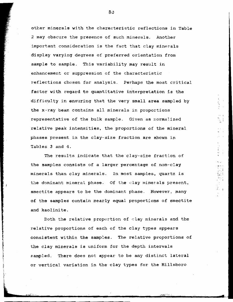
I I .
80
other minerals with the characteristic reflections in Table
2 may obscure the presence of such minerals. Another
important consideration is the fact that clay minerals
display varying degrees of preferred orientation from
sample to sample. This variability may result in
enhancement or suppression of the characteristic
reflections chosen for analysis. Perhaps the most critical
factor with regard to quantitative interpretation is the
difficulty in ensuring that the very small area sampled by
the x-ray beam contains all minerals in proportions
representative of the bulk sample. Given as normalized
relative peak intensities, the proportions of the mineral
phases present in the clay-size fraction are shown in
Tables 3 and 4.
The results indicate that the clay-size fraction of
the samples consists of a larger percentage of non-clay
minerals than clay minerals. In most samples, quartz is
the dominant mineral phase. Of the clay minerals present,
smectite appears to be the dominant phase. However, many
of the samples contain nearly equal proportions of smectite
and kaolinite.
Both the relative proportion of clay minerals and the
relative proportions of each of the clay types appears
consistent within the samples. The relative proportions of
the clay minerals is uniform for the depth intervals
sampled. There does not appear to be any distinct lateral
or vertical variation in the clay types for the Hillsboro
-,~· J' ,.,,-,_:
:1 • '

81
TABLE 3: Proportions of Phases Present in the Clay-size Fraction of Samples as Determined by XRD and Given as Normalized Relative Peak Intensities
Depth Smectite Musc./Ill. Kaol. Kao 1. Sample (ft) [001] [ 001] [ 001] [002]
HlB 6.5-7 60.00 26.00 HlC 17-22 38.32 10.08 19.75 17.69 HlD 30-32 --- 22.95 26.23 31.97
H3A 7-12 37.05 12. 61 20.18 17.06 H3B 17-22 47.12 27.61 23.33 14.54
H5A 2-3 43.18 34.10 --H5B 3-7 38.18 14.55 16.36 23.64 H5C @7 46.15 19.23 17.31 26.92 H5D 7.5-12 33.25 10.79 19.18 15. 54
H7A 2-6 25.41 13.99 11. 66 10.58 H7B 7-8 25.00 7.81 10.00 13.52 H7D 22-27 61.54 13 .11 25.00 26.75
H9A 2.5-5 10.46 -- 3.02 6.03 H9C 15-17.5 19.00 16.83 22.10 ----H9D 25-27.5 25.32 12.59 17.05 16.52
ii" HlOB 5-7.5 30.66 8.37 15.09 --. HlOC 10-12 46.81 29.79 31.91 HlOD 12.5-15 8.79 5. 41 5.68 HlOE 20-25 21.43 5.50 ----HllA @ll 7 52.09 19.67 22.87
-------·- ----~----------

82
TABLE 4: Nonclay Mineral Proportions Present in the Clay-size Fraction of Samples as Determined by XRD and Given as Normalized Relative Peak Intensities
~----Depth Quartz Quartz Calcite
Sample (ft. l [100] [101] [100]
HlB 6.5-7 - 78.00 100 HlC 17-22 22.68 96.85 100 HlD 30-32 36.06 100 47.54
H3A 7-12 16.47 82.05 100 H3B 17-22 20.94 100 66.19
H5A 2-3 --- 100 H5B 3-7 32.73 100 45.45 H5C @7 40.38 100 53.85 H5D 7.5-12 25.37 100 27.62
H7A 2-6 9.05 53.54 100 H7B 7-8 22.15 100 74.01 H7D 22-27 16.42 100 77.32
H9A 2.5-5 27.77 100 H9C 15-17.5 16.83 100 55.29 H9D 25-27.5 17.59 100 45.02
HlOB 5-7.5 14.45 60.35 100 HlOC 10-12 100 59.57 H10D 12.5-15 47.87 100 21.63 HlOE 20-25 2.78 37.35 19.21
HllA @17 16.00 100 66.81

83
landfill site. Figure 15 shows the relative distribution
of smectite, kaolinite, and muscovite/illite for each
sample.
Hydraulic conductivity estimates for sediment within
the saturated zone are presented in Table 5. The values
were derived from the results of field slug tests and from
textural analyses. The hydraulic conductivity values
ranged from 5.41 X 10⁻⁶ to 9.18 X 10⁻⁴ ft/s (1.65 X 10⁻⁶ to
2.80 X 10⁻⁴ m/s), with an average of 2.35 X 10⁻⁴ ft/s (7.18
X 10-5 m/s). The lower values correspond to silty clay
loam and the highest values to fine sand. Little
difference exists between cumulative grain-size
distribution curves of the samples (Appendix VII). Eight
of nine hydraulic conductivity values derived from those
curves are of the same order (3.28 X 10⁻⁵ ft/s (10-5 m/s))
and are representative of silt loam (Table 5). The
magnitude of the values estimated for the Hillsboro site
agree with those of Freeze and Cherry (1979, p. 29).
Values obtained from slug tests are in general agreement
with values obtained from textural analyses.
Apparent Resistivity
Apparent resistivity values for the Hillsboro landfill

1:/,
>'!ii'.,
•f:'I
Figure 15. Ternary plot of normalized relative peak intensities of smectite, kaolinite, and illite/muscovite from diffractograms of glycolated samples from the clay fraction of the Hillsboro sediment samples (see Table 3).

• •
SMECTITE
85
MUSC./ ILLITE
.. • ••
•
• • • . .. •
KAOLINITE
,,,t;;' .

86
·----~---------TABLE 5: Hydraulic Conductivity of the Hillsboro Landfill
Sediments ·----·
Piezometer Depth Description Hydraulic (ft) Conductivity (m/s)
--- ------------
Hl 30-32 Clayey silt 1. 65 X 10-6
Hl 2-4 Silty sand 4.95 X 10⁻⁵ *
H3 29.5-31.5 Sandy silt 1.12 X 10⁻⁵
HS 3-6 Silty sand 5.19 X 10⁻⁵ * HS 22-27 Sand l. 01 X 10-4 * H7 28-30 Sandy silt l. 02 X 10-5
H9 30-40 Silty sand 4.86 X 10⁻⁵ * H9 53.5-58.5 sand 1.33 X 10⁻⁴
H9 75-80 Sand 7.79 X 10⁻⁵ * HlO 23-25 Silty sand 2.80 X 10⁻⁴
HlO 20-25 Silty sand 7.79 X 10⁻⁵ *
Hll 11.5-17 Silty sand 6.10 X 10⁻⁵
Hll @17 Silty sand 4.95 X 10⁻⁵
Hl2 14.5-24.5 Sand 7.79 X 10⁻⁵
EW trench 16-18 Sand 7.08 X 10⁻⁵ *
sand lenses 4-7 Sand 6.14 X 10⁻⁵ *
----~-----------·---··----·
* Estimated from grain-size analyses, Appendix VI I.

87
are plotted vertically in Appendix VIII. From resistivity
theory it is important to remember that the resistivity
measurement is affected more, proportionately, by the
material at shallower depth. Accordingly, the logarithmic
plot gives greater emphasis to the readings at small
electrode spacings which correspond to material at shallow
depths (Soiltest, Inc., 1968). Although resistivity
boundaries do not necessarily correspond to stratigraphic
contacts, some of the lithologies and water table depths
can be correlated with the resistivity values of the log-log
profiles.
Very little contrast was evident in the observed field
data and high resistivity values were rare. Resistivity
values generally ranged from 30 to 600 ohm-ft (9.14 to
182.87 ohm-m), throughout the study area. The apparent
resistivity values are also presented in isoresistivity
maps for each of the electrode spacings used at the
Hillsboro site (Appendix IX}. The isoresistivity maps for
the electrode spacings (or depths) at or near the water
table indicate a "plume" of lower apparent resistivity
centered over the covered landfill trenches that extends
downgradient as three lobes to the southwest, south, and
southeast.
'' '

88
Fracture Analysis
The excavation of two trenches in the west-central
portion of the landfill.did not reveal an extensive network
of fractures, in fact, no measurable fractures were
observed and thus no qualitative results are presented
here. The trenches did, however, enable close observation
of the site stratigraphy. The upper 3 feet (0.9 m) of the
trenches consisted of light brown clayey silt. The
remainder of the exposed trench wall consisted of sandy
silt with inter-bedded, fine-grained sand lenses up to 6
inches (15 cm) wide and a couple of feet (0.6 m) long
(Figure 16). · Numerous rootlets were also observed (Figure
17). The rootlets were approximately 1/4 inch (0.6 cm) in
diameter and up to 3 feet (0.9 m) long. They were
generally highly oxidized and consisted of a hollow center
or a sand- or clay- filled center, and a dark outer organic
layer.
Precipitation at the Hillsboro Landfill
Precipitation at the Hillsboro landfill was estimated
between November of 1987 and August of 1988 by using
monthly totals from the U.S. Weather Bureau gauging station
at Hillsboro (Figures 18, 19, 20). During this time the
Hillsboro station recorded 8.65 inches (216 mm) of precip-
:::).-.: . .,,.

,,
,, ,.1:t.,, · .. it,_] )>!it
Figure 16. Fine-grained sand lenses exposed in excavated trench. Tape measure shown is in inches.

90

'i:ill ; ·rr!r.1
U'·_;t
::ti )liJ:
!)fl--~_. ' '
~ ·. ,1' \.,, ..... ,,;;1,,:''" ,;.,.i'
~;: ::'I; ;i ·1;,.
t': 1-:.:~-: 1,; ,·
':t·' ::;;-'.'. IF I t""
91
Figure 17. Rootlets observed in wall of excavated trench. Pocket knife shown for scale is approximately 2.5 inches (6.3 cm) long.

92

,f*f' ' l,1'-: lH
... :ii;, ,,. '
9J
Figure 18. Water-table levels and monthly precipitation totals for the Hillsboro landfill (piezorneters Hl, H3, HS, and HlS) .
l I
.,,

94
ft m 2
7 H!
C 8 <(
w :t: 9 ::!
3 H3 w 10 3: H15
3: II H5
0 ..J 12 w a)
13 4 :t: I- 14 a. w Cl 15
16 5
MARIAPR NOV DEC JAN FEB
1987

. ,:'' ' ~
'~1;1 ! ',
' ;'.'~;; : ;· /_)it
' :(;'1"1 '
; r.;:t: til,•::
r f 'l' 1::,; ·:, ~ ;:~- \" mi.
,,. I i:1 ,f;
·~'\ !~· q.,s.,
:s~: .,_· <"t'
,, ,I"''' ·,,_
Figure 19. Water-table levels and monthly precipitation totals for the Hillsboro landfill (piezometers H2, H4, H6, andHl4) .

ft m I
4
Cl <( 5 w :::: ...J 6 ...J 2 w 3: 7
3: 8 0 ...J 9 w a:i
:::: f- 11 0.. w 0 12
13
96
H2
. MAR APR MAY JUN
1987 1988
cm in. 6
5Z 0

,,
'I;
"' ' ' ;,1 -
,,
ft ' "' ~ :,." 1 . l•i.~ :r:;,'.'l•I
97
Figure 20. Water-table levels and monthly precipitation totals for the Hillsboro landfill (piezometer H7, H9, HlO, Hll, and H13).
I

98
ft. m 2
7
8 Cl
"' 9 UJ :c 3 ...J 10 ...J UJ 3 II 3: g 12 lLJ H7 a::J 13 4 :c I- 14 a. lLJ 0 15
16 i_5 ~::t:lilLl:..it=::::i::.:.l!.1.ti:.clUls.'.~~~:.1~,cf
JUL AUG· SEP
1987 1988

99
itation. The mean precipitation for this same period
(based on data from 1950-1980) is 16.30 inches (408 mm),
(Ruffner, 1985). Thus, precipitation at the Hillsboro
site was significantly below normal (47%),
Typically, 50 percent of the annual precipitation
recorded at the Hillsboro station occurs during the months
of May, June, and July (Ruffner, 1985). For 1988 this
totaled only 5.5 inches (137.5 mm), more than 4.5 inches
(112.5 mm) below normal. This three-month total was the
fourth lowest recorded during the last 38 years (National
Oceanic and Atmospheric Administration, 1988). In
addition, precipitation for the month of April was nearly
six times below normal. Essentially all of North Dakota
experienced drought conditions during the spring and summer
of 1988.
Recharge
A piezometer in which the screened interval inter
sects or is direcly below the water table, can be used to
determine potential groundwater recharge by monitoring
changes in the hydraulic head of the water table. At the
Hillsboro site seven of the piezometers either intersect
the water table or are screened within 3.3 feet (1.0 m)
below the water table. If the water table is within 9.8
feet (3.0 m) of the ground surface, the effects of
evapotranspiration and frost formation may contribute to

'
100
fluctuations of the water table, and the changes in
hydraulic head may not be indicative of actual groundwater
recharge (Rehm and others, 1982). Monthly water level
measurements at the Hillsboro site indicate that in the
northern part of the landfill, the maximum water table head
was less than 9.8 feet (3.0 m) below the ground surface.
Conversely, water level readings from piezometers in the
southern part of the landfill indicate the maximum water
table head to be greater than 9.8 feet (3.0 m) below the
ground surface. Therefore, the effects of evapotranspir
ation and frost there are negligible.
Figures 18, 19, and 20 indicate that the water table
fluctuations observed at the Hillsboro site were consistent
for each of the piezometers. Water levels measured in
piezometers H7, H9, HlO, Hll, Hl3, and Hl4 closely mirror
each other (Figures 19 and 20). Measured water levels in
piezometers H3 and HlS also indicate close correlation of
observed water levels (Figure 18). Water levels in
piezometers H4 and H6 display similar responses in that
each was dry or nearly dry from February through May, and
each reflects the increase in precipitation in May and June
(Figure 19). In general, most of the water levels
increased slightly from mid-February through late May with
a subsequent steady decline throughout the summer months of
June, July, and August. This reflects a water table rise
coincident with the spring thaw, and a water table decline
in response to prevailing drought conditions.

101
Recharge rates for the Hillsboro site were determined
from measured hydraulic heads. The hydraulic heads were
converted to vertical gradients between pairs of piezo
meters, which when multiplied by the measured hydraulic
conductivity, yields a downward flux of water in the
saturated zone (groundwater recharge rate) (Rehm and
others, 1982). The resulting vertical gradient at the
Hillsboro landfill averaged 1.36 X 10⁻¹ ft/ft (4.14 X 10⁻²
m/m). The corresponding average vertical flux rate, or
groundwater recharge rate is 2.55 X 10⁻⁶ ft/s (7.79 X 10⁻⁷
m/s).
Groundwater recharge was also calculated by multiply
ing the change in hydraulic head by the specific yield
(Rehm and others, 1982). A specific yield value of 0.08
(Johnson, 1967) was chosen as representative of the silt
loam beneath the Hillsboro site. Using this method, the
groundwater recharge rate averaged 2.0 X 10⁻⁹ ft/s (8.03 X
10-10 m/s).
The difference between these values is the result of
the uncertainty in the magnitude of the parameters used to
calculate the recharge rates. The greatest degree of
uncertainty is associated with the hydraulic conductivity
and the specific yield values used in the calculation. In
addition, neither of these methods takes into account the
effects of evapotranspiration and frost.
102
Application of HELP Model
The HELP modeling program provided a simple and rapid
means of simulating the amount of water movement through
the Hillsboro landfill. The results of program runs based
on mean monthly precipitation data and on monthly
precipitation totals recorded during the period of study
indicated that evapotranspiration losses were greater than
or equal to precipitation totals, and, thus, no percolation
occurred from the base of the landfill. Percolation was
not indicated by the model until record setting precipita
tion totals, as was the case in 1953, were used. Even then
evapotranspiration losses represented over 90 percent of
precipitation totals. A peak daily precipitation total of
nearly 4 inches (10 cm}, as on June 15, 1953, resulted in
the only measurable percolation through the landfill. The
results of the HELP modeling program suggest that leachate
generation from percolation occurs only during years of
above normal precipitation and, even then, only during
periods of intense rainfall, on the order of two to three
inches (5 to 7.5 cm) in a 24-hour period.
" " ;i
; : ''
'' " .! I 'I I
'' ''

DISCUSSION
Leachate ~orm~tion.and Characteristic~
The percolation of water through a landfill results in
a solution with high concentrations of both organic and
inorganic compounds, which is referred to as leachate. The
generation of leachate is accomplished through a number of
simultaneous biological, physical, and chemical changes,
including biological decay of organic compounds, chemical
oxidation of materials, gas evolution and diffusion, and
dissolution of organic and inorganic compounds (Chen and
Bowerman, 1974, p. 349). Perhaps the most important
factors affecting leachate formation are the types of waste
material, including organic-inorganic, degradable-nonde
gradable, and soluble-insoluble, and the landfill
conditions, including temperature, pH, moisture, and age.
Representative ranges for various inorganic constituents
in leachate from sanitary landfills are shown in Table 6.
The refuse for sanitary landfills comes primarily from
ordinary household and commercial solid waste. Typically,
paper comprises the largest share of sanitary landfill
refuse, approximately 37 percent (Environmental Protection
Agency, 1986b). Paper is usually quite low in moisture
content, however, and increased amounts of paper in refuse
have resulted in decreased rates of refuse breakdown (Chen
and Bowerman, 1974, p. 51). Conversely, food wastes
10J

104
TABLE 6: Concentration Ranges of Inorganic Leachate Constituents in Municipal Landfills.
Constituent
Alkalinity Cadmium Chloride Hardness Lead Nitrate pH Selenium Sulfate Total Dissolved Solids Turbidity Conductivity Copper Iron Magnesium Manganese Potassium Sodium Chromium Zinc
Concentration Range
0.1-20,350 mg/L 0-0.375 mg/L 30-5,000 mg/L 0.1-36,000 mg/L 0. 001-1. 44 mg/L
0.1-45 mg/L 3.5-8.5
0-2.7 mg/L 25-500 mg/L
725-55,000 mg/L 30-450
960-16,300 micromhos/cm 0.1-9 mg/L
200-5,500 mg/L 3-15,600 mg/L 0.6-41 mg/L 35-2,300 mg/L 20-7,600 mg/L 0.02-18 mg/L 0.6-220 mg/L
(after Environmental Protection Agency, 1986b, p. 4-12)

105
comprise approximately 8 percent of sanitary refuse and
may be extremely wet. In general, the moisture content of
mixed solid waste generated by a community ranges from 20
to 30 percent by weight (Weiss, 1974, p. 11). Moisture
content alone should not produce leachate.
Migration and Att"enuation"~LL~achate
The movement of landfill leachate in groundwater is
governed by the interaction of advection, dispersion, and
molecular diffusion. Advection refers to the transport of
contaminants at the same speed as the average linear velo-
city of groundwater. In most cases this is true of the
nonreactive solutes, generally the dissolved anions (Freeze
and Cherry, 1979, p. 75). Dispersion involves the spreading
of a volume of contaminants as it flows through the subsur
face. This spreading initiates mixing with uncontaminated
groundwater and ultimately results in dilution of the
contaminant plume. Dispersion may result in leachate
transport at velocities greater than the average ground
water velocity. Molecular diffusion is commonly included
as a component of microscopic dispersion (Anderson, 1984).
Molecular diffusion occurs as ions or molecules move from
"sites of higher to lower concentrations.
Leachate movement may be slowed or stopped by chemical
attenuation of inorganic contaminants involving adsorption,
precipitation, and oxidation or reduction. Foremost of

106
these controls is adsorption by clay minerals. Griffin and
others (1976) found that the attenuating ability of clays
was directly related to their cation exchange capacities.
They further noted that the most highly attenuated ions are
the trace metals.
Chemical Indicators of Contamination
Constituents most helpful in distinguishing ground
water contaminated by landfill leachate include specific
conductance, ammonium, chloride, bicarbonate, iron,
potassium, and sulfate (Saar and Braids, 1983). The
usefulness of these indicators generally reflects their low
susceptibility to attenuation and higher concentrations
within landfill leachate relative to natural occurrence.
Leachate Migration at the Hillsboro Landfill
Although contaminant levels appear to be low, the
chemical analyses (Appendix V) conducted on water samples
from the Hillsboro landfill suggest that degradation of the
groundwater beneath the landfill has occurred. The
isoconcentration maps (Appendix VI) reveal an increase in
ion concentrations over the background levels, most notably
the trace metals arsenic, cadmium, selenium, lead, copper,
chromium, iron, and manganese. The concentrations of these
trace metals ranged from 3.5 to 20 times above background
. ':,)."
107
levels. The isoconcentration maps indicate a contaminant
plume centered over the covered landfill trenches,
extending downgradient as lobes to the southwest, south,
and southeast. Reduced ion concentrations were observed
downgradient, away from the buried refuse. Major cations
such as potassium, sodium, magnesium, and calcium are
assumed to undergo concentration changes primarily due to
ion exchange. The trace metals may be limited in
occurrence due to solid phase solubility controls involving
sulfide, hydroxide, and carbonate (Cherry, 1983).
The configuration of the plumes on the isoconcentra
tion maps is believed to be the result of longitudinal and
transverse dispersion within the saturated zone. The shape
and position-of the plumes indicate that the buried refuse
is the source of contamination. However, it is apparent
that plume shape is not consistent for all the parameters.
The burial history of the refuse at the Hillsboro landfill
is not well documented. Thus, it is believed that the
plume shapes for some parameters reflect heterogeneities of
the refuse within the landfill trenches and isolated
disposal or surface spills outside of the covered trenches.
For example, arsenic appears in many pesticides. The
burial of empty pesticide containers in the northwest
corner of the landfill may have contributed to the
configuration of the arsenic plume. Isolated burial or
surface spills of lead acetate (accepted from the American
Crystal Sugar Company) may account for the lead plume. The

108
plume configuration for a number of parameters may have
been influenced by burn piles throughout the years.
Typically such burn piles contain large amounts of
construction debris, including gypsum wall board,
insulation materials, and roofing materials.
The higher levels of iron and manganese observed at
the Hillsboro site may have been derived from the sand
beneath the landfill; the redox conditions beneath
landfills can cause dissolution of oxide coatings of iron
and manganese on sand grains (Cherry, 1983). However, iron
may have come from stockpiling of iron which occurred on
site during the fall of 1987 and possibly in the past as
well. These two elements are apparently less influenced by
adsorption.
Factors perceived as contributing to the apparent low
levels of released contaminants include attenuation by
clays, low levels of precipitation, coupled with high
evapotranspiration losses, and the relatively short
residence time of the buried refuse. With regard to the
attenuation capabilities of the clays at the Hillsboro
landfill it should be reiterated that the clay-size
fraction of the samples is small (Appendix IV), and the
proportion of non-clay minerals within the clay-size
fraction is large (Table 4). However, Griffin and others
(1976) noted that sediment columns containing only two
percent smectite effectively attenuated landfill leachate
constituents, most notably the heavy metals. Griffin and

109
others (1976) attributed the attenuating ability of clays
to their cation exchange capacities. Of special importance
in smectite is the sodium-calcium exchange reaction (Freeze
and Cherry, 1979, p. 133). Replacement of calcium by
sodium results in expansion of the smectite clay structure
which can effectively decrease permeability. It is
expected that clay adsorption and ion exchange within the
clayey silt and sandy silt intervals, which contain at least
10 percent clay-size sediment, are important mechanisms
limiting the mobility of contaminants.
The effects of evapotranspiration were surely more
pronounced in light of the drought conditions experienced
during the period of study. Measured evapotranspiration in
North Dakota·is on the order of 1.5 times greater than
precipitation (Rehm and others, 1982, p.18), a scenario
substantiated by the HELP computer model. In spite of
this, recharge can occur, dependent on the intensity and
duration of precipitation. Significant recharge in the
summer months likely occurs only when very high intensity
rains result in high enough infiltration rates for the
water to quickly pass through the root zone. During the
summer of 1988, such recharge events were virtually
nonexistent. The lack of infiltration and subsequent
recharge suggests that very little if any leachate should
reach the water table at the Hillsboro site. However,
because the depth to the water table is between 5.4 and 11
feet (1.66 and 3.37 m) below the surface in the northern

110
part of the landfill, burial of refuse in trenches 15-feet
{4.57 m) deep ensure that the lower portion of the land
fill would become saturated. It is expected that the
trenches were designed with a slight northward slope, and
as such, these saturated conditions within the refuse were
more prevalent in the northern part of the landfill. Thus,
even without infiltration through the landfill cover,
leachate would be expected to be produced through lateral
migration of groundwater into the refuse-filled trenches.
Another factor influencing the production of leachate
is time. The Hillsboro landfill was in operation less than
12 years. Given the likelihood that the buried refuse
consists of large amounts of paper and that large portions
of the landfill have remained relatively dry, it appears as
though 12 years should not be considered an unusually long
period of time with regard to leachate generation. In
fact, given the calculated average linear velocity of 8.59
X 10-7 ft/s {2.62 X 10⁻⁷ m/s), groundwater travel time from
piezometer Hl to Hl4 is nearly 28 years. Similar invest
igations in other landfills throughout North Dakota suggest
that it is not uncommon to find newspaper that has been
buried in excess of ten years and yet displays little
evidence of breakdown {Tillotson, 1988). At the Hillsboro
landfill, a shallow test hole in the oldest portion of the
site revealed much the same (Figure 21). Steiner and
others {1971} note that leachate appearance may be offset
from the initial time of emplacement by as much as 20

r
·~J:: ':;;. ;~;; '.:; 11iiH 1
i•1!fl t
"' ~~V) . . :r'. "~
111
Figure 21. Newspaper recovered from a shallow test hole in the oldest portion of the landfill site.


113
years, and that short-term studies may be inadequate to
establish the magnitude of the problem.
In addition to the preceding discussion, a number of
variables, including placement of the piezometers, depths of
screened intervals, and the parameters tested for, may
account for the apparent low levels of contaminants. The
parameters tested for did reveal a pattern; however, several
other parameters useful in leachate plume delineation,
including ammonium, boron, mercury, and freon were not
analyzed for. Also, organic analyses, including total
organic carbon (TOC) may have revealed more extensive
groundwater contamination beneath the Hillsboro site.
Two possible alternatives of contaminant movement at
the Hillsboro landfill are presented in Figure 22. In the
first case, low levels of contaminants within the leachate
plume are detected downgradient of the buried refuse
(Figure 22B). In the second case (Figure 22C), due to the
relatively high vertical gradient beneath the landfill
site, the leachate plume moves primarily downward and
remains directly under the contamination source, and
subsequent movement with the groundwater flow allows the
main body of the plume to pass undetected below the
monitoring equipment. However, it appears unlikely that
such plume movement would not be detected by piezometer H9.
The possible existence of a deep plume was the reason for
attempting to install piezometer H9 at a depth of 82 feet
( 25 m) •

: I,.
I I, t 1·•_ ; j':_ ! 1-.· ..
!, : : ..
r.1: l ~-·! ' ~.
U:i ·;
::;;:;.: \!!•h"i' ~) ·I·., -'11,r,,
•• ri·,,. I itt" n-,.,.., '· ;kit_ :, ~J, !I'·: . I ~J;)II'-' !.11,
114
Figure 22. Two alternative contaminant plume configurations beneath the Hillsboro landfill. (A) North-south cross-section at the landfill displaying the location of piezometers, the position of the water table, and the geology beneath the site. (B) Low levels of contaminants are detected downgradient of the buried refuse and/or (CJ, because of a relatively high vertical gradient, the leachate plume moves primarily downward and remains directly under the contamination source. For lithologic symbols see Figure 13.
l ' I I
I

ft. 0
10
20
30
40
50
60
115
A
8
C
L
-:--------
II BASE OF I" AQUIFER --- -
m
0
5
10
15
20
!'
11:
: 'I.
':,, 'ljl
l!i· , II i,
'<' 11,'
I ii' ., .
•Ii
'I

116
Apparent Resistiyiq
Quantification of surface resistivity results for
comparison with the results of water sampling was attempted
for the Hillsboro site. If the apparent resistivity values
reflect the quality of groundwater, then isoresistivity
contours (Appendix IX) should parallel isoconcentration
contours (Appendix VI) (Klefstad and others, 1975).
The contours of the isoconcentration maps for
potassium and chloride roughly paral.lel the isoresistivity
maps for the 8-, 10-, 12-, and 16-foot (2.4-, 3.1-, 3.7-,
and 4.9-metre) electrode spacings. The contours of the TDS
and bicarbonate isoconcentration maps correlate to a lesser
degree with the isoresistivity maps. The high TDS
concentrations in H2 and Hll do not appear to be reflected
in the field data. In general, the change in resistivity
sought as an indicator of contamination was small and
essentially undetectable. A slight reduction in
resistivity values centered over the covered trenches may
be attributed to the lack of vegetative cover at the time
of the survey (Murphy and Kehew, 1984).
With regard to correlation between apparent
resistivity and lithology, perhaps the best results were
obtained at resistivity station 3 {Appendix VIII). The
presumably low moisture content of the near-surface sandy
silt account for the highest resistivity values. The

117
influence of a clayey layer at approximately 24 feet {7.3
m) is reflected in the lowest resistivity values, whereas
the cleaner sand at depth again produces higher values. In
general, the log-log plots of apparent resistivity versus
electrode spacing reflect the higher near-surface values of
dry sand and sandy silt, the lower uniform values of
saturated sandy silt, the lowest values of clayey layers,
and the higher values .of a clean sand at depth. In some
cases, the high silt content and the low degree of
consolidation of these deposits may have attributed to the
poor definition of layer boundaries (Murphy and Kehew,
1984).
Interpreted Resistivity
The apparent resistivity values obtained reflect the
true resistivity of the geologic sediments only if they are
homogeneous and isotropic (Yazicigil and Sendlein, 1982).
As this is rarely the case in the subsurface, a computer
program developed by Zohdy and Bisdorf {1988} was used to
interpret the apparent resistivity values and automatically
calculate layer thicknesses and resistivities (Appendix
VIII). Profiles of interpreted resistivity values for the
Hillsboro site are in general agreement with the log-log
plots of apparent resistivity versus electrode spacing.
The position of the water table appears to be accurately
represented by the interpreted profiles.

118
A major shortcoming of the computer program rests in
modifications made to the PC version to enable the
interpretation of Wenner sounding data. These modifica
tions may have introduced as much as 10 percent error into
the data interpretation (Bisdorf. 1988). In addition,
Kehew and Groenewold (1983) have pointed out that at the
larger electrode spacings, very small changes in potential
difference result in significant differences in apparent
resistivity. Yet the sensitivity of the computer program
is such that small changes in the slope of the apparent
resistivity curve can profoundly alter the interpreted
layering sequence. Thus, in sediments with a high degree
of electrical uniformity, correlation between sediment
boundaries and the computer-generated sequence of layers is
difficult.
!,im.i ta tions in .Earth ~eEi.!stiyJ...:tY_~Surveying
Successful application of resistivity methods to
groundwater contamination investigations depends on
favorable conditions, including uniform subsurface
conditions, a shallow groundwater table, and a significant
conductivity contrast between contaminated and natural
groundwater (Klefstad and others, 1975). If these
conditions are not met, they impose significant limitations
which can preclude the success of the resistivity survey.
A number of conditions favorable to resistivity

119
surveying exist at the ·Hillsboro landfill, including a
shallow groundwater table and relatively uniform subsurface
conditions. However, very little contrast was evident in
the observed field data. The interpretation and correla
tion of resistivity data are more accurate when orders of
magnitude contrasts occur (Kehew and Groenewold, 1983).

CONCLUSIONS
The Hillsboro landfill is representative of a landfill
that was located, operated, and designed with little or no
consideration of the geologic and hydrogeologic conditions
of the site. Its location above a major aquifer, within
permeable surface materials, and within shallow water table
conditions should not have been permitted. Operation as an
open dump and acceptance of lead acetate from the American
Crystal Sugar Company, coupled with the fact that the land
fill cells are unlined and at least portions of the buried
refuse are below the water table, has undoubtedly increased
the potential for groundwater contamination beneath this
site.
Although the water sampling activities conducted as
part of this project were limited by financial and time
constraints, as well as by drought conditions, the results
of this study do, indeed, reveal that groundwater degrada
tion beneath the buried refuse has occurred. In addition,
the following can be concluded:
1. The depth to the water table varied from 5.4 to 11 feet
(1.7 to 3.4 rn) below the surface in the northern part of
the landfill and from 10.6 to 13.2 feet {3.2 to 4.0 m)
below the surface in the southern part of the landfill
site.
120

121
2. Water table maps indicate that groundwater beneath the
site is flowing to the south-southeast, away from covered
landfill trenches.
3. The silty clay loam, silty loam, silt, and sand, which
define the stratigraphy of the Hillsboro landfill, are
characteristic of deposition in proglacial lakes and the
fluvial influence of drainage into these shallow lakes.
4. Smectite is the dominant clay mineral present in the
Hillsboro sediments.
5. The amount of leachate generated at the Hillsboro
landfill is small because of, a) normally low amounts of
infiltration, b) absorption of water by large amounts of
paper within the compacted buried refuse, c) comparatively
little decay as a result of the relatively short residence
time of the buried refuse, d) attenuation by smectite
clays, and e) dilution by mixing with uncon-tam.inated
groundwater.
6. Although well below maximum permissible concentrations,
the concentrations of the trace metals arsenic, cadmium,
selenium, lead, copper, chromium, iron, and manganese
ranged from 3.5 to 20 times more than background levels.
7. Quantification of electrical earth resistivity results

122
(for comparison with the results of water sampling) proved
difficult due to the low concentration of contaminants and
the associated negligible contrast between the conductivi
ties of contaminated and natural groundwater.
8. In spite of the low levels of contaminants detected,
the position of the shallow water table wi.thin the lower
portions of the refuse-filled trenches poses a significant
threat to groundwater beneath the landfill.

RECOMMENDATIONS
Implicit in the description of the Hillsboro landfill
is the recommendation to avoid such locations for waste
disposal. The inadequacies of the site and the potential
for groundwater contamination beneath the site ultimately
resulted in the closure of the landfill and the initiation
of this study. Thus, given the potential for groundwater
contamination as suggested by the setting of the landfill
and by the results of this study, groundwater monitoring
should continue at this site. Also, given the limitations
imposed on water sampling by drought conditions, such
monitoring should include a wet spring during which normal
recharge occurs and optimum leachate production and
movement might be expected.
Although high levels of contaminants were not
detected, it is expected that organic sampling may provide
useful indicaters of leachate production. Additional
water sampling, including organic analysis, is appropriate.
The cation exchange capacities of the Hillsboro
sediments should be determined. This is important in light
of the fact that the attenuating ability of clays is a
function of their cation exchange capacities.
Concern over the proximity of the landfill to the
Hillsboro aquifer warrants more accurate definition of the
aquifer boundaries beneath the site. Accordingly, several
deep ( 50 to 100 feet ( 15. 2 t.o 30. 5 m) ) test holes should be
123
I I
ii
., I I

124
drilled. Such drilling should include the installation of
at least one deep piezometer (> 80 ft (24.4 m)) in order to
better evaluate the characteristics of groundwater within
the aquifer.
The placement of additional piezometers within the
present monitoring scheme should also be considered.
Installation of a piezometer nest near Hl2 (Figure 7),
including the addition of both a shallower and deeper
piezometer, would permit better interpretation of background
conditions. Other possible additions might include
piezometer nests incorporating the downgradient wells H13,
Hl4, and HlS (Figure 7). Due to the shallow water table at
the site, instrumentation of the vadose zone is probably
unnecessary. The incorporation of these suggestions would
serve to strengthen aspects of this study which were limit
ed by financial and time constraints, and by drought condi
tions.
~"' ', '' _______ .............................. .__--"""~~-··=····="·"'-"-' '"""" ~' ' '
,;
" ,,
,, 'I ,, ,,
·, ,, 1:

APPENDICES
'
'I
ii:
ll i 11' :r " 1, ,,
ii:,
I!'
. I
,JI j' i
' I ' ·: I "

126
APPENDIX I
Piezometer Elevations and Screened Intervals
:1
d
·' I 111 ., '

127
Piezometer Surface Elevation Screened Interval ( ft) (ft below the surface)
Hl 930 30-32
H.2 930 12
H3 931 29.5-31.5
H4 931 7.5-12.5
HS 932 28-30
H6 932 7-12
H7 935 28-30
HS 935 7-12
H9 932 53.5-58.5
HlO 932 23-25
Hll 932 11.5-17
Hl2 933 14.5-24.5
Hl3 932 11.9-21.9
Hl4 931 8-18 'I ,,
Hl5 930 7.5-17.5
128
APPENDIX II
Lithologic Description of Drill Holes

Hl
Depth (ft)
0-2
2-4
4-17
17-22
22-27
27-30
30-32
129
Description
Fill
Sand, dark grayish brown (lOYR,4/2), color wet=very dark grayish brown (lOYR, 3/2), finemedium grained, moderately sorted, subangular-subrounded(0.5) sphericity(0.7).
Sand and silt, light yellowish brown (lOYR, 6/4), color wet= brown (lOYR, 4/3), fine-medium grained, subangular-subrounded, some angular grains {0.3), sphericity {0.5-0.7), FeO stain on sand grains.
Sand and silt, very pale brown (lOYR, 7/4), color wet=dark yellowish brown (lOYR, 4/4), fine-grained, subrounded (0.5), well sorted, sphericity (0.3).
Sand and silt, light yellowish brown (lOYR, 6/4), color wet= brown (lOYR, 4/3), fine-grained, well-sorted, angular-subrounded (0.3), sphericity (0.5).
Sand and silt, light brownish gray (lOYR, 6/2), color wet=grayish brown (lOYR, 5/2), finemedium grained, well sorted, subangular-subrounded (0.5), sphericity (0.7).
Sand, silt, and some clay, gray (lOYR, 6/1), color wet=dark gray (lOYR, 4/1), v. fine-fine grained, well sorted.
I
' ' I, 'I '
'.I
:r 'I "
·- - . ;, ,, . \. ;,-:.-·~-,,·.tr:-.·

H2
Depth {ft)
H3
0-2
2-4
4-12
Depth (ft)
0-2
2-5
5-7
7-9
9-22
,' -,,.\ ·"0';·.
1.30
Description ----···--
Fill
Sand, dark grayish brown {lOYR,4/2), color wet=very dark grayish brown (lOYR, 3/2), finemedium grained, moderately sorted, subangular-subrounded(0.5) sphericity(0.7).
Sand and silt, light yellowish brown (lOYR, 6/4), color wet= brown (lOYR, 4/3), fine-medium grained, subangular-subrounded, some angular grains (0.3), sphericity (0.5-0.7), FeO stain on sand grains.
Description
Topsoil
Sand and silt, medium brown, fine to medium grained.
Sand and silt, light yellow brown, fine-medium grained.
Sand and silt, alternating red (2.SYR, 5/6) and gray (lOYR, 6/1) layers, very fine-grained, well sorted, subrounded.
Sand and silt, light yellowish brown (lOYR, 4/6), color wet= dark yellowish brown (lOYR, 4/6), v. fine-fine grained, well

22-32
H4
Depth (ft)
ES
0-2
2-5
5-7
7-9
9-12.5
Depth (ft}
0-1
1-3
131
sorted, subrounded, sphericity (0.7).
Sand and silt, pale brown (lOYR, 6/3), color wet=dark grayish brown (lOYR, 4/2), similar to above.
Description
Topsoil
Sand and silt, medium brown, fine to medium grained.
Sand and silt, light yellow brown, fine-medium grained.
Sand and silt, alternating red (2.5YR, 5/6) and gray (lOYR, 6/1) layers, very fine-grained, well sorted; subrounded.
Sand and silt, light yellowish brown (lOYR, 4/6), color wet= dark yellowish brown (lOYR, 4/6), v. fine-fine grained, well sorted, subrounded, sphericity (0. 7).
Description
Topsoil
Sand, brown (lOYR, 5/3), color wet=dark brown {lOYR, 3/3), finemedium grained, moderately sorted, subangular (0.3), sphericity (0.9).

3-6
6-7.5
7.5-12
12-22
22-32
H6
Depth (ft)
0-1
1-3
3-6
lJ2
Sand and silt, very pale brown {lOYR, 7/3), color wet=dark yellowish brown (lOYR, 4/4), very fine-fine grained, well sorted, subrounded (0.5), sphericity {0.7), FeO stained.
Clay and silt, very pale brown (lOYR, 7/3), and yellowish red (5YR, 5/8), color wet=yellowish brown {lOYR, 5/4) and dark yellowish brown (lOYR, 4/4), FeO stained.
Sand and silt, light yellowish brown (lOYR, 6/4), color wet=dark yellowish brown (lOYR, 4/4), very fine grained, moderately sorted, subangular ( 0. 3), spherici ty _(O. 9).
Sand, some silt, pale brown (lOYR, 6/3), color wet=dark brown (lOYR, 3/3), medium-coarse grained, well sorted, subangular to subrounded (0.5), sphericity (0.7-0.9).
Sand, pale brown (lOYR, 6/3), color wet=dark brown (lOYR, 3/3), fine to medium grained, very well sorted, subrounded to rounded (0.5), sphericity (0.9).
Description
Topsoil
Sand, brown (lOYR, 5/3), color wet=dark brown (lOYR, 3/3), finemedium grained, moderately sorted, subangular (0.3), sphericity (0.9).
Sand and silt, very pale brown (lOYR, 7/3), color wet=dark yellowish brown (lOYR, 4/4), very fine-fine grained, well sorted,
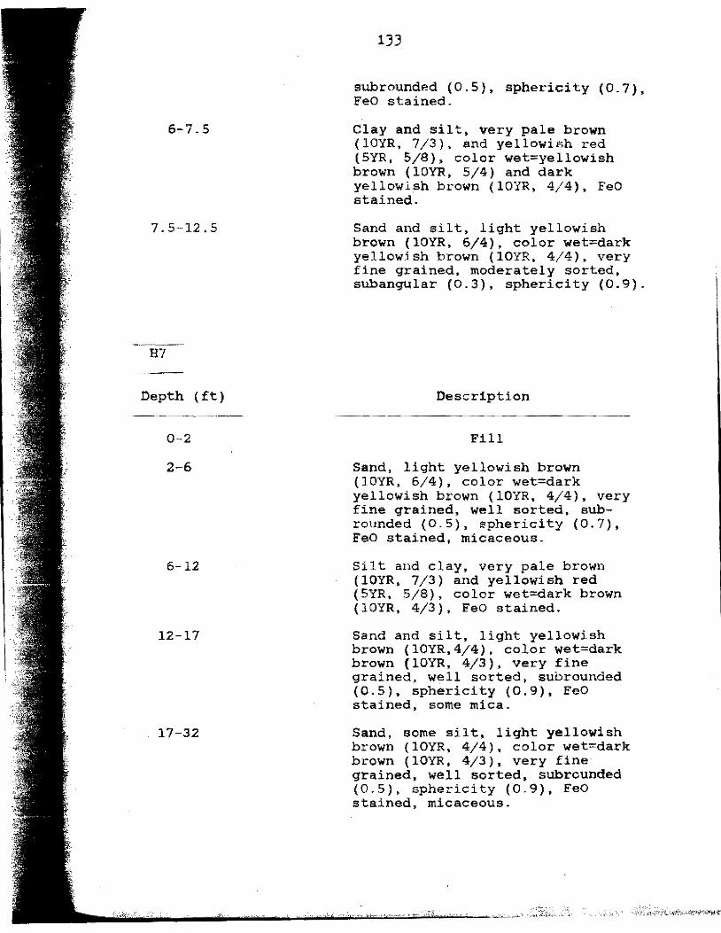
6-7.5
7 .5-12 .5
Depth (ft)
0-2
2-6
6-12
12-17
17-32
lJJ
subrounded (0.5), sphericity (0.7), FeO stained.
Clay and silt, very pale brown (lOYR, 7/3), and yellowish red (5YR, 5/8), color wet=yellowish brown (lOYR, 5/4) and dark yellowish brown (lOYR, 4/4), FeO stained.
Sand and silt, light yellowish brown (lOYR, 6/4), color wet=dark yellowish brown (lOYR, 4/4), very fine grained, moderately sorted, subangular (0.3), sphericity (0.9).
Description
Fill
Sand, light yellowish brown (lOYR, 6/4), color wet=dark yellowish brown (lOYR, 4/4), very fine grained, well sorted, subrounded (0.5), sphericity (0.7), FeO stained, micaceous.
Silt and clay, very pale brown (lOYR, 7/3) and yellowish red (SYR, 5/8), color wet=dark brown (lOYR, 4/3), FeO stained.
Sand and silt, light yellowish brown (lOYR,4/4), color wet=dark brown (lOYR, 4/3), very fine grained, well sorted, subrounded (0.5), sphericity (0.9), FeO stained, some mica.
Sand, some silt, light yellowish brown (lOYR, 4/4), color wet=dark brown (lOYR, 4/3), very fine grained, well sorted, subrounded (0.5), sphericity (0.9), FeO stained, micaceous.
,',. :" \.

HS
Depth (ft)
H9
0-2
2-6
6-12
Depth (ft)
0-2
2-5
5-7.5
7.5-15
134
Description
Fill
Sand, light yellowish brown (lOYR, 6/4), color wet=dark yellowish brown (lOYR, 4/4), very fine grained, well sorted, subrounded (0.5), sphericity (0.7), FeO stained, micaceous.
Silt and clay, very pale brown (lOYR, 7/3) and yellowish red (5YR, 5/8), color wet=dark brown (lOYR, 4/3), FeO stained.
Description
Fill
Sand and silt, very pale brown (lOYR, 7/3), color wet=yellowish brown (lOYR,5/4), fine grained, well sorted, subangular to subrounded (0.5), sphericity (0.7), some FeO staining.
Sand, pale brown (lOYR, 6/3), thinly laminated, color wet= dark yellowish brown (lOYR, 4/4}, fine-grained, well sorted, subangular to subrounded (0.5}, sphericity (0.7).
Sand and silt, light gray (lOYR, 7/1} and light yellowish brown (lOYR, 6/4), color wet=grayish brown (lOYR, 5/2} and yellowish brown (lOYR, 5/6), very fine grained, well sorted, subrounded, FeO stained, thinly laminated in
1------------------·''ii.i'.''\ii.i~-",i,."'''ioioii ___ .,. ________ ..... ___ ..._ ..... _ '"

HlO
15-24
24-25
25-30
30-40
40-82.5
Depth (ft)
0-2
2-2.5
2.5-5
5-12.5
135
lower 5 feet.
Sand and silt, pale brown (lOYR, 6/3), color wet=dark brown (lOYR, 4/3), very fine to fine grained, well sorted, subrounded (0.5), sphericity (0.7).
Clay and silt, gray.
Sand and silt, pale brown (lOYR, 6/3), color wet=dark grayish brown (lOYR, 4/2), very fine grained, micaceous.
Sand, light brownish gray (lOYR, 6/2), color wet=grayish brown (lOYR, 5/2), medium grained, subangular to subrounded (0.3-0.5), sphericity (0.9), moderately sorted.
Sand, gray (lOYR, 6/1), color wet=gray (lOYR, 4/1), salt and pepper, medium to coarse grained, moderately sorted, subangular to rounded (0.3-0.7), sphericity (0.7-0.9), some FeO stain, sand coarsens downward.
Description
Fill/Topsoil
Clay, light gray (lOYR, 7/1), color wet=brown (lOYR, 4/3).
Sand, light yellowish brown (lOYR, 6/4), color wet=yellowish brown (lOYR, 5/4), very fine grained, well sorted, subangular (0.3), sphericity (0.7), FeO stained, some mica flakes.
Sand, pale brown (lOYR, 6/3), color wet=yellowish brown (lOYR, 5/4), fine grained, moderately

12.5-17
17-17.5
17.5-25
Hll
Depth (ft)
0-2
2-2.5
2.5-5
5-12.5
12 .5-17
136
sorted, subangular-subrounded (0.3-.5), sphericity (0.7), thinly laminated, FeO stained lamina prominant, micaceous.
Sand, pale brown (lOYR, 6/3), color wet=dark brown (lOYR, 4/3), laminae absent, fine-medium grained, subrounded-well rounded (0.7), moderately sorted, sphericity (0.7-0.9).
Clay and silt, very pale brown (lOYR, 7/4), coloR wet=yellowish brown ( lOYR, 5/4).
Sand and silt, pale brown (lOYR, 6/3), color wet=dark brown (lOYR. 3/3), medium grained, moderately sorted, subrounded to rounded (0.7), sphericity (0.9).
Description
-·--··-·-·-·--·· --------
Fill/Topsoil
Clay, light gray (lOYR, 7/1), color wet=brown (lOYR, 4/3).
Sand, light yellowish brown (lOYR, 6/4), color wet=yellowish brown (lOYR, 5/4), very fine grained, well sorted, subangular (0.3), sphericity (0.7), E'eO stained, some mica flakes.
Sand, pale brown (lOYR, 6/3), color wet=yellowish brown (lOYR, 5/4), fine grained, moderately sorted, subangular-subrounded (0.3-0.5), sphericity (0.7), thinly laminated, FeO stained lamina prominant, micaceous.
Sand, some silt, light yellowish brown (lOYR, 6/4), color wet= dark yellowish brown (lOYR, 3/4),

137
very fine to fine-grained, well sorted, subrounded to rounded (0.7), sphericity (0.9), FeO stained.
I
I .
I
··"'····
138
APPENDIX III
Water Table Maps
·1: 1:
I

::,.,.1: ,, • I,, , •. 1 1.1:
; :;:: -~I,:/
•·' 1· l,
r · l
' 11,::,:l 1 ··
¥" I I -H
~);;::: •\j, 1· 17- I ,1
V>-1 i :~!
~:·; ; l ·:!
\,111!:
Arrows indicate the direction of groundwater £low.

A
B
C
Pl EZOMETERS
SURFACE TOPOGRAPHY
WATER TABLE NOV. 1987
C.I. a LO ft 0.304 m
140
,, ii II II
11 ---- 920 0
"
0 IOOm ---=== 0 500ft
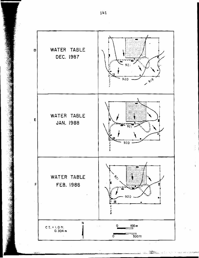
D
E
F
WATER TABLE
DEC. 1987
WATER TABLE
JAN. 1988
WATER TABLE
FEB. 1988
C.L • 1.0 It. 0.304m
141
I ,, Bl t JI •
o.,..-==':::ioo m
0 500ft

WATER TABLE
G MAR. 1988
H
- NO WATER LE'IE:..S TAKEN-
WATER TABLE APR. 1988
WATER TABLE MAY 1988
C.I. 0 I.Oft. 0.304m
142
0
0 100m --=== 500ft
'l',,;, k', ,_

WATER TABLE JUN. 1988
WATER TABLE JUL. 1988
WATER TABLE AUG. 1988
C.I. : 1.0 ft. 0.304 m
14J
~ " ,,
0
., • !
920 --~·
0 100m --=== 500ft

144
APPENDIX IV
Textural Analyses
•
" r I

145
·-·--~ Sample Depth(ft) Description % Sand % Silt % Clay ~·~-·-· . ---
Hl 2-4 Silty sand 50 39 11 Hl 6.5 Sandy silt 30 61 9 Hl 7-12 Sandy silt 40 57 3 Hl 17-22 Sandy silt 25 73 2 Hl 22-27 Sandy silt 24 73 3 Hl 27-32 Sandy silt 17 79 4 Hl 30-32 Clayey silt 3 62 35
H3 7-12 Silt 3 89 8 H3 12-17 Silt 9 87 4 H3 17-22 Sandy silt 19 78 3 H3 22-27 Sandy silt 19 79 2 H3 27-32 Sandy silt 18 80 2
HS 2-3 Silty sand 72 21 7 HS 3-6 Silty sand 53 41 6 HS 6-7 Clayey silt 17 55 28 HS 7.5-12 Sandy silt 35 58 7 HS 12-17 Silty sand 79 14 7 HS 17-22 Sand 92 8 0 HS 22-27 Sand 92 8 0
H7 2-6 Sandy silt 32 65 3 H7 7-8 Clayey silt 2 88 10 H7 12-17 Sandy silt 16 77 7 H7 17-22 Sandy silt 21 75 4 H7 22-27 Sandy silt 39 59 2 H7 27-32 Sandy silt 37 61 2
., ;

146
Sample Depth(ft) Description % Sand % Silt % Clay ---·-----··
H9 0-1 Fill 29 62 9 H9 2-5 Sandy silt 34 55 11 H9 5-7.5 Sandy silt 27 69 4 H9 7.5-9 Sandy silt 14 82 4 H9 9-10 Sandy silt 16 80 4 H9 10-12.5 Silt 1 94 5 H9 12.5-13.5 Silt 2 90 8 H9 13.5-15 Sandy silt 12 79 9 H9 15-16 Sandy silt 10 83 7 H9 16-17.5 Sandy silt 29 67 4 H9 22.5-23.5 Sandy silt 25 71 4 H9 23.5-25 Sandy silt 18 78 4 H9 25-27.5 Silt 4 91 5 H9 30-40 Silty sand 77 23 0 H9 40-50 Silty sand 88 12 0 H9 55-60 Sand 90 8 2 H9 65-70 Sand 90 7 3 H9 70-75 Sand 91 7 2 H9 75-BO Sand 91 7 2
HlO 0-2 Fill 38 46 14 HlO 2-5 Silt 5 88 7 HlO 5-7.5 Sandy silt 28 69 3 HlO 7.5-8 Silt 6 93 l HlO 8-10 Silt 8 88 4 HlO 10-11 Sandy silt 48 51 1 HlO 11-12 Sandy silt 47 51 2 HlO 12-13 Sandy silt 44 47 9 HlO 13-15 Silty sand 77 23 0 HlO 15-16 Sand 92 s 0 HlO 16-17 ·clayey silt 4 86 10 HlO 20-25 Silty sand 83 14 3
Hll @17 Silty sand 53 42 5
,, ~ .. ~

,,
147
APPENDIX V
Water Analyses
l _____ ... .;.. _____________ .... _______________ _..::t:.;·,,.,,:,,;,;:;;.:·, .. · _____ ,.. _____ _
'C'C'

~ i 111, ' ' 1'.: 11.
" '· 1,
,'l: :,l• rl,'., •II'
Total A As HC03 Cd C03 Cl F Total H Pb N03 pH Temp. Se % Na S04 TDS Turb. SAR Cond. Ba Ca Cu Fe Mg Mn K Na Cr Zn
148
Total alkalinity (CaC03) in milligrams/litre Arsenic in micrograms/litre Bicarbonate in milligrams/litre Cadmium in micrograms/litre Carbonate in milligrams/litre Chloride in milligrams/litre Fluoride in milligrams/litre Total hardness in milligrams/litre Lead in micrograms/litre Nitrate reported as Nin milligrams/litre Field pH Field temperature in degrees Celsius Selenium in micrograms/litre Percent sodium Sulfate in milligrams/litre Total Dissolved Solids in milligrams/litre Turbidity Sodium absorption ratio Specific conductance in micromhos/cm Barium in micrograms/litre Calcium in milligrams/litre Copper in micrograms/litre Iron in milligrams/litre Magnesium in milligrams/litre
.Manganese in milligrams/litre Potassium in milligrams/litre Sodium in milligrams/litre Chromium in micrograms/litre Zinc in micrograms/litre

149
Piezometer
Hl H2 H3 H4 HS
Total A 185 646 291 390 272 As 3.1 1.1 1.9 1.2 5.8 HC03 226 789 355 476 332 Cd 2.26 2.11 0.78 0.66 1.51 C03 Cl 2.1 10.7 2.3 2.2 3.6 F 0.2 0.1 0.2 0.8 0.3 Total H 212 704 292 430 273 Pb 1.3 1. 6 5.1 0.7 0.1 N03 5.0 1.2 0.1 pH 7.75 7.15 7.79 7.75 7.75 Temp. 7 7 6 7 7 Se 1.0 1.0 % Na 2.1 1.8 3.2 3.8 5.6 S04 23 24 9.0 42 9.0 TDS 214 682 289 423 276 Turb. 2.0 3.0 < 1 2.0 2.0 SAR 0.06 0.10 0.11 0.17 0.20 Cond. 351 1023 463 647 459 Ba 317 138 227 112 177 Ca 55 146 64.8 63.2 57.1 Cu 4.7 4.7 6.1 0.7 2.4 Fe 0.136 0.215 0.033 0.387 0.009 Mg 18.1 82.5 31. 5 66.1 31. 7 Mn 0.422 0.359 0.475 0.021 0. 728 K 1.90 2.10 2.50 1.60 2.80 Na 2.10 6.10 4.50 7.90 7.50 Cr 12. 7 1.90 4.50 Zn 53 138 70 154 80

150
' Piezometer
H6 H7 HS H9 HlO
Total A 530 292 X 287 245 As 1.1 1.4 X 3.9 1.3 HC03 647 356 X 350 299 Cd 1.0 1.0 X 1.24 0.41 C03 X Cl 6.8 1. 7 X 18.0 5.3 F 0.1 0.3 X 0.2 0.2 Total H 554 291 X 325 307 Pb 0.9 0.5 X 0.7 0.6 N03 0.2 0.2 X 10.2 pH 7.61 7.78 X 7.75 7.71 Temp. 8 X 8 8 Se 1.0 X 4.0 % Na 1.7 2.8 X 4.5 2.9 S04 16 10 X 33 30 TDS 537 287 X 343 334 Turb. 2.0 < 1 X 5.0 2.0 SAR 0.08 0.10 X 0.17 0.11 Cond. 829 461 X 527 487 Ba 158 229 X 239 256 Ca 136 56.7 X 76.5 64.0 Cu 5.2 5.2 X 1.4 2.2 Fe 0.240 0.047 X 0.685 0.254 Mg 52 36.2 X 32.6 35.7 Mn 0.124 0.828 X 0. 527 0.031 K 2.7 2.1 X 3.0 1.8 Na 4.5 3.9 X 7.1 4.3 Cr X 9.8 6.7 Zn 135 16 X 76 28

151
Piezometer
Hll Hl2 Hl3 Hl4 Hl5
Total A 475 307 277 452 264 As 1. 2 1.4 1.6 1.5 1.6 HC03 580 375 338 552 322 Cd 0. 38 0.24 1.26 0.41 0.71 C03 Cl 247 18.0 6.4 2.3 1.4 F 0.2 0.3 0.3 0.4 0.2 Total H 699 385 331 464 299 Pb 0.5 0.2 0.6 0.3 1.2 N03 1.4 9.3 5.9 1.1 pH 7.46 7.0 7.81 7.75 7.73 Temp. 8 7 8 7 6 Se 1.0 % Na 21. 3 1. 6 2.9 0.6 2.1 S04 65 40 20 8.0 10.0 TDS 909 413 325 419 277 Turb. 2.0 2.0 < 1 < l 2.0 SAR 1.44 0.06 0.11 0.03 0.08 Cond. 1394 613 515 680 450 Ba 447 146 104 135 88.8 Ca 107 75.2 48.4 54.1 64.4 Cu 3.0 0.50 4.9 1.10 Fe 0.250 0.189 0.069 0.186 1.24 Mg 105 47.8 51.0 79.8 33.5 Mn 0.014 0.037 0.013 0.021 0.033 K 5.50 2.50 1.90 1.80 1. 70 Na 87.4 2.90 4.60 1.30 3.00 Cr 6.70 2.70 1.00 Zn 70 80 55 111 130

152
APPENDIX VI
lsoconcentration Maps of Selected Parameters from within the Saturated Zone

' ,1
l.53
Background levels were obtained from piezometer Hl2 located approximately 1000 feet (304.8 m) to the northwest of the landfill (Figure 7). Recommended concentration limits (RCL) are established by the Environmental Protection Agency based upon taste and esthetic appearance. Maximum permissable concentrations (MPC) are similarly based upon health effects (Table 1).
-

I
' l I
J
I
i l
4
A WATER SAMPLING STATION { PIEZOMETERS)
8
C
TOTAL DISSOLVED SOLIDS
Bockground Level = 413 mg/L
RCL = 500mg/L
C.I.:: 100mg/L
BICARBONATE
Bockground level= 375 mg/l
C.I. = 100mg/L
0---==':::ioo m
0 500ft
I 4· 31\ l I 15., • '
_______________________________ " ..

D
NITRATE (N)
Background Level = 9.3 mg /L
RCL" 10 mg/L
C.I. = 5.0 mg/L
MAGNESIUM
E Background Level "47.8 mg/L
F
C.I.:: 25 mg/L
CHROMIUM
Background Level = (I.Oug/ L
MPC = 50ug/ L
C.I.=2.0ug/L
155
11
" 11 d
o.,._,=1::iOOm
0 500ft

G
H
BARIUM
Boe kg round Level ::: 146 ug / L
MPC = IOOOug/L
C.I.::: 100 ug/L
CADMIUM
Bock ground Level " 0 .24 ug / L
MPC = 10 ug/L
C.I. = 0.50ug/L
SE LEN I UM
Background Level = 1.0 ug / L
MPC = 10 ug/L
C.l.; 1.0 ug/L
!it u• lil (; ,, ,, :, ,.
1•
" 11 11
0
0 100m --==:::::,
500 ft
• •

157
FIELD CONDUCTIVITY
Background Level =486 umhas/cm J
C. I. = 100 um hos/ cm
FIELD pH
K Background Level = 7. 75
C.I. = 0.10
SODIUM
L Background Level= 2.9 mg /L
C.t. = 5mg/L a 15mg/L
0--=::::ilOO m
0 500ft

IRON
Background Level::: 0.19 mg/ L RCL::: 0.30 mg/L
C.1.::: 0.25 mg/L
LEAD
Background Level
MPC::: 50 ug/ L
::: 0.2ug/L
C.I. = 1.0ug/L
COPPER
Backgraund Level " < 1.0 ug / L
RCL = 1000 ug/L
C.I. = 1.0 ug/L
158
r
l
,, " ., " I' ,, , .. i; e II ,, ~ ,1
0
0 100m --==::::i
SOOft

p
a
R
ARSENIC
Background Level = 1.4 ug/ L
MPC = 50 ug/L
C. I.= I.Oug/ L
SULFATE
Background Level = 40 mg/ L
RCL = 250 mg/ L
C.I. = 10mg/L
ZINC
Background Level = 80 ug/ L
RCL = 5000 ug/ L
C.I. = 50 ug/ L
159
II II 11
0
0 IOOm --===
500ft

s
T
u
CHLORIDE
Background Level= 18mg/L
RCL = 250 mg/L
C.I. = 10mg/L a 100mg/L
POTASSIUM
Background Level = 2.5 mg/ L
C.I. = 1.0 mg/ L
MANGANESE
Background Level =0.037mg/L
RCL" 0.05 mg/L
C.I." 0.25 mg/L
160
,, ii 11 11
Q
0 IOQm --== 500ft

161
TOTAL HARDNESS
Bae kground Leve I :: 385 mg/ L
C.I. = 100mg/l
TOTAL ALKALINITY
Background level = 307 mg/ L
C.I. = IOOmg/l
CALCIUM
Background level = 75 mg/ l
C.I. = 50 mg/ l
O•-==l~OOm
0 500ft

'_.,;,
162
APPENDIX VII
Hydraulic Conductivity Estimates Using Grain-size Analyses
-,~

163
K = hydraulic conductivity, a measure of the ability of a material to transmit fluid.
oi = inclusive standard deviation, a statistical measure of the dispersion about the median diameter for a given grain-size distribution.
dl6 = grain-size diameter at which 16 percent by weight of the sample is finer and 84 percent is coarser (similar for d5, d84, and d95).
d50 = the median grain-size.

I
;
' J 1
I
l I
A
From MASCH a DENNY,( 1966 l ,
01s ·da4 d5 • d 95 IJ; = + 4 6.6
0.0J 0. I 5 10 ., 0
3
4
IH5 ( 3 • 6 ) ,
164
500
"' 400
- 300 ' ,. a ~
200 ~ C:
2 a (!)
100 (l"J • 2.0
" 50
30l__..____JL.......1..~L.......1.~.L._~..1.-~~..__~.____, •LO 0.0 1.0 2.0 3.0
CUMULATIVE % 30 50 70
CUMULATIVE %
90 95
d50 ( II Units)
99 99.9
d50 = 3.35 IJ; = 0.705
99.99
K = 105 gol./doy - ft.2
= 4.95 x 10·5 m /s
-----
90 95
------ -99 99.9 99.99
d50 = 3.20 IJi : 0. 736
I( = 110 gal./ day - tt . 2 = 5.19 x 10⁻⁵ m /s
---------- .---0
4.0

•H5 (22-27') •
0.01 0.1 5 !O - I
0
1C D
0 2 ~ ·r 4E
•H9 (30-40'l,
0.01 0.1 5 10 - l
0
E 0 2
3
4
•H9 (75-80') •
0.01 0.1 5 10 _,
0
F 0 2
3
4
(I" i •
165
CUMULATIVE % 30 50 70
CUMULATIVE % 30 50 70
90 95 99 99.9 99.99
d50= 2.25 <T; : 0.611
K • 215 gol./doy-tt.2 • I.QI x IQ-4 m/s
90 95 99 !19.9 99.99
d50• 3.42
<fi • o. 764
K • 103 gol/doy-1!.2 • 4.86 X I0-5 m/s
------- ----"""""° CUMULATIVE·% 30 50 70
+
90 95 99 99.9 99,99
d50: 2.30
<r i : 0.807
K • 165 gal./ doy-ft.2 • 7. 79 x 10-5 m/s

l I
I I I
' l
G
H
e H10 (20-25'):
0,01 0,1 • l
0
0 a
3
4
• H11 [@ 17 1):
0.01 0.1 -1
0
111 2
3
4
166
CUMULATlVE ''fc, 5IO 305070
CUMULATIVE %
99 99.9 99.99
d50 ° 2.31 <r1 a 0. 842
K = 165 gal./ doy-!1,2 = 7.79 x 10⁻⁵ m/s
---------..o
5 10 30 so 7o to 9e 99 99,9 99.99
d50 = J. 45 Q" i = 0.670
K = 105 gol./doy-lt.2 : 435 x 10-5 m/s
---------- ----"'"° • EW trench sond lenses l 4· 7 J :
CUMULATIVE % 0.01 o., 5 10 30 SQ 70
• I
0
Ill
3
4
a- i : +
90 95 99 99.9 99.99
d50: 2.95 Q" i = 0. 543
K: 130 gol./doy-ft.2 : 6.14 x 10·5 m/s
----- -----,o
I

167
• EW trench ( 16 - I e' ) , CUMULATIVE %
0.01 0.1 5 10 30 50 70 90 n 99 99.9 99.99
·: ~ I I I I I I I
d50' 2..60 er; = o. 765
' K = 150 gol./day-tt.2 J 0 2 • 7.08 x I0-5 m/s
3
4 -----------o
IT; = d1§ -da4 +- d :i -d2:.i 4 6.6

168
I I
APPENDIX VIII
Apparent and Interpreted Resistivity Profiles
..... ;. "·, ... -,, .

169
Each resistivity station profile includes the field curve plotted as apparent resistivity versus electrode spacing, the depths and resistivities obtained by automatic interpretation, lithology, and water table level. A lithologic column is presented for each resistivity station and corresponds to the station that it is adjacent to. Piezometer location in relation to resistivity stations are shown in the inset taken from Figure 12.

170
LEGEND
[] . TOPSOIL/ FILL
., PIEZOMETER
D SAND
.t.3 RESISTIVITY STATION
rm SANDY SILT
016 TEST HOLE
k~~} CLAY
r WATER LEVEL
SILTY CLAY

j
l
A
\
171
Res.Ls. e I lflfero.
{onm.~fU
Q F :.:. ;.".·.· 1::.: ..... '•. •.
t/:": 1.:.:: j>• •• . . . .. ·.·
A. I
Apporent Resistivity (ohm.-tt.)
100 1000 I I I l 1 \ Ii I I I I I I I ill
9
'• = •
Re,i,. Apparent Resistivity (ohm -ft.} • 9 lnterp, 10 I 00 IOO
{OhmAt.) ,I ~T•Tn1 I I I I I I ill \~ <ii : ·. ·. ir. ~::. .... .5 ·:t. .c ,::.:; l!I i ::-::. 0 I . ~. ... .•• 0 . . . .
lOO
:,.-.
1!?: I••• v ..
f:::: ... ... . .......
•'
... . . . .. . . . . ... ·:.. .. .. . .. ':. .. . ,, -.,: ... ... .. ... . ..
Apparent Fiesislivity (ohm.-f!.)
. J'Or-~rii""T,-,..,,:,'0rr0:c..-,--,-..,...,-,.,;;,'0C,;,O
181
. 70
eo I 96
87 Q r .. ~ re w
90 I: 136 1ocj::..
180 A.2
Apparent Resistivity (ohm .• ft.)
10 100 1000 • I r--~,-,.,...,~,.....-.,....,_~-m

I
I el4
l l
I
B
016
j !
l
l
172
Apparent Resistivity (ohm.-ft) 10 100 1000
.I I I I l I j '''I I I l I I I 111 017
;; 11! ·= 512 .c g- I Cl ~
0
!~l 129 140
95
... .& 5 12
N •
j .& 7 9
Apporent Resistivity {ohm.-ft.) 100 lOOO ei4
;; ~
-= 334 .c Q. "' Cl
5
~
·~ ·. ·:-: .. ~ .. . . .. · .. · ::;: .. ... . . . ~:: ~ ... .. ... ::_:. ..
,a .,
180
Apporen! Resistivity (ohm.- ft.) lOO IOOO
.& 6
.& 8
Apporent Resistivity (ohm.• ft.I 100 1000
I itll!iil I 11111111

j
el3
17)
,I
Apparent Rnislivity (ohm.-ft.)
10;_--~~,..,;;;IO;;O:__,~..,...~.....;:;;; e3
1o .. IJ..
·= .c 388 Q. ..
0 ~
0
~ !5891~ 9291·=
1116<;1 8_ 9'06 "'10 .. 444 2l
~
123 U 33 .!:!:
UJ 40
283 100
.... 2
i._,,.2:\'·, Ji
Ci.----------'
.. ... * ::: ... ... ... . . . .. ... . . . . . . .. · .. :•:. ... ... ... . . . .. ,. . . .. ·~~·.
923
9 ,, ,, •
Apparent Resistivity ( ohm..f!.)
10;;_ ___ ~~·;:;I0;;0'---~~.....;':;;000.; ,l ·111 I I I Ill 111
352 100
.... e5
t .. . . ..... . .. ... ... 1•.~ : • . .. . .. ... . .. . .. ... . .. ... . ..
::! 52.4 c,,
219 ·5 68 &_ 34 (/)JO .. 112 -o
(: 427 t; 567 .!
uJ 388 154
Apparent Resistivity ( ohm. - It.)
100
386
192
2
180
• I
-.. if £ .c Q. .. a :;.
-<(
AIO
Apparent (ohm.-ft.) Resistivity
10'/--~....,.~~,.,!XIOO~....,.-,.-,-,-,-/;WI
100
... ·.!~--~"~ ..__ a

I
I
I
174
APPENDIX IX
Apparent Isoresistivity Maps

.\ i l
• I
!
I
175
A RESISTIVITY STATION
B 3 FOOT ELECTRODE SPACING
C 5 FOOT ELECTRODE SPACING
N
' 0---==:::i'°o m
C.I. • IOOohm-ft
0 500ft

D 8 FOOT ELECTRODE SPACING
E 10 FOOT ELECTRODE SPACING
F 12 FOOT ELECTRODE SPACING
N
176
"
' ,j'o 0
• (
' 0 100m --==
0 500ft
•
C.I.: 100 ohm-ft
j t

G 16 FOOT ELECTRODE SPACING
H 20 FOOT ELECTRODE SPACING
24 FOOT ELECTRODE SPACING
N
177
\ .:ra
0
(
0 0 0 0
·\" \
' 0--==-IOOm
0 50011
300 -A
400 -
.. 300 --..
C. I. • 100 ohll\-ft

j '
!
1 I
I '
I
1?8
J 30 FOOT ELECTRODE SPACING
K 40 FOOT ELECTRODE SPAClNG
..
L 50 FOOT ELECTRODE SPACING
...
0 IOOrn --=== C. I. • 100 ohm -It
0 500ft

179
ioo __,_
·1 I
100 I •
M 60 FOOT ELECTRODE SPACING 61
I t ~~=--;== H • ,, , ,· ' a,
• ~: ~ • .. • II 7 11
200 "
N 80 FOOT ELECTRODE SPACING •
e • • • 200 .. ,,----
0 100 FOOT ELECTRODE SPACING
•
0 100m --==:. C. I.= 100 onm-ft
0 500ft

1 REFERENCES
Andersen, John, and Dornbush, James, 1967, Influence of sanitary landfill on groundwater quality: Journal of the American Water Works Association, v. 59, No. 4, p. 457-470.
Anderson, M.P., 1984, Movement of contaminants in groundwater: Groundwater transport-advection and dispersion: Studies in Geophysics-Groundwater Contamination, Washington, D.C., National Academy Press, p. 37-45.
Baedecker, Mary Jo, and Back, William, 1979, Hydrogeological processes and chemical reactions at a landfill: Groundwater, v. 17, No. 5, p. 429-437.
Baedecker, Mary Jo, and Apgar, M.A., 1984, Hydrogeochemical studies at a landfill in Delaware: Studies in Geophysics-Groundwater Contamination, Washington, D.C., National Academy Press, p. 127-138.
Barker, J.F., Tessmann, J.S., Plotz, P.E., and Reinhard, M., 1986, The organic geochemistry of a sanitary landfill leachate plume: Journal of Contaminant Hydrology, 1, p. 171-189.
Bisdorf, Robert J., 1988, Personal communication, Geophysicist, U.S. Geological Survey-Branch of Geophysics, July 18.
Bluemle, John P., 1967, Geology and groundwater resources of Traill County, North Dakota Geological Survey Bulletin 49, Part l (North Dakota State Water Commission County Groundwater Studies 10), 34 p.
Cartwright, Keros, 1984, Shallow land burial of municipal wastes: Studies in Geophysics-Groundwater Contamination, Washington, D.C., National Academy Press, p. 67-77.
Cartwright, Keros, and Mccomas, M.R., 1968, Geophys;cal surveys in the vicinity of sanitary landfills in northeastern Illinois: Groundwater, v. 6, No. 5, p. 23-30.
Cartwright, Keros, and·Sherman, F.B., 1972, Electrical earth resistivity surveying in landfill investigations: reprinted from Proceedings of the 10th Annual Engineering and Soils Engineering Symposium, Moscow, Idaho, p. 77-92.
Cartwright, Keros, Griffin, R.A., and Gilkeson, R.H., 1976, Migration of landfill leachate through unconsolidated porous media: in Advances in Groundwater Hydrology: Proceedings of Symposium held at Chicago, Illinois,
180

, l
181
American Water Resources Association, p. 215-227.
Chen, K.Y., and Bowerman, F.R., 1974, Mechanisms of leachate formation in sanitary landfills: in Recycling and Disposal of Solid Wastes, Yen, T.F., ed., Ann Arbor, Michigan, Ann Arbor Science Publishers, Inc., p. 349-367.
Cherry, J.A., 1983, Occurrence and migration of contaminants in groundwater at municipal landfills on sand aquifers: in Environment and Solid Waste, Francis, C.W., Auerbach, S.l., and Jacobs, V.A., eds., Butterworths, Boston, p. 127-147.
Chian, E.S.K., 1977, Stability of organic matter in landfill leachates: Water Research, 2, p. 225-232.
City of Hillsboro Auditor's Office, 1988, Personal communication, Hillsboro City Hall, Hillsboro, North Dakota, October 17.
Clark, T.P., 1975, Survey of groundwater protection methods for Illinois landfills: Groundwater, v.13, No. 4, p. 321-331.
Clayton, Lee, 1980, Geologic map of North Dakota: U.S. Geological Survey, Scale 1:670,000.
Dance, J.T., and Reardon, E.J., 1982, Migration of contaminants in groundwater at a landfill: A case study, 4, cation migration in the dispersion test: Journal of Hydrology, 63, p. 109-130. ·
Ecology and Environment, Inc., 1987a, Report of sampling activities, Hillsboro landfill, Hillsboro, North Dakota, TDD F08-8704-16, 10 p.
Ecology and Environment, Inc., 1987b, Analytical results report, Hillsboro landfill, Hillsboro, North Dakota, TDD F08-8708-02, 7 p.
Envi r.onmental Protection Agency, 1980, Procedures manual for groundwater monitoring at solid waste disposal facilities: Washington, D.C., SW-611, 269 p.
Environmental Protection Agency, 1986a, Census of state and territorial subtitle D non-hazardous waste programs: Washington, D.C., EPA/530-SW-86-039, 178 p.
Environmental Protection Agency, 1986b, Characterization of municipal solid waste in the United States, 1960-2000: Washington, D.C., 63 p.
Environmental Protection Agency, 1986c, Subtitle D study,

182
phase I report: Washington, D.C., EPA/530-SW-86-054, 239 I>·
Freeze, R.A., and Cherry, J.A., 1979, Groundwater: Englewood Cliffs, NJ, Prentice-Hall, Inc., 604 p.
Garland, G.A., and Mosher, D.C., 1975, Leachate effects from improper land disposal: Waste Age, v.6. No. 3, p. 42-48.
Gass, T.E., 1988, Groundwater in the news: Groundwater, v. 26, No.4, p. 540-552.
Giddings, T.M., 1977, The Lycoming County, Pennsylvania, sanitary landfill: State-of-the-art in groundwater protection: Groundwater, v.15, No. l, p. 5-12.
Griffin, R.A., and Shimp, N.F., 1975, Interaction of clay minerals and pollutants in municipal leachate: Water Reuse, v. 2, p. 801-811.
Griffin, R.A., Cartwright, Keros, Shimp, N.F., Steele, J.D., Ruch, R.R., White, W.A., Hughes, G.M., and Gilkeson, R.H., 1976, Attenuation of pollutants in municipal landfill leachate by clay minerals: Part 1 -column leaching and field verification: Illinois State Geological Survey Environmental Geology Notes No. 78, 34 p.
Griffin, R.A., Frost, R.R., Au, A.K., Robinson, G.D., and Shimp, N.F., 1977, Attenuation of pollutants in municipal landfill leachate by clay minerals: Part 2 -heavy metal adsoption: Illinois State Geological Survey Environmental Geology Notes No. 79, 47 p.
Heigold, P.C., Poole, V.L., Cartwright, Keros, and Gilkeson, R.H., 1985, An electrical earth resistivity survey of the Macon-Taylorville ridged-drift aquifer: Illinois state Geological Survey Circular 533, 23 p.
Hughes, G.M., 1972, Hydrogeologic considerations in the siting and design of landfills: Illinois State Geological Survey Environmental Geology Notes No. 51, 22 p.
Hvorslev, M.J., 1951, Time lag and soil permeability in groundwater observations: Waterways Experiment Station, Corps of Engineers, U.S. Army Bulletin 36, Vicksburg, Mississippi, 47 p.
JCPDS International centre for Diffraction Data, 1980, Mineral powder diffraction file data book, Swarthmore, Pennsylvania, JCPDS, 1168 p.
Jensen, H.M., and Bradley, Edward, 1963, Groundwater in the

1 18J
vicinity of Hillsboro, Traill County, North Dakota: North Dakota State Water Conservation Commission, North Dakota Groundwater Studies No. 55, 9p.
Jensen, H.M., and Klausing, R.L., 1971, Geology and groundwater resources of Traill County: North Dakota Geological Survey Bulletin 49, Part 3 (North Dakota State Water Commission County Groundwater Studies 10), 40 p.
Johnson, A.I., 1967, Specific yield - compilation of specific yields for various materials: U.S. Geological Survey Water-Supply Paper 1662-D, 74 p.
Johnson, T.M., and Cartwright, Keros, 1980, Monitoring of leachate migration in the .unsaturated zone in the vicinity of sanitary landfills: Illinois State Geological Survey Circular 514, 82 p.
Journal of Hydrology Special Issue, 1983, Migration of contaminants in groundwater at a landfill: A case study, Cherry, J.A., ed., v. 63, No. 1/2, 197 p.
Kehew, A.E., 1977, Land disposal site inventory: North Dakota State Department of Health, Bismarck, North Dakota, 2 p.
Kehew, A.E., and Groenewold, G.H., 1983, Earth resistivity investigations in reclaimed surface lignite mine spoils: North Dakota Geological Survey, Report of Investigation No. 77, 92 p.
Kelly, W.E., 1976, Geoelectric sounding for delineating groundwater contamination: Groundwater, v. 14, No. 1, p. 6-10.
Klefstad, Gilbert, Sendlein, L.V.A., and Palmquist, R.C., 1975, Limitations of the electrical resistivity method in landfill investigations: Groundwater, v. 13, No. 5, p. 418-427.
Kunkle, G.R., and Shade, J.W., 1976, Monitoring groundwater quality near a sanitary landfill: Groundwater, v. 14, No. l, p. 11-20.
Lindorff, D.E., Feld, J., and Connelly, J., 1987, Groundwater sampling procedures guidelines: Madison, Wisconsin, Wisconsin Department of Natural Resources, PUBL WR-1534-87, 91 p.
Masch, F.D., .and Denny, K.J., 1966, Grain size distribution and its effects on the permeability of unconsolidated sands: Water Resources Research, 2, p. 665-667.

1 : 184
Murphy, E.C., and Kehew, A.E., 1984, The effect of oil and gas well drilling fluids on shallow groundwater in western North Dakota: North Dakota Geological Survey, Report of Investigation No. 82, 156 p.
National Oceanic and Atmospheric Administration, 1988, Climatological data and monthly precipitation data: National Weather Service, U.S. Department of Commerce, Bismarck, North Dakota.
Nicholson, R.V., Cherry, J.A., and Reardon, E.J., 1982, Migration of contaminants in groundwater at a landfill: A case study, 6, hydrogeochemistry: Journal of Hydrology, v. 63, no. 1/2, p. 131-176.
North Dakota State Department of Health, Division of Water Supply and Pollution Control, 1988, Draft North Dakota Groundwater Quality Protection Strategy, 89 p.
Palmquist, Robert, and Sendlein, L.V., 1975a, The configuration of contamination enclaves from refuse disposal sites on floodplains: Groundwater, v. 13, No. 2, p. 167-181.
Palmquist, Robert, and Sendlein, L.V., 1975b, A topographichydrogeologic model for solid waste landfill siting: Groundwater, v.13, No. 3, p. 260-268.
Pettyjohn, W.A., and Hounslow, A.W., 1983, Organic compounds and groundwater pollution: Groundwater Monitoring Review, v. 3, No. 4, p. 41-47.
Reetz, Rod, 1988, Personal communication, As,sistant Director, Division of Chemistry Laboratory, North Dakota State Department of Health, Bismarck, North Dakota, September 7.
Rehm, B.W., Groenewold, G.H., and Peterson, W.M., 1982, Mechanisms, distribution, and frequency of groundwater recharge in an upland area of western North Dakota: North Dakota Geological Survey Report of Investigation 75, 72 p.
Rein.hard, M., Barker, J.F., and Goodman, N.L., 1984, Occurrence and distribution of organic chemicals in two landfill leachate plumes: Environmental Science and Technology, v. 18, No. 12, p. 953-961.
Ruffner, J.A., 1985, Climates of the states, volume II: Detroit, Gale Research Co., p. 759-1572.
Saar, R.A., and Braids, O.C., 1983, Chemical indicators of leachate contamination in groundwater near municipal landfills: in Environment and Solid Wastes, Charac-
, .......... _______ ~,ce.,, __________ ,

l 185
terization, Treatment, and Disposal, Francis, C.W., and Auerbach, S.I., eds., Butterworths, Boston, p. 315-327.
Schroeder, P.R., Morgan, J.M., Walski, T.M., and Gibson, A.C., 1983a, The hydrologic evaluation of landfill performance model, vol. I, user's guide for version l: Vicksburg, Mississippi, U.S. Army Engineer Waterways Experiment Station, 100 p.
Schroeder, P.R., Gibson, A.C., and Smolen, M.D., 1983b, The hydrologic evaluation of landfill performance model, vol. II, documentation for version 1: Vicksburg, Mississippi, U.S. Army Engineer Waterways Experiment Station, 107 p.
Schwartz, F.W., and McClymont, G.L., 1977, Applications of surface resistivity methods: Groundwater, v. 15, No. 3, p. 197-202.
Simpson, H.E., 1929, Geology and groundwater resources of North Dakota: U.S. Geological Survey Water-Supply Paper 598, 312 p.
Soiltest, Inc., 1968, Earth resistivity manual: Evanston, Illinois, Soiltest, Inc., 52 p.
Starkey, H.C., Blackmon, P.D., and Hauf, P.L., 1984, The routine mineralogical analysis of clay-bearing samples: U.S. Geological Survey Bulletin 1563, 32 p.
Steiner, R.L., Fungaroli, A.A., Schoenberger, R.J., and Purdom, P.W., 1971, Criteria for sanitary landfill development: Public Works, v. 102, No. 3, 77 p.
Stollar, Robert, and Roux, Paul, 1975, Earth resistivity surveys - a method for defining groundwater contamination: Groundwater, v. 13, No. 2, p. 145-150.
Teller, J.T., and Clayton, Lee, 1983, Glacial Lake Agassiz: The Geological Association of Canada Special Paper 26, 451 p.
Tillotson, Stephan J., 1988, Personal communication, Environmental Scientist, North Dakota State Department of Health-Division of Hazardous Waste Management, June 6.
Water Well Journal, 1974, Groundwater pollution from subsurface excavations, part IX, landfills: v. 28, No. 12, p. 41-44.
Weiss, Samuel, 1974, Sanitary landfill technology: Park Ridge, New Jersey, Noyes Data Corporation, 300 p.

, 186
Yazicigil, H., and Sendlein, L.V.A., 1982, Surface geophysical techniques in groundwater monitoring, part II: Ground Water Monitoring Review, v. 2, no. 1, p. 56-62.
Zanoni, A.E., 1972, Groundwater pollution and sanitary landfills-a critical review: Groundwater, v. 10, No. 1, p. 3-16.
Zohdy, A.A.R., and Bisdorf, R.J., 1975, Computer programs for the forward calculation and automatic inversion of Wenner sounding curves, NTIS Publication PB-247 265, 47 p.
Zohdy, A.A.R., and Bisdorf, R.J., 1988, Temporary Wenner sounding data processing and interpretation program, version 1.2.