hydrologic data assimilation - intech - open science open

3

Hydrologic Data Assimilation

Paul R. Houser1,2, Gabriëlle J.M. De Lannoy3,4 and Jeffrey P. Walker5 1George Mason Univ., Fairfax, VA,

2Bureau of Reclamation, Washington, DC, 3Ghent Univ., Ghent,

4NASA Goddard Space Flight Center, Greenbelt, MD, 5Monash University, Melbourne,

1,2,4USA 3Belgium

5Australia

1. Introduction

Information about hydrologic conditions is of critical importance to real-world applications such as agricultural production, water resource management, flood prediction, water supply, weather and climate forecasting, and environmental preservation. Improved hydrologic condition estimates are useful for agriculture, ecology, civil engineering, water resources management, rainfall-runoff prediction, atmospheric process studies, climate and weather/climate prediction, and disaster management (Houser et al. 2004).

While ground-based observational networks are improving, the only practical way to observe the hydrologic cycle on continental to global scales is via satellites. Remote sensing can make spatially comprehensive measurements of various components of the hydrologic system, but it cannot provide information on the entire system (e.g. evaporation), and the observations represent only an instant in time. Hydrologic process models may be used to predict the temporal and spatial hydrologic variations, but these predictions are often poor, due to model initialization, parameter and forcing, and physics errors. Therefore, an attractive prospect is to combine the strengths of hydrologic models and observations (and minimize the weaknesses) to provide a superior hydrologic state estimate. This is the goal of hydrologic data assimilation.

Data Assimilation combines observations into a dynamical model, using the model’s equations to provide time continuity and coupling between the estimated fields. Hydrologic data assimilation aims to utilize both our hydrologic process knowledge, as embodied in a hydrologic model, and information that can be gained from observations. Both model predictions and observations are imperfect and we wish to use both synergistically to obtain a more accurate result. Moreover, both contain different kinds of information, that when used together, provide an accuracy level that cannot be obtained individually.

Figure 1 illustrates the hydrologic land surface data assimilation challenge to merge the spatially comprehensive remote sensing observations with the dynamically complete but typically poor predictions of a hydrologic Land Surface Model (LSM) to yield the best

www.intechopen.com

Approaches to Managing Disaster – Assessing Hazards, Emergencies and Disaster Impacts

42

possible hydrological system state estimation. In this illustration, the LSM is a component of a General Circulation Model (GCM) or Earth System Model (ESM). Model biases can be mitigated using a complementary calibration and parameterization process. Limited point measurements are often used to calibrate the model(s) and validate the assimilation results (Walker and Houser 2005).

Fig. 1. Schematic description of the data assimilation process in a land surface model coupled to a general circulation model.

In this Chapter, we will first provide background on hydrologic observation, modelling and data assimilation. Next we will discuss various hydrologic data assimilation challenges, and finally conclude with several case studies that use hydrologic data assimilation to address disaster management issues.

2. Background: Hydrologic observations

Remote sensing has transformed our appreciation and modelling of the Earth system over, particularly in the meteorological and oceanographic sciences. However, historically, remote sensing data have not been widely used in land surface hydrology. This can be ascribed to: (i) a lack of focused hydrologic state (water and energy) remote sensing instruments; (ii) insufficient retrieval algorithms for deriving hydrologic information from remote sensing; (iii) a lack of distributed hydrologic models for incorporating remote sensing information; and (iv) a lack of techniques to objectively improve and constrain hydrologic model predictions using remote sensing. Remote sensing observations have been used in hydrologic models in several ways: (i) to assign parameter input data such as soil and land cover properties; (ii) to assign better atmospheric forcing conditions, such as precipitation, (iii) to set model initial conditions data, such as soil moisture; and (iv) as time-varying land state data, such as snow water content, to constrain model predictions.

The historic lack of remotely sensed hydrological missions and observations has been the result of an historical emphasis on meteorological and oceanographic operations and applications, due to the large scientific and mission communities that drive those fields. However, significant progress has been made over the past decade on defining hydrologically-relevant remote sensing observations through focused ground and airborne field studies. Gradually, remotely-sensed hydrological data are becoming available; land

www.intechopen.com


43

surface skin temperature and snow cover data have been available for many years, and satellite precipitation data are becoming available at increasing space and time resolutions. In addition, land cover/use maps, vegetation parameters (photosynthesis, structure, etc.), and snow observations of increasing sophistication are becoming available from a number of sensors. Novel observations such as saturated fraction and soil moisture changes, evapotranspiration, water level and velocity (i.e., runoff), and changes in total terrestrial water storage are also being developed. Furthermore, near-surface soil moisture, a parameter shown to play a critical role in weather, climate, agriculture, flood, and drought processes, is currently available from non-ideal sensor configuration observations. Moreover, two missions targeted at measuring near-surface soil moisture with ideal sensor configuration are expected before the end of the decade (SMOS and SMAP; see Table 1).

Class Observation Ideal Technique Ideal Time ScaleIdeal Space Scale

Currently available data

Parameters

Land cover/change optical/IR daily or changes 1km AVHRR, MODIS, NPOESS

Leaf area & greenness optical/IR daily or changes 1km AVHRR, MODIS, NPOESS

Albedo optical/IR daily or changes 1km MODIS, NPOESS

Emissivity optical/IR daily or changes 1km MODIS, NPOESS

Vegetation structure lidar daily or changes 100m ICESAT

Topography in-situ survey, radar changes 1m–1km GTOPO30, SRTM

Forcings

Precipitation microwave/IR hourly 1km TRMM, GPM, SSMI, GEO-IR, NPOESS

Wind profile Radar hourly 1km QuickSCAT

Air humidity & temp IR, microwave hourly 1km TOVS, AIRS, GOES, MODIS, AMSR

Surface solar radiation optical/IR hourly 1km GOES, MODIS, CERES, ERBS

Surface LW radiation IR hourly 1km GOES, MODIS, CERES, ERBS

States

Soil moisture microwave, IR change

daily 1km SSMI, AMSR, SMOS, NPOESS, TRMM

Temperature IR, in-situ hourly-monthly 1km IR-GEO, MODIS, AVHRR, TOVS

Snow cover or SWE optical, microwave daily or changes 10m-100m SSMI, MODIS, AMSR, AVHRR, NPOESS

Freeze/thaw radar daily or changes 10m-100m Quickscat, IceSAT, CryoSAT

Ice cover radar, lidar daily or changes 10m-100m IceSAT, GLIMS

Inundation optical/microwave daily or changes 100m MODIS

Total water storage gravity changes 10km GRACE

Fluxes

Evapotranspiration optical/IR, in-situ hourly 1km MODIS, GOES

Streamflow microwave, laser hourly 1m-10m ERS2, TOPEX / POSEIDON, GRDC

Carbon flux In-situ hourly 1km In-situ

Solar radiation optical, IR hourly 1km MODIS, GOES, CERES, ERBS

Longwave radiation optical, IR hourly 1km MODIS, GOES

Sensible heat flux IR hourly 1km MODIS, ASTER, GOES

Table 1. Characteristics of remotely sensed hydrological observations potentially available within the next decade.

www.intechopen.com


44

3. Background: Hydrologic modelling

Advances in understanding of soil-water dynamics, plant physiology, micrometeorology and the hydrology that control biosphere-atmosphere interactions have spurred the development of hydrologic Land Surface Models (LSMs), whose aim is to represent simply, yet realistically, the transfer of mass, energy and momentum between a vegetated surface and the atmosphere (Sellers et al., 1986). LSM predictions are regular in time and space, but these predictions are influenced by errors in model structure, input variables, parameters and inadequate treatment of sub-grid scale spatial variability. These models are built upon the analysis of signals entering and leaving the system; they predict relationships between physical system variables as a solution of mathematical structures, like simple algebraic equations or differential equations. Hydrologic processes are part of the total of global processes controlling the earth, which are typically represented in global general circulation models (GCMs). The major state variables of these models include the water content and temperature of soil moisture, snow and vegetation. Changes in these state variables account for fluxes, e.g., evapotranspiration or runoff. Recently, coupling of hydrological models with vegetation models has received some attention, to serve more specific ecological, biochemical or agricultural purposes.

Most LSMs used in GCMs view the soil column as the fundamental hydrological unit, ignoring the role of topography on spatially variable processes (Stieglitz et al. 1997) to limit the complexity and computations for these coupled models. Increasingly, LSMs are being built with a higher degree of complexity in order to better represent hydrologic atmosphere interactions within GCMs or to meet the need for local state and process knowledge for use in conservation or agricultural management. This includes the treatment of more biological processes, the representation of subgrid heterogeneity and the development of spatially distributed or gridded models. Improved process representation should result in parameters that are easier to measure or estimate. However, more complex process representations results in more parameters to be estimated, and may lead to over-parameterized given the data available for parameter calibration.

Model calibration relies on observed data and can be defined as a specific type of data assimilation, as its goal is to minimize model bias using observations. For large scale hydrologic modelling, full calibration is nearly impossible. Some examples of widely used LSMs are the NCAR Community Land Model (CLM), the Princeton/U. Washington Variable Infiltration Capacity Model (VIC), and the NOAA-Noah Model.

4. Background: Hydrologic data assimilation

Charney et al. (1969) first suggested combining current and past data in an explicit dynamical model, using the model’s prognostic equations to provide time continuity and dynamic coupling amongst the fields. This concept has evolved into a family of techniques known as data assimilation. In essence, hydrologic data assimilation aims to utilize both our hydrological process knowledge as embodied in a hydrologic model, and information that can be gained from observations. Both model predictions and observations are imperfect and we wish to use both synergistically to obtain a more accurate result. Moreover, both contain different kinds of information, that when used together, provide an accuracy level that cannot be obtained when used separately.

www.intechopen.com


45

For example, a hydrological model provides spatial and temporal near-surface and root zone soil moisture information at the model resolution, including error estimates. On the other hand, remote sensing observations contain near-surface soil moisture information at an instant in time, but do not give the temporal variation or the root zone moisture content. While the remote sensing observations can be used as initialization input for models or as independent evaluation, providing we use a hydrological model that has been adapted to use remote sensing data as input, we can use the hydrological model predictions and remote sensing observations together to keep the simulation on track through data assimilation (Kostov and Jackson 1993). Moreover, large errors in near-surface soil moisture content prediction are unavoidable because of its highly dynamic nature. Thus, when measured soil moisture data are available, their use to constrain the simulated data should improve the soil moisture profile estimate, provided that an update in the upper layer is well propagated to deeper layers.

Data assimilation techniques were established by meteorologists (Daley 1991) and have been used very successfully to improve operational weather forecasts. Data assimilation has also been successfully used in oceanography (Bennett 1992) for improving ocean dynamics prediction. However, hydrological data assimilation has a smaller number of case studies demonstrating its utility and has very distinct features compared to atmospheric or oceanographic assimilation. Hydrological data assimilation development has been accelerated by building on knowledge derived from the meteorological and oceanographic data assimilation, with significant recent advancement and increased interdisciplinary interaction.

Hydrologic data assimilation progress has been primarily limited by a lack of suitable large-domain observations. With the introduction of new satellite sensors and technical advances, hydrologic data assimilation research directions are changing (Margulis et al. 2006). Walker et al. (2003) gave a brief history of hydrological data assimilation, focusing on the use and availability of remote sensing data, and stated that this research field is still in its “infancy”. Walker and Houser (2005) gave an overview of hydrological data assimilation, discussing different data assimilation methods and several case studies in hydrology. van Loon and Troch (2001) gave a review of hydrological data assimilation applications and added a discussion on the challenges facing future hydrological applications. McLaughlin (1995) reviewed some developments in hydrological data assimilation and McLaughlin (2002) transferred the options of interpolation, smoothing and filtering for state estimation from the engineering to hydrological sciences.

Soil moisture and soil temperature have been the most studied variables for hydrologic model estimation, because of their well-known impact on weather forecasts (Zhang and Frederiksen 2003; Koster et al. 2004) and climate predictions (Dirmeyer 2000). Besides these variables, also snow and vegetation properties have received attention. Hydrologic state variables are highly variable in all three space dimensions, so a complete and detailed assessment of these variables is a difficult task. Therefore, most studies have focused on data assimilation in one or two dimensions (e.g. soil moisture profiles or single layer fields) and/or relatively simple models.

Data assimilation was meant for state estimation, but in the broadest sense, data

assimilation refers to any use of observational information to improve a model (WMO 1992).

Basically, there are four methods for “model updating”, as follows:

www.intechopen.com


46

• Input: corrects model input forcing errors or replaces model-based forcing with observations, thereby improving the model’s predictions;

• State: corrects the state or storages of the model so that it comes closer to the observations (state estimation, data assimilation in the narrow sense);

• Parameter: corrects or replaces model parameters with observational information (parameter estimation, calibration);

• Error correction: correct the model predictions or state variables by an observed time-integrated error term in order to reduce systematic model bias (e.g. bias correction).

The data assimilation challenge is: given a (noisy) model of the system dynamics, find the

best estimates of system states from (noisy) observations. Most current approaches to this

problem are derived from either the direct observer (i.e., sequential filter) or dynamic

observer (i.e., variational through time) techniques. Figure 2 illustrates schematically the key

differences between these two approaches to data assimilation. To help the reader through

the large amount of jargon typically associated with data assimilation, a list of terminology

has been provided (Table 2).

Fig. 2. Schematic of the (a) direct observer and (b) dynamic observer assimilation approaches.

State condition of a physical system, e.g. soil moistureState error deviation of the estimated state from the truthPrognostic a model state required to propagate the model forward in time

Diagnostic a model state/flux diagnosed from the prognostic states – not required to propagate the model

Observation measurement of a model diagnostic or prognostic Covariance matrix describes the uncertainty in terms of standard deviations & correlations Prediction model estimate of statesUpdate correction to a model prediction using observationsBackground forecast, prediction or state estimate prior to an updateAnalysis state estimate after an updateInnovation observation-prediction, a priori residualGain matrix correction factor applied to the innovationTangent linear model linearized (using Taylor’s series expansion) version of a non-linear model Adjoint operator allowing the model to be run backwards in time

Table 2. Commonly used data assimilation terminology.

Data assimilation has significant benefits beyond the improved state estimates, as follows (adapted from Rood et al. 1994).

www.intechopen.com


47

• Organizes: By interpolating information from observation space to model space, the observations are organized and given dynamical consistency with the model equations, thereby enhancing their usefulness;

• Supplements: By constraining the model’s physical equations with observations, unobserved quantities can be better estimated, providing a more complete understanding of the true hydrological system;

• Complements: By propagating information using observed spatial and temporal correlations, or the model’s physical relationships, areas of sparse observations can be better estimated;

• Quality control: By comparing observations with previous forecasts, spurious observations can be identified and eliminated. By performing this comparison over time, it is possible to calibrate observing systems and identify biases or changes in observation system performance;

• Hydrological model improvement: By continuously confronting the model with real observations, model weaknesses and systematic errors can be identified and corrected.

Model Model with 4DDAObservation

Tombstone, AZ

0% 20%

Matric Head

Dep

th

Matric Head

Dep

th

a)

b)Model Model with 4DDAObservation

Tombstone, AZ

0% 20%0% 20%

Matric Head

Dep

th

Matric Head

Dep

th

Matric Head

Dep

th

Matric Head

Dep

th

a)

b)

Fig. 3. Example of how data assimilation supplements data and complements observations: a) Numerical experiment results demonstrating how near-surface soil moisture measurements are used to retrieve the unobserved root zone soil moisture state using (left panel) direct insertion and (right panel) a statistical assimilation approach (Walker et al. 2001a); b) Six Push Broom Microwave Radiometer (PBMR) images gathered over the USDA-ARS Walnut Gulch Experimental Watershed in southeast Arizona were assimilated into the TOPLATS hydrological model using several alternative assimilation procedures (Houser et al. 1998). The observations were found to contain horizontal correlations with length scales of several tens of km, thus allowing soil moisture information to be advected beyond the area of the observations.

5. Hydrologic data assimilation techniques

Direct insertion. One of the earliest and most simplistic approaches to data assimilation is direct insertion. As the name suggests, the forecast model states are directly replaced with the observations. This approach makes the explicit assumption that the model is wrong (has no useful information) and that the observations are right, which both disregards important

www.intechopen.com


48

information provided by the model and preserves observational errors. The risk of this approach is that unbalanced state estimates may result, which causes model shocks: the model will attempt to restore the dynamic balance that would have existed without insertion. A further key disadvantage of this approach is that model physics are solely relied upon to propagate the information to unobserved parts of the system (Houser et al. 1998; Walker et al. 2001a).

Statistical correction. A derivative of the direct insertion approach is the statistical correction approach, which adjusts the mean and variance of the model states to match those of the observations. This approach assumes the model pattern is correct but contains a non-uniform bias. First, the predicted observations are scaled by the ratio of observational field standard deviation to predicted field standard deviation. Second, the scaled predicted observational field is given a block shift by the difference between the means of the predicted observational field and the observational field (Houser et al. 1998). This approach also relies upon the model physics to propagate the information to unobserved parts of the system.

Successive correction. The successive corrections method (SCM) was developed by Bergthorsson and Döös (1955) and Cressman (1959), and is also known as observation nudging. The scheme begins with an a priori state estimate (background field) for an individual (scalar) variable, which is successively adjusted by nearby observations in a series of scans (iterations, n) through the data. The analysis at time step k is found by passing through a sequence of updates.

The advantage of this method lies in its simplicity. However, in case of observational error or different sources (and accuracies) of observations, this scheme is not a good option for assimilation, since information on the observational accuracy is not accounted for. Mostly, this approach assumes that the observations are more accurate than model forecasts, with the observations fitted as closely as is consistent. Furthermore, the radii of influence are user-defined and should be determined by trial and error or more sophisticated methods that reduce the advantage of its simplicity. The weighting functions are empirically chosen and are not derived based on physical or statistical properties. Obviously, this method is not effective in data sparse regions. Some practical examples are discussed by Bratseth (1986) and Daley (1991).

Analysis correction. This is a modification to the successive correction approach that is applied consecutively to each observation s from 1 to sf as in Lorenc et al. (1991). In practice, the observation update is mostly neglected and further assumptions make the update equation equivalent to that for optimal interpolation (Nichols 1991).

Nudging. Nudging or Newtonian relaxation consists of adding a term to the prognostic model equations that causes the solution to be gradually relaxed towards the observations. Nudging is very similar to the successive corrections technique and only differs in the fact that through the numerical model the time dimension is included. Two distinct approaches have been developed (Stauffer and Seaman 1990). In analysis nudging, the nudging term for a given variable is proportional to the difference between the model simulation at a given grid point and an “analysis” of observations (i.e., processed observations) calculated at the corresponding grid point. For observation nudging, the difference between the model simulation and the observed state is calculated at the observation locations.

www.intechopen.com


49

Optimal interpolation. The optimal interpolation (OI) approach, sometimes referred to as

statistical interpolation, is a minimum variance method that is closely related to kriging. OI

approximates the “optimal” solution often with a “fixed” structure for all time steps, given

by prescribed variances and a correlation function determined only by distance (Lorenc

1981). Sometimes, the variances are allowed to evolve in time, while keeping the correlation

structure time-invariant.

3-D variational. This approach directly solves the iterative minimization problem given

(Parrish and Derber 1992). The same approximation for the background covariance matrix

as in the optimal interpolation approach is typically used.

Kalman filter. The optimal analysis state estimate for linear or linearized systems

(Kalman or Extended Kalman filter, EKF) can be found through a linear update equation

with a Kalman gain that aims at minimizing the analysis error (co)variance of the analysis

state estimate (Kalman 1960). The essential feature which distinguishes the family of

Kalman filter approaches from more static techniques, like optimal interpolation, is the

dynamic updating of the forecast (background) error covariance through time. In the

traditional Kalman filter (KF) approach this is achieved by application of standard error

propagation theory, using a (tangent) linear model. (The only difference between the

Kalman filter and the Extended Kalman filter is that the forecast model is linearized using

a Taylor series expansion in the latter; the same forecast and update equations are used

for each approach.)

A further approach to estimating the state covariance matrix is the Ensemble Kalman filter (EnKF). As the name suggests, the covariances are calculated from an ensemble of state forecasts using the Monte Carlo approach rather than a single discrete forecast of covariances (Turner et al. 2007).

Reichle et al. (2002b) applied the Ensemble Kalman filter to the soil moisture estimation

problem and found it to perform as well as the numerical Jacobian approximation approach

to the Extended Kalman filter, with the distinct advantage that the error covariance

propagation is better behaved in the presence of large model non-linearities. This was the

case even when using only the same number of ensembles as required by the numerical

approach to the Extended Kalman filter.

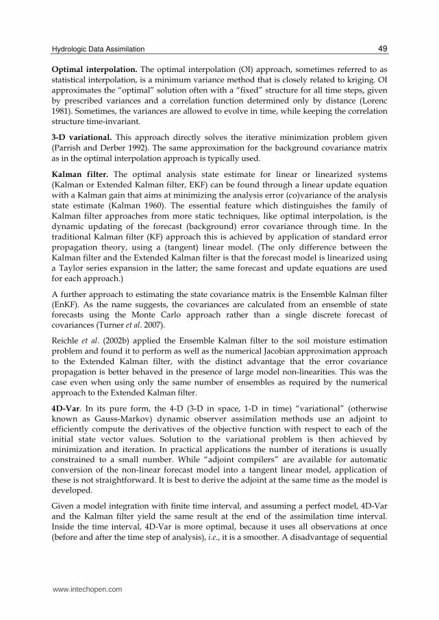
4D-Var. In its pure form, the 4-D (3-D in space, 1-D in time) “variational” (otherwise known as Gauss-Markov) dynamic observer assimilation methods use an adjoint to efficiently compute the derivatives of the objective function with respect to each of the initial state vector values. Solution to the variational problem is then achieved by minimization and iteration. In practical applications the number of iterations is usually constrained to a small number. While “adjoint compilers” are available for automatic conversion of the non-linear forecast model into a tangent linear model, application of these is not straightforward. It is best to derive the adjoint at the same time as the model is developed.

Given a model integration with finite time interval, and assuming a perfect model, 4D-Var

and the Kalman filter yield the same result at the end of the assimilation time interval.

Inside the time interval, 4D-Var is more optimal, because it uses all observations at once

(before and after the time step of analysis), i.e., it is a smoother. A disadvantage of sequential

www.intechopen.com


50

methods is the discontinuity in the corrections, which causes model shocks. Through

variational methods, there is a larger potential for dynamically based balanced analyses,

which will always be situated within the model climatology. Operational 4D-Var assumes a

perfect model: no model error can be included. With the inclusion of model error, coupled

equations are to be solved for minimization. Through Kalman filtering it is in general

simpler to account for model error.

Both the Kalman filter and 3D/4D-Var rely on the validity of the linearity assumption.

Adjoints depend on this assumption and incremental 4D-Var is even more sensitive to

linearity. Uncertainty estimates via the Hessian are critically dependent on a valid

linearization. Furthermore, with variational assimilation it is more difficult to obtain an

estimate of the quality of the analysis or of the state’s uncertainty after updating.

6. Assimilation of hydrologic observations

Estimation of the hydrologic state has mainly been focused on soil moisture, snow water

content, and temperature. The observations used to infer state information range from direct

field measurements of these quantities to more indirectly related measurements like

radiances or backscatter values in remote sensing products. A few studies have also tried to

assimilate state-dependent diagnostic fluxes, like discharge or remotely sensed heat fluxes.

The success of assimilation of observations which are indirectly related to the state is largely

dependent on a good characterization of the observation operator. This section presents

examples of research in hydrologic data assimilation, but is not intended to be a

comprehensive review.

Truly optimal data assimilation techniques require flawless model and observation error

characterization. Therefore, recent studies have focused on the first and second order error

characterization in hydrologic modelling. Typically, either model predictions or

observations are biased. Studies by Reichle and Koster (2004), Bosilovich et al. (2007) and De

Lannoy et al. (2007a, b) scratch the surface of how to deal with these hydrologic modelling

biases. The second order error characterization is of major importance to optimize the

analysis result and for the propagation of information through the system. Tuning of the

error covariance matrices has, therefore, gained attention with the exploration of adaptive

filters in hydrologic modelling (Reichle et al. 2008; De Lannoy et al. 2009).

Furthermore, it is important to understand that hydrologic data assimilation applications

are dealing with non-closure or imbalance problems, caused by external data assimilation

for state estimation. In a first attempt to attack this problem, Pan and Wood (2006)

developed a constrained Ensemble Kalman filter which optimally redistributes any

imbalance after conventional filtering. They applied this technique over a 75,000 km2

domain in the US, using the terrestrial water balance as constraint.

7. Case studies

Significant advances in hydrological data assimilation have been made over the past decade

from which we have selected a few case studies to demonstrate the utility of hydrological

data assimilation in hazard prediction and mitigation.

www.intechopen.com


51

7.1 Case study 1: Assimilation of water level observations

By providing predictions of flood hazard and risk over increasing lead-times, flood

inundation models play a central role in advanced hydro-meteorological forecasting

systems. As the cost of damage caused by flooding is highly dependent on the warning time

given before a storm event, the reduction of its predictive uncertainties has received a great

deal of attention by researchers in recent years (e.g., Montanari et al., 2009, Biancamaria et

al., 2010). The predictive uncertainty originates from several causes interacting between each

other, namely input uncertainty (i.e. inflows), model structure and parameter uncertainty.

The predictive uncertainty can be reduced through a periodical updating of computed water

surface lines by taking advantage of water level measurements. However, ground based

data are spatially rather limited, numbers of hydrometric stations are in decline at a global

scale and major parts of the world still remain largely ungauged to this date. Recent

developments in remotely sensing-based measurement techniques potentially help

overcoming data scarcity. For instance, the technique of water stage retrievals from satellite

measurements with centimeter-scale accuracy (e.g. Alsdorf et al., 2007) can be seen as a

promising alternative to hydrometric station data.

Matgen et al. (2010) demonstrated that the real-time assimilation of remote sensing-

derived water elevation into 1D hydraulic models via a Particle Filter enables the

correction of water depth from a corrupted hydraulic model. In their synthetic

experiments they found that significant model improvements could be achieved with

observation error standard deviations up to 5 m. Another interesting result from their

synthetic experiments is the realization that it is crucial to adjust the fluxes at the

upstream boundaries of the model in order to significantly and persistently improve the

hydraulic model. In river hydraulics, the process time scale is relatively short, so that

stock updates have a limited lifetime. As in Andreadis et al. (2007), the research of Matgen

et al. (2010) has clearly demonstrated that because of the dominating effect of the

upstream boundary condition merely updating the state variable of the model (water

level and hence water storage), only improves the model forecast over a very short time

horizon. Model predictions rapidly degrade after updating if the forcing data are not

consistent with observed water levels. Updating the uncertain upstream boundary

condition leads to more persistent model improvement.

Giustarini et al. (2011) recently tested the methodology with real event data using water

level data obtained from ERS-2 SAR and ENVISAT ASAR during the January 2003 flood of

the Alzette River (Grand-Duchy of Luxembourg). The retrieval of water elevation data from

SAR is based on three steps (see Hostache et al., 2009 for a detailed description of the

method). First, the flood extension limits with their respective geolocation uncertainty are

derived from a SAR image using a radiometric thresholding-based procedure. Next, the

resulting uncertain flood extent limits are superimposed on a digital elevation model (DEM)

in order to estimate local water levels. The method takes into account the uncertainty

stemming from the underlying DEM. The water level information is obtained as model

cross-section specific intervals of the possible local water level. In the last step, the intervals

of water levels are hydraulically constrained in order to reduce the estimation uncertainty

(see Figure 4). The Particle Filter-based assimilation scheme consists in having a single

particle with water levels at all cross sections as state vector. Hence, the likelihood that is

www.intechopen.com


52

computed for each particle is derived from its ability to correctly predict water levels along

the entire river reach. In order to overcome the problem of non-persistent model

improvements, the forcing of the hydraulic model is updated as well, using information on

model error that is obtained during the analysis cycle. The approach works well if inflows

are the main source of error in hydraulic modelling. However, when model behavior is non-

uniform across the model domain, it is preferred to have the Particle Filter assign a separate

particle set to each cross-section. Giustarini et al. (2011) further conclude that the analysis

step is of major importance for carrying out an efficient inflow correction over many time

steps as errors in the analysis will propagate through the inflow correction model, thereby

potentially degrading the skill of the forecasts. The data assimilation experiments show the

potential of remote sensing-derived water level data for persistently improving model

predictions over many time steps (see Figure 5).

Fig. 4. Diagram showing an example of: (a) flood extent derived from a satellite image superimposed on the DEM and the river cross-section location, (b) illustration of water level values extracted for a given cross-section and c) the remote sensing-derived water elevation along a portion of stream (c) before and (d) after applying the hydraulic coherence constrain.

www.intechopen.com


53

Fig. 5. Stage hydrographs at one river cross-section before and after assimilating remote

sensing-derived water level intervals from two SAR images into the 1D hydraulic model

(bottom panel). The forecasting performance is evaluated with the RMSE evolution in time

(top panel). The cyan line represents the RMSE before assimilation and the black line

displays the RMSE after assimilation.

7.2 Case study 2: Assimilation of snow water equivalent and snow cover fraction

Snowmelt runoff is of major importance to summer water supplies, and plays a considerable

role in mid-latitude flood events. Snow alters the interface between the atmosphere and the

land surface through its higher albedo and lower roughness compared to snow-free

conditions, and by thermally insulating the soil from the atmosphere. Consequently, the

presence of snow strongly affects the land surface water and energy balance, weather and

climate. Moreover, snow has a high spatial and temporal variability which is very sensitive

to global change.

www.intechopen.com


54

Numerical simulation of snow processes is far from perfect (Slater et al., 2001), therefore

snow data assimilation could provide a more accurate estimate of snow conditions. Satellite-

based snow cover fraction (SCF) observations are available using visible and near-infrared

measurements from sensors like the Moderate Resolution Imaging Spectroradiometer

(MODIS, 2000 - present). While accurate, these observations have limitations (Dong and

Peters-Lidard, 2010), such as the inability to see through clouds. Additionally, SCF

observations only provide a partial estimate of the snow state, namely snow cover; in

contrast, hydrologic modeling uses snow water equivalent (SWE, snow mass), so snow

depletion curves are used to imperfectly translate SCF to SWE. These SCF issues can be

overcome using SWE observations derived from passive microwave observations such as

the Scanning Multichannel Microwave Radiometer (SMMR, 1978 − 1987), Special Sensor

Microwave Imager (SSM/I, 1987-present) and Advanced Microwave Scanning Radiometer

for the Earth Observing System (AMSR-E, 2002-present). These sensors do not suffer from

cloud obscuration and allow SWE estimation by relating the microwave brightness

temperature to snow parameters, but typically have a much coarser resolution and low

precision (Dong et al., 2005).

Therefore, an improved snow analyses can be expected by combining the strengths of

different snow observations and models. De Lannoy et al. (2011) examined the possibilities

and limitations of assimilating both fine-scale MODIS SCF and coarse-scale AMSR-E SWE

retrievals into the Noah LSM using an EnKF. Eight years (2002−2010) of remotely sensed

AMSR-E snow water equivalent (SWE) retrievals and MODIS snow cover fraction (SCF)

observations were assimilated into the Noah LSM over a domain in Northern Colorado

using a multi-scale ensemble Kalman filter (EnKF), combined with a rule-based update. De

Lannoy et al., 2011 discuss several experiments: (a) ensemble open loop without assimilation

(EnsOL); (b) assimilation of coarse-scale AMSR-E SWE observations (SWE DA); (c)

assimilation of fine-scale MODIS SCF observations (SCF DA), which involves a mapping

from SCF to SWE; and (d) joint, multi-scale assimilation of AMSR-E SWE and MODIS SCF

observations (SWE & SCF DA).

Figure 6 illustrates the spatial patterns of the satellite observations, the EnsOL estimates,

and the assimilation estimates (without scaling) for a few representative days during the

winter of 2009-2010. For this winter, the model and satellite observations have a similar SWE

magnitude and no explicit bias-correction is needed to interpret the spatial patterns. The 3D

filter performs a downscaling of the coarse AMSR-E SWE observations and shows a realistic

fine-scale variability driven by the land surface model integration (De Lannoy et al., 2010).

For example, high elevations maintain SWE values well above the observed AMSR-E SWE,

which would not be the case if the AMSR-E pixels were a priori partitioned and assimilated

with a 1D filter. Furthermore, areas without observations (swath effects) are updated

through spatial correlations in the forecast errors. The 1D SCF filter imposes the fine-scale

MODIS-observed variability, and locations without fine-scale observations (due to clouds)

are not updated. The combined SWE and SCF assimilation shows features of both the SWE

and SCF assimilation integrations. Assimilation and downscaling of coarse-scale AMSR-E

SWE as well as MODIS SCF assimilation maintain realistic spatial patterns in the SWE

analyses.

www.intechopen.com


55

Fig. 6. SWE (at 8:00 UTC) and SCF (at 17:00 UTC) fields at 5 days in the winter of 2009-2010. The top 2 series show the assimilated observations, the other plots show SWE and SCF for the EnsOL forecast and 3 different data assimilation (DA) analyses. AMSR-E data are missing due to the swath effect and MODIS data are missing because of cloud contamination.

www.intechopen.com


56

7.3 Case study 3: Assimilation of soil moisture observations

Soil moisture is an important initialization variable for large-scale weather forecasts and

climate predictions. Smaller-scale soil moisture conditions have a great impact on

agriculture, ecology and hydrology. The occurrence of droughts and flooding has a major

impact on human lives and monitoring the soil moisture helps to prevent or mitigate

disasters. Regional to global soil moisture data rely mostly on land surface model

simulations forced by meteorological data or on satellite-based microwave observations.

However, these satellite observations have coarse spatial resolution, only sense the top few

centimetres of the soil and are only available for a specific area when the satellite happens to

pass over. Through assimilation of these intermittent surface observations into a model,

continuous and consistent soil moisture profile estimates could be obtained.

Liu et al. (2011) illustrated how land surface simulations can be improved by either

improving the precipitation, or by assimilating surface soil moisture retrievals from the

Advanced Microwave Scanning Radiometer (AMSR-E) with a 1-D ensemble Kalman filter

into the NASA Catchment land surface model. The assimilated soil moisture products were

either the operational NASA Level-2B AMSR-E “AE-Land” product (archived by NSIDC), or

the Land Parameter Retrieval Model C-band LPRM-C product. The forcings were based on

the atmospheric forcing fields from Modern Era Retrospective-analysis for Research and

Applications (MERRA), but the precipitation is corrected with large-scale, gauge- and

satellite-based precipitation observations from different datasets (CMAP, GPCP, and CPC).

The soil moisture skill was defined as the anomaly time series correlation coefficient R of the

model or assimilation results against in situ observations in the continental United States at

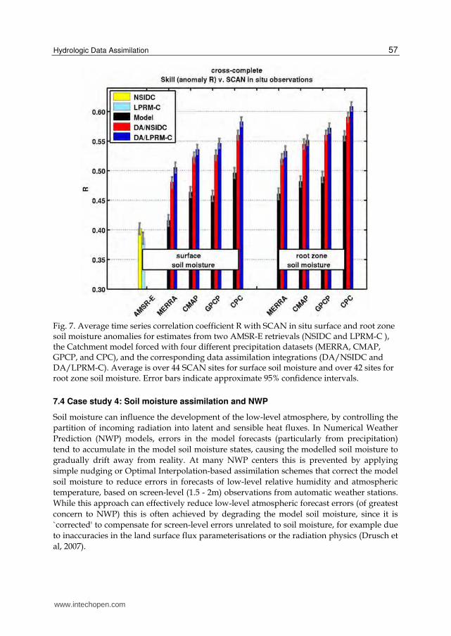
44 single-profile sites within the Soil Climate Analysis Network (SCAN). Figure 7 shows

that the precipitation corrections and assimilation of satellite soil moisture retrievals

contribute comparable and largely independent amounts of information to the assimilation

results. Furthermore, it should be stressed that the satellite observations are only available

for the surface soil layer and assimilation of these surface data clearly helps to improve the

soil moisture estimates in the root zone.

The above example assimilated the coarse-scale AMSR-E data with a 1-D filter and focused

on improving the temporal characteristics of the assimilation results for large scale

applications. In another study by Sahoo et al. (2011), coarse-scale AMSR-E observations

were assimilated with more focus on the fine-scale spatial variability by applying a 3-D

spatial filter (Reichle and Koster, 2003, De Lannoy et al., 2010) to downscale the observations

to the fine-scale model resolution over the Little River Experimental Watershed in Georgia.

A correct assessment of the soil moisture pattern could largely impact flood predictions and

may be crucial in the effective mitigation of droughts. Furthermore, as numerous previous

studies (e.g., Walker et al. (2001b), De Lannoy et al. (2006), Liu et al. (2011)), it was

reconfirmed that the assimilation of surface observations impact the deeper layer soil

moisture and other water balance variables, but Sahoo et al. (2011) also illustrated that

assimilation of surface observations helps the model to spin up faster to its balanced state,

both in the surface and deeper layers. This is shown by the gray arrow in Figure 8, which

indicates the time difference in model spin up without and with data assimilation. Data

assimilation thus better prepares and balances the land surface models to provide improved

short-term soil moisture forecasts.

www.intechopen.com


57

Fig. 7. Average time series correlation coefficient R with SCAN in situ surface and root zone soil moisture anomalies for estimates from two AMSR-E retrievals (NSIDC and LPRM-C ), the Catchment model forced with four different precipitation datasets (MERRA, CMAP, GPCP, and CPC), and the corresponding data assimilation integrations (DA/NSIDC and DA/LPRM-C). Average is over 44 SCAN sites for surface soil moisture and over 42 sites for root zone soil moisture. Error bars indicate approximate 95% confidence intervals.

7.4 Case study 4: Soil moisture assimilation and NWP

Soil moisture can influence the development of the low-level atmosphere, by controlling the

partition of incoming radiation into latent and sensible heat fluxes. In Numerical Weather

Prediction (NWP) models, errors in the model forecasts (particularly from precipitation)

tend to accumulate in the model soil moisture states, causing the modelled soil moisture to

gradually drift away from reality. At many NWP centers this is prevented by applying

simple nudging or Optimal Interpolation-based assimilation schemes that correct the model

soil moisture to reduce errors in forecasts of low-level relative humidity and atmospheric

temperature, based on screen-level (1.5 - 2m) observations from automatic weather stations.

While this approach can effectively reduce low-level atmospheric forecast errors (of greatest

concern to NWP) this is often achieved by degrading the model soil moisture, since it is

`corrected' to compensate for screen-level errors unrelated to soil moisture, for example due

to inaccuracies in the land surface flux parameterisations or the radiation physics (Drusch et

al, 2007).

www.intechopen.com


58

Fig. 8. Sensitivity results of the EnKF 3-D algorithm to the model initialization conditions and model spin-up for the Soil Moisture (a) Layer 1, (b) Layer 2, (c) Layer 3 and (d) Layer 4. The results are spatially averaged over 16 in-situ locations. OL (dashed) stands for the Open Loop model simulation without assimilation, started from different initial soil moisture wetness values. 3D (solid line) refers to assimilation results with L (low), M (moderate) and H (high) initial soil moisture. The simulations start in the summer (July 1, 2002 = S).

Ultimately, inaccurate soil moisture in an NWP model will lead to inaccurate atmospheric forecasts. Additionally, if accurate soil moisture states could be obtained from NWP models, these would be valuable for other operational applications, such as hydrological modelling, flood forecasting, and drought monitoring. A promising solution to improving the accuracy of the soil moisture in NWP models is to make use of novel remotely sensed observations of near-surface soil moisture, such as those available from AMSR-E. Within this context, a study by Draper et al. (2011) presents an Extended Kalman Filter (EKF) capable of assimilating both screen-level observations and remotely sensed near-surface soil moisture

www.intechopen.com


59

observations into an NWP model. This EKF, based on the Simplified EKF of Mahfouf et al (2009), was specifically designed to be computationally affordable within an operational NWP model, however the experiments presented here were conducted using an offline land surface model (with no feedback to the atmospheric model).

A series of assimilation experiments was conducted to compare the EKF assimilation of AMSR-E derived near-surface soil moisture and screen-level observations into Météo-France's NWP model over Europe. Figure 9 demonstrates how assimilating each data set influenced the fit between the subsequent model forecasts and each of the assimilated data sets. When the AMSR-E soil moisture and screen-level observations were assimilated separately, there was no clear consistency between the resulting root-zone soil moisture analyses, and so Figure 9 shows that assimilating one data set did not improve the model fit to the other data set. Hence, for these experiments the screen-level observations could not have been substituted with the AMSR-E data to achieve similar corrections to the low-level atmospheric forecasts, implying that the remotely sensed soil moisture may not be immediately useful for Météo-France's NWP model. However, for the experiments assimilating the screen-level observations the soil moisture innovations were dominated by a diurnal cycle that was not related to the model soil moisture, reinforcing the need to develop the assimilation of alternative data sets.

Fig. 9. Mean daily observation minus model forecast, averaged over Europe, for each day in July 2006, for a) temperature at 2m above the surface, T_2m (K), b) relative humidity at 2m above the surface, RH_2m (%), and c) surface soil moisture, w_1 (m3m-3), for an open-loop (no assimilation; black, solid), assimilation of screen-level variables (black, dashed), assimilation of AMSR-E soil moisture (grey, solid), and assimilation of both data sets (grey, dashed) experiments.

www.intechopen.com


60

When the AMSR-E and screen-level observations were assimilated together, the EKF slightly improved the fit between the model forecasts and both observed data sets, although these improvements were very modest, and the root mean square difference over the one month experiment over all of Europe between the model forecasts and the assimilated observations was reduced by less than 5% of the open-loop values, for all assimilated variables. If this result can be substantiated with larger improvements by performing the assimilation in a fully coupled NWP model, this would confirm that assimilating remotely sensed near-surface soil moisture together with screen-level observations has the potential to improve the realism of the NWP land surface without degrading the low-level atmospheric forecasts.

8. Summary

Hydrological data assimilation is an objective method to estimate the hydrological system states from irregularly distributed observations. These methods integrate observations into numerical prediction models to develop physically consistent estimates that better describe the hydrological system state than the raw observations alone. This process is extremely valuable for providing initial conditions for hydrological system prediction and/or correcting hydrological system prediction, and for increasing our understanding and improving parametrization of hydrological system behaviour through various diagnostic research studies.

Hydrological data assimilation has still many open areas of research. Development of hydrological data assimilation theory and methods is needed to: (i) better quantify and use model and observational errors; (ii) create model-independent data assimilation algorithms that can account for the typical non-linear nature of hydrological models; (iii) optimize data assimilation computational efficiency for use in large operational hydrological applications; (iv) use forward models to enable the assimilation of remote sensing radiances directly; (v) link model calibration and data assimilation to optimally use available observational information; (vi) create multivariate hydrological assimilation methods to use multiple observations with complementary information; (vii) quantify the potential of data assimilation downscaling; and (viii) create methods to extract the primary information content from observations with redundant or overlaying information. Further, the regular provision of snow, soil moisture, and surface temperature observations with improved knowledge of observational errors in time and space are essential to advance hydrological data assimilation. Hydrological models must also be improved to: (i) provide more “observable” land model states, parameters, and fluxes; (ii) include advanced processes such as river runoff and routing, vegetation and carbon dynamics, and groundwater interaction to enable the assimilation of emerging remote sensing products; (iii) have valid and easily updated adjoints; and (iv) have knowledge of their prediction errors in time and space. The assimilation of additional types of hydrological observations, such as streamflow, vegetation dynamics, evapotranspiration, and groundwater or total water storage must be developed.

As with most current data assimilation efforts, we describe data assimilation procedures that are implemented in uncoupled models. However, it is well known that the high-resolution time and space complexity of hydrological phenomena have significant interaction with atmospheric, biogeochemical, and oceanic processes. Scale truncation errors, unrealistic physics formulations, and inadequate coupling between hydrology and

www.intechopen.com


61

the overlying atmosphere can produce feedbacks that can cause serious systematic hydrological errors. Hydrological balances cannot be adequately described by current uncoupled hydrological data systems, because large analysis increments that compensate for errors in coupling processes (e.g. precipitation) result in important non-physical contributions to the energy and water budgets. Improved coupled process models with improved feedback processes, better observations, and comprehensive methods for coupled assimilation are needed to achieve the goal of fully coupled data assimilation systems that should produce the best and most physically consistent estimates of the Earth system.

9. References

Alsdorf, D. E., Rodriguez, E., & Lettenmaier, D. P. (2007). Measuring surface water from space, Reviews of Geophysics, 45, doi:10.1029/2006RG000197.

Andreadis, K. M., Clark, E. A., Lettenmaier, D. P., & Alsdorf, D. E. (2007). Prospects for river discharge and depth estimation through assimilation of swath-altimetry into a raster-based hydrodynamics model, Geophys. Res. Lett., 34, L10403, doi:10.1029/2007GL029721.

Andreadis, K.M. and D.P. Lettenmaier, 2006. Assimilating remotely sensed snow observation into a macroscale hydrology model. Adv. Water Resour., 29, 872–886.

Bennett, A.F., 1992. Inverse methods in physical oceanography. Cambridge University Press, 346 pp. Bergthorsson, P. and B. Döös, 1955. Numerical weather map analysis. Tellus, 7, 329–340. Biancamaria, S., Durand, M., Andreadis, K. M., Bates, P. D., Booneg, A., Mognard, N. M.,

Rodríguez, E., Alsdorf, D. E., Lettenmaier, D. P., & Clark, E. A. (2010). Assimilation of virtual wide swath altimetry to improve Arctic river modelling, Remote Sensing of Environment, doi:10.1016/j.rse.2010.09.008.

Bosilovich, M.G., J.D. Radakovich, A.D. Silva, R. Todling and F. Verter, 2007. Skin temperature analysis and bias correction in a coupled land-atmosphere data assimilation system. J. Meteorol. Soc. Jpn., 85A, 205-228.

Bratseth, A.M., 1986. Statistical interpolation by means of successive corrections. Tellus, 38A, 439-447.

Charney, J.G., M. Halem and R. Jastrow, 1969. Use of incomplete historical data to infer the present state of the atmosphere. J. Atmos. Sci., 26, 1160-1163.

Cressman, G.P., 1959. An operational objective analysis system. Mon. Weather Rev., 87, 367–374. Daley, R., 1991. Atmospheric data analysis. Cambridge University Press, 460 pp. De Lannoy, G.J.M., P.R. Houser, N.E.C. Verhoest and V.R.N. Pauwels, 2009. Adaptive soil

moisture profile filtering for horizontal information propagation in the independent column-based CLM2.0, J. Hydrometeorol., 10(3), 766-779.

De Lannoy, G.J.M., P.R. Houser, V.R.N. Pauwels and N.E.C. Verhoest, 2006. Assessment of model uncertainty for soil moisture through ensemble verification. J. Geophys. Res., 111, D10101.1-18.

De Lannoy, G.J.M., P.R. Houser, V.R.N. Pauwels and N.E.C. Verhoest, 2007b. State and bias estimation for soil moisture profiles by an ensemble Kalman filter: effect of assimilation depth and frequency. Water Resour. Res., 43, W06401, doi:10.1029/2006WR005100.

De Lannoy, G.J.M., R. H. Reichle, K. R. Arsenault, P. R. Houser, S. Kumar, N. E. C. Verhoest, V.R.N. Pauwels, 2011. Multi-Scale Assimilation of AMSR-E Snow Water Equivalent and MODIS Snow Cover Fraction in Northern Colorado, Water Resour. Res., in review.

www.intechopen.com


62

De Lannoy, G.J.M., R.H. Reichle, P.R. Houser, K. R. Arsenault, V.R.N. Pauwels and N.E.C. Verhoest, 2009. Satellite-scale snow water equivalent assimilation into a high-resolution land surface model, J. Hydrometeorol., in press.

De Lannoy, G.J.M., R.H. Reichle, P.R. Houser, V.R.N. Pauwels and N.E.C. Verhoest, 2007a. Correcting for forecast bias in soil moisture assimilation with the ensemble Kalman filter. Water Resour. Res., 43, W09410, doi:10.1029/2006WR00544.

De Lannoy, G.J.M., Reichle, R.H., Houser, P.R., Arsenault, K., Verhoest, N.E.C., Pauwels, V.R.N. (2011). Multi-Scale Assimilation of AMSR-E Snow Water Equivalent and MODIS Snow Cover Fraction in Northern Colorado, Water Resources Research, conditionally accepted.

Déry, S.J., V.V. Salomonson, M. Stieglitz, D.K. Hall and I. Appel, 2005. An approach to using snow areal depletion curves inferred from MODIS and its application to land surface modelling in Alaska. Hydrol. Processes, 19, 2755–2774.

Dirmeyer, P., 2000. Using a global soil wetness dataset to improve seasonal climate simulation. J. Climate, 13, 2900–2921.

Dong, J., and C. Peters-Lidard (2010). On the Relationship Between Temperature and MODIS Snow Cover Retrieval Errors in the Western U.S. IEEE Trans. Geosci. Remote Sens., 3(1), 132-140.

Dong, J., J.P. Walker and P.R. Houser, 2005. Factors Affecting Remotely Sensed Snow Water Equivalent Uncertainty. Remote Sensing of Environment, 97, 68-82, doi:10.1016/j.rse.2005.04.010.

Dong, J., J.P. Walker, P.R. Houser and C. Sun, 2007. Scanning multichannel microwave radiometer snow water equivalent assimilation. J. Geophys. Res., 112, D07108, doi:10.1029/2006JD007209.

Draper, C. S., J.-F. Mahfouf, and J. P. Walker (2011), Root zone soil moisture from the assimilation of screen-level variables and remotely sensed soil moisture, J. Geophys. Res., 116, D02127, doi:10.1029/2010JD013829.

Drusch, M. and Viterbo, P. (2007). Assimilation of screen-level variables in ECMWF’s Integrated Forecast System: A study on the impact on the forecast quality and analyzed soil moisture, Monthly Weather Review, 135, 300-314.

Giustarini, L., Matgen, P., Hostache, R., Montanari, M., Plaza, D., Pauwels, V. R. N., De Lannoy, G. J. M., De Keyser, R., Pfister, L., Hoffmann, L, & Savenije, H. H. G. (2011). Assimilatign SAR-derived water level data into a flood models: a case study, Hydrol. Earth Syst. Sci., 15, 2349-2365.

Hostache, R., Matgen, P., Schumann, G., Puech, C., Hoffmann, L., & Pfister, L. (2009). Water level estimation and reduction of hydraulic model calibration uncertainties using satellite SAR images of floods, IEEE Transactions on Geoscience and Remote Sensing, 47, 431-441.

Houser, P., M.F. Hutchinson, P. Viterbo, J. Hervé Douville and S.W. Running, 2004. Terrestrial data assimilation, Chapter C.4 in Vegetation, Water, Humans and the Climate. Global Change - The IGB Series. Kabat, P. et al. (eds). Springer, Berlin, pp 273-287.

Houser, P.R., W.J. Shuttleworth, J.S. Famiglietti, H.V. Gupta, K.H. Syed and D.C. Goodrich, 1998. Integration of soil moisture remote sensing and hydrologic modeling using data assimilation. Water Resour. Res., 34, 3405-3420.

Hu, Y., X. Gao, W. Shuttleworth, H. Gupta and P. Viterbo, 1999. Soil moisture nudging experiments with a single column version of the ECMWF model. Q. J. R. Meteorol. Soc., 125, 1879–1902.

www.intechopen.com


63

Kalman, R.E., 1960. A new approach to linear filtering and prediction problems. Trans. ASME, Ser. D, J. Basic Eng., 82, 35-45.

Koster, R.D., M. Suarez, P. Liu, U. Jambor, A. Berg, M. Kistler, R. Reichle, M. Rodell and J. Famiglietti, 2004. Realistic initialization of land surface states: Impacts on subseasonal forecast skill. J. Hydrometeorol., 5, 1049–1063.

Kostov, K.G. and T.J. Jackson, 1993. Estimating profile soil moisture from surface layer measurements – A review. In: Proc. The International Society for Optical Engineering, Vol. 1941, Orlando, Florida, pp 125-136.

Liu, Q., Reichle, R.H., Bindlish, R., Cosh, M.H., Crow, W. T., de Jeu, R., De Lannoy, G.J.M., Huffman, G.J., Jackson, T.J. (2011). The contribution of precipitation forcing and satellite observations of soil moisture on the skill of soil moisture estimates in a land data assimilation system, Journal of Hydrometeorology, in press.

Lorenc, A., 1981. A global three-dimensional multivariate statistical interpolation scheme. Mon. Weather Rev., 109, 701-721.

Lorenc, A.C., R.S. Bell and B. Macpherson, 1991. The Meteorological Office analysis correction data assimilation scheme. Q. J. R. Meteorol. Soc., 117, 59-89.

Mahfouf, J.-F., Bergaoui, K., Draper, C., Bouyssel, C., Taillefer, F. and Taseva, L. (2009). A comparison of two off-line soil analysis schemes for assimilation of screen-level observations, Journal of Geophysical Research, 114, D08105.

Margulis, S.A., E.F. Wood and P.A. Troch, 2006. A terrestrial water cycle: Modeling and data assimilation across catchment scales. J. Hydrometeorol., 7, 309–311.

Matgen, P., Montanari, M., Hostache, R., Pfister, L., Hoffmann, L., Plaza, D., Pauwels, V. R. N., De Lannoy, G. J. M., De Keyser, R., & Savenije, H. H. G. (2010). Towards the sequential assimilation of SAR-derived water stages into hydraulic models using the Particle Filter: proof of concept, Hydrol. Earth Syst. Sci., 14, 1773-1785.

McLaughlin, D., 1995. Recent developments in hydrologic data assimilation. In U.S. National Report to the IUGG (1991-1994). Rev. Geophys., supplement, 977–984.

McLaughlin, D., 2002. An integrated approach to hydrologic data assimilation: interpolation, smoothing, and filtering. Adv. Water Resour., 25, 1275–1286.

Montanari, M., Hostache, R., Matgen, P., Schumann, G., Pfister, L., & Hoffmann, L. (2009). Calibration and sequential updating of a coupled hydrologic-hydraulic model using remote sensing-derived water stages, Hydrol. Earth Syst. Sci., 13, 367-380.

Nichols, N.K., 2001. State estimation using measured data in dynamic system models, Lecture notes for the Oxford/RAL Spring School in Quantitative Earth Observation.

Pan, M. and E.F. Wood, 2006. Data assimilation for estimating the terrestrial water budget using a constrained ensemble Kalman filter. J. Hydrometeorol., 7, 534–547.

Parrish, D. and J. Derber, 1992. The National Meteorological Center’s spectral statistical interpolation analysis system. Mon. Weather Rev., 120, 1747-1763.

Reichle, R.H. and R. Koster, 2003. Assessing the impact of horizontal error correlations in background fields on soil moisture estimation. J. Hydrometeorol., 4, 1229–1242.

Reichle, R.H. and R. Koster, 2004. Bias reduction in short records of satellite soil moisture. Geophys. Res. Lett., 31, L19501.1–L19501.4.

Reichle, R.H., D.B. McLaughlin and D. Entekhabi, 2002a. Hydrologic data assimilation with the ensemble Kalman filter. Mon. Weather Rev., 120, 103–114.

Reichle, R.H., J.P. Walker, P.R. Houser and R.D. Koster, 2002b. Extended versus ensemble Kalman filtering for land data assimilation. J. Hydrometeorol., 3, 728–740.

www.intechopen.com


64

Reichle, R.H., W.T. Crow and C.L. Keppenne, 2008. An adaptive ensemble Kalman filter for soil moisture data assimilation, Water Resour. Res., 44, W03423, doi:10.1029/2007WR006357.

Rood, R.B., S.E. Cohn and L. Coy, 1994. Data assimilation for EOS: The value of assimilated data, Part 1. The Earth Observer, 6, 23-25.

Sahoo, A.K., De Lannoy, G.J.M., Reichle, R.H. (2011). Downscaling of AMSR-E soil moisture in the Little River Watershed, Georgia, USA. Advances in Water Resources, in review.

Sellers, P. J., Y. Mintz, and A. Dalcher, 1986: A simple biosphere model (SiB) for use within general circulation models. J. Atmos. Sci., 43: 505-531.

Slater, A.G. and M. Clark, 2006. Snow data assimilation via an ensemble Kalman filter. J. Hydrometeorol., 7, 478–493.

Stauffer, D.R. and N.L. Seaman, 1990. Use of four-dimensional data assimilation in a limited-area mesoscale model. Part I: Experiments with synoptic-scale data. Mon. Weather Rev., 118, 1250-1277.

Stieglitz, M., D. Rind, J. Famiglietti and C. Rosenzweig, 1997. An efficient approach to modeling the topographic control of surface hydrology for regional and global climate modeling. J. Climate, 10, 118–137.

Turner, M.R.J., J.P. Walker and P.R. Oke, 2007. Ensemble Member Generation for Sequential Data Assimilation. Remote Sensing of Environment, 112, doi:10.1016/j.rse.2007.02.042.

van Loon, E.E. and P.A. Troch, 2001. Directives for 4-D soil moisture data assimilation in hydrological modelling. IAHS, 270, 257-267.

Walker J.P. and P.R. Houser, 2001. A methodology for initialising soil moisture in a global climate model: assimilation of near-surface soil moisture observations, J. Geophys. Res., 106, 11,761-11,774.

Walker, J.P. and P.R. Houser, 2004. Requirements of a global near-surface soil moisture satellite mission: Accuracy, repeat time, and spatial resolution. Adv. Water Resour., 27, 785-801.

Walker, J.P. and P.R. Houser, 2005. Hydrologic data assimilation. In A. Aswathanarayana (Ed.), Advances in water science methodologies (230 pp). The Netherlands, A.A. Balkema.

Walker, J.P., G.R. Willgoose and J.D. Kalma, 2001a. One-dimensional soil moisture profile retrieval by assimilation of near-surface observations: A comparison of retrieval algorithms. Adv. Water Resour., 24, 631-650.

Walker, J.P., G.R. Willgoose and J.D. Kalma, 2001b. One-dimensional soil moisture profile retrieval by assimilation of near-surface measurements: A simplified soil moisture model and field application. J. Hydrometeorol., 2, 356-373.

Walker, J.P., G.R. Willgoose and J.D. Kalma, 2002. Three-dimensional soil moisture profile retrieval by assimilation of near-surface measurements: Simplified Kalman filter covariance forecasting and field application. Water Resour. Res., 38, 1301, doi:10.1029/2002WR001545.

Walker, J.P., P.R. Houser and R. Reichle, 2003. New technologies require advances in hydrologic data assimilation. EOS, 84, 545–551.

WMO, 1992. Simulated real-time intercomparison of hydrological models (Tech. Rep. No. 38). Geneva.

Zhang, H. and C.S. Frederiksen, 2003. Local and nonlocal impacts of soil moisture initialization on AGCM seasonal forecasts: A model sensitivity study. J. Climate, 16, 2117–2137.

www.intechopen.com

Approaches to Managing Disaster - Assessing Hazards,Emergencies and Disaster ImpactsEdited by Prof. John Tiefenbacher

ISBN 978-953-51-0294-6Hard cover, 162 pagesPublisher InTechPublished online 14, March, 2012Published in print edition March, 2012

InTech EuropeUniversity Campus STeP Ri Slavka Krautzeka 83/A 51000 Rijeka, Croatia Phone: +385 (51) 770 447 Fax: +385 (51) 686 166www.intechopen.com

InTech ChinaUnit 405, Office Block, Hotel Equatorial Shanghai No.65, Yan An Road (West), Shanghai, 200040, China

Phone: +86-21-62489820 Fax: +86-21-62489821

Approaches to Managing Disaster - Assessing Hazards, Emergencies and Disaster Impacts demonstrates thearray of information that is critical for improving disaster management. The book reflects major managementcomponents of the disaster continuum (the nature of risk, hazard, vulnerability, planning, response andadaptation) in the context of threats that derive from both nature and technology. The chapters include aselection of original research reports by an array of international scholars focused either on specific locationsor on specific events. The chapters are ordered according to the phases of emergencies and disasters. Thetext reflects the disciplinary diversity found within disaster management and the challenges presented by theco-mingling of science and social science in their collective efforts to promote improvements in the techniques,approaches, and decision-making by emergency-response practitioners and the public. This text demonstratesthe growing complexity of disasters and their management, as well as the tests societies face every day.

How to referenceIn order to correctly reference this scholarly work, feel free to copy and paste the following:

Paul R. Houser, Gabriëlle J.M. De Lannoy and Jeffrey P. Walker (2012). Hydrologic Data Assimilation,Approaches to Managing Disaster - Assessing Hazards, Emergencies and Disaster Impacts, Prof. JohnTiefenbacher (Ed.), ISBN: 978-953-51-0294-6, InTech, Available from:http://www.intechopen.com/books/approaches-to-managing-disaster-assessing-hazards-emergencies-and-disaster-impacts/land-surface-data-assimilation

© 2012 The Author(s). Licensee IntechOpen. This is an open access articledistributed under the terms of the Creative Commons Attribution 3.0License, which permits unrestricted use, distribution, and reproduction inany medium, provided the original work is properly cited.

http://creativecommons.org/licenses/by/3.0

hydrologic data assimilation - intech - open science open

Documents