hydrological snowmelt modelling in snow covered … · 3.2 water balance and snowmelt-runoff...
TRANSCRIPT

Hydrological Snowmelt Modelling in Snow Covered River Basins
By Means of Geographic Information System and Remote Sensing
Case Study -- Latyan Catchment in Iran
Dissertation zur Erlangung des akademischen Grades doctor rerum naturalium
(Dr. rer.nat.)
vorgelegt dem Rat der Chemisch-Geowissenschaftlichen Fakultät der
Friedrich-Schiller-Universität Jena von Master-Geographer Houshang Behrawan
geboren am 20. März 1972 in Mahabad, Iran

1. Gutachter: Prof. Dr. rer. nat. Wolfgang-Albert Flügel, Jena
2. Gutachter: Univ. Prof. Dr. rer. nat. Volker Hochschild, Tübingen
Tag der öffentlichen Verteidigung: 08.07.2010

To my dears, Snoor and Chawan and to those who are always in my mind.

I
Contents
LISTS OF FIGURES ................................................................................................................ V LISTS OF TABLES ................................................................................................................VII ABBREVIATIONS............................................................................................................... VIII Abstract ....................................................................................................................................XI 1. Introduction ........................................................................................................................ 1
1.1 OBJECTIVE............................................................................................................... 3 2. Research Review ................................................................................................................ 5
2.1 Snow in the hydrological cycle .................................................................................. 6 2.1.1 Defintion of Snow .............................................................................................. 8 2.1.2 Snow density ...................................................................................................... 8 2.1.3 Snow depth....................................................................................................... 10
2.2 Snow water equivalent (SWE) ................................................................................. 10 2.3 Snowmelt.................................................................................................................. 12
2.3.1 Effect of rainfall, topography and landcover on snowmelt .............................. 14 2.4 Implications of snow-hydrological process dynamics ............................................. 15 2.5 Snow modelling........................................................................................................ 17
2.5.1 Snow-hydrological modelling approaches ....................................................... 20 2.5.1.1 Conceptual outlines of snow-hydrologic modelling approaches ..................... 21 2.5.1.2 Spatial differentiation in the snow- hydrological modelling............................ 23 2.5.1.3 Model-technical coverage of the snow accumulation ...................................... 24
2.6 Snow modelling and water resources....................................................................... 25 2.7 Previous Researches in the Latyan catchment ......................................................... 27
3. METHODICAL APPROACH ......................................................................................... 30 3.1 Hydrological System Analysis and Delineation of Hydrological Response Units .. 31
3.1.1 Hydrological System Analysis ......................................................................... 31 3.1.1.1 Data Analysis of Hydro-Climatological Time Series ...................................... 31 3.1.1.2 Spatial Data Modelling..................................................................................... 32 3.1.2 Delineation of Hydrological Response Units................................................... 33 3.1.2.1 Concept Approach of Hydrological Response Units ....................................... 34
3.2 Water Balance and snowmelt-Runoff Modelling with J2000g Model .................... 35 3.2.1 The Structure of Modelling System of the J2000G Model .............................. 35 3.2.1.1 The Snow Module of the J2000g ..................................................................... 38 3.2.2 Preparation of Input Data ................................................................................. 39 3.2.3 Parameterization and Calibration ..................................................................... 41 3.2.3.1 Automatic Parameter Estimation using Sensitivity Analysis........................... 42
4. STUDY AREA AND DATA BASE................................................................................ 46 4.1 Study Area................................................................................................................ 49
4.1.1 Climatic Condition ........................................................................................... 49 4.1.2 Geomorphology................................................................................................ 52 4.1.2.1 Slope................................................................................................................. 52 4.1.2.2 Aspect............................................................................................................... 53 4.1.3 Landcover/Landuse .......................................................................................... 54 4.1.4 Geology ............................................................................................................ 55 4.1.5 Soil ................................................................................................................... 56
4.2 Data Base.................................................................................................................. 58 4.2.1 Hydro-meteorological datasets......................................................................... 58 4.2.1.1 Precipitation Data ............................................................................................. 58

II
4.2.1.2 Temperature Data ............................................................................................. 59 4.2.1.3 Additional Climatic Parameters ....................................................................... 60 4.2.1.4 Runoff Data ...................................................................................................... 62 4.2.2 Spatial Datasets (GIS-Data) ............................................................................. 62
5. RESULTS AND DISCUSSION ...................................................................................... 64 5.1 System Analysis and Delineation of Hydrological Response Units ........................ 65
5.1.1 Data Analysis and System Analysis................................................................. 65 5.1.1.1 Precipitation Data Analysis .............................................................................. 65 5.1.1.2 Discharge Data Analysis .................................................................................. 66 5.1.1.3 Temporal Relationship between Precipitation and Discharge in the Latyan Catchment......................................................................................................................... 67 5.1.2 Spatial Dataset.................................................................................................. 69 5.1.3 Delineation of Hydrological Response Units................................................... 70 5.1.3.1 Data Preparation and Reclassification.............................................................. 70 5.1.3.2 Overlay Analysis and Reclassification ................................................... 74 5.1.3.3 Generalization and Delineation ........................................................................ 74
5.2 Snowmelt–Runoff Modelling using J2000g model ................................................. 74 5.2.1 Model Parameterization ................................................................................... 74 5.2.1.1 Landuse-Land Cover Information.................................................................... 75 5.2.1.2 Information on Soil Data.................................................................................. 75 5.2.1.3 Information on Geology Data .......................................................................... 76 5.2.2 Model application, calibration and evaluation ................................................. 77 5.2.2.1 Model application............................................................................................. 77 5.2.2.2 Validation ......................................................................................................... 78 5.2.2.3 Verification of the Modeling Results ............................................................... 83
6. CONCLUSIONS AND FUTURE RESEARCH.............................................................. 90 6.1 Conclusions and Future Research ............................................................................ 91
REFERENCES......................................................................................................................... 94 APPENDIX ............................................................................................................................ 110

III
Acknowledgment
At this point, I want to take the chance to thank all those people who have directly or
indirectly contributed to the successful fulfilment of this work. Without the support, guidance
and patience of the following people this work would not have been possible.
First of all, I would like to express my deepest gratefulness to my supervisor and doctor father
Prof. Dr. Wolfgang-Albert Flügel who gave me the opportunity to write this dissertation in
Jena and for his guidance, support and advice over the last years. Again thank you so much in
advance for all. I am also grateful to Prof. Dr. Volker Hochschild who supported this work.
The discussions with him lead to the ideas that are presented in this work.
My cordial thanks go to Dr. Peter Krause, which every time his office was open for my
solving problems and discussions with him helped me a lot to work through the technical as
well as some challenging argumentative problems with my study. His constructive criticism
helped me to focus my ideas and to describe them more clearly. I am also thankful to him for
reading the some part of thesis draft within a short time period.
I appreciate the support of the Ministry of Science, Research and Technology of Iran and
Ministry of Agriculture of Iran, without whose support I could not have done my PhD in
Germany.
I am very grateful to all my colleagues of the Department for Geoinformatics, Hydrology and
Modelling, especially, Dr. Manfred Fink, Dr. Sven Kralisch, Dr. Jörg Helmschrot, Björn
Pfennig, Markus Wolf, Markus Reinhold, Christian Fischer, Franziska Zander, Christian
Schwartze, Marcel Wetzel, Daniel Varga, Frank Bäse, Hannes Müller Schmied who have
given their time to discuss pieces of my work with me and who have also offered valuable
advice. Special thanks also go to Rainer Hoffmann, the system administrator, who helped
with any occurring technical problem.
I am grateful to my friends and colleagues, Markus Reinhold, Dr. Shamsuddin Shahid, Dr.
Timothy Steele and Amanpreet Singh for proofreading and their constructive comments to
improve this dissertation.
Thanks to all agencies and institutes providing data and various support for this study: to the
AREEO staffs, in particular, Prof. Dr. Ali Ahoonmanesh, Dr. Bahram Saghafian, Dr. Kazemi,
Mr. Akbarpour, to the Iran Water Resource Management Company (IWRMCO), in particular
to Mr. Babaee, to the Iranian Revenue Operation of Dams, in particular Mr. Engineer

IV
Shahryari, to the Company of Water and Soil Engineering Service Iran (CWSESI), especially
Dr. Parehkar, Engineer Bazzaz, to the Organization of Forests and Rangelands Iran for
providing the land-cover data, to the Dr. Hossein Zeinivand in the University of Lorestan for
providing of various maps and texts of the Roodak watershed.
I would like to extend my sincere gratitude to Mrs. Dorothee Flügel for infinite supporting me
and my family throughout this whole endeavour. I would not have gone so far without her
unfailing support and encouragement.
Many thank for short but very valuable financial support from the Jenaer Graduate Academy
the University of Friedrich-Schiller Jena.
I want to thank all my friends -- in particular, Dr. Osman Azizi, Ebrahim Amini, Dr. Ebrahim
Fattahi, Engineer David Alamshah, Dr. Mousa Kamanroodi, Dr. Farhad Azizpour, Dr. You
Qinglong, Santosh Nepal and Engineer Taher Pasbani.
My sincere thanks to my father-in-low, that without his continuous and encouraging support I
could not finish my PhD.
Special thanks go to my dear parents and to my sisters and brothers for their endless support
and the trust in me.
The making of the thesis was dominated by a time full of privation, not only for the author,
but especially for my family. The success and continuity of the work originated form the
never ending support of them. Many thanks go especially to my wife, who had to suffer under
the evening and weekends full of work. Through her understanding and loving nature and her
encouragements, she helped to finish this work successfully.

V
LISTS OF FIGURES
Figure 1.1: Increasing pattern of water extraction from various catchments including the
Latyan for water supply to the Tehran 02
Figure2-1: The Global Water Cycle 07
Figure 2-2: The Global freshwater and role of snow 07
Figure 2-3: Schematic representation of typical hydrograph curves of melt runoff in selected
Central European region 16
Figure 2-4:The long term of Snow depth and SWE in Shemshak station, Latyan catchment 25
Figure 2-5: Anomaly of snow cover extent in North Hemisphere 26
Figure 3-1: The Concept of Modelling System of the J2000g Model 36
Figure 4-1: Geographical Location of the Latyan catchment 47
Figure 4-2: Streams and Network and Subcatchments of the Latyan Catchment 49
Figure4-3: Mean Annual (1967-2007) Monthly Precipitation in the Latyan Catchment 51
Figure 4-4: Mean Annual (1967-2007) Monthly Precipitation in the Latyan Catchment 51
Figure 4-5: Slope Classes in the Latyan Catchment 53
Figure 4-6: exposition condition of the Latyan Catchment 54
Figure 4-7: Landcover/Landuse of the Latyan Catchment 55
Figure 4-8: Soil Types Map of the Latyan Catchment 57
Figure4-9:The Location of Meteorological stations inside and around the Latyan catchment59
Figure5-1: Dubble Curve Mass Analysis in the Latyan Catchment 66
Figure 5-2: The 34 years Evaluations of rainfall and Runoff in the Latyan catchment 67
Figure 5-3: The34 years Monthly Average of rainfall and runoff in the Latyan Catchment 68
Figure 5-4: Flow-chart of the Delineation of HRUs for the J2000g model 70
Figure 5-5:Result of the validation of J2000g for Roodak subbasin in the Latyan catchment79
Figure 5-6: Monthly precipitation, mean air temperature, snow water equivalent and
snowmelt, Roodak subbasin, J2000g model simulation, 1992-1993. 82
Figure 5-7: Monthly precipitation, mean air temperature, snow water equivalent and
snowmelt, Roodak subbasin, J2000g model simulation, 2000-2001 82
Figure5-8: Graphical comparison between simulated and observed Runoff at Roodak
subcatchment in the Latyan catchment, from 10.1990 through 09.2001 83
Figure 5-9: Mean Annual Runoff. Modelled using the J2000g Model 84
Figure 5-10: Mean Annual Actual Evapotranspiration. Modelled using the J2000g Model 85

VI
Figure 5-11: Mean Annual (1990-2001) Snow Water Equivalent (SWE) Modelled using the
J2000g Model 87
Figure 5-12: Mean Annual Temperature (1990-2001) modelled using J2000g model in the
Latyan Catchmet 88
Figure 5-13: snowmelt in the high elevation areas of the Alborz Mountains 89

VII
LISTS OF TABLES
Table 3-1:Input Data files of J2000g Model 40
Table 3-2: J2000g parameters and feasible parameter range for monthly 43
Table 4-1: Temperature Measurement Stations 60
Table 4-2: Additional Clamatic Parameters 61
Table 4-3: GIS-dataset for HRU- delineation 63
Table 5-1: Reclassify the aspect 71
Table 5-2 Classification of the Soil Types 71
Table5-3: Classification of the Land Cover Classes 72
Table 5-4: Stage of Geology Classification 72
Table 5-5: Parameters of the Soil Classes for the Soil Water Module 76
Table 5-6: Parameters of the Geology classes for the Ground Water Module 76
Table 5-7: SubCatchment areas, J2000g parameter values from Monte-Carlo-Analysis and
SCE optimisation 80
Table5-8: Water Balance Components for the Entire Modelled Period (1990-2001) 86

VIII
ABBREVIATIONS
ABBREVIATION DESCRIPTION
AC Air Capacity
AET Actual Evapotranspiration
Alb Albedo
ASA Aggregated Simulation Area
AVE Absolute Volume Error
AVG Average
D Depth
DHI Danish Hydraulic Institute
E East
FAO Food and Agriculture Organization of the United Nations
FCA Field Capacity Adaption
GCM General Circulation Model
GIS Geographical Information System
GSI Geological Survey Organization Iran
HRU Hyrological Response Units
HBV Hydrologiska Byråns Vattenbalansavdelning model
HEC-1 Hydrologic Engineering Center
HSPF Hydrological Simulation Program - FORTRAN
ICSI International Commission on Snow and Ice
IDW Inverse Distance Weighting
IPCC Intergovernmental Panel on Climate Change
ISRIC International Soil Reference and Information Centre
IWRMCO Iran Water Resource Management Company
JAMS Jena Adaptable Modeling System
LAI Leaf Area Index
LAT Latitude
Log.NSE Logarithmic Nash-Sutcliffe Efficiency
LON Longitude
LSS Land cover Soil Sets

IX
MAP Mean Annual Precipitation
MAR Mean Annual Runoff
MASL Meter Above See Level
MCM Million Cubic Meter
MMS Modular Modeling System
N North
NCC National Cartographic Center
NSE Nash Sutclif
OBS Observation
P Precipitation
PBIAS relative percentage volume error
PET Potential Evapotranspiration
PRMS Precipitation-Runoff Modeling System
Q Discharge
R² coefficient of determination
Rd Roothing Depth
Rhum Relative Humidity
RS Remote Sensing
RU Response Unit
S South
SC Soil Class
SIM Simulation
SLURP Semi-distributed Land Use-based Runoff Processes
SMHI Swedish Meteorological and Hydrological Institute
SRTM Shuttle Radar Topography Mission
SRM Snow Runoff Model
STDEVP Standard Deviation Population
SUN Sunshine duration
SVAT Soil-Vegetation-Atmosphere-Transfer
SWE Snow Water Equivalent
SWRI Soil Water Research Institute
TIN triangulated irregular network

X
TS Topography Sets
TWRCO Tehran Water Regional Company
USGS US Geological Survey
UTM Universal Transverse Mercator
VSC Vegetation Soil Complex
W West
WASIM Water balance Simulation Model
WEI Water and Energy Institute
WMO World Meteorological Organization
WRB World Reference Base for Soil Resources
WSIMO Weather Service Iran Meteorological Organization
XI
Abstract
In mountainous watersheds snow melt can have a significant impact on the water balance and
at certain times of the year it could be the most important contribution to runoff. In many
parts of the world snow act as natural reservoirs that can play an important role for water
supply. Alas, despite its importance, many of snow driven basins suffer from a lack of
hydrological infrastructure and equipment so they cannot be described adequately in terms of
snow hydrological dynamics. Because of limited accessibility are the few observation stations
in such areas very rarely located in the higher elevations but are concentrated mostly in the
middle and low elevation resulting in an underrepresentation in data availability of the high
altitudes which are important for the process dynamics. Thus the modelling of snow
hydrological dynamics in mountainous regions such as the Latyan catchment is often difficult.
Reasons for this are in addition to the aforementioned data availability, topographic effects
and gradients that can make a spatial interpolation of the input data and the model states a
complicated task.
Especially in semi-arid regions, high-altitude headwater basins with a significant snow
component have a large potential by balancing and distributing scarce water resources.
Particular here, a quantitative assessment of the spatial distribution of snow cover and snow
processes are an important basis for a sound water management and for the hydrological
forecasting and risk prevention. Therefore, the water management in such regions could
benefit from reliable predictions of the hydrological dynamics derived from model based
studies. Suitable models should represent the physical basis and hydrological processes that
simulate the system’s response, fairly well.
In this study the spatially distributed process-oriented hydrological model J2000g was used
for the 700 km² large Latyan catchment in Iran. The target was to derive spatially distributed
estimates of the quantity and timing of hydrological balance terms and state variables like
rainfall, actual evapotranspiration (AET), runoff, snow water equivalent (SWE) and snow
melt. The model uses the distribution concept of Hydrological Response Units (HRU) to take
the spatial variability in the basin into account. The model simulates for each HRU and each
time step snow accumulation and snow melt, soil water content, the actual evapotranspiration,
groundwater recharge and runoff generation distributed into two components – direct runoff
and ground water runoff. The fact that J2000g cannot account for anthropogenetic influences

XII
and natural water losses as they occur in karsts regions made the selection of suitable sub-
basin for model calibration a difficult task. However, three sub-basins Roodak, Najarkola and
Naran could be identified which underground is characterized mainly by impervious bed rock
and which have only minimal anthropogenic influences. The sizes of the three sub-basins are
between 31 to 430 km². For each of these sub-basins, the model parameters were calibrated
automatically by means of Monte-Carlo analysis and the Shuffled Complex Evolution (SCE-
UA) calibration procedure. The calibration was done by the comparison with measured runoff
values for the period from October 1990 to September 2001 in monthly time steps using the
Nash-Sutcliffe efficiency as the objective function. In addition, for each sub-basin the spatial
distribution of rainfall, runoff, actual evapotranspiration, snow melt and snow water
equivalent was analysed and compared with corresponding measurements.
The snow module of the J2000g model was developed and checked against measured values
of nine snow observation stations, which were located within the test basins. For each of the
observation stations the corresponding HRUs were extracted and separate models calibrated
were calibrated using the measured SWE. The model quality was quantified by using the
Nash-Sutcliffe efficiency (NSE) and the coefficient of determination (r²) as objective
functions. The comparison with the calibrated catchment models showed that accumulation
and melting of the snowpack could be simulated reasonably well at all stations but the results
were less good than those of the separately calibrated catchment models.
The comparison of the separate SWE models resulted in values between 0.28 - 0.68 for NSE
and values between 0.53 - 0.83 for r². For the catchment models the comparison of the
simulated runoff with measured data showed NSE values between 0.78 and 0.82. By these
values it can be stated that the hydrological dynamics and the snow processes of the three sub-
basins within the Latyan catchment could be simulated sufficiently well with J2000g. Finally,
a "global" parameter set for whole the Latyan catchment was generated by an area-weighted
mean of the parameters from the calibrated sub-basin models. With this parameter set Nash-
Sutcliffe efficiencies between 0.68 and 0.79 could be obtained for Latyan.
It can be summarized that the single modules and in particular the snow components of
J2000g along with the HRU distribution approach can be considered as suitable for the given
project objectives i.e. the assessment of the hydrological dynamics of the Latyan catchment.

XIII
Hereby, the model can be used to elaborate important hydrological information for a
sustainable management of the water resources.

XIV
Kurzfassung
In gebirgigen Einzugsgebieten kann die Schneeschmelze einen entscheidenden Einfluss auf
die Wasserbilanz haben und zu gewissen Zeiten im Jahr der wichtigste Beitrag zur
Abflussbildung sein. In vielen Teilen der Welt stellen Schneedecken natürliche Speicher dar,
die eine wichtige Rolle für die Wasserversorgung einnehmen können. Trotz ihrer großen
Bedeutung leiden aber viele dieser schneebeeinflussten Einzugsgebiete an einer mangelhaften
hydrologischen Infrastruktur und Ausstattung wodurch sie hinsichtlich der
schneehydrologischen Dynamik nur unzureichend beschrieben werden können. Aus Gründen
der Erreichbarkeit sind die wenigen Beobachtungsstationen in solchen Gebieten nur sehr
selten in den höheren Lagen lokalisiert sondern meist in den mittleren und geriengeren Höhen
konzentriert wodurch die für die Dynamik wichtigen Hochlagen hinsichtlich der
Datenverfügbarkeit unterrepräsentiert sind. Hierdurch ist die Modellierung der
schneehydrologischen Dynamik in gebirgigen Regionen wie dem Latyan Einzugsgebiet oft
schwierig. Gründe hierfür sind neben der bereits angesprochenen Datenverfügbarkeit auch
topographische Effekte und Gradienten, die eine räumliche Interpolation der Eingangsdaten
und der Modellzustände deutlich erschweren können.
Besonders in semi-ariden Regionen besitzen hoch gelegene Quelleinzugsgebiete mit einer
deutlich ausgeprägten Schneekomponente aufgrund ihres Potentials, als Ausgleich und
Verteiler von knappen Wasserressourcen zu wirken, eine große Bedeutung. Hier ist aber ganz
besonders eine quantitative Erfassung der räumlichen Ausprägung von Schneedecken und der
Schneeprozesse eine wichtige Grundlage für ein fundiertes Wassermanagement und für die
hydrologische Vorhersage und die Risikovorbeugung von großer Bedeutung. Insbesondere
das Wassermanagement könnte von einer verlässlichen Vorhersage der hydrologischen
Dynamik basierend auf Modellstudien in solchen Gebieten deutlich profitieren. Hierzu
werden Modelle benötigt, die die physikalischen Grundlagen und die hydrologischen
Prozesse, die die Gebietsantwort kontrollieren, hinreichend genau abbilden können.
In dieser Studie wurde das räumlich distributive, prozessorientierte hydrologische Modell
J2000g für das ca. 700 km² große Latyan Einzugsgebiet im Iran angewendet. Das Ziel war
eine räumlich verteilte Abschätzungen bezüglich der Menge und der zeitlichen Verteilung der
hydrologischen Bilanzglieder und Zustandsgrößen Niederschlag, aktuelle Verdunstung
(AET), Abflussbildung, Schneewasseräquivalent (SWÄ) und Schneeschmelze zu liefern. Das
Modell nutzt das Distributionskonzept der Hydrological Response Units (HRU) um die

XV
räumliche Variabilität im Einzugsgebiet zu berücksichtigen. Das Modell berechnet für jede
HRU und jeden Zeitschritt die Schneeakkumulation und Schneeschmelze, den
Bodenwassergehalt, die aktuelle Verdunstung, die Grundwasserneubildung und die
Abflussbildung in zwei Komponenten – Direktabfluss und Grundwasserabfluss. Die Tatsache,
dass J2000g keine anthropogenen Einflüsse und auch natürliche Wasserverluste, wie sie z.B.
in Karstregionen auftreten können, berücksichtigt, erschwerte die Auswahl an
Teileinzugsgebieten für die Modellkalibrierung. Dennoch konnten drei Teileinzugsgebiete
Roodak, Najarkola und Naran identifiziert werden deren Untergrund weitestgehend durch
undurchlässige Gesteine geprägt sind und die nur minimale anthropogene Einflüsse
aufweisen. Die Größen der drei Gebiete liegen zwischen 31 und 430 km². Für jedes dieser
Gebiete wurden die Modellparameter automatisch mit Hilfe der Monte-Carlo-Analyse und
dem Shuffled-Complex-Evolution (SCE-UA) Verfahren kalibriert. Die Kalibrierung erfolgte
anhand gemessener monatlicher Werte für die Periode von Oktober 1990 bis September 2001
wobei die Nash-Sutcliffe Effizienz als Gütekriterium eingesetzt wurde. Zusätzlich wurde für
jedes Einzugsgebiet die räumliche Verteilung von Niederschlag, Abfluss, aktueller
Verdunstung, Schneeschmelze und Schneewasseräquivalent analysiert und mit
entsprechenden Messwerten verglichen.
Die Schneewasseräquivalentmodellierung wurde mit Messwerten von neun
Schneebeobachtungsstationen, die innerhalb der Testeinzugsgebiete lagen überprüft. Hierzu
wurden diejenigen HRU, die der Lokalisierung der Beobachtungsstationen entsprachen,
extrahiert und separate Modelle für diese HRU anhand der SWÄ Messwerte kalibriert. Die
Modellqualität wurde mit der Nash-Sutcliffe Effizienz (NSE) und dem Bestimmtheitsmaß (r²)
quantifiziert. Der Vergleich mit den kalibrierten Einzugsgebietsmodellen zeigte, dass diese
den Schneedeckenauf- und –abbau an den Vergleichsstationen hinreichend gut simulieren
können, dass sie aber schlechtere Ergebnisse als die separat kalibrierten Modelle ergaben.
Der Vergleich der separaten Modelle ergab Werte zwischen 0.28 – 0.68 für NSE und Werte
zwischen 0.53 – 0.83 für r². Für die Einzugsgebietsmodelle und dem Vergleich des
simulierten Abfluss mit Messwerten ergab NSE Werte zwischen 0.78 und 0.82. Hierdurch
konnte belegt werden, dass die hydrologische Dynamik und auch die Schneeprozesse in den
Latyan Teileinzugsgebiet mit J2000g hinreichend gut wiedergegeben werden können.
Schließlich wurde mit Hilfe einer flächenbasierten Gewichtung aus den Parametern der
kalibrierten Teileinzugsgebiete ein „globaler“ Parametersatz für das gesamte Latyan

XVI
Einzugsgebiet erzeugt. Mit diesem Parametersatz wurden Nash-Sutcliffe Effizienzen
zwischen 0.68 und 0.79 für das Latyan Einzugsgebiet erzielt.
Es kann zusammenfassend festgestellt werden, dass die einzelnen Module und insbesondere
die Schneekomponenten des J2000g sowie das HRU Konzept für die erzielte Fragestellung
der Erfassung der hydrologischen Dynamik des Latyan Einzugsgebiet als sehr gut geeignet
betrachtet werden können. Hierdurch können mit dem Modell wichtige hydrologische
Grundlagen für eine nachhaltige Bewirtschaftung der Wasserressourcen erarbeitet werden.

1
1. Introduction Iran receives a total precipitation of about 416 billion cubic-meter, of which 140 billion can
be recycled. So far 82 billion cubic-meter of total precipitation water has been made usable in
Iran. However, even if the figure reaches to 162 billion, it would not suffice the burgeoning
population of the country (http://www.shanatelex.ir/archive-2003_09_26-en.html). Per capita
water index of Iran has decreased by fivefold during past six decades. In addition, unsuitable
distribution of rainfall and social tensions incur heavy costs on the country. At present, in
some parts of the country the water is being transferred from a distance of about 30 km. Water
supply situation of Tehran much more severe compared to many other parts of the country.
Average precipitation of Tehran region is about 25 percent lower than other parts of the
country, while it hosts about 30 percent of the country's population. At the same time, per
capita water consumption in Tehran region is 800 cubic-meters which comprise 38% of the
country's total. The global index has set water crisis threshold at 1,000 cubic-meters, with
absolute crisis limit standing at 500 cubic-meters (SHANATELEX, 2003). Therefore, Tehran
is rapidly approaching the crisis threshold. At present, due to excessive uptake from ground
waters and a two-year drought, the volume of ground waters is decreasing at the annual rate of
about 1.3 billion cubic-meter (SHANATELEX, 2003). On the other, Tehran is suffering from
burgeoning population, immigration and excessive constructions. Therefore, comprehensive
plan is essential for sustainable supply of water to Tehran.
At present, about 70% of Tehran water comes from surface waters, while 30% is from ground
waters. Surface waters are supplied from Latyan, Karaj and Lar dams while ground waters
come from wells dug at various places (SHANATELEX, 2003). The inputs from Latyan,
Karaj and Lar dams are estimated as 95, 205, and 960 million cubic meters (MCM),
respectively (JAHANI AND REYHANI, 2006). Accoring the Urban Development Council of
Iran, the population of Tehran will reach about 15.1 million in the most optimistic state and
15.8 percent in the most pessimistic state. On this basis, three scenarios can be considered,
that is, wet years, normal years and dry years. If we consider the average to be normal years -
which is true in 50 percent of cases - water requirements of Tehran would stand at about
1,233 MCM by 2021, which would be supplied from the following sources: 186 MCM from
Lar Dam; 135 million cubic-meter from Latyan Dam; 137 MCM from Taleqan Dam; 240
million cubic-meter from Karaj Dam and 233 MCM from ground waters, which totals 931
MCM. It is about 302 MCM less than of the forecasting for normal years and would have to

2
reduce agricultural water supply in favour of drinking water (SHANATELEX, 2003). Scarcity
of water is a common problem especially in the urban areas of Iran because of the dry
conditions, which prevail in most of the country. There is a need for continuous drinking,
household and industrial water supply in the large cities for economic development and urban
livelihood. In addition, there can be a flooding problem in some years due to huge
precipitation. Because of these needs, it is important to manage the water resources, which
require an understanding of the hydrological processes in the catchments. This knowledge is
also required for hydrologic modelling and for transposing data from gauged catchments to
ungauged ones. Traditionally hydrological studies in Iran have been made from an
engineering point of view, whereby no or little attempt was made to relate the discharges to
the catchment characteristics (KARAMOUZ ET AL., 2001; ZARGHAAMI AND
SALAVITABAR, 2006; ZEINIVAND AND DE SMEDT, 2008).
Figure 1.1: Increasing pattern of water extraction from various catchments including the Latyan for water supply to the Tehran (Source: Zargaami and Salavitabar, 2006:P.5)
Snow accumulation and melt is an important hydrological process for the hydrological
dynamics of catchments at higher altitudes. Snowmelt is a vital source of water in many parts
of the world for public supply, hydropower, irrigated agriculture and other uses and may
significantly contribute to river floods (FERGUSON, 1999; SINGH AND SINGH, 2001;
PARAJKA ET AL., 2001). At the same time the seasonal snow cover affects also biotic
components and water quality in river basins. Distributed modelling of snow accumulation
and snowmelt is therefore an important issue. Recent advances in geographical information

3
system (GIS) and remote sensing (RS) technology allow powerful integration of GIS and RS
analytical and visualization tools with physically based hydrological models. In the field of
snowmelt modelling, such integration provides a valuable basis for better understanding of
snow accumulation and snowmelt runoff processes within the catchment, as well as for
incorporating the spatial variability of hydrological and geographical variables and their
impacts on catchment response (FERGUSON, 1999; PARAJKA ET AL., 2001). Application
and studies in terms of snow modelling by means of GIS and RS for Iranian catchments are
only sparsely available (MORID, 2004).
1.1 OBJECTIVE
One common problem that scientists encounter in developing countries is the lack of
informative data for the related study. Even if the data exist, quick on-line and timely access
to the data may be problematic and in particular the quick access to snow data, which is a
must be in operational snow melt forecasting, is not possible yet. Ground based snow
measurements are mostly gathered in form of snow courses by governmental organisations
mostly in 2-3 week periods. In such snow courses, snow water equivalent and snow depths are
measured along defined track. Most of the courses are started mainly in November or
December and they are abandoned by mid or end of March, when the snow ripens and starts
to melt, even if a reasonable amount of snow may still remain in upper mountainous areas.
For an assessment of the impact of snow processes on Iranian catchments, by the analysis of
snow pack development and the estimation of snowmelt, snow cover data as well as hydro-
meteorological parameters in the higher altitudes of the watersheds are needed. Unfortunately
such parameters are not available in the higher altitudes because precipitation and temperature
data are generally measured in the lower or moderate altitudes of the catchments only.
Because of this lack of data only very few studies using models are available for the area of
interest. The number of snowmelt models which was applied in various catchments in the Iran
is limited to the snow runoff model (SRM) which was used in the very rare simulation of
snowmelt runoff in Iranian mountainous catchments. To overcome that lack of data and to
enforce modelling activities in such data remote areas globally available data sets from
regionalization, using Hydrological Response Units approach as well as RS availability like
Shuttle Radar Topography Mission SRTM for Digital Elevation Model (DEM) could be
available. To make most out use such data it should be used as drivers for hydrological
models to allow a simulation of the complex processes and hereby a quantification of the
hydrological dynamics.

4
Therefore, the main objective of the present study is Develop better understanding of
hydrological process interaction in Iranian catchments by means of GIS and process-oriented
modelling
The detail objectives of the research are:
• Providing scientific basis for sustainable water resource management in the Latyan
catchment
- To analyze the hydro-meteorological data in terms of areal extent, frequencies and
intensities
- Delineation of Hydrological Response Units (HRUs) using GIS and RS
• Improvement of the understanding of snow driven hydrological dynamics in the
Latyan catchment
- Spatial distributed hydrological modelling of snow driven catchments using J2000g

5
2. Research Review

6
Snow is an important component of the hydrological cycle. A reasonable snowmelt estimate
is essential for the regional planning of water resources. To achieve this objective, data such
as the snow cover, snow depth, and water equivalent are necessary. Snow cover is an
important index for predicting the spring melt, and it is interpreted better than the other snow
parameters. Snowpack are the drinking water source for many communities. Snowpack are
also studied in relation to climate change and global warming. Snowpack modelling is done
for flood forecasting, water resource management, and climate studies.
In hydrology, snowmelt is surface runoff produced from melting snow. It can also be used to
describe the period or season during which such runoff is produced. Water produced by
snowmelt is an important part of the annual water cycle in many parts of the world and in
some cases contributing high fractions of the annual runoff in a watershed. Predicting
snowmelt runoff from a drainage basin can be a part of designing water control projects.
Recent development in snow hydrology has continued to emphasize the temporal and spatial
variability in snow sublimation and melt and, therefore, the spatial heterogeneity in surface
energy fluxes. There is also a rising interest in modelling snow hydrology and snow ecology
(WOO and MARSH, 2005).
2.1 Snow in the hydrological cycle
The global water cycle is the process by which our freshwater is produced and as illustrated in
figures 2-1 and 2-2, snow has a big role in this process as a vital source of produce freshwater.
Only 1.74 % of the world total water storages which accounts for 68.7 % of the fresh water
reserves (SEIDEL AND MARTINEC, 2004:P. 5) are stored as snowpack. Snow plays a vital
role in distributing the natural water resource.

7
Figure2-1:The Global Water Cycle,(Source:http://ga.water.usgs.gov/edu/watercyclegraphichi)
Figure 2-2: The Global freshwater and role of snow (Source: UNESCO, UN-WATER
WWAP, (2006:p.121)
One of the most obvious and direct consequences on the hydrological cycle is snow
accumulation and snowmelt runoff. The timing and magnitude of snowmelt derived runoff
events are important for several reasons: (1) in the earth climate system, via energy exchange
among the surface snow and the atmosphere for example albedo and latent heat
(ARMSTRONG AND BRUN, 2008) as well as is considered as sensitive indicator of climate
change and controlling monsoon activity(SINGH AND SINGH, 2001); (2) in high and middle
latitude areas, snowmelt constitutes a major source of river runoff and groundwater recharge
(EDWARDS ET AL., 2007); (3) in water resources management, for flood control, drought
mitigation and water supply; (4) in regional planning like energy and agriculture, tourism, and
sport development (SINGH AND SINGH, 2001);; and (5) in ecology, snowpack impact of
animal habitats and plant succession (SANTEFORD, 1974).

8
An understanding of snow characteristics, physical, optical and thermal is important to
hydrological-snow modelling and also in many practical applications of snowpacks. From
viewpoint of hydrological modelling, physical characteristics of snow are between the most
significant properties, and hence, are reviewed here (SINGH and SINGH, 2001).
2.1.1 Defintion of Snow
“Snow is a mixture of ice water and air; and forms from crystallization of ice molecules in the
atmosphere during precipitation. When they are in the atmosphere, snow crystals grow and
can take on a large size, although smaller sizes are more common. Snow is a very porous
medium. Sometimes snowpacks also contain liquid water” (SINGH and SINGH: P.104,
2001).
The snow texture represents the shape, size and bond structure of snow grains. By visual
examination, snow can be classified as crystalline, powdery, granular, pellet and mixtures. As
per grain size, it can be classified as fine medium and coarse, whereas per moisture content it
may be classified as dry, damp or wet. The primary distinction among various snow covers
can be made on the basis of the physical characteristics. The special gravity of snow can vary
from 0.05 to 0.85, but normally it is confined between 0.1 and 0.6. Long slender forms are
more fragile than compact forms. (SINGH and SINGH, 2001)
2.1.2 Snow density
Density, defined as the mass per unit volume, is the fundamental parameter of snow (SINGH
and SINGH, 2001). The snow density, ρs, describes the compaction of a snow cover and can
be considered as the relationship of air-filled pores to the total volume of a snow package or
as the ratio of mass of a snow sample and its volume (in g/cm³ or kg/m³) (BAUMGARTNER
AND LIEBSCHER 1996; MANIAK 1993). Neglecting the proportion of air pores in the
snow body, the snow density for hydrologic applications, can also be expressed as the ratio of
the total water equivalent of snow to the snow depth.
The density of snow increases with its age. This process can be accelerated by strong winds,
warm temperature and intermittent melting of snow cover. According to Martinec (1977),
time appears to be a dominant factor so that it is possible to derive a simple relationship
between density of new snow and snow density after n days (SINGH and SINGH, 2001).

9
ρn= ρ0 (n + 1)º·³ Equation 2-1
Where, ρ0 is the average density of new snow (0.1 gm/cc) and ρn is the snow density after n
days. Or,
ρs = HS / HWE [cm] Equation 2-2
Where, ρs is the snow density, HS is the Height snow and HWE is height or snow water
equivalent.
When the deposition of snow crystals begins their transformation, dynamic process of
compaction and metamorphism of the snow takes place (RANGO ET AL., 1996a/b).
Accordingly, in many studies and model approaches, the initial density of snowfall
dynamically modified by the density of snow during the snow period differed (BRAUN 1985;
VEHVILÄINEN 1992; GRAY AND PROWSE 1993; RANGO AND MARTINEC 1995;
BAUMGARTNER AND LIEBSCHER 1996).
The initials snow density e.g. depends on a number of climatic factors during the deposit such
as air temperature, humidity or wind speed. So, it can be assumed that wet snow deposits,
which developed at temperatures around the freezing point, are set higher snow densities than
cold dry deposits (COLBECK ET AL., 1990). KUCHMENT et al. (1983) derived initial snow
density as a function of air temperature. He found an exponential relationship between the
increase of temperature and snow density. Due to the high variability and complexity of the
factors of influence in some snow-hydrological modelling approaches, the initials snow
density is accepted an average value of 0.1 g/cm³ for simplification (MARTINEC AND
RANGO, 1991).
In the further process of the snowpack formation, strong compaction processes that are
complex meteorological, seasonal and local contexts can be determined (BRAUN 1985;
ROHRER 1992; NAKAWO AND HAYAKAWA 1998). DINGMAN (1994) reported a
strong relationship between snow compaction and wind. On the other hand, BRAUN (1985)
found no clear causal relationship between the snow density and individual factors such as
elevation or snow depth.
On the basis of the wide range of variation for observed snow density values between deposit
and ablation, a high variability of snow density has been described in the literature. BRAUN
(1985) found a variation ranges from 0.1-0.4 g/cm ³ for 50 cm snow cover. MANIAK (1993)

10
indicated a density of 0.05-0.13 g/cm ³ for new powder snow. For granular powder snow
(0.25 g/cm³) and granular snow (0.33-0.4 g/cm³), he found an increase in snow density (0.5-
0.6 g/cm³). Furthermore, BAUMGARTNER AND LIEBSCHER (1996) found that new snow
which depends upon humidity and packing condition, can exhibit densities between 0.01 and
0.2 g/cm ³. They identified first depletion product of new snow as snowfall with densities
between 0.15 and 0.25 g/cm³. With the passage of time, ongoing transformation of snow
structure by grain melting or regulation processes leads to the development of old snow,
which exhibits densities up to 0.6 g/cm³. DUNN AND COLOHAN (1999) quoted various
empirical investigations. According to him, the density of fresh snow already lies between
0.05 and 0.3 g/cm³. In case of a gradual compaction, it lies between 0.3 and 0.7 g/cm³for older
snow deposits.
2.1.3 Snow depth
The snow depth or snow cover thickness means the vertical height of a snow cover
(BAUMGARTNER AND LIEBSCHER 1996). It is recorded also in standard measuring
programs regularly in cm (International Commission on Snow and Ice (ICSI)-classification,
NAKAWO/HAYAKAWA 1998). Snow depth is considered as snow-hydrologic size, which
varies like the other physical characteristics and can be detected easily in dependence of
different climatic, topographic and vegetative factors which influence strongly in space and
time. Generally, snow precipitation ensures for an increase, and evaporation and melts causes
a dynamic reduction of the snow height during compaction processes. The snow depth, HS,
must be understood as secondary size and can be determined by the relationship of snow
water equivalent (HWE) and snow density (ρs) (DINGMAN, 1994; BAUMGARTNER AND
LIEBSCHER, 1996):
HS = ρs / HWE [cm] Equation 2-3
2.2 Snow water equivalent (SWE)
The snow water equivalent, SWE, is considered to be the most important hydrological snow-
related variable. It is defined as the snow cover both in solid and liquid form, containing a

11
certain quantity of water, measured in mm, L/m² or kg/m². Alternatively, SWE is defined as
the vertical depth of water which is obtained by the melting of snow (WOHLRAB ET AL.,
1992; BAUMGARTNER AND LIEBSCHER, 1996; SINGH and SINGH, 2001).
According to Singh and Singh (2001) the water equivalent of a snow cover, HSW, of
thickness D is given by:
1
n
i i
i
HSW d Dρ ρ=
= =∑ Equation 2-4
Where the snow cover of thickness D has been divided in to n homogeneous thicknesses d1,
d2… dn having densities ρ1, ρ2… ρn, respectively, and ρ is mean density of snow cover and
may be defined by the following relation:
1
1/n
i i
i
D dρ ρ=
= ∑ Equation 2-5
The amount of snow water equivalent varies greatly, depending on various regional and local
factors. A linear empirical relationship between the increase of the terrain and the height of
the water equivalent has been indicated (MARTINEC 1991). Martinec (1991) found no more
increase in snow water equivalent above 2800 meter above see level (m.a.s.l) elevation. If the
influence of the terrain elevation is described as dominant, other regional factors such as the
latitude, topography and vegetation does not affect much. Thus, the influence of high dense
forest particularly with the snow floor system proves as strongly reducing factor for the height
of the water equivalent. In contrast, the exposure strengthened during the ablation by
modifying melt rates on the development of water-equivalent (ISHII AND FUKUSHIMA,
1994).
In the standard measurement programs, the water equivalent is rarely determined. Generally,
in the European stations, point measurements are error-prone values. So, regionalization is
required to obtain best possible values (MARTINEC AND RANGO, 1981). In the USA, the

12
snow telemetry (SNOTEL) network is used for determining snow water equivalent
(SIMPSON ET AL., 1998; FERGUSON, 1999). Based upon recent remote sensing and radar
techniques, it is possible to obtain spatial images of the water equivalent (MARTINEC ET
AL., 1991; LUNDBERG AND THUNEHED, 2000). With the help of passive microwave
data for terrain, water equivalent can be calculated. However, Rango et al., (1996a/b)
described that the assessment of values are somewhat negated by the variability of size and
shape of snow crystals. Depending on the recording technology, the thin and waterlogged
snow is expected to be falsely measured, as reflections of the underlying soil surface and high
liquid water contents in the snow provide distortion (LUNDBERG AND THUNEHED,
2000). Also, forest areas provide distortion of the recorded signals (FERGUSON 1999).
Moreover, image resolution, surface cover and frequency recording of most remote sensing
techniques are still very limited (BRAUN 1985; BLÖSCHL AND KINBAUER, 1992;
NAKAWO AND HAYAKAWA, 1998). However, an exception is made regarding the
resolution from active microwaves, which are not able to detect the water equivalent of dry
snow cover (FERGUSON, 1999).
Frequently, the snow water equivalent is calculated from the measured rainfall depth. Besides,
a simple mass relationship between snow water equivalent, snow density and snow height can
be set up. In many investigations and applications of models to derive and describe the snow
storage variable, water equivalent is used (VEHVILÄINEN, 1992; WOHLRAB ET AL.,
1992; DINGMAN, 1994; MARTINEC, ET AL., 1994b). This relationship is as follows:
HWE= HS * ρs [mm] Equation 2-6
Where, HWE is height or snow water equivalent [mm], HS is snow depth [cm], and ρs is
snow density [g / cm³].
2.3 Snowmelt
The snowmelt process is defined as the phase transition of solid snow ingredients parts (ice
crystals, Ice grains) into liquid water, for which about 340 joules per gram (j/g) of energy are
needed. Snowmelt processes is determined by the energy balance of the snowpack. The

13
energy balance of the snow is predominantly determined by atmospheric and microclimatic
variables (BAUMGARTNER AND LIEBSCHER, 1996). The necessary energy quantity, in
order to raise the snow temperature to the melting point, corresponds to the cooling content of
snow pack. After reaching isothermal conditions within the regarded snow pack at 0°C, each
further energy input causes melt. The two primary factors of the energy balance for using melt
are the short-wave net radiation and the perceptible heat flow (KUHN 1984; RACHNER
AND MATTHÄUS, 1986; DINGMAN, 1994; RACHNER ET AL., 1997).
The respective importance of the individual energy components for the melt is a function of
weather processes (BLÖSCHL ET AL., 1987). For instance, with open land snow covers in
the alpine and polar areas, the sun light is considered as main influencing factor for melting
processes. Higher influence of sun increases the further melting process in the spring
(BRAUN 1985). According to Baumgartner and Liebscher (1996) the radiation supplies
approximately 80 percent of the melting energy for mountain snow covers. However, in
lowland snow covers, where often wet weather conditions predominate, 50 percent of the heat
of melting comes out from perceptible and latent heat flows. Rachner et al. (1997)
emphasized the importance of heat transfer of flowing air for melting mountain snow covers
because of heat transport by moisture exchange. On the other hand, turbulent heat flows as a
function of the wind speed. Generally, in the lowlands and the low mountain area, high air
temperatures, high humidity and strong wind is considered as crucial determinants of melting
processes aforementioned (HERRMANN AND RAU, 1984; KUHN, 1984; BLÖSCHL ET
AL., 1987; BAUMGARTNER AND LIEBSCHER, 1996).
Due to the storage capability of snow for liquid water, the snowmelt rate and water loss rate
from snow cover are not particularly identical at the beginning of a melting period. If the
retention capacity of the snowpack for liquid water is exceeded, melt water percolated by the
snowpack occurs only at the base of the snowpack (FERGUSON, 1986; BLÖSCHL AND
KIRNBAUER, 1992; SINGH ET AL., 1998; KATTELMANN, 1998).
Over logging related crystal transformations in forest areas and compactions, the dynamic
melting process itself induced a sustained increase in melting of snowpack. Besides water-
saturated snow covers in recent melt or rain entry, a direct translation of the stored liquid
water leads to direct discharges from snowpack (FERGUSON, 1986; SINGH ET AL., 1998).
Accordingly, the condition of the snow package at the time of entering melting conditions
from snowpack is of crucial importance for causing melt and the water discharge (RACHNER
AND MATTHÄUS 1984; RANGO AND MARTINEC 1995; SINGH ET AL., 1998).

14
2.3.1 Effect of rainfall, topography and landcover on snowmelt
Depending on the amount, intensity and duration of the precipitation, snow cover thickness
and snowpack logging will significantly increase the melting process. On thin snow cover,
moderate rainfall can contribute to complete-melt (KUUSISTO, 1980; BAUMGARTNER
AND LIEBSCHER 1996; SINGH ET AL., 1998).
Singh et al., (1998) emphasized that the melting snow and runoff response of snowpack due to
heavy rain is significantly higher than melt alone. Thus, in particular, the destructuring effect
and registered transmitted rainwater have high importance for the melting and release of water
attached. Especially, in areas with variable winter conditions, various authors described the
influence of rain as the most important determinant of ablation process (KUUSISTO, 1980;
WOHLRAB ET AL., 1992; RACHNER ET AL., 1997). In contrast, the energetic
contribution of rain to melt described as very low (BAUMGARTNER AND LIEBSCHER
1996; SINGH ET AL., 1998).
The snow cover depletion also varies spatially and temporally depending on the level terrain,
the slope exposure, tilt, and the forest area. As the name of the location factors influence is
very specific and variable, only qualitative statements can be made. On the contrary,
generalized quantification of the degree of influence is not possible (HERRMANN AND
RAU, 1984; BRAUN, 1985; BLÖSCHL AND KIRNBAUER, 1992; ISHII AND
FUKUSHIMA, 1994; BAUMGARTNER AND LIEBSCHER, 1996; RACHNER ET AL.,
1997; KATTELMANN, 1998).
The influence of the ground level can be explained mainly by the decrease in temperature and
increase of radiation energy with increasing altitude, as well as the prevailing weather
conditions (BAUMGARTNER AND LIEBSCHER, 1996; RACHNER ET AL., 1997).
Generally, powerful radiation dominated melting snow in high mountain passes gradually.
However, it often comes in lower layers by turbulent weather conditions rapidly due to
ablation of the most thin snow covers (HERRMANN AND RAU 1984; BAUMGARTNER
AND LIEBSCHER, 1996).
The importance of slope and exposure in melting process can be felt especially in radiative
weather conditions, where north-facing slopes received significantly lower energy than south-

15
facing slopes. Accordingly, it resulted in delayed melting in northern side and accelerated
melting in the southern side (BRAUN, 1985; BLÖSCHL AND KIRNBAUER, 1992).
Depending on the density of the canopy, most of the evergreen forest may be expected to have
reduced and delayed melt as compare to open areas. In contrast, winter bare deciduous forest
is not significantly different from open areas in terms of melt. Often, reduction in melting
takes place by the already smaller accumulation of snow, for example, due to high
interception values and higher evaporation losses under forest. Melting delays are mainly due
to shading effects of the crowns, the days of radiation, if the melt is mainly due to sun
exposure, are effective. In addition, lower melt rates may be caused by the attenuation of wind
speeds, which resulted in reduction of turbulent heat exchange (DICKISON ET AL., 1984;
BUTTLE AND MCDONNELL, 1987; ISHII AND FUKUSHIMA, 1994; BENGTSSON
AND SINGH, 2000).
2.4 Implications of snow-hydrological process dynamics
Snow cover and depletion in many places characterizes the winter and spring runoff
dynamics. This leads to fundamental regional differences in flow regime influenced by snow
reserves, based on the regularity of outflows, their temporal distribution and volume effects.
Regional characteristics of the discharge events are also influenced by local factors and
typical meteorological conditions. In particular, the influence of rain is mentioned in sub-
alpine, mid-mountain and lowland climatic conditions during the ablation process
(HERRMANN AND RAU, 1984; BAUMGARTNER AND LIEBSCHER, 1996; SINGH ET
AL., 1998). High intensity rain events can thereby lead to a short-term release of significant
volumes of melt (SINGH ET AL., 1998). Accordingly, rainfall on similar level surfaces with
thin snow cover is one of the main factors for the flood generation (BAUMGARTNER AND
LIEBSCHER 1996). An investigation followed by HERRMANN AND RAU (1984),
described the flow regime in Figure 2.4.5, which also shows the characteristic course of
snowmelt runoff in various regions of Central Europe.
16
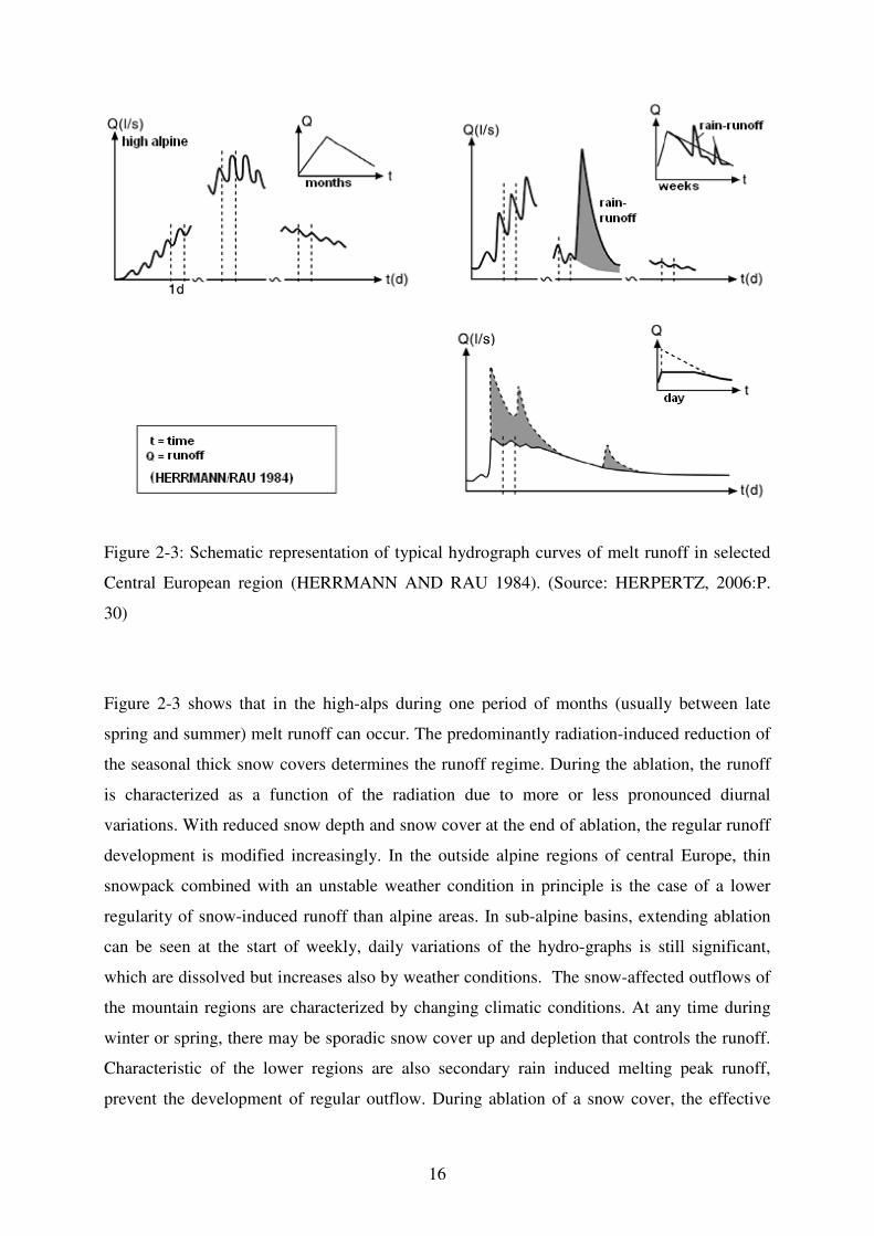
Figure 2-3: Schematic representation of typical hydrograph curves of melt runoff in selected
Central European region (HERRMANN AND RAU 1984). (Source: HERPERTZ, 2006:P.
30)
Figure 2-3 shows that in the high-alps during one period of months (usually between late
spring and summer) melt runoff can occur. The predominantly radiation-induced reduction of
the seasonal thick snow covers determines the runoff regime. During the ablation, the runoff
is characterized as a function of the radiation due to more or less pronounced diurnal
variations. With reduced snow depth and snow cover at the end of ablation, the regular runoff
development is modified increasingly. In the outside alpine regions of central Europe, thin
snowpack combined with an unstable weather condition in principle is the case of a lower
regularity of snow-induced runoff than alpine areas. In sub-alpine basins, extending ablation
can be seen at the start of weekly, daily variations of the hydro-graphs is still significant,
which are dissolved but increases also by weather conditions. The snow-affected outflows of
the mountain regions are characterized by changing climatic conditions. At any time during
winter or spring, there may be sporadic snow cover up and depletion that controls the runoff.
Characteristic of the lower regions are also secondary rain induced melting peak runoff,
prevent the development of regular outflow. During ablation of a snow cover, the effective

17
runoff extends only for a period of days (HERRMANN AND RAU, 1984; BAUMGARTNER
AND LIEBSCHER 1996)
2.5 Snow modelling
Core of snow-hydrological modelling approaches is simulation of snowmelt. The main
processes in snow accumulation and ablation models are: accumulation of new snow, snow
settlement, snowmelt caused by heat transfer from air and rain, water holding capacity,
refreezing of water in the snow pack, temperature changes of snow, and water percolation
through snow. There are two fundamental approaches of snow modelling: the energy balance
method and the temperature index method (TURČAN, 1990).
The energy balance method simulates the physical processes that affect the thermal energy
content of the snow pack such as sensible, latent and ground heat fluxes, heat conduction
between layers, and energy released from phase changes. This type of model requires a
number of inputs including incoming and reflected solar radiation, incoming long wave
radiation, temperature, precipitation, relative humidity, and wind. Normally, data for
determination of long-wave and short-wave radiation balance as well as sensible and latent
heat flows are needed. Because of their nature, physically-based models typically require less
calibration because their parameters are assumed to represent measurable characteristics.
These data are available but limited. As a result, relatively insignificant elements of the
balance are neglected and more important factors like net short wave radiation and albedo as
their determinant are either measured or derived. FERGUSON, (1999) described the
extrapolation of this estimation to be very error-prone. Moreover, BLÖSCHL, (1991)
indicated that temporal and spatial albedo variation strongly varies and is difficult to estimate.
He also described a high sensitivity of the most energy balance procedures for the albedo,
which can lead to much larger misidentifications of the melting volume, for example,
inaccuracies in estimating the air temperature. FERGUSON, (1999) focussed on the high
variability of the particular balance in terms of temporal (daily, seasonal and synoptic scale)
and spatial attributes.
In particular, the energy model approaches usually need very high data, but in the applied
hydrology, preferred temperature index or degree-day factor methods can be used to simulate
snowmelt (BERGSTRÖM, 1975; KUUSISTO, 1980; BRAUN, 1985; WMO 1986;
VEHVILÄINEN, 1992; GRAY AND PROWSE 1993; MARTINEC ET AL., 1994b;

18
RANGO AND MARTINEC, 1995; DUNN AND COLOHAN 1999). Temperature index
methods are based on empirically-derived relationships between air temperatures and melt
rates and require calibration of a number of parameters to represent the regional characteristic
of this relationship. Air temperature is assumed to integrate the effects of advection,
convection, radiation, and latent heat changes on the energy balance of the snowpack (LANG
AND BRAUN, 1990). In this method, snowmelt (�ω) is estimated as a linear function of the
difference between the air temperature (Ta) and a base temperature (Tbase) (DINGMAN,
2002):
�ω = Μ × (Τa − Τ base), Τa ≥ Τ base; Equation 2-7
�ω = 0, Τa < Τ base
Where, M is the melt factor or degree-day factor (DDF). In the traditional temperature index
method, the DDF typically remains constant because the method assumes a constant relative
contribution of all the components of the energy balance.
In basic approach, for determination of the melt volume per time interval, the difference of a
defined limit value of the air temperature and the mean air temperature is formed over a time
step and correlated to a constant melting coefficient. Generally, the procedure is used in the
daily or multi-hourly scale. Therefore, this method can be described for furthest common
snowmelt calculation (BRAUN, 1985; RANGO AND MARTINEC, 1995):
M = a * (T0 – Tlimit) * � t/ 24 Equation 2-8
Where, M is as melt volume [mm/time interval], A is melt coefficient [°C/mm* time interval],
T0 is mean temperature over the defined time interval [°C], T limit is defined limit
temperature for the use (usually 0°) [°C] and ∆t = time interval, to which the melt volume
refers.
The air temperature is the best available meteorological factor, which is to be determined
relatively reliable for area surfaces (BLÖSCHL, 1991). It is also an important influencing

19
factor for all energy balance terms except net radiation. RANGO AND MARTINEC (1995)
showed that temperature-based methods at lower data requirements can provide comparable
good results as energy balance model approaches. Thus, in addition to SRM, the snow module
of HBV model (BERGSTRÖM, 1975; VEHVILÄINEN 1992) and J2000g model
(http://jena.de/jamswiki/index.php/Hydrologcal_Model_J2000g) are based on variants of the
temperature index procedure.
KUHN (1984) considered a constant melt factor during longer periods (days and months), in
which fluctuations of the parameter can be compensated (RANGO AND MARTINEC, 1995).
In the SRM, the melt factor is not a static parameter, but identified as variable time series over
the entire season (MARTINEC ET AL., 1994b). In this way, the change of the sun position
with the season is included into the melt computations. According to VEHVILÄINEN (1992),
the melt factor varies in forest surfaces and opens areas, but time remains constant. GRAY
AND MALE (1981) developed an empirical relation of the melting factor for different slope
angles and exposures. At one index, the ratio of solar radiation received by a slope with a
given inclination and orientation described a horizontal surface.
The temperature index method has been found to be adequate under most circumstances;
however, it cannot account for changes in the surface energy balance caused by diurnal and
annual changes in the incoming solar radiation, albedo, and turbulent energy exchanges
(LANG AND BRAUN, 1990). ANDERSON (1973) gave two basic reasons for using a
temperature index model in operational forecasting: (1) air temperature data are readily
available throughout the all regions in real-time, and (2) tests conducted on two experimental
watersheds showed that the temperature index method (SNOW17) produces results “at least
as good as” those from using the energy-aerodynamic method (HYDRO19). The similar
quality of output between the two models was attributed to the errors involved in determining
input values for the energy method due to the difficulty in measuring the required variables
(ANDERSON, 1973). ANDERSON (1976) showed that the temperature index process
became unreliable when factors other than temperature (such as solar radiation or turbulent
energy exchanges) dominated the melt process. The energy balance model, conversely, gave
good snowmelt estimates for all meteorological conditions in this study.
More recent studies can be found to support either the use of the temperature index method or
the energy balance methods for snowmelt prediction. Arguments for the use of temperature-
based methods continue because of the simple data requirements and comparable performance
to energy balance methods (LANG, 1986; WMO, 1986; KUSTAS ET AL., 1994; RANGO

20
AND MARTINEC, 1995; DALY ET AL., 2000). Reasons for using more complex snow
modelling methods include the increased accuracy of energy balance models at time steps less
than 1 day, appropriateness for modelling spatial processes, the ability to use a variety of
remote sensing observations, and the easy transferability between basins of varying climate
conditions (LANG, 1986; WILLIAMS AND TARBOTON, 1999; STRASSER ET AL., 2002;
SIMPSON ET AL., 2004; WALTER ET AL., 2005). The standard in snow hydrology is that
when only one meteorological variable is available, temperature is the best predictor of
snowmelt (Anderson, 1976). However, regression analysis from ZUZEL AND COX (1975)
showed that when vapour pressure, net radiation, and wind data was available, temperature
was relatively unimportant(Anderson, 1976). But on the other hand, the above mentioned data
can increase the capability of temperature index method in snow hydrological models like
J2000g model.
2.5.1 Snow-hydrological modelling approaches
In many regions of the earth, the melt water discharge from snow covers plays a substantial
role for the water supply and flood development especially in areas with more regular
seasonal snowpack like the alpine or polar area or some mountains located in high latitude
situations. Therefore, a set of modelling tools for the forecast of melt runoff was developed 30
year ago (BERGSTRÖM, 1975; MARTINEC, 1975; WMO 1986; SINGH, 1995). Among the
still most common snow hydrological modelling approaches in the early 70's, MARTINEC
(1975) developed the SRM and the Swedish Meteorological and Hydrological Institute
(SMHI) developed HBV-model for the Alpine region (BERGSTRÖM, 1975; FERGUSON,
1999). Both approaches operate on the daily scale (HBV, shorter time steps) and have a semi-
distributive structure. For other regions, the increasing importance of snow for the winter
runoff dynamics has been identified (HERRMANN AND RAU 1984; BRAUN AND LANG,
1986; RACHNER AND MATTHÄUS, 1986; RACHNER AND SCHNEIDER 1992).
Extensions of the existing approaches and new developments of snow-hydrologic models are
based partially on new scientific realizations (DUNN AND COLOHAN, 1999; FERGUSON,
1999).
Defined objectives, target application space and data availability determine the extent and
structure of snow-hydrologic modelling tools. As in all environmental locations, preferred
modelling approaches, even involving snow-hydrologic modelling components, tried to find a

21
suitable balance between the scientific complexity and a practicable simplicity (FERGUSON,
1999).
2.5.1.1 Conceptual outlines of snow-hydrologic modelling approaches
On one hand, snow-hydrological modelling tells the description of a winter process dynamics
in terms of scientific questions (descriptive approach). Here, usually small-scale process
analyses are the centre of attention, which are to be made possible by deterministic physically
based computation approaches (BLÖSCHL ET AL., 1987; BLÖSCHL AND KIRNBAUER,
1991). On the other hand, predictions of snow water equivalent as well as the temporal
process and the volume of the melting water runoff from snowpack are needed for water-
economical purposes (prescriptive approach). The prescriptive approaches need to be
designed for larger territorial units, such as mesoscale river basins, which require a conceptual
model and technical view of the physical process structure (BRAUN AND LANG 1984;
BRAUN AND LANG 1986; BLÖSCHL ET AL. 1991a). In snow-hydrological modelling, it
distinguished deterministic, conceptual, and also stochastic approaches for the simulation of
complex natural system. In the snow-hydrological modelling, there is distinction between
deterministic, conceptual, and stochastic approaches for the simulation of complex natural
system. When statistical modelling used in conjunction with physically based modelling, it
serves as a valuable tool for addressing important issues (OBLED AND ROSSE, 1977;
VEHVILÄINEN, 1992; FERGUSON, 1999).
In general, hydrologic-snow model approaches accounted for the mass budget and heat flow
of a snow cover. This heat flow is determined either on temperature or on energy-based
methods. The structure of snow routine integrated into the SHE model enables the use of both
the methods. Depending on objective and data availability, methods to be used can be
determined by the user (SINGH, 1995).
The extent of snow-hydrological modelling approaches based primarily on their objectives.
Some models include only the removal of snow, as they were developed as an independent
tool specifically for the prediction of the melting volume and outflow from seasonal snow
cover. Thus, the SRM includes a set of a melting and runoff routine. The accumulation
process itself is not simulated. Rather, measured dataset of snow water equivalent and the
spatial distribution of snow are required as a model input (MARTINEC ET AL., 1994b).

22
SRM model calculates the resulting melt water streams and converts the results together with
the input of rainfall runoff coefficients in daily field outflows. In addition, the effects of
climate changes are involved in applications of the SRM (RANGO 1992, 1995). Other snow-
hydrological modelling approaches are not developed as separate models. It forms a
component of rainfall-runoff and water balance models, and contributes to complete the
system representation. These models include approaches of varying complexity on the
processes of snow accumulation, snow cover and snowmelt (e.g., HBV, HSPF, NASIM,
PRMS / MMS, SHE; WASIM-ETH).
The snow evaporation and sublimation is often considered only in energy-based or detailed
descriptive model approaches, as it is classified as a loss in negligible amount of water
(BRAUN, 1985; DHI 1986; BLÖSCHL AND KIRNBAUER 1991; MARTINEC ET AL.,
1994b; SINGH 1995).
Meteorological data, especially, measurements of air temperature are considered as the
minimum requirement for all snow simulation approaches. Energy based model approaches
require usually at least solar radiation, including albedo data (LEAVESLEY et al. 1983; DHI
1986; BLÖSCHL 1991; SINGH 1995). In addition, often point measured values of the snow
depth or snow water equivalent is required. In order to obtain an approximate spatial
representation, these input data via interpolation and regionalization methods must be
extrapolated at the local area surfaces. The data requirements of the different models often are
based on available regional or national monitoring network of the study area. Especially in the
U.S.A., higher-resolution data are available than in Europe and other countries
(LEAVESLEY, 1989; JAMES, 1991; KUSTAS ET AL., 1994; RANGO, 1996). Switzerland
also has more strongly snow-hydrologic measuring and monitoring networks than other
regions of the Europe (BRAUN, 1985; ROHRER, 1992). In Iran, the collection of snow-
related hydrological data in some parts of Tehran and a few representative mountains close to
some big cities are more intensively operated than another parts of country.
Point measured values of snow parameters are also used to compare the random simulation
results. However, the model calibration must be undertaken in all models by runoff
measurements. First, the spatial-temporal data available from snow parameters is low; on the
other hand, extrapolation of the extremely variable quantities of water equivalent, snow depth
or density on the surface represents a significant failure rate (FERGUSON, 1999). According

23
to KIRNBAUER ET AL. (1994), the combination of modelling with geographic information
systems (GIS) and remote sensing techniques are new possibilities for regionalization and
calibration of snow models (NAKAWO AND HAYAKAWA, 1998). The overall objective,
for example, in newer versions of the SRM by a raster-based remote sensing data coupled
with a direct areal coverage of snow water equivalent and snow distribution. Remote sensing
images can be consulted for the verification of the identified values (RANGO, 1992;
MARTINEC ET AL., 1994b; RANGO AND MARTINEC, 1995). In addition, there are also
opportunities for advanced radar-based determination of rain and snow precipitation, which
require terrestrial measurements (RICHTER, 1995). The practical
application of modern remote sensing and radar techniques is still very limited
to describe. This is mainly due to a low availability of enough temporal-spatial resolution data
and more error recording in snow cover data (RANGO, 1996; NAKAWO AND
HAYAKAWA, 1998; DUNN AND COLOHAN, 1999; LUNDBERG AND THUNEHED,
2000).
2.5.1.2 Spatial differentiation in the snow- hydrological modelling
BLÖSCHL AND KIRNBAUER (1992) considered the area subdivisions and model technical
characteristics in regard to surface area of snow hydrological modelling as an essential
methodological tool (BENGTSSON AND SINGH, 2000). Through the use of available new
technologies (multi-capacity computer, GIS, elevation models, KIRNBAUER ET AL., (1994)
foresee the future of the dawn of a new era in snow hydrological models. Also FERGUSON
(1999) described a trend for distributives modelling, by taking meteorological input data and
different model parameters.
The discretization of the snow-hydrological model approach is based on the usual methods of
general regionalization of hydrological models (e.g., grid, hydrological response units (HRU),
catchment areas, zones, triangulated irregular network (TIN)). Accordingly, the same problem
occurs in the transmission of point values to the surface and the designation of sub-areas of
similar hydrologic response (BLÖSCHL 1996). Most approaches have at least a limited
subdivision of the study areas to reflect the physical heterogeneity of catchments. In
particular, the dominant influence of the ground level to the snow hydrology is determined by
taking levels of terrain into account. Based on the height of the temperature measuring station,
a temperature adjustment amount per level will be carried out, which is considered substantial

24
for snow hydrological simulations (e.g. BERGSTRÖM, 1975; LEAVESLEY ET AL., 1983;
RACHNER AND MATTHÄUS, 1984; BRAUN AND LANG, 1986; BLÖSCHL AND
KIRNBAUER, 1992; MARTINEC ET AL., 1994b; SINGH, 1995; RACHNER ET AL.,
1997). While SRM allowed vertical zoning of any other area subdivisions but, the HBV-
model based on subdivision zones separated simulation of snow dynamics in forest and field
areas (BERGSTRÖM 1975; MARTINEC ET AL., 1994b; FERGUSON, 1999). According to
BENGTSSON AND SINGH (2000) an area division both following topography and landuse
for snow-hydrologic modelling approaches is essential. They described in particularly the
importance of different land covers for the melting dynamics and temporal distribution of
melting induced peak flows. VEHVILÄINEN (1992) reported no distinctions in his
approaches to model the ground level, mainly due to the low relief energy of its test sites in
Finland. However, he highlighted the importance of forests for the snow distribution and
considered the site-specific forest influence by reduction algorithms for the simulation of
accumulation and melt (BERGSTRÖM, 1975; DINGMAN, 1994; POMEROY ET AL.,
1998b). CALDER (1990) represented one of the few model approaches to take in to account
the snow interception (POMEROY ET AL., 1998a).
If the effect of slope exposure and gradient involved in snow hydrological simulations,
its influence can be seen on accumulation and melting process. RACHNER ET AL., (1997)
considered the project SNOW-D is a modification of the terrain height prescribed snow
deposition and distribution as a function of exposure and redistribution of wind. DUNN AND
COLOHAN, (1999) developed a function for the wind-conditional snow redistribution, in
order to determine small-scale snow accumulations, which proved in their Scottish highlands
test areas as significant for the base flow. In many more different approaches, the radiation at
southern and northern slopes in the modelling of the melting process is taken into account
(GRAY AND MALE 1981; LEAVESLEY ET AL., 1983; BRAUN 1985; BLÖSCHL AND
KIRNBAUER 1992). Small-scale topographic factors (valleys, summits and slopes) having
influence on the snow distribution in the modelling in catchment gauges are generally
neglected.
2.5.1.3 Model-technical coverage of the snow accumulation
Regardless of the discretization of the catchment area, the extensive snow accumulation
process in hydrological modelling approaches is derived directly from the rainfall input

25
(BERGSTRÖM, 1975; LEAVESLEY ET AL., 1983; RACHNER AND MATTHÄUS, 1984;
BRAUN, 1985; VEHVILÄINEN, 1992; RACHNER ET AL., 1997). The determination of
precipitation type is of crucial importance in snow modelling. In most models, they used the
temperature in near-surface air layers as a dominant factor which influences the composition
of precipitation at the ground. For determination of the transition of rain to snow, precipitation
is often accepted as simplifying individual temperature threshold value (RACHNER AND
MATTHÄUS, 1984; BRAUN, 1985; VEHVILÄINEN, 1992). In order to involve mixed
precipitation, which occurs frequently, especially in lower layers, LEAVESLEY ET AL.,
(1983) used a temperature interval for the PRMS. At temperatures within the interval limits, it
comes to the creation of mixed precipitation (BERGSTRÖM, 1975). Amount of new or
additional water equivalent of a snow cover is measured finally by amount of area
precipitation fallen in solid or mixed form (BERGSTRÖM, 1975; LEAVESLEY ET AL.,
1983; BRAUN, 1985; VEHVILÄINEN, 1992; RACHNER ET AL., 1997). In other
approaches, for example in SRM, at least point measured values of the water equivalents or
snow depth are required (MARTINEC ET AL., 1994b).
2.6 Snow modelling and water resources
Snowpack act as water reservoirs during the winter months, storing precipitation until spring
and early summer when melt occurs. Water managers rely on this storage effect to better
manage reservoir releases, water deliveries, and water needs throughout the rest of the year
(SINGH AND SINGH, 2001). Snowmelt currently makes up 75% of all the streamflow in
some part of north hemisphere like the west U.S. where surface water resources meet about
90% of the water needs for the regions (FRANZ, 2006).
Figure 2-4: The Long-Term of Snow depth and SWE in Shemshak station, Latyan Catchment
(Data source: Iranian Water Resource Management Company (IWRMCO))

26
Figure 2-5: Anomaly of snow cover extent in North Hemisphere (Source:
http://www.ipcc.ch/pdf/assessment-report/ar4/wg1/ar4-wg1-chapter4, 2007:P.376)
Peak snow accumulation and SWE in the mountains of the Iran can show big variations from
1966-2007(Figure 2-4). Analyses of satellite images snowpack collected over the past decades
indicate that accumulation levels have dropped considerably throughout the high latitude and
mountainous regions and that packs are melting earlier in the year (Figure 2-5) (LEMKE;
REN, ET AL., 2006). Climate impact studies have indicated that even if the most moderate
level of a predicted warming occurs over the next 50 years, snowpack in some regions could
be reduced by up to 60%. This would reduce the spring streamflow volume by an estimated
20-50% (Service, 2004). As the storage effects of snow diminished, there will be less water
available to meet the needs of agriculture, hydropower production, and environmental
protection. The balance between maintaining low flow requirements and maintaining
reservoir storage to meet future water demands will become even more delicate. Because
snow is important as a natural resource and is also extremely variable, accurate estimates of
the volume of water within the snowpack and the rate of release of the water from snow is
required for efficient management (SINGH AND SINGH, 2001).
There is a great deal of uncertainty over whether increased climate variability will cause more
floods, droughts, or significant changes in water supplies (IPCC, 2001). If the changes in the
timing and amount of snow runoff indicated by recent climate studies continue, as well as
continue of growth urban population as a big crisis of 21th Century, accurate hydrologic
predictions will become increasingly important as water managers and hazard response
groups will have to make decision under conditions not previously experienced. It is
necessary that hydrologic predictions systems be able to adapt to and assure reliability in the
face of uncertain future conditions.

27
2.7 Previous Researches in the Latyan catchment
As Tehran is the capital of the country, its water security implies to have a clear vision of the
future. Simulation of the balance of the supply source of the city is very important for
supporting decision makers. Though the hydrological process of Latyan catchment is very
important for water supply and economy of Tehran, the capital of Iran, only few studies have
been carried out so far on the hydrology and water balance of Latyan catchment. Previous
works related to hydrological balance modeling of Latyan catchment are discussed below.
Most important works on precipitation-runoff modeling in Latyan catchment is carried out by
HOSSEIN (1997), FATTAHI (1998), Morid ET AL. (2004) and ZEINIVAND and De
SMEDT(2008). HOSSEIN (1997) analyzed the hydrological behavior of the Roodak sub-
catchment and evaluated the flood simulation by means of HEC-1(Hydrologic Engineering
Center) model. He found that the most runoff in catchment depend on snowmelt during March
to July. Moreover, heterogeneity in rainfall with lack data, seasonal difference snowmelt,
variable channel conditions, inaccurate estimate of routing coefficients and inaccuracy in
hydrological soil groups increased the difference between observed and predicted peakflows,
but finally the differences are not big, therefore HEC-1 model can be used for design of peak
discharge in Roodak and another ungauged catchments. FATTAHI (1998) also used an
Iranian model (SNOW) for analysis and quantification of snowmelt in Latyan dam catchment.
He found that the 64% of all annual precipitation of catchment is snow. He determined the
temperature threshold, and predicted runoff input to the dam during April to June. Moreover,
he noted that in such catchments as Latyan, due to simplicity and data accessible like
temperature, the degree- day method is preferable to predict the snowmelt runoff. MORID
ET AL., (2004) used SWAT (Soil and Water Assessment Tool) for runoff simulation of
Ammameh Sub-catchment of Latyan catchment using different snowmelt algorithm such as
Degree-Day, SRM, and SNOW17. They found better performance of the energy budget
method using synthesized data, compared with solely simple temperature-based method.
ZEINIVAND AND DE SMEDT (2008), modelled snow accumulation and melt using a
distributed hydrological model known as water and energy transfer between soil, plant and
atmosphere (WetSpa) with two different snowmelt simulation modules namely degree day
and energy balance methods for simulating river discharge in the Roodak subcatchment, in
the Latyan dam watershed. They used data of three years of observed daily precipitation, air
temperature, potential evaporation, and wind speed. The discharge data is used for model
calibration. They found that the model performance is satisfactory for both methods with

28
efficiencies of more than 80%. They concluded that the WetSpa model for snow accumulation
and melt has great potentiality to predict the impact of snow accumulation and melt on the
hydrological behaviour of a river basin.
NOURANI ET AL., (2008) and ROSHAN ET AL. (2007) studied the hydrological process in
Ammameh sub-catchment of Latyan. NOURANI ET AL., (2008) developed a
geomorphologic hydrologic model based on distributed flow routing and linear reservoirs
cascade to simulate the runoff of the Ammameh watershed. They proposed that combination
of a non-linear distributed routing model and a linear lumped rainfall-runoff model causes the
proposed model to be a proper runoff routing model. ROSHAN ET AL. (2007) used Smirnov-
Kolmogorov method to optimize the relationship between water and sediment discharge rates
in the Ammameh watershed.
A number of researches related to various hydrological issues to Latyan catchment and water
supply of Tehran can also be found in POURABDULLAH (2006), ZARGHAAMI AND
SALAVITABAR (2006), JAHANI AND REYHANI (2006), GOLTERMAN (2005),
MICAELLI (2007), VALLES ET AL., (1990), KARAMOUZ ET AL., (1999), KARAMOUZ
ET AL., (2001), Bureau of Soil Conservation and Watershed Management (1975),
HYDARIAN (1994), AQIQI (1995), KHOSROSHAHI (1989). Soil Conservation and
Watershed Management (1975) carried out the comprehensive plan of Latyan dam in Latyan
catchment. KHOSROSHAHI (1989) carried out a unit hydrograph study for floods prediction
in Roodak sub-catchment of Latyan. HYDARIAN (1994) evaluates the performance of
different models in predicting soil erosion of Latyan catchment. AQIQI (1995) calculated
depth area duration (DAD) curves in Jajrood area of Latyan catchment for different days.
POURABDULLAH (2006) used RUSLE model, for estimating the amount of erosion Latyan
catchment. The results of modeling showed that the degree of erosion of Latyan catchment
was high because of steep slopes, lack of plant coverage and the quality of soil. VALLES ET
AL., (1990) studied the soil alkalinization and salinization in some parts of Latyan catchment.
A system approach to water resources management of Latyan catchment is discussed by
KARAMOUZ ET AL., (1999). ZARGHAAMI AND SALAVITABAR (2006) used system
dynamics which considered the water supply sources, demand sources (as domestic, irrigation
and industry uses) and management tools (demand reduction, inter-basin water transfer) for

29
urban water management of Tehran. They predicted water shortage in the future years in the
capital of Iran. KARAMOUZ ET AL., (2001) used a system approach to water resources
development in Tehran considering its complex system of water supply and demands.

30
3. METHODICAL APPROACH

31
3.1 Hydrological System Analysis and Delineation of Hydrological
Response Units
3.1.1 Hydrological System Analysis
The hydrological system analysis is the base for the delineation of the Hydrological response
units (HRUs) and the calibration of the spatially distributed conceptual hydrological model
J2000g. Initially, the hydrological system analysis studies the interactions of the landscape
parameters soil, water, vegetation and climate in order to understand the system response to
rainfall and therefore the generation of the respective hydrological response. Also, the
examination of the hydro-meteorological time series using data analysis methods for changes
in hydrological system response is an important preparation for the rainfall-runoff modeling
of the catchment.
3.1.1.1 Data Analysis of Hydro-Climatological Time Series
The quality of the model output is directly depending on the input data (BEVEN, 2001).
Hydrological models are driven, in part, by hydrometeorological data, which contains hourly,
daily, or monthly field observations. The resulting time series are never perfect and the data
contains data errors (BEVEN, 2001). The data errors are divided into systematic errors and
random errors. The first group contains errors which affect the measuring instrument
systematically (BEVEN, 2001) and result in a constant measurement bias. These errors can be
caused, for instance, by false calibration of the instrument. Random errors, on the other hand,
are caused by randomly occurring factors, such as interference of the automatic recording by
animals. To achieve good modeling results it is crucial to control for data quality.
• Rainfall Data
Rainfall data are measured as point observations and there are several potential sources of
data errors associated with those measurements (DINGMAN, 2002:P.114). The design of rain
gauges can lead to a standard error between 3 to 30 % of the total annual measured rainfall
sum (DINGMAN, 2002:P.115). These data errors can be corrected using an approach
presented by RICHTER (1995). Rainfall time series might also include missing values. Here,

32
DINGMAN (2002:P.115-117) suggests the following methods for data filling: station average
method, normal ratio method, inverse distance weighting, regression analysis or the most
common technique: the double mass curve between two stations.
• Runoff Data
The discharge observed at the runoff station is an integrated value over the entire catchment.
In a hydrological model, the data is used for calibration of simulated runoff against observed
runoff. Therefore, it is necessary to check runoff data for homogeneity and inconsistency
(BEVEN, 2001). The most common technique, in case of available data at a nearby station, is
the double mass curve (BEVEN, 2001). The double mass analysis compares two
neighbouring measuring stations by the plotting of accumulated volumes. Changes in the
runoff records will be visible in slope changes compared to the reference line.
This analysis gives information on missing values or changes in the catchment affecting the
measured runoff. The resulting data was used to compute the annual and monthly average
runoff and to establish the rainfall runoff relationship.
• Additional Datasets
The time series data on wind speed, humidity, and temperature as well as snow depth and
snow water equivalent (SWE) time series was checked for homogeneity and consistence using
the aforesaid methods for rainfall and runoff data analysis. Missing values were filled by
using regression analysis.
3.1.1.2 Spatial Data Modelling
Hydrological models require spatial information of the hydrometeorological information. The
hydro-meteorological time series used, however, contain measurements at point scale. For a
spatial representation of these parameters the missing information has to be interpolated.
Here, several methods exist such as Thiessen Polygons, linear regression and inverse distance
weighting (IDW) (WACKERNAGEL, 1995; KITANIDIS, 1997; WEBSTER AND OLIVER,
2001).
The regionalization of the hydro-meteorological datasets is used for the transfer of punctual
values to the model units. The procedure was taken from the hydrological Model J2000

33
without any changes and is based on the inverse distance weighting (IDW) approach. The
regionalization consists of several steps (KRAUSE, 2001; JAMSWIKI, 2010): First, the linear
regression is applied to determine the relationship between station measurements and the
respective station elevation. In the second step, the numbers of stations next to each HRU is
determined, whereas the user defines the number of stations necessary to take into account.
Then the distance between the found stations and each HRU is computed. To account for the
difference in the distance between HRU and station, the application of a user defined
weighting factor weightings the distances. In the third step, the final weighting factor for the
hydrometric station is computed applying an inverse distance weighting method (. In the last
step, the actual data values were calculated under consideration of the weighted values of
stage 3 and the elevation factors of stage 1. For more detailed information on the
regionalization algorithm in J2000g refer to JAMS (http://jams.uni-
jena.de/jamswiki/index.php/J2000g) and KRAUSE (2001).
Another important stage in this framework is to check the spatial data for missing values.
Particularly important is the digital elevation model (DEM), which is one of the most
important datasets, because it will be used for the delineation of the stream network,
catchment boundaries and topographic parameters such as slope, aspect, flow direction and
flow accumulation. The DEM can be derived from remote sensing imagery, such as synthetic
aperture radar (SAR) Interferometry (LUDWIG, HELLWICH ET AL., 2000) or from the
Shuttle Radar Topography Mission (SRTM) (U.S. GEOLOGICAL SURVEY EROS DATA
CENTER AND NASA, 2007). The SRTM-DEM, especially, often contains voids, which
have to be filled for a hydrological application (KÄÄB, 2005; GROHMAN ET AL., 2006;
WOLF, 2009).
3.1.2 Delineation of Hydrological Response Units
The relationship between rainfall-runoff of a catchment is determined by the following a wide
variety characteristics: geology, topography, land use, soils, climate and vegetation cover
(BEVEN, 2001:P.179). To account for a realistic representation of the catchment
characteristics, the model used should be fully distributed. This type of model is difficult to
apply because the model needs high spatially distributed input information of the landscape
parameters, which cannot be measured at the requested resolution (BEVEN, 2001;
BLÖSCHL, 2005). Therefore, the attempt has been made to define model entities that show a

34
“hydrological similarity” (BEVEN, 2001:P.179), which can be defined using one of the
following three approaches. The first, the concept of Aggregated Simulation Area (ASA) has
been applied in the SLURP (Semi-distributed Land Use-based Runoff Processes) model
(KITE, 1995). This concept involves aggregating simulation areas which are heterogeneous in
their land cover and elevation; however, the distribution of these parameters within the
respective entity is known. These ASAs have the requirement of contributing runoff to a
stream channel and, therefore, act as sub catchments (KITE, 1995). The second approach, the
Representative Elementary Area (REA) (WOOD, ET AL., 1990) defines minimal areas in
which the spatial heterogeneity of hydrological variables such as infiltration, evaporation, and
runoff are unimportant. The distribution of these variables within the areas is represented by a
probability function. The third concept, the Hydrological Response Unit (HRU), was
introduced by LEAVESLEY, LICHTY ET AL. (1983) as model entities in the Precipitation
Runoff Modelling System (PRMS). HRUs are characterized as homogenous areas with
respect to their hydrological response (LEAVESLEY ET AL., 1983:P.9). This approach was
extent by FLÜGEL (1995, 1996) who defined HRUs as areas with common in “climate, land
use and underlying pedo-topo-geological associations controlling their hydrological
dynamics” (FLÜGEL, 1995:P.426). The delineation of HRUs involves the definition of
classification criteria, which are based on hydrological system analysis (FLÜGEL, 2000). The
concept of HRUs has been tested and applied in several studies as an integrated
regionalization tool (BONGARTZ, 2001; KRAUSE, 2001; KRAUSE, 2002; SCHEFFLER
ET AL., 2007; SCHEFFLER 2008, KRAUSE AND HANISCH., 2009).
It can be concluded that the concepts of HRUs are the only modeling entities that consider all
landscape parameters important in hydrological processes. Therefore, the HRU-approach has
been applied in this study and is explained in the following section.
3.1.2.1 Concept Approach of Hydrological Response Units
The HRU concept, according to FLÜGEL (1995; 1996), is based on the representation of the
catchment heterogeneity in the form of entities showing a similar or equal system response.
The climate and other landscape parameters of geology, soil, and vegetation are strongly
interacting to each other. The natural vegetation depends on climate, relief and soil type. The
soil is formed from bedrock material through various weathering and erosion processes.

35
Climate conditions determine the intensity of these various processes and, therefore, the types
of soil formed. Distribution and formation of soil is also determined by the topography
controlling the accumulation of soil material and the water movement within and on top of the
soil column. A specific combination of geology, soil, relief, vegetation and climate
characteristics, therefore, generates a specific system response (SCHEFFLER, 2008).
The HRUs divide the catchment into areas with similar or equal geology, soil-relief-
vegetation and climate combinations. These entities are delineated based on detailed
hydrological system analyses in a Geographical Information System (GIS) (FLÜGEL, 1995;
1996). The general object of using HRUs is to reduce the data inside each grid cell to unit
information per layer. That means after applying this discretisation inside each grid cell, just
one value for each landuse, soil, geology, slope, aspect, etc. exists. Based on the results of the
hydrological system analysis the GIS datasets are reclassified, aggregated and overlaid in a
step-by-step procedure. These entities act as model input for the rainfall-runoff simulation of
the study area.
3.2 Water Balance and snowmelt-Runoff Modelling with J2000g Model
To obtain the above stated study goal, the snowmelt contains in the catchment has to be
estimated. Due to importance of snowmelt-runoff in the catchment, spatial distribution of the
SWE and snowmelt is simulated. For this purpose, the spatially distributed conceptual
hydrological model has been applied. The delineated HRUs serve as spatial modelling entities
in the model. The following section gives an introduction in the model design but also the
steps of the modeling process such as preparation of input data (Section 3.2.2),
parameterization and calibration (Section 3.2.3) are described.
3.2.1 The Structure of Modelling System of the J2000G Model
The model used for this study was the spatially distributed conceptual hydrological model
J2000g model, which was adapted from the J2000 model (KRAUSE, 2001; KRAUSE, 2002)
within the Modelling framework system JAMS (KRALISCH AND KRAUSE, 2006). The
structure of the model is shown in Figure3-1. The model has been successfully applied in
catchments of between 100 to 16000 km² in Thuringia, Germany for impact of climate change

36
(KRAUSE and HANISCH, 2009). Additionally the model was applied successfully in the
Nam Co basin (about 20,000 km ²) in Tibet (KRAUSE ET AL., 2010 in review). The other
version of implemented models like, J2000 and J2000s successfully applied in various spatial
scale and area ranges from basic scientific investigations in small catchments in Germany (2 -
13 km ²), and in the processing of basic and applied research in mesoscale (about 50-1000 km
²) catchment Germany, South Africa, Tasmania and the USA to macroscale modelling in the
headwaters of the Brahmaputra (about 500 000 km ²) under the Brahmatwinn project
(KRAUSE, 2001; BÄSE ET AL., 2006;SCHEFFLER ET AL., 2007; SCHEFFLER, 2008;
KRAUSE ET AL., 2009; http://www.brahmatwinn.uni-jena.de).
Input data:P,Tmin,Tavg,Tmax,WS,...
Data Regionalization
Additionaldata:Radiation calculate,...
Snow Module
Soilwater module
Direct Runoff
GW Retention
Direct Runoff
DR Retention
Baseflow
Percolation
Total Runoff catchment
Act. Et
Pot. Et
Figure 3-1: The Concept of Modelling System of the J2000g Model
As shown in the figure, the modelling system is divided into process modules such as the
snow, soil water, and ground water recharge modules.
For each modelling unit (HRU), in the snow module, rainfall is computed as snow or rain
based on temperature and precipitation input and degree day factor. Then the surface runoff
and subsurface runoff are calculated in the soil module, but because the J2000g model is
defined as simplified model, the surface runoff and subsurface runoff computed together as

37
direct runoff. In addition, base flow components are calculated in the groundwater recharge
module. Afterwards, the simulated values of all the runoff components are added to the
respective storages. This process is repeated until the water is transported to the catchment
outlet.
The 2000g was developed for historical simulations as well as for snow hydrological
modelling. The development was guided by the following requirements: (1) continuous and
distributed simulation of important hydrologic characteristics in monthly time steps; (2)
applicability of the model to the Iranian mesosclee catchments (Latyan, 700 km²); (3) process
oriented and spatially distributed modelling; and (4) robust predictive ability with a small
number of calibration parameters in areas with poor data.
The model J2000g requires spatially distributed information related to topography, landuse,
soil type and hydrogeology to estimate specific attribute values for each modelling unit. A
modelling unit can be a raster cell, a process unit, or a subbasin provided that spatial
information is available for each attribute within each unit. J2000g also requires
meteorological inputs (precipitation; minimum, average and maximum temperature; sunshine
duration; wind speed and relative humidity) from one or more observation stations. The
measured point data are transferred to each model unit using the spatial interpolation approach
available in J2000 which is a combination of an optional elevation correction and an inverse-
distance-weighting (IDW) interpolation. The elevation correction is made when the degree of
correlation (calculated with a linear regression for each time step) between the variable values
and the respective station elevation shows a coefficient of determination (r2) of equal or
greater 0.7. In this case, the specific elevation dependent lapse rate, calculated from the
regression, is used for the further processing along with IDW. If the r2 is smaller than 0.7 then
only IDW is used. Next, net radiation (needed within the potential evapotranspiration (PET)
module) is calculated from climate input data using the methods presented in ALLEN ET
AL., (1998). Then potential evapotranspiration (PET) is computed according to the Penman-
Monteith approach for various vegetation and land-use types (JAMS WIKI, 2010).
Snow accumulation and snowmelt are simulated with a simple approach that estimates snow
accumulation is related on a base temperature (Tbase) and snowmelt with a time-degree-
factor (TMF). During time periods when air temperature is above Tbase, precipitation and
snow melt is transferred to the soil-water module. This module consists of simple water
storage with a capacity defined from the field capacity of the specific soil type within the
respective modelling unit. For calibration purposes, the entire distribution of storage capacity

38
values for all modelling units can be shifted up or down with a multiplier (FCA) that has the
same value for all modelling entities. Water stored in the soil-water storage can only be taken
out through evapotranspiration. The actual evapotranspiration (AET) is determined by the
saturation of the soil water storage, the potential evapotranspiration and a calibration
coefficient ETR. The ETR coefficient controls when potential evapotranspiration is reduced
due to limited water availability. Runoff is generated only when the soil-water storage reaches
saturation. The partitioning of generated runoff into direct runoff and percolation is based on
the slope of the modelling unit and a calibration factor LVD. The percolation component is
transferred to a groundwater storage component; outflow from this storage is simulated using
a linear outflow routine in order to calculate baseflow with the help of a recession parameter
GWK. The total runoff at the outlet of a catchment results from the summation of the direct
runoff and the baseflow components from each modelling unit. The primary purpose of the
J2000g model is to provide spatially distributed long-term estimates of the amount and
seasonal distribution of the following hydrological quantities: actual evapotranspiration,
runoff generation, and groundwater recharge. In the J2000g model, streamflow is computed
by simply summing up the runoff components generated in each modelling unit of the
catchment. Because of these simplifications, the model cannot account for losses and
transformations during runoff concentration or for specific hydrological conditions such as
streamflow and groundwater losses in karst regions or the influence of human activities
KRAUSE AND HANISCH, 2009).
3.2.1.1 The Snow Module of the J2000g
In the snow module, snow cover computation is implemented as simple accumulation and
snowmelt approach. The method decides on the basis of the air temperature whether water is
saved as snow on a model unit or potentially existing snow melts and produces snowmelt
runoff. For this purpose, two temperatures are calculated from the minimum temperature
(Tmin), average temperature (Tavg) and maximum temperature (Tmax), which is given
below:
The accumulation temperature as:
min( ) / 2acc avg
T T T= + [°C] Equation 3-1
39
And,the snowmelt temperature as:
max( ) / 2melt avg
T T T= + [°C] Equation 3-2
If the accumulation temperature (Tacc) lies on or below a threshold (Tbase) value that needs
to be given by the user, it is assumed that potentially occurring precipitation falls as snow. It
is then saved on the model unit. If the snowmelt temperature goes beyond the temperature
threshold Tbase, the snowmelt is calculated with the help of a simple snowmelt factor (TMF).
Therefore, a potential snowmelt rate is calculated on the basis of the TMF (in mm/d K), the
temperature threshold and the snowmelt temperature as shown below:
( )p melt base
SM TMF T T= −� [mm/d] Equation 3-3
This potential snowmelt rate is then compared to the actual saved snow water equivalent
which is then partly or fully melted. The resulting snowmelt water is passed on as input to the
following module.
A more detailed description of the snow module can be found in (http://jams.uni-
jena.de/jamswiki/index.php/Hydrological_Model_J2000g) and KRAUSE (2001).
3.2.2 Preparation of Input Data
The model J2000g requires the following data files. Also after developing model for the
SWE; a new snow water equivalent data is added as input data files that, shown in the
following table.

40
Table 3-1:Input Data files of J2000g Model
DESCRIPTION UNITS
Absolute Humidity g/cm³
Relative Humidity %
Observed Runoff m³/m
Observed Rainfall mm
Observed Snow Water Equivalent(SWE)* mm
Sunshine Duration H
Maximum Monthly Temperature °C
Minimum Monthly Temperature °C
Mean Monthly Temperature °C
Wind Speed m
The needed monthly mean temperature for some stations was not provided, therefore it was
computed as the average of the maximum (Tmax) and minimum (Tmin) monthly temperature.
Also, the model requires the absolute humidity as an input parameter dataset. The dataset,
hence, has been calculated in several steps, depicted in the following equations:
1. Computation of the saturation vapor pressure es (DINGMAN, 2002:P.586)
17.3*
237.3( ) 6.1078 *T
Tse T e += Equation 3-4
2. Computation of the maximum humidity with T as mean air temperature and the computed
values for es
216.7( ) *
273.15m sR T e
T=
+ Equation 3-5
3. Computation of the absolute humidity (Ra) by taking relative humidity Ru and maximum
humidity Rm into account.

41
( ) *100
ua m
RR T R=
Equation 3-6
All input data files (Table 3-1) were transformed into ASCII- format. In addition to the actual
data values, J2000g requires information on geographical location as well as the elevation of
the station. The geographical location for the stations was derived using Arc GIS 9.3 (ESRI,
2008). In case of missing elevation data, that information was taken from the available digital
elevation model (SRTM 2007).
3.2.3 Parameterization and Calibration
The model J2000g requires parameter input files in order to describe the natural
characteristics. These parameter values were obtained from literature and are described in
Section3.2.1. Additionally, the model J2000g contains direct model parameters: 1 parameters
in the groundwater recharge, 4 parameters in the soil module, and 2 snow module parameters,
shown in Appendix A.
The goal of model calibration is a satisfactory fit between simulated and observed variables
(REFSGAARD AND STORM, 1996:P.42). Therefore these parameters have to be adjusted.
That is necessary for three reasons as stated in BLÖSCHL (2005): First, the hydrological
models are based on empirical equations which are depended on basin properties. Second,
model boundaries are mostly poorly defined. The model calibration adjusts input errors such
as measurement errors. Third, landscape parameters such as soil, vegetation, geology and
topography are highly variable in space, and the knowledge of their real occurrences as well
as physical properties is limited. Here, parameter adjustment accounts for unknown
parameters and characteristics (SCHEFFLER, 2008).
According to REFSGAARD AND STORM (1996), three approaches can be used to calibrate
hydrological models: 1) manual adjustment using “trial and error”, 2) automatic model
calibration, and 3) a combination of 1) and 2). The “trial and error” method requires expert
knowledge about the model structure and involves a lot of time because the manual

42
assessment it needs a larger number of model runs (REFSGAARD AND STORM,
1996:P.47). The automatic model calibration, however, is much faster and less subjective than
the manual method (REFSGAARD AND STORM, 1996:P.47). The drawback of the
automatic parameter adjustment is the evaluation of the model fit depending only on the
objective function, which can lead to a wrong model solution. In order to account for the
catchment characteristics and decrease the time effort, a combination of both methods is
recommended (REFSGAARD AND STORM, 1996:P.48). In this study, the automatic
parameter adjustment was used to define sensitive parameters and parameter ranges.
3.2.3.1 Automatic Parameter Estimation using Sensitivity Analysis
Sensitivity analysis is a significant tool in hydrological modelling. Particularly during the
model design and model calibration, sensitivity analysis provides a better understanding of the
relationship between model parameters and model processes (MCCUEN, 1973). It allows the
identification of sensitive parameters influencing the model output (BAHREMAND AND DE
SMEDT, 2008:P.2).
KRAUSE (2010) estimated the parameter sensitivity in J2000g using various methods like
single and the multi parameter Monte Carlo Analysis in the mesoscale catchment (BODE),
Germany. The author reported that in single parameter approach the seven model parameters
(LVD, GWK, Tbase, TMF, FCA, and ETR) some of the parameters particularly two snow
parameters (Tbase and TMF) have influence on the model results only in part of the year
whereas others are active all the time, but heir impact was quantified as medium to low for the
overall period. KRAUSE (2010) also found that in the temporal domain, by looking at runoff
ensembles, Tbase had some higher impact in the middle of the time series, but two parameters
LVD and GWK had the larger impact on the all of time series and model results. A more
detailed description can be found in KRAUSE (2010).
For the parameter sensitivity estimations and their ranges in the Latyan catchment, single and
the multi parameter Monte Carlo Analysis method in the monthly model of J2000g has been
applied. Here, first, the analysis of the results was made by visual inspection of parameter
values versus single efficiency criteria. Additionally the analysis of the multi-parameter
estimation was done by visual inspection of ‘dotty-plots’ and more analytical method
described in KRAUSE, (2010). This method was based on 10000 Monte-Carlo runs computed
with the parameter ranges shown in table 3-2.

43
Table 3-2: J2000g parameters and feasible parameter range for monthly
Name Process Range(monthly) Unit
Tbase Snow -10 - 0 C
TMF Snow 0 - 20 mm/K
FCA Soil water 1 - 20 -
ETR Soil water 0 - 1 -
LVD Soil water 0 - 50 -
DQK dQ retention 1 -
GWK bQ retention 0 - 10 -
Reactions were then evaluated using four objective functions: Nash-Sutcliffe-Efficiency
(NSE) (NASH AND SUTCLIFFE, 1970), logarithmic Nash Sutcliffe Efficiency (log. NSE),
relative percentage volume error (pbias) and the coefficient of determination (R²).
• Nash- Sutcliffe Efficiency
The Nash-Sutcliffe Efficiency (NSE) is the model coefficient of efficiency (Nash and
Sutcliffe, 1970), which expresses the fraction of the measured streamflow variance that is
reproduced by the model. The NaS is calculated as follows:
2
1
2
1
(( ) ( ) )
1
(( ) ( ) )
n
obs i sim i
i
n
obs i iobs
i
Q Q
NSE
Q Q
=
=
−
= −
−
∑
∑ Equation 3-7
With Qobs representing the observed runoff value and Qsim the modeled runoff value at time
i, obs Q defines the observed mean runoff for the given time period. The range of the NSE
lies between −∞ and 1; a NSE of 1, hence, confirms a perfect fit. As stated in KRAUSE,
BOYLE ET AL. (2005:P.90), the disadvantage of the NSE is an insensitivity to model over
and under predictions, especially in periods of low flow. The authors suggested using the NSE
with logarithmic values.
• Logarithmic Nash Sutcliffe Efficiency

44
The calculation of the logarithmic Nash-Sutcliffe Efficiency (log. NSE) is carried out as
follows:
2
1
2
1
(( ) ( ) )
log. 1
(( ) ( ) )
n
obs i sim i
i
n
obs i iobs
i
Q Q
NSE
Q Q
=
=
−
= −
−
∑
∑ Equation 3-8
The influence of the low flow values is stronger than in the NSE calculation due to the
logarithmic values of obs Q, Qobs and Qsim. This leads to a higher sensitivity to over and
under estimation of the observed runoff during low flow conditions (KRAUSE, BOYLE ET
AL., 2005:P.91).
• Relative percentage volume error
The percent bias (Pbias) is a measure of the average tendency of the modeled flows to be
larger or smaller than their observed values. The optimal PBIAS value is 0.0; a positive value
indicates a model bias toward underestimation, whereas a negative value indicates a bias
toward overestimation (GUPTA ET AL., 1999). PBIAS is expressed as:
, ,1
,1
( )(100)
( )
n
i obs i sim
i
n
i obs
i
Q Q
PBIAS
Q
=
=
−
=
∑
∑ Equation 3-9
Pbias is deviation of streamflow discharge, expressed as a percent, Qi,obs is observed stream
flow and Qi,sim is simulated streamflow .
• Coefficient of determination r ²
The coefficient of determination r ² is defined as the squared value of the coefficient of
correlation according to Bravais - Pearson. It is calculated as:
2
2 1
2 2
1 1
( )( )
( ) ( )
n
i i
i
n n
i i
i i
O O P P
r
O O P P
=
= =
− −
=
− −
∑
∑ ∑ Equation 3-10
With O observed and P predicted values.

45
R ² estimates the combined dispersion against the single dispersion of the observed and
predicted series. The range of r² lies between 0 and 1 which describes how much of the
observed dispersion is explained by the prediction. A value of zero means no correlation at all
whereas a value of 1 means that the dispersion of the prediction is equal to that of the
observation.
The vital identification of a well fit between the two outputs was the visual comparison of the
observed and simulated runoff. In the second step, the “Automatic” method was used to
determine final parameter values which acted as baseline values for the estimation of
uncertainty.

46
4. STUDY AREA AND DATA BASE

47
The case study chosen is located in semi-arid mountainous region. Snow and snowmelt is a
vital source of water supply system. This catchment is one of the most important source of
water supply for population about 13 million. Hence prediction of snowmelt can be help to
water resource management and developing of water supply system. Unfortunately data base
of catchment is not proper and access to various data, especially hydro-meteorological data,
except temperature, is complex due to spatial variability and complex topography. Therefore
one spatial distributed hydrological model based on availability of data was used for
hydrological snow modelling to development of water resource management of area.
The Latyan catchment covering an area approximately 700 km² is located in about 35 km of
north-eastern Tehran (capital of Iran), between Latitudes 35°, 45’ to 36°, 50’ N and longitudes
51°, 23’ to 51°, 51’ E. Figure 4-1 shows the situation of the catchment.
Figure 4-1: Geographical Location of the Latyan catchment

48
The Latyan catchment is located in a mountainous area, and very steep slopes. Elevation
difference between the highest and lowest point is about 2825 meters, with the highest point
about 4325m.a.s.l at the Valdarbaldar Mountain and the lowest point, at the Latyan dam
outlet, about 1500 m.a.s.l..
The main river of this catchment is Jajrood River. North side includes 3 main tributary
streams like Garmabdar, Shemshak and Ahar, and joint together with Fasham and Oushan
then also in the middle of catchment, Ammameh River and tributary streams of Roodak-
Qhuchak joint and then drains in to Lake of Latyan dam. Moreover, in the Eastern part of
catchment, streams of Kond, Afjeh, Bargjahan, and Lawasan(north and south Lewarak) with
amounts of small tributaries directly drains in to lake dam.
The Latyan dam is one of the primary sources of water supply for the Tehran metropolitan
area, with its over 13 million people. From 1988, due to increasing water supply demand of
Tehran, yearly about 140 MCM water is transferred to Latyan dam via tunnel from Lar River
to Latyan dam. Therefore this extending and transfer water increases the annual volume
capability regulation of water dam to 410MCM annually. In addition to its importance for
municipal water use, runoff from the Latyan also provides water for agriculture (over 70000
hectares in downstream) and for hydropower generation (45 Megawatt). Besides, this dam,
the primary water management structure in the basin, provides water over 95 MCM of storage
(http://www.tw.org.ir/dams/selectdam_en.asp).
Figure of 4-2 illustrates the streams and drainage network of Latyan dam catchment.

49
Figure 4-2: Streams and Network and Subcatchments of the Latyan Catchment
4.1 Study Area
4.1.1 Climatic Condition
The Latyan catchment is influenced by Mediterranean and Polar air masses. Distribution of
rainfall that belongs to both systems is 27, 39, 30 and 4 for autumn, winter, spring and
summer respectively. This distribution rainfall system comparison to distribution of rainfall in
Latyan catchment namely 26, 38, 32 and 4 from autumn to summer has very low difference.
The characteristic of these air masses is high rainfall in winter and one dry season that
continue between 3 to 5 months (WEI, 2004).
Generally can be see an important relationship between rainfall and altitude, namely by
increase of altitude, rainfall increase. Normally above 3000 m, rainfall changes to snow.

50
According to Iranian Water Framework(JAMAB) relation between variability of rainfall to
altitude, with due attention to 25 year average of rainfall in 12 rainfall measurement stations
Latyan dam catchments is described below:
P = -162.8+0.376Z that, Equation 3-11
P= annual average precipitation (mm)
Z= altitude of station (m)
According to this function, variability of rainfall to elevation of each 100-meter increase is
37.6mm and correlation coefficient between annual average precipitation and elevation is
0.985(MAHMUDIAN:P.82, 2002). According to Water and Energy Institute(WEI), 2004)
reports, based on coefficient correlation between geographical latitude and amount of
precipitation at measuring stations of Latyan catchments, variability of rainfall is 10mm.
From elevations above 3000 m.a.s.l precipitation form, fallen as snow. After determination of
average annual precipitations procedure, average annual precipitation of Latyan catchment is
about 573mm.The estimated annual rainfall in Latyan catchment is 406.7 MCM. Minimum of
annual rainfall is belong to Qhuchak station with 245mm and annual maximum of rainfall
belong to Garmabdar station with 756mm. Out of 39 percent of winter precipitation, about
35% is snowfall that fallen over limestones of high altitude of catchment and make different
avalanche forms in tributaries of Shemshak, Ammameh, Laloon, Ahar, and Garmabdar(WEI,
2004). The figure 4-3 shows 40 year mean monthly precipitation in Roodak and Latyan
stations. Most of Latyan's precipitation is in winter. It falls at low elevations as rain (winter
discharge) and at high elevations as snow, which produces spring discharge as it melts. At
intermediate elevations, discharge is a mixture of the two seasons. The maximum of temporal
precipitation occur in March and April about 87 and 72 mm for Roodak and Latyan
respectively. Additionally minimum of precipitation is occurred in summer especially
between August to September about 6 and 3.5 mm for Roodak and Latyan stations.

51
0
10
20
30
40
50
60
70
80
90
100
Oct. Nov. Dec. Jan. Feb. Mar. Apr. May Jun. Jul. Aug. Sep.
mean
mo
nth
ly p
recip
. m
m/d
Roodak
Latyan Dam
Figure4-3: Mean Annual (1967-2007) Monthly Precipitation in the Latyan Catchment(Latyan and Roodak Station)
-10
-5
0
5
10
15
20
25
30
35
40
Oct Nov Dec Jan Feb Mar Apr May Jun Jul Aug Sep
mean
mo
nth
ly t
em
p. °C
avg
min
max
Figure 4-4: Mean Annual (1967-2007) Monthly Precipitation in the Latyan Catchment (Latyan Station)
Generally temperature in months between end of December to middle March fall to below
0°C and this time all the rainfalls fall as snow. Again after March temperature increase to
above 0°C and snowmelt start in this time and increasing of temperature will continue and in
end of July and August reach to above 30°C (Figure 4-4). Maximum of mean annual
temperature of catchment belong to Latyan station with 14 °C and minimum of mean annual
temperature with 7 °C belong to Rahatabad station. The absolute minimum temperature
belongs to Kamarkhani station is -32°C and absolute maximum of temperature is +38°C in

52
Latyan station. The mean frozen days is about 75 day and mean dry days are reported about
120 days. According to Amberjeh procedure, can be seen 3 types of climates in Latyan
catchment: high elevations, sub humid cold and semi-arid (WEI, 2004).
4.1.2 Geomorphology
4.1.2.1 Slope
The latyan catchment is one of Iranian mountainous catchments and its elevation varies from
1500 meter above see level (m.a.s.l) in Lake Dam to 4300 m.a.s.l in summits. Maximum
elevation in this catchment is 4325 m.a.s.l in the Volderbalder Mountain and minimum is
1500 m.a.s.l in outlet of Latyan dam. This catchment is surrounded by Lar dam basin from the
north, North Tehran basin from the south, Damavand basin from east and by Karaj basin from
west. Base on Hypsometric maps, more than elevations of this catchment are located between
2300-2800 m.a.s.l that is 34% of area catchment. The extent of 44 km² of lands catchment is
plateaus and gorge upon alluvial deposits. About 170 km² are geomorphologic unit of hills
and 486 km² are mountainous units. Based on gradient maps of Latyan, more than 90% of
catchment has gradients above 15% and the higher gradient of catchment located in class of
30-50%. Gradient of above 50% is about 25 percent of all area Latyan catchment. Figure 4-5
shows the slope map of Latyan catchment.

53
Figure 4-5: Slope Classes in the Latyan Catchment
4.1.2.2 Aspect
Low gradient lands mainly located in south catchment which is around Lake Dam and main
tributaries, and high gradient lands are located in limestone elevations of northern catchment.
Most of gradient surface (face) is located to direct of south with 33.7% and then with 20% to
direct of north. Figure 4-6 illustrates the exposition condition of Latyan catchment.

54
Figure 4-6: exposition condition of the Latyan Catchment
4.1.3 Landcover/Landuse
The land use map for this study with 90 m grid size, showing the land cover for 2005-2006, is
depicted in Figure 4-7. The map shows 5 different types of land cover: 81% of the basin is
covered by deciduous shrubs, 6% by deciduous broad trees, 2% by short grass, and about
11.0% by agriculture and settlements.

55
Figure 4-7: Landcover/Landuse of the Latyan Catchment
4.1.4 Geology
The geological characteristic of the Latyan catchment is very complex and is located between
zones four and five of the Alborz geological unity and on the middle part of central Alborz
Mountains. Therefore, different geological formations from oldest (early Cambrian) to the
youngest (Quaternaries sediments) can be found.
In stratigraphy of Latyan catchment, formations of Paleozoic, Mesozoic and Cenozoic has
seen. Cambrian, Hiatus of Ordovician, Silurian, Upper Cretaceous, Paleocene and Neocene
activities can be seen in the catchment (WEI, 2004, P: 10)
Generally, the northern and central region of the Latyan basin is older than other parts. In this
part, different types of tuff (shaly, calcareous and soft), dolomite, limestone, thin layers of

56
sandstone, sandy marl, silt, as well as basaltic-andesitic lava flows and volcanic intrusive
screes can be found. In addition, due to mountainous location of catchment, Quaternary
activities was limited, but these sediments due to erosion of older formations in long terms
deposited in the boarder of the main rivers like Meygoon and Kond River and other tributaries
of catchment, especially in the supreme of Latyan lake dam. This part of the catchment is
characterized by alluvial fans, scree talus fans as well as terraces and is thereby younger than
the rest parts of the catchment and uses by agriculture and farming (WEI, 2004:P.25).
From viewpoints of lithology, Ltyan catchment consists of two parts: first general categories
as sedimentary rocks and second, Igneous and Pyroclastics formations.
According to digital geology map of Latyan catchment, the area of igneous and pyroclastics
rocks in Latyan dam catchment is about 251 km² and located more in central and southern
part of catchment. The area of sedimentary (limestone and dolomite, shale and
sandstone,marl) rocks estimated about 102.2 km² and they located more at northern area of
catchment. Hence, the northern water tributaries of the Latyan, due to their bedrocks, are
carbonated (WEI, 2004:P. 27).
4.1.5 Soil
Soil type of catchment depends on different factors like geological bedrock, climate,
overlaying vegetation as well as topographic conditions (SCHEFFLER, 2008).
The following map (Figure 4-8) illustrates the distribution of soil types based on the World
Reference Base of Soil (WRB) classification and land capability and resource evaluation map
of Tehran province, made by Soil and Water Research Institute of Iran (SWRI, 1991) in the
Latyan catchment.

57
Figure 4-8: Soil Types Map of the Latyan Catchment
Lithic Leptosols, Eutric leptosols as well as Calcaric regosols as independent and combined
together with limestone, sandy, shale and conglomerates bedrock are distributed as dominant
soil types in Latyan catchment (Jajrood River). This basin is mountainous and characterized
by high precipitation as snow in the winter which has formed this weathering soil types in that
area. Lithic and Eutric Leptosols with Calcaric Regosols are distributed in upstream and about
80 % area of Latyan catchment (SWRI, 1991). Lithic Leptosols are very shallow, less than
10 cm deep and in mountain areas are the most extensive Leptosols (FAO, ISRIC ET AL.,
2006:P. 84, 111). Eutric Leptosols also as second level unit of Leptosols, has a base saturation
of 50 percent or more, in a layer, 5 cm or more thick, directly above continuous rock (FAO,
ISRIC ET AL., 2006:P. 106). The Leptosols are characterized by weakly developed soils and
is a very shallow soil over hard rock or highly calcareous material. This soil type is an azonal

58
soil and particularly common in high mountain regions (FAO, ISRIC ET AL., 2006:P.84).
Calcaric Regosols are also found in the catchment, which have similar properties as leptosols.
Calcaric soils define as “having calcaric material between 20 and 50 cm from the soil surface
or between 20 cm and continuous rock or a cemented or indurated layer, whichever is
shallower” (FAO, ISRIC ET AL., 2006:P.103). The Regosols are characterized by “very
weakly developed mineral soils in unconsolidated materials” (FAO, ISRIC ET AL.,
2006:P.92). These soil types also have a low moisture holding capacity (FAO, ISRIC ET AL.,
2006:P.92).
By continuing the river to downstream, Calcaric Regosols developed, which is deeply
weathered and characterized by a shallow to deep with fine sand and medium to coarse
texture with many lime (SWRI, 1991). According to the same source, on this soil type
covered by dry farming and distributed about 2.3 % in the catchment.
In the area of the catchment outlet, the Lithic Leptosols and Eutric Leptosols can be
found.These subgroup soiltype are also very poor soil for agricultural use and also are
classified as very shallow soils and distributed about 7.6 % area of the Latyan catchment
(SWRI, 1991).
4.2 Data Base
4.2.1 Hydro-meteorological datasets
For rainfall-runoff modeling of the Latyan Dam Catchment the following monthly hydro-
meteorological time series have been used as input data.
4.2.1.1 Precipitation Data
The rainfall data used were obtained from the Public Weather service of the Iranian
Meteorological Organization (WSIMO), Iran Water Resources Management Company
(IWRMCO) and Tehran Regional Water Company (TRWCO). This dataset contains rainfall
observation between 1967 and 2005 from more than 30 stations. The available stations in the
catchment as well as in the surrounding areas were extracted and the proportion of patched
values was analyzed. From database of WSIMO, 8 synoptic stations surrounding the
catchment were extracted. Figure 4-9 shows the location of meteorological stations

59
surrounding of the Latyan catchment. For 12 stations within catchment, the rainfall data from
the IWRMCO were obtained.
Figure 4-9: The Location of Meteorological Stations inside and around the Latyan Catchment
The data and date format was under text and Persian language. Therefore to better analysis
and filling missing data of some stations the format of date and data changed to Excel and
standard date. By using linear regression some stations compared together and were filled
missing data. Then an experiment to model the catchment with all 20 rainfall data the
simulation improved, which indicated that the originally excluded stations were a good source
of data. Therefore, it can be assumed that the patched data are a good estimate of the actual
rainfall amount and can be used in this study.
4.2.1.2 Temperature Data

60
There were two data sources used for the temperature data (Table 4-1) data were provided by
the WSIMO That includes monthly minimum and maximum temperature data for the time
period 1951 to 2003 around of Latyan catchment (Figure 4-9) Data were provided by the
IWRMCO and TRWCO which contains daily and monthly of minimum and maximum
temperature data for the time period 1967 to 2005 inside of Latyan catchment.
Table 4-1: Temperature Measurement Stations
STATION
NUMBER
STATION
NAME
START
RECORD
END
RECORD
LAT LON ELEVATION SOURCE
41-119 Latyan 1967 2005 35.47 51.41 1560 IWRM
41-772 Ammameh 1967 2005 35.54 51.35 2200 IWRM
41-336 Shahrestanak 1967 2002 35.58 51.21 2200 IWRM
41-121 Mamlou 1967 2002 35.37 51.48 1300 IWRM
40-751 Tajrish 1988 2003 35.47 51.37 1548 WSIMO
40-754 Mehrabad airport 1951 2003 35.41 51.19 1191 WSIMO
40-753 Doshantape airport 1972 2003 35.42 51.20 1209 WSIMO
40-752 Karaj 1985 2003 35.55 50.54 1312 WSIMO
40-756 Firozkouh 1993 2003 35.55 52.50 1976 WSIMO
99-370 FirouzkoohPollution 1995 2000 35.43 52.24 2986 WSIMO
40-755 Abali 1983 2003 35.45 51.53 2465 WSIMO
4.2.1.3 Additional Climatic Parameters
The additional climatological parameters (wind speed, sunshine duration and relative
humidity) were provided by the WSIMO. Despite the existence of the Latyan,
Ammameh,Rahatabad, and Kamarkhani stations, long-term daily and monthly measurements
for these parameters within the catchment were not available or incomplete. Therefore,
measurements in the area surrounding stations like, the Tajrish, Mehrabad airport,
Doshantapeh airport, Abali, Firouzkooh, Firouzkooh pollution, and Karaj synoptic stations,
located near and up to 100 km away from the catchment, were taken into account, as shown in
the following table.
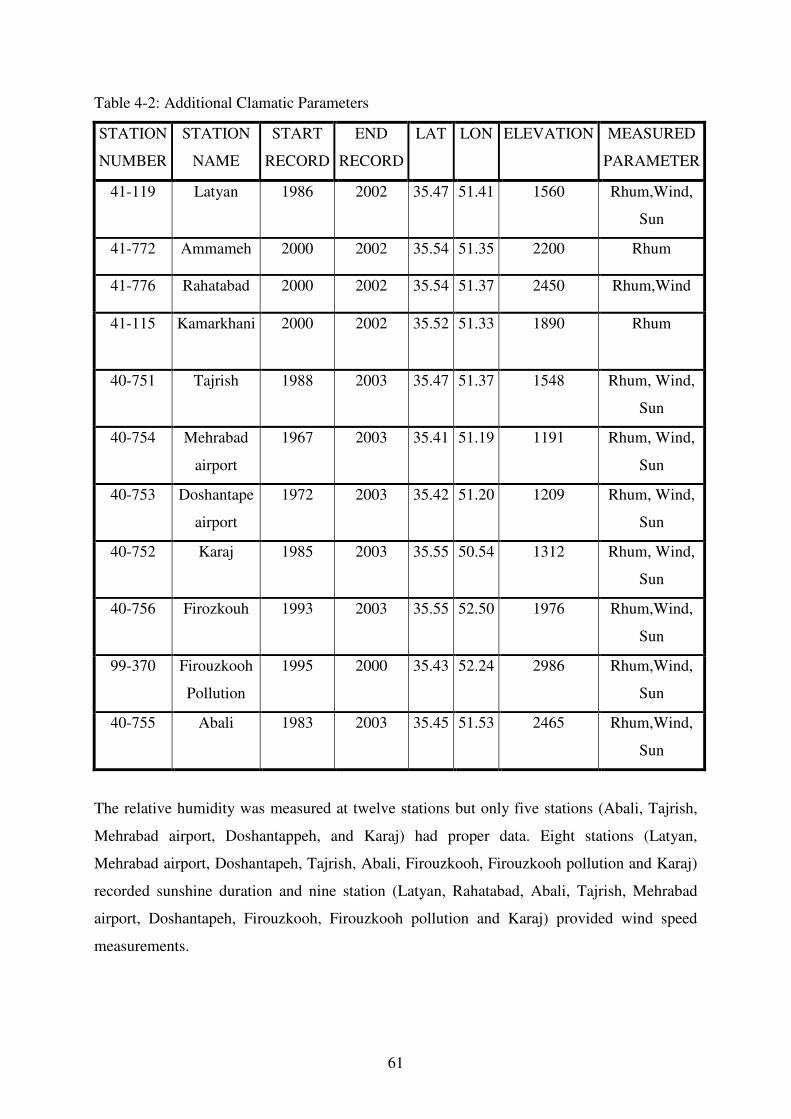
61
Table 4-2: Additional Clamatic Parameters
STATION
NUMBER
STATION
NAME
START
RECORD
END
RECORD
LAT LON ELEVATION MEASURED
PARAMETER
41-119 Latyan 1986 2002 35.47 51.41 1560 Rhum,Wind,
Sun
41-772 Ammameh 2000 2002 35.54 51.35 2200 Rhum
41-776 Rahatabad 2000 2002 35.54 51.37 2450 Rhum,Wind
41-115 Kamarkhani 2000 2002 35.52 51.33 1890 Rhum
40-751 Tajrish 1988 2003 35.47 51.37 1548 Rhum, Wind,
Sun
40-754 Mehrabad
airport
1967 2003 35.41 51.19 1191 Rhum, Wind,
Sun
40-753 Doshantape
airport
1972 2003 35.42 51.20 1209 Rhum, Wind,
Sun
40-752 Karaj 1985 2003 35.55 50.54 1312 Rhum, Wind,
Sun
40-756 Firozkouh 1993 2003 35.55 52.50 1976 Rhum,Wind,
Sun
99-370 Firouzkooh
Pollution
1995 2000 35.43 52.24 2986 Rhum,Wind,
Sun
40-755 Abali 1983 2003 35.45 51.53 2465 Rhum,Wind,
Sun
The relative humidity was measured at twelve stations but only five stations (Abali, Tajrish,
Mehrabad airport, Doshantappeh, and Karaj) had proper data. Eight stations (Latyan,
Mehrabad airport, Doshantapeh, Tajrish, Abali, Firouzkooh, Firouzkooh pollution and Karaj)
recorded sunshine duration and nine station (Latyan, Rahatabad, Abali, Tajrish, Mehrabad
airport, Doshantapeh, Firouzkooh, Firouzkooh pollution and Karaj) provided wind speed
measurements.

62
4.2.1.4 Runoff Data
The discharge data was provided by the Iran Water Resources Management Company
(IWRMCO) and Tehran Regional Water Company (TRWCO). Mentioned data are contains
daily and monthly runoff data for the time period 1971 to 2005 eight runoff gauges Latyan
catchment. The catchment outlet is the hydrometric station 41-119 (Latyan), which went into
operation in October 1945 and has been delivering manually and recorder cable since 1945.
4.2.2 Spatial Datasets (GIS-Data)
Hydrogeological investigation over large areas requires assimilation of information from
many sites each with a unique geographic location. GIS maintains the spatial location of
sampling points, and provides tools to relate the sampling data contained through a relational
database. Therefore, it can be used effectively for the analysis of spatially distributed
hydrogeological data and modelling (SHAHID AND BEHRAWAN, 2008).
The version of J2000g model uses distributed model entities as input. These entities are based
on the concept of the HRUs (FLÜGEL, 1995; FLÜGEL, 1996) using GIS-datasets of land
cover, soil, geology as well as a DEM. The datasets used in this study are summarized in
Table 4-3. The Shuttle Radar Topography Mission (SRTM) dataset (U.S. GEOLOGICAL
SURVEY EROS DATA CENTER AND NASA, 2007) provided information on topography
parameters such as elevation, slope and aspect. Additionally, it was used to delineate the
stream network, catchment borders and sub catchments. Information on soil type was derived
using land capability and resources evaluation map of province Tehran (1991) from the
Ministry of Agriculture of Iran, Soil and Water Research Institute (SWRI).The map as
mentioned, contains difference datasets of province of Tehran mentioned Latyan Catchment
as landtype, soil texture for the soil types, soil classes with (FAO) classification and capability
and limits of lands. The geological information was derived form geological map of Iran
series 1:100000, Tehran(1996), East of Tehran(1997), Damavand(1997), Baladeh(1993),
Marzanabad(2001) sheets from the ministry of Mines and Metals of Iran, Geological Survey
Organization of Iran(GSI), and from SHESHANGOSHT ET AL., (2006). The land cover and
land use parameters (vegetation type and another utility) were obtained using the National
Cartographic Center of Iran (NCC), and from SHESHANGOSHT ET AL., (2006) and
ZEINIVAND AND DE SMEDT (2008).

63
Table 4-3: GIS-dataset for HRU- delineation
Dataset Description Format Resolution Source Model -
Parameter
DEM
Shuttle Radar
Topography
Mission(SRTM)
Raster
90m²
US Geological
Survey(2007)
Elevation
Slope, Aspect
Stream
network
Geology
Geological maps
(Tehran, East Tehran,
Damavand, Baladeh)
Vector
1:100.000
Geological
Survey
Organisation,
Iran(GSI),
(1993, 1997,
2001)
Bedrock
Characteristic,
Maximum
Perculation
Soil
land capability and
resources evaluation
map of province
Tehran
Vector
1:250.000
Soil and Water
Research
Institute(SWRI)
, Iran, 1991
Soiltype,
Soil texture
Land
Cover
Topographic, Maps
Block 15, Tehran
Province, 2004
Vector
1:50.000
National
Cartographic
Center(NCC),
Iran, 2004
Vegetation
Type,
Vegetation
height
For the HRU delineation, all datasets should have the same spatial resolution as well as
projection. Therefore, all datasets were transformed into the UTM-Projection, Zone 39 North
with a spatial resolution of 90 m. Datasets, having a coarser spatial resolution, such as soil
information, land cover, and geology have been resampled in ArcGIS 9.3 (ESRI, 2008) using
the nearest neighborhood method.

64
5. RESULTS AND DISCUSSION

65
In this chapter, the results of the study will be presented. The chapter is divided into three
sections. First, in the data analysis section (Section 5.1.1), the input data will be checked for
missing values as well as for plausibility. Subsequently, a system analysis will be carried out
to investigate the data for indications of an influence on the hydrological response. Second,
the conclusion drawn from this analysis will be used for the model calibration and validation
(Section 5.2). The modelling outputs will also be investigated for their sensitivity to parameter
changes. The conclusions will later be used to assess the snowmelt modelling results. Third,
to compare the simulated SWE single HRU stations with the SWE time series, the area under
investigation had to be determined (Section 5.3.1). After doing so, the model entities lying in
this area of interest are averaged using the area weight, and then compared to the SWE time
series (Section 5.3.2). In this step, similarities and variations in long term (trend) and short
term (seasonal) SWE will be highlighted. This analysis will give an insight on the evolution
of the snowmelt and SWE modelled time series and therefore information on future behavior
can be drawn. Based on these results, the capability of the model J2000g for snowmelt
modelling will be analyzed.
5.1 System Analysis and Delineation of Hydrological Response Units
5.1.1 Data Analysis and System Analysis
5.1.1.1 Precipitation Data Analysis
As documented in Section 4.2.1.1, the rainfall data needed in this study were collected by
WSIMO and IWRMCO. The 24 rainfall stations (Figure 4-9) in and surrounding the
catchment area were extracted from this database and used in this study. As discussed in
Section 4.2.1.1, the data filled using a combination of algorithms such as inverse distance
weighting, linear regression techniques.
For each station the long term monthly and yearly statistical parameters mean, minimum,
maximum and standard deviation were calculated for the time frame from 1970 to 2004. The
long term mean annual precipitation amounts to between 420 and 563 mm with a standard
deviation ranging from 96 mm to 143 mm. The regression analysis reveals a very strong
positive relationship between the standard deviation and the mean values (R² = 0.85). In other
words, the year-to-year variability increases with an increasing mean annual rainfall.

66
5.1.1.2 Discharge Data Analysis
The double mass approach, explained in the Section 3.1.1.1, has been applied to analyze the
runoff observation between stations along the Latyan catchment stream. Figure 5-1 shows the
double mass–analysis between the runoff stations Latyan and Roodak as well as Naran and
Najarkola(Galandoak), whose locations are shown Figure 4-1.
The left hand side of Figure 5-1 shows the double mass curve between the catchment outlet
(Latyan) and the Roodak station, located approximately 3km upstream from the Latyan
station. On the right hand side of the figure, the double mass curve between the Naran and the
Najarkola stations is illustrated. The Naran measuring station records the discharge of the
Naran River, a tributary to the Latyan Dam Lake. The Najarkola runoff station lays about 1
km before the Naran River joins the Latyan Dam Lake. The two runoff stations are
approximately 1.5 km apart from each other, shown in Figure 4-1.
0
500
1000
1500
2000
2500
3000
3500
4000
0 500 1000 1500 2000 2500 3000 3500
acc. Q. Latyan(m³/s)
acc. Q
. R
oo
dak(m
³/s)
0
500
1000
1500
2000
2500
3000
3500
0 50 100 150 200 250
acc. Q. Najarkola(m³/s)
acc. Q
. N
ara
n(m
³/s)
Figure5-1: Dubble Curve Mass Analysis in the Latyan Catchment
The double mass curve on the left side of Figure 5-1, shows that runoff relationship between
the two station had been changed, and “more” runoff has been recorded at the outlet station
(Latyan) than at the upstream station (Roodak) within the 1970 to 2004 time frame. The
comparison of this curve with the mean annual precipitation-data indicates that these
characteristics could be explained by anthropogenic influences and natural factors like long
time droughton the river discharge. The first section marks the time period until the end of
1982, characterized by an above average mean annual precipitation (MAP) (Figure 5-2). The
years from 1980 to 1989, with the exception of one year 1982 are characterized by low
precipitation, whereas the years from 1972-78 and 1996-2001 show above average MAP.The
changes in slope can be explained by water uptake along the river before the Roodak station
or technical measuring problems, especially during the years with low precipitation (1970 to
1992).

67
This argument of anthropogenic impacts on the stream flow volume is supported by the
analysis of the second double mass curve on the right hand with same condition of graph
This double mass analysis indicates intensive anthropogenic regulation of the discharge and
natural condition of drought. The discharge in the river stream is especially ruled by the major
dams, Latyan dam, located in the outlet of the catchment. To reduce the anthropogenic
influence in the rainfall-runoff modeling, the catchment area of the dams was not taken into
model calibration.
5.1.1.3 Temporal Relationship between Precipitation and Discharge in the
Latyan Catchment
The hydrological modelling of the catchment of Latyan requires an understanding of the
natural as well as anthropogenic influences on the runoff generation as shown in the
preceding analysis. The rainfall-runoff interaction analysis was carried out for a longer time
period (1970-2004) than in the actual study (1990-2001). This was done to gain more
information on the system. The investigation focuses on the annual, seasonal and monthly
temporal scale.
Figure 5-2 compares the long term mean annual precipitation (blue bars) to the annual runoff
sum (blue line), as well as the variation from the 34 years average for rainfall (blue filled
bars) and runoff (blue unfilled bars).
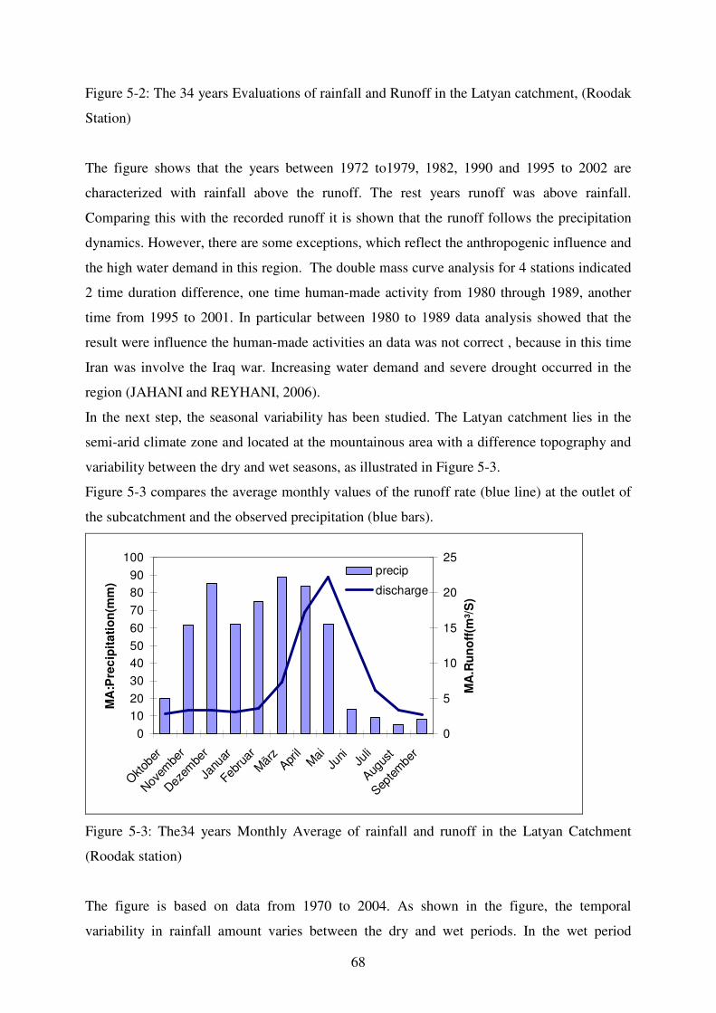
68
Figure 5-2: The 34 years Evaluations of rainfall and Runoff in the Latyan catchment, (Roodak
Station)
The figure shows that the years between 1972 to1979, 1982, 1990 and 1995 to 2002 are
characterized with rainfall above the runoff. The rest years runoff was above rainfall.
Comparing this with the recorded runoff it is shown that the runoff follows the precipitation
dynamics. However, there are some exceptions, which reflect the anthropogenic influence and
the high water demand in this region. The double mass curve analysis for 4 stations indicated
2 time duration difference, one time human-made activity from 1980 through 1989, another
time from 1995 to 2001. In particular between 1980 to 1989 data analysis showed that the
result were influence the human-made activities an data was not correct , because in this time
Iran was involve the Iraq war. Increasing water demand and severe drought occurred in the
region (JAHANI and REYHANI, 2006).
In the next step, the seasonal variability has been studied. The Latyan catchment lies in the
semi-arid climate zone and located at the mountainous area with a difference topography and
variability between the dry and wet seasons, as illustrated in Figure 5-3.
Figure 5-3 compares the average monthly values of the runoff rate (blue line) at the outlet of
the subcatchment and the observed precipitation (blue bars).
0
10
20
30
40
50
60
70
80
90
100
Okt
ober
Nov
embe
r
Dez
embe
r
Janu
ar
Febru
ar
Mär
zApr
ilM
ai
Juni Ju
li
Augus
t
Septe
mbe
r
MA
:Pre
cip
ita
tio
n(m
m)
0
5
10
15
20
25
MA
.Ru
no
ff(m
³/S
)
precip
discharge
Figure 5-3: The34 years Monthly Average of rainfall and runoff in the Latyan Catchment
(Roodak station)
The figure is based on data from 1970 to 2004. As shown in the figure, the temporal
variability in rainfall amount varies between the dry and wet periods. In the wet period

69
(November to May) about 518 mm, corresponding to 90 % of the annual rainfall, are
recorded. In the dry season (June to September) the measured monthly rainfall amounts to less
than 56 mm, whereas during June to August only 13 to 5 mm precipitation are documented.
The high temporal variability is also reflected in the runoff, as shown in the differences
between the low flow and high flow seasons (Figure 5-3). During the dry season, the average
monthly flow rate fall under2.6 m³/s. It indicated that in dry season catchment rivers are
related to snow melt runoff for the river. The wet season, however, is characterized by low
discharge values but with a runoff peak in the May and not corresponds to the precipitation
peak. It can be concluded that more than precipitation of catchment fall as snow and Runoff
River is related to snowmelt.
5.1.2 Spatial Dataset
Table 4-3 shows the datasets used to delineate the HRUs used in the model. In order to
achieve a common spatial resolution the raster datasets, land cover and the DEM, were
resampled to 90 m. The vector datasets, the soil data and the geology dataset, were converted
into raster files with a resolution of 90 m by applying the nearest neighbour method. All GIS-
data files were than transformed into the UTM Projection, Zone 39 North.
The DEM delineated from the SRTM-data (U.S. GEOLOGICAL SURVEY EROS DATA
CENTER AND NASA, 2007) was used to derive topographical parameters such as aspect and
slope. Therefore, the dataset had to first be prepared and sinks had to be filled (WOLF, 2009)
with the “fill” routine implemented in ArcInfo within ArcGIS Destop 9.3 (ESRI, 2008).
Afterwards, flow direction and flow accumulation were delineated in ArcInfo within ArcGIS
Desktop 9.3 (ESRI, 2008). An accumulation threshold of 250 cells was used for the
delineation of the stream network. The resulting stream network was compared visually to the
available topographic maps and corrected if necessary. Afterwards, the sub catchments were
delineated using the Spatial Analyst Tools within ArcGIS Desktop 9.3 (ESRI, 2008). The
location of available hydrometric stations was corrected so that the runoff stations were
located on the delineated stream network. As a result, 4 sub catchments with areas from 31 to
430 km² were delineated.
The hydro-meteorological time series (Table 4-1, Table 4-2) are representing measurements at
point scale. To obtain spatial information for these hydro-meteorological parameters, the
measurements had to spatially generalized using the IDW- method implemented in J2000g
(KRAUSE, 2001; JAMSWIKI, 2010) described in Section 3.2.1.

70
5.1.3 Delineation of Hydrological Response Units
The delineation of the HRUs consists of several steps, as shown in Figure 5-4 In the first step
the individual GIS-datasets will be reclassified according to their hydrological significance.
Then the prepared datasets will be overlaid on one another and, if necessary, reclassified
again. Afterwards, small polygons under a certain threshold will be aggregated into
neighboring polygons
Finally, the resulting HRUs will act as model entities in the hydrological model. The
following sections give a more detailed description of these steps.
Figure 5-4: Flow-chart of the Delineation of HRUs for the J2000g model (Source:
SCHEFFLER, 2008)
5.1.3.1 Data Preparation and Reclassification
The first step of the HRU-delineation involves data preparation and reclassification of the
GIS-datasets. This is necessary to meet the requirements for the hydrological model
(KRAUSE, 2001:P. 140). The single values of the topography, slope, aspect, geology, and
soil and land cover datasets are reclassified according to their hydrological importance to
reduce the number of HRUs.
The slope values were grouped into the following classes: low slope areas (0-5°), medium
slope areas (5- 15°) and high slope areas (>15°) according to the work of BONGARTZ
(2001). For the aspect, classes modified from BONGARTZ (2001) HELMSCHROT (2006)
and SCHEFFLER (2008) have been used, as shown in Table 5-1

71
Table 5-1: Reclassify the aspect
Class Descrption Aspect in°
North 337.5 – 360; 0 – 22.5
Northeast 22.5 – 67.5
1
Northwest 292.5 – 337.5
Southeast 112.5 – 157.5
South 157.5 – 202.5
2
Southwest 202.5 – 247.5
West 247.5 – 292.5 3
East 67.5 – 112.5
Due to no specific soil data available for the Latyan catchment, a soil map and other
information on soil type was derived using land capability and resources evaluation map of
province Tehran, Iran from Soil and Water Research Institute (SWRI, 1991). First the soil
map of (SWRI) georeferenced using georeferencing tools of ArcMap ArcGIS 9.3(ESRI,
2008), then the boundary of catchment and soil classes were digitized using edit tools of
ArcMap ArcGIS 9.3(ESRI, 2008).After analyzing the available soil dataset (SWRI, 1991), the
following classes for the catchment were delineated .
Table_5-2 Classification of the Soil Types (Source: SWRI, (1991))
Soil Group FAO Soil Type Description
1(11) Lithic and Eutric Leptosols, Calcaric
Regosols
Very shallow to fairly shallow, with coarse sand, medium to coarse texture
2(12) Lithic Leptosols, Calcaric Regosols
Fairly shallow in peaks, semi shallow with fine sand in slopes
3(21) Lithic Leptosols, Eutric Leptosols,
Very shallow soils, without soil cover
4(32) Calcaric Regosols Fairly shallow to deep, with fine sandy and medium to coarse texture, with many lime
According to SCHEFFLER (2008) all soil groupes mentioned above summarizes soils with
clay content between 10 to 25 %, including the Leptosol and Regosol soil types.
Distinction between the major land cover classes was made based on vegetation properties,
like leaf area index, vegetation height, rooting depth, and stomata resistance.
The land cover information was grouped into land cover classes, shown in Table 5-3.

72
Table5-3: Classification of the Land Cover Classes (Source: NCC, (2005))
Land Cover Class
Land Cover Classes Description
Agriculture 3, 4, 15 Dry farming, Irrigated Farming, Paddy and other agricultural land
Decidous broad trees
13,5,9,10,14 Woodland, A forestation, Orchard, Indigenous Forest, Forest plantation of Plane tree, single trees
and others Decidous
shrubs 22,2,1 Shrub, Thicket and Bush, Degraded Land (areas
with low vegetation)
Grassland 12,17 Grass, Pasture, Urban Area Grassland
Settlement 8, 25,27 Rural Area(residential), Urban Area(commercial, residential, build up)
Water 6 Water, Lake dam
The available geology information was grouped into only two classes, shown in Table 5-4.
Table 5-4: Stage of Geology Classification
Class Description GSI Code
Sedimentary Rocks Black limestone, clayey marl intercalation, Light grey massive dolomitic limestone, Black oolitic and intraclastic limestone,
Sandstone , shale, limestone, marl, phosphatic layers
Cbj, Ccj, Cdj, Daj
Sedimentary Rocks Black massive dolomite, green-black shale intercalations, Red
arkosic sandstone, Micaceous red siltstone, redsandstone, Trilobite bearing limestone, marl, dolomite and shale,
Quartzitic sandstone
Єdbt, Єl, Єz, Єm, Єq
Sedimentary rocks Calcareous and siliceous dark colored shale, Cream-bedded to
massive limestone,dolomite,chertly, Thin-bedded marly limestone,marl,Amonite bearing, Thin-bedded to massive
limestone
Eshk, Jl2, Jd, Jl
1
Sedimentary rocks Gray,yellow, green,lime.,argilaceus lime.,marl, Light
gray,medium-thick bed limestone.,argilaceus limestone, Orbitolina limestone(Aptian- Albian), Miliolids limestone,
gypsum, conglomerate, siltstone, sandy marl
K1_M, K1t, Kt M

73
Sedimentary rocks Thick-bed to massive polygenetic conglomerate, sandstone,
locally limestone beds, Alveolina-nummulitic limestone, conglomerate, gypsum, Sandstone, shale, limestone
intercalations, Mudstone intercalations, fusolina limestone, dolomitic limestone
PEcf, PEI, PEz, Pd,
PIQcs Pr
Sedimentary rocks Young-old screeslope, talus, deposit, aluvial fan, Landslide, rockfall, rock stream, Shale, sandstone, siltstone, claystone, coal bearing, Massive dolomite, Thick-bedded to massive
limestone
Q, Q1, QI, TR3Js,
TRde, TRIe
Igneous Rocks Basaltic-andesitic lava flows, White-green tuff breccia, ash tuff,
Green thick-bedded tuff, minor lava, pyroclastics, Volcanic rocks locally basic, agglomerate, tuff,
Dvj, Eb, Etk, Evk
2
Igneous Rocks Volcanics includ basalt and spilite, Volcanics, pyroclasics, tuffs, Basic and intermediate sills, Mostly syenite and some
leucosyenite porphyry
Kv, Pe, PEvf, Tb, Ts

74
5.1.3.2 Overlay Analysis and Reclassification
The overlay of the GIS-datasets was carried out in successive stages as shown in Figure 5-4.
The first overlay (aspect and slope) build Topography-Set (TS) entities.
In second overlay the Landcover-Soil-Set (LSS) were created by overlaying soil and land
cover. Afterwards, the resulting LSS was overlaid with the TS. In this step, first the rock
classes from deciduous shrubs separately combined as constant classes. Additionally, in forest
classes with a slope below 5°, the east / west aspects have been transformed to a north aspect.
SCHULZE, MAHARAJ ET AL. (1997:P.29-30 analyzed the solar radiation on different
slopes and aspects. They founded that with a slope below 5° the radiation amount for North,
NE/NW, as well as E/W facing aspects was comparable, whereas SE/SW and South facing
aspects with the same slope showed a much higher radiation input. This has only been applied
to areas with dense vegetation, such as forest (SCHEFFLER, 2008:P.88). In the last step of
the successive overlay processes the resulting Topography-Soil-Vegetation Complexes were
overlaid with the geology groups. As a result of the generalization process 18113 HRUs were
defined for the Latyan catchment.
5.1.3.3 Generalization and Delineation
After finishing the knowledge based aggregation, the resulting entities were overlaid with the
sub catchments. The smallest polygons with an area below 5 Raster Cells (<0.05 km²), were
then eliminated using the Dissolve Adjacent Polygons in Data Management Tools in ArcMap
9.3(ESRI, 2008). The 18113 HRUs were generalized to 5369 HRU-Polygons and used as
modelling units for the J2000g model. The physical characteristics were assigned using the
majority function for land cover, soil and geology. For elevation, slope and aspect mean
values were computed using the Arc Info Arc GIS 9.3 (ESRI, 2008).
5.2 Snowmelt–Runoff Modelling using J2000g model
5.2.1 Model Parameterization

75
The model requires separate parameter files for land cover, soil and ground water. Each land
cover class consists of 5 land use parameters, each soil class of 2 soil parameters and each
hydrogeologic class of 1 groundwater recharge parameters. The parameter values were taken
from literature values and are explained in more detail in the following sections. (KRAUSE
AND HANISCH, 2009)
5.2.1.1 Landuse-Land Cover Information
Because, the advantage of the Penman-Monteith method is the higher physical basis, in this
study, the J2000g model calculates the evapotranspiration and potential evaporation rate
based on the Penman-Monteith approach (JAMSWIKI, 2010). This approach estimates the
evapotranspiration in the canopy layer using several vegetation parameters such as leaf area
index (LAI), stomata resistance, rooting depth, and vegetation height. This information was
retrieved from literature values, shown in Table 5-4 B in Appendix B for land cover classes.
5.2.1.2 Information on Soil Data
The soil information was extracted from description of land capability and resources
evaluation map of Tehran province, Soil and Water Research Institute (SWRI).That
description contains difference datasets of province of Tehran mentioned Latyan Catchment
as landtype, soil texture for the soil types, soil classes with (FAO) classification and capability
and limits of lands. The database did not contain any field probe and more detail of soil within
the study area. To achieve representative soil texture characteristics for the soil types found in
the study area, the available soil texture information was averaged according to the soil type
properties of WRB, and FAO, ISRIC (2006) and later the values for each soil type were
averaged according to the soil groups.
The soil water module of the J2000g model has two parameters namely depth of the soil in cm
and entire usable field capacity of the soil in mm. For better accuracy of extracting of
mentioned soil parameters the land cover and vegetation cover of the Latyan catchment was
used. Therefore, in areas with high vegetation cover, the soil parameters were adapted.
Namely in the areas with vegetation covers, both depth and FC sum parameters is increased.
The soil parameter values shown in the table 5-5

76
Table 5-5: Parameters of the Soil Classes for the Soil Water Module
Soil Class Depth [cm]
FC sum [mm]
111 120 73.17
11 60 10.66
112 130 211.5
12 60 21.3
121 60 21.3
21 60 10.66
132 130 211.5
32 130 211.5
5.2.1.3 Information on Geology Data
In the geology data, for each hydrogeologic unit the maximum possible ground water
recharge rates per time unit are set up. It only contains the following two attributes: GID - a
clear numeric ID with which the connection to the model unit table is generated. mxPerc - the
maximum possible percolation rate (ground water recharge rate) per time interval in mm per
time unit(JAMSWIKI, 2010).
Due to poor information about maximum possible percolation of difference geological classes
in the catchment and due to simplify component of ground water recharge in the j2000g
model for both hydrogeological classes an constant parameter value about 28 was input to
hydrogeology parameter of model( Table 5-6) .
Table 5-6: Parameters of the Geology classes for the Ground Water Module
Geology Class Max Percolation [mm]
1 28
2 28
77
5.2.2 Model application, calibration and evaluation
5.2.2.1 Model application
To provide spatially consistent input information for J2000g, the Latyan catchment was
partitioned into 5369 modelling units (HRUs) resulting from a GIS overlay of slope, aspect,
land-use, soil type and hydrogeology. Slope and aspect were classified into five and three
classes in advance. After the GIS overlay, the centroid coordinates, area, mean slope, most
frequent aspect, soil type, land-use and hydrogeological type were extracted for each unit and
transformed into a J2000g compliant data table. The soil type and the land-use information are
correlated to specific tables during model initialisation to derive physical values for field
capacity and vegetation-specific parameters such as the stomatal resistances for good water
availability and the leaf-area-index. Monthly values of observed climatological input data
(temperature, precipitation, relative humidity, sunshine hours, and wind speed) from the
meteorological stations shown in figure 4-9 were transferred to each modelling unit using data
from the five closest stations. Values of the six J2000g parameters (FCA, Tbase, TMF, LVD,
ETR and GWK) had to be estimated through a model calibration procedure. The calibration
was done for 3 subbasin within the Latyan catchment boundaries with sufficient streamflow
observations. The selection of suitable subbasins was complicated by the fact that J2000g
does not explicitly recognize man-made influences on the hydrological processes and does not
account for water losses in karst regions both relevant factors for the runoff amount in some
parts of the Latyan catchment. As a result, only subcatchments with minimal man-made
influence and primarily impermeable bedrock conditions were selected for calibration.
Therefore, three subbasins were selected for calibration: Roodak, Najarkola, and Naran. The
extent area of these subbasins ranges between 31 to 430 km2 (see figure 4-2). For each
subcatchment, values for the six model parameters were calibrated automatically using the
Monte-Carlo-Analysis runs and Shuffled Complex Evolution – University of Arizona (SCE-
UA) method (Duan et al., 1994). Both methods adapt a selected number of model parameters
in order to optimise a single objective function or efficiency criteria. The calibration was done
with observed monthly climate values for the time period from October 1990 through
September 2001 using the Nash-Sutcliffe efficiency (NSE) measure as main objective
function. The calibrated parameter values are shown together with the resulting NSE values in

78
Table5-7. Table5-7, column CV indicates that the degree of variability among the three
subcatchments varies for each parameter. The values for TMF and Tbase vary the least for all
subbasins, probably because they are the most “physically based” and are largely independent
from other factors in the catchment. The low values of Tbase is caused by the monthly
modelling time steps because, Tbase represents the mean monthly temperature which has to
be considerably below 0 C° to store precipitation as snow for a longer period than one time
step of one month(KRAUSE AND HANISCH, 2009).
The value for parameter ETR also indicates relatively low variability among the
subcatchments. But the NSE, however, was very sensitive to Tbase, TMF and LVD
parameters. The remaining parameters GWK, FCA, and LVD exhibit considerably more
variability among the catchments compared to the other three parameters. However, the NSE
was not very sensitive to changes in GWK (or FCA and ETR) which accounts for the wide
range in values. The NSE values for three of subcatchments were computed between 0.78 and
0.82 which demonstrates that J2000g simulates the observed streamflow reasonably well in
the calibration period.
For the all Latyan catchment application of J2000g it was assumed that one “global”
parameter set could be derived from the calibrated parameter values from the three calibration
subcatchments that would result in “reasonable” estimates for the entire study area. This
global set was obtained by an area-weighted mean of the parameters of the model parameters
carried out for the three test catchments. To test the global parameter set it was first used in
each of the three calibration subbasins for the same time period used for the calibration. The
resulting NSE value (NSE (gps)) for each catchment is also shown in Table 5-7 Although
there was least reduction in model performance for each subcatchment, the range of NSE
(gps) values (0.68 and 0.79) is relative close to those obtained with the optimal parameter
values for two of the three subcatchments.
5.2.2.2 Validation
The application of the global parameter set in the three calibration catchments resulted in the
conclusion that the J2000g model is fairly robust with an acceptable degree of certainty based
upon model calibration. To test if the model is also producing reliable results for other time
periods and other catchments, the global parameter set derived in the calibration catchments
was used in the Roodak subbasin for the longer period from October 1972 through September
2003. The simulated streamflow values were aggregated as long-term mean monthly average

79
values and compared to observed streamflow records of Roodak gauge. The result is shown in
figure 5-5
The figure shows the observed (blue) and simulated (red) long-term monthly runoff for
Roodak subbasin which is very similar to whole catchment.The plot indicates that J2000g is
able to reproduce the historical 31year long-term monthly runoff values quite well for all
Latyan catchment. It should be emphasised that these results were obtained with the global
parameter set resulting from the calibration in three subcatchments.
0
5
10
15
20
25
30
35
40
45
50
Oct 72
Mar
74
Aug 7
5
Jan 7
7
Jun 7
8
Nov 7
9
Apr
81
Sep 8
2
Feb 8
4
Jul 8
5
Dec 8
6
May 8
8
Oct 89
Mar
91
Aug 9
2
Jan 9
4
Jun 9
5
Nov 9
6
Apr
98
Sep 9
9
Feb 0
1
Jul 0
2
Mean
mo
nth
ly Q
m³/
s
Simulated
Observed
Figure 5-5: Result of the validation of J2000g for Roodak subbasin in the Latyan catchment
The plot shows the long-term monthly simulated (red line) and observed (blue line)
streamflow of the period from 10/1972 to 09/2003.

80
Table 5-7 SubCatchment areas, J2000g parameter values from Monte-Carlo-Analysis and
SCE optimisation along with best Nash-Sutcliffe efficiency (NSE) obtained and the
efficiencies achieved with the global parameter set (NSE(gps)) for the calibration catchments.
The last column shows the coefficient of variation (CV) of the calibrated parameter values.
The values of this table were obtained with the calibration period from 10/1990 to 09/2001.
Table 5-7: SubCatchment areas, J2000g parameter values from Monte-Carlo-Analysis and
SCE optimisation
CATCHMENT ROODAK NAJARKOLA NARAN gps CV%
AREA(km²) 430.93 60.95 31.05 --- ---
LVD 1.22 3.58 1.73 1.53 47
GWK 7.73 5.98 2.23 7.2 43
Tbase - 3.07 - 2.2 -2.56 - 2.94 14
TMF 19.77 18.97 17.89 19.57 4
FCA 12.26 4.78 17.57 11.70 45
ETR 0.41 0.61 0.74 0.45 23
--- --- --- --- --- --- NSE 0.82 0.78 0.79 --- ---
Log.NSE 0.80 0.65 0.76 --- --- PBIAS - 5.6 - 2.2 7.1 --- ---
r² 0.83 0.78 0.81 --- ---
NSE(gps) 0.79 0.68 0.77 --- ---
Additional calibration of the internal model processes was performed with measured snow
water equivalent (SWE) of nine climate stations which lies inside the Latyan catchment. The
measured SWE data were compared with the SWE simulated on single HRUs which had
difference elevation and are located inside and around the three subcatchments. Figure shows
the simulated SWE as a red line and the measured values as blue line for the ten years of the
calibration period. The figure shows that the model is able to reproduce the development of
the snow pack of the catchment very well. The rising limb of the snow accumulation period is
captured nearly perfect despite the year 1996 as it is the maximum snow amount (despite
1996 and 1997). Obviously the snow module is defined as simplify (temperature-index)
model, therefore simulated results can be accepted as good prediction. As the snow melt
dynamics are responsible to a high amount for the runoff dynamics in the Latyan catchment it
can be concluded that the snow modelling has a large influence on the model performance.

81
This is highlighted by the fact, that the four years which showed the lowest efficiencies (1997,
1999, 2000, 2001) of the validation period are also those where severe problems in the snow
modelling are obvious. It is comparable that, during this time, the water table is suffering
from a continuous decline as a result of the critical situation in available water resources and
low flow condition and drought in Tehran as well as most parts of the Iran (JAHANI AND
REYHANI, 2006).
The brief description of the case study showed that the model is able to reproduce the
hydrological dynamics of a mountainous catchment quite well. This is of importance in
relation to the mesoscale applications in the Latyan catchment; because it shows the
transferability of the current process simplify modules to different scales. Nevertheless the
relevant hydrological dynamics can be simulated by the model with a certain degree of quality
as the results show.
Table 5-8, shows the estimated water balance components for the 11 year period (October
1990 to September 2001). According to this table there is no substantial difference between
the model results for 3 subcatchment. Notice that for all the Latyan catchment, the snowfall
constitutes almost half of the total precipitation, and consequently snowmelt has a large
impact on the river discharge. The main period of precipitation occurs during late autumn till
late winter, while river flow rises gradually in early spring to reach peak values in May. From
the foregoing it can be concluded that the runoff occurs mainly from March till June
depending upon the air temperature, indicating that most of this runoff is generated by
snowmelt.
For discussion two interesting periods is selected with large and small snow accumulation and
melt. The first period is from October 1992 to September 1993 for large snow and from
October 2000 to September 2001 for small snow. All relevant information for these periods is
given in Figure 5-6.

82
0
50
100
150
200
250
300
350
400
450
500
Oc
t 9
2
No
v 9
2
De
c 9
2
Ja
n 9
3
Fe
b 9
3
Ma
r 9
3
Ap
r 9
3
Ma
y 9
3
Ju
n 9
3
Ju
l 9
3
Au
g 9
3
Se
p 9
3
mm
-10
-5
0
5
10
15
20
25
P rec ipitation
S WE
S nowmelt
Tmean °C
0 °C
[°C ]
Figure 5-6: Monthly precipitation, mean air temperature, snow water equivalent and
snowmelt, Roodak subbasin, J2000g model simulation, 1992-1993.
The degree day method assumes that all precipitation falls as snow when the mean
temperature of the subcatchment is lower than Tbase and as rain when the temperature is
higher than Tbase. The mean temperature in the catchment drops below zero from December
till end March, and accordingly only snowfall occurs and the snowpack gradually builds up to
reach about 438 mm of water equivalent at the first March, while there is almost no snowmelt.
From end of March, the temperature becomes positive and about 119 mm of snow melts.
From mid April till first May, increase temperature continues and snowmelt increase to 152
mm. Finally, at the end of July all snow has completely melted. It to be noted that, the
snowmelt finish earlier July in dry years with low precipitation and high temperature.
0
20
40
60
80
100
120
140
160
Oc
t 0
0
No
v 0
0
De
c 0
0
Ja
n 0
1
Fe
b 0
1
Ma
r 0
1
Ap
r 0
1
Ma
y 0
1
Ju
n 0
1
Ju
l 0
1
Au
g 0
1
Se
p 0
1
[mm
]
-10
-5
0
5
10
15
20
25
P rec ipitation
S WE
S nowmelt
Tmean °C
0 °C
[°C ]

83
Figure 5-7: Monthly precipitation, mean air temperature, snow water equivalent and
snowmelt, Roodak subbasin, J2000g model simulation, 2000-2001.
The figure 5-7 clearly showed the fluctuations of snowmelt in the dry year of 2000-2001. In
this time all the study area and Tehran covered by severe drought (JAHANI and REYHANI,
2006). In addition revealed that the condition of snowmelt and SWE is not constant in the
Latyan catchment and snowmelt in end of May is finished
Figure 5-8 shows a graphical comparison between observed and computed Runoff at Roodak
subcatchment. In the figure the blue line represents the observed runoff and the red line
represents the simulated runoff. The Parameter values used to simulate the runoff are shown
in table 5-7. From the graphs of simulated and observed runoff curves, it can be seen that the
model can faithfully simulated the both high and low flow. Also the model is found to
simulate the recession limb very efficiently. Howevere, in all the cases NSE was moderately
high (0.82) which means that the model traced very well agree with the observations.
0
5
10
15
20
25
30
35
40
45
Oct 9
0
Ma
y 9
1
De
c 9
1
Ju
l 9
2
Fe
b 9
3
Se
p 9
3
Ap
r 9
4
No
v 9
4
Ju
n 9
5
Ja
n 9
6
Au
g 9
6
Ma
r 9
7
Oct 9
7
Ma
y 9
8
De
c 9
8
Ju
l 9
9
Fe
b 0
0
Se
p 0
0
Ap
r 0
1
Me
an
mo
nth
ly Q
m³/
s
SimulatedObserved
Figure5-8: Graphical comparison between simulated and observed Runoff at Roodak
subcatchment in the Latyan catchment, from 10.1990 through 09.2001
5.2.2.3 Verification of the Modeling Results

84
The simulated snowmelt values range between 199 mm and 730 mm and, in conjunction with
precipitation amounts between 557 mm to 1376 mm, which results in a snowmelt/rainfall
ratio of 36 to 53 %. In other words, between 36 % and 53 % of the precipitation is falled as
snow and melted. Hence, the snowmelt values are indicated that snow is important
hydroclimatic factor in the catchment. Similar ranges for the percentage of snow were
achieved by SHAFIEE (1999) and water and energy research institute (WEI) (2004).
SHAFIEE calculated snow ratio of the Northern part of Tehran in his research about snow
hydrology. He calculated values showing that between 35 to 57 % of the winter and annual
precipitation of this region is falled as snow.
Figure 5-9: Mean Annual Runoff. Modelled using the J2000g Model
In addition computed evapotranspiration values are between 267 mm and 463 mm, which
results in an evapotranspiration/rainfall ratio indicated that, between 34 % and 48 % of the
precipitation water is evapotranspired. The estimated actual evapotranspiration was compared
to estimated actual evapotranspiration values found in FARAMARZI ET AL., (2008). The

85
values of 267 mm to 463 mm for the entire modeled period are within the estimated range of
211 and 780 mm for the Tehran Province.
Figure 5-10: Mean Annual Actual Evapotranspiration. Modelled using the J2000g Model
Also comparison of coefficient variation(CV) between predicted and observed runoff
illustrated that the variation between both values is very low and is about 1% as well as
between snowmelt and precipitation were not high and is as follow about 3 and 11%.
Table xxx illustrates the computed water budget components simulated by the J2000g model
time period from 1990 to 2001.

86
Table5-8: Water Balance Components for the Entire Modelled Period (1990-2001)
YEAR PRECIP
(MM)
POT ET
(MM)
ACT ET
(MM)
SNOWMELT
(MM)
QSIM
(MM)
QOBS
(MM)
1990 - 91 719 753 356 288 329 501
1991 - 92 1376 665 425 730 802 883
1992 - 93 1000 737 401 560 661 754
1993 - 94 967 748 347 342 655 569
1994 - 95 1125 744 415 356 711 829
1995 - 96 984 707 370 470 593 659
1996 - 97 557 765 315 241 311 339
1997 - 98 988 747 463 462 485 565
1998 - 99 604 806 367 244 287 341
1999 - 00 601 782 267 311 332 368
2000 - 01 657 681 415 199 260 234
MEAN 871 739 376 382 493 549
MAX 1376 806 463 730 802 883
MIN 557 665 267 199 260 234
STDEVP 249 40 53 152 189 206
CV % 29 5 14 40 38 37
Spatial distributions of modelled snow water equivalents at the beginning of the winter and at
the time of maximum snow accumulation are shown in Figure 5-11
Figures 5-9, 5-10, and 5-11 indicated that topography slopes as well as aspects played
important role in the rainfall type fall, spatial distribution of snow cover, runoff generation
and adjustment of evapotranspiration in the catchment. Additionally the output result also
revealed the capability of the J2000g in the mountainous area for generation of runoff.Namely
at the time of maximum accumulation; high elevation area and gradients seem to have
dominant effect on spatial distribution of snow. Hence with increasing elevation in the
catchment, the values of snow cover and SWE will increase and maximum of snowpack
distribution and SWE is seen in the high altitude areas. These results comply with the
knowledge of snowmelt spatial distribution in mountains. Thus, the modelled results seem to
be reasonable.

87
Figure 5-11: Mean Annual (1990-2001) Snow Water Equivalent (SWE) Modelled using the
J2000g Model
In addition the various visual modelled results of the model J2000g illustrated a good relation
ship between temperature, topography and, SWE and snowmelt, namely in the Latyan
catchment in low elevation areas in the southern side of catchment like valleys and around
lake dam average temperature is higher than northern side catchment and high altitude.
Therefore the time of snow melt in valleys and lowlands of catchment begins erlier than
northern of catchment. Additionally in the mentioned areas values of SWE is lower than
northern of catchment. In other words, in the end of snowmelt in the southern side of Latyan,
in same time in summer (July to August) the snowmelt exist and continue in the high
elevations like Shemshak and Garmabdar areas. Figure 5-13 show the continuing of snowmelt
on 19th august 2008 near Shemshak.

88
Figure 5-12: Mean Annual Temperature (1990-2001) modelled using J2000g model in the
Latyan Catchment

89
Figure 5-13: snowmelt in the high elevation areas of the Alborz Mountains (source:
http://www.flickr.com/photos/ 2780623124_f0ff04d206_19_aug_2008.

90
6. CONCLUSIONS AND FUTURE RESEARCH

91
6.1 Conclusions and Future Research
A spatially distributed process-oriented hydrological model J2000g was developed and test in
the Latyan catchment, Iran, based on simple temperature-index snow module. The model
performance was tested by simulating snow accumulation and melt in the three sub
catchments.
The model performance was first tested by simulating runoff as well as snowmelt and snow
water equivalent (SWE) in the three subcatchments of the Latyan (Roodak, Najarkola and
Naran) with various extents between 30 through 430 km², in the mountainous area in north-
eastern part of the Tehran, Iran. The model was applied and calibrated with 11 years (1990-
2001) of monthly observed precipitation, air temperature, sunshine duration, relative humidity
and wind speed. Monthly discharge data at Roodak, Naran, and Najarkola gauge station was
used for model calibration. The model calibration was performed automatically by means of
Monte-Carlo-Analysis and SCE methods for extracting global parameter sets of the model
only, whereas spatial model parameters (DEM, landcover and soil maps, and characteristics
derived) are fixed as modelling unit’s entities (HRU). The model efficiency criteria especially
NSE (Nash-Sutcliffe- Efficiency) turns out to be 0.78 through 0.82. In order to show the
performance of the model two interesting periods with high and low snow accumulation and
melt were discussed in detail. Peak discharges as well as low flow and Drought were well
predicted by the model as compared to the measured data and observed hydrographs.
The model was also developed and tested by simulating SWE separately and in the 9 snow
measurement with various spatial and temporal variability inside the Latyan catchment, The
model is applied for simulating SWE in single HRUs station with difference elevation and
slope 0° (degree) as well as 1 m² area. Therefore the J2000g SWE module calibrated
automatically using Monte-Carlo-analysis runs with 11years (1990-2000-01) of measured
monthly SWE. As mentioned, seasonal measurements SWE data inside the Latyan and near
three sub catchments were used for model calibration. Hence, two snow parameters (Tbase,
TMF) are calibrated for the J2000g snow module. The comparison of the separate SWE
models resulted in values between 0.28 - 0.68 for NSE and values between 0.53 - 0.83 for r².
The resulting SWE hydrographs was good and show that the model is able to reproduce the
development of the snow pack of the catchment very well despite of simply snow module
components. It is concluded that the degree day method for snowmelt with calibrated
parameters gives good results.
This study showed that the spatially distributed conceptual hydrological model J2000g model,
for snow accumulation and melt has great potentiality to simulate the impact of snow

92
accumulation and melt on the hydrological behaviour of a river basin. Hence, it can be
concluded that accurate snowmelt prediction is possible with a temperature-index approach
with coupling HRU concept as modelling unit entities with automatically parameters
calibration like Monte-Carlo-Analysis and SCE-UA methods.
This study presents very promising results for hydrological snow modelling. However,
uncertainties still exist, from which key areas for further research can be derived.
• It is clear that energy and temperature variations in a snow can be more complex than
assumed in the present model. However, a more comprehensive approach would need very
accurate temporal and spatial observations of snow depth, water content, temperature, as well
as energy fluxes, which in practice are usually not available especially in mountainous
regions. Certainly such data can be achieved by satellite data and remote sensing techniques.
Hence, the method presented can be a useful tool for simulating snowpack processes and
snowmelt, but should be verified in the field and improved provided more comprehensive
datasets become available.
• Slope and aspects played important role in the spatial distribution of snow cover at the
beginning of the winter, too. At the time of maximum accumulation, elevation gradients seem
to have dominant effect on spatial distribution of snow.
• Another hydrological significant output of the J2000g model is the prediction outflow from
melting snow. It may help to identify the parts of the catchment which dominate in providing
meltwater for overland runoff formation. High snowmelt output areas may also contribute to
floods at the beginning of the snowmelt thus affecting water resource management and
environmental hazards.
• Another source of error in this module could be the quality and temporal scale of input data
as monthly precipitation, temperature, sunshine duration, and potential evapotranspiration,
which are distributed over the watershed by the various measuring and computing. This is
rather inaccurate for heterogeneous landscapes. Other methods and temporal scale data like
daily data and radar data may be more reliable and could be considered in future studies.
• Elevation seems to be the most important factor influencing the spatial distribution of areas
with melting snow. Much higher snowmelt occurred along the lower elevations with dense
vegetations. All these results comply with the knowledge of snowmelt spatial distribution in
mountains. Therefore using topological approach for routing flows to outlet catchment and
downstream can increase the capability of the model.

93
• Certainly, residence areas have an important impact on snow accumulation and melt,
although few studies have been done to show these effects. Hence, working on these areas in
future can improve the model.
• Lastly, extending the model application to macroscale areas with various spatial and
temporal variability and applying satellite data for evaluation of model and also simulation of
impact projected climate change on the spatially distributed waterbalance, as well as more
focus under sensitivity and uncertainty analysis can help the enhance applicability and
capability of model And should also be performed in future research.

94
REFERENCES Allen, R. G., Pereira, L., Raes, D., and Smith, M (1998): Crop evapotranspiration:
Guidelines for computing crop water requirements, FAO Irrigation and Drainage Paper 56,
FAO, Rome.
Anderson, E. A. (1973): National Weather Service River Forecast System-Snow
Accumulation and Ablation Model, NOAA Technical Memorandum: NWS Hydro-17, US
National Weather Service.
Anderson, E.A., (1976): A Point Energy and Mass Balance Model of Snow Cover. NOAA
Tech Pep NWS 19, US Dept. Commerce, Washington DC.
Armstrong, R.L. and E. Brun, (2008): Snow and Climate: Physical Processes, Surface
Energy Exchange and Modelling, Cambridge University Press, 219 p.
Bahremand, A., andF. De Smedt (2008): Distributed Hydrological Modeling and Sensitivity
Analysis in Torysa Watershed, Slovakia. Water Resources Management, 22(3), 393-408.
Balazs, A. (1983): Ein kausalanalytischer Beitrag zur Quantifizierung des Bestands- und
Nettoniederschlages von Waldbeständen. Verlag Beiträge zur Hydrologie, Kirchzarten.
Bathurst, J.C. (1986): Sensitivity Analysis of the Système Hydrologique Européen for an
Unplanted Catchment. Journal of Hydrology 87, 103-123.
Baumgartner, A. and H.-J. Liebscher (1996): Lehrbuch der Hydrologie. Band 1:
Allgemeine Hydrologie. Quantitative Hydrologie. 2. Aufl., Verl. Gebr. Bornträger, Berlin,
Stuttgart.
Baumgartner, M.F. and A. Rango (1995): A Microcomputer-Based Alpine Snow-Cover
Analysis System (ASCAS). Photogrammetric Engineering & Remote Sensing, Vol. 61, No.
12, 1475- 1486.
Bäse. F.; Helmschrot J.; Müller-Schmied, H.; and Flügel, W.-A. (2006, 4.-6. Oktober
2006): The Impact of Land Use Change on the Hydrological Dynamic of the Semiarid Tsitsa
Catchment in South Africa, The 2nd Göttingen GIS and Remote Sensing Days, Göttingen.
Becker, A. (1992): Methodische Aspekte der Regionalisierung. In: Regionalisierung in der
Hydrologie. Mitteilung XI der Senatskommission für Wasserforschung der DFG. Weinheim,
16-32.
Bende-Michl, U., D. Kemnitz, J. Helmschrot, P. Krause, H. Cresswell, S. Kralisch, M.
Fink and W.-A. Flügel (2007): Supporting natural resources management in Tasmania
through spatially distributed solute modeling with JAMS/J2000-S. In: Don Kulasiri and Les

95
Oxley, editors, MODSIM 2007 International Congress on Modelling and Simulation,
Modelling and Simulation Society of Australia and New Zealand.
Bengtsson, L. and V. P. Singh (2000): Model Sophistication in Relation to Scales in
Snowmelt Runoff Modeling. Nordic Hydrology 31, 267-286.
Bergström, S. (1975): The development of a snow routine for the HBV-2 model. Nordic
Hydrology 6, 73-92.
Bergström, S. (1991): Principles and confidence in hydrological modelling. Nordic
Hydrology 22, 123-136.
Bernier, P.Y. (1985): Variable source areas and storm-flow generation: An update of the
concept and a simulation effort. Journal of Hydrology 79, 195-213.
Beven, K. J. and M.J. Kirkby (1979): A physically based, variable contributing area model
of basin hydrology. Hydrological Sciences Bulletin 24, 43-69.
Beven, K. (2001): Rainfall-Runoff Modelling. Chichester [a.o.]: John Wiley & Sons.
Blöschl, G. (1990): Snowmelt simulation in rugged Terrain – The Gap between point and
catchment scale approaches. Wiener Mitt. Wasser, Abwasser, Gewässer 91, 120 S.
Blöschl, G. (1991): The Influence of Uncertainty in Temperature and Albedo on Snowmelt.
Nordic Hydrology 22, 95 -108.
Blöschl, G. (1996): Scale and Scaling in Hydrology. Habilitationsschrift. Wiener
MitteilungenWasser, Abwasser, Gewässer 132, Wien.
Blöschl, G. and R. Kirnbauer (1991): Point snowmelt models with different degrees of
complexity – internal processes. Journal of Hydrology 129, 127-147.
Blöschl, G. and R. Kirnbauer (1992): An Analysis of Snow Cover Patterns in a Small
Alpine Catchment. Hydrological Processes, Vol. 6, 99-109.
Blöschl, G., Kirnbauer, R. and D. Gutknecht (1987): Zur Berechnung des Wärmeeintrages
an einem Punkt der Schneedecke. Deutsche Gewässerkundliche Mitteilungen 31, H. 5, 149-
155.
Blöschl, G., Kirnbauer, R. and D. Gutknecht (1990): Modelling Snowmelt in a
Mountainous River Basin on Event Basis. Journal of Hydrology 113, 207-229.
Blöschl, G., Kirnbauer, R. and D. Gutknecht (1991a): A spatially distributed snowmelt
model for application in alpine terrain. Snow, Hydrology and Forests in High Alpine Areas
(Proceedings of the Vienna Symposium, August 1991), IAHS Publication No. 205, 51-60.
Blöschl, G., Kirnbauer, R. and D. Gutknecht (1991b): Distributed Snowmelt Simulations
in an Alpine Catchment. 1. Model Evaluation on the Basis of Snow Cover Patterns. Water
Resources Research, Vol. 27, No. 12, 3171-3179.

96
Blöschl, G., Kirnbauer, R. and D. Gutknecht (1991c): Distributed Snowmelt Simulations
in an Alpine Catchment. 2. Parameter Study and Model Predictions. Water Resources
Research, Vol. 27, No. 12, 3181-3188.
Blöschl, G. (2005):. Rainfall-Runoff Modeling of Ungauged Catchments. Encyclopedia of
Hydrological Sciences.
Bongartz, K. (2001): Untersuchung Unterschiedlicher Flächendiskretisierungs- und
Modellierungskonzepte für die Hydrologische Modellierung am Beispiel Thüringer Vorfluter
Friedrich-Schiller-Universität Jena, Jena.
Bøggild, C. E. (2000): Preferential Flow and Melt Water Retention in Cold Snow Packs in
West- Greenland. Nordic Hydrology 31, 287-300.
Braun, L.N. (1985): Simulation of Snowmelt-runoff in Lowland and Lower Alpine Regions
of Switzerland. Zürcher Geographische Schriften, Heft 21. (ETH) Zürich
Braun, L.N. and H. Lang (1984): Vergleich von Schneeschmelzmodellen mit
unterschiedlicher Komplexität in zwei voralpinen Einzugsgebieten verschiedener Größe.
DVWK-Mitteilungen 7, 77-90.
Braun, L.N. and H. Lang (1986): Simulation of snowmelt runoff in lowland and lower
Alpine Regions of Switzerland. IAHS Publication No 155, 125-140.
Braun, L.N. and M.B. Rohrer (1992): Schneedeckenverteilung im mikro- bis mesoskaligen
Bereich. In: Kleeberg, H.-B. (Hrsg.) Regionalisierung in der Hydrologie. Ergebnisse von
Rundgesprächen der DFG. DFG Mitteilung XI der Senatskommission für Wasserforschung.
Weinheim. 185-199.
Buttle, J.M. and J.J. McDonnell (1987): Modelling the areal depletion of snowcover in a
forested catchment. Journal of Hydrology 90, 43-60.
Calder, I.R. (1990): Evaporation in the Uplands.,Wiley, Chichester.
Colbeck, S.C. (1978): The physical aspects of water flow through snow. Advances in
Hydroscience 11, 165-206.
Colbeck, S.C. (1987): A review of the metamorphism and classification of seasonal snow
cover crystals, Avalanches formation, movement and effects. IAHS Publication No. 162, 3-34.
Colbeck, S.C.; Anderson, E.A.; Bissell, V.C.; Crook, A.G.; Male, D.H., Slaughter, C.W.
and D.R. Wiesnet (1979): Snow accumulation, distribution, melt and runoff. EOS, vol. 60,
no. 21, 465- 468.

97
Colbeck, S.C.; Akitaya, E.; Armstrong, R.; Gubler, H.; Lafeuille, J.; Lied, K.; McClung,
D. and E. Morris (1990): The international classification for seasonal snow on the ground.
IAHS, International Commission on Snow and Ice (ICSI), Wallingford.
Daly, S. F., R. Davis, E. Ochs, and T. Pangburn (2000): an approach to spatially distributed
snow modeling of the Sacramento and San Joaquin basins, California, Hydrological
Processes, 14, pp. 3257-3271.
Danish Hydraulic Institute (1986): Introduction to the SHE – Système Hydrologique
Européen / European Hydrologic System. DHI, Horsholm.
Dickison, R.B.B., Daugharty, D.A. and N.B. Fredericton (1984): Influence of forest cover
and forest removal on accumulation and melting of snow in an eastern Canadian catchment
study. DVWK-Mitteilungen 7, 419-447.
Dingman, S.L. (1994): Physical Hydrology. Macmillan, New York.
Dingman, L. S. (2002): Physical Hydrology. Upper Saddle River: Prentice- Hall Inc.
Doorenbos, J. and W.O. Pruitt (1977): Guidelines for Predicting Crop Water Requirements.
FAO Irrigation and Drainage Paper 24, Rom.
Dunn, S.M. and R.J.E. Colohan (1999): Developing the snow component of a distributed
hydrological model: a step-wise approach based on multi-objective analysis. Journal of
Hydrology 223, 1- 16.
Edwards, A.C., Scalenghe, R. and M. Freppaz ( 2007): Changes in the seasonal snow
cover of alpine regions and its effect on soil processes: A review. Quaternary International
(162–163): 172-181.
FAO, ISRIC, and ISSS. (2006): World Reference Base for Soil Resources 2006: A
Framework for International Classification, Correlation and Communication (No. 103).
Rome: FAO.
Faramarzi, M., K. Abbaspour, R. Schulin and H. Yang (2008): Modelling blue and green
water resources availability in Iran, Hydrological Processes, Vol.23 Issue 3, pp 486-501.
Fattahi, E. (1998): A quantitative model for snowmelti, case study, Latyan dam basin, thesis
(M.A.), Institute of Geography, University of Teacher training of Tehran, Iran.
Ferguson, R.I. (1986): Parametric modelling of daily and seasonal snowmelt using snowpack
water equivalent as well as snow covered area. IAHS Publication 155, 151-161.
Ferguson, R.I. (1999): Snowmelt runoff models. Progress in Physical Geography 23, 2, 205-
227.

98
Flügel, W.-A. (1995): Delineating Hydrological Response Units by Geographical
Information System Analyses for Regional Hydrological Modelling Using PRMS/MMS in the
Drainage Basin of the River Broel, Germany. Hydrological Processes, 9(3-4), 423–436.
Flügel, W.-A. (1996): Hydrological Response Units (HRU’s) as modelling entities for
hydrological river basin simulation and their methodological potential for modelling complex
environmental process systems, Results from the Sieg catchment. Die Erde 127, 42-62.
Flügel, W.-A. (2000): Systembezogene Entwicklung regionaler hydrologischer
Modellsysteme. Wasser und Boden 52/3, 14-17.
Franz, K. J. (2006): Characterization of the comparative skill of conceptual and physically-
based snow models for streamflow prediction, Phd thesis, University of California, Irvine, USA.
IPCC (2001): Climate Change 2001: Impacts, Adaptations, and Vulnerabilities. Contribution
of Working Group II to the Third Assessment Report of the Intergovernmental Panel on
Climate Change, Eds. J. J. McCarthy, O. F. Canziani, N. A. Leary D. J. Dokken, K. S. White,
Cambridge University Press, UK
Gellens, D.; Barbieux, K.; Schädler, B.; Roulin, E.; Aschwanden, H. and F. Gellens-
Meulenberghs (2000): Snow Cover Modelling as a Tool for Climate Change Assessment in a
Swiss Alpine Catchment, Nordic Hydrology 31 (2), 73 88.
Golterman, H.L. (2005): Reviewing the chemistry of Phosphate and Nitrogen compounds in
Sediments, RMZ - Material and Geoenvironment, 52(1), 2005.
Gray, D.M. and D.H. Male (1981): Handbook of Snow: Principles, Processes Management
and Use. Pergamon Press, Toronto.
Gray, D.M. and T.D. Prowse (1993): Snow and floating ice. In: Maidment, D.R. (ed.):
Handbook of Hydrology, Ch.7. McGraw-Hill, New York, 7.1-7.58.
Grohman, G., Kroenung, G. and Strebeck, J. (2006): Filling SRTM Voids: The Delta
Surface Fill Method. Photogrammetic Engineering & Remote Sensing, 72(3), 213-216.
Groebner, F.; Braun, H.; Gastinger, W.; Gralka, B.; Körner, W.; Richter, H. and J.
Schramm (1980): Erläuterungen zur Standortskarte des Staatlichen Forstbetriebes Suhl.
Technischer Bericht, VEB Forstprojektierung Potsdam, Betriebsteil Weimar.
Gude, M. (1997): Snow metamorphism – a review of the state of knowledge, Proceedings of
the EARSeL Workshop Remote Sensing of Land Ice and Snow, University of Freiburg,
Germany, April 1997, 1-5.
Gude, M. and D. Scherer (1998): Snowmelt and slush flows: hydrological and hazard
implications. Annuals of Glaciology 26, 381-384.

99
Gupta, H. V., S. Sorooshian, and P. O. Yapo. (1999): Status of automatic calibration for
hydrologic models: Comparison with multilevel expert calibration. Journal of Hydrologic
Engineering. 4(2): 135-143.
Helmschrot, J. (2006): An Integrated, Landscape-Based Approach to Model the Formation
and Hydrological Functioning of Wetlands in Semiarid Headwater Catchments of the
Umzimvubu River, South Africa. Göttingen: Sierke Verlag.
Herpertz, D. (2001): Schneehydrologische Modellierung im mittellgebirgsraum, Friedrich-
Schiller-Universität Jena, Jena.
Herrmann, A. and R.G. Rau (1984): Snow cover stores and winter runoff behaviour of a
small basin in the German highlands. DVWK-Mitteilungen 7, 449-472.
Hewlett, J.D. and A.R. Hibbert (1965): Factors affecting the response of small watersheds
to precipitation in humid areas. Sopper, W.E. and H.W.Lull (ed.): Forest Hydrology.
Oxford/London, 275-290.
Heydarpour, J. (1989): Modeling Runoff in Semiarid Rangeland Watersheds. Environmental
Software, Vol. 4, No. 4, 210-215.
Hossein, M. (1997): Hydrological Analysis of The Roodak Catchment, Iran and evaluation of
a flood simulation model, thesis(M.Sc), International Institute for Aerospace Survey and
Earth Sciences (ITC), Netherlands.
Ishii, T. and Fukushima, Y. (1994): Effects of forest coverage on snowmelt runoff. Snow
and Ice covers: Interactions with the Atmosphere and Ecosystems, IAHS Publication No. 223,
237-245.
Jahani, H.R. and Reyhani, M., (2006): Role of groundwater in Tehran Water crisis
mitigation, Proceedings of the International Workshop, Tehran, 29-31 October 2006.
JAMS. Jena Adaptable Modelling System Wikipage (updatable, 2010): from
http://jams.uni-jena.de/jamswiki/index.php/J2000gHauptseite.
James, L.D. (1991): Learning by Parametric Modeling: Hydrologic Investigations of Utah
Mountain Catchments. In: Bowles, D.S. und O‘Connell, P.E. (ed.): Recent Advances in the
Modeling of Hydrologic Systems. NATO ASI Series C: Mathematical and Physical Sciences,
Vol. 345, Kluwer Academic Publishers, Dordrecht/ Boston/ London, 571-587.
Johanson, R.C. et al. (1984): Hydrological Simulation Program - FORTRAN (HSPF): Users
Manual For Release 8.0., Environmental Research Laboratory, Office for Research and
Development, U.S. Environmental Protection Agency, Athens, Georgia 30613.
Karamouz, M., Zahraie, B., Torabi, S., and Shahsavarie, M. (1999): Integrated Water
Resources Planning and Management for Tehran Metropolitan Area in Iran. Proceedings of

100
Water Resources Planning, Management and Development (WRPMD’99) – Preparing for the
21st Century, doi 10.1061/40430(1999)96
Karamouz, M., Zahraie, B., Araghi-Nejhad, S., Shahsavari, M. and Torabi, S., (2001):
An integrated approach to water resources development of the Tehran region in Iran. Journal
of the American Water Resources Association, 37(5), 1301-1311.
Kattelmann, R. (1998): Runoff generation during the early stages of snowmelt in the Sierra
Nevada, California, U.S.A. Hydrology, Water Resources and Ecology in Headwaters. Poster
Volume of the International Conference HeadWater ’98, Meran, April 1998.
Katwijk, V.F.v.; Rango, A. and A.E. Childress (1993): Effect of Simulated Climate Change
on Snowmelt Runoff Modeling in Selected Basins, Water Resources Bulletin, Vol. 29, No. 5,
755- 766.
Kääb, A. (2005): Combination of SRTM3 and Repeat Aster Data for Deriving Alpine Glacier
Flow Velocities in the Bhutan Himalaya. Remote Sensing of Environment, 94(4), 463-474.
Keller, H.M.; Strobel, Th. and F. Forster (1984): Die räumlich zeitliche Variabilität der
Schneedecke in einem schweizerischen Voralpental. DVWK-Mitteilungen 7, 257-284.
Kirnbauer, R.; Blöschl, G.; Waldhäusl, P. and F. Hochstöger (1991): An analysis of snow
cover patterns as derived from oblique aerial photographs. Snow, Hydrology and Forests in
High Alpine Areas, Proceedings of the Vienna Symposium, August 1991, IAHS Publication
No. 205, 91-99.
Kirnbauer, R.; Blöschl, G. and D. Gutknecht (1994): Entering the era of distributed snow
models. Nordic Hydrology, 25, 1-24.
Kitanidis, P. K. (1997): Introduction to Geostatistics. Cambridge: Cambridge University
Press.
Kite, G. W. (1995): Scaling of Input Data for Macroscale Hydrological Modelling Water
Resources Research, 31(11), 2769-2781.
Kralisch S. and Krause, P. (2006): JAMS – A Framework for Natural Resource Model
Development and Application; Proceedings of the International Environmental Software
Society (IEMSS), Vermont, USA (Reviewed paper)
Krause, P. (2001): Das Hydrologische Modellsystem J2000- Beschreibung und Anwendung
in großen Flussgebieten (Vol. Band 29), Jülich: Forschungszentrum Jülich.
Krause, P. (2002): Quantifying the Impact of Land Use Changes on the Water Balance of
Large Catchments Using the J2000 Model. Physics and Chemistry of the Earth, 27, 663-673.
Krause, P., Boyle, D. P., and Bäse, F. (2005): Comparison of Different Efficiency Criteria
for Hydrological Model Assessment. Advances in Geosciences, 5, 89–97.

101
Krause, P., and S. Hanisch. (2009): Simulation and analysis of the impact of projected
climate change on the spatially distributed waterbalance in Thuringia, Germany”, Advances in
Geosciences, in print.
Krause, P., (2010): Uncertainty analysis of the hydrological model J2000g, in review.
Kuhn, M. (1984): Physikalische Grundlagen des Energie- und Massenhaushalts der
Schneedecke. DVWK Mitteilungen 7, 5-56.
Kustas, W.P.; Rango, A. and R. Uijlenhoet (1994): A simple energy budget algorithm for
the snowmelt runoff model. Water Resources Research, Vol. 30, No. 5, 1515-1527.
Kuusisto, E. (1980): On the Values and Varablility of Degree-Day Melting Factor in Finland.
Nordic Hydrology, 11, 235-242.
Lang, H. (1986): Forecasting meltwater runoff from snow-covered areas and glacier basins.
River Flow Modeling and Forecasting, eds. D.A.Kraijenhoffand J.R. Moll, D. Reidel,
Dordrecht, Holland, pp. 99-127.
Leavesley, G.H. (1989): Problems of snowmelt runoff modelling for a variety of
physiographic and climatic conditions. In: Hydrological Sciences Journal 34 (6), 617-634.
Leavesley, G.H., Lichty, R.W., Troutman, B.M. and L.G. Saindon (1983): Precipitation-
Runoff Modeling System: User’s Manual. Water-Resources Investigations Report 83-4238,
Denver, Colorado.
Ludwig, R., Hellwich, O., Strunz, G., Roth, A., and Eder, K. (2000): Applications of
Digital Elevation Models from SAR Interferometry for Hydrologic Modelling.
Photogrammetrie - Fernerkundung - Geoinformation (PFG), 2, 81-94.
Lundberg, A. and H. Thunehed (2000): Snow Wetness Influence on Impulse Radar Snow
Surveys, Theoretical and Laboratory Study. Nordic Hydrology 31 (2), 89-106.
McCuen, R. (1973): The Role of Sensitivity Analysis and Hydrologic Modeling. Journal of
Hydrology, 18, 37-53.
Mahmudian A. A. (2002): Atlas of Shemiran Subprovince(Persian), Gitashenasi Institute,
Tehran, Iran.
Maniak, U. (1993): Hydrologie und Wasserwirtschaft. Eine Einführung für Ingenieure.
Berlin, Heidelberg.
Martinec, J. (1975): Snowmelt runoff model for river flow forecasts. Nordic Hydrology 6,
145-154.
Martinec, J. (1980): Limitations in hydrological interpretation of snow coverage. Nordic
Hydrology 11, 209-220.

102
Martinec, J. and A. Rango (1981): Areal Distribution of Snow Water Equivalent Evaluated
by Snow Cover Monitoring. Water Resources Research, Vol. 17 (5), 1480-1488.
Martinec, J. and A. Rango (1986): Parameter values for snowmelt runoff modelling. In:
Journal of Hydrology 84, 197-219.
Martinec, J. and A. Rango (1991): Indirect Evaluation of Snow Reserves in Mountain
Basins. In: Snow Hydrology and Forests in High Alpine Areas. Proceedings of the Vienna
Symposium, IAHS Publication No.205, 111-119.
Martinec, J.; Seidel, K.; Burkart, U. and R. Baumann (1991): Areal modelling of snow
water equivalent based on remote sensing techniques. Snow Hydrology and Forests in High
Alpine Areas. Proceedings of the Vienna Symposium, IAHS-Publication No. 205, 121-129.
Martinec, J.; Rango, A. and R. Roberts (1992): Rainfall-Snowmelt Peaks in a Warmer
Climate. Managing Water Resources During Global Change (Am. Water Resources Ass.),
November 1992, 195-202.
Martinec, J.; Rango, A. and R. Roberts (1994a): Modelling the Redistribution of Runoff
Caused by Global Warming. Effects of Human-Induced Changes on Hydrologic Systems (Am.
Water Resources Ass.), June 1994, 153-161.
Martinec, J.; Rango, A. and R. Roberts (1994b): Snowmelt Runoff Model (SRM) User‘s
Manual (Updated Edition 1994, Version 3.2; ed. M.F. Baumgartner). Geographica Bernensia
P29, Bern.
Matthäus, H.; Rachner, M. and G. Schneider (1994): Zum Extremverhalten des
Niederschlagsdargebotes aus Schneeschmelze und Regen. Erste Ergebnisse. Korrespondenz
Abwasser 41, H. 10, 1762-1764.
Michl, C. (1999): Prozeßorientierte Modellierung des Wasserhaushalts zweier
Einzugsgebiete im Thüringer Wald. Dissertation an der Friedrich-Schiller-Universität zu Jena.
Micaelli, R., Behbahani, H. I. and Shafie, B., (2007): River-Valleys as an Intra-city Natural
Feature, International Journal of Environ. Res., 1(3): 204-213.
Morid, S., Gosain, A.K. and Keshari, A.K., (2004): Response of different snowmelt
algorithms to synthesized climatic data for runoff simulation, J. Earth & Space Physics. 30(1),
1-9
Morris, E.M. (1982): Sensitivity of the European hydrological system snow models.
Hydrological aspects of Alpine and High Mountain Areas, Proceedings of the Exeter
symposium. In: IAHS Publication No. 138, 221-231.
Morris, E.M. (1991): Physics-Based Models of Snow. In: Bowles, D.S. und O‘Connell, P.E.
(ed.): Recent Advances in the Modeling of Hydrologic Systems. NATO ASI Series C:

103
Mathematical and Physical Sciences, Vol. 345, Kluwer Academic Publishers, Dordrecht/
Boston/ London, 85-112.
Nakawo, M. and N. Hayakawa (1998): Snow and Ice Science in Hydrology, The 7th IHP
(International Hydrological Programme) Training Course on Snow Hydrology, Nagayo,
Japan 1998 (Published by IHAS, Nagayo University and UNESCO).
Nourani, V., Singh, V.P., Alami, M.T. and Delafroz, H., (2008): Geomorphological Runoff
Routing Modeling based on Linear Reservoirs Cascade, Journal of Applied Sciences, 8(9),
1660-1667.
Obled, Ch. and B. Rosse (1977): Mathematical models of a melting snowpack at an index
plot. Journal of Hydrology 32, 139-163.
Parajka, J., L. Holko,and Z. Kostka, (2001): Distributed modelling of snow water
equivalent - coupling a snow accummulation and melt model and GIS, Inst. Of Hydrology,
Slovak Academy of Sciences, Slovakia.
Pomeroy, J.W., Parviainen, J., Hedstrom,N. and D.M. Gray (1998a): Coupled modelling
of forest snow interception and sublimation. In: Hydrological Processes 12, 2317-2337.
Pomeroy, J.W., Gray, D.M., Shook, K.R., Toth, B., Essery, R.L.H., Pietroniro, A. and N.
Hedstrom (1998b): An evaluation of snow accumulation and ablation processes for land
surface modelling. In: Hydrological Processes 12, 2339-2367.
Pourabdullah, M. (2006): A GIS-based erosion modeling in the Latian Dam watershed using
RUSLE, USDA-CSREES 2006 National Water Quality Conference, February 5-9, 2006, San
Antonio, USA.
Rachner, M. and H. Matthäus (1984): Schneehydrologische Untersuchungsergebnisse in
der DDR und deren Anwendung für wasserwirtschaftliche Zwecke. In: DVWK-Mitteilungen
7, 235-255.
Rachner, M. and H. Matthäus (1986): Project SNOW: operational estimation of snowcover
development in the mountains of the German Democratic Republic. In: IAHS-Publication No.
155, 71-81.
Rachner, M. and G. Schneider (1992): Ermittlung extremer Werte des
Niederschlagsdargebotes aus Schneeschmelze und Regen auf der Grundlage der langjährigen
Potsdamer Reihe (1893 bis 1987). In: Deutsche Gewässerkundliche Mitteilungen 36, H. 3/4,
115-119.
Rachner, M.; Matthäus, H. and G. Schneider (1997): Echtzeitvorhersage der
Schneedeckenentwicklung und der Wasserabgabe aus der Schneedecke. Erste Ergebnisse aus
dem Projekt SNOW-D. In: Deutsche Gewässerkundliche Mitteilungen 41, H.3, 98-106.

104
Rango, A. (1992): Worldwide Testing of the Snowmelt Runoff Model with Applications for
Predicting the Effects of Climate Change. In: Nordic Hydrology 23, 155-172.
Rango, A. (1995): Effects of Climate Change on Water Supplies in Mountainous Snowmelt
Regions. In: World Resource Review, Vol. 7, No. 3, 315-325.
Rango, A. (1996): Spaceborne remote sensing for snow hydrology applications. In:
Hydrological Sciences Journal 41, 477-494.
Rango, A. and J. Martinec (1994a): Aereal Extent of Seasonal Snow Cover in a Changed
Climate. In: Nordic Hydrology 25, 233-246.
Rango, A. and J. Martinec (1994b): Model Accuracy in Snowmelt-Runoff Forecasts
Extending from 1 to 20 Days. In: Water Ressources Bulletin, Vol. 30, No. 3, 463-470.
Rango, A. and J. Martinec (1995): Revisiting the Degree-Day Method for Snowmelt
Computations. In: Water Resources Bulletin, Vol. 31, No. 4, 657-669.
Rango, A. and V.v.Katwijk (1990a): Development and Testing of a Snowmelt-Runoff
Forecasting Technique. In: Water Ressources Bulletin, Vol. 26, No. 1, 135-144.
Rango, A. and V.v.Katwijk (1990b): Climate Change Effects on the Snowmelt Hydrology
of Western North American Mountain Basins. In: IEEE Transactions on Geoscience and
Remote Sensing, Vol. 28, No. 5, 970-974.
Rango, A.; Wergin, W.P. and E.F. Erbe (1996a): Snow cristal imaging using scanning
electron microscopy: I. Precipitated snow. In: Hydrological Sciences Journal 41 (2), 219-233.
Rango, A.; Wergin, W.P. and E.F. Erbe (1996b): Snow cristal imaging using scanning
electron microscopy: II. Metamorphosed snow. In: Hydrological Sciences Journal 41 (2),
235-250.
Refsgaard, J. C., and B Storm (1996): Construction, Calibration and Validation of
Hydrological Models. In M. B. Abbott & J. C. Refsgaard (Eds.), Distributed Hydrological
Modelling (pp. 41-54). Dordrecht: Kluwer Academic Publishers.
Richter, D. (1995): Ergebnisse methodischer Untersuchungen zur Korrektur des
systematischen Meßfehlers des Hellmann-Niederschlagsmessers. In: Berichte des DWD 194.
Rohrer, M. B. and H. Lang (1990): Point modelling of snow cover water equivalent based
on observed variables of the standard meteorological networks. In: IAHS Publication No. 193,
197- 204.
Rohrer, M.B. (1999): Die Schneedecke im Schweizer Alpenraum und ihre Modellierung. In:
Züricher Geographische Schriften, Heft 49. Zurich.

105
Santeford H. S., (1974): Advanced concepts and techniques in the study of snow and ice
resources: an interdisciplinary symposium; [papers] A United States contribution to the
International Hydrological decade National Academy of Sciences, 789 pp.
Scheffer, F. and P. Schachtschabel (1992): Lehrbuch der Bodenkunde. Ferdinand Enke
Verl., Stuttgart.
Scheffler, C., Krause, P., Flügel, W.-A., and K. Bongartz (2007): Development of a
Validation Tool for Regional Distributed Models Using Macro-scale Soil Moisture Products,
Case Study: Great Letaba River, South Africa. Paper presented at the MODSIM 2007-
International Congress on Modelling and Simulation.
Scheffler, C (2008): Development of a Downscaling Scheme for a Coarse Scale Soil Watr
Estimation method, Case Study: Great Letaba River, South Africa. Friedrich-Schiller-
Universität Jena, Jena.
Schlüter, H. (1969): Vegetationskundlich-synökologische Untersuchungen zum
Wasserhaushalt eines hochmontanen Quellgebiets im Thüringer Wald. Habilitation an der
Martin-Luther- Universität zu Halle (unveröff.).
Schmidt, R.A. and C.A. Troendle (1989): Snowfall into Forest and Clearing. In: Journal of
Hydrology 110, 335-348.
Schönwiese, C. D. (2000): Praktische Statistik für Meteorologen und Geowissenschaftler.
Gebr. Borntraeger, Berlin, Stuttgart.
Schulze, R.E. (1992): Hydrological Models. Skript zu einer Vorlesungsreihe am
International Institute of Hydraulic, Infrastructural and Environmental Engineering, Delft, 75
S. (unveröff.).
Schulze, R.E. (1995): Streamflow. In: Schulze, R.E.(ed.):Hydrology and Agrohydrology. A
Text to Accompany the ACRU 3.00 Agrohydrological Modelling System. Water Resaerch
Commision, Pretoria, Report TT69/95, AT19-1 bis AT10-6.
Schulze, R.E. et al. (1995): Hydrology and Agrohydrology. A Text to Accompany the
ACRU 3.00 Agrohydrological Modelling System. Water Resaerch Commision, Report
TT69/95, Pretoria.
Seidel, K. and J. Martinec.(2004): Remote sensing in snow hydrology: runoff modelling,
effect of cli25 mate change, Springer-Praxis books in geophysical sciences, Springer; Praxis
Pub., Berlin; New York, Chichester, UK, 150 pp.
Service, R.F. (2004): As the west goes dry, Science, 303, pp. 1124-1127.
Sevruk, B. (1982): Methods of Correction for Systematic Error in Point Precipitation
measurement for Operational Use. In: WMO No 589, Genf.

106
Sevruk, B. (1983): Genauigkeit der konventionellen Regenmessung. In: Mitteilungen des
Instituts für Wasserwirtschaft, Hydrologie und landwirtschaftlichen Wasserbau der
Universität Hannover 51, 27-39.
Sevruk, B. (1984a): Karten der monatlichen Korrekturen des systematischen
Niederschlagsmeßfehlers in der Schweiz. In: DVWK-Mitteilungen 7, 597-600.
Sevruk, B. (1984b): Assessment of snowfall proportion in monthly precipitation in CH. In:
DVWK-Mitt. 7, 601-603.
Shafiee, R. (1999): Snow Hydrology, Case study Amirkabir Dam(Persian), Msc. Thesis,
Agricultural University of Karaj, Iran
Shahid S. and H. Behrawan (09.2008): Drought risk assessment in the western part of
Bangladesh, Natural Hazard, vol. 46, Nr. 03, 391-413, Springer Netherlands.
Sheshangosht, S.; Alimohammadi, A.; and Soltani, M.-J.; (2006): Evaluation of relations
between DEM-Based USPED Model Output and Satellite-based spectral indices, Proceeding
of Map India 2006.
Simpson, J.J.; Stitt, J.R. and M. Sienko (1998): Improved estimates of the areal extent of
snow cover from AVHRR data. In: Journal of Hydrology 204, 1-23.
Simpson, J. J., M. D. Dettinger, F. Gehrke, T. J. McIntire, G. L. Hufford, (2004):
Hydrologic scales, cloud variability, remote sensing, and models: implications for forecasting
snowmelt and streamflow, Weather and Forecasting, 19, pp. 251-276.
Singh, V.P. (1995): Computer Models of Watershed Hydrology. Water Resources
Publications 1995, Colorado, U.S.A.
Singh, P.; Spitzbart, G.; Hübl, H. and H.W. Weinmeister (1998): The role of snowpack in
producing floods under heavy rainfall. In: Hydrology, Water Resources and Ecology in
Headwaters. Proceedings of the HeadWater ’98 Conference, Meran, April 1998, IAHS
Publication No. 248, 89-95.
Singh P. and V.P Singh, (2001): Snow and Glacier Hydrology, Kluwer Academic
Publishers, London, 742 pp.
Strasser, U., P. Etchevers, and Y. Lejeune (2002): Inter-comparison of two snow models
with different complexity using data from an alpine site, Nordic Hydrology, 33(1), pp. 15-26.
Swedish Meteorological and Hydrological Institute (SMHI) (1996): IHMS – Integrated
Hydrological Modelling System, Version 4.0, Manual. Norrköping, Schweden.
Tarboton, K.C., Schulze, R.E. et al. (1993): Distributed Hydrological Modelling System for
the Mgeni Catchment. ACRU-Report 39/WRC-Report No234 /1/92. Pietermaritzburg.

107
Tarboton, D.G.: Chowdhury, T.G. and T.H. Jackson (1995): A spatially distributed
energy balance snowmelt model. Biogeochemistry of Seasonally Snow-Covered Catchments
Proceedings of a Boulder Symposium, July 1995, IAHS Publication No. 228, 141-155.
Turčan, J. (1990): Runoff modeling in mountain basins, Hydrology of Mountainous Areas,
IAHS Publication No, 190, ed. L. Molnar, pp. 341-345.
Vehviläinen, B. (1992): Snow cover models in operational watershed forecasting.
Yhteenveto: Lumimallit vesistöjen ennustemalleissa. Publications of the Water and
Environment Research Institute 11, National Board of Waters and the Environment, Finland,
Helsinki.
Wackernagel, H. (1995): Multivariate Geostatistics. Berlin: Springer.
Walter, M. Todd, E. S. Brooks, D. K. McCool, L. G. King, M. Molnau, J. Boll (2005):
Process-based snowmelt modeling: does it require more input data than temperature-index
modelling? Journal of Hydrology, 300, pp. 65-75.
Water and Energy Institute (2004): The Final Geology Report of the Latyan Catchment
(Persian), Department of Civil Engineering. Sharif University of Technology. Tehran. Iran
Webster, R., and Oliver, M. A. (2001): Geostatistics for Environmental Scientists.
Chichester [a.o.]: John Wiley & Sons.
Williams, M.W.; Cline, D.; Hartman, M. and T. Bardsley (1999): Data for snowmelt
model development, calibration and verification at an alpine site, Colorado Front Range.
Water Resources Research, Vol. 35, No. 10, 3205-3209.
Williams, K. S. and D. G. Tarboton (1999): The ABC’s of snowmelt: a topographically
factorized energy component snowmelt model, Hydrological Processes, 13, pp. 1905-1920.
World Meteorological Organization (1982): Methods of Correction for Systematic Error in
Point Precipitation Measurement for Operational Use (ed. B. Sevruk). Operational Hydrology
Report No. 21, WMO-No. 589, Geneva.
World Meteorological Organization (1986): Intercomparison of models of snowmelt
runoff. Operational Hydrology Report No.23, WMO-No. 646, Geneva.
World Meteorological Organization (2000): Precipitation Estimation and Forecasting (C.G.
Collier). Operational Hydrology Report No.46, WMO-No. 887, Geneva.
Wohlrab et al. (1992): Landschaftswasserhaushalt. Verl. Paul Parey, Hamburg, Berlin.
Wolf, M. (2009): Optimization of the Elevation Models for the Derivation of HRU Process
Areas, Institute for Geography, Friedrich-Schiller-Universität Jena.
Wood, E. F., Sivapalan, M., and Beven, K. (1990): Similarity and Scale in Catchment
Storm Response. Reviews of Geophysics, 28, 1-18.

108
Woo M.K. and P. Marsh. (2005): Snow, frozen soils and permafrost hydrology in Canada,
1999-2002. Hydrological Processes, 19, 215-229.
Zarghaami, M. and A., Salavitabar (2006): A System Dynamics Approach for Integrated
Urban Water Management, 7th System Dynamics PhD Colloquium. System Dynamics Society.
Department of Civil Engineering. Sharif University of Technology. Tehran. Iran
Zeinivand, H. and F., De Smedt, (2008): Hydrological modelling of snow accumulation and
melting on river basin scale. Water Resources Management Journal, DOI 10.1007/s11269-
008-9381-2.

109

110
APPENDIX
111
Appendix A
The Manual of Hydrological Model J2000g
Abstract
The Model J2000g was developed as a simplified hydrological model to calculate temporally
aggregated, spatially allocated hydrological target sizes. The representation and calculation of
the hydrological processes is carried out one-dimensionally for an arbitrary number of points
in the space. These model points enable the use of different distribution concepts (Response
Units, grid cells, catchment areas) without further model adjustments.
The temporal discretization of the modeling can be carried out in daily or monthly steps.
During the modeling the following processes are calculated for each time step: regionalization
of punctual existing climate data to the referring model units, calculation of global and net
radiation as access for the evaporation calculation, calculation of the land-cover-specific
potential evaporation according to Penman-Monteith, snow accumulation and snowmelt, soil
water budget, groundwater recharge, retardation in runoff (translation and retention). The
individual processes are described in more detail below.
Distribution and Attribute Tables
The model J2000g is not bound to any specific distribution concept because the processes are
calculated on the basis of points in the space that are independent of each other (1D-model
concept). These points can represent different space units, e.g. single station positions,
polygons, grid cells, catchment areas or subcatchments but also rather administrative units
such as field unit or administrative districts. In the following text the term “model unit” is
used for these points.
Model Unit Attribute Table
Each model unit needs to be described with specific attributes for the modeling. These are:
ID - a clear numeric ID
X - the easting of the centre (centroid) as Gauss-Krüger coordinate
Y - the northing of the centre (centroid) as Gauss-Krüger coordinate
area - the area of the model unit in m²
elevation - the mean elevation of the model unit in m above sea level(m.a.s.l)
slope - the mean slope of the model unit in degree
aspect - the aspect of the model unit in degree from North clockwise

112
soilID - a clear numeric ID for the soil type (serves as allocation to the soil attribute table)
landuseID - a clear numeric ID for the land use/land cover type (serves as allocation to the
land use table)
hgeoID - a clear numeric ID for the hydrological unit of the model unit (serves as allocation to
the hydrogeology table)
The model unit attribute table contains the attribute names in the first row. These must not be
changed because they are used as variable name for the attribute generation during the model
parameterization. The second row contains the minimal possible value of the referring
attribute, whereas the third one contains the maximum possible value. In the fourth row the
physical unit of the attribute needs to be entered. Then, as many rows as needed are given that
contain the attribute values of the single model units. The table needs to be completed by a
comment row which starts with the comment symbol (#). The tab (\t) has to be used to
separate the rows.
Soil Attribute Table
The soil attribute table contains soil-physical characteristics for each soil unit that occurs in
the area. In the current model version only the usable field capacity for each decimeter is
needed. On the basis of the field capacity the maximum storage capacity of the soil water
storage is calculated in dependence of the effective root depth of the vegetation on the model
unit during the model parameterization.
The format of the soil attribute table is very similar to the model units attribute table. The
table can be started with an arbitrary number of comment rows that need to be started with the
comment symbol (#). In the first interpreted row the attribute names need to be given. The
spelling is very important here. The following attributes need to be included:
SID - clear numeric ID with which the connection to the model unit table is generated
depth - depth of the soil in cm
fc_sum - entire usable field capacity of the soil in mm
fc_1 to fc_n - usable field capacity for each decimeter in mm/dm
To complete the table, a comment row must be given (introduced with #). The tab (\t) has to
be used to separate the rows.
Land Use Attribute Table
The land use attribute table contains vegetation parameters that are nearly exclusively needed
for the evaporation calculation according to Penman-Monteith. In the table the following
attributes need to be given for each land use unit and land cover unit that occurs in the area:
LID - a clear numeric ID with which the connection to the model unit table is generated.

113
description - a description as text
albedo - albedo [0 ... 1]
RSC0_1 to RSC0_12 - the stomatal resistances for good water availability for the months
January (RSC0_1) to December (RSC0_12) in s/m
LAI_d1 to LAI_d4 - the area leaf index in m²/m² for the Julian Days 110 (d1), 150 (d2), 250
(d3) and 280 (d4) for a terrain height of 400 m.a.s.l.
effHeight_d1 to effHeight_d4 - effective vegetation height in meter for the Julian Days 110
(d1), 150 (d2), 250 (d3) and 280 (d4) for a terrain height of 400 m.a.s.l.
rootDepth - the effective root depth in dm
To complete the table, a comment row must be given (introduced with #). The tab (\t) has to
be used to separate the rows.
Hydrogeology Attribute Table
In the hydrogeology attribute table the maximum possible ground water recharge rates per
time unit are set up for each hydrogeologic unit. It only contains the following two attributes:
GID - a clear numeric ID with which the connection to the model unit table is generated.
mxPerc - the maximum possible percolation rate (ground water recharge rate) per time
interval in mm per time unit
To complete the table, a comment row must be given (introduced with #). The tab (\t) has to
be used to separate the rows.
Input Data - Model Driver
For the model run climate time series of an arbitrary number of climate and precipitation
stations are needed. The time series have to be preprocessed in the referring formatted data
files. The files have the following format:
Rows 1 to 13 contain meta information about the data. They are arranged in blocks which are
started with descriptions which in turn are started with the AT-symbol (@). Multiple entries
per row are separated via the tab (\t).
@dataSetAttribs (attribute of the dataset)
missingDataVal - value that marks missing data
dataStart - start date of the dataset (DD.MM.JJJJ HH:MM)
dataEnd - end date of the dataset (DD.MM.JJJJ HH:MM)
tres - termporal resolution (days "d", months "m")
@statAttribVal (attributes of the climate stations)
name - the names of the climate stations
ID - a numeric, clear ID

114
elevation - the elevation of the station in m.a.s.l.
x - easting as Gauss-Krüger-coordinate
y - northing as Gauss-Krüger-coordinate
dataColumn - describes the column in which the data for the referring station can be found
In the following rows the actual data for each time step is listed – starting with:
@dataVal
The format is Date, Time followed by Data that is separated by the tab.
Installation and Start
Model Initialization
Regionalization
The regionalization module is used for the transfer of punctual values to the model units. The
procedure was taken from the hydrological Model J2000 without any changes and is arranged
in the following steps:
Calculation of a linear regression between the station values and the station heights for each
time step. Thereby, the coefficient of determination (r2) and the slope of the regression line
(bH) is calculated.
Definition of the n gaging stations which are nearest to the particular model unit. The number
n which needs to be given during the parameterization is dependent on the density of the
station net as well as on the position of the individual stations.
Via an Inverse-Distance-Weighted Method (IDW) the weightings of the n stations are defined
dependently on their distances for each model unit. Via the IDW-method the horizontal
variability of the station data is taken into account according to its spatial position.
Calculation of the data value for each model unit with the weightings from point 3 and an
optional elevation correction for the consideration of the vertical variability. (The elevation
correction is only carried out when the coefficient of determination –calculated under point 1
– goes beyond the threshold of 0.7.)
The calculation of the data value for each model unit (DWU) without elevation correction is
carried out with the weightings (W(i)) and the values (MW(i)) of each n gaging station
according to:

115
For the calculation with elevation correction the elevation difference (HD(i)) between the
gaging station and the model unit as well as the slope of the regression line (bH) are taken
into account. Thus, the data value for the model unit (DWU) is calculated according to:
Precipitation Correction
Precipitation values partly show a clear systematic error in measurement which is caused
instrument-determined or due to the selection of the instrument position. This error in
measurement has two causes: (1) the moistening error and evaporation error, which each
depends on the type of the instrument and (2) the wind error which emerges due to the drifting
of the precipitations. Both errors in measurement are strongly dependent on the type (rain or
snow) of the precipitation amount.
For the correction of both errors a correction method according to Richter (1995) is used
which is applied in the same way in the Model J2000. The procedure for the evaporation
correction differs with regard to the temporal resolution of the precipitation data.
Monthly Precipitation Correction
The corrected precipitation (Pkorr) is calculated for monthly time steps on the basis of the
decrease of the measured precipitation (Pm) and the percental monthly error in measurement
(MFt) (see adjacent table):
Daily Precipitation Correction
For the daily precipitation correction the two error terms are calculated explicitly. For this
purpose, correction functions were derived on the basis of the tabled error values according to
Richter (1995).
Moistening Loss and Evaporation Loss
For a continual error correction of the moistening loss and evaporation loss continual
correction functions were adjusted to the tabled values by Richter (1995). They are shown in
the adjacent figure. The correction functions were derived each separately for the winter half
year (November till April) and summer half year (May till October). With these functions the
moistening loss and evaporation loss is calculated in mm for precipitations <= 9 mm
according to:

116
If the amount of precipitation is greater than 9 mm, a constant error of 0.47 mm in the
summer half year and of 0.3 mm in the winter half year is assumed.
Wind Error
The calculation of the wind error of the precipitation measurement with the Hellman
precipitation gauge is also carried out according to the tabled error values from Richter (1995)
which was adjusted to the referring continual correction functions. For the correction it is
differentiated whether the precipitation was rain or snow. The way of internal differentiation
is described further below. The relative correction value is calculated as follows:
for snow
for rain.
The corrected precipitation value (PK) is finally calculated on the basis of the value (PM), the
relative correction value for the wind error (WKs, WKr) as well as the moistening loss and
evaporation loss (BVSom, BVWin) as follows:
Radiation Calculation
For the evaporation calculation according to Penman-Monteith, the net radiation is needed as
initial value and can be calculated on the basis of the global radiation. If the global radiation is
not available, it can be defined approximately on the basis of the sunshine duration. For this
purpose, a number of intermediate calculations are necessary. The following calculations act
on the assumption of a daily modeling. When the model runs in monthly time steps, the
calculations listed below are carried out on the 15th of each month. The resulting terms are
then accumulated on the basis of the days per month.
Extraterrestrial Radiation
The extraterrestrial radiation (Ra) is the short-wave radiation energy flux of the sun at the
upper boarder of the atmosphere. Ra is calculated for a specific place in dependence of its
latitude (lat in radians), the declination of the sun (decl in radians), the solar constant (Gsc in
MJ / m2min), the hour angle at sundown (ws in radians) and the inverse relative distance
between earth and sun (dr in radians) according to:
The solar constant (Gsc in MJ / m2min) results from the Julian Date (jD [1... 365,366]) as
follows:

117
[MJ / m2min]
The relative distance between earth and sun (dr in radians) results from the Julian Date (jD
[1... 365,366]) as follows:
[rad.]
The declination of the sun (decl in radians) results from the Julian Date (jD [1... 365,366]) as
follows:
[rad.]
The hour angle at sundown (ws in radians) results from the latitude (lat in radians) and the
declination (decl in radians) as follows:
[rad.]
Global Radiation
The global radiation (Rg) is calculated on the basis of the extraterrestrial radiation (Ra in
MJ/m²d) and the degree of cloudiness. At this, the degree of cloudiness is approximated on
the basis of the relation of the measured sunshine duration (D in h/d) to the astronomic
possible sunshine duration (S0 in h/d) with the help of the Angström formula. Thus, Rg is
calculated as follows:
[MJ/m²d]
The coefficients a and b need to be estimated for the position. Often 0.25 is used for a and
0.50 is used for b.
The maximum astronomic possible sunshine duration (S0 in h) is calculated on the basis of
the hour angle at sundown (ws in radians) as follows:
[h/d]
Net Radiation
The net radiation (Rn in MJ/m²d) results from the single radiation components and provides
the energy for the evaporation. The net radiation is calculated on the basis of the difference of
the global radiation (Rg in MJ/m²d) and the effective long-wave radiation (Rl in MJ/m²d). The
global radiation is reduced by the albedo (alpha) of the referring land cover.

118
The effective long-wave radiation (Rl in MJ/m²d) is calculated on the basis of the Bolzmann
constant (Bk = 4.903E-9 MJ/K4m²d), the absolute air temperature (Tabs in K), the actual
vapor pressure of the air (ea in kPa), the actual global radiation (Rg in MJ/m²d) and the
maximum global radiation for unclouded sky (Rg0 in MJ/m²d):
[MJ/m²d]
The actual vapor pressure of the air (ea in kPa) is calculated on the basis of the saturation
vapor pressure (es in kPa) and the relative humidity (U in %) according to the following
equation:
[kPa]
The saturation vapor pressure of the air (es in kPa) results from the air temperature (T in °C)
according to:
[kPa]
The maximum global radiation for uncovered sky (Rg0 in MJ/m²d) results from the
extraterrestrial radiation (Ra in MJ/m²d) and the terrain height (h in m.a.s.l.) as follows:
[MJ/m²d]
Evaporation Calculation
The calculation of the potential evaporation can be carried out according to Penman-Monteith
or Haude. The advantage of the Penman-Monteith method is the higher physical basis.
However, much more input data is needed. For the calculation according to Haude only air
temperature and relative humidity are required.
Potential Evaporation according to Penman-Monteith
The calculation of the inventory evaporation according to Penman-Monteith (PET in mm/d) is
calculated as follows:
[mm/d]
with:
Ld : latent heat of evaporation [MJ/kg]
s : slope of the vapor pressure curve [kPa / K]
Rn : net radiation [MJ/m²d]
G : soil heat flux [MJ/m²d]

119
ρ : density of the air [kg/m³]
cP : specific heat capacity of the air (=1.031E-3 MJ/kg K]
es : saturation vapor pressure of the air [kPa]
ea : actual vapor pressure of the air [kPa]
γ : psychrometer constant [kPa / K]
ra : aerodynamic resistance of the land cover [s/m]
rs : surface resistance of the land cover [s/m]
The latent heat of evaporation (Ld in MJ/kg) results from the air temperature according to the
following equation:
[MJ/kg]
The slope of the saturation vapor pressure curve (s in kPa/K) is calculated on the basis of the
air temperature:
[kPa/K]
The soil heat flux (G in MJ/m²d) results from the net radiation (Rn in MJ/m²d):
[MJ/m²d]
The density of the air (ρ in kg/m³) results from the air pressure (p in kPa) and the virtual
temperature (vT in K):
[kg/m³]
If the air pressure (p in kPa) is not available as value, it can be calculated approximately on
the basis of the terrain height (h in m.a.s.l.) and the absolute air temperature (Tabs in K)
according to the following equation:
[kPa]
The virtual temperature (vT in K) results from the air pressure (p in kPa), the absolute air
temperature (Tabs in K) and the actual vapor pressure of the air (ea in kPa):
[K]
The psychrometer constant (γ in kPa / K) is calculated on the basis of the specific heat
capacity of the air (=1.031E-3 MJ/kg K), the air pressure (p in kPa), the relation of the

120
molecular weight of dry and humid air (VM = 0.622) and the latent heat of evaporation (Ld in
MJ/kg):
The surface resistance of the land cover (rs in s/m) results from the leaf area index LAI, the
stomatal resistance for the given point in time (rsc in s/m) and the surface resistance of an
uncovered surface (rss = 150 s/m) as follows:
The aerodynamic roughness of the land cover (ra in s/m) results from the wind speed (v in
m/s) and the effective vegetation height (eH in m)
[s/m] for stands with eH < 10 m
[s/m] for stands with eH >= 10 m
Potential Evaporation according to Haude
The potential evaporation according to Haude is calculated on the basis of the saturation
deficit of the air and an empirical, dimensionless Haude-factor (hF). The saturation deficit
results from the saturation vapor pressure (es in kPa) and the relative air humidity (U in %).
The Haude-factor has to be defined for different vegetation types. The calculation of the
potential evaporation (PET in mm) is carried out according to:
The saturation vapor pressure of the air (es in kPa) results from the air temperature (T in °C):
[kPa]
Snow Cover Calculation
The snow cover calculation is implemented as simple accumulation and snowmelt approach.
The method decides on the basis of the air temperature whether water is saved as snow on a
model unit or whether potentially existing snow melts and produces snowmelt runoff. For this
purpose, two temperatures are calculated from the minimum temperature (Tmin), average
temperature (Tavg) and maximum temperature (Tmax) of the referring time step:
The accumulation temperature as: [°C] and

121
the snowmelt temperature as: [°C]
If the accumulation temperature (Tacc) lies on or below a threshold (Tbase) that needs to be
given by the user, it is assumed that potentially occurring precipitation falls as snow. It is then
saved on the model unit.
If the snowmelt temperature goes beyond the temperature threshold Tbase, the snowmelt is
calculated with the help of a simple snowmelt factor (TMF). For this purpose, a potential
snowmelt rate is calculated on the basis of the TMF (in mm/d K), the temperature threshold
and the snowmelt temperature:
[mm/d]
This potential snowmelt rate is then compared to the actual saved snow water equivalent
which is then partly or fully melted. The resulting snowmelt water is passed on as input to the
following module.
INPUT
Precipitation(P)
Temperature(T)
If (T acc) ≤ (T base)
(P) is Snow
Snow Water Equivalent
(SWE)
Describes the water content of snow
Rain
and
SnowMelt
If (T acc) > (T base)
(P) is Rain
If (T acc) > (T base)
SnowMelt = DDF × [(T acc) – (T base)]
Figure A 3: The Snow module Concept of the J2000g Model
Soil Water Budget

122
The soil water budget module serves as allocator of the input (precipitation and snowmelt) to
the output paths (evaporation, direct runoff, ground water recharge). The central element is
the soil storage which is dimensioned via the usable field capacity of the rooted soil area. The
maximum fill volume can be adjusted by a multiplicative user-controlled calibration
parameter (FCA).
First, the input (precipitation and snowmelt) is allocated to the evaporation until the potential
evaporation is reached. The surplus (inflow) is then allocated in direct runoff (SQ) and
infiltration (INF), in dependence of the relative soil saturation (Θ) and a calibration parameter
(DFB). The calculation is carried out as follows:
[mm/d]
[mm/d]
The infiltration (INF) is allocated to the soil storage until it is completely saturated. If there is
a surplus (excess water EW), it is allocated to the two paths interflow (SSQ) and ground water
recharge (GWR) in dependence of the slope (α) and a calibration parameter (LVD). The
calculation is carried out according to the following equation:
[mm/d]
[mm/d]
The ground water recharge is seen as source for the basis runoff (BQ) now.
Runoff Concentration and Retardation in Runoff
The runoff concentration and retardation in runoff is represented as simple function of the
catchment area for the three runoff components (direct runoff, SQ, intermediate runoff SSQ
and basis runoff BQ). For this purpose, the generation rates of the three components are
accumulated area-weighted and are lead by their own linear cascade (Nash-cascade). For each
of the three cascades the user has to determine the following two parameters: number of
storages (n) and retention coefficient (k).

123
Input
•HRU Data slope,aspect,...
•Climatic Data temp, precip,...
•Regionalization
•Correction
- Precipitation- Wind Error
Calculation•Radiation
•Pot ET
Snow module•Snowmelt
•SWE
Tbase, DDF
SoilWater
module
FCA LVD, MPA
Ground Water
Recharge
GWK
Act ET
ETR
BQ
DQ
TotQHRU
Figure A 3-1: The Modelling System Runoff Generation of the J2000g Model

124
Appendix B

125
Table B 5-4: The Landuse/Landcover Class Parameters for Evapotaranspiration and Soilwater
Module in the Latyan Catchment
Resistance Stomata
Conductance
[s/m]
LAI
[-]
Effective
Height
[m]
1
2
3
4
5
6
D1
D2
D1
D2
Landcover
Class
ALB
EDO
[%]
7 8 9 10 11 12 D3 D4 D3 D4
RD
[dm]
80
80
75
65
45
50
1
5
0.05
0.5
Agriculture
0.25
50 50 50 65 80 80 3 1 0.3 0.05
1.5
80
80
70
65
55
55
1
8
3
10
Decidous broad
trees
0.17
55
55
60
75
80
80 8
1
10
3
20
80
80
70
60
50
50
3
5
1.5
2.5
Decidous shrubs
0.2
50 55 55 70 80 80 5 3 2.5 1.5
15
80
80
70
60
40
45
2
5
0.3
0.5
Grassland
0.25
45 45 50 60 80 80 5 2 0.5 0.3
6
90
90
80
70
50
55
1
1
3
5
Settlement
(not dense)
0.1
55
55
60
70
90
90
1
1
5
3
3
20
20
20
20
20
20
1
1
0.1
0.1
Water
0.05
20
20
20
20
20
20
1
1
0.1
0.1
20
The values in the table are taken from :(( Krause, (2001), and JAMSWIKI, (2010)).

126
Appendix C
Sensitivity analysis and Uncertainty analysis of the Hydrological model J200g in the
Latyan catchments
Figure C-1: Dotty plots for monthly Roodak model

127
Figure C-2: Dotty plots for monthly Najarkola model
Figure C-3: Dotty plots for monthly Naran model
Figure C-4: Runoff ensemble from multi parameters variation of monthly Roodak model

128
Appendix D The J2000g model calibration and results (Runoff, Snowmelt, SWE) for Latayan
catchment
D-1: Main page of the Model
D-2: Visual availability selection of the model

129
D-3: Efficiency selection of model
D-4: Monte Carlo Analysis method for automatically running model

130
D-5: Difference visual plots of model
D-6: Entity output option of model for design spatial distribution of (SWE, Snowmelt, Runoff, etc.)

131
D-7: Calibration of Model Parameters for Roodak subcatchment
D-8: Runoff Prediction of model for Roodak subcatchment

132
D-9: Snowmelt simulation for Roodak subcatchment
D-10: Snow Water Equivalent (SWE) simulation for Roodak subcatchment
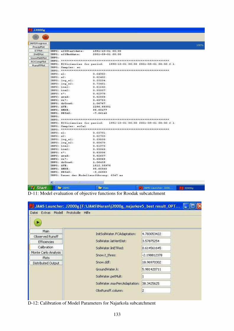
133
D-11: Model evaluation of objective functions for Roodak subcatchment
D-12: Calibration of Model Parameters for Najarkola subcatchment

134
D-13: Runoff Prediction of model for Najarkola subcatchment
D-14: Snowmelt simulation for Najarkola subcatchment

135
D-15: Snow Water Equivalent (SWE) simulation for Najarkola subcatchment

136
D-16: Model evaluvation of objective functions for Najarkola subcatchment

137
D-17: Calibration of Model Parameters for Naran subcatchment
D-18: Runoff Prediction of model for Naran subcatchment

138
D-19: Snowmelt simulation for Naran subcatchment
D-20: Snow Water Equivalent (SWE) simulation for Naran subcatchment

139
D-21: Model evaluvation of objective functions for Naran subcatchment

140
D-22: Calibration of model with global parameter set(gps) generated using area-weighted average of parameters for Roodak

141
D-23: Objective function results model after calibration of model using global parameter sets (gps) for Roodak
D-24: Calibration of model with global parameter set (gps) generated using area-weighted average of parameters for Najarkola

142
D-25: Objective function results model after calibration of model using global parameter sets (gps) for Najarkola

143
D-26: Calibration of model with global parameter set (gps) generated using area-weighted average of parameters for Naran
D-27: Objective function results model after calibration of model using global parameter sets (gps) for Naran

144
D-28: Start running the single HRU parameter model for SWE simulation in Shemshak station
D-29: Running the model using Monte Carlo Analysis Method for generation best parameter of SWE in various snow stations in the Latyan catchment

145
D-30: Calibration of SWE module for SWE simulation in the Shemshak snow station
D-31: SWE simulation using Single HRU in the Shemshak snow station

146
D-32: SWE simulation using Single HRU in the Ahar snow station
D-33: SWE simulation using Single HRU in the Garmabdar snow station

147
D-34: SWE simulation using Single HRU in the Konde Olya snow station
D-35: SWE simulation using Single HRU in the Lawasan snow station

Selbständigkeitserklärung
Ich erkläre, dass ich die vorliegende Arbeit selbständig und unter Verwendung
der angegebenen Hilfsmittel, persönlichen Mitteilungen und Quellen angefertigt
habe.
Jena, den 16.06.10 (Houshang Behrawan)