hydrostatics and stability prof. dr. hari v warrior...
TRANSCRIPT
Hydrostatics and Stability
Prof. Dr. Hari V Warrior
Department of Ocean Engineering and Naval Architecture
Indian Institute of Technology, Kharagpur
Module No. # 01
Lecture No. # 12
Hydrostatics Curves – II
In the last class, we talked about the TPC, TPI - that is the tonnes per centimeter
immersion and the tonnes per inch immersion - the amount of weight that needs to be put
to produce a centimeter of submersion of any body.
After this, we will now take a look at some other phenomenon that goes along with this;
this is known as the trimming.
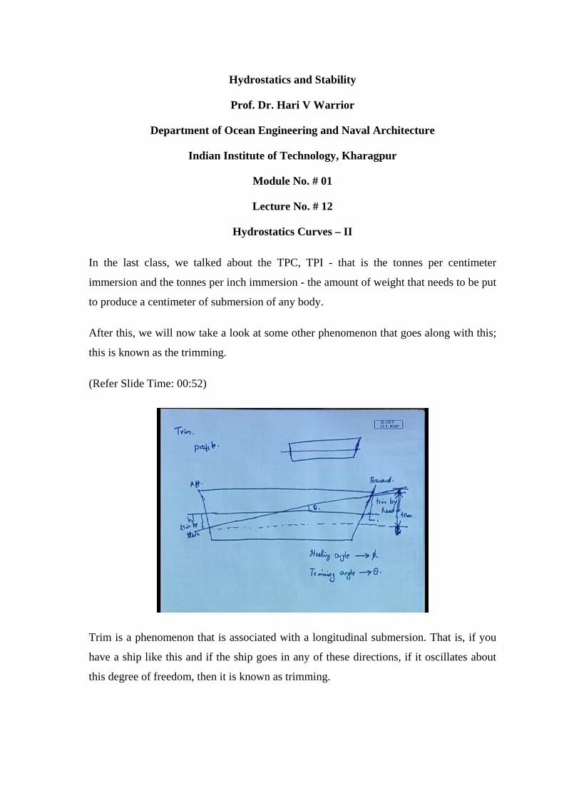
(Refer Slide Time: 00:52)
Trim is a phenomenon that is associated with a longitudinal submersion. That is, if you
have a ship like this and if the ship goes in any of these directions, if it oscillates about
this degree of freedom, then it is known as trimming.
The other one which we dealt about till now was about the ship; if this is the longitudinal
direction and if ship is made to oscillate in this fashion, it is known as heeling. So
heeling.
We are now going into trimming; the same way as you see heeling. That is, we have the
KG, KB, etcetera and the metacenter - the new position B phi. We discussed all that and
that is all seen through a transverse direction. That is, the view is from the transverse
direction. That is, if the ship is like this, we are seeing it from here. So, it is a transverse
view. Now, suppose, we see the same thing in a longitudinal direction - means like this;
we usually call it as a profile. So, we are seeing a ship like this.
This is another phenomenon that will occur in the ships. Now, instead of seeing this
metacenter, the center of buoyancy etcetera, in a transverse direction, we can also see the
same thing in the longitudinal direction. That is, if we are going to follow the same
principles between the transverse direction. The only thing is the difference between the
transverse direction and the longitudinal direction. Other than that all the principles
remain the same. There is a metacenter M, there is a center of buoyancy B 0 because of
the trimming, instead of heeling. Remember that we were talking about heeling in the
previous section. Instead of that, if the body starts trimming, because of the trimming,
there is a shift in the center of buoyancy like this. I will draw this figure. Let me draw it
better. This is the ship and this is its initial water line and because of its movement, it
causes it to trim like this.
So, this ship is now trimmed through an angle theta. I would like to mention that usually
heeling angle is denoted by phi and the trimming angle, which I have drawn there; this is
known as the trimming angle; the trimming angle is usually denoted by theta.
You have theta, the trimming of the ship and let us assume this is the forward side of the
ship and this is the aft side of the ship. We define it like this. This distance is known as
trim by head and this distance is known as by trim by stern.
The amount by which the front part trims from the main water line, there was an original
mean water line, the distance from which it trims the distance is known as trimming by
head and the aft side of the ship, the distance through it trims which is known aft that is
known as the trimming by the stern
So, we have this trimming and there is a slight ambiguity or vagueness about what you
really call as a trim. For example, trim can be this in this figure; this trimming by head,
can be called as a trim; trimming by stern can be called as trim or the whole distance
between the forward and the aft ward trim can be called as the trim itself. (Refer Slide
Time: 05:48) So, the distance between this distance and this distance can also be called
as the trim. To prevent the ambiguity in our course, we will define the total distance
between the forward top most part and the aft bottom most part, the distance between
those two, we will call it as the trim. This is the distance through which the ship has
totally tilted.
We now have the ship like this. As you can see, we always assume, but it is not really an
assumption, it is always true that the amount of ship that has gone down, that is, the
submerged part of the ship is equal to the emerged part of the ship. It is valid to some
extent and that principle we are assuming here.
So, trimming by stern is most likely to be equal to the trimming by the head. The trim by
stern and trim by head, both are almost equal in magnitude and therefore the total trim is
twice this value - twice the trim by head or twice the trim by stern; so, it is twice this.
That is what we will assume in our lectures.
This figure, I will keep here. Then this distance. Now for our purposes, let us do one
thing. Let us consider a rectangular barge. That is a barge with a rectangular shape. This
is a rectangular barge.
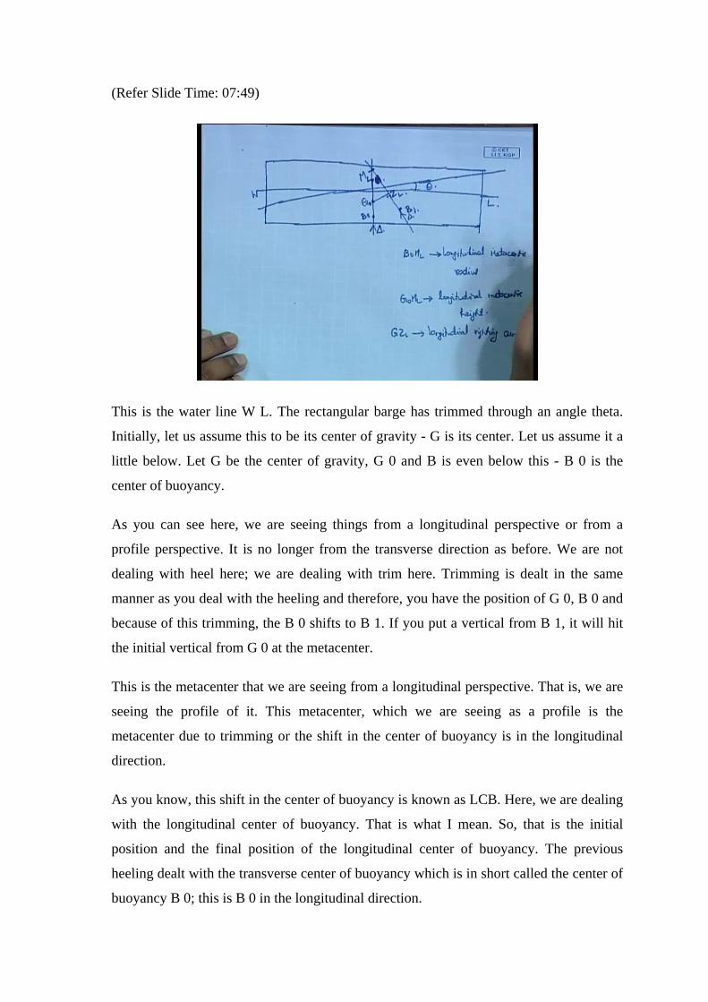
(Refer Slide Time: 07:49)
This is the water line W L. The rectangular barge has trimmed through an angle theta.
Initially, let us assume this to be its center of gravity - G is its center. Let us assume it a
little below. Let G be the center of gravity, G 0 and B is even below this - B 0 is the
center of buoyancy.
As you can see here, we are seeing things from a longitudinal perspective or from a
profile perspective. It is no longer from the transverse direction as before. We are not
dealing with heel here; we are dealing with trim here. Trimming is dealt in the same
manner as you deal with the heeling and therefore, you have the position of G 0, B 0 and
because of this trimming, the B 0 shifts to B 1. If you put a vertical from B 1, it will hit
the initial vertical from G 0 at the metacenter.
This is the metacenter that we are seeing from a longitudinal perspective. That is, we are
seeing the profile of it. This metacenter, which we are seeing as a profile is the
metacenter due to trimming or the shift in the center of buoyancy is in the longitudinal
direction.
As you know, this shift in the center of buoyancy is known as LCB. Here, we are dealing
with the longitudinal center of buoyancy. That is what I mean. So, that is the initial
position and the final position of the longitudinal center of buoyancy. The previous
heeling dealt with the transverse center of buoyancy which is in short called the center of
buoyancy B 0; this is B 0 in the longitudinal direction.
Similarly, this M that we see here is no longer designated as M; it is called as M L. So, B
0 M L is the longitudinal metacentric radius and G 0 M L is the longitudinal metacentric
height.
So, it shifts like this. (Refer Slide Time: 11:02) Then we can draw a perpendicular from
G 0 to this line; this is the perpendicular and we will call that Z L. As you remember,
before, we called G Z to be the righting arm; this is the restoring arm or this is the arm
which causes the ship to come back to its original position. In the same way, when the
ship trims, a restoring arm is produced again - a longitudinal restoring arm that is GZ L.
So, GZ L will represent the longitudinal righting arm. It is known as the longitudinal
righting arm and therefore, here at B 0 through this initial vertical, there is a horizontal
line delta, and through this there is a another force delta acting.
Here, you have the weight delta and in the final state, that is when the ship is trimmed,
you have the center of buoyancy here and through that center of buoyancy acts a force
delta that is equal to the weight of the ship because the ship is floating. So, delta the
weight of the ship acts upwards - that acts as the buoyancy force as it is called. The
buoyancy force acts upwards along B 1 in the vertical direction. (Refer Slide Time:
12:43) Between this and this, the vertical distance GZ L produces the righting arm and
because of this force and this righting arm, it produces what is called as righting moment.
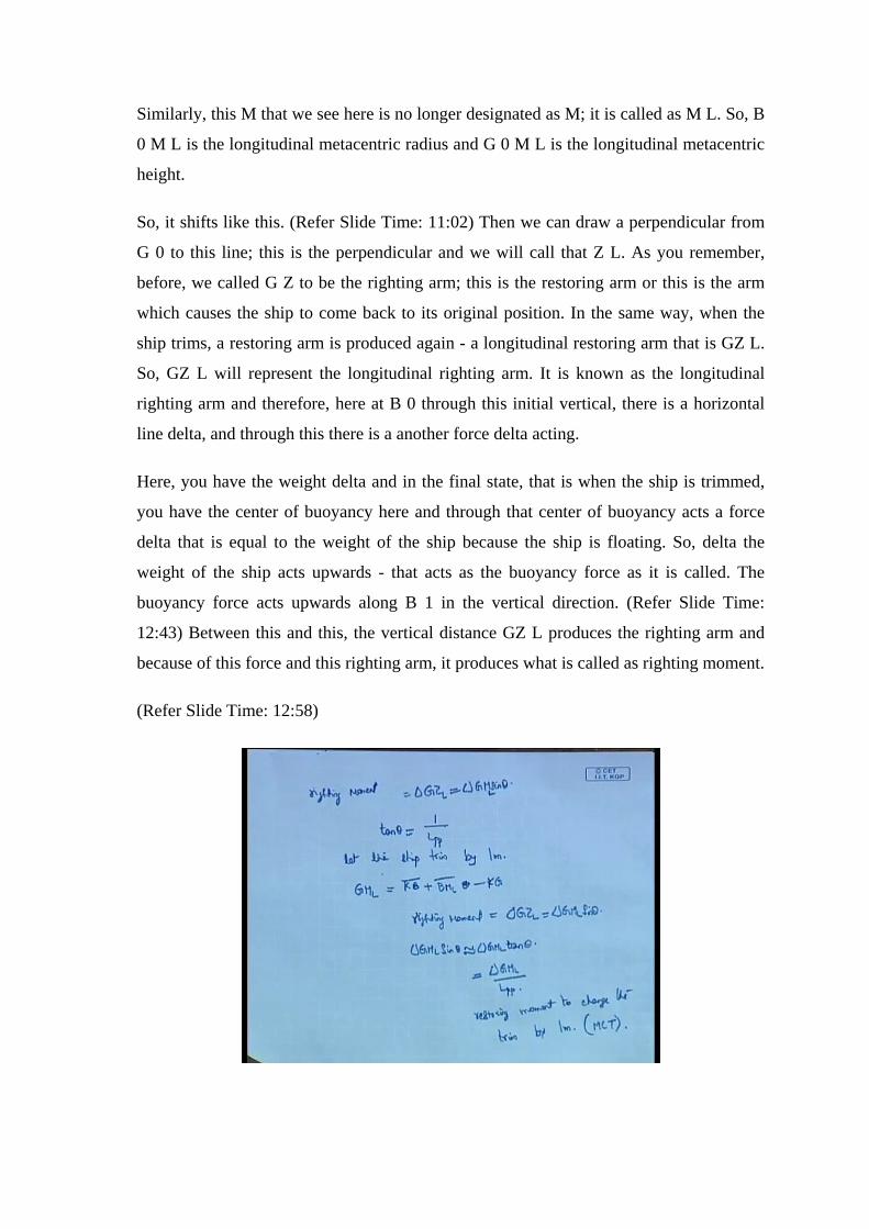
(Refer Slide Time: 12:58)
So, in this case, we get a righting moment which is given by GZ L into delta. It is equal
to delta into GM L sin theta. This is the same formula that you remember for heeling. We
discussed about the restoring arm and GZ and we talked about the restoring moment
delta into GZ and we have said that GZ is equal to GM sin phi for heeling; same
principle is holding here. delta GZ L is the longitudinal righting arm and delta GZ L is
equal to delta GM L sin theta.
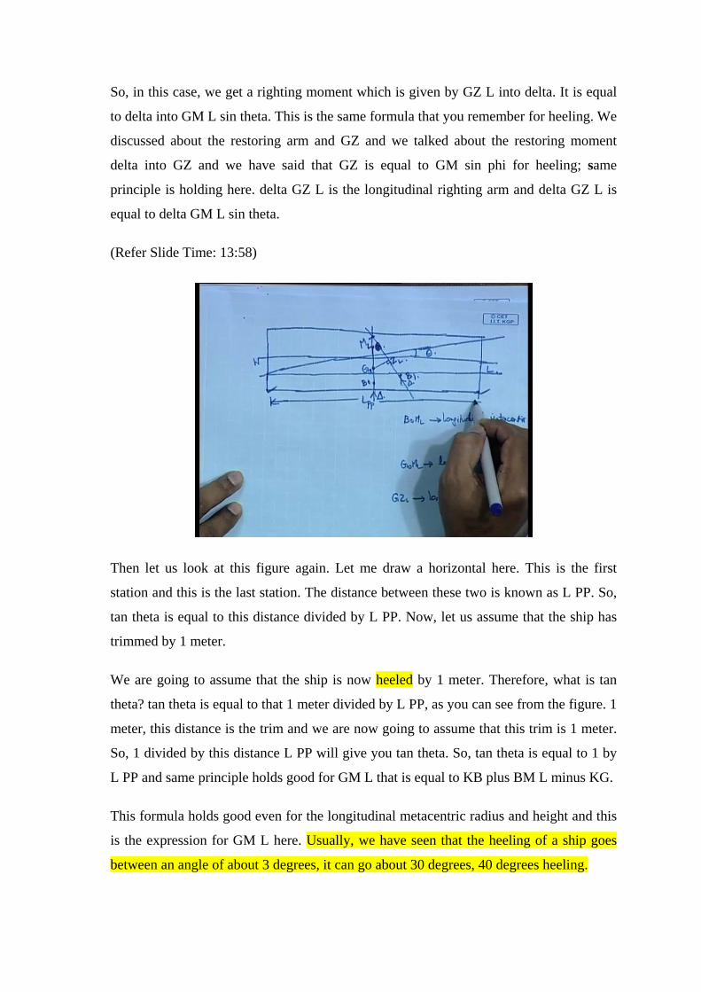
(Refer Slide Time: 13:58)
Then let us look at this figure again. Let me draw a horizontal here. This is the first
station and this is the last station. The distance between these two is known as L PP. So,
tan theta is equal to this distance divided by L PP. Now, let us assume that the ship has
trimmed by 1 meter.
We are going to assume that the ship is now heeled by 1 meter. Therefore, what is tan
theta? tan theta is equal to that 1 meter divided by L PP, as you can see from the figure. 1
meter, this distance is the trim and we are now going to assume that this trim is 1 meter.
So, 1 divided by this distance L PP will give you tan theta. So, tan theta is equal to 1 by
L PP and same principle holds good for GM L that is equal to KB plus BM L minus KG.
This formula holds good even for the longitudinal metacentric radius and height and this
is the expression for GM L here. Usually, we have seen that the heeling of a ship goes
between an angle of about 3 degrees, it can go about 30 degrees, 40 degrees heeling.

For trimming, we do not encounter such large angles because mainly in the other case,
we are looking at the breadth of the ship as the denominator of tan theta whereas, in this
case we are looking at the length of the ship as the denominator, which is very large; as a
result of which, the tan theta is very small.
We can assume that the righting moment is equal to delta GZ L equals delta GM L sin
theta and delta GM L sin theta is approximately equal to delta GM L tan theta. We have
seen here, tan theta is equal to 1 by L PP; that is equal to delta GM L by L PP. This
expression gives you the restoring moment to change the trim by 1 meter and this is
known as MCT. This is a very important term. In many places, you will find the
application of this coming up; this is known as MCT, the moment to change the trim by
1 meter.
So, this is some definition about trim. We will have to do more about trim and the
longitudinal metacentric height. and all that in a later lecture we will be doing about it.
Then let us talk about a couple of important parameters that we have discussed so far.
(Refer Slide Time: 18:22)
The first of which, is the trim by head. This the first important thing that we learned in
previous few lectures, trim by head and then we have trim by stern. Then volume of
displacement - this we know what it is, we have all described it many times. Then LCB -
LCB is the longitudinal center of buoyancy.
So, this is another parameter that we discussed about. Then we talked about LCF. This is
known as the longitudinal center of floatation; longitudinal center of floatation is the
centroid of the water plane area and we have discussed it.
This is known as the LCF. Then we talked about moment to change the trim by 1 meter –
MCT, this is another important term. Then we have KM, which is the distance between
the keel and the metacenter. Then C B - this is the block coefficient. Then a couple of
other coefficients like C M, C W etcetera - the water plane area coefficient, the mid-ship
section area coefficient and so on.
These are some important terms that we have discussed so far and K B another one is K
B; it is the vertical center of buoyancy.
These things are known as hydrostatic particulars or it is known as hydrostatic data. Note
that all the details of the ship do not come under the category of hydrostatic data. Only
these terms will come under the category of hydrostatic data. These hydrostatic data are
some of the particulars of the ship itself. It has not got anything to do with the loading;
even though, some transfer in loading can produce some changes in this. The G factor,
the KG or GM do not come under the category of hydrostatic data; we do not call them
by that name.
(Refer Slide Time: 21:49)

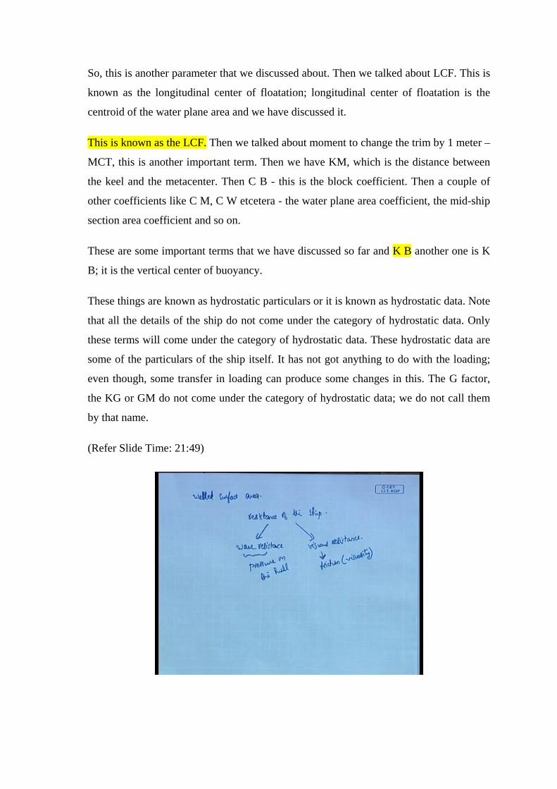
So, next There is another term, which we use commonly and this is known as the wetted
surface area. Wetted surface area means the total area of the ship that is subjected to
water. So, total part of the ship that is wet is known as wetted surface area.
If you have the ship like this, the whole region that is wetted is known as the wetted
surface area.
Then we come to wetted surface area Why the wetted surface area is important? There
are a couple of parameters that depend upon the wetted surface area. They are mainly,
the resistance of the ship. that is Just to give you a quick review of resistance. This is
another course, resistance and propulsion in which you will be doing things in greater
detail, but here I will just mention some of the details of resistance.
So, the resistance of the ship is really divided into two types of resistances: one is known
as the wave resistance and the other is known as the viscous resistance.
These are two types of resistance. One is the wave resistance and this is due to the
pressure on the hull. The wave resistance is due to the pressure on the hull and viscous
resistance is due to the friction or viscosity.
These are two types of resistances you encounter in ships. The wave resistance depends
upon the form of the ship. It defines the pressure distribution along the hull of the ship.
and this pressure distribution. For example, a pressure difference can produce a force.
So, there will be a high pressure on the forward part of the ship and there will be a low
pressure on the aft part of the ship and therefore, there will be a force acting from the
forward to the backward side, which is the resistance that the ship encounters while it
moves forward. This is known as the wave resistance. This generates waves in a
particular form in the back of the ship and they are known as Kelvin wave form and the
other resistance is the viscous resistance, which is the frictional resistance.
The frictional resistance is also important and depending upon the type of ship that you
have, one resistance or the other resistance will predominate. Very large ships like
container ships and oil tanks usually have a very high viscous resistance.
So, that is about the wetted surface area of the ship. That is, the amount of ship that is
subjected to the wetting. Then we come to what is known as the hydrostatic curves.
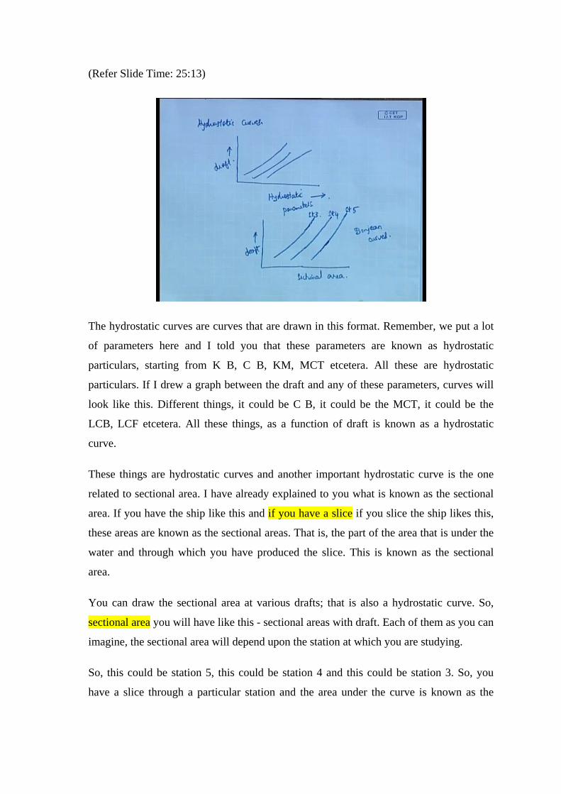
(Refer Slide Time: 25:13)
The hydrostatic curves are curves that are drawn in this format. Remember, we put a lot
of parameters here and I told you that these parameters are known as hydrostatic
particulars, starting from K B, C B, KM, MCT etcetera. All these are hydrostatic
particulars. If I drew a graph between the draft and any of these parameters, curves will
look like this. Different things, it could be C B, it could be the MCT, it could be the
LCB, LCF etcetera. All these things, as a function of draft is known as a hydrostatic
curve.
These things are hydrostatic curves and another important hydrostatic curve is the one
related to sectional area. I have already explained to you what is known as the sectional
area. If you have the ship like this and if you have a slice if you slice the ship likes this,
these areas are known as the sectional areas. That is, the part of the area that is under the
water and through which you have produced the slice. This is known as the sectional
area.
You can draw the sectional area at various drafts; that is also a hydrostatic curve. So,
sectional area you will have like this - sectional areas with draft. Each of them as you can
imagine, the sectional area will depend upon the station at which you are studying.
So, this could be station 5, this could be station 4 and this could be station 3. So, you
have a slice through a particular station and the area under the curve is known as the
hydrostatic curve. This sectional area curve Such curves dealing with the sectional area
are known as Bonjean curves; the word used is Bonjean curves.
Sometimes, usually you draw different of these curves that are at different stations,
starting from station 0; for an instance, the aft station 0, 1, 2, 3, 4, 5 like that. We can
draw the Bonjean curves for different stations and this will produce another curve the
whole curve is known as a Bonjean set. So, this Bonjean set will give you the Bonjean
curves at different points or different stations.
(Refer Slide Time: 29:11)
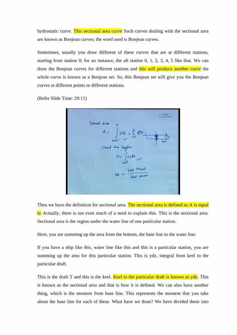
Then we have the definition for sectional area. The sectional area is defined as A is equal
to Actually, there is not even much of a need to explain this. This is the sectional area.
Sectional area is the region under the water line of one particular station.
Here, you are summing up the area from the bottom, the base line to the water line.
If you have a ship like this, water line like this and this is a particular station, you are
summing up the area for this particular station. This is ydz, integral from keel to the
particular draft.
This is the draft T and this is the keel. Keel to the particular draft is known as ydz. This
is known as the sectional area and that is how it is defined. We can also have another
thing, which is the moment from base line. This represents the moment that you take
about the base line for each of these. What have we done? We have divided these into
different delta Ts and that is what dz stands for - different delta Ts. If I had to write this,
it will become sigma n equals 1 to some capital N of y i delta T where delta T into alpha,
where you have the Simpsons multiplier.
So, alpha i into delta T where delta T is the distance between the different water lines.
So, the moment from the baseline is known as M equals from keel to T, z into y dz. This
is known as the sectional area as a function of draft. This is known as the moment from
the base line. Moment from the baseline is zydz.
(Refer Slide Time: 31:49)
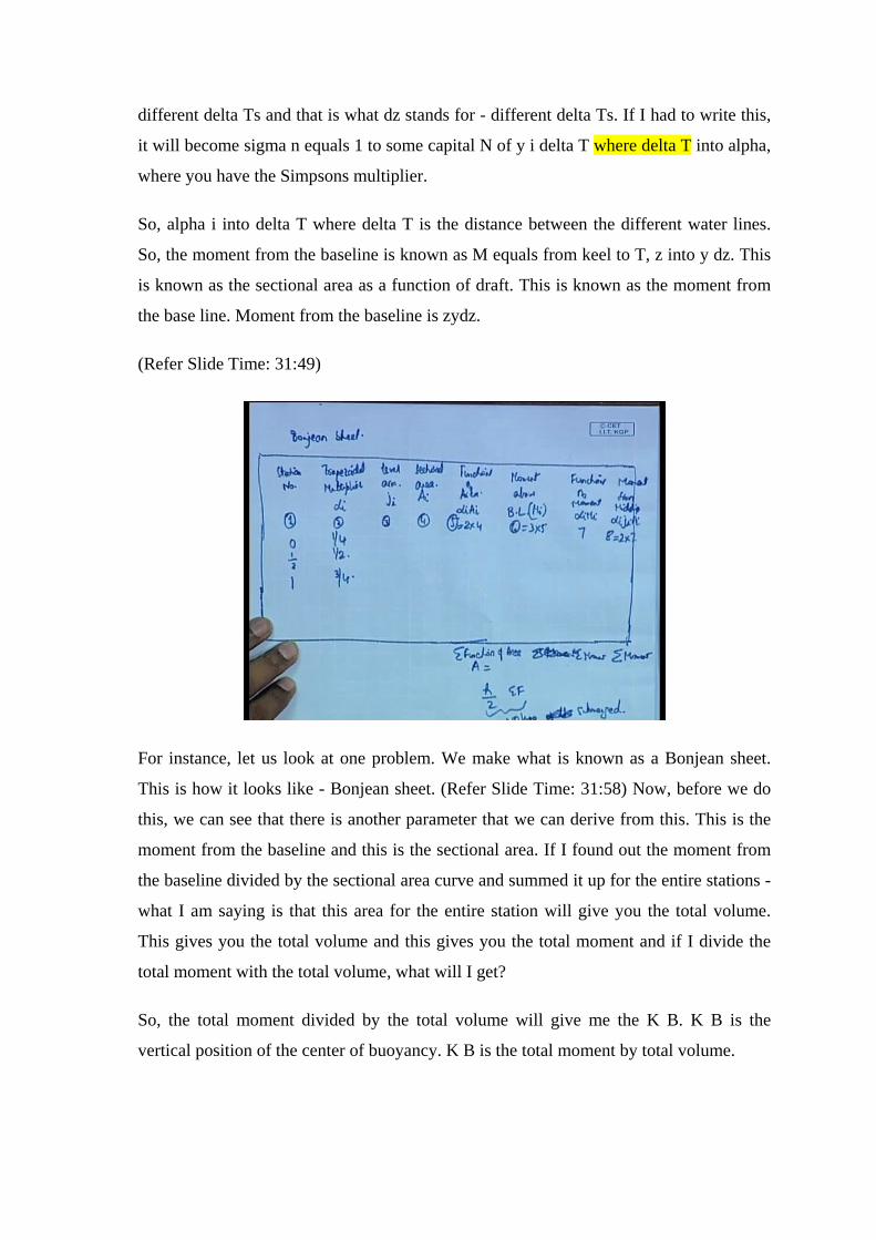
For instance, let us look at one problem. We make what is known as a Bonjean sheet.
This is how it looks like - Bonjean sheet. (Refer Slide Time: 31:58) Now, before we do
this, we can see that there is another parameter that we can derive from this. This is the
moment from the baseline and this is the sectional area. If I found out the moment from
the baseline divided by the sectional area curve and summed it up for the entire stations -
what I am saying is that this area for the entire station will give you the total volume.
This gives you the total volume and this gives you the total moment and if I divide the
total moment with the total volume, what will I get?
So, the total moment divided by the total volume will give me the K B. K B is the
vertical position of the center of buoyancy. K B is the total moment by total volume.

Similarly, you can make the Bonjean sheet like this. You have the station number, then
trapezoidal multiplier, lever arm, sectional area A i, lever arm j i, trapezoidal multiplier
alpha i, then functions of the area alpha i A i, then moment above base line that is M i,
then functions of moment above the baseline alpha i M i and then you can also have one
more, you can have the moment from mid-ship alpha i j i A i.
So, the moment from midship So, this is 1 this is 2, 3, 4, what is 5? 5 is equal to 2 into 4,
6 equals 3 into 5, 7, 8 equals 2 into 7.
So, 0, half. This is how they have made the stations. This has nothing to do with the
problem as such, that is, the way in which the problem is solved. It is just the way in
which, they have solved it. It means they have a station at 0, they have a station at half.
You know what are these? They are half ordinates.
So, you have a station at half, then you have the next station at 1, 1 and half, 2, like this.
So, half, 1 and the corresponding trapezoidal multiplier which we have done will come
later as 1 by 4, 1 by 2, 3 by 4 like that. Lever arm, as you see, this is the lever arm from
the initial station. So, the lever arm can be taken in two ways: one is you can always take
the lever arm from the station 0. You put the station 0 as 0 then 1, 2, 3, 4, 5, like that or
you can have the mid-ship as lever 0 and one side to the forward as positive and one side
to the aft as negative; so, that is another possibility.
So you have like this and area equals, when you do this, sigma function of area, this is
sigma moment and this is sigma moment again. Not this one, this one. Sorry, this is
sigma moment one and this is another sigma moment. These are two moments: one is the
moment taken from the baseline; moments of each of the areas above the baseline and
the other one is the moment of the different stations.
So, this is known as a Bonjean sheet and using such sheets, you can always calculate the
total volume from this - by multiplying h by 2 with sigma function of area, you will get
the total volume, volume of the underwater portion or volume submerged. you will get
the volume submerged and What is the use of the sigma moment from the baseline?

(Refer Slide Time: 38:26)
The sigma moment from the baseline divided by sigma function of area will give you the
KB.
So, this gives you the KB and similarly, the sigma moment from station 0 divided by
sigma function of area will give you the LCB, the longitudinal center of buoyancy. This
holds good and in this way, you can calculate LCB and the KB for such ships.
So, you can find the volume, you can find the LCB and you can find the KB; all of that is
possible from a Bonjean sheet. You can see the important of the Bonjean sheet. Most of
you, who will go into the naval architecture career in ship yards or consultancy company,
they will be doing a lot of these Bonjean sheet work. You will have to definitely
calculate the volume submerged and the LCB, KB etcetera you will have to find out.
(Refer Slide Time: 40:17)
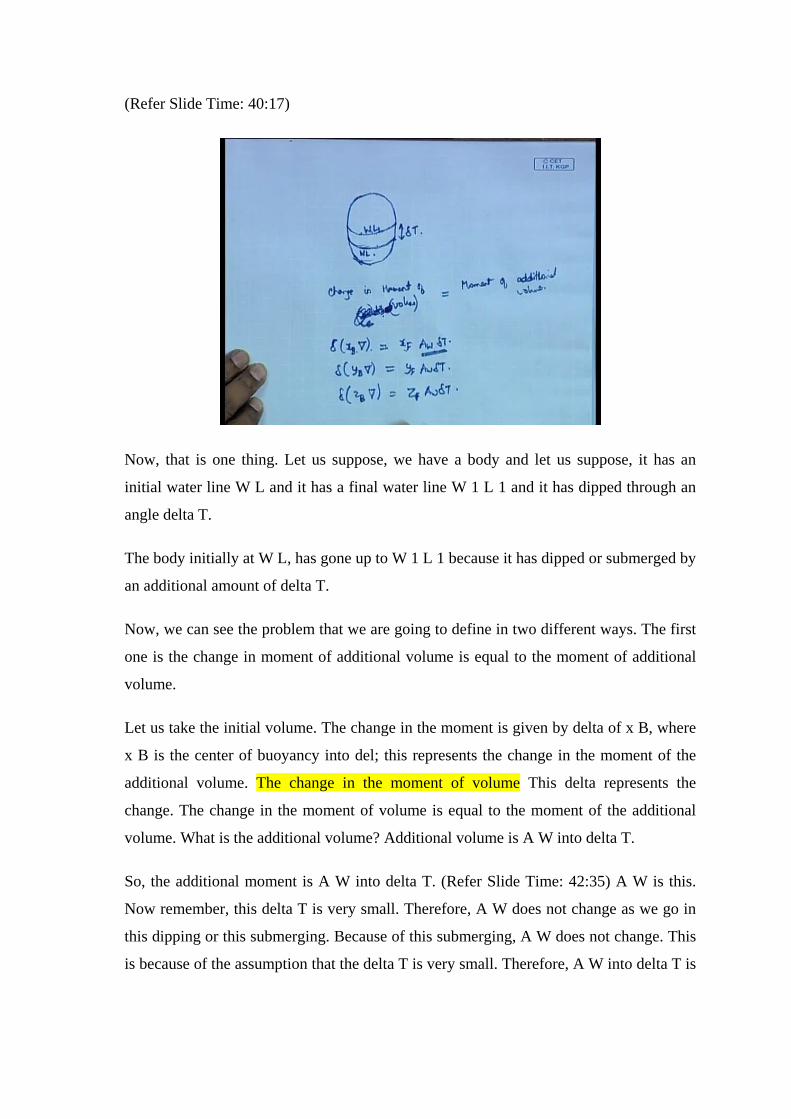
Now, that is one thing. Let us suppose, we have a body and let us suppose, it has an
initial water line W L and it has a final water line W 1 L 1 and it has dipped through an
angle delta T.
The body initially at W L, has gone up to W 1 L 1 because it has dipped or submerged by
an additional amount of delta T.
Now, we can see the problem that we are going to define in two different ways. The first
one is the change in moment of additional volume is equal to the moment of additional
volume.
Let us take the initial volume. The change in the moment is given by delta of x B, where
x B is the center of buoyancy into del; this represents the change in the moment of the
additional volume. The change in the moment of volume This delta represents the
change. The change in the moment of volume is equal to the moment of the additional
volume. What is the additional volume? Additional volume is A W into delta T.
So, the additional moment is A W into delta T. (Refer Slide Time: 42:35) A W is this.
Now remember, this delta T is very small. Therefore, A W does not change as we go in
this dipping or this submerging. Because of this submerging, A W does not change. This
is because of the assumption that the delta T is very small. Therefore, A W into delta T is

the additional volume and where does this additional volume act? The additional volume
always acts at the centroid of this water line.
So, the centroid of the water plane area or the centroid of that water line area is known as
the center of flotation, x F. So, x F into A W delta T will give you the moment due to the
additional volume.
(Refer Slide Time: 43:37) There is a slight difference between this and this. The
difference is that this is the additional volume. Additional volume into where it is acting,
x F is the moment due that additional volume. This is the change in the moment itself. It
is the change in the moment of the volume.
So, that moment of the volume is what? the volume itself acts We can assume that the
total volume underneath acts at x B. x B is the longitudinal center of buoyancy. So, the
total volume of the ship acts at x B and therefore, x B into del gives you the moment of
the ship. Now, the change in the moment will be delta of that. So, the change in the
moment of the volume Let me remove this, it is confusing.
If I write it like this, it is better. Change in the moment of volume is equal to moment of
additional volume. So, you get this concept. Similarly, you will have delta of y B into del
equals y F A W delta T; delta of z B into del equals z F into A W delta T.
(Refer Slide Time: 45:13)
You have three formulas here. Now, we can expand this. This is a product of two terms.
You know that you can expand the derivative of the product of two terms. That will give
you delta into delta x B plus x B into delta of del is equal to x F into A W into delta T,
del of delta y B plus y B into delta del equals y F into A W into delta T and del of delta z
B plus z B into delta of del equals z F into A W into delta T.
So, this gives you some terms. Now, dividing by delta del equals A W delta T. If you do
some manipulations, this reduces to x F minus x B is equal to d of x B by dT del by A W
and y F minus y B equals d of y B by d T into del by A W.
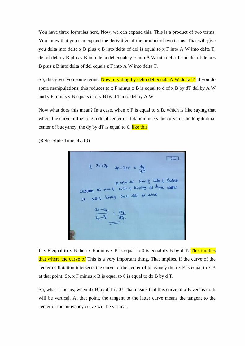
Now what does this mean? In a case, when x F is equal to x B, which is like saying that
where the curve of the longitudinal center of flotation meets the curve of the longitudinal
center of buoyancy, the dy by dT is equal to 0. like this
(Refer Slide Time: 47:10)
If x F equal to x B then x F minus x B is equal to 0 is equal dx B by d T. This implies
that where the curve of This is a very important thing. That implies, if the curve of the
center of flotation intersects the curve of the center of buoyancy then x F is equal to x B
at that point. So, x F minus x B is equal to 0 is equal to dx B by d T.
So, what it means, when dx B by d T is 0? That means that this curve of x B versus draft
will be vertical. At that point, the tangent to the latter curve means the tangent to the
center of the buoyancy curve will be vertical.

So, this is an interesting and useful derivation which we will be using in some places. So,
where the center of floatation intersects the center of buoyancy, the tangent to the latter
curve that is, the center of buoyancy curve will be vertical.
Then if you do a little more mathematics, x F minus x B divided by z F minus z B is
equal to dx B by dz B. That is, I just divided 1 from the other. This is just use like that in
some places x F minus x B divided by z F minus z B is equal dx B by dz B is another
formula that is used in some places.
So, there is an LCB curve and there is an LCF curve and when you draw them together
in the draft, it will be like this.
(Refer Slide Time: 50:12)
Now, draft will be here. You have the draft and here you have the LCB curve and LCF
curve. One curve is like this and another curve is like this. So, at that point, if this is the
LCB curve, the tangent to the curve will be vertical.
So, this interesting derivation, you should take home today. So, with that I will stop
today’s lecture.
Thank you.