Hyperbolic Constructions in

Geometer’s Sketchpadby Steve Szydlik

December 21, 2001

1 Introduction – Non-Euclidean Geometry

Over 2000 years ago, the Greek mathematician Euclid compiled all of the known geometryof the time into a 13-volume text known as the Elements. In itself, that was an impressivefeat, but what made his efforts particularly astonishing was that he laid a logical foundationfor the subject as well. He established five axioms for geometry, then showed that everyresult in his text could be proven from those axioms.

In modern language, Euclid’s postulates can be stated as follows:

I. For every point P and every point Q not equal to P there exists a unique line ` thatpasses through P and Q.

II. For every segment AB and every segment CD there exists a unique point E such thatB is between A and E and segment CD is congruent to segment BE.

III. For every point O and every point A not equal to O, there exists a circle with centerO and radius OA.

IV. All right angles are congruent to each other.

V. For every line ` and point P that does not lie on `, there exists a unique line m throughP that is parallel to `.

From the time the Elements was published, Euclid’s axioms have been the subject ofcareful scrutiny, criticism and controversy. Modern texts note several deficiencies in theaxioms (see, for example [3], [1]). Generally speaking, Euclid’s axioms are not precise enough,and in his text, Euclid relies on diagrams and makes use of unstated assumptions. Manymathematicians, Hilbert in particular (see [2]), have devoted themselves to placing geometryon a firmer foundation than did Euclid. Nevertheless, Euclid’s axioms form the basis ofEuclidean geometry, the plane geometry studied by most high school students today.

In spite of some of the weaknesses of Euclid’s axioms, they were, for the most partaccepted by other mathematicians. For example, Axiom I tells us that through any twopoints, one and only one line can be drawn. Most people would grant that statement as atruth about our physical world. So it is with Euclid’s first four axioms. However, the fifthand final axiom proved extremely controversial.

Although Euclid’s fifth axiom, called the “parallel postulate”, seems a reasonable as-sumption, geometers were skeptical from its first appearance. Specifically, many thoughtthat Euclid V could be proven from his other four axioms. If this were true, there wouldbe no need to assume it, and Euclid would have needed only four axioms for his Elements.For 2000 years, geometers attempted to prove the “parallel postulate” and met with utter

1

failure. In every purported proof, there could be found a flaw, some statement which in turncould not be proven.

In the 19th century, mathematicians began to look at the postulate in a new way. Ratherthan trying to prove Euclid V, they began to question whether such attempts could reallysucceed. Three mathematicians (Gauss, Bolyai, and Lobachevsky) independently developeda noncontradictory geometry in which the parallel postulate is false. One way that Euclid’sfifth axiom can fail is to have “too many parallel lines through a point”:

There exists a line ` and a point P not on ` such that at least two distinct lines parallelto ` pass through P .

Rather than assuming the parallel postulate, the three men assumed this axiom, whichis today called the Hyperbolic Axiom. Using the hyperbolic axiom and Euclid’s otherfour postulates, Gauss, Bolyai, and Lobachevsky developed the important and rich subjectwhich has come to be known as hyperbolic geometry.

Before discussing models on hyperbolic geometry, we must point out that the hyperbolicaxiom is not the only way in which Euclid V can fail. It is possible, of course, that there are“not enough parallel lines through a point”:

There exists a line ` and a point P not on ` such that there are no lines parallel to `which pass through P .

If we assume this axiom, called the Elliptic Axiom, rather than Euclid’s parallel postulate,we obtain yet another type of geometry, albeit with some restrictions. Elliptic geometryrequires slight modifications to the other axioms of geometry and will not be consideredhere. Non-Euclidean geometry consists of both elliptic and hyperbolic geometry, thoughin the context of this report it will generally refer to hyperbolic geometry.

2 Models of Hyperbolic Geometry

One particular difficulty with non-Euclidean geometry is visualization. How can one un-derstand a universe in which the parallel postulate does not hold? In our experience, if weconstruct two parallel lines, then draw a third line which intersects one of the two parallellines, it seems clear that it must intersect the other. The solution to this difficulty againrequires a change in thinking. We abstract our notions of common geometric terms such as“line”, “point”, and “congruent”, reinterpret them and create a universe, or model, whereEuclid’s first four axioms hold, but the fifth one doesn’t.

There are many models of hyperbolic geometry. Perhaps the best known are the Poincaredisk model, the Poincare half-plane model, and the Beltrami-Klein (or Klein) model. Ineach of these models there are different interpretations of undefined geometric terms suchas “point,” “line,” and “congruent.” In the non-Euclidean models, the interpretations aregenerally different from their usual Euclidean notions, so standard Euclidean constructionsdo not directly apply. For example, in the Poincare models, “lines” are generally (butnot always) interpreted to be arcs of circles, so in these models, lines cannot generally beconstructed with just a Euclidean straightedge.

2

The non-Euclidean models thus provide a challenge: how does one construct typicalgeometric objects in hyperbolic geometry? With a straightedge and compass, one can drawcircles, bisect angles, and construct midpoints in Euclidean geometry. Using the same tools,how does one perform the same constructions in the hyperbolic models?

Alexander and Finzer have written Geometer’s Sketchpad scripts to perform ten typicalconstructions in the Poincare disk model. The constructions are available at

http://mathforum.org/sketchpad/maa96/alexander/index.html

and include scripts to

1. Construct a non-Euclidean line, given two points on the line.

2. Construct a non-Euclidean line segment, given the endpoints of the segment.

3. Measure the length of a non-Euclidean line segment.

4. Calculate the measure of an angle.

5. Construct the bisector of a given angle.

6. Construct a perpendicular to a given line through a given point on the line.

7. Construct a perpendicular to a given line through a given point not on the line.

8. Construct the perpendicular bisector of a non-Euclidean line segment.

9. Construct a circle, given its center and a point on the circle.

10. Construct a circle, given its center and two points determining the radius of the circle.

These constructions use the Euclidean tools of Geometer’s Sketchpad, which are, in essence,computer versions of the straightedge and compass. (It should be noted that items #3 and#4 above are not actually constructions, since they require the notion of measurement.)

In this document, we describe the steps necessary to perform Constructions 1–10 forthe other two well-known models of hyperbolic geometry, the Beltrami-Klein and Poincarehalf-plane models. The descriptions provide a context for understanding the constructions inassociated Geometer’s Sketchpad scripts for these models. In addition, creating a script forone of these “standard” constructions occasionally necessitated the development of relatedtool which is useful in itself. For example, constructing the perpendicular bisector of a linesegment in the model involves finding the “pole” of a Klein line, so the tool kpole.gss wasdeveloped for that purpose. These additional constructions are described as well when theyarise, but the list of such additions includes scripts which find the midpoint of a line segment(kmidpt.gss and phmidpt.gss) and find the reflection of a point about a line (kreflpt.gss andphreflpt.gss), and scripts which map points in the Klein disk to their respective points inthe Poincare disk (kd_to_pd.gss) and back (pd_to_kd.gss) under the isomorphism betweenthe models. Finally, since a circle (i.e. the set of points a given distance from a given point)in the Klein disk is not a Euclidean circle, the Klein tools for constructions #9 and #10result in loci of points, due to limitations of Geometer’s Sketchpad. This creates additional

3

difficulties when one wishes to attempting perform geometric operations on Klein circles(such as finding the intersection of two Klein circles); The current version of Sketchpad isunable to find the intersection of two objects which are defined as loci. As a result, tools arealso given which will find the intersection of two circles (kintcirc.gss), find the intersectionpoint(s) of a Klein circle with a Klein line (kintlncr.gss), and find the intersection point(s)of a Klein circle with a Klein segment (kintsgcr.gss). Please note that for all the tools, theconstructions are only described - formal proofs of correctness are omitted.

The ten Klein scripts are provided first, followed by the half-plane scripts. To the best ofour knowledge, the Klein scripts are original. That is, though others have certainly demon-strated the same constructions, they are an original compilation in the form of Sketchpadscripts. The same may be said for constructions 5–10 in the Poincare half-plane model.Bennett has created scripts for constructions 1–4 for the half-plane model. His scripts maybe found at

http://www.keypress.com/sketchpad/misc/sibley/sibley.htm.

Peil has also written several scripts for the half-plane model, which may be found at

http://classweb.mnstate.edu/peil/Projects/geo.html.

Although several of the constructions described here appear to duplicate Peil’s work, thereare some differences. For example, the midpoint and circle constructions described here useonly straightedge and compass constructions, while Peil’s scripts involve coordinate geometryas well.

3 Beltrami-Klein Model Scripts

In the Beltrami-Klein model of non-Euclidean geometry, we fix a Euclidean circle γ. “Points”in this model are interpreted to be points interior to γ, and “lines” are interpreted to beeither open chords of the circle (i.e. chords without their endpoints) or open diameters ofthe circle. The Klein model is neither isometric nor conformal; that is, it represents neitherdistances nor angle measures faithfully. However, the model does provide several distinctadvantages over the Poincare models. First, it is immediately apparent that the hyperbolicaxiom holds in this model. Given a chord ` of γ and a point P interior to the circle that isnot on the chord, there are an infinitude of distinct chords passing through P which do notintersect `. Second, although the model is not conformal, constructing perpendicular linesin the Klein disk proves to be somewhat easier than in the Poincare models.

Each construction described below corresponds to an available Geometer’s Sketchpadscript. The name of the associated script is given in bold-face next to the number of theconstruction. In Sketchpad, the script tools assume that one is performing the constructionsusing a fixed circle labelled “Klein Disk,” defined by a center labelled “K-Disk center,” anda point on the circle labelled “K-Disk radius.” The Sketchpad file “klnstrt.gsp” contains thisstartup figure. The simplest way to use the Klein tools is to create a directory, perhaps called“klein,” in which all the scripts and “klnstrt.gsp” is stored. Set the script tool directory inSketchpad to be “klein,” and the tools will be accessible from the Sketchpad desktop.

4

For the Klein constructions discussed below, Greenberg [1] provides much useful back-ground. Stahl’s text [4] discusses the Klein model in depth as well. Note also that in theconstructions, only the most general cases are considered. For example, if one wants toconstruct a perpendicular to a general Klein line, Constructions #6 and #7 will work nicely.However, if the Klein line happens to be a diameter of the Klein disk, the constructionwill fail. As noted in the introduction, in addition to the standard ten constructions, weinclude constructions which find the midpoint of a Klein segment (see item #8(i) below)and the reflection of a point about a Klein line (see item #9(i)). The pole of a Klein lineis a useful construction in this model, and a description of that construction is also given(see item #5(i)). Throughout the constructions, we will use terms such as “K-line” and“K-circle” as shorthand for “Klein line” and “Klein circle”. This will distinguish betweenthe non-Euclidean constructions and their Euclidean counterparts.

1. (kline.gss) Construct a Klein line, given two points on the line.

Given: Two points A and B inside the Klein disk.

To Construct: K-line←→AB, i.e. the Euclidean chord of the Klein disk which passes

through A and B.

a) Construct the Euclidean line←→AB.

b) Let P and Q be the points of intersection of←→AB with γ. (P and Q are ideal

points.)

c) Construct Euclidean segment PQ. By definition, this segment (excluding end-points P and Q) is the K-line passing through A and B.

2. (ksegmnt.gss) Construct a Klein line segment, given the endpoints of the segment.

Given: Two points A and B inside the Klein disk.

To Construct: K-segment AB.

a) Construct the Euclidean segment AB. By definition, this is also the K-segmentjoining A and B.

3. (klength.gss) Measure the length of a Klein line segment.

Given: Two points A and B inside the Klein disk.

To Measure: The K-length of segment AB.

a) Construct the K-line←→AB. Let P and Q be the ideal points of this K-line, i.e. the

ends of this chord of γ passing through A and B.

b) Find each of the following Euclidean lengths: AP , AQ, BP , BQ.

5

Q

PBA

Figure 1: Calculating the length of a line segment AB in the Klein model.

c) Define the cross-ratio (AB, PQ) by

(AB, PQ) =AP/AQ

BP/BQ.

Let d = 12· |`n(AB,PQ)|. Then d is the K-length of segment AB. (See [1,

Theorem 7.4].) d is independent of the labelling of P and Q (i.e. their labellingcould be reversed without affecting d). See Figure 1.

Note: Length is defined as one-half the absolute value of the natural log of the rel-evant cross-ratio. One could use a different log base or delete the factor of 1

2. The

result would still be a perfectly legitimate hyperbolic measure of length. However, ourparticular choice of distance allows for simpler relationships between lengths and anglemeasures in hyperbolic trigonometry. Specifically, this choice yields the constant k = 1in Theorems 10.1 and 10.2 of [1], and allows for direct use of the hyperbolic law ofsines and law of cosines ([1, Theorem 10.4]).

4. (kangmea.gss) Calculate the K-measure of an angle.

Given: Klein points A, B, and C.

To Calculate: the K-measure of 6 ACB.

a) Construct triangle ∆ACB. Note that constructing the triangle in the Klein diskis the same as constructing it in the Euclidean sense.

b) Let a be the length of side BC, the side opposite 6 A. Let b be the length of sideAC, the side opposite 6 B. Let c be the length of side AB, the side opposite 6 C.Lengths should be measured using the “standard Klein unit.” See Construction#3 above.

6

n

m

l

P(l)

R

Q

O

Figure 2: Constructing the pole P (`) of line ` in the Klein model.

c) According to the hyperbolic law of cosines (See [1, Theorem 10.4])

cosh c = cosh a cosh b− sinh a sinh b cos C.

Thus

C = arccos

(cosh c− cosh a cosh b

− sinh a sinh b

).

5. i) (kpole.gss) Construct the pole of a given K-line (see [1, p. 239]).

Given: K-line `.

To Construct: P (`), i.e. the intersection of the tangents to the defining K-circleγ at the endpoints of the Euclidean chord making up `.

a) Let Q and R be the endpoints of the Euclidean chord which constitutes K-line`.

b) Draw segments OQ and OR, where O is the center of γ.

c) Construct the Euclidean line m through Q which is perpendicular to OQ.Construct the Euclidean line n through R which is perpendicular to OR. Byconstruction, m and n are the tangents to γ through the points Q and R,respectively.

d) Assuming ` is not a diameter of γ, lines m and n intersect at a point P (`)exterior to γ.

P (`) is the pole of `. See Figure 2.

ii) (kangbis.gss) Construct the bisector of a given angle.

Given: Klein points A, B, and C.

To Construct: the angle bisector of of 6 ACB.

(Greenberg outlines this construction in [1, p. 273].)

7

Q

R

P

D

E

A

CB

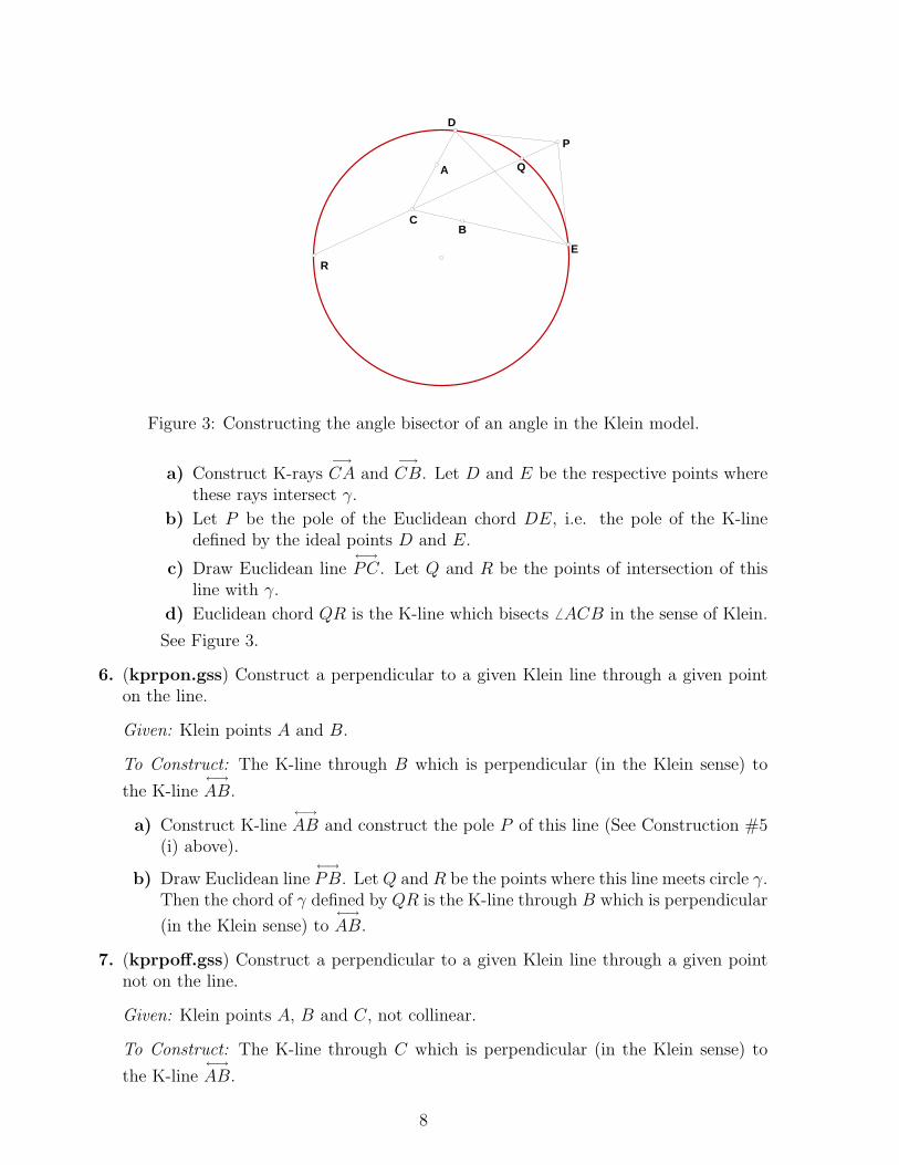
Figure 3: Constructing the angle bisector of an angle in the Klein model.

a) Construct K-rays−→CA and

−→CB. Let D and E be the respective points where

these rays intersect γ.

b) Let P be the pole of the Euclidean chord DE, i.e. the pole of the K-linedefined by the ideal points D and E.

c) Draw Euclidean line←→PC. Let Q and R be the points of intersection of this

line with γ.

d) Euclidean chord QR is the K-line which bisects 6 ACB in the sense of Klein.

See Figure 3.

6. (kprpon.gss) Construct a perpendicular to a given Klein line through a given pointon the line.

Given: Klein points A and B.

To Construct: The K-line through B which is perpendicular (in the Klein sense) to

the K-line←→AB.

a) Construct K-line←→AB and construct the pole P of this line (See Construction #5

(i) above).

b) Draw Euclidean line←→PB. Let Q and R be the points where this line meets circle γ.

Then the chord of γ defined by QR is the K-line through B which is perpendicular

(in the Klein sense) to←→AB.

7. (kprpoff.gss) Construct a perpendicular to a given Klein line through a given pointnot on the line.

Given: Klein points A, B and C, not collinear.

To Construct: The K-line through C which is perpendicular (in the Klein sense) to

the K-line←→AB.

8

M

S

T

T'

S'

P

A

B

Figure 4: Constructing the midpoint of a line segment in the Klein model.

a) Construct K-line←→AB and construct the pole P of this line (See Construction #5

(i) above).

b) Draw Euclidean line←→PC. Let Q and R be the points where this line meets circle γ.

Then the chord of γ defined by QR is the K-line through C which is perpendicular

(in the Klein sense) to←→AB.

8. i) (kmidpt.gss) Construct the midpoint of a Klein line segment.

Given: Klein points A and B.

To Construct: The point M on K-segment AB such that AM ∼= BM in the Kleinsense.

(This construction is Exercise K-7 on p. 273 of [1]. It follows from discussion onp. 262 and 263 of that text.)

a) Construct the K-line←→AB (i.e. the Euclidean chord of γ which passes through

A and B).

b) Using Construction #5 (i) above, let P be the pole of Klein line←→AB.

c) Draw Euclidean lines←→PA and

←→PB.

d) The lines←→PA and

←→PB each intersect circle γ in two points. Let S and S ′

be the points of intersection of γ and←→PA. Let T and T ′ be the points of

intersection of γ and←→PB. Then S, S ′, T , and T ′ are all ideal points.

e) Construct chords ST ′ and S ′T of circle γ. Let M be the intersection point ofthese chords.

By construction, M lies on segment AB and AM ∼= BM . See Figure 4.

ii) (kprpbis.gss) Construct the perpendicular bisector of a Klein line segment.

Given: Klein points A and B.

9

To Construct: The K-line ` perpendicular (in the Klein sense) to the K-line←→AB

and passing through the midpoint M of K-segment AB.

a) Using the construction outlined in Construction #8 (i) above, construct themidpoint M of segment AB.

b) Using Construction #6 above, construct the line ` through M which is per-

pendicular to K-line←→AB. Then ` is the required perpendicular bisector of

AB.

Tools which allow one to construct circles in the Klein disk complete the package ofhyperbolic tools for this model. However, because of limitations in the Geometer’s Sketchpadsoftware, circle construction creates several challenges. In particular, unlike in the Poincaremodels, hyperbolic circles in the Klein model are not Euclidean circles. As a result, ratherthan viewing a circle as a single defined object (a circle), Sketchpad needs to consider aKlein circle as a locus, i.e. a collection of points. This in turn raises other implementationissues: First, the smoothness and connectedness of the drawn Klein circles depends in parton the number of points used to draw the circle. Second, defining a circle as a locus of pointsintroduces additional difficulties when one wishes to perform geometric operations on Kleincircles (such as finding the intersection of two Klein circles).

One solution to these difficulties is to use the isomorphism between the the Klein disk andthe Poincare disk to draw circles. There is a bijective function φ taking the basic objects ofthe Klein disk (e.g. points and lines) to basic objects in the Poincare disk which preserves thebasic relationships (e.g. incidence, congruence, betweenness, etc.) among those objects. Toconstruct a geometric object in the Klein model, one can map the “givens” which define theobject to the Poincare disk, construct the particular object in the Poincare disk, then mapthe result back to the Klein disk. So, for example, if one wishes to construct the Klein circlecentered at point O with radius OP , we let O′ = φ(O) and P ′ = φ(P ) be the correspondingpoints in the Poincare disk. We construct the Poincare circle (call it c′) centered at O′ withradius O′P ′. Our desired Klein circle is then the inverse image φ−1(c′).

The Klein circles produced in this manner are represented in Geometer’s Sketchpad asloci of points, but the sketches are generally smooth and connected. Moreover, one can usethe same isomorphism to find the intersection of two Klein circles, the intersection of a Kleincircle and a Klein line, or the intersection of a Klein circle and a Klein segment. (These aredesirable tools to have; for example, constructing an equilateral triangle using Euclid’s firstProposition requires finding the intersection of two circles.) To find the intersection of two ofthese objects, we find the isomorphic images of the objects in the Poincare disk and find theintersection(s) of those images in the Poincare disk. The inverse image of the intersection(s)is the desired intersection(s) in the Klein disk.

One might also note that in fact all the tools for constructions in the Klein disk describedabove could be derived in a similar way from Bennett’s Poincare disk tools. However, thedisadvantage to this approach is clear: In addition to adding unnecessary complexity in manycases, all of the resulting constructions would be represented in Sketchpad as loci, which aresignificantly more difficult to manipulate than basic objects.

Before we explicitly describe the isomorphism between models and the circle construc-tions, we should note one philosophical disadvantage with this approach. This isomorphism

10

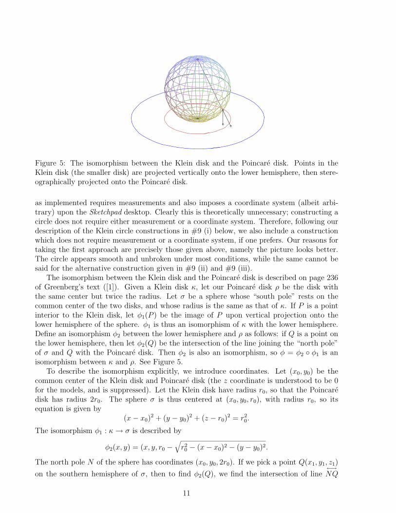
Figure 5: The isomorphism between the Klein disk and the Poincare disk. Points in theKlein disk (the smaller disk) are projected vertically onto the lower hemisphere, then stere-ographically projected onto the Poincare disk.

as implemented requires measurements and also imposes a coordinate system (albeit arbi-trary) upon the Sketchpad desktop. Clearly this is theoretically unnecessary; constructing acircle does not require either measurement or a coordinate system. Therefore, following ourdescription of the Klein circle constructions in #9 (i) below, we also include a constructionwhich does not require measurement or a coordinate system, if one prefers. Our reasons fortaking the first approach are precisely those given above, namely the picture looks better.The circle appears smooth and unbroken under most conditions, while the same cannot besaid for the alternative construction given in #9 (ii) and #9 (iii).

The isomorphism between the Klein disk and the Poincare disk is described on page 236of Greenberg’s text ([1]). Given a Klein disk κ, let our Poincare disk ρ be the disk withthe same center but twice the radius. Let σ be a sphere whose “south pole” rests on thecommon center of the two disks, and whose radius is the same as that of κ. If P is a pointinterior to the Klein disk, let φ1(P ) be the image of P upon vertical projection onto thelower hemisphere of the sphere. φ1 is thus an isomorphism of κ with the lower hemisphere.Define an isomorphism φ2 between the lower hemisphere and ρ as follows: if Q is a point onthe lower hemisphere, then let φ2(Q) be the intersection of the line joining the “north pole”of σ and Q with the Poincare disk. Then φ2 is also an isomorphism, so φ = φ2 ◦ φ1 is anisomorphism between κ and ρ. See Figure 5.

To describe the isomorphism explicitly, we introduce coordinates. Let (x0, y0) be thecommon center of the Klein disk and Poincare disk (the z coordinate is understood to be 0for the models, and is suppressed). Let the Klein disk have radius r0, so that the Poincaredisk has radius 2r0. The sphere σ is thus centered at (x0, y0, r0), with radius r0, so itsequation is given by

(x− x0)2 + (y − y0)

2 + (z − r0)2 = r2

0.

The isomorphism φ1 : κ → σ is described by

φ2(x, y) = (x, y, r0 −√

r20 − (x− x0)2 − (y − y0)2.

The north pole N of the sphere has coordinates (x0, y0, 2r0). If we pick a point Q(x1, y1, z1)

on the southern hemisphere of σ, then to find φ2(Q), we find the intersection of line←→NQ

11

with the plane z = 0. This line is represented by the parametric equations

x = (x1 − x0)t + x0

y = (y1 − y0)t + y0

z = (z1 − 2r0)t + 2r0.

Setting z = 0 yields t = −2r0

z1−2r0. Substituting for x and y in the parametric equations yields

φ2(x1, y1, z1) =

(−2r0(x1 − x0)

z1 − 2r0

+ x0,−2r0(y1 − y0)

z1 − 2r0

+ y0

).

Thus, the composition of φ = φ2 ◦ φ1 gives us our isomorphism between κ and ρ, definedby

(x, y) 7→(−2r0(x− x0)

z1 − 2r0+ x0,

−2r0(y − y0)z1 − 2r0

+ y0

), where z1 = r0 −

√r20 − (x− x0)2 − (y − y0)2.

The Geometer’s Sketchpad script kd_to_pd.gss implements this isomorphism. Givena point (x, y) in the Klein disk, the script returns the corresponding point φ(x, y) in thePoincare disk.

The inverse isomorphism φ−1 : ρ → k is found in a similar manner; the order of operationsis simply reversed. Given a point P ′ in the Poincare disk, we find the intersection of the linejoining P ′ to the north pole of σ with the lower hemisphere of σ. We then project that pointvertically downward to find the corresponding point P = φ−1(P ′) in the Klein disk.

If P ′ has coordinates (x′, y′), then the line←→NP ′ can be expressed parametrically by the

system:

x = (x′ − x0)t + x′

y = (y′ − y0)t + y′

z = −2r0t.

This line intersects the lower half-sphere when

t =−(y′ − y0)

2 − (x′ − x0)2

(y′ − y0)2 + (x′ − x0)2 + 4r20

=−d2

d2 + 4r20

,

where d =√

(y′ − y0)2 + (x′ − x0)2 is the distance from P ′ to the center of the Poincaredisk. Substituting into our parametric equations, we find the intersection point on the lowerhemisphere is

x =−d2(x′ − x0)

d2 + 4r20

+ x′

y =−d2(y′ − y0)

d2 + 4r20

+ y′

z =2r0d

2

d2 + 4r2.

12

c

Poincare Disk

Klein Disk

X

X'

O'

P'

OP

1

c2

Figure 6: Constructing the Klein circle centered at O and with radius OP , using the iso-morphism φ between the Klein disk and the Poincare disk.

Then our inverse image P = φ−1(P ′) in the Klein disk is the point (x, y), where x and yhave the values just defined. That is,

φ−1(x′, y′) =

(−d2(x′ − x0)

d2 + 4r20

+ x′,−d2(y′ − y0)

d2 + 4r20

+ y′)

.

The Geometer’s Sketchpad script pd_to_kd.gss implements the inverse isomorphism.Given a point (x′, y′) in the Poincare disk, the script returns the corresponding pointφ−1(x′, y′) in the Klein disk.

Finally, we are ready to describe how we construct Klein circles.

9. i) (kcntrpt.gss) Construct a Klein circle, given its center and a point on the circle.

Given: Klein points O and P .

To Construct: The K-circle centered at O with radius OP .

a) Using the isomorphism φ between the Klein disk and Poincare disk describedabove (implemented with the tool kd_to_pd.gss), find the images O′ = φ(O)and P ′ = φ(P ) of O and P , respectively in the Poincare disk.

b) Using a Poincare disk model tool (such as Bennett’s centrpt.gss), constructthe Poincare circle centered at O′ with radius O′P ′. Call this circle c1.

c) Choose a point X ′ on the circle c1 defined in the previous step. Using theinverse isomorphism φ−1 between the Poincare disk and the Klein disk (im-plemented with the tool pd_to_kd.gss), find the inverse image X = φ−1(X ′)in the Klein disk.

The Klein circle c2 centered at O with radius OP is the locus of points X as thedriver point X ′ moves around circle c1. See Figure 6.

ii) (kreflpt.gss) Construct the reflection of a point about a Klein line.

Given: Klein points A and M .

13

m

t

A'

T

T'P

S

S'

Q

M

A

Figure 7: Constructing the reflection of a point about a line in the Klein model.

To Construct: The point A′ (distinct from A) on K-line←→AM such that AM ∼= A′M

in the Klein sense. A′ is thus the image of A under reflection about the K-line

through M which is perpendicular (in the Klein sense) to←→AM .

(Greenberg outlines this construction on p. 262 of [1].)

a) Construct the K-line passing through A and M . Call this line t.

b) Construct the pole Q of t using Construction #5 (i) given above.

c) Draw Euclidean line←→QA. This line intersects γ at two points, S and S ′.

d) Draw Euclidean line←→QM . The portion of this line which is a chord of γ is a

K-line through M which is perpendicular to t. Call this line m.

e) Construct the pole P of m using Construction #5 (i) given above.

f) Draw the Euclidean lines←→PS and

←→PS ′. Each of these lines intersects γ at

another point on γ. Call these additional ideal points T and T ′, respectively.

g) Draw Euclidean chord TT ′. TT ′ intersects K-line t at a point A′.

A′ is the desired reflection of A about line m, with AM ∼= A′M in the Klein sense.See Figure 7.

iii) Here we provide an alternate construction for a Klein circle given its center anda point on the circle. This construction does not require measurement or a coor-dinate system, but the resulting circle tends not to be as cleanly represented inGeometer’s Sketchpad as that of Construction #9 (i) above.

Given: Klein points O and P .

To Construct: The K-circle centered at O with radius OP .

a) Construct the Euclidean circle c1 centered at O with Euclidean radius OP .

b) Choose a point Q on circle c1.

c) Draw line←→OQ.

14

c1

P'

M

Q

O

P

c 2

Figure 8: Constructing the Klein circle centered at O and with radius OP (without usingmeasurement).

l

P

T

M

B

A

O

1c

Figure 9: Constructing the Klein circle centered at O and with radius OP congruent to AB.

d) Construct the reflection of point P about ray−→OQ. To do this, drop a K-

perpendicular from P to line←→OQ and let M be the point of intersection.

Reflect point P using Construction #9 (i) above. Let P ′ be the image of thisreflection.

e) By construction, OP ∼= OP ′ in the sense of Klein.

The Klein circle c2 centered at O with radius OP is the locus of points P ′ as Qtravels around the Euclidean circle c1. Note that c2 is not a Euclidean circle. SeeFigure 8.

10. i) (kcntrrd.gss) Construct a Klein circle, given its center and two points, the seg-ment between which determines the radius of the circle.

Given: Klein points O, A, and B.

15

To Construct: The K-circle centered at O and consisting of all points P such thatOP ∼= AB in the Klein sense.

a) Using the isomorphism φ between the Klein disk and Poincare disk describedabove (implemented with the tool kd_to_pd.gss), find the images O′ =φ(O), A′ = φ(A) B′ = φ(B) of O, A, and B, respectively in the Poincaredisk.

b) Using a Poincare disk model tool (such as Bennett’s centrrad.gss), constructthe Poincare circle centered at O′ and consisting of all points P ′ such thatO′P ′ ∼= A′B′ in the Poincare disk sense. Call this circle c1.

c) Choose a point X ′ on the circle c1 defined in the previous step. Using theinverse isomorphism φ−1 between the Poincare disk and the Klein disk (im-plemented with the tool pd_to_kd.gss), find the inverse image X = φ−1(X ′)in the Klein disk.

The Klein circle c2 centered at O with radius OP ∼= AB is the locus of points Xas the driver point X ′ moves around circle c1.

ii) The construction in #10(i) above is implemented using coordinates and mea-surement, since it involves the isomorphism φ between the Poincare disk and theKlein disk. An alternate construction is provided here which does not requireintroducing coordinates or measurements, but the resulting circle tends not to beas cleanly represented in Geometer’s Sketchpad as that of #10(i).

Given: Klein points O, A, and B.

To Construct: The K-circle centered at O with radius OP , where OP ∼= AB inthe Klein sense.

a) Draw segment OA. Let K-line ` be the perpendicular bisector of segmentOA, using Construction #8 (ii) above.

b) Drop a K-perpendicular from point B to line ` at a point M , using Construc-tion #7 above.

c) Reflect point B about line ` using Construction #9 (ii) above. Let P bethe image of this reflection. If we let T be the point of intersection of OAand `, then we can see that OP ∼= AB in the sense of Klein by using twosets of congruent triangles: ∆TPM ∼= ∆TBM by SAS. This in turn gives us∆TPO ∼= ∆TBA by SAS, and our result follows.

d) Construct the K-circle c1 centered at O with radius OP , using Construction#9 (iii) above.

Circle c1 is our desired circle. See Figure 9.

We finish our discussion of the Klein circle tools and the Klein disk in general with adescription of the three scripts kintcirc.gss, kintlncr.gss, and kintsgcr.gss. These toolsare designed to respectively find the intersection point(s) of two Klein circles, to find theintersection point(s) of a Klein circle with a Klein line, and to find the intersection point(s)of a Klein circle with a Klein line segment. As discussed above, these tools are necessarybecause of the limitations of the Geometer’s Sketchpad software; Klein circles are represented

16

as loci of points, and current versions of Sketchpad are not capable of finding intersectionsof objects which are loci.

As with the circle constructions, the construction of these “intersection” scripts use theisomorphism φ between the Klein disk and Poincare disk. The idea of the intersection scriptsis as follows: given two objects in the Klein disk which we wish to intersect, we find theirimages under the isomorphism φ in the Poincare disk. We find the intersection of thesecorresponding images in the Poincare disk using the usual Sketchpad tools. We find theinverse images of these intersection points to find the desired intersections in the Klein disk.

4 Poincare Half-Plane Model Scripts

In the Poincare Half-plane model of hyperbolic geometry, we fix a (Euclidean) line andarbitrarily choose one side of that line to be the “upper half-plane.” For intuitive purposes,we generally use the x-axis as our line and let the set of points whose y-coordinate is positivebe the upper half-plane. “Points” in this model are interpreted to be points in the upperhalf-plane (not including the x-axis), and “lines” are interpreted to be either vertical rayswith endpoint on the x-axis, or, more generally half circles whose center lies on the x-axis.(The constructions below work in the more general case, not for the special case of the lineswhich are rays.)

Below are descriptions of basic constructions 1–10 in the Poincare half-plane model. Thedescriptions supplement the associated Geometer’s Sketchpad scripts for the constructions.Although I give descriptions for all ten constructions, others have produced scripts for theseconstructions previously. As noted earlier, Bennett has created scripts for items 1–4 in thehalf-plane model. His scripts may be found at

http://www.keypress.com/sketchpad/misc/sibley/sibley.htm.

These scripts are titled hyp line.gss, hyp seg.gss, hyp dist.gss, and hyp angl.gss, andconstruct hyperbolic lines and segments, and measure hyperbolic distances and angles, re-spectively, in the Poincare half-plane model. My description of “Construction” #3 is slightlydifferent from Bennett’s. I choose a slightly different unit for measuring length, for ease ofuse of hyperbolic trigonometry. As such, I give a description of my construction/calculationscript (phlength.gss), rather than his. The remaining scripts given here have been writtenby this author.

Peil has also written several scripts for the half-plane model, which may be found at

http://classweb.mnstate.edu/peil/Projects/geo.html.

Although several of the constructions described here appear to duplicate Peil’s work, itshould be noted that several constructions differ in their fundamentals (Peil uses coordinategeometry for some of his constructions).

As in the Beltrami-Klein case, each construction corresponds to an available Geometer’sSketchpad script. The name of the associated script is given in bold-face next to the num-ber of the construction. In Sketchpad, the script tools assume that one is performing theconstructions using a fixed line defined by two points labelled “A” and “B”. Although onecan typically use any line so defined, it is helpful to use the x-axis as the defining line. In

17

c1

O

A

B

Figure 10: Constructing the line through A and B in the Poincare Half-plane model.

particular, Sketchpad can become confused as to which side of line←→AB is the “upper half-

plane,” an ambiguity which is less troublesome when←→AB is the x-axis. The Sketchpad file

“poinhalf.gsp” contains a startup figure in which A and B are points on the x-axis. Thesimplest way to use the script tools is to create a directory, perhaps called “poinhalf,” inwhich all the scripts and “poinhalf.gsp” is stored. Set the script tool directory in Sketchpadto be “poinhalf,” and the tools will be accessible from the Sketchpad desktop.

As noted in the introduction, in addition to the standard ten constructions, we includeconstructions which find the midpoint of a half-plane segment (see item #8(i) below) and thereflection of a point about a half-plane line (see item #9(i)). In all the constructions we willuse terms such as “PH-line” and “PH-circle” as shorthand for “Poincare half-plane line” and“Poincare half-plane circle”. This will distinguish between the non-Euclidean constructionsand their Euclidean counterparts.

1. (Bennett’s hyp line.gss) Construct a PH-line, given two points on the line.

Given: Two points A and B in the PH-plane.

To Construct: PH-line←→AB, i.e. the half-circle centered on the x-axis and passing

through A and B.

a) Construct Euclidean segment AB.

b) Let ` be the Euclidean perpendicular bisector of AB. Assuming that A and B donot lie on the same vertical line, let O be the intersection of ` and the x-axis.

c) Let c1 be the circle centered at O with radius OA.

The half of circle c1 which lies in the upper half plane is the PH-line through A andB. See Figure 10.

2. (Bennett’s hyp seg.gss) Construct a PH-line segment, given the endpoints of thesegment.

Given: Two points A and B in the PH-plane.

18

P Q

B

A

Figure 11: Calculating the length of a line segment AB in the Poincare Half-plane model.

To Construct: PH-segment←→AB, i.e. the arc of the circle centered on the x-axis,

contained entirely in the upper half-plane, and with endpoints A and B.

a) Construct the PH-line←→AB as described in Construction #1 above.

b) Let PH-segment AB be the arc of the←→AB which is contained entirely in the upper

half-plane, and has endpoints A and B.

3. (phlength.gss) Measure the length of a PH-line segment.

Given: Two points A and B in the Poincare half-plane.

To Measure: The PH-length of segment AB.

a) Construct the PH-line←→AB. Let P and Q be the ideal points of this PH-line, i.e.

the points of intersection of the x-axis and the circle centered on the x-axis whichpasses through A and B.

b) Find each of the following Euclidean lengths: AP , AQ, BP , BQ.

c) Define the cross-ratio (AB, PQ) by

(AB, PQ) =AP/AQ

BP/BQ.

Let d = |`n(AB,PQ)|. Then d is the PH-length of segment AB. d is independentof the labelling of P and Q (i.e. their labelling could be reversed without affectingd). See Figure 11.

Note: As in the length definition for the Klein model, other definitions (using adifferent log base or scaling factor) are possible, but this one allows for easy use ofhyperbolic trig formulas.

4. (Bennett’s hyp angl.gss) Calculate the measure of an angle.

Given: Points A, B, and C in the Poincare half-plane.

To Calculate: the PH-measure of 6 ACB.

19

m n

TS

PO

B

C

A

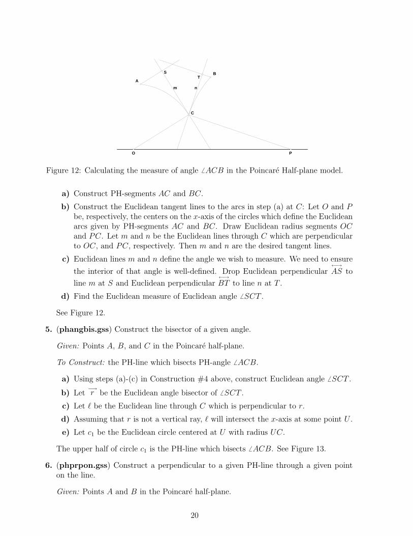
Figure 12: Calculating the measure of angle 6 ACB in the Poincare Half-plane model.

a) Construct PH-segments AC and BC.

b) Construct the Euclidean tangent lines to the arcs in step (a) at C: Let O and Pbe, respectively, the centers on the x-axis of the circles which define the Euclideanarcs given by PH-segments AC and BC. Draw Euclidean radius segments OCand PC. Let m and n be the Euclidean lines through C which are perpendicularto OC, and PC, respectively. Then m and n are the desired tangent lines.

c) Euclidean lines m and n define the angle we wish to measure. We need to ensure

the interior of that angle is well-defined. Drop Euclidean perpendicular←→AS to

line m at S and Euclidean perpendicular←→BT to line n at T .

d) Find the Euclidean measure of Euclidean angle 6 SCT .

See Figure 12.

5. (phangbis.gss) Construct the bisector of a given angle.

Given: Points A, B, and C in the Poincare half-plane.

To Construct: the PH-line which bisects PH-angle 6 ACB.

a) Using steps (a)-(c) in Construction #4 above, construct Euclidean angle 6 SCT .

b) Let−→r be the Euclidean angle bisector of 6 SCT .

c) Let ` be the Euclidean line through C which is perpendicular to r.

d) Assuming that r is not a vertical ray, ` will intersect the x-axis at some point U .

e) Let c1 be the Euclidean circle centered at U with radius UC.

The upper half of circle c1 is the PH-line which bisects 6 ACB. See Figure 13.

6. (phprpon.gss) Construct a perpendicular to a given PH-line through a given pointon the line.

Given: Points A and B in the Poincare half-plane.

20

c1

l

r

U

T

S

B

C

A

Figure 13: Constructing the angle bisector of an angle in the Poincare Half-plane model.

To Construct: the PH-line (i.e. Euclidean half-circle) through A which is perpendicular(in the PH-sense) to the PH-line joining A and B.

a) Construct the PH-line←→AB as described in Construction #1 above. As a Euclidean

half-circle, let this PH-line have center O (on the x-axis).

b) Construct Euclidean segment OA.

c) Construct the Euclidean line ` through A which is perpendicular to segment OA.

Line ` is thus the tangent to the PH-line←→AB at point A.

d) Assuming OA is not a vertical line segment, ` intersects the x-axis at some pointP .

e) Construct the Euclidean half-circle m centered at P and passing through pointA.

PH-line m is the desired line. Note that by construction, Euclidean line←→PA is perpen-

dicular to segment OA. On the other hand, Euclidean lines←→PA and OA are tangent

to the PH-lines←→AB and m, respectively. By the definition of perpendicularity in the

half-plane model, then, m ⊥←→AB. See Figure 14.

7. (phprpoff.gss) Construct a perpendicular to a given PH-line through a given pointnot on the line.

Given: Points A and B defining PH-line←→AB and point C not on

←→AB.

To Construct: PH-line (i.e. Euclidean half-circle) ` through C which is perpendicular(in the PH-sense) to the PH-line joining A and B.

a) Construct the PH-line←→AB as described in Construction #1 above. As a Euclidean

half-circle, let this PH-line have center O. Extend the half-circle to a full-circlec1.

b) Construct Euclidean line←→OC. Let D be the point above the x-axis where the

PH-line←→AB meets Euclidean line

←→OC.

21

m

l

PO

A

B

Figure 14: Constructing the PH-line through A which is perpendicular to←→AB in the Poincare

Half-plane model.

c1

c2

G

D

F

E

O

A

B

C

Figure 15: Constructing the PH-line through C which is perpendicular to←→AB in the Poincare

Half-plane model.

c) Construct the Euclidean circle c2 centered at O and passing through point C.

d) Construct the Euclidean line through O which is perpendicular to Euclidean line←→OC. Let this line intersect circle c1 at point E and circle c2 at point F , where Eand F lie above the x-axis.

e) Construct Euclidean line←→DF .

f) Construct the line through E which is parallel to←→DF . Let this line intersect

Euclidean line←→OC at point G.

g) Construct the PH-line←→CG as described in Construction #1 above.

PH-line←→CG is the desired line. The Euclidean half-circles

←→CG and

←→AB intersect or-

thogonally, so the lines are perpendicular in the Poincare half-plane sense. See Figure15.

8. i) (phmidpt.gss) Construct the midpoint of a PH-line segment.

Given: Points C and D.

22

c2c1L

K

J

I/M

HF G

D

C

Figure 16: Constructing the midpoint of PH-line segment AB in the Poincare Half-planemodel.

To Construct: the point M lying on PH-segment CD which is the midpoint (inthe PH-sense) of CD.

a) Construct PH-segment (i.e. Euclidean circle arc) CD. Extend this arc to aEuclidean circle c1, centered at the point F .

b) Construct Euclidean line←→CD. Assuming

←→CD is not parallel to the x-axis, let

G be the point of intersection of←→CD and the x-axis.

c) Let H be the Euclidean midpoint of Euclidean segment FG which is part ofthe x-axis.

d) Let c2 be the Euclidean circle centered at H and passing through G.

e) Circles c1 and c2 intersect in two points on opposite sides of the x-axis. Theintersection point M which is above the x-axis is the midpoint of PH-segmentCD.

This completes the essence of the construction; however, Geometer’s Sketchpadhas some difficulty in deciding which intersection point in step (e) “is above the x-axis.” The remaining construction steps select the correct point without resortingto coordinate geometry:

f) Call the intersection points from step (e) points I and J . Construct Euclideanline segment IJ .

g)←→IJ is perpendicular to the x-axis at some point K. In addition,

←→IJ intersects

Euclidean segment CD at some point L.

h) Construct Euclidean ray−→KL. By construction, this ray emanates from a

point on the x-axis and “points in the positive y-direction.”

i) Let M be the intersection of ray−→KL with circle c2.

By construction, M will be either point I or point J , whichever has positivey-coordinate. See Figure 16.

ii) (phprpbis.gss) Construct the perpendicular bisector of a PH-line segment.

Given: Points C and D.

23

To Construct: the perpendicular bisector (in the PH-sense) of the PH-segmentCD.

a) Construct the midpoint M of PH-segment CD as in Construction #8 (i) above.

b) Construct the PH-line ` through M which is perpendicular to PH-segment CD(see Construction # 6 above).

9. i) (phreflpt.gss) Construct the reflection of a point about a PH-line.

Given: Points A and M in the Poincare half-plane.

To Construct: The point A′ on PH-line←→AM such that AM ∼= A′M in the Poincare

sense. A′ is thus the image of A under reflection about the PH-line through M

which is perpendicular to←→AM .

a) Construct the PH-line←→AM . Let c1 be the Euclidean half-circle which is this

PH-line.

b) Using Construction #6 above, construct the PH-line m through M which is

perpendicular to PH-line←→AM . As a Euclidean half-circle, let this PH-line

have center O.

c) Draw Euclidean line←→OA.

←→OA intersects the half-circle c1 at two points, A

and another point A′.

A′ is the desired reflection of A about line m with AM ∼= A′M . See Figure 17.

This completes the essence of the construction; however, Geometer’s Sketchpad

has some difficulty in deciding which point of intersection of line←→OA with circle

c1 is A and which is the desired reflection A′. To resolve this difficulty, I includethe following additional constructions:

d) After constructing line←→OA, let C and D be the points of intersection of this

line with circle c1. (One of C and D is point A, and one is A′.)e) Construct Euclidean segment CD and find its Euclidean midpoint E.

f) Draw ray−→AE. This ray will intersect circle c1 at either C or D. This point

of intersection is our desired reflection A′.

ii) (phcntrpt.gss) Construct a PH-circle, given its center and a point on the circle.

Given: Points O and P in the Poincare half-plane.

To Construct: the PH-circle centered at O with PH-radius OP .

Note: A PH-circle is also a Euclidean circle, albeit with a different “center.” TheEuclidean center of our desired circle will lie on the same vertical line as O.

a) Construct the Euclidean line ` through O which is perpendicular to the x-axis.

b) Using Construction # 9(i) above, let P ′ be the image of P under PH-reflection

about the line through O perpendicular to PH-line←→OP . Thus OP ∼= OP ′ in

the PH-sense and P ′ is a second point on the desired circle.

24

m

c1

A'

O

M

A

Figure 17: Constructing the reflection A′ of a point A about a line in the Poincare Half-planemodel.

c1

m

l

O'

P'

O

P

Figure 18: Constructing PH-circle centered at O with PH-radius OP in the Poincare Half-plane model.

c) Draw Euclidean segment PP ′ and construct its Euclidean perpendicular bi-sector m.

d) Assuming m is not a vertical line, let O′ be the intersection of lines m and `.

e) Let c1 be the Euclidean circle centered at O′ and passing through P (and P ′

as well).

Circle c1 is our desired circle. See Figure 18.

10. (phcntrrd.gss) Construct a PH-circle, given its center and two points, the distancebetween which determines the radius of the circle.

Given: Points O, A, and B in the Poincare half-plane.

To Construct: The PH-circle centered at O with radius OP , where OP ∼= AB in thePH-sense.

a) Draw PH-segment OA. Let PH-line ` be the perpendicular bisector of segmentOA, using Construction #8 (ii) above.

25

c1

m

l

P

M

O

B A

Figure 19: Constructing PH-circle centered at O with PH-radius OP congruent to AB inthe Poincare Half-plane model.

b) Drop a PH-perpendicular from point B to line ` at a point M , using Construction#7 above. Call this line m.

c) Reflect point B about line ` using Construction #9 (i) above. Let P be the imageof this reflection, noting that P lies on PH-line m.

d) Construct the PH-circle c1 centered at O with radius OP , using Construction #9(ii) above.

Circle c1 has center O and radius OP . By construction, OP ∼= AB. See Figure 19.

References

[1] M. Greenberg. Euclidean and Non-Euclidean Geometries: Development and History. W.H. Freeman and Company, New York, 3rd edition, 1993.

[2] D. Hilbert. Foundations of Geometry. Open Court Publishing Company, Peru, IL, 1994.

[3] W. Prenowitz and M. Jordan. Basic Concepts of Geometry. Ardsley House Publishers,New York, 1965.

[4] S. Stahl. The Poincare Half-Plane: A Gateway to Modern Geometry. Jones and BartlettPublishers, Boston, 1993.

26