hyperspectral imaging spectroscopy: a promising method for ... · butz et al.: hyperspectral...

Hyperspectral imaging spectroscopy:a promising method for thebiogeochemical analysis of lakesediments

Christoph ButzMartin GrosjeanDaniela FischerStefan WunderleWojciech TylmannBert Rein

source: https://doi.org/10.7892/boris.70461 | downloaded: 7.6.2020

Hyperspectral imaging spectroscopy: a promisingmethod for the biogeochemical analysis of lake sediments

Christoph Butz,a,* Martin Grosjean,a Daniela Fischer,a Stefan Wunderle,a

Wojciech Tylmann,b and Bert Reinc

aUniversity of Bern, Institute of Geography and Oeschger Centre for Climate Change Research,Erlachstrasse 9a, Bern CH-3012, Switzerland

bUniversity of Gdansk, Institute of Geography, Bazynskiego 4, Gdansk 80-952, PolandcGeoConsult Rein, Gartenstrasse 26-28, Oppenheim D-55276, Germany

Abstract. We investigate the potential of hyperspectral imaging spectrometry for the analysis offresh sediment cores. A sediment-core-scanning system equipped with a camera working in thevisual to near-infrared range (400 to 1000 nm) is described and a general methodology forprocessing and calibrating spectral data from sediments is proposed. We present an applicationfrom organic sediments of Lake Jaczno, a freshwater lake with biochemical varves in northernPoland. The sedimentary pigment bacteriopheophytin a (BPhe a) is diagnostic for anoxia inlakes and, therefore, an important ecological indicator. Calibration of the spectral data (BPhea absorption ∼800 to 900 nm) to absolute BPhe a concentrations, as measured by high-perfor-mance-liquid-chromatography, reveals that sedimentary BPhe a concentrations can be estimatedfrom spectral data with a model uncertainty of ∼10%. Based on this calibration model, we usethe hyperspectral data from the sediment core to produce high-resolution intensity maps and timeseries of relative BPhe a concentrations (∼10 to 20 data points per year, pixel resolution70 × 70 μm2). We conclude that hyperspectral imaging is a very cost- and time-efficient methodfor the analysis of lake sediments and provides insight into the spatiotemporal structures of bio-geochemical species at a degree of detail that is not possible with wet chemical analyses. © 2015Society of Photo-Optical Instrumentation Engineers (SPIE) [DOI: 10.1117/1.JRS.9.096031]

Keywords: hyperspectral imaging; image acquisition/recording; reflectance; nondestructivetesting; sedimentary pigments; bacteriopheophytin.

Paper 15147 received Feb. 25, 2015; accepted for publication Jun. 4, 2015; published online Jul.7, 2015.

1 Introduction

In situ imaging spectroscopy has great potential for fast, nondestructive, inexpensive, and high-resolution analysis of material compositions, supplementing established physical or chemicalanalytical methods. The identification of materials and substances according to their diagnosticspectral properties in the visible and infrared range has been extensively used at both remote andin situ scales.1–4 Typically, spectroscopic data from laboratory- or hand-held scanners are usedfor ground measurements to validate aerial or satellite remote sensing data or, for example, inthe mining industry for geologic core logging.5–8 However, in contrast to airborne or satelliteplatforms, in situ scanners still mostly use point measurements instead of imaging methods,which limits the information about spatial variability in a given sample.

Recent advances in imaging spectrometry have opened a new field of scanning techniques forin situ or laboratory scales with hyperspectral resolution: hundreds of contiguous spectral bandsat high spatial resolution (micrometer to nanometer scales) can be measured.9–12 This offers greatopportunities in environmental research.

In environmental and earth-science research, biological, geochemical and physical propertiesof lake and marine sediments are widely used as records of past and recent environmental

*Address all correspondence to: Christoph Butz, E-mail: [email protected]

1931-3195/2015/$25.00 © 2015 SPIE

Journal of Applied Remote Sensing 096031-1 Vol. 9, 2015

http://dx.doi.org/10.1117/1.JRS.9.096031





mailto:[email protected]




changes.13 However, sample preparation and measurement with physical and chemical methodsis generally very time consuming and expensive, which often limits the number of samples thatcan be analyzed. Therefore, nondestructive scanning and imaging methods have become increas-ingly important.14 In contrast to other well-established scanning methods like micro-x-ray-fluo-rescence (μXRF) or computer tomography, spectrometric methods are able to detect, based ontheir unique spectral fingerprints, chemical compounds and substances rather than chemicalelements or physical properties (e.g., sediment density).

Spectroscopic methods using reflectance in the “visual to near-infrared range” (VNIR) havebeen used for decades for color logging (Munsell, CIELAB or other XYZ-based color spaces) ongeologic sediment samples.15–17 The first applications for specific material identification andinterpretation for different species were developed by Refs. 18–22. References 23–25, for exam-ple, measured spectral data directly from fresh marine or lake sediment cores using point meas-urement photospectrometers (GretagMcBeth Spectrolino or ASD FieldSpec Pro). They derivedspectral indices from reflectance spectra, which they could quantitatively calibrate to concen-trations of chlorophyll a (Chl a), chlorins, lutein, and organic carbon. Furthermore, relative claycontents (illite, chlorite, and glauconite) could be estimated. All of these substances providevaluable information about environmental changes.

Following this approach, several authors successfully applied this method on recent fresh-water lake sediments and demonstrated that, in specific cases, spectral data from point-measure-ments (2-mm sensor fields) along a sediment core could be directly calibrated to meteorologicaltime series. In these cases, spectral data could be used as high-resolution proxies for quantitativeclimate reconstructions.26–32 In this study, we use a VNIR imaging spectrometer designed for useas a sediment core-scanning system and present a case study for spectral analysis of fresh lakesediments. First, we describe the technical equipment and the general methodology (workflow)that was used to acquire and process the spectral data. For illustration, the second part of thisarticle presents a case study on organic sediments from a freshwater lake in Poland. We discussthe sample preparation for scanning and present a calibration procedure to calibrate spectral datato concentrations of specific substances, which were retrieved by established chemical analyticalmethods (e.g., high-performance-liquid-chromatography, HPLC). In our example, we show thatconcentrations of sedimentary bacteriopheophytin a (BPhe a) can be inferred at very high spatialresolution (70 × 70 μm2) for spatial maps and time series of BPhe a concentrations in a sedimentcore. BPhe a is mainly produced by bacteria under anoxic conditions and is thus most appro-priate for the documentation of environmental change in freshwater environments.

2 Hyperspectral Imaging of Lake Sediments

2.1 General Methodology (Workflow)

The general methodology for spectral analysis of lake sediments consists of four steps (seeFig. 1; for more details, refer to Secs. 2.3–2.5 and 3 case study):

(1) Data acquisition [Sec. 2.3, Fig. 1(a)]: the camera settings are optimized (field of view(FOV), focus, frame rate, exposure time, and moving speed of sample tray). The sedi-ment core (sample) surface is cleaned and prepared. A scan of the white and darkstandards and the sample is performed.

(2) Data preprocessing [Sec. 2.4, Fig. 1(b)]: spectral data of the sediment core are calibratedto a white and dark standard. Regions of interest (ROIs) are defined and extracted fromthe calibrated image file of the core. A set of images [RGB, near infrared (NIR), colorinfrared (CIR) band combinations] is made for visual inspection of the data. Dependingon the type of sample and quality of the scan, additional denoising can be performed onthe dataset.

(3) Data postprocessing [Sec. 2.5, Fig. 1(c)]: here, we use the Spectral Hourglass Wizard ofthe ENVI software for the extraction of the purest spectra in the sample (endmembers).After determination of the endmembers, spectral features within the endmembers arecompared to diagnostic spectral indices known from the literature. These indices maythen be modified and calculated for all spectra of the sample scanned. Unknown spectral

Butz et al.: Hyperspectral imaging spectroscopy: a promising method for the biogeochemical. . .


Fig. 1 General methodology for the hyperspectral analysis of lake sediments with the SCS. Fordetails see Secs. 2 and 3. (a) Data acquisition, (b) preprocessing, (c) postprocessing, and(d) output.



features may be marked and calculated for further investigation. Spectral endmemberscan be compared to spectral libraries and used as classes for whole-sample classification.

(4) Output [Sec. 3, Fig. 1(d)]: typical types of data output include gray scaled and colormapped single-band images of spectral indices for visual inspection and as arrays,time series of spectral information along selected transects of the sediment core andstatistics. Endmembers are stored as spectral libraries and graphs along with additionalmetadata and processing steps. Additional data analyses and outputs are made using Rstatistics.

2.2 Technical Instrument Description

Hyperspectral analyses are conducted using a sediment-core-scanning system (SCS, developedby Specim Ltd.) in combination with a Specim PFD-xx-V10E camera and a SchneiderKreuznach Xenoplan 1.9/35 lens. The SCS [Fig. 2(a)] consists of the spectral camera mountedabove an illumination unit, a movable sample tray and a control unit connected to a personalcomputer. Images are measured in the VNIR spectrum from 400 to 1000 nm. The slit is 30 μmwide and the spectral resolution is 2.8 nm sampled at an interval of 0.78 nm or binned into 1.6,3.2 or 6.4-nm intervals [Figs. 2(b) and 2(c)].33 Due to a small horizontal angle of view of theobjective lens (∼15.7 deg), errors related to lens aberration are insignificant. This permits theanalysis of samples between ∼45 and 120 mm widths and an on-sample spatial pixel resolutionbetween 40 and 90 μm. Illumination is provided by a dome-like unit equipped with two arrays of13 halogen lamps each, aligned across-track to evenly illuminate the sample. Illumination isindirect. The light is projected on a concave diffusor plate and directed in such a way that it hitsthe sample at multiple angles.

The system uses a push broom technique. During a measurement, the tray with the sedimentsample moves underneath the camera and illumination unit. The camera measures the lightreflected from the sample line-by-line through a slit in the illumination unit. A PC interface(ChemaDAQ software, Specim Ltd.) controls the scanning system. Raw data are stored digitallyon the hard drive. The raw data are compatible with ENVI’s binary format with separate header

Fig. 2 (a) Overview of the Specim hyperspectral sediment-core scanner. (b) Principle of thehyperspectral line scan camera. (c) Camera specifications. (d) Image of the focus table.



file. The dark reference (closed shutter) and the white reference [BaSO4 ceramic plate, Fig. 2(d)]are taken automatically in the beginning of each scan and are stored in separate files.

2.3 Data Acquisition

2.3.1 Sediment sample preparation

Sediment cores are typically retrieved in core liners of 1 to 1.5 m in length and 6 to 9 cm indiameter. In the lab, the cores are split lengthwise into two half cores and sometimes also sub-sampled with U-channels. Our system allows for sediment cores up to 12 × 145 cm2. In additionto fresh sediment cores, flat surfaces of epoxy-resin embedded and polished sediment slabs maybe scanned.

After opening, the fresh sediment surface is cleaned with a sharp metal blade or a knife. Thesediment surface is prepared in a way that means it is as flat as possible (allows for better focus)and the finest sediment structures are visible.

Specular reflection may be a problem for samples with high water content, especially withexcess water on the surface. To minimize such effects of water reflection, wet sediments shouldbe left to dry until surface water is sufficiently reduced. This process may take up to 24 h. This isparticularly important for very dark sediments with generally low reflection.

2.3.2 Scanner and camera adjustments

Optimal settings for scanning depend on the sample type and its dimensions, as well as severalhardware adjustments (e.g., camera focus), parameters and choices to be made by the operator.Three steps are needed to focus the camera. First, a vertically moveable table [focus table,Fig. 2(d)] at the front of the sample tray is adjusted to the same height as the sample surface.The illumination unit is then positioned just above the focus table and the sample surface.Second, the FOV is set by changing the vertical position of the camera above the focustable. Third, tuning of the camera focus is done by manual adjustment of the lens. The focustable contains a grid of an alternating black and white pattern, which is used in combinationwith the computer monitor to focus the image. The focus table, therefore, corresponds tothe focal plane of the later image.

Software-based settings (ChemaDAQ) include binning, frame rate, movement speed of thesample tray, exposure time, and scanning range. Spectral binning controls the spectral samplingrate. Typically, scanning is performed at the highest spectral sampling resolution (∼0.78 nm) andsubsequently reduced according to the scientific question. The standard frame rate for our equip-ment is 50 Hz due to the specifications of the PC interface. Thus, the maximum exposure time is20 ms. According to the overall brightness of the sample, an appropriate exposure time is chosen.For dark samples, a higher exposure time is necessary to optimize the signal to noise ratio (SNR).The FOV determines the pixel size (FOV divided by the 1312 spatial pixels on the sensor in x-direction). Thus, in order to obtain a square pixel aspect ratio (1:1), both the speed of the sampletray and the exposure time have to be adjusted according to the FOV. To minimize potentialinfluences from external light sources, laboratory windows are darkened and all other lightsources are switched off prior to a scan. Complementary metal-oxide-semiconductor sensors(CMOS) are known to produce more noise with rising temperature. Therefore, we let the cameraequilibrate for 10 min before performing the scans. A typical scan (FOV: 90 mm, spectral sam-pling: 0.78 nm, exposure time: 16 ms, sample length: 1.45 m) takes ∼8 min to complete andproduces ∼30 GB of raw data.

To estimate mean error and signal strength, 50 measurements of the white and dark referencesare taken consecutively over a timespan of half an hour. The mean SNR (average of 50 whitereference measurements) and mean standard error are then determined for each spectral channel[Figs. 3(a) and 3(b)]. SNR levels and the standard errors remain almost constant over this period.Standard error over time is <1%. SNR is highest in the range of 700 to 900 nm (ratio ∼200∶1)and drops on either side. For bands lower than 470 nm, the SNR drops below a ratio of 50:1. Alow SNR could result in a fixed pattern noise (vertical striping) in the affected bands. The rapiddrop of SNR in shorter wavelengths is due to several factors. Most importantly, the light source is



limited in this spectral range [Fig. 3(c)]. The sensor response34 and material of the lens alsocontribute to a weaker signal. Spectral bands lower than 405 nm are, therefore, not further con-sidered due to generally low SNR. However, the SNR enables good performance of the camerain the mid to high range of the spectral channels (470 to 1000 nm).

2.4 Preprocessing of Spectral Data

First, the raw data are normalized to a white standard. Then, ROIs for relevant parts of the imageare selected and subset to separate files. Typically, one ROI covers the entire sediment (completecore without nonsediment materials) and a second ROI defines a longitudinal transect. All pro-cedures are standardized using ENVI/IDL programming interfaces.

White standard calibration is performed line by line following Eq. (1). Previously, the darkstandard is subtracted from both raw data and the white standard. Optionally, a sample can becalibrated to an alternative white standard rather than the one created during the scan. To adjustfor different exposure times between an alternative white standard and the raw data, a correctionterm is applied. The resulting data cube is a 32 bit floating point array of reflectance values inthe range between 0 and 1.

Fig. 3 (a) Mean signal to noise ratio of 50 consecutive scans. (b) Mean standard error of 50 scans.(c) Raw spectrum of light source acquired with the sediment-core-scanning system (SCS).



data cubenormalized ¼dcraw − dfavwfav − dfav

� tintðwhiteÞtintðsampleÞ ; (1)

where dcraw ¼ raw data, dfav ¼ dark reference averaged into a single frame/scan line, wfav ¼white reference averaged into a single frame/scan line, and tint ¼ integration time/exposure time.Analysis of sediment sample spectra requires that all nonrelevant parts of the image (e.g., scalebars, header, and core-liner) are removed. Typically, two subsets are created: one subset includ-ing the entire sediment core [Fig. 4(a), green box] and one smaller subset along an undisturbedtransect in the y-direction, which is used for spectral analysis [Fig. 4(a), red box]. The smallersubset serves two purposes. First, sediment surfaces are not homogenous; therefore, a smalltransect allows one to select an undisturbed section. Second, the calculation times are substan-tially reduced if performed on a smaller region. All spectral bands below 405 nm are cut offduring the subsetting procedure because of the generally low SNR. For visual inspection ofthe data, several tiff images of true color (RGB, R: 640 nm, G: 545 nm, B: 460 nm), CIR(R: 860 nm, G: 650 nm, B: 555 nm), and NIR (R: 900 nm, G: 800 nm, B: 700 nm) band combi-nations with different standardized contrast stretches are created [e.g., Figs. 4(b)–4(d)]. Theseimages are used to accentuate weak changes in the sediment which would be hard to spototherwise.

The lower bands (405 nm to ∼470 nm) still show a fixed pattern noise (vertical striping) fromthe camera after normalization. In order to improve the image quality, a linear destriping methodmay be applied on the images (Fig. 5). Here, we use a linear destriping algorithm based onstandard deviations and variance between the spatial sensor pixels.35 Very bright and very darkareas (e.g., water reflection, specular reflection, cracks, or holes) are masked prior to calculatingimage statistics. Typically, destriping is only performed on images used for visual inspection(e.g., RGB tiffs) in order to achieve a homogenous optical appearance. However, in somecases, destriping of the data bands may also improve the quality of the spectral analysis.

2.5 Postprocessing of Spectral Data

2.5.1 Spectral analysis

Spectral analysis is performed on the small cross section [Fig. 4(a), red box] using the “SpectralHourglass Wizard” of the ENVI software package (Exelis Visual Information Solutions,Boulder, Colorado). This procedure first reduces the spectral dimensionality of the dataset bya minimum noise fraction transformation and then spatially by a pixel purity index. A subsequentcluster analysis is performed and the average spectra of the clusters are calculated. Preclusteredoutputs from the ENVI software are usually checked and adjusted manually. The resulting spec-tra depict the endmembers of the spectral dataset. These can be compared to spectral libraries formaterial identification and can be used to classify the entire dataset using, for example, a spectralangle mapper.36,37

2.5.2 Spectral indices

In addition to spectral classification, indices may be calculated for spectral features (e.g., absorp-tion bands) abundant in the sediment (as depicted by the endmembers) based on the diagnosticspectral properties of known substances (e.g., Chl a). The spectral endmembers aid in the deci-sion to select appropriate indices. Diagnostic absorption bands can be used to make inferencesabout the identity and relative concentration of a substance. We follow the method of Ref. 23 forthe calculation of spectral indices for absorption bands. Aweighted average is calculated for twobands located at both ends of the absorption feature and a ratio is calculated between theweighted average and the absorption band minimum [see Eq. (2)]. We use continuum removalon the spectral endmembers in order to select the most appropriate bands for the calculation.38

This results in an index of relative absorption band depths (RABD).

RABD FeatureMIN ¼�X � RLeft þ Y � RRight

X þ Y

�∕RFeatureMIN; (2)



Fig. 4 (a) Overview of the sediment core from Lake Jaczno. Green and red boxes mark the differ-ent subsets. (b) True color (R: 640 nm, G: 545 nm, B: 460 nm) linear stretch of image subset inthe boundary of the green box. (c) NIR band combination (R: 900 nm, G: 800 nm, B: 700 nm)linear stretch. (d) CIR band combination (R: 860 nm, G: 650 nm, B: 555 nm) linear stretch.



where RABDFeatureMIN ¼ relative absorption band depth at absorption feature minimum, RLeft ¼reflectance at the start of the absorption feature, RRight ¼ reflectance at the end of the absorptionfeature, RFeatureMIN ¼ reflectance at the minimum of the absorption feature, X ¼ number ofspectral bands between RFeatureMIN and RRight, and Y ¼ number of spectral bands betweenRFeatureMIN and RLeft.

Finally, the spectral indices and the other spectral outputs are ready to be used for interpre-tation and comparison to other datasets.

3 Case Study from Lake Jaczno, Poland

3.1 Introduction to the Case Study: Methodology for Calibration

In a case study from Lake Jaczno (54°17′E, 22°53′N, 163 m a.s.l. northeast Poland),39 we presentan application of hyperspectral imaging on lake sediments and the methodology outlined above.Lake Jaczno is a postglacial mesotrophic freshwater lake with biochemical varved (annuallylaminated) sediments. The varves are composed of a light early summer layer rich in calciteand a dark late-summer and winter layer composed of organic and inorganic matter. One annualsediment layer is ∼1 to 3 mm thick39 (Figs. 4 and 5). In our case study, we show that (1) bacter-iochlorophyll a (BChl a) and its degradation product BPhe a present in the sediments of LakeJaczno can be measured using hyperspectral imaging, (2) hyperspectral data can be calibrated toabsolute BPhe a concentrations in sediments; and (3) high-resolution time series (∼20 to 30 datapoints per varve-year) and high resolution maps (70 × 70 μm2) of absolute pigment concentra-tions can be produced. Bacteriochlorophyll a and its diagenetic product BPhe a are photopig-ments produced by anoxic phototrophic bacteria (APB), indicating anoxia in the hypolimnion ofa lake and a strong chemocline (chemically stratified water column). Bacteriopheophytin a isembedded and preserved in sediments under anoxic conditions and reveals information aboutthe mixing regime and anoxia in lakes in the past.40 Such information is of great ecologicalinterest. However, BPhe a is difficult to measure with wet chemical methods and the analysisis expensive.

Bacteriochlorophyll a and BPhe a show diagnostic absorption in situ between ∼800 and900 nm.41,42 We hypothesize that the relative absorption around 845 nm might be related toBChl a and BPhe a, rather than absorption due to mineral components, which may absorb lightin this spectral range but do not possess as distinctive absorption bands. Bacteriochlorophyllsand their derivative products are the only type of pigment known to absorb light in this

Fig. 5 Demonstration of the destriping algorithm for a single band at 410 nm.



wavelength range.43 However, to identify the specific substance responsible for the absorptionband (here, BPhe a and RABD845) and to relate relative absorption depth to concentration valuesof the substance in the sediment matrix, calibration of the spectral data to a fully quantitativemethod is needed. Here, we use HPLC for the identification and quantification of BPhe a. Todo this, sediment subsamples were taken from the core and analyzed with wet chemical methods.Ideally, the subsamples are taken in a way that they are evenly distributed along the full range offinal concentration values in the sediment core (stratified sampling), which is not known at thisstage. However, the distribution of the relative absorption band depth of the investigated index(here, RABD845) can be used to make a selected choice for subsampling.

Hence, for the calibration of hyperspectral data to data from wet chemical or physical analy-ses, we propose a methodology with the following five steps (for details see Secs. 3.2–3.5):

(1) A hyperspectral scan is performed (according to the methodology in Fig. 1) on the wetsediment, with subsequent normalization and spectral analysis. Spectral features, presentin the endmembers, are compared to diagnostic spectral features of known substances ofinterest. User-defined spectral indices are calculated accordingly.

(2) The map with the spectral index values is used to find suitable sites for subsampling thewet sediment. The subsampling sites are chosen to evenly cover the entire range ofexisting index values (stratified sampling). Suitable sites should be relatively homog-enous with regard to index values within this area. Subsampling of the wet sedimentis then performed accordingly.

(3) The subsampled sites of the sediment core are marked on the spectral index map (ROIs)and an average index value is calculated for each sediment sample.

The subsamples, taken from the sediment core, are homogenized and hyperspectralscans are performed for the moist sediment subsamples and again for dry sediment sub-samples after freeze drying. Averaged spectral indices are calculated for each subsample.

(4) The analytes (substances of interest) are extracted from the sediment samples andanalyzed quantitatively using established wet chemical or mineralogical methods (e.g.,HPLC, gas chromatography, μXRF). The spectral index values are calibrated to theanalytical results using regression models and validation techniques (e.g., bootstrapping,x-fold, and leave-one-out techniques).

3.2 Sediment Core Preparation

The 105-cm long and 9-cm diameter sediment core was split lengthwise into two half-cores.On opening, the sediment appeared to be almost black due to the metal reducing and anoxicconditions in which it was deposited. Also, the water content was very high. Therefore, thesediment surface was allowed to dry for ∼24 h. Afterward, the oxidized surface developeda light brownish to reddish color, showing the annual laminations with pairs of brightand dark laminae [varves, Figs. 4(a)–4(d)]. Approximately 400 varves were counted in thiscore.

3.3 Acquisition of Spectral Data and Processing

Scanning was performed using a spectral sampling of 1.6 nm (binning of 2). The aperture of thelens was set to f∕2.8. Thus, an exposure time of 18 ms was chosen based on the reflectance ofthe white reference to make use of the full radiometric range of the detector. Tray speed wasadjusted to match the aspect ratio of 1:1. The raw data were then calibrated to the white and darkstandards, and subsets for spectral analysis were taken [Fig. 4(a)]. A 2-mm wide transect inthe center of the core was chosen for endmember analysis [Fig. 4(a), red box]. The position ofthis transect was selected based on visual evaluation of the sediment surface to avoid analysis ofartifacts (e.g., holes in the sediment) that may influence the endmembers. Spectral endmemberswere determined using the Spectral Hourglass Wizard [Fig. 6(a)]. The continua of the endmem-ber spectra were then removed to find the boundaries of the absorption features [Fig. 6(b)].38

Accordingly, the index RABD845 is calculated as follows:



RABD845 nm ¼�34 � R790.26 nm þ 34 � R899.64 nm

68

�∕R844.73 nm: (3)

The spatial distribution of RABD845 index values across the sediment core was examined and31 sites for sediment subsampling and chemical analysis (calibration) were determined accord-ing to the criteria described in Sec. 3.1, i.e., covering the entire range of index values present inthe sediment core (Fig. 7).

3.4 Sediment Subsampling

Some sedimentary pigments tend to degrade soon after exposure to sunlight; samples were, there-fore, only taken and processed in darkened rooms under indirect artificial light sources.44 Forsampling, the sediment surface was carefully cleaned with a knife. The fresh material from theundisturbed interior of the sediment corewas extracted, homogenized, filled into small, open sampleboxes and scanned using the SCS (settings: FOVof 45 mm, fully opened aperture and 20-ms expo-sure time). Next, the samples were freeze-dried and scanned for a second time using the same

Fig. 6 (a) Spectral endmembers as derived from Spectral Hourglass Wizard. Some distinct andinteresting endmember spectra are highlighted for clarity. Endmember #42 (red) is used in (b).(b) Continuum removed spectrum of endmember #42, illustrating the calculation of the relativeabsorption band depth for an absorption band minimum at 845 nm (RABD845).



settings. Subsequently, mean values of the RABD845 index were calculated for each sample fromboth wet and dry scans.

3.5 Pigment Extraction and HPLC Analysis

For pigment extraction from the sediment samples, we followed the method of Refs. 40 and 45adapted in Ref. 30. Samples were dissolved in pure acetone, filtered, and evaporated. Next, theextract was diluted in HPLC solvent and measured using an Agilent 1200 Infinity HPLC system.A series of standards of BChl a and its stable diagenetic product BPhe a were used for peakidentification and quantification of the HPLC chromatograms.

4 Results

4.1 Spectral Endmembers and RABD845 Index

Analysis with the Spectral Hourglass Wizard revealed 47 spectral endmembers derived fromthe 2-mm wide transect [Fig. 4(a), red box, Fig. 6(a)]. The spectra show two major absorptionfeatures due to sedimentary pigments, with local absorption band minima at 672 and 845 nm.Most of the spectral endmembers were similar in shape but differed in their brightness. Thecalculation of the RABD845 is shown in Fig. 6(b).

The map of RABD845 index values and the corresponding spectral profile [mean values alongthe transect; red box in Fig. 4(a)] are shown in Fig. 8. The layers of the core denote the temporalbehavior of sedimentation; therefore, the spectral profile can be considered as a time series. Boththe map and the time series show areas and distinct layers in the sediment core that have high

Fig. 7 (a) The RGB image with the sampling locations and (c) the RABD845 distribution map.(b) The close-up is showing the sampling locations 1 to 4 (colored areas). The spectra in (c) con-tinuum removed mean spectra of all pixels within the respective sampling areas. The spectralbands lower than 470 nm have been cut.



Fig. 8 Graphical output of the RABD845 values calibrated to high-performance-liquid-chromatog-raphy (HPLC)-inferred BPhe a concentrations for the sediment core of Lake Jaczno showing(a) the RGB image, (b) the map of the spectral index distribution (RABD845), and (c) the time series[average of 27 horizontal pixels (2 mmwidth)] within the boundary of the red lines. RABD845 valueswere converted into BPhe a concentrations using the linear model [Fig. 9(a)]. n is the number ofpixels of the time series, i.e., the number rows of the RABD845 map, respectively.



RABD845 values (dark green to green color), whereas in some other areas, the RABD845 valuesare around or even below a value of 1 (blue color), i.e., no absorption band is present.

4.2 Calibration of RABD845 Values to BPhe a Concentrations

Four sediment samples were taken from sites in which no pigments associated to the indexRABD845 were expected and found (HPLC analysis). The mean RABD845 value from thesefour samples (RABD845 ¼ 0.994) was used as the baseline for the calibration (0.0 μg∕gBPhe a). These four values were not used in the regression model. The linear regression betweenRABD845 values (measured directly on the fresh sediment core) and BPhe a concentrationsderived from HPLC analyses of the remaining 27 samples used for calibration (coloredboxes in Fig. 7) is shown in Fig. 9. Statistical analysis showed that BPhe a concentrationsof up to ∼28 μg∕g are best described by a linear regression [Fig. 9(a)], while an exponentialregression is the most appropriate for all BPhe a values, including very high values up to∼46 μg∕g. Excluding the RABD845 data points below the baseline (RABD845 < 0.994, pigmentconcentration of 0.0 μg∕g), the range of the linear model (approximately <28 μg∕g BPhe a) isvalid for ∼97% of all data points measured (Fig. 8, black line). The correlation between thespectral data (RABD845) and BPhe a (HPLC) is R ¼ 0.94 (p < 0.001) with a coefficient ofdetermination of R2 ¼ 0.89 [Fig. 9(a)]. The root mean square error of prediction (RMSEP) using10-fold, leave-one-out (k-fold) and bootstrap methods averages ∼2.9 μg∕g BPhe a, whichrepresents an uncertainty of about 10%.

The exponential calibration model [Fig. 9(b)] has a correlation coefficient of R ¼ 0.92 anda corresponding coefficient of determination of R2 ¼ 0.84, which are similar to the values ofthe linear model. The model uncertainty for the ln-transformed concentrations is ∼10%. Giventhat the exponential model only marginally increases the performance of the calibration in termsof data range and the results are slightly inferior to the linear model, we will use the latter duringthe remainder of the study.

4.3 Spatial Distribution of BPhe a (RABD845 Values)

Figure 10 provides a detailed insight into the spatial distribution of RABD845 values (BPhe aconcentrations) within a very small 8-mm thick sediment subsection comprising three varveyears. The pixel resolution of 70 μm allows for ∼30 spectra (vertically) per varve (∼2-mm

thick sediment layer) or per year. The RGB image [Fig. 10(a)] shows the sediment laminaecouplets of the individual varves with the bright spring/early summer layers (mainly calcite) and

Fig. 9 (a) Linear and (b) exponential regression model and calibration statistics between RABD845

values and HPLC-inferred BPhe a concentrations from Lake Jaczno. The linear model is validfor concentrations up to ∼28 μg∕g, the exponential model includes values up to ∼46 μg∕g[∼3.83 ln ðμg∕gÞ]. Dashed black lines are confidence intervals at 95% for the regression functionand dashed green lines are confidence intervals at 95% for predicted values.



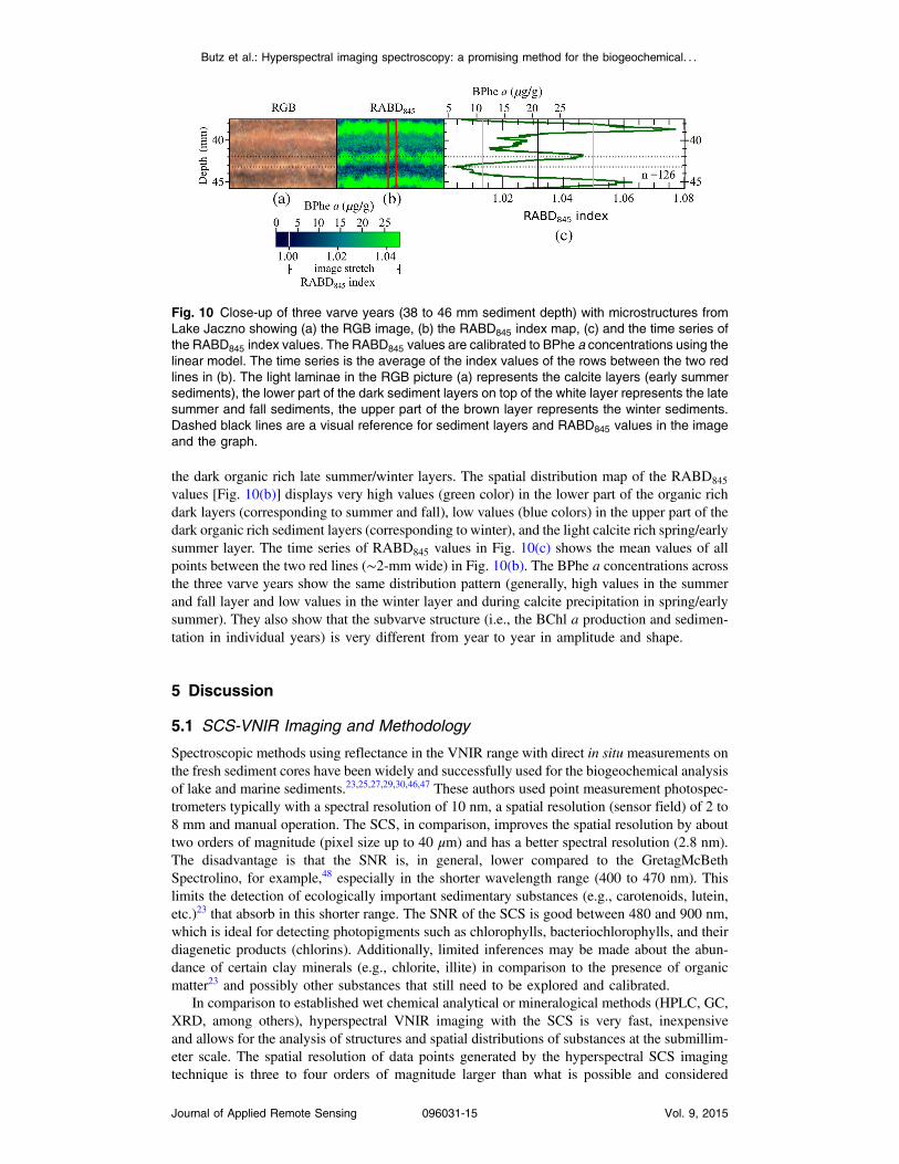
the dark organic rich late summer/winter layers. The spatial distribution map of the RABD845

values [Fig. 10(b)] displays very high values (green color) in the lower part of the organic richdark layers (corresponding to summer and fall), low values (blue colors) in the upper part of thedark organic rich sediment layers (corresponding to winter), and the light calcite rich spring/earlysummer layer. The time series of RABD845 values in Fig. 10(c) shows the mean values of allpoints between the two red lines (∼2-mm wide) in Fig. 10(b). The BPhe a concentrations acrossthe three varve years show the same distribution pattern (generally, high values in the summerand fall layer and low values in the winter layer and during calcite precipitation in spring/earlysummer). They also show that the subvarve structure (i.e., the BChl a production and sedimen-tation in individual years) is very different from year to year in amplitude and shape.

5 Discussion

5.1 SCS-VNIR Imaging and Methodology

Spectroscopic methods using reflectance in the VNIR range with direct in situ measurements onthe fresh sediment cores have been widely and successfully used for the biogeochemical analysisof lake and marine sediments.23,25,27,29,30,46,47 These authors used point measurement photospec-trometers typically with a spectral resolution of 10 nm, a spatial resolution (sensor field) of 2 to8 mm and manual operation. The SCS, in comparison, improves the spatial resolution by abouttwo orders of magnitude (pixel size up to 40 μm) and has a better spectral resolution (2.8 nm).The disadvantage is that the SNR is, in general, lower compared to the GretagMcBethSpectrolino, for example,48 especially in the shorter wavelength range (400 to 470 nm). Thislimits the detection of ecologically important sedimentary substances (e.g., carotenoids, lutein,etc.)23 that absorb in this shorter range. The SNR of the SCS is good between 480 and 900 nm,which is ideal for detecting photopigments such as chlorophylls, bacteriochlorophylls, and theirdiagenetic products (chlorins). Additionally, limited inferences may be made about the abun-dance of certain clay minerals (e.g., chlorite, illite) in comparison to the presence of organicmatter23 and possibly other substances that still need to be explored and calibrated.

In comparison to established wet chemical analytical or mineralogical methods (HPLC, GC,XRD, among others), hyperspectral VNIR imaging with the SCS is very fast, inexpensiveand allows for the analysis of structures and spatial distributions of substances at the submillim-eter scale. The spatial resolution of data points generated by the hyperspectral SCS imagingtechnique is three to four orders of magnitude larger than what is possible and considered

Fig. 10 Close-up of three varve years (38 to 46 mm sediment depth) with microstructures fromLake Jaczno showing (a) the RGB image, (b) the RABD845 index map, (c) and the time series ofthe RABD845 index values. The RABD845 values are calibrated to BPhe a concentrations using thelinear model. The time series is the average of the index values of the rows between the two redlines in (b). The light laminae in the RGB picture (a) represents the calcite layers (early summersediments), the lower part of the dark sediment layers on top of the white layer represents the latesummer and fall sediments, the upper part of the brown layer represents the winter sediments.Dashed black lines are a visual reference for sediment layers and RABD845 values in the imageand the graph.



“high resolution” with wet chemical techniques (e.g., for photopigment analysis by HPLC).30,40

The methodology outlined in Sec. 2 of this article is customized for scientists not familiar withremote sensing technologies, enabling them to acquire high-quality data and generate standardoutput products for spectral indices and sediment proxies that are well established in the envi-ronmental and paleoclimate literature (Refs. 23, 25, 30, and references therein).

5.2 Species Identification and Calibration of Spectral Indices

One of the major challenges that remains is the attribution of spectral properties (i.e., indices,endmembers) of lake sediments to specific substances present in the sediment matrix. Lake sedi-ments can contain a large number of organic and inorganic substances,13 all of which influencethe spectral reflectance (i.e., mixing of spectral signals). This means that diagnostic absorptionbands only occur in rare cases and only for a few dominant substances (e.g., chlorophylls, bac-teriochlorophylls, etc.). Thus, calibration of spectral properties with established quantitative andspecific chemical and physical methods is essential. One problem is that VNIR spectroscopytakes a two-dimensional picture of the sediment surface, while chemical analyses are performedon a three-dimensional volumetric sample. This is particularly the case in sediments withvery high spatial variability, such as varved sediments, as demonstrated in our case study.Consequently, accurate sampling of the sediments used for calibration is particularly important.Sections that are as homogenous as possible and have sufficient sample mass to perform thechemical analyses are ideal.

The calculation of the spectral indices is another important factor and the method should becarefully chosen. Pigment concentrations can be either derived from RABD or from relativeabsorption band areas (RABA).23,32 Either way, the selection of the bands may influence theresult to a certain degree. In this study, we have chosen to use unfiltered reflectance datawith a proven RABD algorithm as a basic approach. The bands used for calculations havebeen carefully selected using endmember analysis and continuum removal. However, furtherpreprocessing of the input data (e.g., spectral smoothing) or the use of a RABA approachmay enhance the calibration.

The performance of the linear calibration model for RABD845 values and BPhe a concen-trations [Fig. 9(a)] is comparable to previous studies where different substances (i.e., chl a,chlorin, lutein, Corg and mineral group ratios) were calibrated to reflectance spectroscopydata from lake and marine sediments.21,2332,49 Comparison of the regression models showedthat the linear model (valid for BPhe a concentrations <28 μg∕g) performed slightly betterthan the exponential model (valid for BPhe a concentrations <46 μg∕g; Fig. 9).

We used spectral data that were measured directly on the fresh sediments. At least in the casestudy presented here, the calibration statistics did not improve if spectral data from homogenizedwet or dry samples (step 3 of the calibration methodology; Sec. 3.1) were used instead of thespectral data from the sediment core image. Although this needs further testing with other lakesediments, it suggests that in situ spectral measurements made directly on fresh sediments aresuitable for calibration purposes.

5.3 Sedimentary BPhe a Distribution in Lake Sediments (Our Case Study)

The calibration of RABD845 to BPhe a (HPLC) revealed that concentrations of BPhe a in theLake Jaczno sediment core could be estimated from hyperspectral data with an uncertainty ofjust 10%. Figures 8 and 10 provide a detailed insight into the BPhe a distribution along the entiresediment core (m-scale) and also within individual varves (submillimeter scale). Since one varverepresents 1 year of sedimentation within the lake, a pixel resolution of 70 μm allows analysis ofseasonal patterns. The distribution of BPhe a concentrations within one varve (Fig. 10) is con-sistent with the ecological conditions in the lake during the annual cycle. BPhe a is the diageneticproduct of Bchl a, which is primarily produced by APB. APBs mainly develop in stratifiedlakes with seasonal sequences of hypolimnetic anoxia, which requires high primary productionin the epilimnion (meso- to eutrophic lakes) and strong seasonal or semipermanent temper-ature and chemical stratification (di- or meromictic conditions with a strong thermo- and chemo-cline).42,50,51 Typically, lakes in northeast Poland mix twice a year in spring and fall when the



chemocline is gone and oxic conditions prevail in the entire water body.52 As a consequence,BPhe a production, its sedimentation and concentration in the sediments are low in the springlayer and early summer layer. The early summer layer is clearly defined in the varves by largeamounts of calcite, which contribute to the low BPhe a concentration in the early summer sedi-ments due to very fast precipitation (matrix effect). The situation is reversed in late summer whenthe lake is stratified, anoxia in the hypolimnion is well developed, production and sedimentationof BPhe a are very high and thus, values in the organic-rich dark sediment layer above the lightcalcite layer are very high. In winter, photosynthesis is generally low under ice cover and BPhe aconcentrations in the winter layer (upper part of the organic-rich dark sediments) are low, despitethe establishment of hypolimnetic anoxia.

Generally, the analysis of the three consecutive varves in Fig. 10 also shows that hyperspec-tral SCS data are able to depict differences in the structure and amplitude of BPhe a concen-trations from year to year. Short-term variability of stratification is often controlled bymeteorological phenomena (mainly temperature and wind). However, the full potential of hyper-spectral SCS data to interpret these subvarve structures in terms of climate reconstructions isyet to be investigated.

6 Conclusions and Outlook

This study has introduced a sediment core scanner equipped with hyperspectral VNIR imagingspectroscopy as a promising nondestructive method to study specific biochemical components oflake sediments. The imaging technique is inexpensive and fast compared to established methods,but the hyperspectral information and data need to be calibrated and verified.

The methodology proposed for sample preparation, data acquisition and processing, and gen-eration of a standard set of output (Sec. 2.1) is widely applicable in the study of marine and lakesediments. All procedures are standardized using ENVI/IDL programming interfaces and outputdata can be further processed using R or other software. This standard procedure is designed andcustomized to enable nonspecialists in remote sensing to use this technology and data.

The SNR ratio is best between 470 and 900 nm. This is not ideal for the detection of sedi-mentary carotenoids, which absorb at shorter wavelengths (400 to 450 nm, e.g., lutein) but isvery suitable for the detection of chloropigments and possibly other substances that are yet to beexplored.

Calibration of hyperspectral data to data obtained from specific quantitative chemical orphysical methods remains a challenge. Most critical is the design of the calibration experiment,the selection of the sediment sampling sites, and the analytical work. The proposed methodologyfor the calibration was shown to be successful in our case study, and the calibration statistics ofdirect spectral measurements on the fresh sediment surface (R2 ¼ 0.89, RMSEP ¼ 10%) arecomparable to previous studies. While it requires further testing, this methodology may bewidely applicable to other studies.

Our case study shows that hyperspectral imaging of lake sediments may provide informationabout important environmental variables at high spatial and temporal resolution back in time(70 × 70 μm2∕pixel). In this study, this means tens of data points within 1 year of sedimentdeposition, which is about three orders of magnitude better than what is possible with wet chemi-cal methods.

We identify three potential future research areas: (1) hardware development, in particular, theextension of the spectral range to include shorter wavelengths at a higher SNR (380 to 470 nm);(2) further testing with case studies from other types of sediments and matrices, and calibratingmore substances; and (3) exploring the potential of high-resolution hyperspectral data fromvarved lake sediments to reveal information about subseasonal phenomena. Climate reconstruc-tions for the past hundreds to thousands of years based on time series of subseasonally resolvedsediment archives would open new perspectives in climate research.

Acknowledgments

This research has been funded through grants from the Oeschger Centre and the Swiss contri-bution to the enlarged European Union CLIMPOL (PSRP-086/2010). Additional funding hasbeen provided by the Swiss National Science Foundation (200020-134945/1). We would like to



thank the following people for their help and contribution to this research project: Drs. BenjaminAmann, Pascal Küpfer, Krystyna Saunders, and Tobias Schneider.

References

1. A. F. H. Goetz, “Three decades of hyperspectral remote sensing of the Earth: a personalview,” Remote Sens. Environ. 113(Suppl. 1), S5–S16 (2009).

2. L. Polerecky et al., “Modular spectral imaging system for discrimination of pigments incells and microbial communities,” Appl. Environ. Microbiol. 75(3), 758–771 (2009).

3. A. Chennu et al., “Hyperspectral imaging of the microscale distribution and dynamics ofmicrophytobenthos in intertidal sediments,” Limnol. Oceanogr. Methods 11(10), 511–528(2013).

4. F. Van Der Meer and W. Bakker, “Validated surface mineralogy from high-spectral reso-lution remote sensing: a review and a novel approach applied to gold exploration usingAVIRIS data,” Terra Nova 10(2), 112–119 (1998).

5. F. A. Kruse, “Identification and mapping of minerals in drill core using hyperspectralimage analysis of infrared reflectance spectra,” Int. J. Remote Sens. 17(9), 1623–1632(1996).

6. C. Gomez et al., “Soil organic carbon prediction by hyperspectral remote sensing and fieldvis-NIR spectroscopy: an Australian case study,” Geoderma 146(3), 403–411 (2008).

7. M. Haest et al., “Unmixing the effects of vegetation in airborne hyperspectral mineral mapsover the Rocklea Dome iron-rich palaeochannel system (Western Australia),” Remote Sens.Environ. 129, 17–31 (2013).

8. S. Thiemann and H. Kaufmann, “Determination of chlorophyll content and trophic state oflakes using field spectrometer and IRS-1C satellite data in the Mecklenburg Lake District,Germany,” Remote Sens. Environ. 73(2), 227–235 (2000).

9. L. Barillé et al., “Comparative analysis of field and laboratory spectral reflectances ofbenthic diatoms with a modified Gaussian model approach,” J. Exp. Mar. Biol. Ecol.343(2), 197–209 (2007).

10. B. Van Gorp et al., “Ultra-compact imaging spectrometer (UCIS) for in-situ planetarymineralogy: laboratory and field calibration,” Proc. SPIE 8515, 85150G (2012).

11. H. Buddenbaum and M. Steffens, “Mapping the distribution of chemical properties in soilprofiles using laboratory imaging spectroscopy, SVM and PLS regression,” EARSeL eProc.11(1), 25–32 (2012).

12. M. Mortimer et al., “Potential of hyperspectral imaging microscopy for semi-quantitativeanalysis of nanoparticle uptake by protozoa,” Environ. Sci. Technol. 48(15), 8760–8767(2014).

13. W. M. Last and J. Smol, Tracking Environmental Change Using Lake Sediments, Vol. 1,Basin Analysis, Coring, and Chronological Techniques, Kluwer Academic Publishers,Dordrecht, Netherlands (2001).

14. P. Francus et al., “An introduction to image analysis, sediments and paleoenvironments,” inImage Analysis, Sediments and Paleoenvironments, P. Francus, Ed., pp. 1–7, Springer,Netherlands (2004).

15. R. R. Schneider et al., “Color-reflectance measurements obtained from Leg 155 cores,” inProc. ODP Init. Rep., Vol. 155, pp. 97–700, Integrated Ocean Drilling Program (IODP),College Station, TX (1995).

16. J. D. Ortiz et al., “Data report: spectral reflectance observations from recovered sediments,”in Proc. ODP Sci. Results, Vol. 162, 259–264, Integrated Ocean Drilling Program (IODP),College Station, TX (1999).

17. W. L. Balsam et al., “Evaluating optical lightness as a proxy for carbonate content in marinesediment cores,” Mar. Geol. 161(2), 141–153 (1999).

18. W. L. Balsam and B. C. Deaton, “Sediment dispersal in the Atlantic Ocean: evaluation byvisible light spectra,” Rev. Aquat. Sci. 4(4), 411–447 (1991).

19. A. C. Mix et al., “Color reflectance spectroscopy: a tool for rapid characterization of deep-sea sediments,” Proc. ODP Init. Rep, Vol. 138, 67–77, Integrated Ocean Drilling Program(IODP), College Station, TX (1992).



http://dx.doi.org/10.1016/j.rse.2007.12.014

http://dx.doi.org/10.1128/AEM.00819-08

http://dx.doi.org/10.4319/lom.2013.11.511

http://dx.doi.org/10.1046/j.1365-3121.1998.00167.x

http://dx.doi.org/10.1080/01431169608948728

http://dx.doi.org/10.1016/j.geoderma.2008.06.011

http://dx.doi.org/10.1016/S0034-4257(00)00097-3

http://dx.doi.org/10.1016/j.jembe.2006.11.013

http://dx.doi.org/10.1117/12.939475

http://dx.doi.org/10.1021/es500898j

http://dx.doi.org/10.1016/S0025-3227(99)00037-7

20. A. C. Mix et al., “Estimating lithology from nonintrusive reflectance spectra: Leg 138,” inProc. ODP Sci. Results, Vol. 138, 413–427, Proceedings of the Ocean Drilling Program(IODP), College Station, TX (1995).

21. W. L. Balsam and B. C. Deaton, “Determining the composition of late quaternary marinesediments from NUV, VIS, and NIR diffuse reflectance spectra,” Mar. Geol. 134(1), 31–55(1996).

22. S. E. Harris and A. C. Mix, “Pleistocene precipitation balance in the Amazon Basinrecorded in deep sea sediments,” Quat. Res. 51(1), 14–26 (1999).

23. B. Rein and F. Sirocko, “In-situ reflectance spectroscopy-analysing techniques forhigh-resolution pigment logging in sediment cores,” Int. J. Earth Sci. 91(5), 950–954(2002).

24. B. Rein et al., “El Niño variability off Peru during the last 20, 000 years,” Paleoceanog-raphy 20(4), PA4003 (2005).

25. B. Das et al., “Inferring sedimentary chlorophyll concentrations with reflectance spectros-copy: a novel approach to reconstructing historical changes in the trophic status of mountainlakes,” Can. J. Fish. Aquat. Sci. 62(5), 1067–1078 (2005).

26. K. Saunders et al., “Late Holocene changes in precipitation in northwest Tasmania and theirpotential links to shifts in the Southern Hemisphere westerly winds,” Global PlanetaryChange 92, 82–91 (2012).

27. L. von Gunten et al., “A quantitative high-resolution summer temperature reconstructionbased on sedimentary pigments from Laguna Aculeo, central Chile, back to AD 850,”Holocene 19(6), 873–881 (2009).

28. L. von Gunten et al., “Calibrating biogeochemical and physical climate proxies from non-varved lake sediments with meteorological data: methods and case studies,” J. Paleolimnol.47(4), 583–600 (2012).

29. M. Trachsel et al., “Scanning reflectance spectroscopy (380-730 nm): a novel method forquantitative high-resolution climate reconstructions from minerogenic lake sediments,”J. Paleolimnol. 44(4), 979–994 (2010).

30. B. Amann et al., “Spring temperature variability and eutrophication history inferred fromsedimentary pigments in the varved sediments of Lake Żabińskie, north-eastern Poland, AD1907–2008,” Global Planetary Change 123, 86–96 (2014).

31. R. D. Jong et al., “Late Holocene summer temperatures in the central Andes reconstructedfrom the sediments of high-elevation Laguna Chepical, Chile (32°S),” Clim. Past 9(4),1921–1932 (2013).

32. A. P. Wolfe et al., “Experimental calibration of lake-sediment spectral reflectance to chloro-phyll a concentrations: methodology and paleolimnological validation,” J. Paleolimnol.36(1), 91–100 (2006).

33. H. Karppinen, PFD-xx-V10E data sheet, SPECIM, Spectral Imaging Ltd., http://www.specim.fi/files/pdf/core/datasheets/PFD_Spectral_Camera-v1-14.pdf, (22 June 2015).

34. M. Marmion, “Sensor response and camera functions,” SPECIM, Spectral Imaging Ltd.,Bern, personal communication (2014).

35. P. Mather and M. Koch, Computer Processing of Remotely-Sensed Images: AnIntroduction, John Wiley and Sons, Chichester (2010).

36. R. N. Clark et al., USGS Digital Spectral Library SPLIB06A, US Geological Survey, RestonVirginia (2007).

37. J. Price, “Examples of high resolution visible to near-infrared reflectance spectra and astandardized collection for remote sensing studies,” Int. J. Remote Sens. 16(6), 993–1000(1995).

38. R. N. Clark and T. L. Roush, “Reflectance spectroscopy: Quantitative analysis techniquesfor remote sensing applications,” J. Geophys. Res. 89(B7), 6329–6340 (1984).

39. W. Tylmann et al., “Laminated lake sediments in northeast Poland: distribution, precondi-tions for formation and potential for paleoenvironmental investigation,” J. Paleolimnol.50(4), 487–503 (2013).

40. N. Reuss et al., “Preservation conditions and the use of sediment pigments as a tool forrecent ecological reconstruction in four Northern European estuaries,” Mar. Chem. 95(3),283–302 (2005).



http://dx.doi.org/10.1016/0025-3227(96)00037-0

http://dx.doi.org/10.1006/qres.1998.2008

http://dx.doi.org/10.1007/s00531-002-0264-0

http://dx.doi.org/10.1029/2004PA001099

http://dx.doi.org/10.1029/2004PA001099

http://dx.doi.org/10.1139/f05-016

http://dx.doi.org/10.1177/0959683609336573

http://dx.doi.org/10.1007/s10933-012-9582-9

http://dx.doi.org/10.1007/s10933-010-9468-7

http://dx.doi.org/10.5194/cp-9-1921-2013

http://dx.doi.org/10.1007/s10933-006-0006-6

http://www.specim.fi/files/pdf/core/datasheets/PFD_Spectral_Camera-v1-14.pdf




http://dx.doi.org/10.1080/01431169508954459

http://dx.doi.org/10.1029/JB089iB07p06329

http://dx.doi.org/10.1007/s10933-013-9741-7

http://dx.doi.org/10.1016/j.marchem.2004.10.002

41. H. Scheer, “An overview of chlorophylls and bacteriochlorophylls: biochemistry, bio-physics, functions and applications,” in Chlorophylls and Bacteriochlorophylls, pp. 1–26,Springer (2006).

42. J. Ji et al., “Centennial blooming of anoxygenic phototrophic bacteria in Qinghai Lakelinked to solar and monsoon activities during the last 18, 000 years,” Quat. Sci. Rev. 28(13),1304–1308 (2009).

43. M. J. Coolen and J. Overmann, “Analysis of subfossil molecular remains of purple sulfurbacteria in a lake sediment,” Appl. Environ. Microbiol. 64(11), 4513–4521 (1998).

44. J. Fiedor et al., “Photodynamics of the bacteriochlorophyll-carotenoid system. 2. Influenceof central metal, solvent and β‐carotene on photobleaching of bacteriochlorophyll deriva-tives,” Photochem. Photobiol. 76(2), 145–152 (2002).

45. R. L. Airs et al., “Development and application of a high resolution liquid chromatographicmethod for the analysis of complex pigment distributions,” J. Chromatogr. A 917(1), 167–177 (2001).

46. N. Michelutti et al., “Recent primary production increases in arctic lakes,” Geophys. Res.Lett. 32(19), L19715 (2005).

47. N. Michelutti et al., “Do spectrally inferred determinations of chlorophyll a reflect trends inlake trophic status?,” J. Paleolimnol. 43(2), 205–217 (2010).

48. B. Rein, In-situ Reflektionsspektroskopie und digitale Bildanalyse: Gewinnunghochauflösender Paläoumweltdaten mit fernerkundlichen Methoden, Habilitation Thesis,p. 104, University of Mainz, Mainz (2003).

49. B. Amann et al., “A millennial-long record of warm season precipitation and flood fre-quency for the North-western Alps inferred from varved lake sediments: implications forthe future,” Quat. Sci. Rev. 115, 89–100 (2015).

50. M. T. Madigan and D. O. Jung, “An overview of purple bacteria: systematics, physiology,and habitats,” in The Purple Phototrophic Bacteria, pp. 1–15, Springer (2009).

51. H. Van Gemerden and J. Mas, “Ecology of phototrophic sulfur bacteria,” in AnoxygenicPhotosynthetic Bacteria, R. Blankenship, M. Madigan, and C. Bauer, Eds., pp. 49–85,Springer, Netherlands (1995).

52. A. Bonk et al., “Modern limnology, sediment accumulation and varve formation processesin Lake Żabińskie, northeastern Poland: comprehensive process studies as a key to under-stand the sediment record,” J. Limnol. 73(AoP), 358–370 (2014).

Biographies for the authors are not available.



http://dx.doi.org/10.1016/j.quascirev.2008.12.015

http://dx.doi.org/10.1562/0031-8655(2002)076%3C0145:POTBCS%3E2.0.CO;2

http://dx.doi.org/10.1016/S0021-9673(01)00663-X

http://dx.doi.org/10.1029/2005GL023693

http://dx.doi.org/10.1029/2005GL023693

http://dx.doi.org/10.1007/s10933-009-9325-8

http://dx.doi.org/10.1016/j.quascirev.2015.03.002

http://dx.doi.org/10.4081/jlimnol.2014.1117

hyperspectral imaging spectroscopy: a promising method for ... · butz et al.: hyperspectral...

Documents