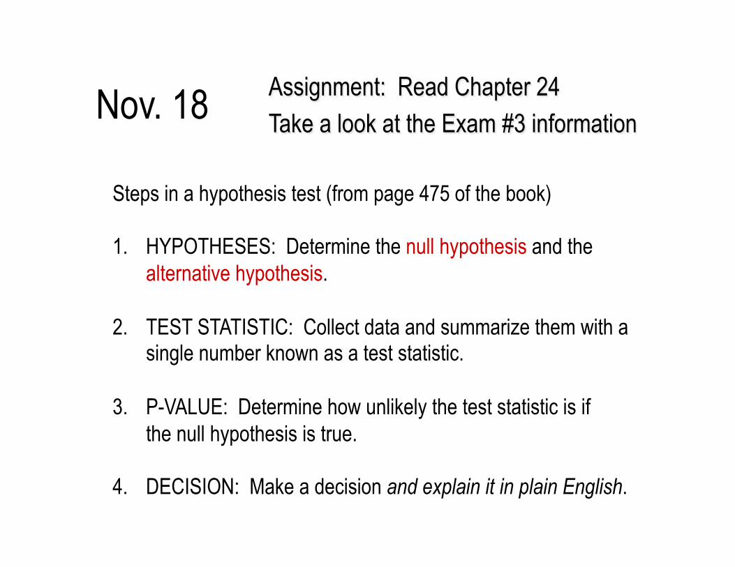
Steps in a hypothesis test (from page 475 of the book) 1.  HYPOTHESES: Determine the null hypothesis and the

alternative hypothesis. 2.  TEST STATISTIC: Collect data and summarize them with a

single number known as a test statistic. 3.  P-VALUE: Determine how unlikely the test statistic is if

the null hypothesis is true. 4.  DECISION: Make a decision and explain it in plain English.

Nov. 18 Assignment: Read Chapter 24 Take a look at the Exam #3 information

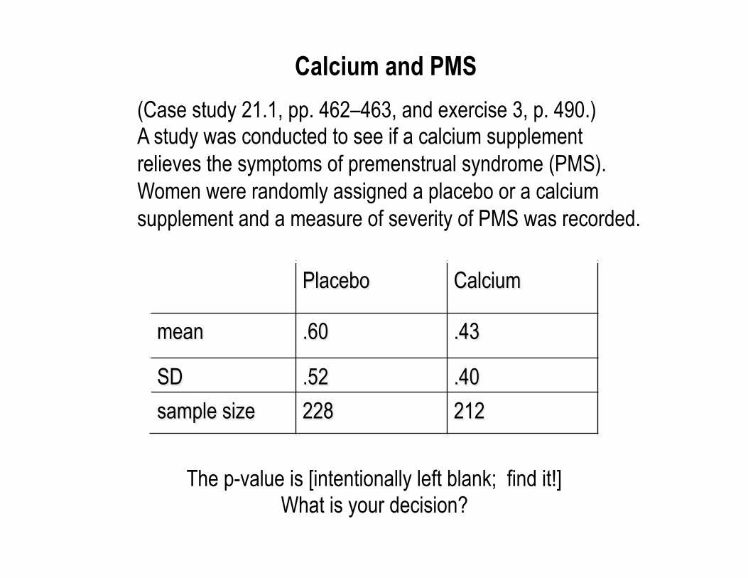
(Case study 21.1, pp. 462–463, and exercise 3, p. 490.) A study was conducted to see if a calcium supplement relieves the symptoms of premenstrual syndrome (PMS). Women were randomly assigned a placebo or a calcium supplement and a measure of severity of PMS was recorded.

Placebo Calcium

mean .60 .43

SD .52 .40 sample size 228 212

The p-value is [intentionally left blank; find it!] What is your decision?

Calcium and PMS

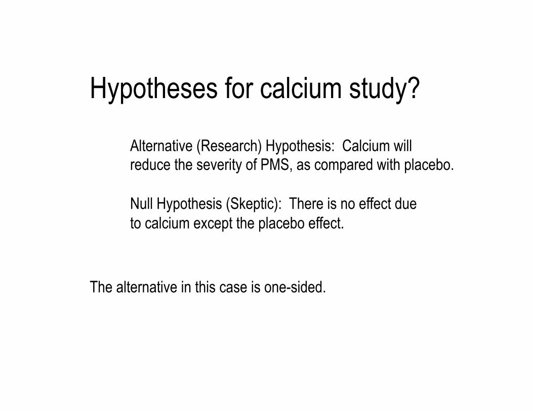
Hypotheses for calcium study?

Alternative (Research) Hypothesis: Calcium will reduce the severity of PMS, as compared with placebo. Null Hypothesis (Skeptic): There is no effect due to calcium except the placebo effect.

The alternative in this case is one-sided.

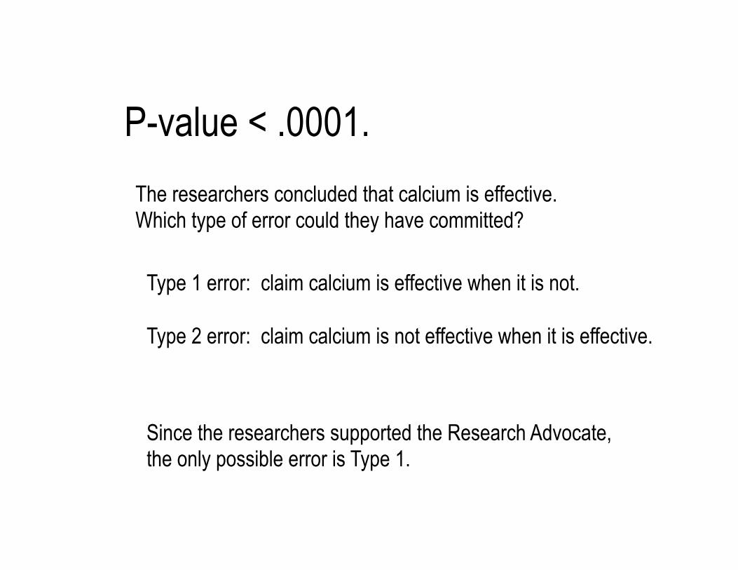
The researchers concluded that calcium is effective. Which type of error could they have committed?

Type 1 error: claim calcium is effective when it is not. Type 2 error: claim calcium is not effective when it is effective.

Since the researchers supported the Research Advocate, the only possible error is Type 1.

P-value < .0001.

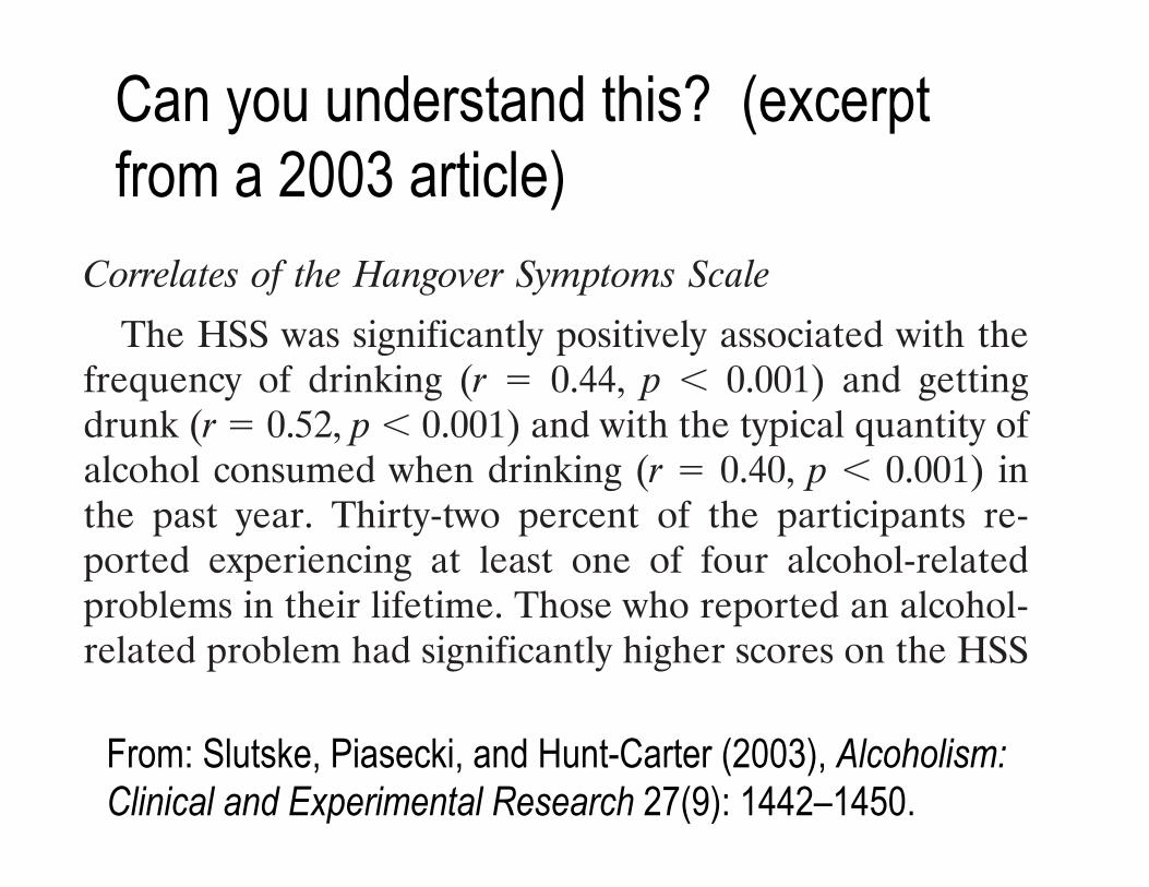
Can you understand this? (excerpt from a 2003 article)

hangover. The single best indicator (across approaches tocombining items) was feeling very weak and the worstindicator was having a lot of trouble sleeping.

The mean score on the hangover scale in which thedichotomous approach to combining items was used was5.2 (SD ! 3.4, range ! 0–13), indicating that, on average,participants reported experiencing about 5 out of 13 differ-ent hangover symptoms during the past year. The meanscore on the hangover scale in which the polytomous ap-proach to combining items was used was 8.3 (SD ! 6.9,range ! 0–49). The dichotomous approach to combiningsymptom items yielded a more normally distributed scale(skewness ! 0.098, SE of skewness ! 0.070, kurtosis !"0.923, SE of kurtosis ! 0.140) than the polytomous ap-proach to combining symptom items (skewness ! 1.217, SEof skewness ! 0.070, kurtosis ! 2.276, SE of kurtosis !0.141). Therefore, in the following section, we present theresults of analyses that used the hangover symptom scalebased on the dichotomous approach to combining symp-toms. The approach used to combine the symptoms did notaffect the results of the correlational analyses below.

There are many research contexts in which it may not befeasible to administer a full 13-item inventory of hangoversymptoms. Thus, we also examined the reliability and va-lidity of a 5-item short-form hangover symptoms scale. The5 items were selected based on the relative magnitude oftheir factor loadings in the principal components analysis(see Table 4) and their item-scale correlations. The fivebest indicators of hangover retained in the 5-item shortform were: more tired than usual, headache, nauseous, feltvery weak, and had difficulty concentrating. The internalconsistency reliability for the 5-item short-form scaleformed using the dichotomous approach to combiningitems was 0.79 and the item-scale correlations ranged from0.53–0.62. The correlates of the 5-item short form of thehangover symptoms scale were nearly identical to those ofthe full 13-item scale.

The psychometric properties of the full and short-formversions of the HSS were similar for men and women. Theinternal consistency reliability of the full version of the HSSwas 0.83 among men and 0.84 among women and the sameset of 5 items selected for the short form of the HSS had thelargest item-scale correlations in both men and women.The internal consistency reliability of the short form of theHSS was 0.78 among men and 0.80 among women.

Correlates of the Hangover Symptoms Scale

The HSS was significantly positively associated with thefrequency of drinking (r ! 0.44, p # 0.001) and gettingdrunk (r ! 0.52, p # 0.001) and with the typical quantity ofalcohol consumed when drinking (r ! 0.40, p # 0.001) inthe past year. Thirty-two percent of the participants re-ported experiencing at least one of four alcohol-relatedproblems in their lifetime. Those who reported an alcohol-related problem had significantly higher scores on the HSS

than those who did not (no alcohol-related problems: mean! 4.3, SD ! 3.3; alcohol-related problems: mean ! 7.0,SD ! 3.0; t ! 13.64, df ! 1225, p # 0.001). Twenty-threepercent of the participants reported that one or both oftheir biological parents had a history of at least one of fouralcohol-related problems (18% fathers only, 3% mothersonly, 2% both parents). Those who reported that one orboth biological parents had a history of an alcohol-relatedproblem had significantly higher scores on the HSS thanthose who did not (no parental alcohol-related problems:mean ! 4.9, SD ! 3.4; parental alcohol-related problems:mean ! 5.9, SD ! 3.6; t ! 4.03, df ! 1225, p # 0.001).Scores on the HSS did not differ for men and women (men:mean ! 5.3, SD ! 3.4; women: mean ! 5.1, SD ! 3.4; t !0.80, df ! 1227, p ! 0.423).

Next, we examined the association of the HSS withalcohol-related problems after controlling for the fre-quency of drinking and getting drunk and the typical quan-tity of alcohol consumed when drinking in the past year.Similar analyses were also conducted examining the asso-ciations of the HSS with parental alcohol-related problemsand with sex. Alcohol-related problems (beta ! 0.196, t !7.70, df ! 1, p # 0.001) and parental alcohol-related prob-lems (beta ! 0.087, t ! 3.61, df ! 1, p # 0.001) remainedsignificant correlates of the HSS, and a significant differ-ence between men and women (with women now havinghigher scores) emerged (beta ! 0.128, t ! 4.89, df ! 1, p #0.001) after controlling for the frequency of drinking andgetting drunk and the typical quantity of alcohol consumedwhen drinking in the past year. Finally, all of the correlatesof the HSS were entered into a single regression model inwhich the frequency of drinking and getting drunk and thetypical quantity of alcohol consumed when drinking in thepast year were controlled. All three of the previously-examined correlates continued to remain significantly as-sociated with the HSS (alcohol-related problems: beta !0.181, t ! 7.11, df ! 1, p # 0.001; parental alcohol-relatedproblems: beta ! 0.066, t ! 2.76, df ! 1, p ! 0.006; femalesex: beta ! 0.120, t ! 4.70, df ! 1, p # 0.001). Theassociations of the HSS with alcohol use, alcohol-relatedproblems, and parental alcohol-related problems did notdiffer for men and women.

DISCUSSION

Alcohol hangover deserves more systematic research at-tention, and standardized, brief hangover assessments areneeded to encourage hangover research. To be maximallyuseful, a hangover measure should assess multiple symp-tom domains, should not rely on respondents’ idiosyncraticdefinitions of hangover, and should be written in such a waythat it taps the “morning after” effects that jibe with classicnotions of the hangover construct. In this research, wesought to develop and evaluate a measure with these prop-erties. The Hangover Symptom Scale (HSS) was con-structed to obtain reports of the frequency with which

DEVELOPMENT OF THE HANGOVER SYMPTOMS SCALE 1447

From: Slutske, Piasecki, and Hunt-Carter (2003), Alcoholism: Clinical and Experimental Research 27(9): 1442–1450.

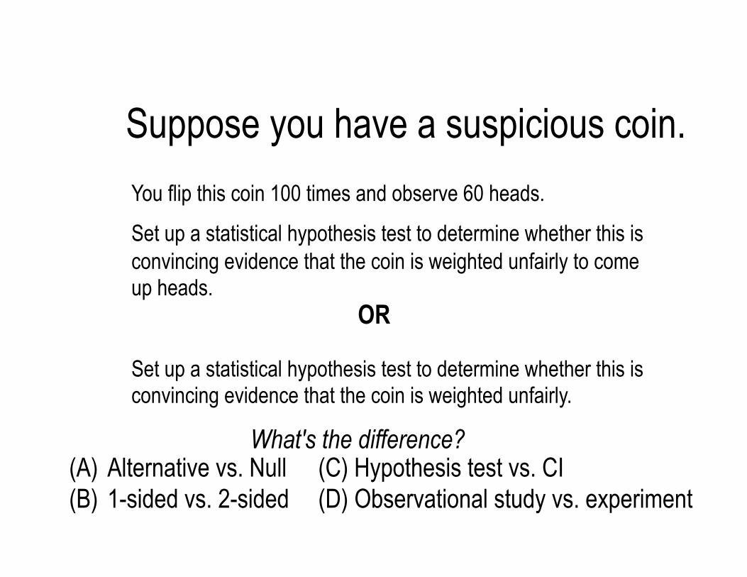
Suppose you have a suspicious coin. You flip this coin 100 times and observe 60 heads.

Set up a statistical hypothesis test to determine whether this is convincing evidence that the coin is weighted unfairly to come up heads.

Set up a statistical hypothesis test to determine whether this is convincing evidence that the coin is weighted unfairly.

OR

What's the difference? (A)  Alternative vs. Null (B)  1-sided vs. 2-sided

(C) Hypothesis test vs. CI (D) Observational study vs. experiment

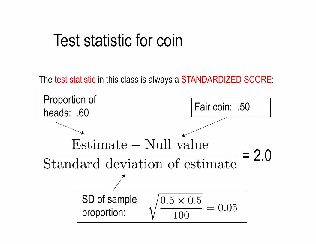
The test statistic in this class is always a STANDARDIZED SCORE:

Test statistic for coin

Proportion of heads: .60 Fair coin: .50

SD of sample proportion:

= 2.0 Estimate�Null value

Standard deviation of estimate

r0.5⇥ 0.5

100= 0.05

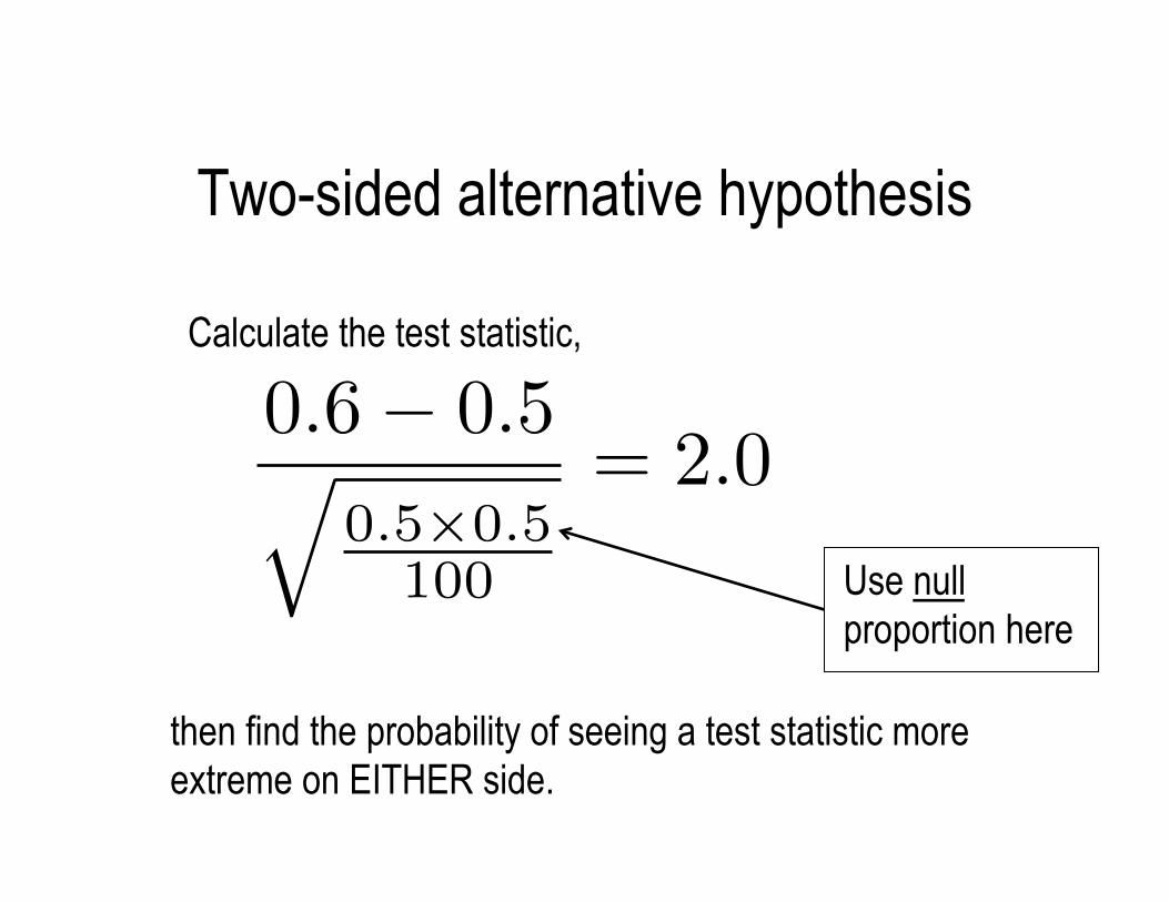
Two-sided alternative hypothesis

Calculate the test statistic,

then find the probability of seeing a test statistic more extreme on EITHER side.

Use null proportion here

0.6� 0.5q0.5⇥0.5

100

= 2.0

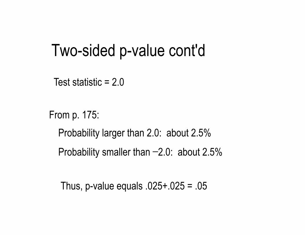
Two-sided p-value cont'd

Test statistic = 2.0

Probability larger than 2.0: about 2.5%

Probability smaller than −2.0: about 2.5%

From p. 175:

Thus, p-value equals .025+.025 = .05

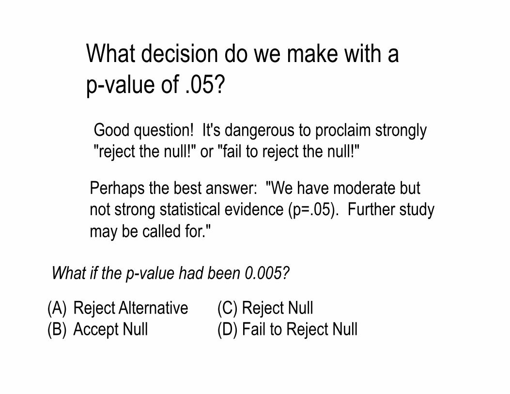
What decision do we make with a p-value of .05? Good question! It's dangerous to proclaim strongly "reject the null!" or "fail to reject the null!"

Perhaps the best answer: "We have moderate but not strong statistical evidence (p=.05). Further study may be called for."

What if the p-value had been 0.005?

(A)  Reject Alternative (B)  Accept Null

(C) Reject Null (D) Fail to Reject Null

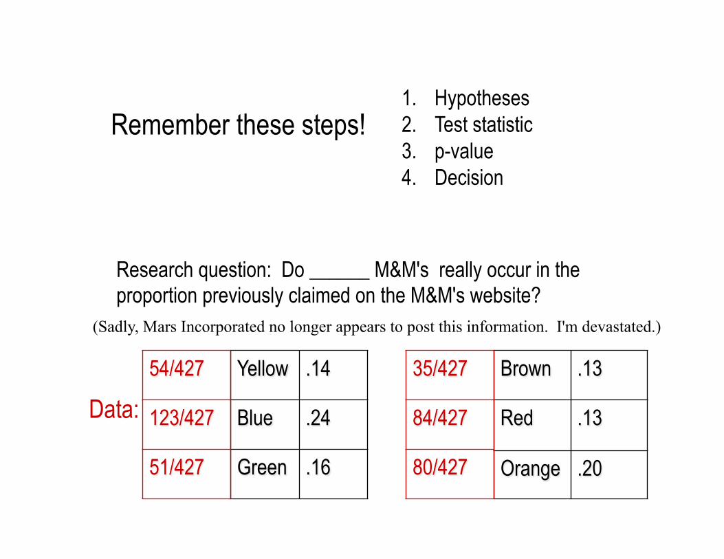
1.  Hypotheses 2.  Test statistic 3.  p-value 4.  Decision

Remember these steps!

Research question: Do ______ M&M's really occur in the proportion previously claimed on the M&M's website?

(Sadly, Mars Incorporated no longer appears to post this information. I'm devastated.)

Yellow .14

Blue .24

Green .16

Brown .13

Red .13

Orange .20

54/427

123/427

51/427

35/427

84/427

80/427

Data:

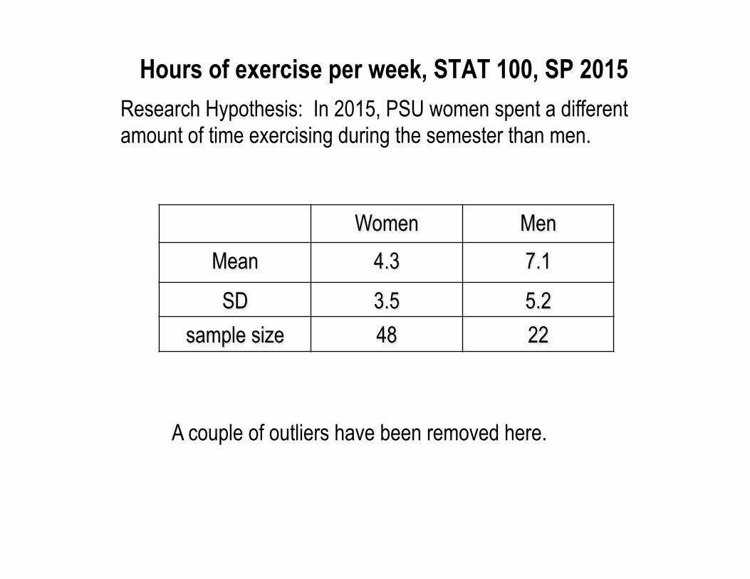
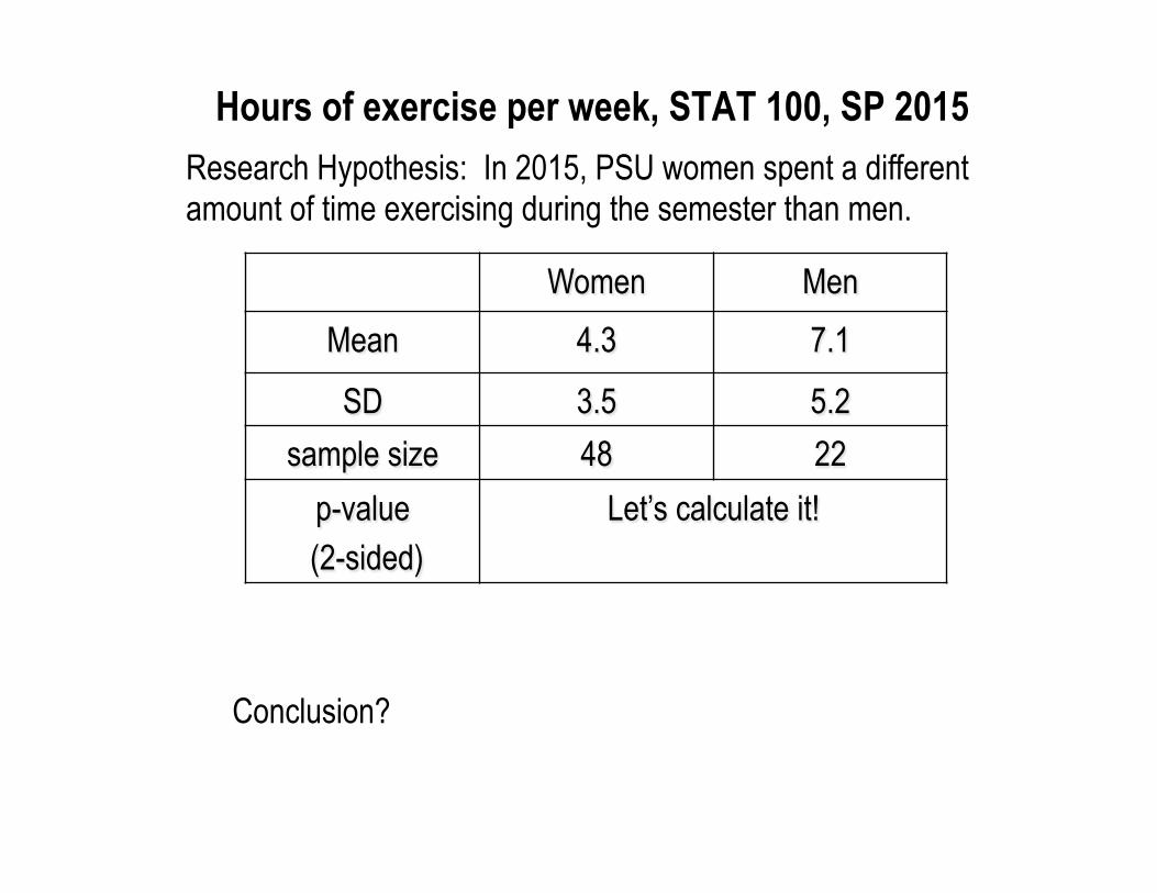
Research Hypothesis: In 2015, PSU women spent a different amount of time exercising during the semester than men.

Hours of exercise per week, STAT 100, SP 2015

Women Men Mean 4.3 7.1

SD 3.5 5.2 sample size 48 22

A couple of outliers have been removed here.

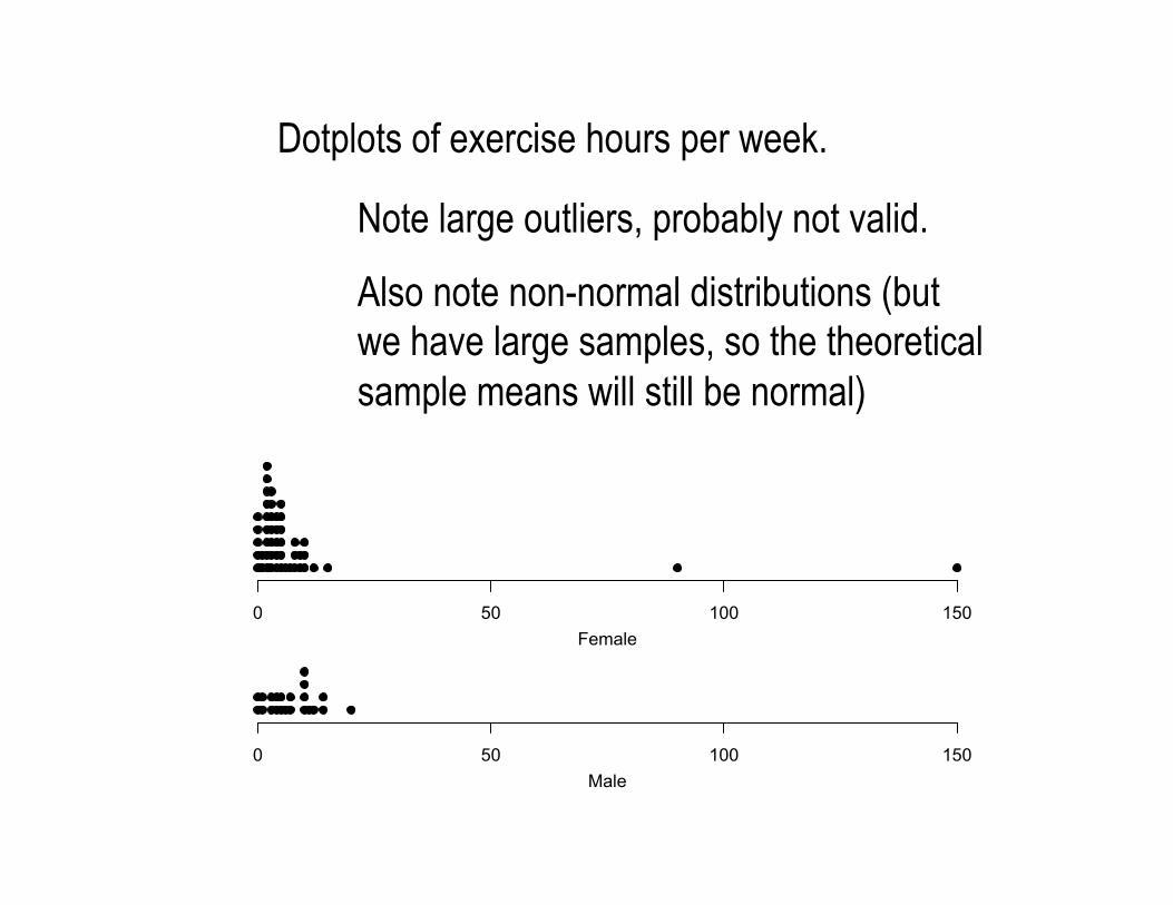
Dotplots of exercise hours per week.

Note large outliers, probably not valid.

Also note non-normal distributions (but we have large samples, so the theoretical sample means will still be normal)

0 50 100 150Female

0 50 100 150Male

Dotplots of exercise hours per week, outliers removed

0 5 10 15 20Female

0 5 10 15 20Male

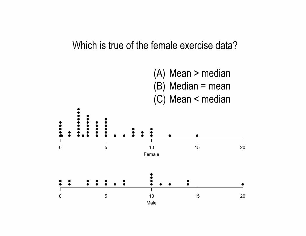
(A)  Mean > median (B)  Median = mean (C) Mean < median

Which is true of the female exercise data?

0 5 10 15 20Female

0 5 10 15 20Male

Research Hypothesis: In 2015, PSU women spent a different amount of time exercising during the semester than men.

Hours of exercise per week, STAT 100, SP 2015

Women Men Mean 4.3 7.1

SD 3.5 5.2 sample size 48 22

p-value (2-sided)

Let’s calculate it!

Conclusion?

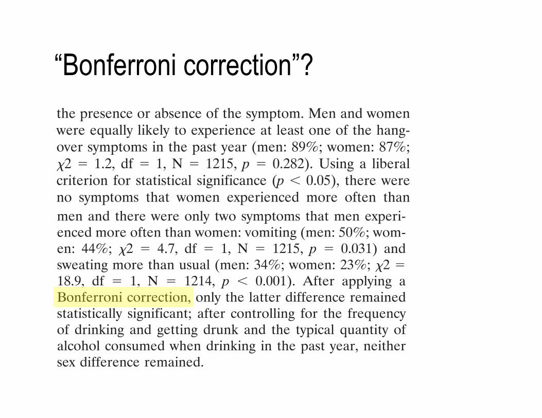
“Bonferroni correction”?

men and there were only two symptoms that men experi-enced more often than women: vomiting (men: 50%; wom-en: 44%; !2 ! 4.7, df ! 1, N ! 1215, p ! 0.031) andsweating more than usual (men: 34%; women: 23%; !2 !18.9, df ! 1, N ! 1214, p " 0.001). After applying aBonferroni correction, only the latter difference remainedstatistically significant; after controlling for the frequencyof drinking and getting drunk and the typical quantity ofalcohol consumed when drinking in the past year, neithersex difference remained.

Men reported drinking more frequently (!2 ! 53.7, df !3, N ! 1211, p " 0.001), getting drunk more frequently(!2 ! 42.9, df ! 4, N ! 1209, p " 0.001), and typicallyconsuming much more alcohol per drinking occasion (!2 !228.5, df ! 4, N ! 1214, p " 0.001) in the past year than didwomen (see Table 2). Controlling for the frequency ofdrinking and getting drunk and for the typical quantity ofalcohol consumed when drinking uncovered a number ofdifferences between men and women not evident in theprevious set of analyses. After controlling for the frequencyof drinking and getting drunk and for the typical quantity ofalcohol consumed when drinking, women were significantlymore likely than men to experience at least one of thehangover symptoms (!2 ! 5.0, df ! 1, N ! 1216, p !0.026), and were also significantly more likely to experience9 of the 13 individual hangover symptoms (thirsty/dehy-drated, more tired than usual, headache, nauseous, weak,difficulty concentrating, more sensitive to light and sound,anxious, and trembling or shaking). Of these, 5 differencesremained significant even after applying a Bonferroni cor-rection (thirsty/dehydrated, more tired than usual, head-ache, nauseous, weak).

Development of the Hangover Symptoms Scale

A principal components analysis of the 13 hangoversymptom items was conducted. There were two principalcomponents with eigenvalues greater than one (eigenvaluesof 5.1 and 1.2) that accounted for 39% and 9% of thevariance in the symptoms, respectively. A one-factor modelwas judged to be preferable to a two-factor model of hang-over symptoms because: a) the items were all significantlyintercorrelated (rs ! 0.18–0.56, all ps " 0.001); b) thefactor loadings were uniformly high in the one-factor model(i.e., the mean factor loading was 0.62 and all of the load-ings were greater than 0.42; see Table 4); c) the compo-nents in the two-factor model were strongly correlated witheach other (r ! 0.61); d) the second component did notaccount for a large portion of variance; and, e) the fiveitems that had modest loadings on the first component andsubstantial loadings on the second component were alsothe five items with the lowest prevalences (sweating, trou-ble sleeping, anxious, depressed, and trembling or shaking;see Table 1) suggesting that these two components werenot identifying meaningful clusters of hangover symptomsbut were instead reflecting psychometric properties of the

items. Experts have convincingly demonstrated in MonteCarlo studies that the popular rule-of-thumb of retainingthe number of factors corresponding to the number ofeigenvalues greater than one is not an effective strategy foridentifying the correct number of factors, and that it oftenleads to retaining too many factors (Cliff, 1988; Fabrigar etal., 1999), therefore we did not rely on the eigenvalues-greater-than-one rule in selecting the proper model. Thefactor loadings from the one-factor model are shown inTable 4. The results of the principal components analysesjustified combining the 13 hangover symptoms into a singlescale.

Table 4 also presents the results of conducting principalcomponents analyses separately for the men and thewomen in the sample. The results of the analyses stratifiedby sex led to the same conclusion as the analysis of the fullsample, and the results for men and women were verysimilar (the factor loadings presented in Table 4 for menand women correlated 0.76).

We examined two different approaches to combining thehangover symptom items. In the first approach (which wewill call the “dichotomous” approach), each 5-level itemwas dichotomized according to whether the symptom neveroccurred or ever occurred, and these 13 dichotomous itemswere summed to form a scale with a possible range of 0–13.This approach to combining items yields a scale that em-phasizes the diversity of hangover symptoms occurringwithin the past year; the internal consistency reliability(coefficient alpha) for the scale formed using this approachwas 0.84 and the item-scale correlations ranged from 0.32–0.62. In the second approach (which we will call the “poly-tomous” approach), the original 5-level items weresummed to form a scale with a possible range of 0–52. Thisapproach to combining items emphasizes the pervasivenessas well as the diversity of hangover symptoms occurringwithin the past year; the internal consistency reliability(coefficient alpha) for the scale formed using this approachwas 0.86 and the item-scale correlations ranged from 0.35–0.68. All of the items appeared to be adequate indicators of

Table 4. Factor Loadings From Principal Components Analyses of Past-YearHangover Symptoms

Symptom

Allparticipants(n ! 1205)

Men(n ! 454)

Women(n ! 725)

Felt extremely thirsty or dehydrated 0.62 0.64 0.61Felt more tired than usual 0.73 0.68 0.75Experienced a headache 0.68 0.65 0.70Felt very nauseous 0.68 0.65 0.71Vomited 0.52 0.46 0.55Felt very weak 0.76 0.73 0.79Had difficulty concentrating 0.72 0.74 0.70More sensitive to light and sound than usual 0.63 0.66 0.60Sweated more than usual 0.62 0.68 0.59Had a lot of trouble sleeping 0.43 0.48 0.42Was anxious 0.55 0.63 0.49Felt depressed 0.53 0.51 0.53Experienced trembling or shaking 0.55 0.59 0.53

Eigenvalue 5.1 5.1 5.0% Variance 39 40 39

1446 SLUTSKE ET AL.

RESULTS

For both sets of hangover symptoms items – those basedon the first few lifetime drinking occasions and those basedon the past year drinking occasions – we examined theprevalence of each of the 13 individual hangover symptoms,conducted a principal components analysis of the hangoversymptom items, assessed the psychometric characteristicsof full and short-form versions of the HSS, and evaluatedthe relations of the HSS with alcohol use, alcohol-relatedproblems, parental alcohol-related problems, and sex. Bothsets of items yielded very similar results. The correlationbetween the hangover scales indexing the two differentdrinking epochs was 0.79, indicating a high degree of sta-bility of hangover symptoms and suggesting that there waslittle unique information captured by our assessments ofhangover at the initiation of the drinking career versus inthe past year. Therefore, for all subsequent analyses, weonly present the results of those based on hangover symp-toms that occurred in the past year.

Prevalence of Hangover Symptoms in the Past Year

Descriptive data concerning alcohol involvement in thissample are presented in Table 2. Most of the participantsreported that they had consumed alcohol on between 101and 1000 occasions over their lifetime. The modal age ofonset of drinking in these mostly college-age young adultswas 15–16 years, indicating that the majority of participantshad been drinking for about 2–3 years.

The past-year prevalences of hangover symptoms, basedon responses to HSS items, are presented in Table 1. Themost common hangover symptom was feeling extremelythirsty or dehydrated (72%) and the least common symp-tom was experiencing trembling or shaking (13%). In re-sponse to the hangover count item, 87% of the participantsreported experiencing at least one hangover symptom inthe past year; Table 3 summarizes the responses to thehangover count item for the total sample and for men andwomen separately.

We tested for potential sex differences in individualhangover symptoms using responses to the HSS items. Forthese analyses, each HSS item was dichotomized to reflectthe presence or absence of the symptom. Men and womenwere equally likely to experience at least one of the hang-over symptoms in the past year (men: 89%; women: 87%;!2 ! 1.2, df ! 1, N ! 1215, p ! 0.282). Using a liberalcriterion for statistical significance (p " 0.05), there wereno symptoms that women experienced more often than

Table 2. Characteristics of Alcohol Involvement Among College Students

Variable

All participants(n ! 1211–1225)

(%)

Men(n ! 465–470)

(%)

Women(n ! 746–755)

(%)

Lifetime drinking occasions1–10 13 8 1611–100 36 28 41101–1000 38 43 36#1000 12 21 7

Age first drank (years)"11 4 5 311–14 30 35 2715–16 45 36 5017–18 21 21 20#18 2 2 1

Past-year frequency of drinking"1 day a month 23 16 281–3 days a month 34 30 371–2 days a week 31 38 27"3 days a week 11 17 8

Past-year frequency of getting drunkNever 16 12 19"1 day a month 37 32 411–3 days a month 30 32 291–2 days a week 15 21 11"3 days a week 2 4 1

Past-year typical quantity drank1 drink 10 7 122–3 drinks 24 13 314–5 drinks 33 25 396–7 drinks 19 26 15#7 drinks 14 30 4

Lifetime alcohol-related problems 32 35 30Parental alcohol-related problems 23 23 23

Table 3. Number of Times Experienced at Least One Hangover Symptom inthe Past Year Among College Students

Response

All participants(n ! 1216)

(%)

Men(n ! 466)

(%)

Women(n ! 749)

(%)

0 times 13 11 141–2 times 27 25 283–11 times 34 33 3512–51 times 21 23 20"52 times 5 7 4

DEVELOPMENT OF THE HANGOVER SYMPTOMS SCALE 1445